


Languages
Pages
Legal


Technical University of Munich
Physics department
Advanced practicum in
Femtoscopy
September 2021
Dimitar Mihaylov
Group of Prof. Fabbietti

Contents
Must read
1 Introduction 2
1.1 Goals and requirements . . . . . . . . . . . . . . . . . . . . . . . . . . . . . . . . . . . . . . . . . . 2
1.2 Report and colloquium . . . . . . . . . . . . . . . . . . . . . . . . . . . . . . . . . . . . . . . . . . . 3
1.3 Remote participation . . . . . . . . . . . . . . . . . . . . . . . . . . . . . . . . . . . . . . . . . . . . 4
1.4 Units . . . . . . . . . . . . . . . . . . . . . . . . . . . . . . . . . . . . . . . . . . . . . . . . . . . . . 5
2 Baryon–baryon interaction 6
2.1 Overview . . . . . . . . . . . . . . . . . . . . . . . . . . . . . . . . . . . . . . . . . . . . . . . . . . . 6
2.2 Experimental techniques . . . . . . . . . . . . . . . . . . . . . . . . . . . . . . . . . . . . . . . . . 10
2.3 Neutron stars and the equation of state . . . . . . . . . . . . . . . . . . . . . . . . . . . . . . . . . 10
3 Femtoscopy 13
3.1 Emission source . . . . . . . . . . . . . . . . . . . . . . . . . . . . . . . . . . . . . . . . . . . . . . . 14
3.2 Wave function . . . . . . . . . . . . . . . . . . . . . . . . . . . . . . . . . . . . . . . . . . . . . . . . 15
3.3 Correlation function . . . . . . . . . . . . . . . . . . . . . . . . . . . . . . . . . . . . . . . . . . . . 16
3.4 Experimental data . . . . . . . . . . . . . . . . . . . . . . . . . . . . . . . . . . . . . . . . . . . . . 18
Handbook (during the practicum)
4 Analysis procedure 19
4.1 Tasks . . . . . . . . . . . . . . . . . . . . . . . . . . . . . . . . . . . . . . . . . . . . . . . . . . . . . 19
4.2 Technical details . . . . . . . . . . . . . . . . . . . . . . . . . . . . . . . . . . . . . . . . . . . . . . 20
4.2.1 Basic command line instructions . . . . . . . . . . . . . . . . . . . . . . . . . . . . . . . . 20
4.2.2 Basics of C++ . . . . . . . . . . . . . . . . . . . . . . . . . . . . . . . . . . . . . . . . . . . . 21
4.2.3 Basics of ROOT . . . . . . . . . . . . . . . . . . . . . . . . . . . . . . . . . . . . . . . . . . . 24
4.2.4 All you need within FemtoFopra . . . . . . . . . . . . . . . . . . . . . . . . . . . . . . . . . 27
4.2.5 Interaction potential inside CATS . . . . . . . . . . . . . . . . . . . . . . . . . . . . . . . . 30
4.3 Uncertainty determination . . . . . . . . . . . . . . . . . . . . . . . . . . . . . . . . . . . . . . . . 31
Appendix
A Details on the source function 32
B ALICE experiment 34
1

Chapter 1: Introduction
1.1 Goals and requirements
Within the standard model of physics there are four fundamental interactions: gravitational, electromagnetic,
strong and weak interaction. In this advanced practicum course the focus is on the strong interaction. In
particular, the participants will study the novel methods to investigate hadron–hadron interactions using
momentum correlation techniques. The goal of the practicum is to analyse the correlations between protons
(p) and Λ hyperons produced in proton-proton (pp) collisions at the Large Hadron Collider (LHC). The
corresponding correlation function, measured by the ALICE collaboration, will be fitted in order to extract
several interaction parameters, such as the pΛ cross section. The results will be compared to the existing
scattering data.
The practicum will be divided into two parts, both performed on the same day.
• Physics
The first part of the practicum will be a detailed discussion, related to the physics topic presented
in chapters 2 and 3. The participants are required to read this part of the manual beforehand. Do
not worry if you fail to understand everything, the goal is to set up a good stage to develop a fruitful
discussion, during which an active participation, ideally filled with questions, is expected. Ultimately,
the first half of the practicum aims at providing the students with a basic understanding on the subjects
of final state interaction and femtoscopy.
N.B. All participants are expected to be involved in the discussion and a failure to read the manual,
even by a single group member, may cause rescheduling of the practicum!
• Analysis
The second part of the practicum is to go through the main analysis steps required to convert a
measured yield of pΛ pairs into a cross section. As the software frameworks involved cannot be taught
in few hours, the participants will be provided with an easy to use C++ template class, which can handle
the analysis steps with minimal user input. Note, that it is not mandatory to have good programming
skills to complete this course. Nevertheless, students with good coding skills will be able, should they
desire, to perform additional tasks.
N.B. The participants do not need to prepare anything in advance for this part, all will be explained by
the tutor on the day of the practicum. Chapter 4 will serve as a handbook, and you do not need to read
it in advance. Nevertheless, if you have zero coding skills, it is recommended to familiarise yourself
with section 4.2.2 and find some appropriate online exercises to perform on your own PC.
2

Manual for FOPRA 102 Advanced practicum in Femtoscopy
1.2 Report and colloquium
As this is an advanced practicum, we find it is more beneficial for the students to detach from the mindset of
writing a typical lab report, in favour of practising the writing of a pure scientific text. Hence, the report has
to be structured like a short scientific paper, written in English, but without an abstract. Below the checklist
on which the evaluation will be based:
• A clear read-flow, where the details are omitted, just mentioned and cited. The goal is to practice your
skills in discriminating between relevant and non-relevant information, as you will need to significantly
shorten the lengthy text within the manual.
While you are likely to use only information from this manual, if a particular statement is referenced
within the manual, please use the corresponding reference in the report.
• Introduction to stage the goal of the analysis, i.e. femtoscopy as a tool to study baryon–baryon
interaction, highlighting applications (see section 2.3). This part should be around 1/2 page (maximum
1 page).
• Brief summary of the analysis steps, starting from the theoretical and experimental definition of the
correlation function (1-2 pages). All the models used are to be references, any important relations
employed have to be included.
• Results, including plots and discussion (up to 2 pages).
• Few lines of summary, which may include an outlook with future possible applications of this method.
The colloquium will focus on the physics aspects of the practicum, corresponding to chapters 2 and 3.
Further, the obtained analysis results are to be discussed within the context of the relevant physics. The
colloquium will be very similar to the discussion part of the practicum, where the obvious difference will
be the role of the tutor, which will change from a teacher to a moderator. In short: if you read the manual,
actively participate in the initial discussion and take notes, the job is as good as done.
3

Manual for FOPRA 102 Advanced practicum in Femtoscopy
1.3 Remote participation
The personal contact is still an important part of teaching and learning, thus both the practicum and
colloquium are to be performed at the university. Unfortunately, for the WS21/22 the 3G rule applies
(Geimpft, Genesen, Getestet), which means you have to be either vaccinated, recovered or tested in order to
perform the practicum in person. A certificate to verify that is required. A fast antigen test is offered for free
on campus (https://schnelltest-studitum.de/).
Naturally, in case of a significant reason prohibiting that, COVID related or otherwise, there are options for
remote participation. In such a case, the discussion and colloquium will be on Zoom, however, depending
on the seriousness of the restrictions, there are two options for the analysis.
• Hybrid: The analysis part is to be performed in person by a single group member, while the rest of the
students are connected over Zoom.
• Fully remote: In the unlikely case of a complete lockdown, a Teamviewer session will be set up to
perform the analysis.
4

Manual for FOPRA 102 Advanced practicum in Femtoscopy
1.4 Units
The standard SI units are not very practical and intuitive in the context of quantum systems. The so-called
“natural units” provide a more simplistic notation, as they treat some of the fundamental physics constant
as unitless numbers, arbitrary set to 1. In particular, the speed of light c and the Planck constant ~ are set
to unity, while the unit of energy is eV. Using this notation, one can remove all factors of c or ~ from the
equations. Further, the units of mass and momentum become identical to energy (eV), while the unit of
length is the inverse (1/eV), all of which corresponds nicely to the physics interpretation of these observables.
Nevertheless, it is accustomed to use femtometers (fm), or in short Fermi, as the unit of length. This is
motivated by the comparable scale to the charge radius of the proton (c.a. 0.85 fm). To convert fm to natural
units, or vice versa, it is useful to remember that ~c = 197.327 MeV·fm. For example:
1 fm = 1 fm
~c= 1 fm
197.327 MeV · fm= 1
197.327MeV−1.
Another common convention is to include the factor c within the units, even if it is equal to 1. The reason is to
make possible to separate energy, momentum and mass just by looking at the units. For example, these three
will have, respectively, units of eV, eV/c and eV/c2. Regarding the time, it has the same units as space (1/eV),
but the typical representation is in fm/c. The reasoning is that in particle physics most of the problems are
ultra relativistic, meaning that particles travel at approximately the speed of light. The unit fm/c corresponds
to the time required light to travel 1 fm (3.3 ·10−24 s), providing an intuitive time scale relative to the spacial
extensions.
5

Chapter 2: Baryon–baryon interaction
2.1 Overview
The fundamental theory to study the strong interaction is quantum chromodynamics (QCD). It deals with
the most fundamental property of the strong interaction, the colour charge, and the related fundamental
particles: quarks and gluons. The quarks are thought as elementary particles of matter, that carry colour
charge (red, blue, green), a fractional electric charge (±1/3 or ±2/3) and a flavour (up, down, charm, strange,
top, bottom). The gluons are electrically neutral exchange particles, which carry the colour charge. This is in
big contrast to the photon, which is the exchange particle related to the electromagnetic force, and leads to
the unique QCD feature of gluon self-coupling. Due to the QCD running coupling constant, which becomes
smaller as a function of the energy, the theory is perturbative at very large energies (&GeV). However, even at a
high-energy experiment such as the LHC, the collision system is mostly described by non-perturbative effects,
as the temperature of the system is ∼ 100 MeV just after few fm/c (∼ 10−24 s) after the initial interaction. At
that point the quarks can only be found inside colour neutral composite states, called hadrons (e.g. protons
and neutrons). Describing the subsequent interaction of the hadrons becomes a nearly impossible task
using the fundamental QCD properties, nevertheless there are effective perturbative theories, such as chiral
effective field theory (χEFT) [1], used to model the strong interaction. The hadrons can be composed out of a
quark (q) and an anti-quark (q) or three quarks or anti-quarks of different colour. The former (qq) are called
mesons and the latter (qqq or q q q) are called baryons. If a baryon is composed only of u and d quarks it is
called a nucleon (N), in particular protons (uud) and neutrons (udd), while u, d and s containing baryons
are referred to as hyperons (Y). The nucleons have a mass of approx. 939 MeV/c2, while the lightest hyperon
is called Λ (ud s). It has a mass of 1116 MeV/c2 and is electrically neutral. On the other hand, the lightest
hadrons are the π mesons (pions), which are composed of combinations of u and d quarks and have a mass of
c.a. 140 MeV/c2. Within χEFT the pions act as effective exchange particles among the heavier hadronic states.
This allows to have an intrinsic ordering scheme of the theory, depending on the complexity of the exchange
vertexes (see Fig. 2.1), with each order increasing the precision of the theory, at the price of introducing
more parameters. Unfortunately, apart for protons and neutrons, there is insufficient experimental data to
exploit the higher orders of the theory, e.g. the pΛ system is modelled up to next-to-leading order (NLO)
calculations [1].
In practical terms, the properties of the interaction is often reduced to the basic notation of scattering theory,
as introduced at entry level quantum mechanics books, e.g. by D. J. Griffiths [3] and J. J. Sakurai [4]. Below only
the most relevant relations, without proof, are provided. One of the most simplistic quantitative description
of the interaction is given by the cross section, which is linked to the probability that the two particles in
question interact. It has the units of area, typically barn (1 b = 100 fm2). A large cross section corresponds to
strongly interacting particles, while a shallow potential will result in small values of the cross section. Fig. 2.2
shows an example of the measured (black points) and theoretical cross section corresponding to the pΛ
system. However, the cross section is often insufficient observable to provide differential information, for
6

Manual for FOPRA 102 Advanced practicum in Femtoscopy
Figure 2.1: Hierarchy of nuclear forces up to N3LO of the chiral expansion. Only some representative diagrams areincluded. The plot is taken from [2]. These are like Feynman diagrams, where the solid lines represent the interactingparticles, while the dashed lines are the exchange particles (pions). The interaction vertices are represented by symbols.The chiral expansion is perturbative, meaning that the higher orders are suppressed.
example it cannot discriminate between an attractive and a repulsive interaction. From quantum mechanical
perspective, the full information of the system is provided by the wave function. In the case of two particles,
the single particle quantum formalism can be used, by introducing the effective mass and momentum of the
system (µ and k∗).
µ= m1m2
m1 +m2(2.1)
is called the reduced mass. The momentum is defined as
k∗ = 1
2
∣∣~p∗1 −~p∗
2
∣∣ , (2.2)
where m1,2 are the masses of the two particles and ~p∗1,2 are their momenta evaluated in the pair rest frame
(~p∗1 = −~p∗
2 ). This implies that k∗ corresponds to the absolute value of the single particle momentum. To
investigate the low momentum region (k∗ < 200 MeV/c) it is sufficient to solve the radial Schrödinger
equationd 2ul (k∗,r∗)
dr∗2 =[
2µVl (r∗)+ l (l +1)
r∗2 −k∗2]
ul (k∗,r∗). (2.3)
This equation is defined for a specific partial wave l and a radial symmetric potential Vl (r∗). The total wave
function of the system is
Ψ(~k∗,~r∗) =∞∑
l=0Rl (k∗,r∗)Yl (θ∗) =
∞∑l=0
i l (2l +1)ul (k∗,r∗)
rPl (cosθ∗)︸ ︷︷ ︸
:=Ψl (k∗,r ∗)
, (2.4)
where l is the angular quantum number and Pl are the Legendre polynomials, while ul (k∗,r∗) = r∗Rl (k∗,r∗)
satisfies the radial Schrödinger equation (Eq. 2.3). The low energy (k∗ → 0) scattering can be modelled only
7

Manual for FOPRA 102 Advanced practicum in Femtoscopy
Figure 2.2: Scattering data for the pΛ→pΛ elastic process.Data from [5–7], plot from [1]. The coloured bands are thepredictions of the leading-order (LO) and next-to-leading-order (NLO) χEFT predictions, green and red respectively.The overall agreement of NLO is better, however at low en-ergies the two models cannot be discriminated from oneanother, due to the poor precision of the data.
Figure 2.3: The spherical Besselfunctions jl (k∗r∗) of the first kind.These represent the free wave so-lution ul (k∗,r∗) of the Schrödingerequation (Eq. 2.3). The even l resultin symmetric function, the odd l inanti-symmetric. For l 6= 0 the func-tions converge towards zero.
by taking the first few partial waves l , as ul 6=0(k∗,r∗) converge towards zero, and the convergence is faster
for higher l . This is visually presented in Fig. 2.3, which shows the solution of the Schrödinger equation for
a free wave, i.e. Vl (r∗) = 0. While a non-zero potential will modify the functions, the generic convergence
properties remain similar. An interesting feature of the free wave function is that it cannot be normalised over
space. The typical convention in quantum mechanics is to use the condition |Ψ(k∗,r∗)| = 1. This property
is satisfied by the infinite sum of the Bessel functions. Moreover, for a short ranged potential Vl (r∗) this
condition remains valid, but only in the asymptotic region corresponding to large k∗r∗ values.
The properties of the interaction can be effectively represented in terms of the so-called scattering parameters,
as well the cross section. Typically the experiments are only sensitive to the asymptotic shape of the wave
function, as the particles are measured centimetres to meters away from their interaction point. As it
will become evident in chapter 3, in theory the correlation techniques can probe the non-asymptotic part,
although the leading order effects are still determined by the asymptotic solution. For that reason the effective
8

Manual for FOPRA 102 Advanced practicum in Femtoscopy
parameterization of the interaction is of importance. Since the strong interaction is short ranged, Vl (r∗)
becomes negligible after few femtometers, hence the solution ul (k∗,r∗) of the Schrödinger equation becomes
identical to the free wave solution. Nevertheless, the two cases will have different boundary conditions at
r∗ = 0, thus the solution ul (k∗,r∗) will be shifted by a phase δl , i.e. ul (k∗,r∗) = jl (k∗r∗+δl ). The phase shift
is related to the properties of the potential Vl (r∗). Since the Schrödinger equation is solved for r∗, the phase
shift will not have an implicit r∗ dependence, nevertheless it will depend on k∗. This dependence can be
expanded using the effective range approximation
k ·cot[δ0(k∗)]k∗→0≈ 1
f0+ 1
2d0k∗2 +O (k∗4). (2.5)
Note, that this particular relation is obtained for l = 0 and typically valid for k∗ smaller than 100-200 MeV/c.
The higher partial waves are not relevant for low-energy scattering, which is the main region of interest in the
present practicum, hence the discussion will assume that the interaction if fully determined by the s-wave
(l = 0). In that case, the relevant information is effectively represented by only two parameters: the scattering
length ( f0) and the effective range (d0), where the strength of the potential is reflected in the absolute value of
f0. There are different conventions regarding the sign1 of f0, in femtoscopy the sign convention dictates that
a positive f0 corresponds to a non-binding attractive interaction, while a negative sign can be either a bound
state (if d0 is small) or correspond to a repulsive potential (if d0 is large). These properties can be understood
from the geometrical representation of the wave function, for those interested a good explanation is provided
in the book of J. J. Sakurai [4] (the chapter on scattering theory).
An even more basic parameterization of the interaction is given by the cross section. In an oversimplified
picture (Fig. 2.4), the differential cross section dσ(Ω) is the probability that a particle scatters off the potential
at a spacial angleΩ. The integrated total cross section is denoted by σ. It has units of area, which in nuclear
physics is expressed in barn (1 b = 10−28 m2 = 100 fm2). It is easy to imagine that the probability to interact is
Figure 2.4: Particles incident in the area dσ scatter into the solid angle dΩ. Plot taken from [3].
directly related to the phase shift of the wave function, and indeed it can be shown [3, 4] that
σ(k∗) = 4π
k∗2
∞∑l=0
(2l +1)sin2 [δl (k∗)
]. (2.6)
Traditionally, the interaction between particles has been studied exclusively by measurements of the cross
section, deferentially or integrated. This is due to the easy experimental set up, where in incoming beam of
particles is shot at a target and the deflection of the particles carries information on the elastic interaction. The
1In most quantum mechanics books there is a minus sign in front of 1/ f0 in Eq. 2.5.
9

Manual for FOPRA 102 Advanced practicum in Femtoscopy
cross section, at a fixed energy, provides very little direct information. For example, it cannot discriminate
between an attractive and a repulsive potential. Thus, any results have to be compared to theoretical
predictions capable of simultaneously modelling multiple observables. The energy (k∗) dependence of the
cross section, especially at low energies, is very important to understand the underlying properties of the
potential.
2.2 Experimental techniques
The baryon–baryon interaction is well known for the nucleons (N), as they are the constituents of the stable
matter and thus experimentally accessible. Through sophisticated analyses, e.g. involving a technique
called partial wave analysis, the NN interaction has been determined for the different partial waves and spin
configurations, including details on the coupling effects between spin and orbital momentum, tensor forces
etc. As such, there is no need, and arguably no possibility, to improve on the existing data with alternative
methods. However, the situation is very different when baryons containing strange quarks (hyperons Y) are
involved, such asΛ (uds), Ξ− (dss),Ω− (sss) and others. For these exotic particles, scattering experiments are
almost impossible to realise due to the inability to create a stable beam of these quickly decaying species.
One can stage the production of these particles in other types of collisions and analyse the secondary re-
scattering, but in this way the overall statistics and the information on the initial state are poor. Practically,
such measurements can only be performed for particles containing a single strange quark, such asΛ, but as
can be seen in Fig. 2.2 the precision on the cross section is not very good, and not reaching the low energy
region. For that reason theoretical models that rely on data to determine their free parameters, such as χEFT,
cannot be fully constrained by the scattering data alone. There is another experimental technique, exploiting
hypernuclei to relate to the NY and NNY interaction. A hypernucleus is a meta-stable bound state of multiple
nucleons and hyperons, which can be produced by bombarding normal nuclear matter with strange mesons,
kaons in particular. The strange quark inside the kaon can be exchanged with a u or a d quark from one of the
target nucleons, resulting in a reaction of the type K+nucleus →π+hypernucleus. By detecting the decay
products of the hypernucleus and analysing their kinematic properties, information on the binding energy
can be inferred. In term, this is related to the two- and many-body interactions between the hyperons and the
nucleons, which can be modelled by theory. This provides further observables to constrain the parameters of
the models, allowing a more precise theoretical description. As in the case of scattering data, hypernuclei are
a useful tool to study particle pairs containing a single strange quark, however the multi-strangeness sector
has almost no data, apart from a single double-Λ and a single Ξ hypernuclei [8, 9]. And despite the decent
amount of single-Λ hypernuclei data, due to the many-body effects the access to the two-body interaction is
indirect and model dependent. All of this calls for the need of advances in the experimental techniques, and
correlation methods (femtoscopy) provide a great alternative.
2.3 Neutron stars and the equation of state
The goal of the effective theories describing hadron–hadron interactions is not to unravel the fundamental
mysteries of the QCD, nevertheless they can be of benefit to numerous other areas of academic interest.
The prime example is the determination of a realistic nuclear equation of state (EoS), which relates the
pressure and density of nuclear matter. Its main application is in astrophysics, in particular the modelling of
dense stellar objects, such as neutron stars (NS). The stability of the NS results from the counter-balance
between the enormous gravitational pull and the inner fermion pressure exerted by the constituent hadrons,
and/or quarks in case of deconfinement. The description is given by the Tolman-Oppenheimer-Volkoff
10

Manual for FOPRA 102 Advanced practicum in Femtoscopy
(TOV) equationdP
dr=−GM(r )
r 2 ρ(P )
[1+ P (r )
ρ(P )c2
][1+ 4πr 3P (r )
M(r )c2
][1− 2GM(r )
r c2
]−1
, (2.7)
where r is a radial coordinate, ρ(P ) is the density relation to the pressure P (r ), i.e. the EoS, M(r ) is the mass
contained within a spherical volume of radius r , G is the gravitational constant and c is the speed of light.
Astrophysical observations can provide rather precise information on the mass of the neutron stars, and
it is known that the typical masses of these objects are between 1-2 solar masses (M¯), with the heaviest
NS extending to even larger values. The radius measurements are less precise, where the typical values are
around 12-14 km and the uncertainty of an individual measurements in the order of 20%. Note, that for a
given EoS the mass–radius relation of the NS is uniquely fixed, thus observations of neutron stars can be
utilised to test the validity of nuclear models. The maximum densities reached inside the core of the NS
are thought to be up to 5ρ0, where ρ0 is the density of the atomic nucleus (3×10¹⁷ kg/m−3 or 0.17 fm−3 in
natural units). This quantity is often referred to as nuclear saturation density. An interesting comparison, to
help imagine the extreme matter density within neutron stars, is to think of them as the Sun packed up in a
Manhattan sized sphere.
Naturally, the only way to obtain a fully accurate EoS is by understanding the microsopic properties of the
strong interaction. Concentrating on the hadron–hadron interaction, the starting point is the limit at ρ→ 0
(vacuum), which is governed by two particle interactions. As the density increases, the many body forces
start to play a substantial role, leading to an effective in-medium potential U (ρ) acting on the single particles.
It is common to use the language of an effective mass of the particle inside the medium meff(m,ρ), implying
that it behaves as a free particle of a mass meff. This is relevant for the composition of the neutron star, as it
influences the chemical potential µ for each present particle specie X
µ(X )(ρ) = E (X )F (ρ)+m(X )
eff (ρ), (2.8)
where the Fermi energy E (X )F is relevant for fermions (baryons). The particles formed inside the neutron stars
are those of lowest chemical potential. The internal pressure of the NS is the sum of the Fermi energies of all
constituents
P (ρ) =∑X
E (X )F (ρ). (2.9)
This is a very simple relation, however it has a property that makes its evaluation quite challenging. Namely,
the individual terms E (X )F (ρ) are not independent, as they are linked by the condition of creating the particle
species of lowest µ(X )(ρ). This implies that a stable configuration is obtained when all present species have
equal chemical potentials. However, while the Fermi energy is trivial to evaluate, the effective mass inside
Eq. 2.8 depends on the interaction between the particles, modelled by the effective in-medium potential
U (ρ). Ultimately, a realistic EoS can be only obtained by the precise knowledge of two- and many-body2
forces. As discussed, these are reasonably constrained for nucleons, however since the mass difference
between the nucleons (c.a. 939 MeV/c2) and theΛ hyperon (c.a. 1116 MeV/c2) is not very large, it is expected
that the chemical potential (Eq. 2.8) should become favourable for the existence of Λs inside the neutron
star matter, in particular considering the known attractive nature of the NΛ two-body force. As depicted in
Fig. 2.5, this leads to one major theoretical complication, called the hyperon puzzle. The issue is that the
presence ofΛs inside the NS provides much more degrees of freedom for the configuration of matter, making
possible to compress the NS more easily into a black hole. This has a consequence on the maximum allowed
2Most likely for the densities reached inside NS knowing the two- and three-body interaction will be sufficient to make a verysignificant leap forward compared to our present knowledge.
11

Manual for FOPRA 102 Advanced practicum in Femtoscopy
Figure 2.5: [10] Nuclear equation of state. The green line is a pure neutron matter case, the red line includes Λsconsidering only the 2-body NΛ interaction and the blue line accounts for the 3-body force in addition. The latter isconstrained by hypernuclei data. The black dashed line extends the repulsiveness of the 3-body force to unphysicalvalues. The left panel shows the EoS, the right panel the corresponding mass–radius relation for NSs. The hyperonpuzzle arises from the impossibility to describe the measured 2M¯ neutron stars [11, 12] with an EoS containingΛs,despite the expectation of their existence above ρ ∼ 2−3ρ0.
mass of the NS, which is now lower than 2M¯. However, this is not compatible with existing astrophysical
measurements [11–13]. This puzzle has not been solved up to date, and the hope is that in the next decade
the ever improving gravitational wave experiments and the more precise correlation (femtoscopy) data can
lead to a solution. This practicum concentrates on the latter, in particular the study of the two-body pΛ
interaction.
12

Chapter 3: Femtoscopy
The femtoscopy formalism exploits the correlation signal generated between particle pairs due to their
quantum interference. These effects are only relevant for pairs very close in both position and momentum
space. The range of the strong interaction is c.a. 2 fm, hence to probe its quantum mechanical effects the
investigated particle pairs must have been created at a similar spacing. The perfect experimental environment
to achieve this are high-energy collider experiments, such as the LHC, as the collisions result in the production
of many particles in a confined space. The collision system is often imagined as a hot rapidly expanding
fireball. As the system expands it cools down, and after a very short time, typically ∼ 1 fm/c for pp collisions,
the energy density is low enough so that quarks and gluons become bound together inside hadrons. This
process is called hadronization and schematically represented in Fig. 3.1. In heavy ion collisions, such as
Pb–Pb, the initial evolution of the system is longer due to the formation of quark gluon plasma. In addition,
after the hadronization there are subsequent processes, such as inelastic and elastic re-scattering, which
extend up to ∼10 fm/c. The femtoscopy formalism establishes a link between the spacial distribution S(r∗)
of the particles, and their relative momentum k∗. The star denotes that the coordinate system is the pair
rest frame. Depending on the collision system S(r∗) has somewhat different definitions, but in the case
of pp collisions it is defined at the moment of hadronization. In this manual, we will henceforth assume
this to be the case. Let NM (k∗) be the kinematic distribution of the hadron–hadron pairs at the moment of
hadronization. In the presence of a force acting upon the hadrons, called final state interaction (FSI), their
distribution will be modified by the time they have reached the detector. The distribution after the FSI will be
denoted as NS(k∗). The most important relation in femtoscopy is the Koonin-Pratt equation [14]
C (k∗) =NNS(k∗)
NM (k∗)=
∫S(r∗)
∣∣Ψ(k∗,r∗)∣∣2 d 3r∗, (3.1)
Measure thecorrelation function C(k*)
two particle wave function
Figure 3.1: Femtoscopic principle. The two colliding beam particles (blue circles) result in the production of multipleparticles (green circles) emitted from an effective surface called the emission source S(r∗), corresponding to the pointof hadronization. Particle close enough in momentum space (small k∗) will experience the final state interaction,leading to a modification of their measured k∗ distribution.
13

Manual for FOPRA 102 Advanced practicum in Femtoscopy
where C (k∗) is called the correlation function. To a good approximation the angular dependence of the
source S(r∗) can be ignored, while the angular part of the wave function, given by the spherical harmonics,
can be integrated out trivially. For those reasons the explicit vector notation of k∗ and r∗ is intentionally
omitted. Both NS(k∗) and NM (k∗) can be obtained experimentally [15], although this is often up to a
normalisation factor N . Further in the text this factor is ignored, as it is unity if NS(k∗) and NM (k∗) are
treated as probability density functions. The experimental accessibility to these distributions allows to
obtain the correlation function as well. Further, in the absence of any interaction NS(k∗) = NM (k∗), and the
correlation function becomes equal to unity. Another interesting property is that C (k∗) can be interpreted as
the average value of the wave function, weighted with the source distribution. In chapter 2.1 it was discussed
that for a free wave |Ψ(k∗,r∗)| = 1, leading to C (k∗) = 1 regardless of the source function. This is consistent
with the definition of the correlation using NS(k∗)/NM (k∗). Moreover, for large values of the product k∗r∗
the wave function |Ψ(k∗,r∗)|→ 1, hence the correlation function is expected to equal unity either at large k∗
or large r∗, where the latter corresponds to a large emitting source. This implies that a small collision system
is more sensitive to the interaction potential, while a large source is only probing the asymptotic solution,
which at a certain point converges towards 1, loosing sensitively to the FSI.
Returning to Eq. 3.1, it is obvious that the correlation function cannot study the source and wave function
simultaneously, as some of the differential information is lost during the integration over r∗. This implies
that to separate between the effects related to S(r∗) andΨ(k∗,r∗), the formalism requires either a knowledge
onΨ(k∗,r∗) in order to study S(r∗) (traditional femtoscopy), or vice versa (non-traditional femtoscopy). The
latter is the subject of this practicum, where the goal is to determine the properties of the pΛ interaction,
given a known source function S(r∗).
3.1 Emission source
The spacial-temporal coordinates at which the hadrons start to free stream towards the detector form an
effective 4D hypersurface. It is denoted as s(~r , t) and called a particle emitting source. A commonly used
simplification is to ignore the time dependence, assume that the source is symmetric in all directions (a
sphere) and that each spacial component is following a Gaussian distribution of width r0. Further, if the
single particle emission1 is an independent process, the two-particle source function S(r∗) can be obtained
from the two single particle distributions, which can be proven to result in the relation
S(r∗) = 4πr∗2
(4πr 20 )3/2
exp
(− r∗2
4r 20
). (3.2)
The physics interpretation of S(r∗) is the probability to emit a pair of particles at a relative distance r∗. Fig. 3.2
gives an example of S(r∗) evaluated for source sizes typical for pp (r0 ≈ 1.1 fm), p–Pb (r0 ≈ 1.5 fm) and Pb–Pb
collisions (r0 ≈ 5 fm). Typically, a direct measurement of the source function, independent of the interaction,
is not possible for baryons, but recent improvements in the analysis techniques, achieved by the ALICE group
at TUM, allowed for that [16]. The idea is to perform measurements in pp collisions systems, due to several
unique advantages. Compared to larger (heavy ion) collision systems, in pp there are fewer initial amount
of quarks and gluons, leading to a faster hadronization and overall smaller number of produced particles
(smaller multiplicity). A smaller system does not completely fit into the picture of an expanding fireball, as the
hadronization happens quite fast and there is no subsequent re-scattering of the particles. For that reason,
the emission source is the point of hadronization itself. However, in high energy collisions, as at the LHC,
1For pp collisions this coincides with the hadron production.
14

Manual for FOPRA 102 Advanced practicum in Femtoscopy
Figure 3.2: Typical source func-tions for pp, p–Pb and Pb–Pbcollisions. The green shaded arearepresents the typical range ofthe strong interaction. Clearlythe smaller systems providemuch more pairs within theseparation region of interest.
the masses of the light quarks (u,d , s) are not expected to be relevant for the formation of the hadrons, as
such any particles formed out of these quarks should have identical spacial-temporal properties. In simpler
wording, the emitting source for all hadrons should be identical. If true, it implies that in pp collisions the
source function can be measured by using the correlation function of particle pairs of known interaction, such
as ππ or pp pairs. Ones determined, the same source can be used for any other hadron–hadron pair, making
possible to access the interaction potential using the Koonin-Pratt relation (Eq. 3.1). The above described
idea has not been conclusively proven, nevertheless it has been investigated in a dedicated study [16], which
demonstrates its validity for pp and pΛ correlations in pp collisions at 13 TeV under the consideration of
several other details. These are briefly summarised in Appendix A. Based on [16], in the present course the
source function is assumed to be Gaussian of width r0 = 1.4 fm. The associated uncertainty is around 0.05 fm,
if you have enough time feel free to check how much of an effect this has on the interaction parameters.
3.2 Wave function
The second ingredient within the Koonin-Pratt relation (Eq. 3.1) is the wave function of the particle pair.
From a practical perspective, there are 3 different ways of evaluatingΨ(k∗,r∗):
• Full theoretical treatment of the system. This implies a full determination of the Hamiltonian, which in
most cases is a matrix due to the effect of coupled channels. These are different particle pairs sharing
identical quantum numbers and can ‘transform‘2 to one another. An example is the coupling between
pΛ, nΣ+ and pΣ0. Such systems are very challenging to compute, thus they are typically analysed
in dedicated theoretical studies, while the resulting wave functions are provided as an input to the
experimental analyses.
• Model the interaction by a real local potential. This means that any inelastic (complex) processes are
ignored, including coupling effects. Generally, this method provides a very good description of the
system, as long as the energy threshold to the coupled channels is sufficiently away from k∗ = 0. In that
case, the wave function can be evaluated as a solution to the one dimensional Schrödinger equation
(Eq. 2.3), which can be performed by the CATS framework developed at TUM [17].
• At large distances, the wave function is uniquely defined by the asymptotic solution of the Schrödinger
equation, which for low energies (k∗ . 100 MeV/c) is well described by the effective range expansion.
This allows to find an analytical expression for Ψ(k∗,r∗), making possible to analytically solve the
2Quantum mechanically it would simply imply that the measured wave function is found a particular basis state.
15

Manual for FOPRA 102 Advanced practicum in Femtoscopy
Koonin-Pratt integral (Eq. 3.1) if a Gaussian profile is used for S(r∗) (Eq. 3.2). This has been done in
the late 70’s, by the soviet scientists Lednický and Lyuboshits (LL) [18]. The corresponding correlation
function is
CLL(k∗) = 1+ 1
2
∣∣∣∣ f (k∗)
r0
∣∣∣∣2
+ 2R[ f ]F1(2k∗r0)pπr0
− I [ f ]F2(2k∗r0)
r0, (3.3)
where
f (k∗) =(
f −10 + 1
2d0k∗2 − i k∗
)−1
, (3.4)
F1(z) = e−z2
z
∫ z
0ex2
d x, (3.5)
and
F2(z) = 1
z
(1−e−z2
). (3.6)
The LL model is known to function well for an effective range d0 smaller or similar to the source size r0.
The scattering is assumed to be only in the s-wave.
An important caveat is that the wave function is composed of individual partial waves, depending on the l
quantum number (see Eq. 2.4), and it corresponds to a specific spin (S) and isospin (I) configuration of the
partners. In general, the interaction potential depends on all these quantum numbers, requiring multiple
computations in order to build the total wave and correlation functions. Since femtoscopy is mostly sensitive
to low energies (k∗ . 200 MeV/c), it is often sufficient to consider only the effect of the s-wave (l = 0), while
the higher partial waves can be considered equal to the free wave solution. For high precision studies, or
in the presence of strong coupling effects, it may be needed to extend the analysis up to the d-wave (l = 2).
Due to the orthonormality of different quantum states, to combine several S or I configurations the following
relation is valid ∣∣Ψ(k∗,r∗)∣∣2 =∑
SωS
∣∣ΨS(k∗,r∗)∣∣2 (3.7)
where ωS are the weights corresponding to each state. They are determined based on the degeneracy of
the system, e.g. a system of S=0 has a single possible Sz projection, while for a system of S=1 there are 3
configurations, corresponding to Sz ∈ −1,0,1. This implies that the allowed states for S=0 and S=1 are 1:3,
with a total of four possible states. Thus, for a pair of two spin 1/2 particles, which can be aligned to form
either S=0 or S=1 total spin, the total wave function is |Ψ|2 = 14 |ΨS=0|2 + 3
4 |ΨS=1|2 and the total correlation
function, following Eq. 3.1, becomes C (k∗) = 14CS=0(k∗)+ 3
4CS=1(k∗).
3.3 Correlation function
Sections 3.1 and 3.2 discuss how the correlation signal is built assuming a single emitting source of particle
pairs, where the two participants are of specific species and produced at hadronization. These are referred
to as primary particles. However, it is known that primary particles can be affected by non-femtoscopic
correlations, unrelated to the FSI. These tend to have larger range in k∗, thus it is often sufficient to assume
that
Cexp(k∗) =Cnon−FSI(k∗)C (k∗), (3.8)
where Cnon−FSI is fitted by a low order polynomial. In the present practicum Cnon−FSI is assumed a constant.
Further, the measured particles are not necessarily primary, as they can be produced via electromagnetic
(EM) or weak decays, which have typical lifetimes >> fm, often extending to several centimetres. The
large experiments located at colliders have their main tracking systems positioned at ∼meter away from
the collision point, thus the products of EM or weak decays, referred to as secondary particles, will be
16

Manual for FOPRA 102 Advanced practicum in Femtoscopy
two particle wave function
Measure the residualcorrelation function C(k*)
Figure 3.3: A schematic representation of the effect of residual correlations. The primary (green) particles are thesubjects of the final state interaction, however if some of them decays far away from the collision point the measuredpair corresponds to the daughter (secondary) particles. The momentum of the daughter is correlated with its motherparticle, leading to a contamination of the femotoscopic signal.
reconstructed instead of the corresponding mother particles. For example,Λ→ pπ− has an average decay
length of 7.9 cm and the secondary protons and pions will be detected. However, the secondaries are created
very far away from the collision point, thus even if they have a counterpart of small k∗ their relative distance
will be > cm. Such a pair will not be a subject to the FSI. However, there might be a so-called residual, or
feeddown, correlation signal inherited from a primary mother particle. The feeddown mechanism is depicted
in Fig. 3.3. In addition, the species of the measured particles have to be determined, but the experimental
limitations do not allow for a 100% accuracy. In case of misidentified particles the FSI correlation signal will
have different properties. These considerations lead to the conclusion that the total measured correlation
function is decomposed into
Ctot(k∗) =∑iλi Ci (k∗), (3.9)
where λi is the fractional amount of pairs stemming from a specific origin i , i.e. primary, secondary and
misidentified pairs. Each origin results in a signal described by Ci (k∗). The only correlation of interest is
the primary one, by convention C0(k∗). To evaluate it, given a measured Ctot(k∗), all of the λi and Ci (k∗)
have to be known. Luckily, the feeddown contributions are transformed by the decay topology of the mother
particles, leading to a smearing (a reduction) of the correlation signal. The reduction scales with the mass
difference to the daughters, eventually converging to Cfeeddown(k∗) ≈ 1. The other non-primary contributions
are related to the misidentification of the particles, and in general the corresponding Cmisid(k∗) 6= 1. However,
if the amount of correctly identified particles (purity) is close to 100% the effect of Cmisid(k∗) may remain
below the experimental sensitivity, allowing to ignore this term as well. This is the case in this practicum, as
the purity of the protons is 99.4%, and the purity of theΛs is c.a. 96%. This reduces Eq. 3.9 to
Ctot(k∗) =λ0C0(k∗)+1−λ0. (3.10)
Taking into consideration the non-femtoscopic correlations, the experimental function can be modelled
using
Cexp(k∗) =N[λ0C0(k∗)+1−λ0
], (3.11)
where N is a normalisation constant representing Cnon−FSI. This is the relation with which the measured
experimental correlation function will be fitted. The ultimate goal is to study the interaction hidden within
the wave function related to C0(k∗). In order to get a clean access the amount of free fit parameters has to
17

Manual for FOPRA 102 Advanced practicum in Femtoscopy
be reduced as much as possible. At present, there is a method capable of evaluating λ0 using a data-driven
approach [15]. The data sample used within the practicum has already been analysed in [16], where λ0 = 46%
has been extracted. The details of this evaluation are not within the scope of this course.
3.4 Experimental data
Due to the time limitation of the advanced lab course, the data taking process will not be discussed. The
interested students can refer to the appendix B. In summary, the data analysed within this practicum stems
from a publication dedicated to the investigation of the source function [16]. It has been collected by the
ALICE experiment, situated at the Large Hadron Collider in CERN, during pp collisions withp
s = 13 TeV.
To enhance the statistics, a high-multiplicity trigger has been employed, i.e. only collisions (events) with
large number of reconstructed charged particles (30 on average) have been recorded. The total amount of
analysed events is around 109. The main benefit of using the ALICE detector is its great particle identification
capabilities, which is essential for the non-traditional femtoscopy.
18

Chapter 4: Analysis procedure
In this course, the participants are provided with access to a Linux machine, which has both the ROOT [19] and
CATS [17] frameworks installed. In addition, a C++ class called FemtoFopra is provided to the participants,
which contains a set of useful functionalities designed for this particular analysis. Section 4.1 explains the
tasks that the students are required to perform, while section 4.2 provides technical details of the FemtoFopra
class. Basic Linux, C++ and ROOT commands are provided as well. The "handbook" containing the most
important details consists of section 4.2.4 and Tables 4.1, 4.2, 4.3, 4.4.
4.1 Tasks
The goal of this analysis is to compute the cross section of the pΛ system using the femtoscopy method
and to compare it to the existing scattering data. The input data stems from the ALICE experiment and
was collected in pp collisions atp
s = 13 TeV. In particular, the same- and mixed-event samples, NS(k∗) and
NM (k∗) (Eq. 3.1), corresponding to pairs with mT ∈ [1.26,1.32) GeV are provided. These distributions are
the raw output of the reconstruction procedure employed by the ALICE collaboration [16], and are given
independently for particle–particle (pΛ) and antiparticle–antiparticle (pΛ) pairs. Below a list of the tasks for
the practicum, as well as several related questions that need to be answered by the students.
Task 1: Build the ratio between the same- and mixed-event samples, individually for pΛ and pΛ, to obtain
the correlation function. A normalisation has to be performed over a certain k∗ region.
Question: Do you expect to see differences between the pΛ and pΛ correlations. Why, or why not?
Question: What is the physics significance of the normalisation? Which region of k∗ is suitable for its
determination?
Task 2: Combine the pΛ and pΛ results into pΛ⊕pΛ.
Question: Why is it allowed to combine the two correlations? What is the correct procedure to obtain the
total correlation?
N.B. For the rest of the tasks, only the total correlation (pΛ⊕pΛ) is to be used. In the provided template, the
source profile is assumed to be Gaussian, while the non-genuine contributions to the correlation signal (see
sec. 3.3) are assumed flat. The source size r0 is assumed 1.4 fm (see appendix A for details). The genuine λ0
parameter is measured to be 46% [16]. However, in this analysis it is better to use 40%, which is the default
value in FemtoFopra, as i) a lower value mimics the effect of the momentum resolution and ii) in a subsequent
study it was found that some of the systematic uncertainties lead to a slight artificial enhancement of λ0.
Task 3: Fit the correlation function using the Lednický model (Eq. 3.3) to extract the spin-averaged scattering
parameters ( f0 and d0, as in Eqs. 2.5 and 3.3) of the interaction. To verify the validity of your results, compare
them to the literature values (see sec. 4.2.5), by using the weighted average of the S=0 and S=1 states.
Question: What should be the weight of each channel?
19
Manual for FOPRA 102 Advanced practicum in Femtoscopy
Task 4: Using the results from task 3 and the effective range expansion (Eq. 2.5), compute the phase shifts
as a function of momentum (create a for loop) and save them into the dedicated FemtoFopra histogram
(Helper.Histo("PS","Lednicky")). Be mindful of the units! Within the same loop, use Eq. 2.6 to compute
the corresponding cross section and save it in Helper.Histo("CS","Lednicky"). Convert the units of the
latter to millibarn (mb).
Required plots: Create the following plots, using the ROOT GUI, saving them either in PDF or PNG format.
• A comparison between the pΛ and pΛ correlations.
• The total correlation function, alongside with the fit function from tasks 3.
• The phase shits extracted from tasks 4.
• A comparison between the cross sections obtained in task 4 and the available data from scattering.
The remaining tasks are optional, depending on how fast you worked. If time allows, choose whichever tasks
you are interested in. Ask the tutor for additional instructions before proceeding.
Fun with Yukawa: The FemtoFopra class provides a CATS object, that is set up to model the pΛ interaction
assuming a spin-averaged potential consisting of a Yukawa term and a Wood-Saxon repulsive core (see
section 4.2.5). The task of the participants is to use the template to fit the extracted correlation function,
allowing the Yukawa terms (Eq. 4.1) to vary. Save the phase shifts in the dedicated FemtoFopra histogram,
the technical details are in section 4.2.5. Similarly as in task 3, convert these into cross section. Create a TF1
object (see sec. 4.2.3) to fit the phase shifts using the effective range expansion (Eq. 2.5 within chapter 2.1) to
extract f0 and d0. Make sure to have the result in units of Fermi. If you are curious, you can plot the Yukawa
based interaction potential, using the relevant functions in section 4.2.5.
Question: What is a suitable choice of the fit range for the phase shifts?
Question: How do the results compare to task 3?
Chiral effective field theory: Compare the experimental C (k∗) to the predictions of the LO and NLO χEFT.
Goodness of fit: Compute the χ2 value for each fit to the correlation function.
The true challenge: Evaluation of the uncertainties. The procedure is explained in section 4.3.
The imagination: You have some other cool idea? Feel free to share it with the tutor to see if it is doable.
4.2 Technical details
The set up and code template will be introduced by the tutor. In this section all relevant commands are listed.
4.2.1 Basic command line instructions
You will be working using a Linux terminal to run your code and access the output. The terminal is a powerful
script based environment, which is used to navigate through the file system, execute commands and control
the operating system. Below is a list of relevant commands, which are executed by typing them in the terminal
and pressing enter.
pwd: print the path to the current directory
ls: print the content of the current directory
mv NAME_OLD NAME_NEW: renames a file
rm FILE_NAME: deletes a file
20

Manual for FOPRA 102 Advanced practicum in Femtoscopy
cd PATH: change the current directory to PATH. Sub-folders are separated by ’/’. By default PATH has to be
the full path, ’./PATH’ is the path relative to the current directory, ’../PATH’ is the path relative to the parent
directory. If no PATH is set you are redirected to the home folder.
root: loads the ROOT environment, which can be controlled by the commands listed later.
root SCRIPT_NAME: It compiles and executes a ROOT script. This is how you will run your code.
root ROOT_FILE: It opens a ROOT file, with extension ’.root’, for inspection. This is how you will access
your output.
After you have executed any of the root commands, the ROOT environment activates and the terminal will
only be accepting ROOT commands. The only ones you will use are
.q: exits ROOT and kills the active session, returning to the Linux terminal.
TBrowser b: opens the ROOT Graphical User Interface (GUI), which can be used for easier file navigation, in
particular accessing and plotting your output.
4.2.2 Basics of C++
A C++ code typically is a collection of functions, each of which can be executed independently using the
required arguments as an input. By default, there is a main function that is called when executing the program.
Below are the very basics regarding the syntax:
• A line in C++ is defined as a section of code that ends with a ’;’. Note, that in this context multiple ’lines
of code’ can be located on a single line within the script.
• A line within the script can be specified as a comment, i.e. not to be compiled and executed, by ’//’.
• Each variable has to be defined using a specific data type. The most common data types are integer
(int), real (float or double) and boolean (bool). The real numbers have limited precision, a float
can handle around 7 digits, while a double has c.a. 15 digits of precision. A boolean is a variable that
can only take true (1) or false (0) values.
• To declare a variable, specify the data type and provide a name. E.g.
/ / a comment, i d e a l l y describing what ’VAR1 ’ r e p r e s e n t s
int VAR1 ;
A good coding practice is to give descriptive naming of the variables, using at least 3 letters.
• A section of code within a C++ program is specified using braces (curly brackets ). Any variables
declared within a closed section of braces are only visible within this section of code. The body of each
function, loop or conditional statement has to be encapsulated within braces.
• Function definition is performed by specifying the return (output) type, as well as the input arguments.
The body of the function is placed withing braces. Below an example of a function that evaluates the
polynomial a +bx + cx2.
f l o a t Pol2 ( f l o a t x , f l o a t a , f l o a t b , f l o a t c )
return a+b* x+c * x * x ;
• Printing on the screen can be done using the printf function. The traditional C-string is saved in an
array of type char, however a more modern approach is to use the string type string, which can be
21

Manual for FOPRA 102 Advanced practicum in Femtoscopy
converted into char* using the c_str() function. The printf function allows to provide numbers or
strings as external arguments, that are later converted into text. Note, that to define a string it has to be
inside double quotation marks, e.g. string str = "example string";.
/ / t h i s function does not provide a return value ( void type ) ,
/ / and only p rin ts some t e x t
void PrintText ( s t r i n g Name, int Counter , f l o a t Payment )
p r i n t f ( "The person %s i s due to pay %.2 f EUR at counter #%i \n" ,
Name. c _ s t r ( ) , Payment , Counter ) ;
In the above example, a function call
PrintText ( "John Doe" , 4 , 9 9 . 9 9 ) ;
will result in the output
The person John Doe i s due to pay 99.99 EUR at counter #4
Note the following special characters:
\n new line
%f insert a float or double
%e insert a float or double, print in scientific format
%i insert an integer
%s insert a string
A useful trick for more readable output, is to specify the decimal places to be printed out by %f or %e.
This is achieved by %.xf, where x is the number of decimal places. For example
void PrintFloat ( )
f l o a t NUMBER = 1.234567;
p r i n t f ( "%f \n" ,NUMBER) ;
p r i n t f ( "%.2 f \n" ,NUMBER) ;
p r i n t f ( "%.3 f \n" ,NUMBER) ;
results in the output
1.234567
1.23
1.235
Note, that the number are rounded off in the output.
• A conditional statement is a section of code executed only if a certain condition is fulfilled. The logical
operators that are most commonly used are ’and’ && and ’or’ ||.
/ / determine which theory to use based on s i z e and speed
/ / Let ’ s pretend that the quantum world ’ s t a r t s ’ at 1e−9 m,
/ / and r e l a t i v i t y kicks in at 1e6 m/ s
void DetermineTheory ( f l o a t size , f l o a t speed )
22

Manual for FOPRA 102 Advanced practicum in Femtoscopy
/ / t h i s condition i s checked f i r s t .
/ / i f true , none of the following e l s e statements i s activated
i f ( size >10e−9 && speed<10e6 )
p r i n t f ( " C l a s s i c a l mechanics\n" ) ;
/ / a c t i v a t e s only i f the previous ’ i f ’ was f a l s e , and so on
else i f ( size >10e−9 && speed>10e6 )
p r i n t f ( " R e l a t i v i s t i c mechanics\n" ) ;
else i f ( size <10e−9 && speed<10e6 )
p r i n t f ( "Quantum mechanics\n" ) ;
else i f ( size <10e−9 && speed>10e6 )
p r i n t f ( "Quantum f i e l d theory \n" ) ;
/ / i f non of the above statements are true , t h i s l i n e executes .
/ / note that the above cases should be mutually exclusive ,
/ / so t h i s i s safe −proof l i n e f o r debugging .
/ / A task f o r a l l the wonderfully nerdy people :
/ / i s t h i s code optimal , and can t h i s s e c t i o n a c t i v a t e ?
else
p r i n t f ( "Fun with f l a g s \n" ) ;
In the example above the logical operator used is ’and’ &&. In principle, one can combine multiple
logical operators together, where in case you have a mix of both ’and’ && and ’or’ || it is good practice
to enclose in brackets all the conditions. E.g.
i f ( ( condition1 | | condition2 ) && ( condition3 && condition4 ) )
/ / t h i s s e c t i o n w i l l a c t i v a t e in case e i t h e r of condition 1 or 2
/ / i s true , and simultaneously one of 3 or 4 .
/ / i f both 1 and 2 are f a l s e OR both 3 and 4 are f a l s e
/ / than t h i s s e c t i o n w i l l not be executed
• Loops are sections of code that are repeatedly executed until a certain condition is fulfilled. The most
common construct is the for loop, which has a control variable that changes on each iteration, and an
associated condition determining if the loop is to be repeated or terminated.
/ / sum up a l l i n t e g e r numbers between ’ a ’ and ’ b ’
int Sum( int a , int b )
/ / default values f o r the variables are not always s e t by
/ / the compiler . To be safe , i t i s best to put them by hand
int Result =0;
/ / the i n i t i a l value of ’ i ’ i s s e t to ’ a ’ .
23

Manual for FOPRA 102 Advanced practicum in Femtoscopy
/ / The f o r loop i s repeated unti l i i s smaller or equal to ’ b ’
/ / At each i t e r a t i o n , ’ i ++ ’ i s executed , which in C++ language
/ / i n c r e a s e s the value of i by 1 ( i d e n t i c a l to i = i +1)
for ( int i =a ; i <=b ; i ++)
/ / The current value of ’ i ’ i s added to the current value of ’ Result ’
Result += i ;
return Result ;
A function call Sum(1,10); will compute Result = 1+2+...+10 = 55. There are two control state-
ments for loops, break and continue. The former can be used to abruptly exit the loop, while the
latter is used to skip one iteration only. For example, the Sum function from before can be modified to i)
only sum up even numbers and ii) never go beyond b > 1000. This would result in
int SumEvenTo1000( int a , int b )
int Result =0;
for ( int i =a ; i <=b ; i ++)
/ / i f the remainder of i divided by 2 i s non−zero ( odd i )
/ / the remainder of t h i s s e c t i o n i s skipped , and the code
/ / goes back to the i ++ rule above .
i f ( i %2==1) continue ;
/ / i f i i s l a r g e r than 1000 , the loop i s terminated and
/ / none of the other i t e r a t i o n s executed , even i f b>1000.
i f ( i >1000) break ;
Result += i ;
return Result ;
4.2.3 Basics of ROOT
The main relevant aspects of the C++ programming language is that it is object oriented and the memory
management is handled by the programmer. An object is an abstract concept, and in general it is a user-
defined data type, called a class, which can hold its own data members (variables) and functions that can
perform certain tasks, either related to the object itself or to external variables. The ROOT framework is a
collection of classes which can perform certain analysis tasks. For example, there is a histogram class TH1F, a
class to describe analytical functions TF1 which can be used to fit a histogram, and others.
In C++, each object has an address (called a pointer), which points towards the location within the memory
where the information related to that object resides. A pointer to an object is defined by
TH1F* SOME_NAME;
The above line specifies an address, but no object is created. To do so, one has to use the ’constructor’ of the
object, activated with the ’new’ function:
SOME_NAME = new TH1F( "SOME_NAME" , "SOME_NAME" , 1 0 0 , 0 . 0 , 1 0 0 . 0 ) ;
24
Manual for FOPRA 102 Advanced practicum in Femtoscopy
The arguments of the constructor are specific for each class, for example the TH1F objects are created by
passing two strings for a description1, followed by an integer to specify the number of bins, and two floats to
specify the minimum and maximum x-axis range of the histogram. At the end of the code section, in which
an object was created using the new operator, the object is typically deleted in order to free up the memory.
This is done by
delete SOME_NAME;
Executing a function associated with an object is achieved by Object->Function(arguments);. For exam-
ple:
SOME_NAME−>SetBinContent ( 1 , 3 . 1 4 ) ;
will set the value of the first bin of this histogram to 3.14.
The only ROOT objects to be used during this course are the TH1F histogram and the TF1 fitter. Below an
example of how to define these objects, and use the TF1 to fit the data inside the histogram. In particular, the
histogram will be fitted using a polynomial of degree 2. The fit range is set between 0 and 50.
/ / define a histogram of 100 bins within the range 0 to 100
TH1F* DATA = new TH1F( "DATA" , "DATA" ,100 ,0 ,100) ;
/ / define the f i t function . The f i t range , 0 to 50 in t h i s case ,
/ / can be d i f f e r e n t than that of the histogram
TF1* FIT = new TF1( "FIT" , " [0]+ x * [ 1 ] +pow( x , 2 . ) * [ 2 ] " , 0 . , 5 0 . ) ;
/ / the body of the analysis comes here , e . g . s e t the content of the histogram e t c .
/ / f i t the histogram with the polynomial function
DATA−> F i t ( FIT , "S ,N, R,M" ) ;
/ / now the FIT o b j e c t contains a l l the information on the f i t r e s u l t
/ / don ’ t f o r g e t to d e l e t e the o b j e c t s at the end
delete DATA;
delete FIT ;
Both of these objects have a lot of functionalities, the important one for this practicum are listed in Tables 4.1
and 4.2. To save an object into the default FemtoFopra output file, simply type
Helper . cd ( ) ;
YOUR_OBJECT−>Write ( ) ;
1This is a ROOT feature, the common unwritten convention is to use the same name twice, and make it the same as the name ofthe object within the code.
25

Manual for FOPRA 102 Advanced practicum in Femtoscopy
Function Arguments Description
GetNbinsX n/a Returns the number of bins.GetBinCenter i The x-axis value of the i-th bin.GetBinContent i The y-axis value of the i-th bin.GetBinError i The y-axis uncertainty of the i-th bin.
SetBinContent i,v Sets the y-axis value v of the i-th bin.SetBinError i,v Sets the y-axis uncertainty v of the i-th bin.
FindBin x Returns an integer containing the bin ID i for an x-axis value x.Clone name Makes a copy of the specified ROOT object. The return value is a pointer
to the new object, name is a string containing the name of the copy. E.g.COPY_HIST = (TH1F*)OLD_HIST->Clone("COPY_HIST");
Divide histo Divides the selected histogram by the TH1F object (pointer) histo. E.g.NUMERATOR_HIST->Divide(DENOMINATOR_HIST);
Add histo Adds the TH1F object (pointer) histo to the selected histogram. E.g.HIST1->Add(HIST2); will add HIST1 and HIST2, where only HIST1 ismodified.
Scale value Scales all bin values and errors by some value (float or double). Theused case is the normalisation of the correlation function.
Integral i1,i2 Returns the sum of the y-values from the i1-th to the i2-th bin. Thearguments are optional, if omitted the integral is performed over all bins.
Fit FitFn, str Performs a fit of the data stored inside the histogram, using the TF1object FitFn. The string str contains the options passed to the fitter,use "S,N,R,M". Further, the option "Q" can be used to hide (quiet) theoutput on the Linux terminal.
Table 4.1: The essential functions that can be executed on a histogram object of type TH1F. N.B. ROOT counts the TH1Fbins i from 1, NOT zero. For CATS it is the other way around, as well as for the parameters of TF1. ROOT was createdby physicists for physicists, it is a unique and exceptionally powerful framework, but the cost to pay are such smallinconsistencies. So we have to let it go.
Function Arguments Description
SetParameter i,v Set the initial value of the i-th fit parameter to v.SetParLimits i,v1,v2 Sets the lower v1 and upper v2 limits of the i-th parameter.FixParameter i,v Fix the value of the i-th fit parameter to v. This parameter will not
be fitted!GetParameter i Returns a double containing the value of the i-th fit parameter.GetParError i Returns a double containing the uncertainty of the i-th fit param-
eter.GetChisquare n/a Returns a double containing the total χ2 of the fit.
GetNDF n/a Returns an int containing the number of degrees of feedom ofthe fit.
GetNumberFitPoints n/a Returns an int containing the number fit points.
Table 4.2: The essential functions that can be executed on a histogram object of type TF1. Unlike for TH1F, theparameter counting here starts from 0.
26

Manual for FOPRA 102 Advanced practicum in Femtoscopy
4.2.4 All you need within FemtoFopra
To aid an easy execution of the analysis, a special class is included in the code template for the present
analysis. It is called FemtoFopra and contains the definitions of many of the ROOT and CATS objects that will
be used within the analysis. This negates the need for the participants of creating, saving or deleting them
themselves. This helps to accelerate the analysis and to have a cleaner script. FemtoFopra uses the ROOT
functionalities to save all histograms and functions to a file, that can be accessed from the ROOT terminal
(sec. 4.2.1). An object of this class can be created by
const double FitRangeMin = 0 ;
const double FitRangeMax = 240;
FemtoFopra Helper ( FitRangeMin , FitRangeMax ) ;
where the two double variables represent the desired fit range of the correlation function C (k∗). Behind
the scene, a multitude of ROOT objects are created within Helper. The pointers to the TH1F histograms are
accessed by
Helper . Histo ( "name" , " type " ) ;
In this example "name" and "type" are dummy strings, which must be selected in accordance with Table 4.3.
The returned C++ object is the pointer (address) to the histogram in question, which can be operated on
using an arrow ->. Below several useful examples.
Add and divide histograms
/ / E . g . Create a c o r r e l a t i o n from the same / mixed events
/ / 1 . Add the same event to the empty C( k * ) hi s t o
Helper . Histo ( "Ck" , "PP")−>Add( Helper . Histo ( "SE" , "PP" ) ) ;
/ / 2 . Divide same hi s t o by the mixed events
Helper . Histo ( "Ck" , "PP")−>Divide ( Helper . Histo ( "ME" , "PP" ) ) ;
/ / Helper . Histo ( " Ck" , "PP" ) now contains C( k * ) f o r p a r t i c l e − p a r t i c l e
Scale all bins by a number
/ / E . g . Multiply a l l bins of the histogram by 2
Helper . Histo ( "Ck" , "PP")−> Scale ( 2 . ) ;
Integrate over a specified range
/ / The I n t e g r a l ( ) function takes as input the ID of the bins .
/ / E . g . i n t e g r a t e the same events between 0 and 100 MeV,
/ / using the FindBin ( ) to find the IDs
int ID1 = Helper . Histo ( "SE" , "PP")−>FindBin ( 0 ) ;
int ID2 = Helper . Histo ( "SE" , "PP")−>FindBin ( 1 0 0 ) ;
double I n t e g r a l = Helper . Histo ( "SE" , "PP")−> I n t e g r a l ( ID1 , ID2 ) ;
27

Manual for FOPRA 102 Advanced practicum in Femtoscopy
Name Type Description Evaluation
"SE""PP" The same event NS(k∗) for particle–particle (pΛ) pairs. INPUT
"APAP" The same event NS(k∗) for antiparticle–antiparticle (pΛ) pairs. INPUT
"" The same event NM (k∗) for all pΛ⊕pΛ pairs. TBE
"ME""PP" The mixed event NM (k∗) for particle–particle (pΛ) pairs. INPUT
"APAP" The mixed event NM (k∗) for antiparticle–antiparticle (pΛ) pairs. INPUT
"" The mixed event NM (k∗) for all pΛ⊕pΛ pairs. TBE
"Ck""PP" The corr. function C (k∗) for particle–particle (pΛ) pairs. TBE
"APAP" The corr.n function C (k∗) for antiparticle–antiparticle (pΛ) pairs. TBE
"" The corr. function C (k∗) for all pΛ⊕pΛ pairs. TBE
"PS""Lednicky" The pΛ phase shifts δ0(k∗) from the Ledniký model TBE
"Yukawa" The pΛ phase shifts δ0(k∗) for the Yukawa potential TBE
"CS""Lednicky" The pΛ cross section σ(k∗) from the Ledniký model TBE
"Yukawa" The pΛ cross section σ(k∗) for the Yukawa potential TBE
Table 4.3: The histograms that can be used within FemtoFopra, using the Helper.Histo("name","type"); con-struct. The ’INPUT’ histograms are the provided input for this analysis. The ’TBE’ histograms will be automaticallycreated, but have to be evaluated. Their intial bin values are set to zero.
Set custom bin content
/ / E . g . I t e r a t e over a l l phase s h i f t bins and s e t them to some value
for ( int iBin =0; iBin <Helper . GetNbins ( ) ; iBin ++)
/ / the x−axis value of that bin
double kstar = Helper .GetMomentum( iBin ) ;
/ / some expression to evaluate your y−axis
/ / here a dummy example where a l l bins are s e t to
/ / pi times hbarc ( 3 . 1 4 . . . * 1 9 7 . . . )
double PhaseShift = Pi *NuToFm;
/ / s e t the bin content of the desired histogram
Helper . Histo ( "PS" , "Lednicky")−>SetBinContent ( iBin +1 , PhaseShift ) ;
Fit a histogram
/ / f i t the desired histogram ( "Ck" )
/ / using the desired function ( " Lednicky " ) .
/ / the l e t t e r s are some options f o r the f i t t e r , add Q to remove the output
Helper . Histo ( "Ck")−> F i t ( Helper . FitFn ( "Lednicky" ) , "S , N, R, M" ) ;
/ / print out the 0−th parameter
p r i n t f ( "Par0 = %f \n" , Helper . FitFn ( "Lednicky")−>GetParameter ( 0 ) ) ;
The list of objects contained within the FemtoFopra class are listed in Table 4.4. There are several
pre-defined constants that you can use in your code. These are
• Pi = 3.14159...
• NuToFm = ~c in MeV·fm
• FmToNu = 1/~c
28

Manual for FOPRA 102 Advanced practicum in Femtoscopy
Function Arguments Description
Histo name, type Returns a pointer to a TH1F object, specified by two strings (name and type).For details consult Table 4.3.
FitFn type The TF1 objects that will be used to fit the final correlation function,using either the Lednický model or CATS. The former is called withtype="Lednicky", while the latter has the options "Yukawa", "NLO" and"LO" respectively for the Yukawa potential, χEFT NLO and LO calculations.In all cases the 0th parameter is the overall normalisation, the 1st parame-ter is the λ parameter and the 2nd parameter is the Gaussian source sizer0. For the Lednický model model the 3rd and 4th parameter correspondto f0 and d0 respectively. In the case of the CATS fit, refer to section 4.2.5.
Cats type The analysis CATS object will be selected. The possible choices aretype="Lednicky", "NLO", "LO" corresponding to the Yukawa poten-tial, or the χEFT NLO and LO calculations. For the Yukawa potential, onecan use this object to evaluate δ0. Consult section 4.2.5 for details.
GetNbins n/a Returns an integer containing the number of momentum bins in the analy-sis histograms. Useful for creating for loops.
GetRangeMin n/a Returns a double containing the minimum x-axis value to be used.GetRangeMax n/a Returns a double containing the maximum x-axis value to be used.GetMomentum iBin Returns the momentum corresponding to the centre of the iBin-th bin.
The bin counting here is from zero.NiceAxis bool If set to true, a preset axis range is applied to better vizualize the final
result. This mode makes debugging more difficult, thus leave the falsemode on until you finish your analysis.
DumpOutput n/a Automatically creates a ROOT output file containing all histograms createdduring the analysis. To be called at the very end of the analysis code. N.B.The output file also includes the cross section obtained from the existingscattering experiments.
cd n/a Selects the default ROOT output file as the destination to save objects usingthe Write() functionality of the framework. To be called before savingcustom-created objects, such as the fit to extract the phase shifts from theLednický model.
Table 4.4: All objects contained within FemtoFopra. They are to be accessed using Helper.Function(Arguments);,where the names of the corresponding functions and the required arguments are listed above.
29

Manual for FOPRA 102 Advanced practicum in Femtoscopy
4.2.5 Interaction potential inside CATS
The complete treatment of the interaction is a complicated task, as explained in chapter 2. For the case of pΛ
the state of the art theoretical model is χEFT [1], where the effective scattering parameters (NLO calculations)
are ( f0,d0) = (2.91,2.78) fm for the singlet (S=0) state and ( f0,d0) = (1.54,2.72) fm for the triplet (S=1) state.
These values are the benchmark to compare your results with.
If you would like to perform the extra tasks related to the χEFT results, the wave functions corresponding to
the NLO and LO calculations can be accessed via the predefined CATS objects Helper.Cats("NLO") and
Helper.Cats("LO"), which may be used for fitting using Helper.FitFn("NLO") and Helper.FitFn("LO").
The interaction potential included inside the FemtoFopra CATS objects is based on the Yukawa potential,
including a repulsive core. This is a crude approximation, which provides a qualitatively correct picture for
the baryon–baryon interaction. The Yukawa term accounts for the attractive nature of the pion exchange
processes, while the empirically known short-range repulsion is reflected in the Wood-Saxon core. The
functional form is
V (r ) =− A
r +∆ ·exp[− r
R
]+ AC
exp[(r −RC )/SC ], (4.1)
where ∆ is a small factor to avoid a singularity at zero2, while the rest of the parameters are related to the
interaction. Each parameter has a designation [X] corresponding to its ID i within the FemtoFopra fit func-
tion FitFn("Yukawa") (see Table 4.4). The two Yukawa parameters are the amplitude A [3] corresponding
to the strength of the interaction, and a width R [4] corresponding to the range of the interaction. The
Wood-Saxon term contains an amplitude AC [5], range RC [6] and a slope parameter SC [7]. By default
the fit FitFn("Yukawa") will be executed by fixing the Wood-Saxon parameters to certain preset values,
while the Yukawa parameters are left free. This can be changed by the TF1 functions listed in Table 4.2, e.g.
Helper.FitFn("Yukawa")->SetParameter(i,v);.
After the fit is performed, the associated TF1 and CATS objects embedded in FemtoFopra are modified. In
particular, Helper.Cats() contains the full information on the obtained wave function, including the phase
shifts δ0. They are to be accessed using
double PhaseShift = Helper . Cats ( "Yukawa")−> GetPhaseShift ( iBin , 0 , 0 ) ;
This construct returns the δ0 evaluated at the k∗ value corresponding to the bin number iBin. Do not forget
that iBin here is counted from 0, while the TH1F convention counts from 1, i.e. if you want to save this value
into a histogram, you will need to type
YOUR_HISTOGRAM−>SetBinContent ( iBin +1 , PhaseShift ) ;
Alternatively, use FindBin of TH1F. This is done by
double kstar = Helper .GetMomentum( iBin ) ;
int BinID = YOUR_HISTOGRAM−>FindBin ( kstar ) ;
YOUR_HISTOGRAM−>SetBinContent ( BinID , PhaseShift ) ;
To evaluate the interaction potential V at a specific k∗ and r∗ value:
double kstar = 10; / / V does not depend on k * , t h i s i s a dummy value
double r s t a r = 1 ; / / the input should be in fm
double V = Helper . Cats () − > EvaluateThePotential ( 0 , 0 , kstar , r s t a r ) ;
To plot the potential, create a new TH1F object, say for the range of 0 to 4 fm. Than create a for loop over all
histogram bins. The radius r∗ corresponds to the centre of the bin (Table. 4.1).
2This is needed to ensure numerical stability, there is no physics reasoning.
30

Manual for FOPRA 102 Advanced practicum in Femtoscopy
4.3 Uncertainty determination
The propagation of uncertainties from the measured data points to the final fitted observable is often non-
trivial, as it depends on the functional shape of C (k∗) and the interplay between the individual fit parameters.
An analytical propagation of the uncertainties is not always easy, or even possible, hence in this section we
will discuss one robust and universal way of performing a numerical error propagation, called the bootstrap
method [20]. The main downside of this method is the significant computational requirements.
At present we will assume that the uncertainties are not correlated bin-by-bin3 and follow a Gaussian distribu-
tion. The statistical uncertainties of C (k∗) are automatically propagated by ROOT from the available statistics
within the same- and mixed-event distributions. The bootstrap method is based on generating a statistical
variation Ci (k∗), by sampling each bin in k∗ of the correlation function using a Gaussian distribution with
mean C (k∗) and a standard deviation ∆C (k∗). If Ci (k∗) is fitted to extract the observable of interest, for
example the cross section, the obtained result will be a statistical variation with respect to the analysis of the
original function C (k∗). If the procedure is repeated multiple times, the width of the resulting distribution of
results i constitute the statistical uncertainty of the observable of interest.
Within this practicum, the bootstrap procedure can be applied by placing the whole body of the analysis
function within a for loop. The mean and standard deviation of the final result have to be evaluated bin-by-
bin. The final values can be saved into a histogram. An elegant way4 of numerically computing the mean on
the fly is
double Mean( double* x , const int N)
double mean=0;
for ( int i =0; i <N; i ++)mean=(double ( i ) *mean+x [ i ] ) / double ( i + 1 ) ;
return mean;
To evaluate the standard deviation, simply evaluate both the mean ⟨x⟩ and the mean of the square ⟨x2⟩ of
your observable. After exiting the loop apply σ=√⟨x2⟩−⟨x⟩2 to each k∗ bin.
3Valid for the statistical uncertainties, but not valid for the systematic uncertainties. There are procedures to extend the bootstrapto handle the latter, but they are outside the scope of our discussion.
4This is elegant in terms of easy implementation, keep in mind it is not well suited for very large N , as the "iterative division" is abottleneck to the numerical precision.
31
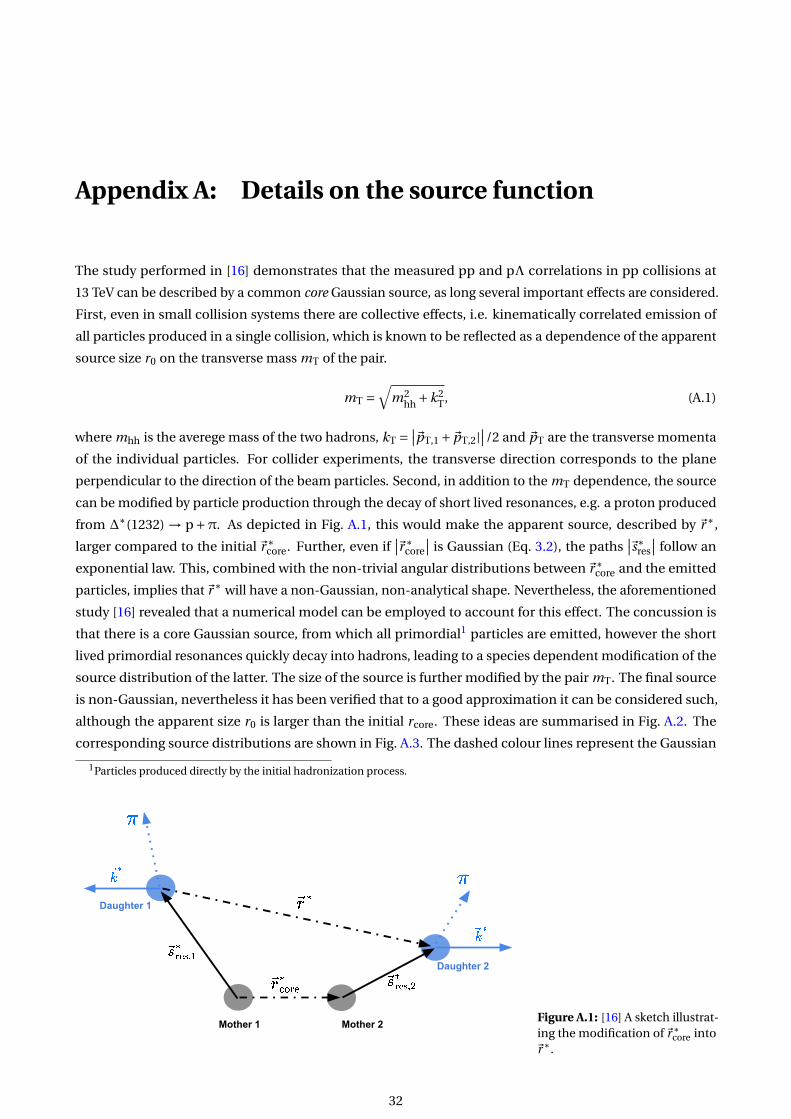
Appendix A: Details on the source function
The study performed in [16] demonstrates that the measured pp and pΛ correlations in pp collisions at
13 TeV can be described by a common core Gaussian source, as long several important effects are considered.
First, even in small collision systems there are collective effects, i.e. kinematically correlated emission of
all particles produced in a single collision, which is known to be reflected as a dependence of the apparent
source size r0 on the transverse mass mT of the pair.
mT =√
m2hh +k2
T, (A.1)
where mhh is the averege mass of the two hadrons, kT = ∣∣~pT,1 +~pT,2|∣∣/2 and ~pT are the transverse momenta
of the individual particles. For collider experiments, the transverse direction corresponds to the plane
perpendicular to the direction of the beam particles. Second, in addition to the mT dependence, the source
can be modified by particle production through the decay of short lived resonances, e.g. a proton produced
from ∆∗(1232) → p+π. As depicted in Fig. A.1, this would make the apparent source, described by ~r∗,
larger compared to the initial~r∗core. Further, even if
∣∣~r∗core
∣∣ is Gaussian (Eq. 3.2), the paths∣∣~s∗res
∣∣ follow an
exponential law. This, combined with the non-trivial angular distributions between~r∗core and the emitted
particles, implies that~r∗ will have a non-Gaussian, non-analytical shape. Nevertheless, the aforementioned
study [16] revealed that a numerical model can be employed to account for this effect. The concussion is
that there is a core Gaussian source, from which all primordial1 particles are emitted, however the short
lived primordial resonances quickly decay into hadrons, leading to a species dependent modification of the
source distribution of the latter. The size of the source is further modified by the pair mT. The final source
is non-Gaussian, nevertheless it has been verified that to a good approximation it can be considered such,
although the apparent size r0 is larger than the initial rcore. These ideas are summarised in Fig. A.2. The
corresponding source distributions are shown in Fig. A.3. The dashed colour lines represent the Gaussian
1Particles produced directly by the initial hadronization process.
Mother 1 Mother 2
Daughter 2
Daughter 1
Figure A.1: [16] A sketch illustrat-ing the modification of~r∗
core into~r∗.
32
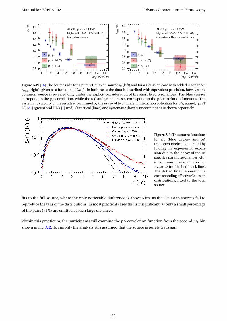
Manual for FOPRA 102 Advanced practicum in Femtoscopy
1 1.2 1.4 1.6 1.8 2 2.2 2.4 2.6)2c(GeV/⟩
Tm⟨
0.9
1
1.1
1.2
1.3
1.4
1.5
1.6(fm)
0r = 13 TeVsALICE pp 0)>% INEL0.17−High-mult. (0
Gaussian Source
p−p
(NLO)Λ−p
(LO)Λ−p
1 1.2 1.4 1.6 1.8 2 2.2 2.4 2.6)2c(GeV/⟩
Tm⟨
0.7
0.8
0.9
1
1.1
1.2
1.3
1.4(fm)
core
r
= 13 TeVsALICE pp 0)>% INEL0.17−High-mult. (0
Gaussian + Resonance Source
p−p
(NLO)Λ−p
(LO)Λ−p
Figure A.2: [16] The source radii for a purely Gaussian source r0 (left) and for a Gaussian core with added resonancesrcore (right), given as a function of ⟨mT⟩. In both cases the data is described with equivalent precision, however thecommon source is revealed only under the explicit consideration of the short lived resonances. The blue crossescorrepond to the pp correlation, while the red and green crosses correspond to the pΛ correlation functions. Thesystematic stability of the results is confirmed by the usage of two different interaction potentials for pΛ, namely χEFTLO [21] (green) and NLO [1] (red). Statistical (lines) and systematic (boxes) uncertainties are shown separately.
Figure A.3: The source functionsfor pp (blue circles) and pΛ(red open circles), generated byfolding the exponential expan-sion due to the decay of the re-spective parent resonances witha common Gaussian core ofrcore=1.2 fm (dashed black line).The dotted lines represent thecorresponding effective Gaussiandistributions, fitted to the totalsource.
fits to the full source, where the only noticeable difference is above 6 fm, as the Gaussian sources fail to
reproduce the tails of the distributions. In most practical cases this is insignificant, as only a small percentage
of the pairs (<1%) are emitted at such large distances.
Within this practicum, the participants will examine the pΛ correlation function from the second mT bin
shown in Fig. A.2. To simplify the analysis, it is assumed that the source is purely Gaussian.
33

Appendix B: ALICE experiment
Overview
The CERN complex is situated near Geneva, Switzerland, and hosts the largest accelerator complex existing
on the planet as of 2021. The largest machine is the Large Hadron Collider (LHC), designed to collide
protons and/or heavy ions at total collision energies of up to 14 TeV. One of the major experiments situated
at the LHC is ’A Large Ion Collider Experiment’ (ALICE), which had the original goal of concentrating on
heavy-ion collision physics, in particular the investigation of the quark gluon plasma phase by an accurate
determination of the species of the produced particles. This implies very good particle identification (PID)
capabilities. Nevertheless, these strengths can be used for the benefit of many physics studies, including
femtoscopy applied in pp collisions. The non-traditional femtoscopy group inside ALICE is often anecdotally
referring to the abbreviation of the experiment as ’A new Laboratory to Investigate and Constrain Exotic
hadron–hadron interactions’, due to the unique capabilities of the detector to perform such type of studies.
The experiment has 19 sub-detector systems, from which the most important one for tracking and PID is the
large Time Projection Chamber (TPC). Figure B.1 shows a schematic representation of ALICE. The limiting
Figure B.1: Schematic representation of the ALICE detector during the Run-2 data taking period (2015-2018) [22].
factor for ALICE is the low interaction and data read-out rates, the latter being limited to only ∼ 1 kHz, which
is 100 times lower compared to the ATLAS experiment. This is due to the ∼ 1 µs time span of reading out
a single event, during which the detector is not recording any further collisions. In the following a brief
summary of the detectors relevant for femtoscopy will be presented. The amount of data collected during
the second period of LHC operation (RUN2) in pp data corresponds to 109 of minimum-bias (MB) and
34
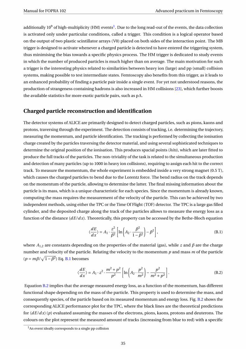
Manual for FOPRA 102 Advanced practicum in Femtoscopy
additionally 109 of high-multiplicity (HM) events1. Due to the long read-out of the events, the data collection
is activated only under particular conditions, called a trigger. This condition is a logical operator based
on the output of two plastic scintillator arrays (V0) placed on both sides of the interaction point. The MB
trigger is designed to activate whenever a charged particle is detected to have entered the triggering system,
thus minimising the bias towards a specific physics process. The HM trigger is dedicated to study events
in which the number of produced particles is much higher than on average. The main motivation for such
a trigger is the interesting physics related to similarities between heavy ion (large) and pp (small) collision
systems, making possible to test intermediate states. Femtoscopy also benefits from this trigger, as it leads to
an enhanced probability of finding a particle pair inside a single event. For yet not understood reasons, the
production of strangeness containing hadrons is also increased in HM collisions [23], which further boosts
the available statistics for more exotic particle pairs, such as pΛ.
Charged particle reconstruction and identification
The detector systems of ALICE are primarily designed to detect charged particles, such as pions, kaons and
protons, traversing through the experiment. The detection consists of tracking, i.e. determining the trajectory,
measuring the momentum, and particle identification. The tracking is performed by collecting the ionisation
charge created by the particles traversing the detector material, and using several sophisticated techniques to
determine the original position of the ionisation. This produces spacial points (hits), which are later fitted to
produce the full tracks of the particles. The non-triviality of the task is related to the simultaneous production
and detection of many particles (up to 1000 in heavy ion collisions), requiring to assign each hit to the correct
track. To measure the momentum, the whole experiment is embedded inside a very strong magnet (0.5 T),
which causes the charged particles to bend due to the Lorentz force. The bend radius on the track depends
on the momentum of the particle, allowing to determine the latter. The final missing information about the
particle is its mass, which is a unique characteristic for each species. Since the momentum is already known,
computing the mass requires the measurement of the velocity of the particle. This can be achieved by two
independent methods, using either the TPC or the Time Of Flight (TOF) detector. The TPC is a large gas filled
cylinder, and the deposited charge along the track of the particles allows to measure the energy loss as a
function of the distance (dE/d x). Theoretically, this property can be accessed by the Bethe-Bloch equation
⟨dE
d x⟩ = A1 · z2
β2
[ln
(A2 · β2
1−β2
)−β2
], (B.1)
where A1,2 are constants depending on the properties of the material (gas), while z and β are the charge
number and velocity of the particle. Relating the velocity to the momentum p and mass m of the particle
(p = mβ/√
1−β2) Eq. B.1 becomes
⟨dE
d x⟩ = A1 · z2 · m2 +p2
p2
[ln
(A2 · p2
m2
)− p2
m2 +p2
]. (B.2)
Equation B.2 implies that the average measured energy loss, as a function of the momentum, has different
functional shape depending on the mass of the particle. This property is used to determine the mass, and
consequently species, of the particle based on its measured momentum and energy loss. Fig. B.2 shows the
corresponding ALICE performance plot for the TPC, where the black lines are the theoretical predictions
for ⟨dE/d x⟩ (p) evaluated assuming the masses of the electrons, pions, kaons, protons and deuterons. The
colours on the plot represent the measured amount of tracks (increasing from blue to red) with a specific
1An event ideally corresponds to a single pp collision
35

Manual for FOPRA 102 Advanced practicum in Femtoscopy
Figure B.2: The energy loss as a function of momentum over charge, as measured by the ALICE TPC for pp collisions at13 TeV.
⟨dE/d x⟩ (p). The measured yield is clustered in several bands, each following the theoretical prediction of
a specific mass hypothesis, allowing the particle identification. The width (σ) of each band is related to
the resolution of the TPC. To determine the best mass hypothesis each particle is assigned a nσ parameter
measuring the discrepancy in number of σ (resolution) between the theoretical expectation to measure
⟨dE/d x⟩ (p) for a given particle species and the measured value. At small momenta (below c.a. 1 GeV/c) the
individual particles (bands) are separated quite well, however at larger momenta the resolution becomes
insufficient to perform the PID. This issue can be addressed by using complementary information from other
detectors, such as the TOF. This detector provides a measurement of the time difference between the initial
collision and a particle reaching it. The detector is at a fixed position, thus the timing information allows to
evaluate the velocity and consequently the mass.
β= p√m2 +p2
. (B.3)
Similarly to the Bethe-Bloch relation, Eq. B.3 can be used to plot the expected relation for a fixed mass,
as shown in Fig. B.3. Using the TOF detector allows to separate the particle to much larger momentum
range, compared to the TPC. Since the TOF is located further away from the collision point, the particles
have a lower probability of reaching it, as they might be absorbed within the detector systems they have to
traverse, or bent back by the magnetic field in case of low momentum particles. This significantly reduces
the reconstruction efficiency (the detected number of particles). For that reason, in femtoscopy the TPC is
the only detector deployed to detect particles below c.a. 1 GeV/c, while for the rest the supplementary TOF
information is included, achieving a good balance between yield and purity.
Reconstruction ofΛ particles
The Λ baryon (uds) is a weakly decaying state (Λ→ pπ−). The decay length is around 7.9 cm, which is
much smaller than the c.a. 80 cm inner radius of the TPC. This implies that most of theΛs produced in the
collision will decay before they have reached the TPC, allowing to measure the charged daughters. Their
36

Manual for FOPRA 102 Advanced practicum in Femtoscopy
Figure B.3: Particle identification using the Time-Of-Flight detector.
Figure B.4: Invariant mass ofΛ candidates with k∗ below24 MeV/c , and the correspondingfits. The fits use several differenthypothesis to decompose the sig-nal and the background, in orderto evaluate the systematic uncer-tainties (c.a. 1%).
invariant mass, evaluated from their four vectors, should correspond to the mass of theΛ (MΛ = 1116 MeV).
By building the invariant mass spectrum of the measured pπ− and selecting only those close to the expected
Λ mass, the Λ baryon can be reconstructed. Naturally, uncorrelated pπ− pairs may have, by chance, an
invariant mass similar to MΛ, leading to falsely identified candidates. Nevertheless, using several appropriate
topological conditions it is possible to reduce this effect, leading to very pure invariant mass spectrum. In
the present analysis, theΛ purity is ∈ (95,96)%, which is extracted from the spectrum plotted in Fig. B.4.
37

Bibliography
A useful hint: if a reference is not with an open access, most of the time there is a ’beta’ version with the
same title on https://arxiv.org/, you just need to search for it. Another good search platform, dedicated to
high-energy physics, is https://inspirehep.net/. It typically provides a link to the arXiv version of each paper.
[1] J. Haidenbauer, S. Petschauer, N. Kaiser, U.-G. Meissner, A. Nogga, and W. Weise.
Hyperon-nucleon interaction at next-to-leading order in chiral effective field theory.
Nucl. Phys. A, 915:24–58, 2013. doi: 10.1016/j.nuclphysa.2013.06.008.
[2] D. R. Entem, R. Machleidt, and Y. Nosyk.
High-quality two-nucleon potentials up to fifth order of the chiral expansion.
Phys. Rev. C, 96(2):024004, 2017. doi: 10.1103/PhysRevC.96.024004.
[3] David Griffiths.
Introduction to Quantum Mechanics.
Pearson Prentice Hall, 2004. ISBN 978-1107179868.
[4] J. J. Sakurai and Jim Napolitano.
Modern Quantum Mechanics.
Pearson Education Limited, 2014. ISBN 978-1-292-02410-3.
[5] G. Alexander, U. Karshon, A. Shapira, G. Yekutieli, R. Engelmann, H. Filthuth, and W. Lughofer.
Study of the lambda-n system in low-energy lambda-p elastic scattering.
Phys. Rev., 173:1452–1460, 1968. doi: 10.1103/PhysRev.173.1452.
[6] B. Sechi-Zorn, B. Kehoe, J. Twitty, and R. A. Burnstein.
Low-energy lambda-proton elastic scattering.
Phys. Rev., 175:1735–1740, 1968. doi: 10.1103/PhysRev.175.1735.
[7] J. A. Kadyk, G. Alexander, J. H. Chan, P. Gaposchkin, and G. H. Trilling.
Lambda p interactions in momentum range 300 to 1500 mev/c.
Nucl. Phys. B, 27:13–22, 1971. doi: 10.1016/0550-3213(71)90076-9.
[8] H. Takahashi et al.
Observation of a (Lambda Lambda)He-6 double hypernucleus.
Phys. Rev. Lett., 87:212502, 2001. doi: 10.1103/PhysRevLett.87.212502.
[9] Emiko Hiyama and Kazuma Nakazawa.
Structure of S=-2 Hypernuclei and Hyperon-Hyperon Interactions.
Ann. Rev. Nucl. Part. Sci., 68:131–159, 2018. doi: 10.1146/annurev-nucl-101917-021108.
[10] Diego Lonardoni, Alessandro Lovato, Stefano Gandolfi, and Francesco Pederiva.
Hyperon Puzzle: Hints from Quantum Monte Carlo Calculations.
Phys. Rev. Lett., 114(9):092301, 2015. doi: 10.1103/PhysRevLett.114.092301.
38

Manual for FOPRA 102 Advanced practicum in Femtoscopy
[11] Paul Demorest, Tim Pennucci, Scott Ransom, Mallory Roberts, and Jason Hessels.
Shapiro Delay Measurement of A Two Solar Mass Neutron Star.
Nature, 467:1081–1083, 2010. doi: 10.1038/nature09466.
[12] John Antoniadis et al.
A Massive Pulsar in a Compact Relativistic Binary.
Science, 340:6131, 2013. doi: 10.1126/science.1233232.
[13] H. T. Cromartie et al.
Relativistic Shapiro delay measurements of an extremely massive millisecond pulsar.
Nature Astron., 4(1):72–76, 2019. doi: 10.1038/s41550-019-0880-2.
[14] Michael Annan Lisa, Scott Pratt, Ron Soltz, and Urs Wiedemann.
FEMTOSCOPY IN RELATIVISTIC HEAVY ION COLLISIONS: Two Decades of Progress.
Annual Review of Nuclear and Particle Science, 55(1):357–402, 2005. doi: 10.1146/annurev.nucl.55.
090704.151533.
[15] ALICE Collaboration.
p-p, p-Λ andΛ-Λ correlations studied via femtoscopy in pp reactions atp
s = 7 TeV.
Phys. Rev. C, 99(2):024001, 2019. doi: 10.1103/PhysRevC.99.024001.
[16] ALICE Collaboration.
Search for a common baryon source in high-multiplicity pp collisions at the LHC.
Physics Letters B, 811:135849, 2020. doi: 10.1016/j.physletb.2020.135849.
[17] D.L. Mihaylov, V. Mantovani Sarti, O.W. Arnold, L. Fabbietti, B. Hohlweger, and A.M. Mathis.
A femtoscopic Correlation Analysis Tool using the Schrödinger equation (CATS).
Eur. Phys. J. C, 78(5):394, 2018. doi: 10.1140/epjc/s10052-018-5859-0.
[18] R. Lednicky and V.L. Lyuboshits.
Final State Interaction Effect on Pairing Correlations Between Particles with Small Relative Momenta.
Sov. J. Nucl. Phys., 35:770, 1982.
[19] R. Brun and F. Rademakers.
ROOT: An object oriented data analysis framework.
Nucl. Instrum. Meth. A, 389:81–86, 1997. doi: 10.1016/S0168-9002(97)00048-X.
[20] William H. Press, Saul A. Teukolsky, William T. Vetterling, and Brian P. Flannery.
Numerical Recipes 3rd Edition: The Art of Scientific Computing, chapter 15.6.1.
Cambridge University Press, New York, NY, USA, 3 edition, 2007. ISBN 0521880688, 9780521880688.
[21] Henk Polinder, Johann Haidenbauer, and Ulf-G. Meissner.
Hyperon-nucleon interactions: A Chiral effective field theory approach.
Nucl. Phys. A, 779:244–266, 2006. doi: 10.1016/j.nuclphysa.2006.09.006.
[22] ALICE Collaboration.
ALICE Figure repository.
Accessed 4th December 2020.
[23] ALICE Collaboration.
Enhanced production of multi-strange hadrons in high-multiplicity proton-proton collisions.
Nature Phys., 13:535–539, 2017. doi: 10.1038/nphys4111.
39
Top Related