


Languages
Pages
Legal

Adaptive MIMO Radar
Luzhou Xu 1, Jian Li 1, Petre Stoica 2
Abstract
We investigate several adaptive techniques for a multiple-input multiple-output (MIMO)
radar system (that is, a radar with multiple transmitting and receiving antennas). By
transmitting independent waveforms via different antennas, the echoes due to targets at
different locations are linearly independent of each other, which allows the direct appli-
cation of many adaptive techniques to achieve high resolution and excellent interference
rejection capability. In the absence of array steering vector errors, we discuss the applica-
tion of several existing adaptive algorithms including Capon, APES (amplitude and phase
estimation) and CAPES (combined Capon and APES), and then propose an alternative
estimation procedure, referred to as the combined Capon and approximate maximum like-
lihood (CAML) method. Via several numerical examples, we show that the proposed
CAML method can provide excellent estimation accuracy of both target locations and
target amplitudes. In the presence of array steering vector errors, we apply the robust
Capon beamformer (RCB) and doubly constrained robust Capon beamformer (DCRCB)
approaches to the MIMO radar system to achieve accurate parameter estimation and
superior interference and jamming suppression performance.
Index Terms – Adaptive arrays, MIMO Radar, direction of arrival (DOA), Capon, ampli-
tude and phase estimation (APES), robust Capon beamformer (RCB), doubly constrained
robust Capon beamformer (DCRCB).
IEEE TRANSACTIONS ON AEROSPACE AND ELECTRONIC SYSTEMS 3
Submitted in April 2006
1Luzhou Xu and Jian Li are with the Department of Electrical and Computer Engineering, University of Florida,
Gainesville, USA.2Petre Stoica is with the Department of Information Technology, Uppsala University, Uppsala, Sweden.3Please address all correspondences to: Dr. Jian Li, the Department of Electrical and Computer Engineering,
P. O. Box 116130, University of Florida, Gainesville, USA. Phone: (352) 392-2642, Fax: (352) 392-0044, Email:
I. Introduction
A MIMO (multiple-input multiple-output) radar uses multiple antennas to simultane-
ously transmit several (possibly linearly independent) waveforms and it also uses multiple
antennas to receive the reflected signals [1] [2] [3] [4] [5] [6] [7] [8]. The statistical MIMO
radar, proposed in [2], [3] and [4], is different from the conventional radar systems in that
the signal “fading” effect due to the target’s scintillations, which can cause severe perfor-
mance degradations, is mitigated via the use of a new radar architecture and the spacing
between the adjacent elements of the array is large to achieve the diversity gain. In [5],
a transmitting beamforming approach, using partial signal correlation, is proposed and it
is shown that a desired transmitting beampattern can be achieved or approximated via
choosing the correlation matrix of the waveforms. In [6], a MIMO radar technology is
suggested to improve the radar resolution. The idea is to transmit N (N > 1) orthogo-
nal coded waveforms by N antennas and to receive the reflected signals by M (M > 1)
antennas. At each receiving antenna output, the signal is matched-filtered using each of
the transmitted waveforms to obtain NM channels, to which the data-adaptive Capon
beamformer [9] is applied. It is proved in [6] that the beampattern of the proposed MIMO
radar is obtained by the multiplication of the transmitting and receiving beampatterns,
which gives high resolution. However, the derivation of the proposed method in [6] and its
theoretical performance analysis are valid only in the single target case. When there are
multiple targets, the problem in [6] turns out to be a coherent-source problem, in which
case Capon and many other adaptive methods fail to work properly. Specifically, the
equation of the signal covariance (see Equation (7) in [6]), on which the Capon algorithm
relies, is no longer valid. Moreover, the distributive law of the Khatri-Rao product used
1
in the performance analysis in [6] (see Equations (9) and (10) in [6]) is no longer valid in
the presence of multiple targets.
We consider herein a new MIMO radar scheme that can deal with multiple targets. In
this paper, we focus on the narrow-band MIMO radar. Similar to some of the aforemen-
tioned MIMO radar approaches, linearly independent waveforms are transmitted simul-
taneously via multiple antennas. Due to the different phase shifts associated with the
different propagation paths from the transmitting antennas to targets, these independent
waveforms are linearly combined at the targets with different phase factors. As a result,
the signal waveforms reflected from different targets are linearly independent of each other,
which allows for the application of Capon and of other adaptive array algorithms. We con-
sider applying two well-known adaptive approaches, i.e., the Capon and APES (Amplitude
and Phase Estimation) [10] algorithms, to the proposed MIMO radar system to estimate
the target locations and the reflected signal amplitudes. We show via numerical examples
that Capon can provide accurate estimates of the target locations, while its amplitude
estimates are biased downward. APES gives accurate amplitude estimates at the cost of
poorer resolution and hence poorer estimation accuracy of target locations. To exploit the
merits of both Capon and APES, we consider a combined method, referred to as CAPES
[11], which first estimates the target locations using the Capon method and then refines
the amplitude estimates at the estimated locations using the APES estimator. To further
improve the amplitude estimation accuracy, we combine Capon and an approximate max-
imum likelihood (AML) method recently introduced in [12]. We refer to the so-obtained
method as CAML. In CAML, the AML estimator, which is devised in [12] based on a
diagonal growth curve (DGC) model, is used to replace APES in CAPES. As shown in
2
Section V, this new method can provide higher amplitude estimation accuracy than that
of the existing methods.
We also investigate robust adaptive methods in the presence of array calibration errors.
It is well-known that the performance of Capon degrades severely in the presence of steering
vector errors. This problem also affects APES and other adaptive methods, but to a lesser
extent. In the presence of array calibration errors, we suggest the use of the recently
proposed robust Capon beamformer (RCB) (see [13], [14] and references therein) and the
doubly constrained robust Capon beamformer (DCRCB) [15] to process the MIMO radar
data. As shown in the numerical examples, when array calibration errors are present, RCB
and DCRCB significantly outperform the aforementioned (non-robust) adaptive methods.
The remainder of this paper is organized as follows. In Section II, we describe our
MIMO radar scheme and the associated data model. Several adaptive methods and two
robust adaptive methods are presented in Sections III and IV, respectively. We provide
several numerical examples in Section V. Finally, Section VI contains our conclusions.
II. Signal Model
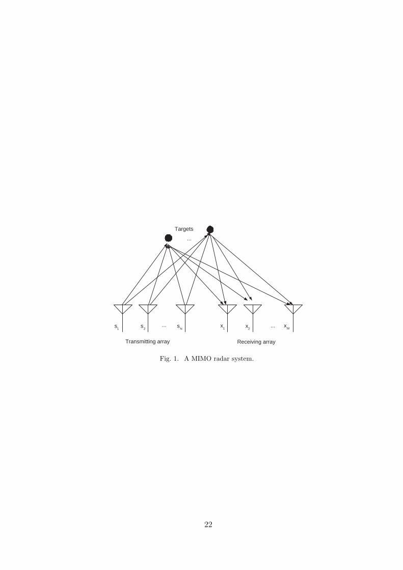
Consider a MIMO narrowband radar system with N arbitrarily located transmitting
antennas and M arbitrarily located receiving antennas as shown in Fig. 1 4. The system
simultaneously transmits N linearly independent waveforms, denoted by sn ∈ CL×1 (n =
1, 2, · · ·N) with L being the snapshot number. Let θ be the location parameter of a
generic target, for example, the direction of arrival (DOA) when the targets are in the far
4Note that in Fig. 1, we have separated the transmitting array from the receiving array for the sake of generality.
However, in practical applications, the two sub-arrays may have many common elements. Also, the targets in Fig.
1 are in the near field for illustration purposes only. In practice, the targets can be in the far field.
3
field of the arrays 5, and let at(θ) be the corresponding steering vector for the transmitting
antenna array. Then the waveform vector of the reflected signals from the target at θ is
aTt (θ)S with (·)T denoting the transpose and S = [s1 s2 · · · sN ]T . Note that aT
t (θ)S is a
function of the location parameter θ. Hence, the signals reflected from targets at different
locations are linearly independent of each other. By assuming that the targets are located
in the same range bin, the reflected signals arrive at the receiving array at about the same
time and the arrival time is known.
The signal matrix at the output of the receiving array has the form:
X = ar(θ)β(θ)aTt (θ)S + Z, (1)
where the columns of X ∈ CM×L are the received data snapshots, ar(θ) ∈ CM×1 is the
steering vector of the receiving antenna array and β(θ) ∈ C denotes the complex amplitude
of the reflected signal from θ, i.e., the “reflection coefficient” of the focal point θ. The
matrix Z ∈ CM×L denotes the residual term, which includes the unmodelled noise, inter-
ferences from targets at locations other than θ, and intentional or unintentional jamming.
For notional simplicity, we will not show explicitly the dependence of Z on θ.
The problem is to estimate β(θ) for each θ of interest from the observed data matrix
X. The estimates of {β(θ)} can be used to form a spatial spectrum in the 1D case or a
radar image in the 2D case. We can then estimate the locations of the targets and their
“reflection coefficients” by searching for the peaks in the so-obtained spectrum (or image).
5Note that when the transmitting and receiving arrays are different, the DOAs for the two arrays are different.
Since we know the relative positions of the two arrays, we can use the same DOA variable for notational convenience.
4
III. Adaptive Approaches in the Absence of Array Calibration Errors
A simple way to estimate β(θ) in (1) is via the Least Squares (LS) method:
βLS(θ) =aH
r (θ)XSH a∗t (θ)
L ‖ ar(θ) ‖2 [aTt (θ)RSSa∗t (θ)]
(2)
where (·)H and (·)∗ denote the conjugate transpose and the complex conjugate, respec-
tively, ‖ · ‖ denotes the Euclidean norm, and
RSS =1
LSSH (3)
is the correlation matrix of the waveforms. However, as any other data-independent
beamforming-type method, the LS method suffers from high sidelobes and low resolu-
tion. In the presence of strong interference and jamming, this method completely fails to
work.
We present below several adaptive beamforming-based methods, which, as shown via nu-
merical examples in Section V, have much higher resolution and much better interference-
rejection capability than the LS method.
A. Capon
The Capon estimator consists of two main steps. The first is the Capon beamforming
step [9] [16]. The second is a LS estimation step, which involves basically a matched
filtering.
The Capon beamformer can be formulated as follows:
minw
wHRw subject to wHar(θ) = 1, (4)
where w ∈ CM×1 is the weight vector used to achieve noise, interference and jamming
suppression while keeping the desired signal undistorted, and R is the sample covariance
5
of the observed snapshots, i.e.,
R =1
LXXH . (5)
Following [9] and [16], we can readily obtain the solution to (4) as:
wcapon =R−1ar(θ)
aHr (θ)R−1ar(θ)
, (6)
The output of the Capon beamformer is thus given by
aHr (θ)R−1X
aHr (θ)R−1ar(θ)
. (7)
Substituting (1) into (7) yields
aHr (θ)R−1X
aHr (θ)R−1ar(θ)
= β(θ)aTt (θ)S +
aHr (θ)R−1Z
aHr (θ)R−1ar(θ)
. (8)
Applying the LS method to (8), we get the Capon estimate of β(θ) as follows:
βCapon(θ) =aH
r (θ) R−1XSH a∗t (θ)
L [aHr (θ)R−1ar(θ)][aT
t (θ)RSSa∗t (θ)], (9)
where RSS is defined in (3).
B. APES
The Amplitude and Phase Estimation (APES) approach [10] [17] [18] is a non-parametric
spectral analysis method with superior estimation accuracy [19] [20]. We apply this method
to the proposed MIMO radar system to achieve better amplitude estimation accuracy.
By following [17], the APES method can be formulated as:
minw,β
‖ wHX− β(θ)aTt (θ)S ‖2 subject to wHar(θ) = 1, (10)
where w ∈ CM×1 is the weight vector. Intuitively, the goal of (10) is to find a beamformer
whose output is as close as possible to a signal with the waveform given by aTt (θ)S.
6
Minimizing the cost function in (10) with respect to β(θ) yields
βAPES(θ) =wHXSHa∗t (θ)
L aTt (θ)RSSa∗t (θ)
. (11)
Then the optimization problem in (10) reduces to
minw
wHQw subject to wHar(θ) = 1 (12)
with
Q = R− XSH a∗t (θ)aTt (θ)SXH
L2 aTt (θ)RSSa∗t (θ)
. (13)
Solving the optimization problem in (12) gives the APES beamformer weight vector [17]:
wAPES =Q−1ar(θ)
aHr (θ)Q−1ar(θ)
. (14)
By inserting (14) into (11), the APES estimate of β(θ) is readily obtained as:
βAPES(θ) =aH
r (θ)Q−1XSH a∗t (θ)
L [aHr (θ)Q−1ar(θ)] [aT
t (θ)RSSa∗t (θ)]. (15)
Note that the only difference between the Capon estimator and the APES estimator is
that the sample covariance matrix R in (9) is replaced in (15) by the residual covariance
estimate Q. However, this seemingly minor difference makes these two methods behave
quite differently (see, e.g., Section V).
C. CAPES and CAML
As discussed in [10] (see also Section V), the above two adaptive methods behave dif-
ferently. Capon has high resolution, and hence can provide accurate estimates of the
target locations. However, the Capon amplitude estimates are significantly biased down-
ward. The APES estimator gives much more accurate amplitude estimates at the target
locations, but at the cost of lower resolution.
7
To reap the benefits of both Capon and APES, an alternative estimation procedure,
referred to as CAPES, is proposed in [11]. CAPES first estimates the peak locations using
the Capon estimator and then refines the amplitude estimates at these locations using the
APES estimator. CAPES can be directly applied to the MIMO radar target localization
and amplitude estimation problem considered herein.
Inspired by the CAPES method, we propose below a new approach, referred to as
CAML, which combines Capon and the recently proposed approximate maximum likeli-
hood (AML) estimator based on a diagonal growth curve (DGC) model [12]. In CAML,
AML, instead of APES, is used to estimate the target amplitudes at the target locations
estimated by Capon. Since, unlike APES, AML estimates the amplitudes of all targets at
given locations jointly rather than one at a time, the latter can provide better estimation
accuracy than the former.
Let θk (k = 1, 2, · · ·K) denote the estimated target locations, i.e., the peak locations of
the spatial spectrum estimated by Capon. Here K is assumed known. If K is unknown, it
can be determined accurately using a generalized likelihood ratio test (GLRT), the details
of which are given in the Appendix. Let
Ar = [ar(θ1) ar(θ2) · · · ar(θK)], (16)
At = [at(θ1) at(θ2) · · · at(θK)], (17)
and
β = [β(θ1) β(θ2) · · · β(θK)]T . (18)
Then the data model in (1) can be re-formulated as a DGC model [12]:
X = ArB(ATt S) + Z with B = diag(β), (19)
8
where diag(β) denotes a diagonal matrix whose diagonal elements are equal to the elements
of β, and Z is the residual term. Since the maximum likelihood (ML) estimate of β in
(19) cannot be produced in closed-form, we use the AML estimator in [12] instead, which
is asymptotically equivalent to the ML for a large snapshot number L.
By using the AML method in Equation (18) of [12], the estimate of β can be readily
obtained as:
βAML =1
L[(AH
r T−1Ar)¯ (AHt R∗
SSAt)]−1 vecd(AH
r T−1XSHA∗t ), (20)
where ¯ denotes the Hadamard product [21], vecd(·) denotes a column vector formed by
the diagonal elements of a matrix, and
T = L R− 1
LXSHA∗
t (ATt RSSA
∗t )−1AT
t SXH . (21)
IV. Adaptive Approaches in the Presence of Array Calibration Errors
The previous adaptive methods assume that the transmitting and receiving arrays are
perfectly calibrated, i.e., at(θ) and ar(θ) are accurately known as functions of θ. However,
in practice, array calibration errors are often inevitable. The presence of array calibration
errors and the related small snapshot number problem [22] can degrade significantly the
performance of the adaptive methods discussed so far.
A. RCB
We consider the application of the robust Capon beamformer (RCB) ( see [13], [14] and
references therein) to a MIMO radar system that suffers from calibration errors. RCB
allows ar(θ) to lie in an uncertainty set. Without loss of generality, we assume that ar(θ)
9
belongs to an uncertainty sphere:
‖ ar(θ)− ar(θ) ‖2≤ ε (22)
with both ar(θ), the nominal receiving array steering vector, and ε being given. (For the
more general case of ellipsoidal uncertainty sets, see [13], [14] and references therein.) Note
that the calibration errors in at(θ) will also degrade the accuracy of the estimate of β(θ)
(see (9)). However, the LS (or matched filtering) approach of (9) is quite robust against
calibration errors in at(θ).
The RCB method is based on the following covariance fitting formulation [13] [14] [23]:
maxσ2(θ),ar(θ)
σ2(θ) subject to R− σ2(θ)ar(θ)aHr (θ) ≥ 0
‖ ar(θ)− ar(θ) ‖2≤ ε,
(23)
where σ2(θ) denotes the power of the signal of interest and P ≥ 0 means that P is
Hermitian positive semi-definite. The optimization problem in (23) can be simplified as
[13]:
minar(θ)
aHr (θ)R−1ar(θ) subject to ‖ ar(θ)− ar(θ) ‖2≤ ε. (24)
By using the Lagrange multiplier methodology [13], the solution to (24) is found to be
ar(θ) = ar(θ)− [I + λ(θ)R]−1ar(θ), (25)
where I denotes the identity matrix. The Lagrange multiplier λ(θ) ≥ 0 in (25) is obtained
as the solution to the constraint equation
‖ [I + λ(θ)R]−1 ar(θ) ‖2= ε, (26)
which can be solved efficiently by using the Newton method since the left side of (26) is a
monotonically decreasing function of λ(θ) (see [13] for more details). Once the Lagrange
10
multiplier λ(θ) is determined, ar(θ) is obtained from (25). To eliminate a scaling ambiguity
(see [13]), we scale ar(θ) such that ‖ ar(θ) ‖2= M . Replacing ar(θ) in (9) by the scaled
steering vector ar(θ) yields the RCB estimate of β(θ).
B. DCRCB
A doubly constrained robust Capon beamformer (DCRCB) is proposed in [15]. In
the DCRCB, in addition to the spherical constraint in (22), the steering vector ar(θ) is
constrained to have a constant norm, i.e.,
‖ ar(θ) ‖2= M. (27)
Then the covariance fitting formulation (see (23)) becomes:
maxσ2(θ),ar(θ)
σ2(θ) subject to R− σ2(θ)ar(θ)aHr (θ) ≥ 0
‖ ar(θ)− ar(θ) ‖2≤ ε
‖ ar(θ) ‖2= M.
(28)
The optimization problem in (28) can be simplified to [15]:
minar(θ)
aHr (θ)R−1ar(θ) subject to Re[aH
r (θ)ar(θ)] ≥ M − ε
2
‖ ar(θ) ‖2= M,
(29)
where Re(·) denotes the real part of a complex number. Let u1 be the principal eigenvector
of R, and let
ar(θ) = M12 u1 exp
{j arg
[uH
1 ar(θ)]}
(30)
with arg(·) denoting the phase of a complex number. If ar(θ) in (30) satisfies
Re[ aHr (θ)ar(θ) ] ≥ M − ε
2, (31)
11
then, obviously, ˆar(θ) = ar(θ) is the optimal solution of (29). Otherwise, by using the
Lagrange multiplier methodology [15], the optimal solution to (29) is
ˆar(θ) =(M − ε
2
) [R−1 + λ(θ)I]−1 ar(θ)
aHr (θ) [R−1 + λ(θ)I]−1 ar(θ)
. (32)
The Lagrange multiplier λ(θ) in (32), which can be negative, is obtained as the solution
to the constraint equation
aHr (θ) [R−1 + λ(θ)I]−2 ar(θ){
aHr (θ) [R−1 + λ(θ)I]−1 ar(θ)
}2 =M
(M − ε2)2
. (33)
Like in the case of RCB, the constraint equation (33) can be solved efficiently by using
the Newton method since the left side of (33) is a monotonically decreasing function of
λ(θ) (see [15] for more details).
We summarize the DCRCB estimator of β(θ) as follows:
1. Compute ar(θ) by (30).
2. If ar(θ) satisfies (31), estimate β(θ) by replacing ar(θ) in (9) by ˆar(θ) = ar(θ), and
stop.
3. If (31) is not satisfied, solve (33) for λ(θ). Calculate ˆar(θ) by (32) using the so-obtained
λ(θ).
4. Compute the DCRCB estimate of β(θ) by replacing ar(θ) in (9) by ˆar(θ), and stop.
V. Numerical Examples
Consider a MIMO radar system where a uniform linear array with N = M = 10 antennas
and half-wavelength spacing between adjacent antennas is used both for transmitting and
for receiving. The transmitted waveforms sn (n = 1, 2, · · · N) are orthogonal quadrature
phase shift keyed (QPSK) sequences, and hence we have RSS = I (this choice of Rss is
12
optimal in a maximum-SNR sense, see [24]).
Consider a scenario in which K = 3 targets are located at θ1 = −40◦, θ2 = −25◦, and
θ3 = −10◦ with “reflection coefficients” β1 = 4, β2 = 4, and β3 = 1, respectively. There is
a strong jammer at 0◦ with an unknown waveform and with amplitude 1000, i.e., 60 dB
above β3. The received signal has L = 256 snapshots and is corrupted by a zero-mean
spatially colored Gaussian noise with an unknown covariance matrix. The (p, q)th element
of the unknown noise covariance matrix is 1
SNR 0.9|p−q|ej(p−q)π
2 .
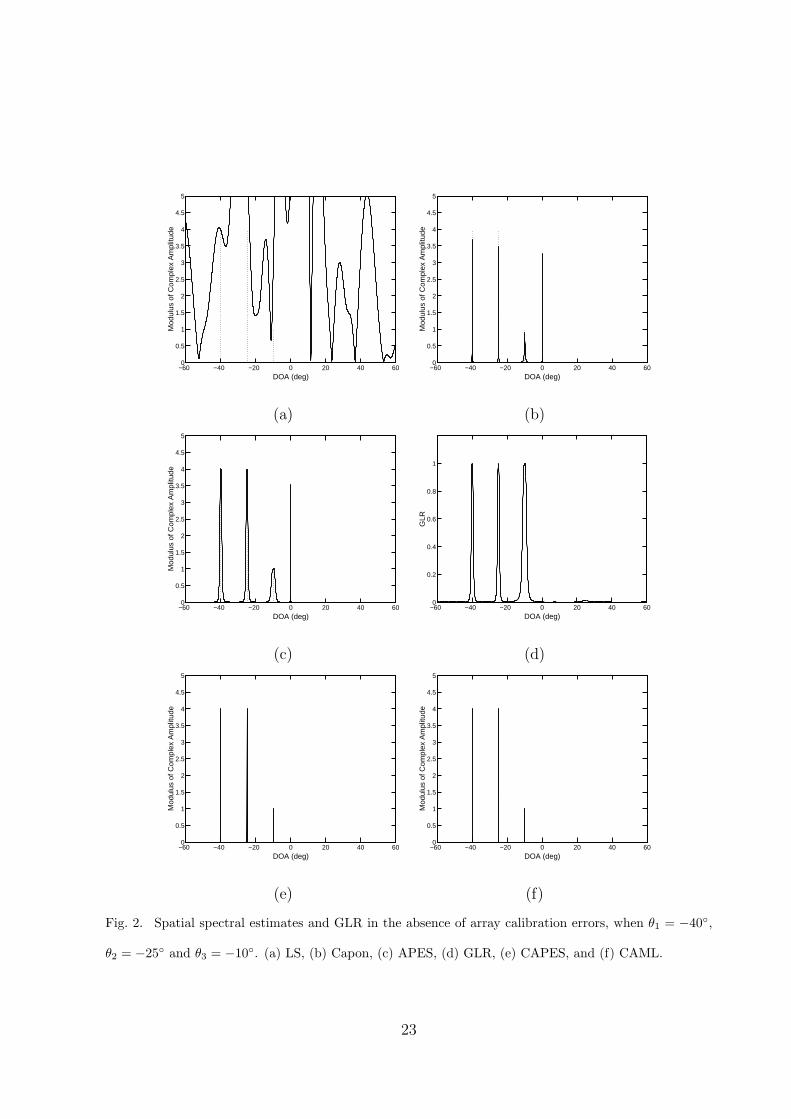
We first consider the case of no array calibration errors. Let SNR = 10 dB. The moduli
of the spatial spectral estimates of β(θ), versus θ, obtained by using LS, Capon, APES,
CAPES and CAML are given in Figs. 2(a), (b), (c), (e) and (f), respectively. For com-
parison purpose, we also show the true spatial spectrum via dashed lines in these figures.
As seen in Fig. 2(a), the LS method suffers from high sidelobes and low resolution. Due
to the presence of the strong jamming signal, the LS estimator fails to work properly.
Capon and APES possess great interference and jamming suppression capabilities. The
Capon method gives very narrow peaks around the target locations. However, the Capon
amplitude estimates are biased downward. The APES method gives more accurate am-
plitude estimates around the target locations but its resolution is slightly worse than that
of Capon. Note that in Figs. 2(a)-2(c) a false peak occurs at θ = 0◦ due to the presence
of the strong jammer. Despite the fact that the jammer waveform is statistically indepen-
dent of the waveforms transmitted by the MIMO radar, a false peak still exists since the
jammer is 60 dB stronger than the weakest target and the snapshot number is finite.
To reject the false peak, we use a generalized likelihood ratio test (GLRT) for each angle
13
of interest; the GLR is given by (see the Appendix for details):
ρ(θ) = 1− aHr (θ)R−1ar(θ)
aHr (θ)Q−1ar(θ)
, (34)
where R and Q are given in (5) and (13), respectively. Fig. 2 (d) gives the GLR as a
function of the target location parameter θ. As expected, we get high GLRs at the target
locations and low GLRs at other locations including the jammer location. By comparing
the GLR with a threshold, the false peak due to the strong jammer can be readily detected
and rejected, and a correct estimate of the number of the targets can be obtained. This
information can be passed to CAPES and CAML to obtain Figs. 2(e) and 2(f). As seen
from these figures, both CAPES and CAML give accurate estimates of the target locations
and amplitudes.
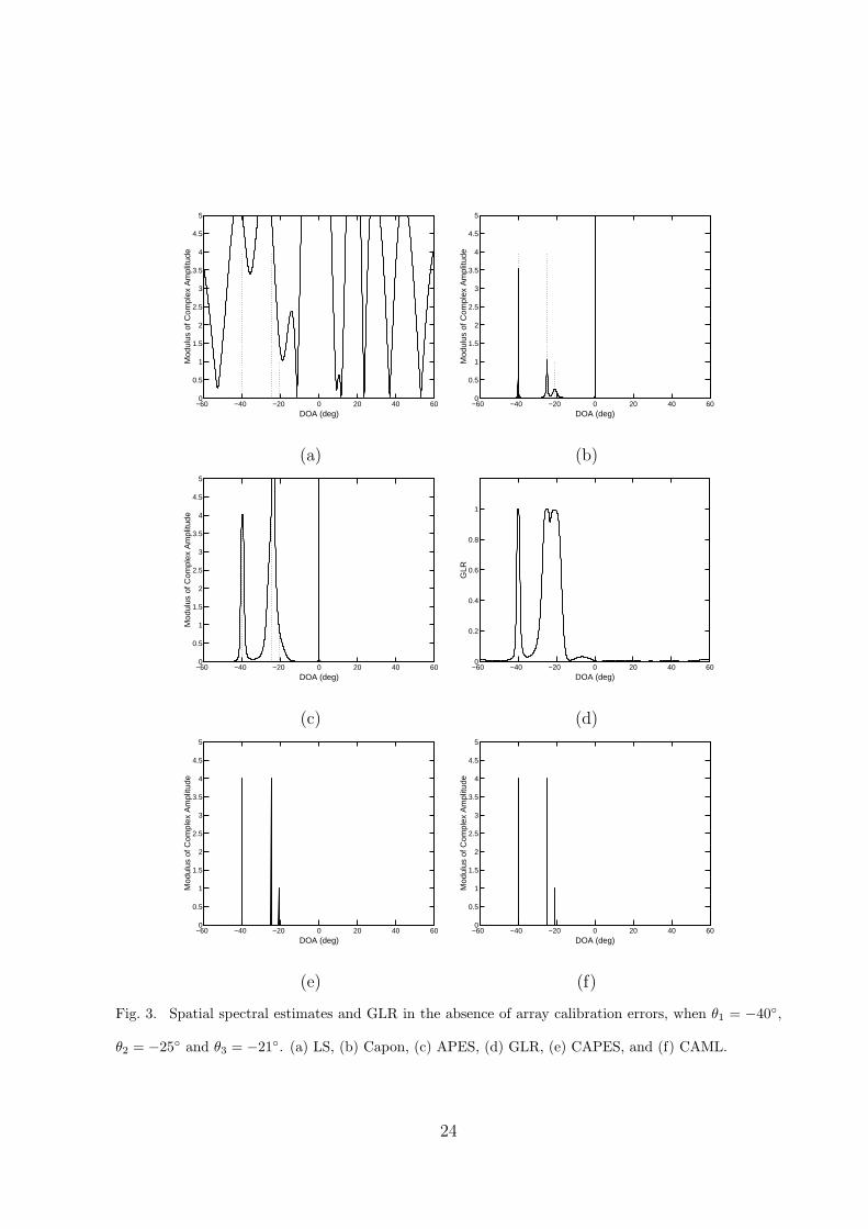
Next we consider a more challenging example where θ3 is −21◦ while all the other
simulation parameters are the same as before. As shown in Fig. 3(c), in this example the
APES method fails to resolve the two closely spaced targets at θ2 = −25◦ and θ3 = −21◦.
On the other hand, Capon gives well-resolved peaks around the target locations, but its
amplitude estimates are significantly biased downward. Based on the GLR in Fig. 3(d),
the false peak due to the strong jammer can be readily rejected. Once again CAPES
and CAML outperform the other methods and provide quite accurate target parameter
estimates.
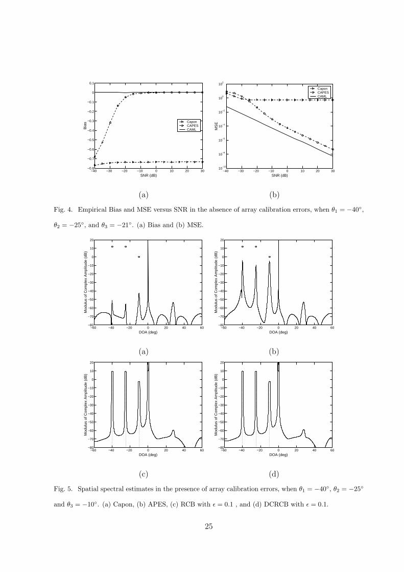
To illustrate the improvement of CAML over CAPES for target amplitude estimation,
we consider the amplitude estimation performance of Capon, CAPES, and CAML as a
function of SNR. All the other simulation parameters are the same as in Fig. 3. Figs.
4(a) and 4(b) show, respectively, the bias and mean-squared error (MSE) of the amplitude
14
estimate for the target at θ3. The results are obtained using 1000 Monte-Carlo simulations.
As seen from these figures, the Capon estimate is biased downward significantly. Due to
this bias, an error floor occurs in the MSE of the Capon estimate. CAPES is also biased
downward at very low SNR. The CAML estimator is unbiased and outperforms CAPES
for the entire range of the SNR considered, especially at low SNR.
We next consider the case where array calibration errors are present. To simulate the
array calibration error, each element of the steering vector at(θ) = ar(θ), for each incident
signal, is perturbed with a zero-mean circularly symmetric complex Gaussian random
variable with variance 0.005 and then scaled to have norm√
M , so that the squared
Euclidean norm of the difference between the true array steering vector and the presumed
one is about 0.05. We let SNR = 30 dB. The other simulation parameters are the same
as those in Fig. 2. For the sake of description convenience, the moduli of the amplitude
estimates, i.e., the y-axes of Figs. 5(a)-5(d), are on a dB scale. As shown in Fig. 5(a),
the Capon method fails to work properly in the presence of array calibration errors, as
expected: its amplitude estimates at the target locations are severely biased downward (by
more than 60 dB for some of them). Although APES gives much better performance than
Capon, its amplitude estimates at the target locations are about 10 dB lower than the true
amplitudes. On the other hand, both RCB and DCRCB provide accurate estimates of the
target amplitudes as well as target locations, but their peaks are wider (and hence their
resolution is poorer) compared to what is shown in Fig. 2(b), as expected (robustness to
array calibration errors inherently reduces the resolution).
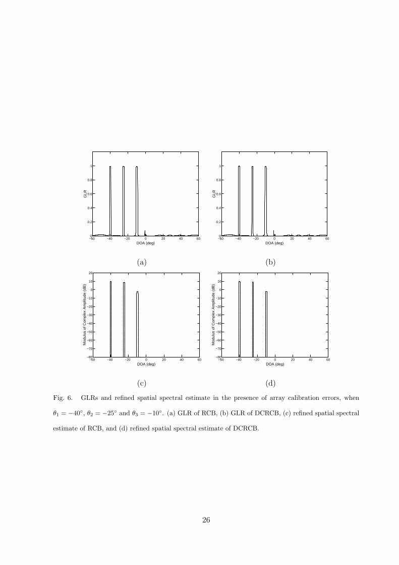
Figs. 6(a)-6(b) show the GLRs corresponding to RCB and DCRCB, as functions of θ,
which are obtained by replacing ar(θ) in (34) by ar(θ) and ˆar(θ) from Subsections IV-A
15
and IV-B, respectively. As we can see, both RCB and DCRCB give high GLRs at the
target locations and a low GLR at the jammer location. Based on the GLRs, we can again
readily and correctly estimate the number of targets to be 3. Plotting the spatial spectral
estimates in Figs. 5(c) and 5(d) only for the angles at which the corresponding GLRs are
above a given threshold (say 0.8), we obtain the refined spatial spectral estimates in Figs.
6(c) and 6(d). These refined spatial spectral estimates obtained by RCB and DCRCB
provide an accurate description of the target scenario.
VI. Conclusions
We have considered several adaptive techniques for a MIMO radar system, where mul-
tiple antennas transmit linearly independent (perferrably uncorrelated) waveforms and
multiple antennas receive the reflected signals. Due to the different phase shifts caused
by the different propagation paths from the transmitting antennas to the targets, these
linearly independent waveforms are combined with different phase factors at the targets.
The result is that the signals reflected from different targets are linearly independent of
each other, which enables the application of the adaptive techniques to achieve high reso-
lution and superior interference and jamming rejection capability. In the absence of array
calibration errors, we have considered Capon, APES and CAPES. Capon provides high
resolution and APES gives accurate amplitude estimates at the target locations, while
CAPES combines the merits of both Capon and APES. We have also introduced a new
approach, referred to as CAML, which can further improve the amplitude estimation ac-
curacy of (C)APES. In the presence of array calibration errors, we have shown that the
RCB and DCRCB approaches can provide accurate estimates of both target locations and
16
target amplitudes. Finally, we have proposed a generalized likelihood ratio test that can
be used to determine the number of targets by separating the jammers from targets.
Appendix: Generalized Likelihood Ratio Test
We assume that the columns of the residual term Z in (1) are independently and identi-
cally distributed circularly symmetric complex Gaussian random vectors with zero-mean
and unknown covariance matrix Q. We derive the GLRT for each θ of interest. For
notational brevity, we omit the argument θ of ρ, ar, at and β.
Following [25] (see also [26]), we define the GLR as follows:
ρ = 1−[maxQ f(X|β = 0,Q)
maxβ,Q f(X|β,Q)
] 1L
, (35)
where
f(X|β,Q) = π−LM |Q|−L exp{−tr
[Q−1(X− arβaT
t S)(X− arβaTt S)H
]}(36)
is the probability density function of the observed data matrix X given the parameters
β and Q, and tr(·) and | · | denote the trace and determinant of a matrix, respectively.
From (35), we note that the value of the GLR, ρ, lies between 0 and 1. If there is a target
at a θ of interest, we usually have maxβ,Q f(X|β,Q) À maxQ f(X|β = 0,Q), i.e., ρ ≈ 1;
otherwise ρ ≈ 0.
Solving the optimization problems in (35) with respect to Q yields
maxQ
f(X|β = 0,Q) = (πe)−LM |R|−L, (37)
and
maxβ,Q
f(X|β,Q) = (πe)−LM
{min
β
∣∣∣∣1
L(X− arβaT
t S)(X− arβaTt S)H
∣∣∣∣}−L
. (38)
17
Applying the technique used in [10] and [27], we obtain
∣∣∣∣1
L(X− arβaT
t S)(X− arβaTt S)H
∣∣∣∣
=
∣∣∣∣R− XSHa∗t β∗aH
r
L− arβaT
t SXH
L+ |β|2ara
Tt RSSa
∗ta
Hr
∣∣∣∣
=
∣∣∣∣∣∣Q + (aT
t RSSa∗t )
(arβ − XSHa∗t
L(aTt RSSa∗t )
)(arβ − XSHa∗t
L(aTt RSSa∗t )
)H∣∣∣∣∣∣
=|Q|∣∣∣∣∣∣I + (aT
t RSSa∗t ) Q
−1
(arβ − XSHa∗t
L(aTt RSSa∗t )
)(arβ − XSHa∗t
L(aTt RSSa∗t )
)H∣∣∣∣∣∣
=|Q|1 + (aT
t RSSa∗t )
(arβ − XSHa∗t
L(aTt RSSa∗t )
)H
Q−1
(arβ − XSHa∗t
L(aTt RSSa∗t )
)
≥|Q|[1 +
aTt SXH
L2(aTt RSSa∗t )
Q−1
(I− ara
Hr Q−1
aHr Q−1ar
)XSHa∗t
],
(39)
where we have used the fact that |I + AB| = |I + BA| [16], and the equality holds when
β = βAPES. Note that
|Q|[1 +
aTt SXH
L2(aTt RSSa∗t )
Q−1
(I− ara
Hr Q−1
aHr Q−1ar
)XSHa∗t
]
=|Q|∣∣∣∣∣I + Q−1
(I− ara
Hr Q−1
aHr Q−1ar
)XSHa∗ta
Tt SXH
L2(aTt RSSa∗t )
∣∣∣∣∣
=
∣∣∣∣∣Q +
(I− ara
Hr Q−1
aHr Q−1ar
)XSHa∗ta
Tt SXH
L2(aTt RSSa∗t )
∣∣∣∣∣
=
∣∣∣∣∣R− araHr Q−1XSHa∗ta
Tt SXH
L2(aHr Q−1ar)(aT
t RSSa∗t )
∣∣∣∣∣
=|R|∣∣∣∣∣I−
R−1araHr Q−1XSHa∗ta
Tt SXH
L2(aHr Q−1ar)(aT
t RSSa∗t )
∣∣∣∣∣
=|R|[1− aH
r Q−1(R− Q)R−1ar
aHr Q−1ar
]
=|R| aHr R−1ar
aHr Q−1ar
,
(40)
where again we have used the fact that |I + AB| = |I + BA|.
18
From (39) and (40), it follows that
minβ
∣∣∣∣1
L(X− arβaT
t S)(X− arβaTt S)H
∣∣∣∣ = |R| aHr R−1ar
aHr Q−1ar
. (41)
By using (37), (38), and (41) in (35), the GLR in (34) follows immediately.
References
[1] D. W. Bliss and K. W. Forsythe, “Multiple-input multiple-output (MIMO) radar and imaging: degrees of
freedom and resolution,” Proceedings of the 37th Asilomar Conference on Signals, Systems and Computers,
vol. 1, pp. 54–59, Nov. 2003.
[2] E. Fishler, A. Haimovich, R. Blum, D. Chizhik, L. Cimini, and R. Valenzuela, “MIMO radar: an idea whose
time has come,” Proceedings of the IEEE Radar Conference, pp. 71–78, April 2004.
[3] E. Fishler, A. Haimovich, R. Blum, L. Cimini, D. Chizhik, and R. Valenzuela, “Performance of MIMO radar
systems: advantages of angular diversity,” Proceedings of the 38th Asilomar Conference on Signals, Systems
and Computers, vol. 1, pp. 305–309, Nov. 2004.
[4] E. Fishler, A. Haimovich, R. Blum, L. Cimini, D. Chizhik, and R. Valenzuela, “Spatial diversity in radars -
models and detection performance,” IEEE Transactions on Signal Processing, to appear.
[5] D. R. Fuhrmann and G. S. Antonio, “Transmit beamforming for MIMO radar systems using partial signal
correlation,” Proceedings of the 38th Asilomar Conference on Signals, Systems and Computers, vol. 1, pp. 295–
299, Nov. 2004.
[6] F. C. Robey, S. Coutts, D. D. Weikle, J. C. McHarg, and K. Cuomo, “MIMO radar theory and exprimental
results,” Proceedings of the 38th Asilomar Conference on Signals, Systems and Computers, vol. 1, pp. 300–304,
Nov. 2004.
[7] K. W. Forsythe, D. W. Bliss, and G. S. Fawcett, “Multiple-input multiple-output (MIMO) radar: performance
issues,” Proceedings of the 38th Asilomar Conference on Signals, Systems and Computers, vol. 1, pp. 310–314,
Nov. 2004.
[8] L. B. White and P. S. Ray, “Signal design for MIMO diversity systems,” Proceedings of the 38th Asilomar
Conference on Signals, Systems and Computers, vol. 1, pp. 973 – 977, Nov. 2004.
[9] J. Capon, “High resolution frequency-wavenumber spectrum analysis,” Proceedings of the IEEE, vol. 57,
pp. 1408–1418, August 1969.
[10] J. Li and P. Stoica, “An adaptive filtering approach to spectral estimation and SAR imaging,” IEEE Trans-
actions on Signal Processing, vol. 44, pp. 1469–1484, June 1996.
19
[11] A. Jakobsson and P. Stoica, “Combining Capon and APES for estimation of spectral lines,” Circuits, Systems
and Signal Processing, vol. 19, pp. 159–169, 2000.
[12] L. Xu, P. Stoica, and J. Li, “A diagonal growth curve model and some signal processing ap-
plications,” to appear in IEEE Transactions on Signal Processing, (Available on the website:
ftp://www.sal.ufl.edu/xuluzhou/DGC.pdf).
[13] J. Li, P. Stoica, and Z. Wang, “On robust Capon beamforming and diagonal loading,” IEEE Transactions on
Signal Processing, vol. 46, pp. 1954–1966, July 2003.
[14] P. Stoica, Z. Wang, and J. Li, “Robust Capon beamforming,” IEEE Signal Processing Letters, vol. 10,
pp. 172–175, 2003.
[15] J. Li, P. Stoica, and Z. Wang, “Doubly constrained robust Capon beamformer,” IEEE Transactions on Signal
Processing, vol. 52, pp. 2407–2423, September 2004.
[16] P. Stoica and R. Moses, Spectral Analysis of Signals. NJ: Prentice-Hall, 2005.
[17] P. Stoica, H. Li, and J. Li, “A new derivation of the APES filter,” IEEE Signal Processing Letters, vol. 6,
pp. 205–206, August 1999.
[18] E. Larsson, J. Li, and P. Stoica, “High-resolution nonparametric spectral analysis: Theory and applications.
in high-resolution and robust signal processing (Y. Hua, A. Gershman and Q. Cheng, eds.),” pp. 151–251,
2004.
[19] P. Stoica, A. Jakobsson, and J. Li, “Capon, APES and matched-filterbank spectral estimation,” Signal Pro-
cessing, vol. 66, pp. 45–59, April 1998.
[20] H. Li, J. Li, and P. Stoica, “Performance analysis of forward-backward matched-filterbank spectral estima-
tors,” IEEE Transactions on Signal Processing, vol. 46, pp. 1954–1966, July 1998.
[21] D. A. Harville, Matrix Algebra from a Statistician’s Perspective. New York, NY: Springer, Inc., 1997.
[22] K. M. Buckley and L. J. Griffiths, “An adaptive generalized sidelobe canceller with derivative constraints,”
IEEE Transactions on Antennas and Propagation, vol. 34, pp. 311–319, March 1986.
[23] T. L. Marzetta, “A new interpretation for Capon’s maximum likelihood method of frequency-wavenumber
spectrum estimation,” IEEE Transactions on Acoustics, Speech, and Signal Processing, vol. 31, pp. 445–449,
April 1983.
[24] P. Stoica and G. Ganesan, “Maximum-SNR spatial-temporal formatting designs for MIMO channels,” IEEE
Transactions on Signal Processing, vol. 50, pp. 3036–3042, December 2002.
[25] E. J. Kelly, “An adaptive detection algorithm,” IEEE Transactions on Aerospace and Electronics Systems,
vol. 22, pp. 115–127, March 1986.
[26] A. Dogandzic and A. Nehorai, “Generalized multivariate analysis of variance,” IEEE Signal Processing Mag-
20
azine, pp. 39–54, September 2003.
[27] Y. Jiang, P. Stoica, and J. Li, “Array signal processing in the known waveform and steering vector case,”
IEEE Transactions on Signal Processing, vol. 52, pp. 23–35, January 2004.
21
s 1
s 2
s N
x 1 x
2 x
M ... ...
...
Targets
Transmitting array Receiving array
Fig. 1. A MIMO radar system.
22
−60 −40 −20 0 20 40 600
0.5
1
1.5
2
2.5
3
3.5
4
4.5
5
DOA (deg)
Mod
ulus
of C
ompl
ex A
mpl
itude
−60 −40 −20 0 20 40 600
0.5
1
1.5
2
2.5
3
3.5
4
4.5
5
DOA (deg)
Mod
ulus
of C
ompl
ex A
mpl
itude
(a) (b)
−60 −40 −20 0 20 40 600
0.5
1
1.5
2
2.5
3
3.5
4
4.5
5
DOA (deg)
Mod
ulus
of C
ompl
ex A
mpl
itude
−60 −40 −20 0 20 40 600
0.2
0.4
0.6
0.8
1
DOA (deg)
GLR
(c) (d)
−60 −40 −20 0 20 40 600
0.5
1
1.5
2
2.5
3
3.5
4
4.5
5
DOA (deg)
Mod
ulus
of C
ompl
ex A
mpl
itude
−60 −40 −20 0 20 40 600
0.5
1
1.5
2
2.5
3
3.5
4
4.5
5
DOA (deg)
Mod
ulus
of C
ompl
ex A
mpl
itude
(e) (f)
Fig. 2. Spatial spectral estimates and GLR in the absence of array calibration errors, when θ1 = −40◦,
θ2 = −25◦ and θ3 = −10◦. (a) LS, (b) Capon, (c) APES, (d) GLR, (e) CAPES, and (f) CAML.
23
−60 −40 −20 0 20 40 600
0.5
1
1.5
2
2.5
3
3.5
4
4.5
5
DOA (deg)
Mod
ulus
of C
ompl
ex A
mpl
itude
−60 −40 −20 0 20 40 600
0.5
1
1.5
2
2.5
3
3.5
4
4.5
5
DOA (deg)
Mod
ulus
of C
ompl
ex A
mpl
itude
(a) (b)
−60 −40 −20 0 20 40 600
0.5
1
1.5
2
2.5
3
3.5
4
4.5
5
DOA (deg)
Mod
ulus
of C
ompl
ex A
mpl
itude
−60 −40 −20 0 20 40 600
0.2
0.4
0.6
0.8
1
DOA (deg)
GLR
(c) (d)
−60 −40 −20 0 20 40 600
0.5
1
1.5
2
2.5
3
3.5
4
4.5
5
DOA (deg)
Mod
ulus
of C
ompl
ex A
mpl
itude
−60 −40 −20 0 20 40 600
0.5
1
1.5
2
2.5
3
3.5
4
4.5
5
DOA (deg)
Mod
ulus
of C
ompl
ex A
mpl
itude
(e) (f)
Fig. 3. Spatial spectral estimates and GLR in the absence of array calibration errors, when θ1 = −40◦,
θ2 = −25◦ and θ3 = −21◦. (a) LS, (b) Capon, (c) APES, (d) GLR, (e) CAPES, and (f) CAML.
24
−40 −30 −20 −10 0 10 20 30−0.8
−0.7
−0.6
−0.5
−0.4
−0.3
−0.2
−0.1
0
0.1
SNR (dB)
Bia
s CaponCAPESCAML
−40 −30 −20 −10 0 10 20 3010
−10
10−8
10−6
10−4
10−2
100
102
SNR (dB)
MS
E
CaponCAPESCAML
(a) (b)
Fig. 4. Empirical Bias and MSE versus SNR in the absence of array calibration errors, when θ1 = −40◦,
θ2 = −25◦, and θ3 = −21◦. (a) Bias and (b) MSE.
−60 −40 −20 0 20 40 60−80
−70
−60
−50
−40
−30
−20
−10
0
10
20
DOA (deg)
Mod
ulus
of C
ompl
ex A
mpl
itude
(dB
)
−60 −40 −20 0 20 40 60−80
−70
−60
−50
−40
−30
−20
−10
0
10
20
DOA (deg)
Mod
ulus
of C
ompl
ex A
mpl
itude
(dB
)
(a) (b)
−60 −40 −20 0 20 40 60−80
−70
−60
−50
−40
−30
−20
−10
0
10
20
DOA (deg)
Mod
ulus
of C
ompl
ex A
mpl
itude
(dB
)
−60 −40 −20 0 20 40 60−80
−70
−60
−50
−40
−30
−20
−10
0
10
20
DOA (deg)
Mod
ulus
of C
ompl
ex A
mpl
itude
(dB
)
(c) (d)
Fig. 5. Spatial spectral estimates in the presence of array calibration errors, when θ1 = −40◦, θ2 = −25◦
and θ3 = −10◦. (a) Capon, (b) APES, (c) RCB with ε = 0.1 , and (d) DCRCB with ε = 0.1.
25
−60 −40 −20 0 20 40 600
0.2
0.4
0.6
0.8
1
DOA (deg)
GLR
−60 −40 −20 0 20 40 600
0.2
0.4
0.6
0.8
1
DOA (deg)
GLR
(a) (b)
−60 −40 −20 0 20 40 60−80
−70
−60
−50
−40
−30
−20
−10
0
10
20
DOA (deg)
Mod
ulus
of C
ompl
ex A
mpl
itude
(dB
)
−60 −40 −20 0 20 40 60−80
−70
−60
−50
−40
−30
−20
−10
0
10
20
DOA (deg)
Mod
ulus
of C
ompl
ex A
mpl
itude
(dB
)
(c) (d)
Fig. 6. GLRs and refined spatial spectral estimate in the presence of array calibration errors, when
θ1 = −40◦, θ2 = −25◦ and θ3 = −10◦. (a) GLR of RCB, (b) GLR of DCRCB, (c) refined spatial spectral
estimate of RCB, and (d) refined spatial spectral estimate of DCRCB.
26
Top Related