


Languages
Pages
Legal


A Virtualised Routing Protocol for Improving
Network Lifetime in Cluster Based Sensor
Networks
Ruslan Saad Abdulrahman Al-Nuaimi
College of Science and Technology
School of Computing, Science and Engineering
University of Salford, Manchester, UK
Submitted in Partial Fulfilment of the Requirements of the
Degree of Doctor of Philosophy
2017

i
Table of Contents
Table of Contents ………………………………………………………………….. i
List of Figures …………………………………………………………………….. viii
List of Tables ……………………………………………………………………… xii
List of Pseudo Codes ………………………………………………………………. xiii
Acknowledgements ……………………………………………………………….. xiv
List of Abbreviations ………………………………………………………………. xv
Abstract ……………………………………………………………………………. 1
Chapter One: Introduction 2
1-1 Introduction …………………………………………………………………… 2
1-2 Network Function Virtualisation (NFV) ……………………………………… 4
1-3 Research Problem ……………………………………………………………... 5
1-4 Research Question…………………………………………………………….. 8
1-5 Research Aims and Objectives ………………………………………………… 8
1-6 Contribution of the thesis ……………………………………………………… 9
1-7 Research Process ………………………………………………………………. 10
1-8 Thesis Layout ………………………………………………………………….. 14
Chapter Two: An Overview of Wireless Sensor Networks 16
2-1 Wireless Sensor Networks Background ……………………………………… 16
2-2 Wireless Sensor Networks Characteristics …………………………………….. 18
2-3 Sensor Nodes Architecture …………………………………………………….. 21
2-4 Wireless Sensor Network Applications ……………………………………….. 22
2-5 Wireless Sensor Network Protocol Stack ……………………………………… 24

ii
2-6 Routing Protocols in WSN …………………………………………………… 26
2-6-1 Design Requirements for WSN Routing Protocols ……………………. 28
2-6-2 Classification of Routing Protocols in WSN …………………………… 30
2-6-2-1 Network structure-Based Routing Protocols …………………… 31
I. Flat Routing Protocols Routing Protocols …………………………… 31
II. Hierarchical Routing Protocols Routing Protocols ………………….. 31
III. Location-Based Protocols Routing Protocols ……………………….. 31
2-6-2-2 Protocol Operation-Based Routing Protocols ……………………. 32
I. Query-Based Routing Protocols …………………………………….. 32
II. Multipath-Based Routing Protocols ………………………………… 32
III. Negotiation-Based Routing Protocols ………………………………. 32
IV. QoS Based Routing Protocols ….…………………………………….. 33
V. Non-Coherent and Coherent Based Routing Protocols ….…………… 33
2-6-2-3 Routes Establishment ……..……………………………………..... 33
I. Proactive Routing Protocols …………………………………………. 34
II. Reactive Routing Protocols ………………………………………….. 34
III. Hybrid Routing Protocols ……………………………………………. 34
2-7 Energy Consumption in Wireless Sensor Networks …………………………... 35
2-7-1 Sensor Node and Network Lifetime …………………………................. 40
2-8 Summery ……………………………………………………………………… 41
Chapter Three: Literature Review of Clustering based Routing
Protocols in Wireless Sensor Network 42
3-1 Introduction ……………………………………………………………………. 42

iii
3-2 The Clustering Approach ……………………………………………………… 42
3-4 Clustering Based Routing Protocols ……………………………………..….… 50
3-4-1 Distributed Clustering Protocols ……………………………………….. 51
1- LEACH Low-Energy Adaptive Clustering Hierarchy (LEACH) …… 52
2- LEACH-Balanced (LEACH-B)……………………………………… 56
3- Extended-LEACH (E-LEACH) ………………………………………. 57
4- Energy-Efficient LEACH (EE-LEACH) …………………………….. 57
5- Energy Efficient Extended LEACH (EEE LEACH) ………………… 57
6- Power-Efficient Gathering Sensor Information Systems (PEGASIS) ... 58
7- PEGASIS-LEACH …………………………………………………….. 58
8- Threshold sensitive Energy Efficient Sensor Network Protocol (TEEN). 58
9- Adaptive Periodic-TEEN (APTEEN) ……………………………….. 59
10- LEACH-Selective Cluster (LEACH-SC)……………………………. 59
11- Narrative-LEACH …………………………………………………… 59
12- Two Level (TL-LEACH) …………………………………………… 60
13- Double Cluster Based Energy Efficient Routing Protocol ………….. 60
14- Cognitive LEACH ………………………………………………….. 61
15- Solar LEACH (SLEACH) ………………………………………….. 61
16- Hybrid Energy-Efficient Distributed Clustering Protocol (HEED)….. 61
17- Unequal Cluster-based Routing protocol (UCR) …………………….. 62
18- Centralised Energy Efficient Distance Protocol (CEED) …………... 62
19- Unequal Clustering Routing for Mobile Education Protocol ……….. 63
20- Double-phase Cluster-head Election Clustering Protocol (DEC) …… 63
21- Energy potential-LEACH (EP-LEACH) ………..………..………….. 63

iv
3-4-2 Centralised Clustering Protocol ……………………………………....... 64
1- Centralized LEACH (LEACH-C) ……………………………………. 65
2- Modified LEACH-C ………………………………………………… 67
3- LEACH Central Constrained (LEACH-CC) ………………………… 67
4- Energy Efficient LEACH-C (EELEACH-C) ………………………… 67
5- Base-Station Controlled Dynamic Clustering Protocol (BCDCP) …… 68
6- Centralised Genetic-Based Clustering (CGC) ……………………….. 68
7- Centralized Balance Clustering Routing Protocol …………………….. 68
3-5 Critical Analysis ………………………………………………………………. 76
3-6 Summary ………………………………………………………………………. 76
Chapter Four: A Virtualised Clustering Routing Protocol (VCR) 78
4-1 Introduction ……………………………………………………………………. 78
4-2 The Assumptions of the VCR …………………………………........................ 78
4-3 VCR Protocol Functions ….………………………………………………….. 81
4-3-1 Node Discovery Function ……………………………………………….. 84
4-3-2 Information calculation Function ………………………………………... 86
4-3-3 Clustering Function ……………………………………………………… 90
4-3-3-1 Setup Stage (cluster formation and cluster head selection by NFV
server) ………………………………………………………………….. 90
Step 1- Calculate Optimum Number Of Clusters ………………. 90
Step 2- Cluster Formation ……………………………………….. 92
Step 3- Cluster Head Selection ………………………………… 97
4-3-3-2 Setup Stage (prepare the necessary data for transmission to the
nodes).......................................................................................... 98

v
4-3-3-3 Steady state stage (data transmission) ……………………..…… 99
4-3-4 Schedule Formation …………………………………..……………………… 101
4-4 Energy Consumption Calculation Function ………………………………….. 102
4-5 Cluster Head re-selection Function ……………………………………………. 103
4-6 Re-Clustering Function ………………………………………………………. 105
4-7 Summary ……………………………………………………………………… 106
Chapter Five: The Developed Mathematical model for Virtualised
Clustering Routing Protocol (VCR) 108
5-1 Introduction …………………………………………………………………… 108
5-2 Radio Energy Model ………………………………………………………….. 108
5-3 Analysis of the Energy Consumption of the VCR……..…………………….. 110
5-3-1 Energy Consumption Model in Node Discovery (Broadcasting) ……… 112
5-3-2 Cluster Head (CH) node energy consumption per cycle ……………….. 113
5-3-3 Non-Cluster Head (CH) energy consumption per cycle ……………….. 114
5-3-4 Remaining energy level for CHs and Cluster members’ nodes ………… 116
5-3-5 Total network energy consumption per cycle ……………………………. 117
5-3-6 Total network energy consumption per cycle ……………………………. 117
5-4 Analysis of power consumption in the LEACH protocol …………………… 117
5-4-1 Energy Consumption Model in Processing ……………………………… 118
5-4-2 Energy Consumption Model for Cluster Head Node ……………………. 119
5-4-3 Energy Consumption Model for Cluster Member Node ………………… 121
5-5 Summary ………………………………………………………………………. 123
Chapter Six : Simulation, Validation Results and Evaluation 125
6-1 Introduction ……………………………………………………………………. 125

vi
6-2 Experimental Design …………………………………….…………………….. 125
6-2-1 Validation Experiments …………………….…………………………… 125
6-2-2 Evaluation Experiments ……………………….………………………… 126
6-3 Network Topology Setup ……………………………………………………… 127
6-4 Calculation of the Optimum Number of Clusters …………………………….. 129
6-5 Clusters Formation …………………………………………………………….. 130
6-6 Results and Validation ………………………………………………………. 131
6-6-1 Energy Consumption Calculation ………………………………………. 131
1- Experiment One: number of nodes 100, sink location 50,175 and
sensing area size (100*100) ………………………………………….. 132
2- Experiment Two (change Sink Position and area size) ……………… 133
3- Experiment Three (based on different number of clusters) ………… 135
3-1 Scenario One: When Number of Nodes=50 …………………… 135
3-2 Scenario Two: When Number of Nodes=150 ………………….. 136
3-3 Scenario Three: When Number of Nodes=200 ………………… 137
4- Experiment Four: Various node density within the clusters (Different
number of Nodes) ………………………………………………… 138
5- Experiment Five: Scenario 5: Dynamic and Static clustering in VCR 139
6-7 Evaluation ……………………………………………………………………. 140
6-7-1 Experiment Six: Lifetime measurement based on First Node Dead (FND) 141
6-7-2 Experiment Seven: Start-up Cost ….…………………………………… 142
6-7-3 Experiment Eight: Round Rotation ……………………………………… 144
6-8 Results Analysis ……………………………………………………………….. 145
6-9 Summary ………………………………………………………………………. 146
Chapter Seven: Conclusions and Future works 149

vii
7-1 Introduction ……………………………………………………………………. 149
7-2 Conclusions ……………………………………………………………………. 149
7-3 Future Works ………………………………………………………………… 152
Publications ………………………………………………………………………… 154
References …………………………………………………………………………. 155
Appendix A: PDUs …………. …………………………………………………… 169
Appendix B: Protocol Diagram ……………………………………………………. 177
Appendix C: Virtualised Clustering Routing (VCR) Protocol Flow Chart………… 178
Appendix D: Network Topologies ………………………………………………… 179
Appendix E (K-means convergence iterations for different topologies, nodes density
and number of clusters) …......................................................................................... 182

viii
List of Figures
Figure (1-1) NFV Vision …………………………………………………………….. 5
Figure (1-2) Research Process ……………………………………………………… 10
Figure (2-1) Simple Diagram of a WSN …………………………………………….. 17
Figure (2-2) Sensor Node’s Architecture ……………………………………………. 22
Figure (2-3) WSN Applications ……………………………………………………... 24
Figure (2-4) WSN Protocol Stack …………………………………………………… 25
Figure (2-5) WSN Communications type …………………………………………… 27
Figure (2-6) Routing Protocols Classifications ……………………………………… 30
Figure (2-7) Energy Consumption Domains ………………………………………… 37
Figure (2-8) Sensing Component Modes …………………………………………… 38
Figure (2-9) Transceiver Component Mode ………………………………………… 38
Figure (2-10) Processing Component Mode ………………………………………… 38
Figure (3-1) Architecture of cluster-based routing protocols ……………………….. 43
Figure (3-2) Clustering Function Stages …………………………………………….. 44
Figure (3-3) Clustering Proprieties ………………………………………………….. 44
Figure (3-4) Clustering Model ………………………………………………………. 47
Figure (3-5) Clustering Timing …………………………………………………….. 48
Figure (3-6) Clustering Routing Protocols classification …………………………… 50
Figure (3-7) Distributed Clustering Protocol Flowchart……………………………… 51
Figure (3-8) LEACH round timeline ……………………………………………….. 53
Figure (3-9) LEACH operation flow chart …………………………………………. 55

ix
Figure (3-10) LEACH communications fields ………………………………………. 55
Figure (3-11) Centralised Clustering Protocol Flowchart …………………………… 65
Figure (3-12) LEACH-C operation flow chart ………………………………………. 66
Figure (3-13) Proposed Protocol (VCR) operation flow chart ………………………. 77
Figure (4-1) Virtual Clustering Routing Protocol Characteristics ………………….. 80
Figure (4-2) VCR Clustering cycle ………………………………………………….. 82
Figure (4-3) VCR diagram.…………………………………………………………. 83
Figure (4-4) VCR Communications Fields …………………………………………. 84
Figure (4-5) Node Discovery Function ………….……………………………… …. 85
Figure (4-6) Node Discovery Packet (SN_Dis_PDU) ……………………………… 85
Figure (4-7) Sink_Server_Discovery Packet (Sink_Server_Dis_PDU) ……………. 85
Figure (4-8) Information Calculations Function ……………………………………. 86
Figure (4-9) Clustering Function ……………………………………………………. 90
Figure (4-10) K-means algorithm ……………………………………………………. 95
Figure (4-11) Cluster Formation Diagram ………………………………………….. 96
Figure (4-12) Server to Sink Cluster Information Packet (Cl_Inf_Server_sink_PDU) 98
Figure (4-13) Sink to Node Cluster Information Packet (Cl_Inf_Sink_Node_PDU) 99
Figure (4-14) Sensed Data Info (Sense_Data_Info) ………………………………… 99
Figure (4-15) Aggregated Data Info (Agg_Data_Info) …………………………... 100
Figure (4-16) Steady state stage …………………………………………………….. 100
Figure (4-17) Notification Packet (Notification_PDU) …………………………….. 101
Figure (4-18) Cluster Head re-selection Function…………………………………… 104
Figure (4-19) Cluster Head re-selection Packet (Reslect_CH_Packet) ……………… 104
Figure (4-20) Cluster Head re-selection Packet (Reslect_CH_Sink_Node_Packet) .. 105

x
Figure (4-21) Re-Clustering Function ……………………………………………… 106
Figure (5-1) Radio Energy Consumption Model (redraw from [1]) ………………… 108
Figure (5-2) Energy Consumption Chart for VCR ………………………………… 111
Figures (6-1) Network Topology Example …………………………………………. 128
Figures (6-2) K-means average convergence iterations …………………………….. 130
Figure (6-3) Average Energy Consumption with N=100 …………………………… 132
Figure (6-4) Average Energy Consumption with varying sink position…………….. 134
Figure (6-5) Average Energy Consumption with different sensing area size……….. 135
Figure (6-6) Optimum Number of Clusters for N=50 ……………………………….. 136
Figure (6-7) Optimum Number of Clusters for N=150 ……………………………… 137
Figure (6-8) Optimum Number of Clusters for N=200 ……………………………… 137
Figure (6-9) Average Energy Consumption with different nodes density ………….. 138
Figure (6-10) Static vs Dynamic Clustering in VCR ……………………………….. 140
Figure (6-11) Comparison among VCR, LEACH and LEACH-C…………………. 142
Figure (6-12) Start-Up Energy Consumption ……………………………………….. 143
Figure (6-13) Static Proposed Protocol vs. Static LEACH ………………………….. 145
Figure (A-1) Type of Packet (ToP) …….………………………………………….. 169
Figure (A-2) General Packet Format ……………………………………………….. 169
Figure (A-3) Node Discovery Packet (SN_Dis_PDU) ………………………........... 170
Figure (A-4) Sink_Server_Discovery Packet (Sink_Server_Dis_PDU) …………… 170
Figure (A-5) Server to Sink Cluster Information Packet (Cl_Inf_Server_sink_PDU).. 171
Figure (A-6) Sink to Node Cluster Information Packet (Cl_Inf_Sink_Node_PDU) … 172
Figure (A-7) Sensed Data Info (Sense_Data_Info) …………………………………. 173
xi
Figure (A-8) Aggregated Data Packet (Agg_Data_PDU) …………………………… 174
Figure (A-9) End Cycle Notification Packet (End_Cycle_notify_PDU) ……………. 174
Figure (A-10) Cluster Head re-selection Packet (Reslect_CH_Server_Sink_Packet).. 175
Figure (A-11) Cluster Head re-selection Packet (Reslect_CH_Sink_Node_Packet)… 175
Figure (C-1) Virtualised Clustering Routing (VCR) Protocol Flow Chart …………. 178
Figures (D-1) Network Topologies with various seed values ……………………….. 181
Figures (E-1) K-means coverage with two clusters …………………………………. 182
Figures (E-2) K-means coverage with three clusters ……………………………….. 182
Figures (E-3) K-means coverage with four clusters ………………………………… 182
Figures (E-4) K-means coverage with five clusters …………………………………. 183
Figures (E-5) K-means coverage with six clusters ………………………………….. 183
Figures (E-6) K-means coverage with seven clusters ……………………………….. 183
Figures (E-7) K-means coverage with eight clusters ……………………………….. 184
Figures (E-8) K-means coverage with nine clusters ………………………………… 184
Figures (E-9) K-means coverage with ten clusters ………………………………….. 184

xii
List of Tables
Table (3-1) Comparison among Clustering based Routing Protocols in WSN. 70
Table (5-1) Number of Communications for proposed protocol and LEACH.. 123
Table (6-1) Simulation Parameters ………………………………………… 128
Table (6-2) Range of Clusters ……………………………………………… 129
Table (6-3) Comparison among LEACH, LEACH-C and VCR …………… 147

xiii
List of Pseudo Codes
Code (4-1) Pseudo Code for Distance between Sensor Nodes and the Sink 88
Code (4-2) Distance between sensor nodes pseudo code 89
Code (4-3) Pseudo Code for Cost Function Calculation 89
Code (4-4) Cluster head selection code 97
Code (6-1) Pseudo Codes for Sensor Node and Sink Deployment 127

xiv
ACKNOWLEDGEMENTS
Firstly, I would like to extend my thanks and appreciation to my supervisor Dr.Adil Al-
Yasiri for his support, encouragement, motivation, enthusiasm, and immense knowledge during
the research period. Your advice on research has been invaluable.
My thankful go to the Iraqi Ministry of Higher Education and Scientific Research who
was the funding of my PhD study. My thanks also go out to the support that I received from the
Iraqi Cultural Attaché-London who were always so helpful. In addition, I would like to thank
my university in Iraq (Al-Nahrain University) to nominated me for this scholarship.
I would like to extend my thanks and gratitude to my husband “Aws” for his support,
encouragement and patience throughout stages of this PhD. Thank you. I dedicate this thesis to
you.
In addition, I would like to say a heartfelt thank you to my Dad, Mom, sisters and brother
for always believing in me and encouraging me to follow my dreams and helping in whatever
way they could during this challenging period.
Last but not least, I thank the school of Computer Science and Engineering, the
University of Salford for providing the support and favorable environment during the research
period.
xv
List of Abbreviations
APTEEN Adaptive Periodic TEEN
BCDCP Base-Station Controlled Dynamic Clustering Protocol
CEED Centralised Energy Efficient Distance
CGC Centralised Genetic-Based Clustering
CH Cluster Head
CM Cluster Member
CN Centroid Node
DEC Double-phase Cluster-head Election Clustering Protocol
DL-LEACH Double Cluster Based Energy Efficient Routing Protocol
EAGR Energy Aware Greedy Routing
EEE-LEACH Energy Efficient Extended LEACH
EE-LEACH Energy-Efficient LEACH
EE-LEACH-C Energy Efficient LEACH-C
E-LEACH Extended LEACH
EP-LEACH Energy potential LEACH
ETSI European Telecommunications Standards Institute
FND First Dead Node
GAF Geographic Adaptive Fidelity
GEAR Geographical and Energy-Aware Routing Protocol
GPS Geographical Position System
HEED Hybrid Energy-Efficient Distributed clustering
HND Half Nodes Die
ID Identification
IP Internet Protocol

xvi
LEACH Low-Energy Adaptive Clustering Hierarchy
LEACH-B LEACH-Balanced
LEACH-C Centralized LEACH
LEACH-CC LEACH Central Constrained
LEACH-F Fixed- LEACH
LEACH-SC LEACH-Selective Cluster
LND Last Nodes Die
MAC Media Access Control
MANET Mobile ad hoc Network
MATLAB Matrix Laboratory
MEMS Micro-Electro-Mechanical Systems
MWE Multiple Winner Algorithm
N- LEACH Narrative-LEACH
NFV Network Function Virtualisation
PDU Protocol Data Unit
PEGASIS Power-Efficient Gathering in Sensor Information Systems
QoS Quality of Service
SAR Sequential Assignment Routing
S-LEACH Solar LEACH
SN Sensor Node
SPEED Stateless Protocol for Real-Time Communication in Sensor Networks
SPIN Sensor Protocol for Information via Negotiation
SWE Single Winner Algorithm
ToP Type Of Packet
VCR Virtualised Clustering Routing
1
Abstract
In Wireless Sensor Networks (WSN), enhancing network lifetime is one of the critical
challenges that should be considered during the network design. Sensor nodes exhaust their
power in various activities such as sensing, processing and communication that represents the
most energy-consuming and therefore should be managed to improve the network lifetime.
The clustering has a significant task on network lifetime because sensor nodes consume
a considerable amount of energy during the transmission and receiving in order to perform the
clustering function stages. Clustering is the process of grouping sensor nodes into groups that
are administered by a node known as a cluster head (CH). The main stages of this function are
the setup stage, responsible for the cluster formation and cluster head selection, and the steady
state stage (data transmission). By managing and reducing the number and amounts of
communications as well as computation during these stages efficiently, will affect the nodes’
energy consumption and enhance network lifetime.
The aim of this thesis is to improve the network lifetime by virtualising the clustering
function to be implemented into high-volume central server on the cloud as well as using
efficient approaches in cluster formation (based on k-means algorithm) and in cluster head
selection (based on current nodes energy level and their distance to sink). These processes will
result in a reduction in the number and amount of communication messages and the
computational needs for each node during clusters formation and cluster head selection, thus
improving the network’s lifetime. Hence, a new virtualised clustering routing protocol based
on Network Function Virtualisation (NFV) has been proposed. NFV is a new network
virtualisation approach that helps to minimise the design requirements in terms of hardware,
power and space. The new approach uses a mathematical model which has been developed in
this work to estimate the energy consumed during the operation of the proposed protocol.
The analysis of the proposed protocol that is based on the Matlab2016a simulator
showed that by utilizing the approach of the cloud computing and enables a NFV server to
manage and control the network as well as use efficient approaches in cluster head selection
and cluster formation, will lead to improve the network lifetime. The results regarding First
Node Dead (FND) showed that the new protocol the existing clustering protocols and the
network lifetime improved to double.

2
Chapter One
Introduction
1.1 Introduction
Following the developments in the fields of Micro-Electro-Mechanical Systems
(MEMS) technology and wireless networks, tiny sensor nodes with limited power and
computing resources have been designed for the monitoring and controlling of physical
environments (Akyildiz, Su, Sankarasubramaniam, & Cayirci, 2002a) (Potdar, Sharif, &
Chang, 2009).
Wireless Sensor Networks (WSN) are a special kind of ad-hoc networks that gained
considerable attention for its uses in various applications such as health and environment
monitoring. This network composed of a large number of tiny, low cost and limited battery-
powered sensor nodes collaborate with each other to perform various tasks. Therefore, because
of the limited nodes’ energy resources, maximising network lifetime is one of the critical
challenges that should be considered during the network design. Sensor nodes exhaust their
power in various activities such as sensing, processing and communication that represents the
most energy-consuming and therefore should be managed to improve the network
lifetime.(Akyildiz et al., 2002a) (Alkhatib & Baicher, 2012) (Lewis, Moncrief-O’Donnell, &
Chair, 2006).
Depending on the application and the environment, the WSN contains various types of
sensor such as seismic, thermal, visual, infrared, and acoustic. Each one of these is used to sense
and monitor a certain ambient condition such as temperature, humidity, vehicular movement,
lighting condition, pressure, soil makeup, and noise levels. Owing to the wide separation of
3
WSN, they are used in different applications such as military, business, environmental, health,
traffic monitoring and home monitoring (Tan, 2006) (Malfa, 2010).
The characteristics of WSN are different from other wireless networks because they are
application-dependant. Many requirements should be considered when designing WSN; such
as energy consumption, localisation, topology control, deployment, computation process, data
aggregation, scalability, cost, hardware limitation and security (Tan, 2006) (Malfa, 2010).
One of the most important issues in the design of this network is how to prolong the
network lifetime. The network lifetime is based on the energy level of the nodes which consume
their energy in different activities, such as communication, sensing, data processing, and
collision, (Patil & Patil, 2013).
Routing poses difficult challenges in the design of a sensor network because of its
characteristics that distinguish it from other types of wireless network such as Mobile ad hoc
Network (MANET) (Cecílio, Anjos, Costa, & Furtado) (Mundada, 2012). With regards to
energy consumption, the routing process consumes a considerable amount of energy in the
communication between sensor nodes to perform different functions such as clustering.
Clustering is grouping sensor nodes into clusters that are administered by a node known
as a cluster head (CH). The cluster head receives the data from the cluster members, aggregates
and forwards it to the sink via a single-hop or multi-hop communications. The main stages of
this function are the setup stage, responsible for the cluster formation and cluster head selection,
and the steady state stage (data transmission). The sensor nodes consume a considerable amount
of energy during the setup stage because of a large number of communication messages during
the cluster formation and cluster head selection processes. Accordingly, reducing the number
of communications as well as computation should be one of the objectives in the design of
energy-efficient clustering routing protocols.

4
In this chapter, the research problems, question, aim, objectives and the strategy are
defined. This is preceded by a brief description of Network Function Virtualisation (NFV) as it
is an important component of the research
1-2 Network Function Virtualisation (NFV)
The European Telecommunications Standards Institute (ETSI) industry group has
founded NFV to reduce network complexity. The NFV is one of the cloud computing
applications. Cloud computing and NFV have some similarities but are essentially different.
The network function virtualisation technique opened the field towards unifying the networks
and information technologies by hosting the network functions in the cloud (corporation, 2013).
This technique could apply to any network function and can reduce space, energy, cost and
dependency of hardware components (Wikibon, 2013).
The notion of this virtualisation technique came from the need of the network providers
to accelerate the deployment of any new network services to support their growth objectives;
this should reduce complexity and make network management faster and easier. The function
virtualisation technique opened the field towards unifying the networks and information
technologies (corporation, 2013; Taylor, CTO, & Networks, 2014). A simple concept of this
technique is shown in Figure (1-1) (Wikibon, 2013) (ETSI, 2012) (Central, 2013; Pate, 2013).
This technique is the newest and one of the most important topics for the network
vendors today. It introduces a new approach to networks' virtualisation that helps to reduce the
hardware, power and space requirements of the design. It also simplifies the process of
managing and deploying new network functions. The difference between this approach and the
traditional network virtualisation is its attempt to virtualise particular network functions rather
than the entire network (ETSI, 2013a; Taylor et al., 2014) (Yue, 2013) (Jain, 2013).

5
Figure (1-1) NFV Concept ( http://slideplayer.com/slide/4680105/)
This technology has various advantages which can be summarised as follows: (ETSI,
2013b) (Radcom, 2013):
1. Reduces the dependency on specific hardware as well as minimising the purchase cost for
new equipment. For instance, instead of adding new hardware to enable network encryption,
software related to this function can be used.
2. Minimise the space and energy consumption for the network components.
3. Facilitation of the networks upgrade.
4. Allows network operators to share their resources with different services and customers.
1-3 Research Problem
The popularity of WSN has increased tremendously recently due to the growth in
wireless networks technology. Prolonging the network lifetime has become a crucial challenge
in the design of this network. The nodes’ energy consumption is the main factor that determines
6
the network lifetime. According to this, the improvement of the network lifetime is achieved
by the reduction of the sensor nodes' energy consumption.
The nodes’ energy is consumed in different fields such as communication between the
sensor nodes and the sink, sensing the environment, and processing the data. However, the most
energy-consuming aspect is the communication. For example, the power to process thousands
(approximately 3000) of instructions is equal to the power required to transmit a data of 1-bit
size (Pottie & Kaiser, 2000) (Patil & Patil, 2013) (Ahmedy, Ngadi, Omar, & Chaudhry, 2011)
(Ali & Roy, 2008) (Anastasi, Francesco, Conti, & Passarella, 2006).
In wireless sensor network (WSN), many functions affect the sensor nodes’ power level;
the most important function is the routing. Hence managing the routing function will lead to
reducing the energy consumption (Alkhatib & Baicher, 2012) (Ayyat, 2013) (Dekivadiya &
Vadharia, 2012).
In general, routing is the process of transmitting the data from the source to the
destination via the most efficient route; the routing has a significant and costly task in term of
determining network lifetime in WSN.
The energy consumed in the routing process has been considered the highest due to
various routing functions such as clustering, which relies on both Intra-communication (among
sensor nodes) and inter communication (between sensor nodes and the sink). Therefore, the
principal reduction of the energy consumption is achieved by minimising the Intra and inter
communications (Akkaya & Younis, 2003).
The cluster head receives the data from the cluster members, aggregates and forwards
it to the sink via a single-hop or multi-hop communications. The main stages of the clustering
function are the setup stage (clusters formation and cluster head selection) and the steady state
stage (data transmission). The setup stage is essential because it is responsible for the cluster

7
formation and cluster head selection. In the setup stage, the sensor nodes consume a
considerable amount of energy because of a large number of communication messages
tramnsnitted during the clustering function (cluster formation and cluster head selection stages).
In clustering sensor networks, routing protocols can be classified based on the
responsibilities of the clustering function into distributed (the nodes responsible for the
clustering function) and centralised entral node, generally the sink is in charge of this function.
The distributed clustering is location unaware, which may lead to a non-uniform distribution of
cluster head selection and cluster formation. Moreover, the clustering function occurs internally
among the nodes, and this leads to an increase in the number of communications among the
nodes to perform this role.
However, centralised clustering protocols are location aware, and there is a controller
node (generally by the base station/sink), which controls and manages the cluster head
selection, clustering formation and the number of clusters in the network. The initialisation of
this type happens when the nodes send their information to the sink. Although it is better to be
centralised than distributed, but the transmitting process that occur at the beginning of each
round in the centralised type will cause extra energy consumption and overheads at the start of
each round.
For both, the main problem which cause an overhead is the number of communications
among the nodes and the sink that are required to perform the clustering. Accordingly, reducing
the number and amount of communications during the clustering function as well as the
efficient approaches of cluster formation and cluster head selection will lead to enhance the
network lifetime.
8
1-4 Research Question
As mentioned previously, Network Function Virtualisation is a new approach for
virtualisation to reduce the complexity and operations of the networking system by moving the
network function to be implemented in a central server.
Therefore, by using the principles of this new technique in WSN, the main question of
the research is to move the cluster formation and cluster head selection to a central server in the
cloud and enable this server to manage and control the network topology. This will help to
enhance the network lifetime and organising the network to be more efficient in terms of energy.
To verify this hypothesis, a new virtulised and central clustering based routing (VCR) protocol
has been proposed.
1-5 Research Aim and Objectives
The aim of this research is to enhance the network lifetime in cluster based sensor
networks by managing and controlling the clustering function by a central server. This will
reduce the energy consumption that occurs during this function and enhance network lifetime
as well as organise the network to be more efficient regarding energy consumption in addition
to making the clustering function share with other networks
The key objectives, which are designed to achieve the aim of the research, are:
1- Conduct a literature review of WSN, energy-consuming domains, clustering based
routing protocols and clustering functions in order to determine the source of energy
consumption in the clustering function. The concept of NFV will also be studied to find
how it can minimise the energy consumption problem in WSN.

9
2- Design a virtualised and centralised clustering routing (VCR) protocol based on NFV
to control a network topology and implement the clustering function.
3- Develop mathematical models for measuring the amount of energy consumption for the
proposed protocol.
4- Simulate the proposed protocol and analyse the results to find the improvement of the
network lifetime based on the first node dead (FND) parameter as a performance
measure.
1-6 Contributions of the Thesis
To overcome the reseasrch problem, this thesis intends to utilise the concept of Network
Function Virtualisation and smart environment of the cloud computing in designing a central
clustering routing protocol to control and manage the clustering function in the network as well
as use efficient approaches in cluster head selection and cluster formation in order to achieve
the research aim. Therefore, the main contributions for the proposed protocol are:
1- Using a central control on the network will reduce the number and amount of
communications that requires during the clustering function in distributed protocols.
2- Minimise the transmissions of nodes’ information, which occurs at the beginning of
each cycle in centralised protocols, by using one transmission process at the
initialisation step of the protocol.
3- The server will utilise the nodes’ information to optimise the cluster head selection and
cluster formation based on node’s current energy level and distance to balance the power
consumption and improve network lifetime.
4- Regarding cluster head reselection, the proposed protocol will consider a trigged
condition in order to reselect the cluster head nodes. This condition will based on the
10
current energy level of the cluster head node and cluster members. This process will
make cluster head reselection more monitoring more efficient.
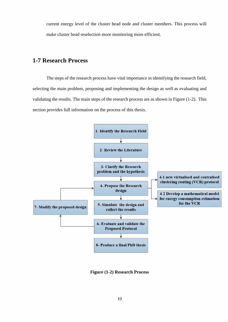
1-7 Research Process
The steps of the research process have vital importance in identifying the research field,
selecting the main problem, proposing and implementing the design as well as evaluating and
validating the results. The main steps of the research process are as shown in Figure (1-2). This
section provides full information on the process of this thesis.
Figure (1-2) Research Process
11
1- Identify the Research Field
The first step of the process is to define the general field of this research. The research
begins by carrying out a detailed analysis of the energy consumption problem in WSN, and the
domains in which the sensor nodes consume energy, as well as which of these domains consume
most energy, and how it should be modified to prolong the network lifetime
2- Review the Literature
This step provides the fundemantal knowledge about the research field. Much research
has been reviewed to understand WSN functions, problems and applications, as well as different
types of existing routing protocols, clustering protocols and algorithms had been reviewed in
order to understand their fundamentals.
Furthermore, various mathematical models introduced for WSN were studied and
reviewed to understand which domains should be taken into accounts during the design of the
proposed mathematical model.
In addition to this, the NFV technique is a new network virtualised method to reduce
the network complexity and power consumption. By taking all this into consideration, the main
concept of this research study will be to exploit the NFV concept to minimise the energy
consumption of the sensor nodes and improve network lifetime.
3- Clarify the Research Problem and the Question
The research problem that defined in the first step is broad in scope. In this step, the
problem was clarified by narrows the scope of the study. As mentioned previously, the network
lifetime and how to improve it is the main objectives in the design of any WSN’s clustering
routing protocols. In addition to this, the power consumption in the clustering based protocol is

12
reviewed in order to understand how the nodes consumes their power during the operation of
the clsutering protocols and how it can be managed in order to improve the network lifetime.
4- Propose the Research Design
Based on the research problem and hypothesis, a research design has been proposed in
order to achieve the aim and objectives. It is divided into two phases:
4-1 Propose a New Virtualised and Centralised Clustering based Routing Protocol
for the Research Idea.
In this phase, a new virtualised and centralised clustering protocol is proposed. In the
proposed protocol, the NFV server will be responsible for implementing the clustering
function. Its operation based on two main steps: the neighbour discovery step, which will
be used to send the sensor nodes’ information to the server via the sink; and the clustering
step, which will be implemented in the NFV server. The clustering step will be divided
into the setup stage (the cluster formation and the cluster head selection) and steady state
stage (data transmissions). Besides this, the k-means clustering algorithm is used to form
the final clusters. The selection of the cluster head is based on a particular cost function,
which is the combination of nodes distance to sink and its current energy level. The full
details of the proposed protocol are discussed in chapter four.
4-2 Develop a Mathematical Model to Estimate the Amount of Energy Consumption
for the Nodes
In order to monitor and manage the network during the protocol operation, a
mathematical model is developed for the proposed protocol in this step. This model will
be used by the server to estimate the amount of energy that will be consumed during the
protocol process.

13
The model takes into consideration the fields that nodes consume their energy in, such as
transmission, receiving, processing, sensing and status change.
5- Simulation of the Proposed Protocol.
This research is based on a simulation experimental and will therefore study and
investigate the amount of energy consumption of the new protocol under different simulation
parameters. In this step, the protocol is implemented and managed using the MATLAB R2016a
simulator.
At the beginning of the simulation, the networks are fed with the necessary information
such as the number of nodes, which are deployed randomly in the simulation environment (the
sensing area with m*m size), the sink (base station) position. As soon as the nodes are deployed,
they will be in stationary mode (fixed position).
The simulation is run under different topologies (randomly deployed) to investigate the
network energy consumption. In addition to that, the number of nodes, the sink position and the
sensing area are used as inputs. These are changed during the simulation to study their effects
on the network and to find the best scenario for the network working in terms of minimum
energy consumption.
The output of the system is the amount of power consumption with different parameters
and finding the optimum number of clusters in terms of minimum power consumption.
Furthermore, the network lifetime is measured based on the first node dead (FND) parameter.
More details on FND are provides in chapter two.

14
6- Evaluate and Validate the Proposed Protocol
The results obtained from the simulation for the proposed protocol is collected and
analysed in this step. Additionally, the protocol is validated based on different scenarios such
as changed numbers of clusters and modified implementation parameters
The purpose of the proposed protocol evaluation to determine how far it achieves the
aim of the research; this is done by comparing it with the traditional protocol (LEACH) and
LEACH-C to find the difference between the results.
7- Modification to Improve the System.
During the simulation process, and if the amendment is necessary to improve the
performance of the proposed protocol to minimise the energy consumption, this step is used to
modify the protocol according to the evaluation of the results.
8- Produce a Final PhD Thesis.
The final step will involve making conclusions and recommendations, then present the
complete PhD thesis.
1-7 Thesis Layout
The remainder of the thesis is organised as follows:
- Chapter 2 outlines the concept of WSN, its applications, sensor nodes architecture,
WSN protocol stack, the energy problem in WSN as well as reviewing an explanation
of the routing protocols, the design requirement of the routing protocol, and the
classifications.

15
- The detailed information about the clustering technique is been explained in Chapter 3.
Furthermore, the main classification for the available clustering protocol, which is
distributed, and centralised clustering protocols had been introduced and various types
of available protocols in both types has been described.
- The full description, assumptions and general steps for the proposed protocol are present
in Chapter 4.
- The mathematical model and the final equations that will be used to measure the amount
of energy consumption in the proposed protocol will be reviewed in chapter 5.
- Chapter 6 describes the simulation experiments of the research, which based on
MATLAB simulator. It include the network parameters, topology and experiments.
Furthermore, validating and evaluation results had been explained in this chapter
- Finally, Chapter 7 contains the main conclusions and future works.

16
Chapter Two
An Overview of Wireless Sensor Networks
2-1 Wireless Sensor Networks Background
Wireless Sensor Network (WSN) represents a class of network technology that is
becoming increasingly popular today. WSNs are used to control and monitor the environment,
and they contain thousands of sensors that communicate with each other to perform a particular
task. Sensing is a technique that is used to collect information about a particular phenomenon
or environment (Dargie & Poellabauer, 2010).
A sensor node forms the main unit of a WSN, which is used to measure changes in the
environment such as vibration, temperature, pressure, humidity, noise and pollution. These
sensor nodes are deployed randomly and in large density (Akyildiz et al., 2002a; Kalantary &
Taghipour, 2014; Potdar et al., 2009).
The functions of these sensor nodes are transmitting the data, processing it and then
communicating with each other to forward it to a central node, which is known as a base station
or a sink via shared wireless channels. The sink either uses the data locally (sends it to users)
or forwards it to other networks (such as the Internet) (Akyildiz et al., 2002a).
The main components of standard Wireless Sensor Network (WSN) are shown in Figure
(2.1) and consist of:
1- Sensing area that can be considered as the field where the nodes will be deployed.
2- Sensor nodes, which represent the main part of the network and the heart of it and are
responsible for sensing activities.

17
3- Sink or Base Station, which is the node responsible for control of the network and its
high proprieties node with no limited resources. The sink acts as a gateway between the
sensor nodes and the outer world. The sink needs to be in a good position because all
the nodes communicate with it for network operation, and in general, the sink is assumed
to be static and does not move in most of the available applications, except for some
applications where the sink needs to move to collect data from the nodes.
Figure (2-1) Simple Diagram of a WSN
At the beginning of designing this network, the communications were based on the
concept of IEEE 802.11; later on, owing to the high power overload of this standard, it became
clear that it was unsuitable for use with this network. Therefore, the new IEEE 802.15.4
standard, which is designed for short-range transmissions and low power sensor nodes, was
utilised in the design of various commercial and academic sensor nodes (Dargie & Poellabauer,
2010).

18
Although this network is a type of ad hoc network, there are various reasons why the
protocols designed for ad hoc cannot be used in the WSN. For instance, the number of sensor
nodes in the WSN is huge, and this requires more scalability management. The sensor nodes
are deployed once and in stationary mode, except for some applications that require mobility
nodes. In ad hoc, however, the nodes are moving all the time. Moreover, the sensor nodes in
the WSN have limited capabilities, such as in processing and energy constraints, and are also
prone to failure. The overhead of the communication for network configuration is also too high,
and in the WSN, the nodes use broadcasting during the operation while in the other ad-hoc
network such as MANET, the nodes use the peer to peer communication. As a result,
minimising energy consumption is the most significant problem in the design of the WSN
(Gowrishankar, Basavaraju, Manjaiah, & Sarkar, 2008).
The design of WSN has special requirements such as power limitations, processing
abilities, memory, fault tolerance, scalability, hardware constraints, transmission media,
environment, deployment process, Quality of Service (QoS) and security (Akyildiz et al.,
2002a; Potdar et al., 2009; Singh & Arora, 2013; Yick, Mukherjee, Ghosal, & Dipak, 2008).
2.2 Wireless Sensor Networks Characteristics
WSN characteristics are different from other types of wireless networks because it is an
application dependent and changeable based on the network design; some of its features are
(Akyildiz, Su, Sankarasubramaniam, & Cayirci, 2002b; Potdar et al., 2009; Singh & Arora,
2013; Yick et al., 2008):
1. Energy Constraints: the network lifetime relies on the energy level of the nodes, so the
power limitation of the nodes becomes the most important design issue in WSN. As the

19
nodes are battery powered, and the nodes are deployed in an unreachable environment,
it is thus hard to replace the nodes’ batteries or charge them with additional energy.
2. Limited resources: owing to the sensor nodes’ small size and battery power, the
processing ability is limited, as well as memory storage and lifetime.
3. Deployment: the deployment of sensor nodes in the network is application dependent
and random. It has two types predetermine and post determine. In the predetermined
type, the nodes deploy either dropping from a plane or are placed in the sensing field
one by one by a human or robot. For the post deployment, there is a change in the
topology by changing nodes’ position and their abilities.
4. Fault tolerance and topology control: the fault of the sensor network should not affect
the performance of the WSN function and should have the ability to change the topology
map in case of any failure. This failure may be caused by various factors such as lack
of power, physical damage and environment interference.
5. Application dependent: the characteristics are different from one application to another,
so the protocols and algorithms for it are application specific.
6. Scalability: depending on application requirements, the number of sensor nodes may be
increased or decreased. Therefore WSN performance should be continuous if new
sensor nodes are added or removed.
7. Security: security is considered a major factor in WSN design to ensure application
processing. Confidentiality, availability, integrity, authentication, authorization and
others represent various security parameters. For instance, if the WSN is used in the
military application, it requires a high level of authentication.
8. Reporting types: in WSN, data reporting categories are continuous, event based, query
based or hybrid. In continuous types, the nodes send their data to the sink periodically
and are based on the predetermined time slot; this is used in temperature sensing

20
applications. This type is considered to be the most energy-saving, as the nodes turn the
radio to on only on their time slot. Event based types are commonly used in critical
applications. The nodes operation here depends on a specific event to start working. For
those applications that require data, when the nodes send their information based on a
request from the sink, this type is known as query based data reporting. The data
reporting this model has a higher priority than the previous two models. Finally, the
combination of the three models is called the hybrid model.
9. Mobility: the nodes in this network may or may not have mobility properties. In general,
most of the available designs of this network consider the nodes to have a fixed position.
However, some applications require the nodes to be mobile and change their position
based on specific conditions.
10. Production Cost: the main part of the WSN is the sensor node. Therefore, the cost of the
single nodes has a significant impact on the design cost of the whole network.
To understand the fundamentals, architecture, design issues, connectivity schemes and
problems of this type of network. Akyildiz et al. (2002a) introduced full studies and surveys in
this field, providing the necessary background required for understanding this network type and
its limitations. Furthermore, in order to understand the WSN architecture, a brief background
on WSN architecture based in OSI model was introduced in (Alkhatib & Baicher, 2012).
In order to summarise the design limitaition and chalalnges in WSN, (Singh & Aloney,
2015) focusing on the general limitations and challenges of WSN that provide the necessary
information regarding to the design of this network.
Some of the design issues that arise in the context of wireless sensor networks were
reviewed by (Sahni & Xu, 2004), specifically, coverage, deployment, and routing algorithms.
The problem of localisation had been introduced and addressed in different research fields;

21
various techniques of node localisation discovery were raised by Pal (2010) who discussed the
future directions and challenges to improve localisation techniques in WSN.
2-3 Sensor Nodes Architecture
Sensor nodes are considered to be the main part of WSN, and they are used for sensing,
processing and sending the data to the central nodes (sink). There are different types of sensor
nodes such as thermal, seismic, infrared and acoustic that are used to sense different
environment conditions such as vibration, temperature, pressure, noise, humidity, pollution,
radiation, and the characteristics of the objects such as speed and the direction (Hu & Cao,
2010).
The sensor nodes contain various components as shown in Figure (2-2) and described
in the following:
1- Sensing unit: this unit consists of sensors and analogue to digital converters. The sensor
can be analogue or digital, and it is used to sense the environment and convert the data
using ADC into a signal to be usable in the network.
2- Processing and storage units: the processor contains a microprocessor that is used to
control and execute the protocols and algorithms; for the storage unit, it can be used to
store the sensing data, and it is optional and depends on nodes’ model and
characteristics.
3- Transceiver units: in this unit, the radio system is used in the communication mode with
neighbours.
4- Power supply unit: the battery represents the main part of this node; it provides the
necessary power to the node and has the main responsibility of the node’s lifetime, but
because the node size is small, the size of the battery is limited.

22
Based on the application type, some sensor nodes contain location units that define
their position. In some conditions, it is necessary for the nodes to know their position; for
instance, in tracking or event-based applications, the nodes should provide the location of the
events with the sensing information.
Additionally, a mobilised unit enables the sensor nodes to move in the sensing area
based on the sensing task that they perform.
Figure (2-2) Sensor Node’s Architecture
2-4 Wireless Sensor Network Applications
The wireless sensor networks can perform various types of high-level applications such
as in military operations, health, environment and home monitoring. These applications help to
investigate and understand the environment situation easily.

23
WSNs have the ability to perform many applications that help people to examine and
understand the sensed environment easily. The application can be classified according to the
reporting type, such as event-based, query based and time-driven based.
There are various types of sensor network applications, and they depend on application
requirements such as deployment method, mode of sensing, type of power supply and others
(Zhao & Guibas, 2004).
WSN applications are categorised into tracking applications and monitoring
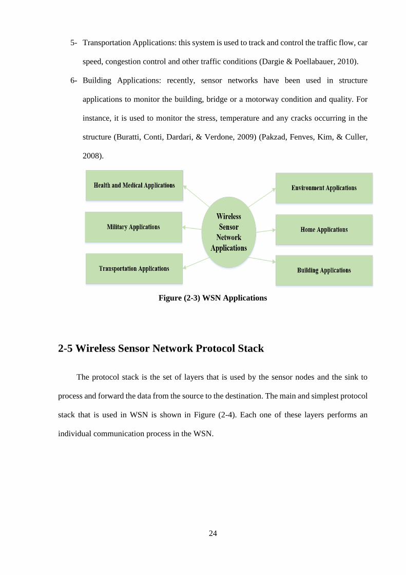
applications. Various types of WSN applications are shown in Figure (2-3). This section will
briefly introduce different types of these applications.
1- Military Applications: WSN has an important role in the military field. This network
can be used for tracking and monitoring military forces and enemy forces, equipment
and battle areas (Akyildiz et al., 2002a).
2- Health and Medical Applications: WSNs can be utilised in the health field to monitor
patients, such as their blood pressure and heart rate and tracking their movement without
the need to stay at the hospital. In addition to this, it can be used to track the doctors’
movements (Abidi, Jilbab, & Haziti, 2017) (Dargie & Poellabauer, 2010).
3- Environment Applications: this application represents the first application that was
implemented by WSN, as it was used to monitor the environment situation such as
seismic system, flood detection, pollution, climate, temperature, humidity, light and
pressure as well as monitoring environmental resources such as soil and water quality.
In addition to that, it is used in animal tracking and monitors behaviour. WSNs have
been widely applied in this type of application (Rajaravivarma, Yang, & Yang, 2003).
4- Home applications: sensor nodes can be used to help people monitor and manage their
home devices via a network or the internet (Sadhana, Malik, Gogia, Devi, & Chhabra,
2013).
24
5- Transportation Applications: this system is used to track and control the traffic flow, car
speed, congestion control and other traffic conditions (Dargie & Poellabauer, 2010).
6- Building Applications: recently, sensor networks have been used in structure
applications to monitor the building, bridge or a motorway condition and quality. For
instance, it is used to monitor the stress, temperature and any cracks occurring in the
structure (Buratti, Conti, Dardari, & Verdone, 2009) (Pakzad, Fenves, Kim, & Culler,
2008).
Figure (2-3) WSN Applications
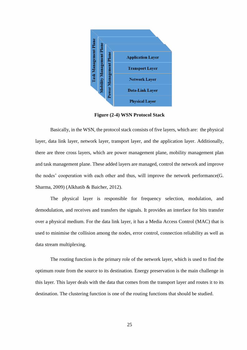
2-5 Wireless Sensor Network Protocol Stack
The protocol stack is the set of layers that is used by the sensor nodes and the sink to
process and forward the data from the source to the destination. The main and simplest protocol
stack that is used in WSN is shown in Figure (2-4). Each one of these layers performs an
individual communication process in the WSN.
25
Figure (2-4) WSN Protocol Stack
Basically, in the WSN, the protocol stack consists of five layers, which are: the physical
layer, data link layer, network layer, transport layer, and the application layer. Additionally,
there are three cross layers, which are power management plane, mobility management plan
and task management plane. These added layers are managed, control the network and improve
the nodes’ cooperation with each other and thus, will improve the network performance(G.
Sharma, 2009) (Alkhatib & Baicher, 2012).
The physical layer is responsible for frequency selection, modulation, and
demodulation, and receives and transfers the signals. It provides an interface for bits transfer
over a physical medium. For the data link layer, it has a Media Access Control (MAC) that is
used to minimise the collision among the nodes, error control, connection reliability as well as
data stream multiplexing.
The routing function is the primary role of the network layer, which is used to find the
optimum route from the source to its destination. Energy preservation is the main challenge in
this layer. This layer deals with the data that comes from the transport layer and routes it to its
destination. The clustering function is one of the routing functions that should be studied.

26
For transport layer, the primary role is to provide reliability to control and minimise the data
flow in the network based on the application requirements, to provide end to end reliability and
security.
The last layer on the top is the application layer, which has the responsibility of
representing the required data used software to the users, such as sensor network management.
WSN is used in different applications in various fields such as military, medical and
environment.
However, the crossover layers have different management functions. The power plane
layer is to manage and controls sensor nodes’ power usage. In addition, it manage how the
nodes can monitor their energy consumption during the performance of different operations
such as sensing and communications. In the contrast, the mobility plan layer manages the
mobility and movement of the nodes. Also, the sensing and data sending process are controlled
and scheduled by the task plane layer (Mir, 2014; Sharma, 2009) (Al-Obaisat & Braun, 2007).
Now, in order to understand the routing function, the next section contains the necessary
information about what routing means, the routing protocols classifications, and the available
routing protocols and algorithms.
2-6 Routing Protocols in WSN
Routing considers the primary function of the third layer of the protocols stack model
(network layer). The routing process is the process of forwarding data from the source (sensor
nodes) to destination (sink). Depending on the sensor nodes transmission range, the
communication process may occur directly to the sink (single-hop model), and it is like a star
topology or via an intermediate node(s) (multi-hops model) forming a mesh topology as
illustrates in Figure (2-5) (Dargie & Poellabauer, 2010).

27
The functions of the routing process in sensor nodes include establishing a connection
with adjacent nodes to exchange information, building a routing table and sharing it with other
nodes and calculating the best route. The implementation of these functions is achieved using
routing protocols and algorithms (Al-Karaki & Kamal, 2005).
(a) Single Hop (b) Multi-Hop
Figure (2-5) WSN Communications type
The routing protocols and algorithms are sets of rules that manage the connection
between two nodes, control the data transmission from one sensor node to another and calculate
the best path to forward data from source to destination depending on certain metrics.
Routing protocols face difficult challenges in the design of WSNs because of their
features that make it different from the available types of wireless networks such as MANET.
Firstly, in WSN it is impossible to use traditional IP-addressing because of the massive numbers
of sensor nodes. IP is used in reliable concoctions (such as cables or fibre optics), and the data
error rate is uncommon while in WSN the connection between nodes is wireless, so the error is
expected all the time. Thus, traditional networks’ protocols cannot be adopted in WSN. Second,
all applications in WSN require the transmitted data from multi sources to a single destination
(sink). Furthermore, sensor nodes have limited resources such as transmission power,
processing capacity and storage so the routing process should manage these resources carefully

28
(Akkaya & Younis, 2003) (Al-Karaki & Kamal, 2004). According to these characteristics,
various types of routing protocols and algorithms have been designed and proposed to
implement data routing in WSN.
In WSN design, the routing protocol has been a focus in the research field. Routing
protocols and algorithms are application-dependent, and their requirements differ from one
application to another; for instance, protocols’ characteristics for environment monitoring
applications are distinct from that needed for military use (Akkaya & Younis, 2003)
(Eslaminejad & Razak, 2012) (Villalba, Orozco, Cabrera, & Abbas, 2009).
The routing communication method in WSN can be classified into the sink to nodes and
nodes to sink. It depends on the type of protocol used in the network. For the first category, the
sink is responsible for starting the communication process. It is subdivided into the sink to all,
sink to one and sink to the group (Chen, Li, Ye, & Wu, 2007). For the nodes to sink, they are
used in the data-centric system or networking system. This type has more overhead on node
storage, energy and packet control than other types.
2-6-1 Design Requirements for WSN Routing Protocols
As mentioned previously, the sensor nodes have limited battery and processing, and
therefore, to design routing protocols and algorithms in WSN, the following requirements
should be considered (Al-Karaki & Kamal, 2004; Khurana, 2013; Sharma, 2009):
1- Energy Consumption: this factor depends on the nodes’ battery, as the sensor node’s failure
causes topology changes, rerouting the data and network’s reorganisation. To achieve this, the
routing technique reduces the number and the size of data that will transfer (Mundada, 2012).

29
2- Node deployment: this is application dependent. The node deployment may be deterministic
(sensor nodes are manually deployed, and their paths are predetermined) or randomise (sensor
nodes deployed randomly).
3- Data reporting models: in WSN, sensed data sending from the sensor nodes can be
categorised into continuous, event-based, query based and hybrid. In the continuous model, the
sensor nodes send their data to the sink periodically at a particular defined rate. In the event-
based model, the sensed data sending depends on the event detected. For query based, the sensor
nodes send their data only when they receive a query from the sink. Finally, the hybrid model
is a mix of the three mentioned models.
4- Fault tolerance: the network should not be affected by any sensor node failure, and that which
is achieved by routing protocols should find alternative solutions.
5- Scalability: routing protocols and algorithms should have the ability to manage and control
any change in the numbers of sensor nodes; this change may happen by adding or removing
sensor nodes to/from the network.
6- Network dynamics: it is application dependent. Sensor nodes and the base station may be in
either stationary mode (fixed position) or mobility mode (dynamic position).
7- Connectivity and coverage: this depends on the deployment of the sensor nodes.
8- Data aggregation: this means data collection from different resources and sends it as one
packet in order to achieve energy efficiency.
9- QoS: this is application dependent because in some applications, data should be delivered
within specified times or it will be useless. On the other hand, saving network energy is more
important that data quality.

30
10- Topology change: the network topology may change because of many reasons, such as node
damage and link failure.
11- Node homogeneity/heterogeneity: this is application dependent. Homogeneity sensor nodes
mean that all nodes have equal rules in computation, energy consumption and communication.
Moreever, heterogeneity refers to the differences in sensor nodes’ rules.
12- Applications dependent: the design of routing protocols is application specific, which
means that the routing characteristics are based on the network design requirement (Singh &
Sharma, 2015).
2-6-2 CLASSIFICATION OF ROUTING PROTOCOLS IN WSN
The routing protocols in this network can be classified according to different parameters
such as node location, node functionalities and other parameters; this section will illustrate a
review of these classifications and their types. Figure (2-6) summarises the classification of
routing protocols and algorithms.
Figure (2-6) Routing Protocols Classifications
31
2-6-2-1 Network structure-based Routing Protocols
The network structure category divided into flat, hierarchy and location based routing
protocols ( Singh, Singh, & Singh, 2010) (Cecílio et al.) (Al-Karaki & Kamal, 2004, 2005), as
follows:
I. Flat Routing Routing Protocols
All sensor nodes have the same functionality in flat routing protocl, as well as the
communication, depend on sink query. The sink sends a query to a particular region and
waits for a response from it. As it is query based, attribute-based naming is using for the
data requested. There are different protocols, and algorithm examples include flooding,
gossiping, Sensor Protocol for Information via Negotiation (SPIN), and Direct
Diffusion.
II. Hierarchical and Clustering Routing Protocols
The main goal of Hierarchical and clustering is to reduce energy consumption by
dividing the sensor nodes into clusters, and for each one there is a cluster head, which
is responsible for managing and controlling all sensor nodes within it. Examples of this
type are LEACH, Power-Efficient Gathering Algorithm in Sensor Information System
(PEGASIS), Threshold-Sensitive Energy-Efficient Protocol (TEEN) and Adaptive
Periodic TEEN (APTEEN). Full details of these categories are described in the next
chapter.
III. Location-based Routing Protocols
The protocols classified under this category depend on sensor nodes’ location
information. This location information can be found by communication between nodes
or directly by using GPS techniques if the sensor node has a GPS receiver. This type is
32
also considered to be an energy saver because it allows the nodes to switch to sleep
mode if there is no activity with it. Geographic Adaptive Fidelity (GAF), Energy Aware
Greedy Routing (EAGR), and Geographical and Energy-Aware Routing Protocol
(GEAR) are examples of this type.
2-6-2-2 Protocol Operation based Routing Protocols
Routing protocol in WSN has another important category that is based on the network
operation. In this category, the protocols are performed based on the network requirement or
what the network needs to operate based on a particular change. The operation-based category
is organised into:
I. Query-based Routing Protocols:
The operation of the protocols based on a query where the sink or destination node
broadcasts a data request to all nodes in the networks. The sensor node will check if the
query matches their sensed data or not, and if there is a match, the nodes send the required
data to the sink or the requested nodes. Direct Diffusion and Rumour Routing are classified
under this type.
II. Multipath-based Routing Protocols:
In the Multipath-based category, the protocol uses multipath to the sink to achieve high
performance. The sensor nodes establish multipath from the source to destination, and this
will increase the network reliability and performance and enhance its lifetime. Furthermore,
the node can use the other paths to distribute their traffic between them. The best examples
of this type are Directed Diffusion and Energy-Aware Routing Protocol.
III. Negotiation-based Routing Protocols:
The operation of the protocols is based on a negotiation process. The nodes use a high-level
data descriptor instead of the full data during the protocol process to eliminate the redundant

33
data. After completing the negotiation process and establishing a connection to the required
node, the actual data will be sent. The general example of this type is SPIN.
IV. QoS based Routing Protocols:
The protocol should have the ability to balance between data QoS requirements such as
delay, sample rate, data accuracy, sufficient bandwidth and energy. The protocols in this
type enable the nodes to make a trade-off between the energy consumption metric and
various QoS metrics. Examples of this kind are SPEED (Stateless Protocol for Real-Time
Communication in Sensor Networks) and SAR (Sequential Assignment Routing).
V. Non-Coherent and Coherent Based Routing Protocols
In non-coherent based routing, the data will be processed in the node before sending it to the
aggregator for further processing. Data processing is achieved in three stages; the first stage
includes target discovery, data gathering and data pre-processing, while the second phase
confirms the connections, and finally, in the third stage the central node will be selected. An
example of this type is Single Winner Algorithm (SWE).
However, in incoherent based routing, the level of data processing in the node before sending
to an aggregator is limited. The limited processing includes time stamping, duplicating
suppression and other. This type is the best choice to use in the energy efficient routing. An
example of coherent based routing is Multiple Winner Algorithm (MWE).
2-6-2-3 Routes Establishment
Routing protocols can be classified according to paths calculation process within the
network to trasmite the data from the node to the base station. The routes computations
classified as follows:
34
I. Proactive Routing Protocols:
In this type of protocol, the nodes build their routing table to find the route to the destination
before needed. The delay in this kind is minimising because the path is ready to use, but at
the same time, the bandwidth may increase because of the updated information in the routing
table. It is suitable for real-time applications. Examples of this type are Wireless Routing
Protocol (WRP) and The Topology Dissemination Based on Reverse-Path Forwarding
Protocol (TBRPF).
II. Reactive Routing Protocols:
Demands under these protocols determine the routing tables. It does not need to update the
information because the table is already up-to-date, but the delay will increase because the
tables are not ready and it should be determined. Examples of this type are: Temporarily
Ordered Routing Algorithm (TORA) and Energy-aware Temporarily Ordered Routing
Algorithm.
III. Hybrid Routing Protocols:
The protocols in a hybrid are a combination of the properties of the proactive and reactive
protocols. This combination occurs because of the communication process between the
sensor nodes, which are located in the same area and are therefore near to each other. At the
same time, the topology’s changes are significant if the nodes are close to each other and
will not affect other parts of network Zone Routing Protocol (ZRP).
Various research and surveys have been carried out in the field of routing protocols in
WSN. Full studies of the routing protocols and their classification have been introduced by
(Akkaya & Younis, 2003) (Al-Karaki & Kamal, 2004) (Cecílio et al.) (Parvin & Rahim, 2008)
(Singh et al., 2010) (Sumathi & Srinivas, 2012). The major factors in the design of routing
protocols and the characteristics for each one have been discussed by (Biradar, Patil, Sawant,
& Mudholkar, 2009) (Dekivadiya & Vadharia, 2012).

35
A study by Ramya, Saravanakumar, & Ravi (2016) provided a review of the importance
of the energy efficiency routing protocol in the design of wireless sensor network and of
enhancing its lifetime; they introduced the available routing protocols as a classification and
reviewed the characteristics for each of them.
The available energy efficient routing protocols were studied and discussed in (Devi &
Sethukkarasi, 2016). They classified these protocols into different classifications and compared
them based on the main parameter that should be taken into account in any routing protocols
design.
Among all classifications of routing protocols, the clustering based protocols are the
most popular when considering sensor nodes’ energy saving. The idea of these protocols is
based on dividing the network into clusters, which will be responsible for transferring data
between sensor nodes and the sink. The communication with the sink is done via a head node,
which is known as the cluster head. Various routing protocols can be classified as clustering-
based protocols. Low-Energy Adaptive Clustering Hierarchy (LEACH) was the first protocol
that used this technique, and Power-Efficient Gathering in Sensor Information Systems
(PEGASIS), Threshold-Sensitive Energy-Efficient (TEEN) Protocol and Adaptive Periodic
(APTEEN) are some further examples of this technique. The next chapter will review the basic
principles of the clustering function.
2-7 Energy Consumption in Wireless Sensor Networks
Increasing the network lifetime is considered a major challenge in the design of sensor
networks. Because of a power source for the nodes is the battery, and the nodes are deployed
in an unreachable environment, the battery replacement process is difficult. Accordingly, the
36
designers should take into account energy consumption as the primary consideration in
designing any algorithms or protocols (Singh & Arora, 2013).
The source of sensor nodes’ power consumption can be divided into useful consumption and
wasteful consumption, as shown in Figure (2-7).
The useful consumption includes:
Communications (including both transmission and receiving): sensor nodes consume
most of their power on communication, especially if nodes are located far away from
the base station.
Sensing.
Data processing.
While the wasteful consumption domains are:
Collision: A collision occurs when some sensor nodes send data at the same time and
on the same channel.
Overhead and overhearing: overhead means that sensor nodes exchange redundant data
while overhearing occurs when a sensor node receives data that are addressed to other
nodes.
Idle/sleep: if the sensor node is in idle mode (not receiving or transmitting any data), it
will consume energy. Therefore, power management approaches are used to switch off
the nodes when not in use.
Over-emitting: a sensor node consumes energy sending the data, and the destination is
not ready.
Different factors affect the power consumption of the sensor nodes; these factors were
introduced in (Kumar & Singh, 2016). The authors stated that some of these factors are
communications, collisions, idle and listening modes.

37
Figure (2-7) Energy Consumption Domains
The highest amount of energy is consumed in the communication field. For example,
and based on the research; the power consumption for processing approximately 3000 coded in
the processor units is equal to the energy that is consumed to transmit 1 bit of data. Therefore,
managing the communication field is necessary to improve the network lifetime (Pottie &
Kaiser, 2000) (Ahmedy et al., 2011) (Ali & Roy, 2008) (Anastasi et al., 2006) (Rezaei &
Mobininejad, 2012).
One of the primary issues in the design of WSN is the energy management and how its
consumption can be minimised. Shaikh & Zeadally (2016) proposed a taxonomy of the
available energy harvest sources that can be used in the design of WSN. In addition to that, the
paper introduces a review of the available energy models used in energy harvest.
In general, as mentioned previously, the node consists of various components such as
transceiver, processor and sensors, and each one of these components has its modes; for
instance, in the case of the sensor component, as shown in Figure (2-8), there are only two
modes - on an off. The transceiver component that contain the receiver and transmitter have
four modes: transmit mode, receive mode, idle mode and sleep mode as illustrated in Figure (2-
9). On the other hand, Figure (2-10) represents the processing component, which has three
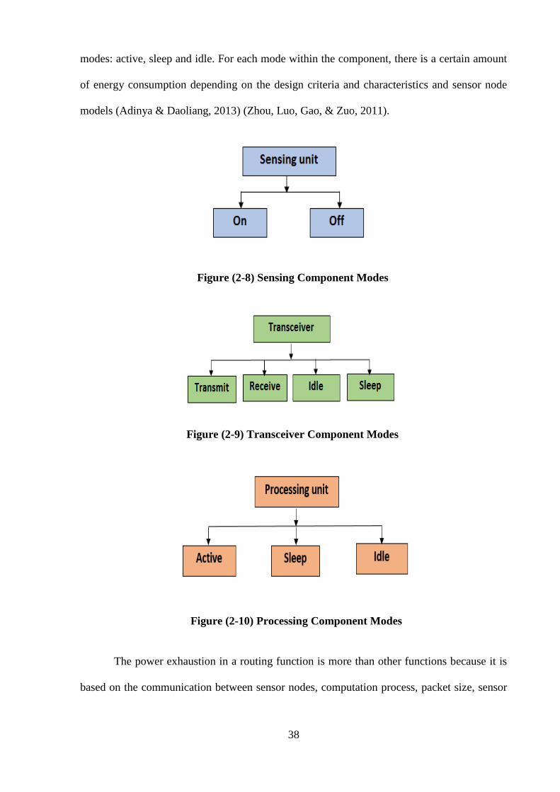
38
modes: active, sleep and idle. For each mode within the component, there is a certain amount
of energy consumption depending on the design criteria and characteristics and sensor node
models (Adinya & Daoliang, 2013) (Zhou, Luo, Gao, & Zuo, 2011).
The power exhaustion in a routing function is more than other functions because it is
based on the communication between sensor nodes, computation process, packet size, sensor
Figure (2-9) Transceiver Component Modes
Figure (2-8) Sensing Component Modes
Figure (2-10) Processing Component Modes
39
nodes status and the distance between sensor nodes and the sink. The aim of most researches
has been to find schemes to increase network lifetimes. Some of these plans reduce the number
of communications, by minimising the packet size, using efficient duty cycle mechanisms,
optimising neighbour selection and reducing the distances that control the on and off status of
sensor nodes.
A new energy conservation scheme was proposed by (Pantazis, Vergados, Vergados, &
Douligeris, 2009) (Pantazis, Nikolidakis, & Vergados, 2013). This system was based on
reducing the end-to-end delay. The researchers recommended using it with a network that
monitors rare events and operates for a long time. In addition, (Anastasi, Conti, Di Francesco,
& Passarella, 2009) introduced a classification of energy saving methods such as data based
and duty cycling based.
The energy saving methods in WSN were presented by (Ali & Roy, 2008). The
conservation methods have been classified according to node level, network level and software
level. Packet size optimisation have also been used to enhance energy consumption in wireless
sensor networks.
However, there are different surveys, which were introduced in this area, such as a study
of power saving and energy optimisation techniques as presented in (Sendra, Lloret, García, &
Toledo, 2011), where the authors presented the available methods used to reduce the energy
consumption in WSN and increase network lifetime.
Meanwhile, the sensor node energy consumption was analysed and introduced in
(Sharma, Shinghal, Srivastava, & Singh, 2011), and the mathematical model presented in this
paper depends on a proposed sensor node with its characteristics. The results of this model are
used to estimate the approximate lifetime of the node. In addition to this, the researchers
investigate the amount of energy consumption of the transceiver part of the sensor node.

40
In routing, routing protocols and algorithms can use these schemes to achieve energy
efficiency in networks (Thangadurai & Dhanasekaran, 2013), and energy harvesting has been
the objective of much research in this field. (Anastasi et al., 2006) Discussed various approaches
such as supplying energy from external sources or saving energy using efficient protocols and
algorithms that can save sensor nodes’ battery life. A study of sensor nodes’ power management
was carried out by (Ahmedy et al., 2011).
Energy gains significant attention during the design of new protocols and algorithms in
the routing process. The communications among sensor nodes, the packet size, the distance
between sensor nodes, the sink, and the sensor nodes' idle mode are the main sources of power
dissipation in routing. There are various types of routing protocols whose primary design factor
is reducing energy consumption, such as Low Energy Adaptive Clustering Hierarchy
(LEACH), Sensor Protocols for Information via Negotiation (SPIN) and Energy-aware routing
protocol (Cecílio et al.).
2-7-1 Sensor Node and Network Lifetime
The sensor node’s energy level had a significant effect on the Network lifetime, which
is an important performance metric in Wireless Sensor Networks (WSNs).
There are three principal ways to determine the network lifetimes (Tian & Georganas, 2002)
(Madan & Lall, 2006):
1- The time duration between the start of communication and the time when the first node
dies (FND).
2- The time duration between the start of communication and the time when the half of the
nodes die (HND).
3- The time duration between the start of communication and the time when the last of the
nodes die (LND).

41
On the other hand, the authors in (Xue & Ganz, 2006) introduce another idea, which is
that the lifetime is based on the specified percentage of the dead node, for example when the
number of dead nodes reaches the assumed rate; this means that all nodes are dead.
This thesis aims to evaluate the protocol, and the First Node Dead (FND) is the main
parameter that will be adopted.
2-8 Summary
From the research conducted, it is clear that a significant development has been
occurring in the design of WSN. This network consists of small and battery powered nodes with
limited resources (limited energy and memory) cooperating with each other to perform a
particular sensing task, and because of the sensor nodes’ energy limitations, power management
has become an essential factor to be considered during the design of the protocols.
There are various issues concerning the design of this type of network, for instance, the
energy constraints, communications among the nodes to perform a task, delivery mode,
application type and nodes deployment process.
A brief introduction of wireless sensor networks, sensor nodes’ overall architecture,
protocol stacks, and routing protocols have been discussed in this chapter. Various types of
applications and energy consumption fields in this kind of network have also been reviewed in
this chapter.
Furthermore, the definition of routing protocol and its classifications have been
provided. In addition, the sensor nodes units that consume energy in different modes such as in
transfer, receive and idle, have also been reviewed in detail in this chapter. Finally, this chapter
has introduced the main points regarding routing protocol design requirements in WSN, which
have been taken into consideration through this research process.

42
Chapter Three
Literature Review of Clustering Based Routing Protocols
in Wireless Sensor Networks
3-1 Introduction
The limited resources of sensor nodes introduce challenges to the design of any routing
protocols. By minimising the energy consumption of the nodes, the network lifetime should be
improved. However, the clustering function is the most important routing function that should
be managed. During the operation of clustering based routing protocols, the sensor nodes
consume a significant amount of energy during the implementation of clustering stages. These
cluster-based routing protocols are categorised into distributed types, where the nodes are
responsible for clustering functions, and centralised types, which are used to improve the
distributed clustering protocols. In protocols that are based on a centralised process, the base
station is responsible for clustering functions.
In this chapter, the main definition and challenges in clustering approach are discussed.
Furthermore, a literature review of related work to existing clustering routing protocols in WSN
is presented to be utilised in the design of the proposed protocol in this thesis.
3-2 The Clustering Approach
As mentioned previously, clustering is the process of dividing the sensor nodes into
groups known as clusters, as shown in Figure (3-1). For each cluster, a single node will be
responsible for all functions within the cluster such as aggregation and processing the data

43
before sending it to the sink, this single node known as a cluster head. The cluster head
communicates with the sink directly or via one or multi-hops communications. The main and
important aim of the clustering function is to improve the network lifetime (Zhang, Mamalis,
Gavalas, Konstantopoulos, & Pantziou, 2009) (Pal, Singh, Yadav, & Pal, 2012) (Abbas &
Younis, 2007) (Zhang et al., 2009) (Zhao & Guibas, 2004)
Figure (3-1) Architecture of Cluster-Based Routing Protocols
The clustering function is divided into two stages, the setup stages and steady stages; in
the first stages, the cluster head will be selected, and the cluster will be formed, while in the
steady-state stage the sensor nodes within the cluster will start sensing the data and send it to
the CH that will send it to the sink. Figure (3-2) represents the main stages of clustering.

44
Figure (3-2) Clustering Function Stages
The clusters can be classified based on different properties, as illustrated in Figure (3-3).
Figure (3-3) Clustering Proprieties

45
The following list is to explain the clustering proprieties in details:
1- Static vs. dynamic: the clusters formation and cluster head selection performed only
once in the static clustering. In this type, the cluster head node will consume all its power
and die and thus, will isolate the whole cluster and make it unreachable. In contrast, in
dynamic clustering, the clusters formation and cluster head selection change at each
cycle or round.
2- Heterogeneous vs. homogenous: In heterogeneous, the sensor nodes are different in
their abilities such as in processing and energy level. Therefore, the CH selection will
be based on a node with the highest abilities. However, in the homogenous, all sensor
nodes have to save proprieties, and all of them have a chance to be CH.
3- Distributed vs. centralised: In WSN this type is the most important. The clustering
function implementation can be classified into two main types, the standard and most
popular type are the distributed clustering protocols, which means that the clustering
function performed by the nodes and the sensor nodes are responsible for clustering
decisions. The most popular protocols in this type are LEACH, TEEN, and Hybrid
Energy Efficient Distributed Clustering (HEED), PEGASIS: Power-Efficient Gathering
in Sensor Information Systems. In contrast, the centralised means that there is a central
node/s (generally the sink) responsible for the clustering function. LEACH-C, BCDCP,
and LEACH-F. All the available centralised routing protocol is based on the sink
function (sink responsible for the clustering function). Also, the main drawback of this
technique is the process of sending nodes information that is performed at the beginning
of each round.
4- Probabilities vs. Non- Probabilities: In probabilities clustering, the process of cluster
formation and cluster head selection is based on a random and non-uniform process.

46
However, in non-probabilities, the clustering function is based on pre-determined
parameters such as node ID, node weight or energy level.
Many design issues should be taken into consideration during the design of any
clustering protocol. Some of these problems are the energy constraints and network lifetime.
The methods of cluster head selection and cluster formation have a significant impact on the
overall network performance, and in addition, scalability, network topology, data aggregation,
secure communication, and fault tolerance have important implications for the clustering
methods (Singh & Sharma, 2014) (Kumarawadu, Dechene, Luccini, & Sauer, 2008) (Abbas &
Younis, 2007).
The clusters have different characteristics, which affect the network lifetime such as:
Cluster count: the cluster count is the number of clusters formed in one round, and it
should balance to achieve energy efficiency (Gupta, Jain, & Sinha, 2013) (Pal et al.,
2012).
Cluster size: is the number of nodes within clusters. It is based on the distance between
the nodes within the cluster and should be managed for efficient performance. The
smaller size of the cluster, the better the energy efficiency because the communication
distance is minimised, and it can be fixed or dynamic. The cluster size may be uniform
or non-uniform depending whether the size is the same for all clusters or different
(Gupta et al., 2013) (Kumar, Dhok, Tripathi, & Tiwari, 2014) ( Liu, 2012).
Intra-communication: it represents the communication inside the cluster, between the
sensor nodes and their cluster head that can be single hop or multi-hops, as illustrated
in Figure (3-4a, b) (Gupta et al., 2013) (Kumar et al., 2014).

47
Inter-communication: it represents the communication between the cluster heads and
the base station, and it can be single hop or multi-hops, as shown in Figure (3-4c, d)
(Gupta et al., 2013) ( Kumar et al., 2014).
The cluster head selection approaches can be classified into deterministic, adaptive and
random. In the deterministic, the selection is based on particular parameters such as an identifier
or neighbours’ nodes. In the adaptive approach, the selection of the cluster head is based on a
certain function such as its energy level or communication cost. Finally, for the random type,
the selection is made randomly without regard to any parameters (Liu, 2012).
(a) (b)
(c) (d)
Fig (3-4) Clustering Model
(a- Intra-communication (Single hope), b- Intra-communication (Multi-hop), c- Inter-
communication (Single hope) , d- Inter-communication (Multi-hop))

48
The cycle process of the clustering is divided into rounds, with each round divided into
frames as shown in Figure (3-5). For steady-state stages, the frames will be using the Time-
Division Multiple-Access (TDMA) schedule to set a time slot for each node to use during the
data transmission process (Shigei, Miyajima, & Morishita, 2010).
Figure (3-5) Clustering Timing
The sensor nodes send their information to their cluster head once per frame, and at the
end of this frame this cluster head will aggregate the data and send it to the sink once per frame.
The main drawback of the clustering function is the communications, which is the key
issue in the design of this function domain that includes inter communication between the
cluster head and the sink and the intra communication among the sensor nodes and the cluster
head. Furthermore, the cluster head nodes spend more energy in communications and
calculations, and this is considered an issue in designing any clustering protocols (Singh &
Aloney, 2015) (Patil, Kulkarni, & Ayachit, 2011).
The communication cost is divided into two types: before clustering cost and after
clustering cost. The before clustering cost is the communications that are needed to perform the
clustering function, form the clusters and select the cluster head node, while the after clustering
cost is based on the intra cost of communications. This type is among the sensor nodes and

49
inside the cluster itself, while the inter cost is the communications cost between the cluster head
and the sink. Thus, it is essential to manage these communications costs in order to make the
clustering process more efficient (Tripathy & Chinara, 2012).
(Arboleda & Nasser, 2006) Investigate the concept of the clustering techniques such as
cluster elements, cluster advantages and cluster types, and in addition to that, they introduce a
survey of various clustering algorithms and protocols and list the main differences among them.
In order to understand the different classifications on the clustering algorithms, the
author (Abbas & Younis, 2007) introduces a clustering taxonomy that classified the clustering
algorithms and protocols according to their design objectives such as energy consumptions,
coverage, mobility, position, and load balancing.
The cluster heads selection methods are changeable and different from protocol to
protocol, as summarised in the survey (Thakkar, 2016). In this research, the author focuses on
the hierarchical routing protocols types and reviews the available protocols and their
characteristics for both homogeneous and heterogeneous networks with station nodes to
introduce a full taxonomy of these techniques. Furthermore, various clustering approaches had
been investigated in (Ramesh & Somasundaram, 2011). The authors reviewed the exiting
algorithms based on their costs in cluster head selection, transmission as well as the requirement
for the cluster head rotation. It concludes that the available algorithms need more study in terms
of scalability and energy efficient in WSN.
A taxonomy of the clustering algorithm was introduced in (Singh & Sharma, 2015). In
this paper, the metrics and the limitations of the clustering functions were described, and the
authors proposed future work be done in the field of clustering in WSN.
Regarding the mobile WSN, the (Sabor, Sasaki, Abo-Zahhad, & Ahmed, 2017) studied
and explained some of the available hierarchical and clustering based routing protocols that had

50
been proposed in the last five years. The survey contained a compression between the protocols
based on delay, network size and energy efficiency as well as illustrate the advantage and
disadvantage for each protocol.
In this thesis, the concept of the k-means algorithm is adopted to cluster the network
during the implementation process, and a full explanation of this algorithm is introduced in the
next chapter.
3-4 Clustering Based Routing Protocols
In general, the important classification of clustering based routing protocols is who is
responsible on clustering function; it can divided into distributed or centralised protocols as
illustrated in Figure (3-6). The full details of each category will be described in the next
sections.
Figure (3-6) Clustering Routing Protocols classification

51
3-4-1 Distributed Clustering Protocols
In the distributed protocols, the clustering function is based on the communications
among the sensor nodes to perform the clustering function and manage the network.
Additionally, the nodes are considered to be location-unaware, which means that they do not
have any information about their location and other nodes’ location within the network. Hence,
the clustering decision is based on internal information. According to this, the energy
consumption of the clustering causes an extra overhead regarding communications; this will
maximise the energy consumption of the nodes and affect the network lifetime.
With this type, the available protocols focus on the cluster formation or cluster head
selection techniques. However, regarding the number of communications, the same procedure
is used which shown in Figure (3-7).
Figure (3-7) Distributed Clustering Protocol Flowchart
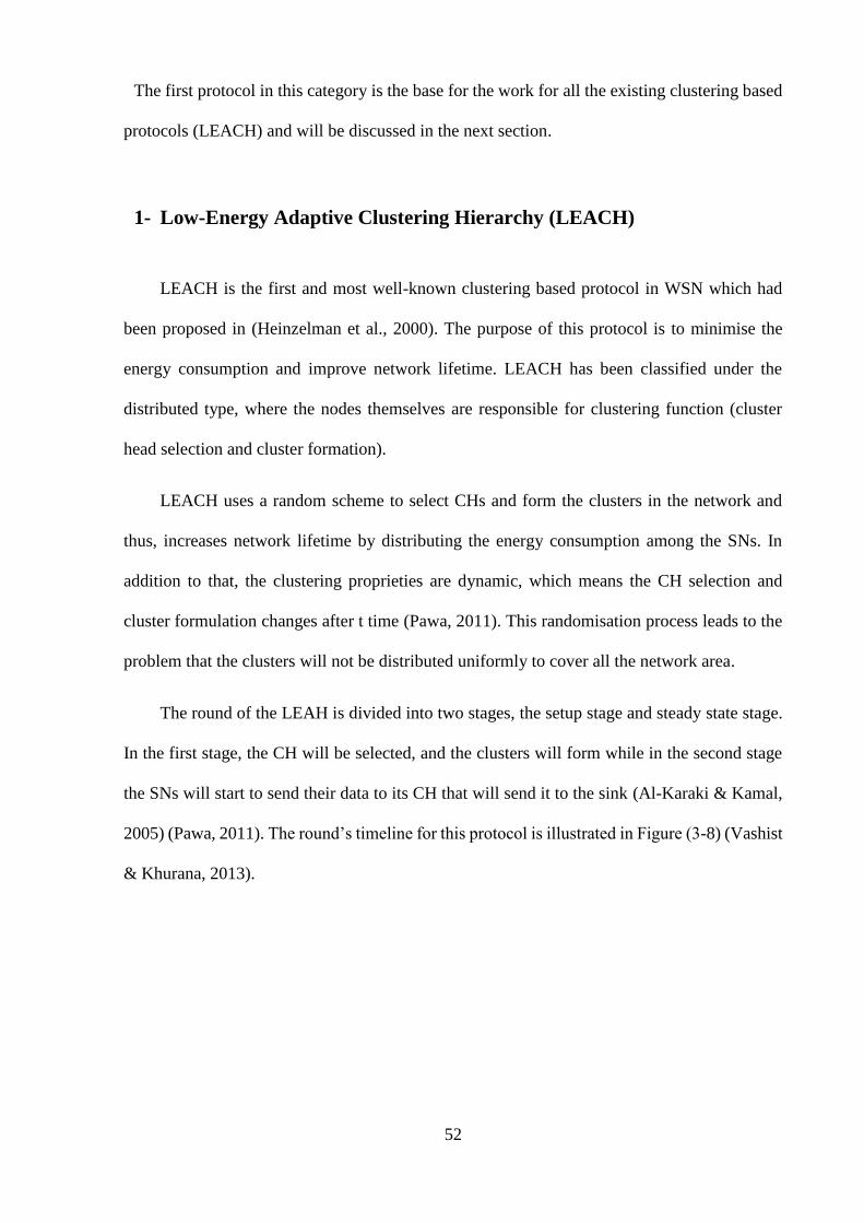
52
The first protocol in this category is the base for the work for all the existing clustering based
protocols (LEACH) and will be discussed in the next section.
1- Low-Energy Adaptive Clustering Hierarchy (LEACH)
LEACH is the first and most well-known clustering based protocol in WSN which had
been proposed in (Heinzelman et al., 2000). The purpose of this protocol is to minimise the
energy consumption and improve network lifetime. LEACH has been classified under the
distributed type, where the nodes themselves are responsible for clustering function (cluster
head selection and cluster formation).
LEACH uses a random scheme to select CHs and form the clusters in the network and
thus, increases network lifetime by distributing the energy consumption among the SNs. In
addition to that, the clustering proprieties are dynamic, which means the CH selection and
cluster formulation changes after t time (Pawa, 2011). This randomisation process leads to the
problem that the clusters will not be distributed uniformly to cover all the network area.
The round of the LEAH is divided into two stages, the setup stage and steady state stage.
In the first stage, the CH will be selected, and the clusters will form while in the second stage
the SNs will start to send their data to its CH that will send it to the sink (Al-Karaki & Kamal,
2005) (Pawa, 2011). The round’s timeline for this protocol is illustrated in Figure (3-8) (Vashist
& Khurana, 2013).
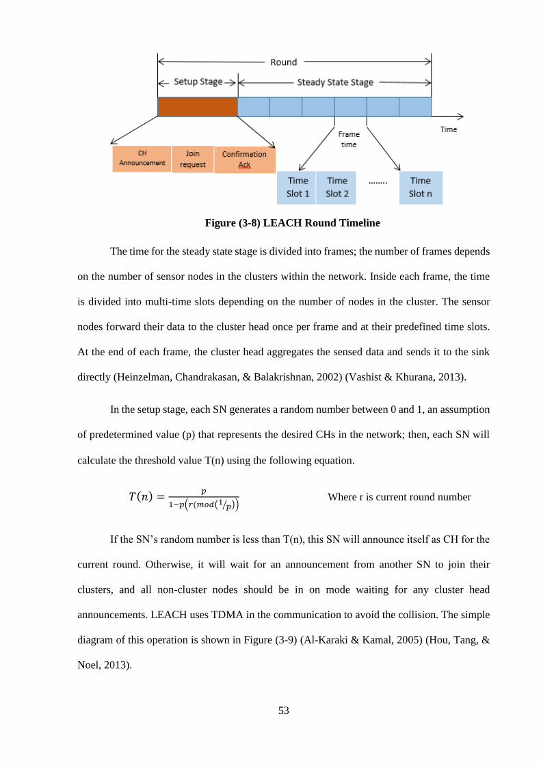
53
The time for the steady state stage is divided into frames; the number of frames depends
on the number of sensor nodes in the clusters within the network. Inside each frame, the time
is divided into multi-time slots depending on the number of nodes in the cluster. The sensor
nodes forward their data to the cluster head once per frame and at their predefined time slots.
At the end of each frame, the cluster head aggregates the sensed data and sends it to the sink
directly (Heinzelman, Chandrakasan, & Balakrishnan, 2002) (Vashist & Khurana, 2013).
In the setup stage, each SN generates a random number between 0 and 1, an assumption
of predetermined value (p) that represents the desired CHs in the network; then, each SN will
calculate the threshold value T(n) using the following equation.
𝑇(𝑛) =𝑝
1−𝑝(𝑟(𝑚𝑜𝑑(1𝑝⁄ ))
Where r is current round number
If the SN’s random number is less than T(n), this SN will announce itself as CH for the
current round. Otherwise, it will wait for an announcement from another SN to join their
clusters, and all non-cluster nodes should be in on mode waiting for any cluster head
announcements. LEACH uses TDMA in the communication to avoid the collision. The simple
diagram of this operation is shown in Figure (3-9) (Al-Karaki & Kamal, 2005) (Hou, Tang, &
Noel, 2013).
Figure (3-8) LEACH Round Timeline

54
Despite LEACH being considered an energy efficient routing protocol compared with
other data-centric protocols, it has many drawbacks, as listed below (Enam, Imam, & Qureshi,
2012; Ramesh & Somasundaram, 2011) (Tong & Tang, 2010):
- The clustering is unbalancing and may not cover all the network area.
- The inefficient cluster head selection scheme is based on probability and random
selection, and does not consider the remaining energy of the sensor nodes. Therefore,
the nodes with low energy level may be selected as a cluster head, and this will lead to
increased power consumption for the nodes.
- The random selection of the CHs makes it difficult to predetermine the CHs to distribute
it uniformly to cover the whole network area.
- The dynamic clustering may cause an overhead on the network, and it does not take into
consideration the SNs position and location.
Regarding communications that take place during the functioning of this protocol,
Figures (3-10) illustrate the number of transmissions and receiving processes in both cases, for
cluster head node and cluster member nodes. It is noticeable that there are a significant number
of communications during the protocol activities and this leads to increasing the amount of
energy consumption and affects the network lifetime. Therefore, this should be controlled and
managed to improve the network lifetime, and this is one of the main thesis contributions.
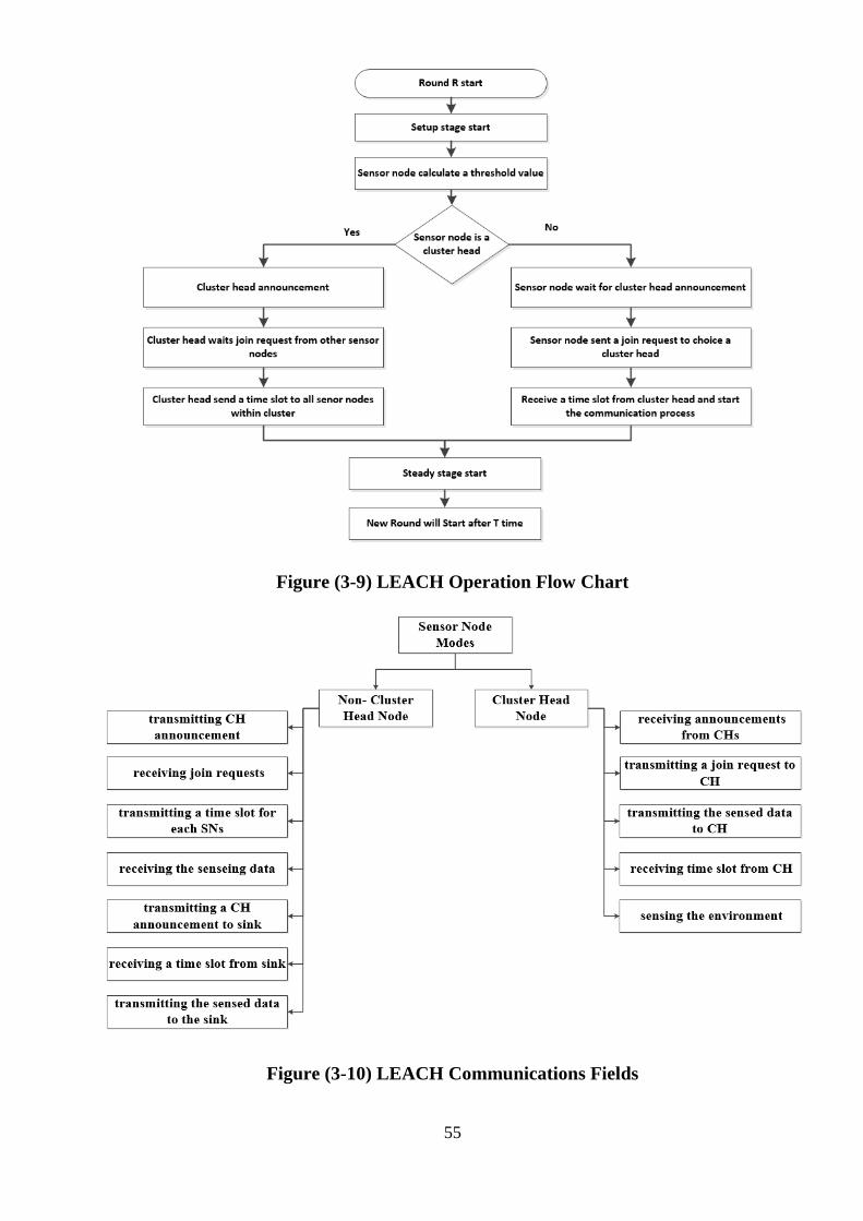
55
Figure (3-9) LEACH Operation Flow Chart
Figure (3-10) LEACH Communications Fields

56
Owing to LEACH’s popularity, there are various studies that have been introduced in
this area. The implementation of this protocol in the real time is introduced in (Hou et al., 2013)
which is the first implementation of LEACH protocol in the real wireless sensor nodes, where
the implementation is based on the TinyOS and Crossbow MICA2 hardware platform, and it is
considered a significant contribution in the field of WSN.
There are various studies and surveys that have been proposed based on the principles
of this. For instance, the authors in (Mahboub, Arioua, & Ez-Zazi, 2016) (Aslam et al., 2013)
(Aslam et al., 2012) (Bhakti Parmar, 2014) (Hani & Ijjeh, 2013) (Kaur & Grover, 2015; Sheth
& Rathod, 2015) (Upadhyay & Swaroop, 2016) introduce surveys and reviews on the different
types of protocols whose functions are based on LEACH.
Most of the available distributed clustering routing protocols are based on the concept
of LEACH protocol and each one of this protocol try to enhance the LEACH protocol and
improving the network lifetime. Some of these protocols will now be discussed in next section.
2- LEACH-Balanced (LEACH-B):
To enhance the cluster head selection process in LEACH, the LEACH-B is proposed in
(Tong & Tang, 2010). In this protocol and during the first round, the cluster head selection
follows the same procedure as in LEACH while the second selection based on node's remaining
energy. The selection technique makes the number of cluster heads near the optimum and thus
will lead to balancing the energy consumption; the result shows that this protocol is better than
LEACH in terms of energy consumption, and it maximises network lifetime, but at the same
time it increases network overhead during the cluster head selection.
57
3- Extended-LEACH (E-LEACH)
Extended -LEACH (Xiangning & Yulin, 2007) improves the cluster head selection
scheme of LEACH. The decision of cluster head selection based on nodes energy level. As in
LEACH, the protocol operation is divided into rounds, for the initial round, all the nodes have
the probability of being a CH, so its random process. While in the following rounds, the nodes
with high energy level will be a cluster head for the current round. The results show that the
network lifetime in the E-LEACH is longer than LEACH.
4- Energy-Efficient LEACH (EE-LEACH)
To improve the network lifetime, a Gaussian distribution model was used in EE-
LEACH (Arumugam & Ponnuchamy, 2015) for better coverage in the sensing area. The cluster
formation and cluster head selection are based on nodes energy level. The results illustrate that
the EE-Protocol is better than LEACH in terms of energy consumption reduction and packet
delivery ration. This work focused on how to reduce the energy consumption, but it had lacked
in the security issues and attacks.
5- Energy Efficient Extended LEACH (EEE-LEACH):
As mentioned previously, the communication in LEACH protocol is single hop.
Therefore, to minimise the distance between the nodes in order to minimise the energy
consumption, the EEE-LEACH clustering protocol is introduced in (Pare & Dongre, 2015).
This protocol based on multi-level communication and a new master node are selected to
cooperate with the main cluster head during data processing. The results show the new protocol
is more efficient than LEACH and the network lifetime had been improved.

58
6- Power-Efficient Gathering Sensor Information Systems (PEGASIS):
The concept of the protocol is based on chain clustering (Lindsey & Raghavendra,
2002), a chain of nodes formed from the nodes to the sink. The chain formation is based on a
greedy algorithm. To reduce the overhead that occurs in the clustering function, but it adds a
new overhead related to chain shaping. The results show that network lifetime and performance
under PEGASIS is better than the LEACH.
7- PEGASIS-LEACH:
To improve the PEGASIS and LEACH protocols, an optimum cluster-based chain
protocol proposed in (Razaque, Abdulgader, Joshi, Amsaad, & Chauhan, 2016). This protocol
is gathering the fundamentals of the LEACH and PEGASIS to improve the energy efficiency.
In other words, its combine the chain formation scheme with the clusters in data forwarding.
The results shows that the new protocol outcome the LEACH and PEGASIS in terms of energy
consumption, the number of dead nodes and network lifetime.
8- Threshold sensitive Energy Efficient Sensor Network Protocol (TEEN):
To improve the performance of the LEACH to work in criticial application, an energy
efficiency routing protocol for reactive networks known as TEEN (Threshold sensitive Energy
Efficient Sensor Network Protocol) is introduced in (Manjeshwar & Agrawal, 2001). TEEN
protocol can be used in a reactive network where the nodes react immediately to any changes
in the sensing environmet. Therefore, this protocol is suitable to work in time critical
applciations.
In this protocol, two thresholds sensed attribute, hard and soft threshold, are used to
enable the SNs to sense the critical conditions and prevent them from sensing the data
continuously, which will reduce the energy consumption. The main drawback in this protocol
59
is that if the threshold values do not reach the SNs, they will stop communication and sensing
and will not be used in periodic applications.
9- Adaptive Periodic-TEEN (APTEEN):
Because of the TEEN protocol is suitable for the reactive network only, an extension of
the TEEN protocol APTEEN (Adaptive Periodic-TEEN) is proposed (Manjeshwar & Agrawal,
2002) to be used in both proactive and reactive mode networks (Hybrid networks). The nodes
participating in the transmission are only the nodes with sensed data at or below the threshold
value. Its main drawback is in TEEN, which is the extra overhead, and the complexity of
clustering function in multi-level.
10- LEACH-Selective Cluster (LEACH-SC):
In order to improve the cluster head selection process in LEACH, (Iqbal et al.; Jun, Xin,
Junyuan, & Zhengkun, 2010) propose a routing protocol known as LEACH-SC (LEACH-
selective cluster). This protocol is considered to be a distance-based clustering protocol, and
the author assumes that the SNs know their locations and positions. A new scheme is used
during cluster head selection to achieve energy efficiency. The SNs join the CH that is nearest
to the middle point in the distance between the SN itself and the sink. In the results, this protocol
outperforms the LEACH protocol in terms of energy consumption and prolonged network
lifetime.
11- Narrative-LEACH (N- LEACH):
To optimise the nodes energy level and improve the Intra and inter communication of
LEACH, a clustering protocol based on LEACH called narrative-LEACH is proposed in

60
(Tiwari, 2016). This protocol uses the multi hop scheme to optimise the energy of the network.
The cluster head selection in this protocol is based on a tree where any node that is in the tree
can reach the sink while there is nothing like this in LEACH. The results show that the new
protocol is the outcome of the LEACH protocol and improves the network lifetime. In spite
there is an improvement in the lifetime, but the drawback of is protocol is in using the multi
hope communication that causes an extra overhead on the nodes near the sink.
12- Two Level LEACH (TL-LEACH):
As described in LEACH which is suitable for low density networks, and in order to
improve this, a random and distributed protocol is proposed in (Loscri, Morabito, & Marano,
2005). The protocol operation based on the two-level hierarchy to allow for better energy
consumption especially in high density networks. The role of the primary and secondary cluster
heads is rotated randomly. The results show that the new protocol is better than LEACH and
the network lifetime had been improved by 30% than in LEACH.
13- Double Cluster Based Energy Efficient Routing Protocol:
In WSN, the most important aim is to prolong network lifetime. According to this, a
routing protocol known DL-LEACH which based on LEACH is proposed in (Li & Liu, 2016).
This protocol improved the cluster head selection of LEACH. In LEACH, the CH selection is
random while in DL-LEACH, the selection of the cluster head depends on the nodes energy
level and the distance between the nodes in order to make the selection more reasonable and
balane the energy consumption among the nodes. The CH selection had two levels, the first
level is where the data is received, while the second level is responsible for forwarding the data

61
to the sink. According to the results, the protocol improves the network lifetime by 75% more
than the LEACH.
14- Cognitive LEACH:
There are various researches in order to improve the LEACH protocl. All the avaiables
reseraches enhanced either the cluster head selection or cluster formation schems. One of thes
research is the protocol known as Cognitive Improved LEACH that proposed in (Rahman,
Miah, & Sharmin, 2016). In this protocol, the author changes the cluster head selection, which
is based on the ratio of the nodes’ current residual energy and an initial energy and multiplies
by the root square of nodes’ neighbours. The protocol is evaluated with LEACH in two level
homogeneity networks, and the results show that the new protocol improves the performance
of the network and increases its lifetime.
15- Solar LEACH (S-LEACH):
As the sensor nodes are battery powered, energy saving is considered the most important
factor to keep the network working. To utilities from the renewable energy sources such as the
solar energy supply, a protocol known as LEACH (Solar LEACH) is proposed (Voigt, Dunkels,
Alonso, Ritter, & Schiller, 2004). This protocol is based on the concept of LEACH and the solar
system. The aim of this protocol is to make the cluster head selection process based on the node
with high solar power. The simulation result shows that this new protocol had a significant
impact on the network behaviour and increased the network lifetime.
16- Hybrid Energy-Efficient Distributed clustering (HEED):
By changing the cluster head selection process of the LEACH, a protocol known as
Hybrid Energy-Efficient Distributed clustering (HEED) is proposed in (Younis & Fahmy,

62
2004). The CH selection is based on the nodes energy and the intra-communication cost as well
as multi hop communication. The result shows that the network lifetime had been improved
with the operation of the new protocol. The clustering performing in each round is the same as
in LEACH, and this will cause extra energy consumption and affect the network lifetime. Also,
because it uses multi-hop communication, this will cause the death of the nodes early, especially
near the sink because of the heavy load that they perform.
17- Unequal Cluster-based Routing protocol (UCR):
As mentioned previously, in multi hop clustering, the nodes close to the sink will drain
its energy faster than other nodes, therefore, to minimise the effect of this problem and improve
the performance of HEED protocol, (Chen et al., 2007) proposed an Unequal Cluster-based
Routing (UCR) protocol. The protocol form the clusters with different sizes based on the
distance to the sink. The size of the cluster whose cluster head node is closer to the sink will be
smaller than the other that is further away from the sink. The simulation shows that there is an
improvement in terms of network lifetime more than HEED.
18- Centralised Energy Efficient Distance (CEED):
A Centralized Energy Efficient Distance (CEED) routing protocol is proposed in
(Gawade & Nalbalwar, 2016). In this protocol, the nodes deployment is random, and the cluster
head selection is optimised based on the probability process, also the protocol based on multiple
systems where only the cluster head nodes near the sink can forward the data. The results show
that the protocol improves the system and more so than other routing protocols such as LEACH.

63
19- Unequal Clustering Routing for Mobile Education Protocol:
To utilities from the clustering protocol in learning and education applications, a novel
energy balancing unequal routing protocol for mobile education (mobile learning) proposed in
(Zhang, Liu, Zhang, & Liang, 2017). The clusters formed based on a circle area with the sink
as the centre. These circles area had a various radius in order to balance the energy consumption.
Simulation results show that the network lifetime had been prolonged and the energy
consumption of the nodes had been balanced.
20- Double-phase Cluster-head Election Clustering Protocol (DEC):
Heterogeneity of the nodes should be taken into consideration during the designing of
clustering protocol. Therefore, a novel distributed clustering protocol had been proposed. The
cluster head selection based on a double phase selection scheme. The selection process had two
steps, in the first step, a temporary cluster head will be selected based on its initial energy and
current energy level. While in the second step, a new node with high energy level among the
cluster members will be selected as a new cluster head and replace the old one. This scheme
enables the nodes with more energy level to be a cluster head. The results show that the new
protocol had better stability than the existing heterogeneous clustering protocol.
21- Energy potential-LEACH (EP-LEACH)
EP-LEACH (Xiao, Zhang, & Dong, 2013) based on EH-WSN (Energy Harvesting
WSN) to improve the network lifetime of LEACH protocol. In EH-WSN, the nodes have the
ability to harvest their power from the environment and have a rechargeable battery. The
process of EP-LEACH is same as LEACH with two different modifications. For the first
modification, the node that has more energy harvest level have a high change to be a cluster
64
head. Accordingly, the nodes can become a CHs with an ultimate number of times. The results
showed that the EP-LEACH is better than LEACH in terms of network lifetime, but it has poor
performance in terms of complexity and message overhead.
3-4-2 Centralised Clustering based Routing Protocols:
The advantage of the centralised clustering that uses the network topology information
in order to form good clusters in the network to minimise the amount of energy consumption
during the clustering function. The protocols based on the centralised classification that is
location-ware where the nodes know their location and are used during the clustering function.
The clustering function and all necessary information are performed by central nodes, in
general, is the sink, and all the available protocols use the sink as the controller node. The nodes
should send their information at the beginning of each round to the sink to start the clustering
function but the main difference with our contribution is in this step, where the server is
responsible for network management, and the nodes need to send their information at the
beginning of the initial round only. After sending their information, there are no
communications between the nodes during the cluster formation. The general flowchart for this
category and all available clustering routing protocols are flow same steps is shown in Figure
(3-11).
A survey of available centralised protocols is introduced in (Zanjireh & Larijani, 2015),
where the authors aimed to introduce a full taxonomy of available centralised protocols in
WSN. The available centralised clustering protocols are as follows:

65
Figure (3-11) Centralised Clustering Protocol Flowchart
1. Centralized LEACH (LEACH-C):
The first centralised protocol is (Centralized Low Energy Adaptive Clustering
Hierarchy) (Heinzelman et al., 2002), and the aim of this protocol is to produce better clustering
than LEACH. The sink is responsible for the clustering process, and the steady state is the same
as in LEACH. The sensor nodes should know their position while the sink clusters the nodes
based on specific energy level cluster heads from the nodes that have energy above the average
energy level. The sink produces a table with the nodes that are efficient enough to be cluster
heads and sends it to the network. The sink uses an optimisation algorithm to determine the
optimum number of clusters, and the table of cluster head nodes will be fixed. The operation
steps for this protocol is as shown in Figure (3-12).

66
The LEACH-C protocol shows improvement of 40% more than LEACH regarding
network performance. The main drawback is sending information process at the start of each
round. This step consumes additional energy for all nodes; will increase the overhead energy
consumption regarding communications. Furthermore, the list of CHs nodes is unchangeable
that lead to unbalancing the CH selection among the whole nodes in the network.
Figure (3-12) LEACH-C Operation Flow Chart

67
2. Modified LEACH-C:
In order to improve the cluster head selection process in LEACH-C, A modified
LEACH-C protocol is proposed in (Parmar & Thakkar, 2016), and this protocol uses the
distance between the CHs and cluster members as well as the distance between cluster members
and the sink as the main parameter. According to the simulation, the results explain that this
new protocol improves the network lifetime and it is better than the LEACH-C protocol.
3. LEACH Central Constrained (LEACH-CC):
To balance the energy consumption for the nodes and improve the cluster head selection
in LEACH-C and modified LEACH-C, a develpoed protocl was introduced in (Parmar &
Thakkar, 2016). The change was in the process of cluster head selection by changing the range
of the nodes that will be cluster heads to be based on their energy level. The simulation results
show an improvement of the network performance with LEACH-CC than LEACH-C in term if
network lifetime.
4. Energy Efficient LEACH-C (EELEACH-C):
To enhance the network lifetime and minimise energy consumption, a version of
LEACH-C is proposed in (Parmar & Thakkar, 2016), using an energy efficient LEACH-C
protocol for wireless sensor network. The cluster head selection is based on a sort of algorithm
operated by the sink, and the sink creates a list of nodes sorting in descending order based on
their energy level. The node with maximum energy level will be a cluster head for the current
round. Whilst there is an improvement in the network with this protocol, the main drawback is
if there are two nodes with the same energy level, the node that will be a cluster head is based
on nodes id, which is not an efficient method.

68
5. Base-Station Controlled Dynamic Clustering Protocol (BCDCP):
Another centralised clustering protocol is introduced in (Muruganathan, Ma, Bhasin, &
Fapojuwo, 2005 ). The operation of the protocol is based on the communication among the
cluster head based on multi-hop where the CHs send their data to other CHs until it reaches the
sink. The CH selection is based on a random process using cluster splitting algorithm that
divides the network into two main clusters and proceeds by dividing the sub-clusters into
smaller clusters until the desired number of clusters is achieved. The number of nodes within
the clusters are the same. The performance of this protocol shows that the energy consumption
is minimised comparing with LEACH and LEACH-C and the network lifetime is improved.
6. Centralised Genetic-Based Clustering (CGC):
To optimise the number of cluster head in the network, a centralised genetic-based
clustering protocol for WSN is proposed in (Hatamian, Barati, Movaghar, & Naghizadeh,
2016). In this protocol, the genetic algorithm is used to find the optimum number of cluster
heads. The networks are clusters based on a new technique known as onion approach, where
the network is divided into several layers to reduce the communications among the cluster head
nodes. The results show that the network performance and the lifetime are increased and the
packet delivery is significantly improved.
7. Centralised Balance Clustering Routing Protocol:
To make the clustering balanced in the whole network lifetime and suitable with non-
uniform distributed nodes, a clustering routing protocol based on a centralised approach is
proposed in (Chen, Li, & Kuo, 2013). The aim of this protocol is to balance the clustering
through the network operations and this done by designing a systemic clustering algorithm. The

69
clustering formed in a hexagonal shape, and the selection of the cluster head node based on
energy and distribution of nodes. The simulation results show that the new protocol improves
the network lifetime than LEACH.
To define various points of difference among the available clustering routing protocols,
Table (3-1) summaries and review the main points in both distributed and centralised clustering
protocols.
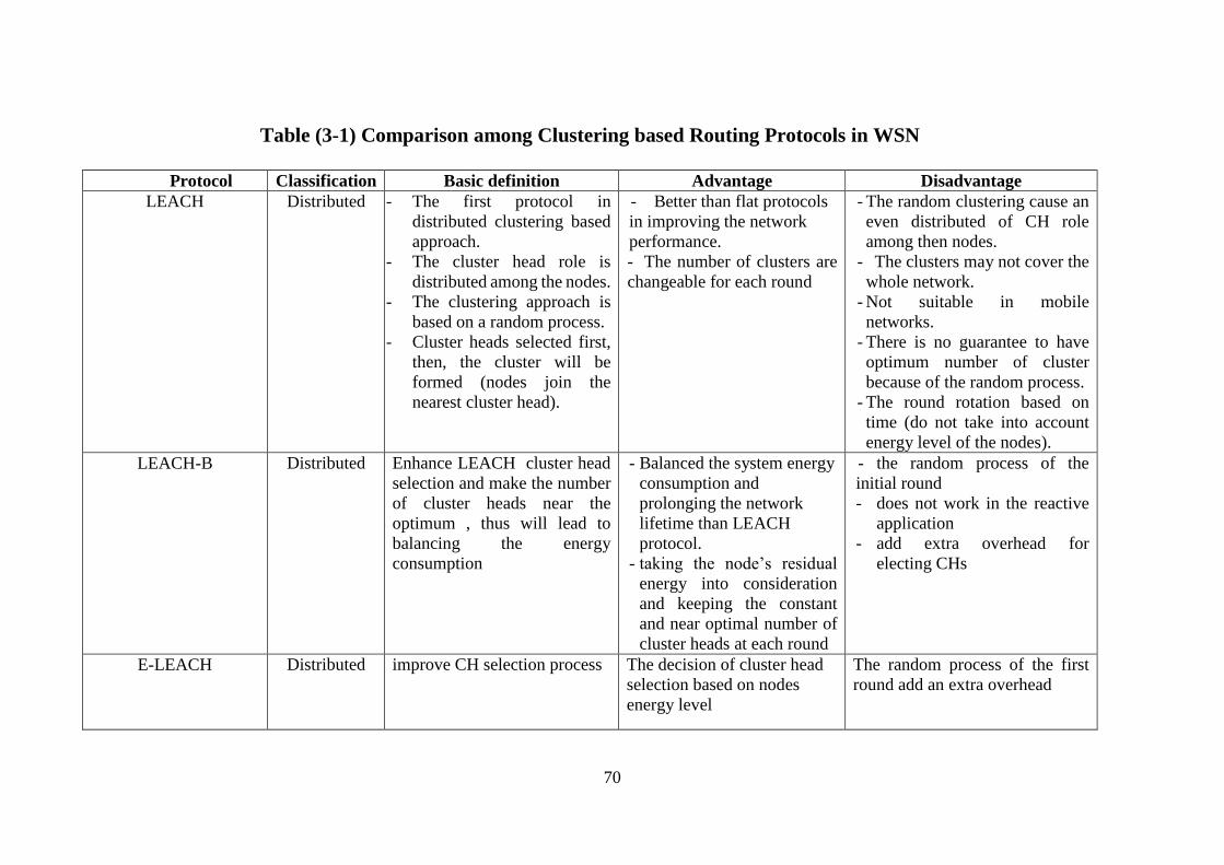
70
Table (3-1) Comparison among Clustering based Routing Protocols in WSN
Protocol Classification Basic definition Advantage Disadvantage
LEACH Distributed - The first protocol in
distributed clustering based
approach.
- The cluster head role is
distributed among the nodes.
- The clustering approach is
based on a random process.
- Cluster heads selected first,
then, the cluster will be
formed (nodes join the
nearest cluster head).
- Better than flat protocols
in improving the network
performance.
- The number of clusters are
changeable for each round
- The random clustering cause an
even distributed of CH role
among then nodes.
- The clusters may not cover the
whole network.
- Not suitable in mobile
networks.
- There is no guarantee to have
optimum number of cluster
because of the random process.
- The round rotation based on
time (do not take into account
energy level of the nodes).
LEACH-B
Distributed Enhance LEACH cluster head
selection and make the number
of cluster heads near the
optimum , thus will lead to
balancing the energy
consumption
- Balanced the system energy
consumption and
prolonging the network
lifetime than LEACH
protocol.
- taking the node’s residual
energy into consideration
and keeping the constant
and near optimal number of
cluster heads at each round
- the random process of the
initial round
- does not work in the reactive
application
- add extra overhead for
electing CHs
E-LEACH
Distributed improve CH selection process The decision of cluster head
selection based on nodes
energy level
The random process of the first
round add an extra overhead

71
EE- LEACH Distributed The formation of the clusters
and cluster head selection is
based on nodes energy level
Use Gaussian for better node
coverage
Lacks of security
EEE-LEACH
Distributed Based on multi-hops
communications to reduces the
distance from cluster head to
base station
introduces Master Cluster
Heads along with Cluster
Heads to balance the CHs
role
- The probability of select the
master CH is effected the protocol
performance and should be the
optimum value
- Location unaware
- Random CH selection
PEGASIS Distributed Based on chain clustering To reduce the overhead that
occurs in the clustering
function and data gathering
- adds a new overhead related to
chain shaping
- lacks dynamicity
PEGASIS-LEACH Distributed Gathering the fundamentals of
the LEACH and PEGASIS to
improve the energy efficiency
Prolongs the network lifetime
and improve dynamicity
- Location unaware
-Not suitable for heterogeneous
network
TEEN Distributed two thresholds sensed attribute,
hard and soft threshold, are
used to enable the SNs to sense
the critical conditions and
prevent them from sensing the
data continuously, which will
reduce the energy
consumption.
- Work in critical
applications
- Suitable for event based
applications and real time
applications
- provides a trade-off
between the accuracy and
energy consumption
- the threshold values do not reach
the SNs, they will stop
communication and sensing and
will not be used in periodic
applications.
- Unsuitable for regular data
gathering applications.
- Work in reactive applications.
APTEEN Distributed Combines the charactersitics
of both proactive and reactive
networks to provide periodic
data collection.
Use in Hybrid networks Its main drawback is in TEEN,
which is the extra overhead, and
the complexity of clustering
function in multi-level.
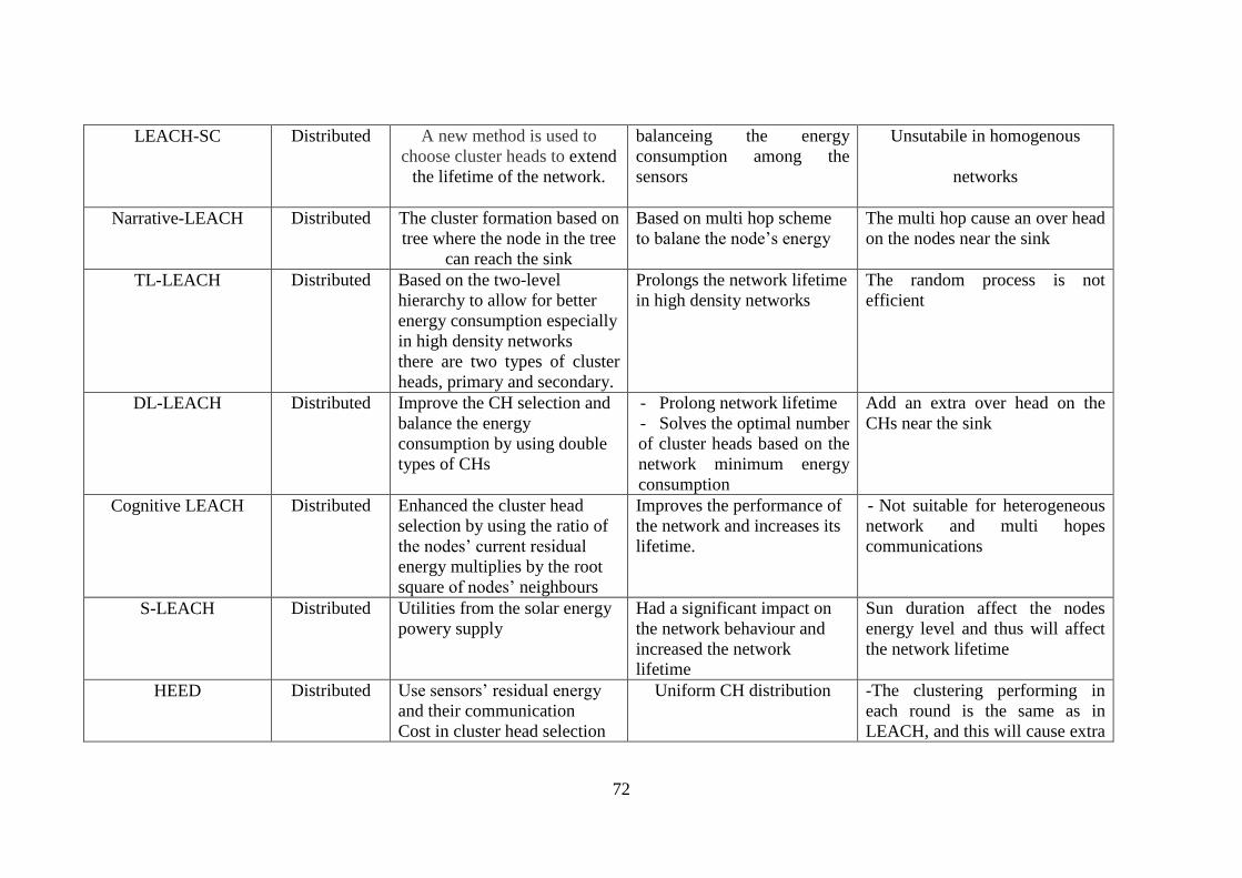
72
LEACH-SC Distributed A new method is used to
choose cluster heads to extend
the lifetime of the network.
balanceing the energy
consumption among the
sensors
Unsutabile in homogenous
networks
Narrative-LEACH Distributed The cluster formation based on
tree where the node in the tree
can reach the sink
Based on multi hop scheme
to balane the node’s energy
The multi hop cause an over head
on the nodes near the sink
TL-LEACH
Distributed Based on the two-level
hierarchy to allow for better
energy consumption especially
in high density networks
there are two types of cluster
heads, primary and secondary.
Prolongs the network lifetime
in high density networks
The random process is not
efficient
DL-LEACH Distributed Improve the CH selection and
balance the energy
consumption by using double
types of CHs
- Prolong network lifetime
- Solves the optimal number
of cluster heads based on the
network minimum energy
consumption
Add an extra over head on the
CHs near the sink
Cognitive LEACH Distributed Enhanced the cluster head
selection by using the ratio of
the nodes’ current residual
energy multiplies by the root
square of nodes’ neighbours
Improves the performance of
the network and increases its
lifetime.
- Not suitable for heterogeneous
network and multi hopes
communications
S-LEACH Distributed Utilities from the solar energy
powery supply
Had a significant impact on
the network behaviour and
increased the network
lifetime
Sun duration affect the nodes
energy level and thus will affect
the network lifetime
HEED Distributed Use sensors’ residual energy
and their communication
Cost in cluster head selection
Uniform CH distribution -The clustering performing in
each round is the same as in
LEACH, and this will cause extra

73
energy consumption and affect
the network lifetime
- Multi-hop communication, this
will cause the death of the nodes
early
UCR Distributed Forms the clsuters with
different clsuter size where the
CH near the sink will have
smaller size than the CH
faraway from the sink
Improve the network lifetime
in multi hope networks
Low robustness
CEED Distributed - Cluster head selection is
optimised based on the
probability process
- Protocol based on multiple
systems where only the
cluster head nodes near the
sink can forward the data
Improves the network
lifetime and stability period
The problem of multi hope
communications
Unequal Clustering
Routing for Mobile
Education Protocol
Distributed The clusters formed based on a
circle area with the sink as the
centre. These circles area had a
various radius in order to
balance the energy
consumption
- To utilities from the
clustering protocol in learning
applications
-Reduces the energy
consumption of cluster
reconstruction
-Not suitable if the sink locates
outside the sensing area.
-Not suitable for heterogeneous
networks
DEC
Distributed The cluster head selection
based on a double phase
selection scheme
Use in heterogeneous
networks
Add extra over head in CH
selection
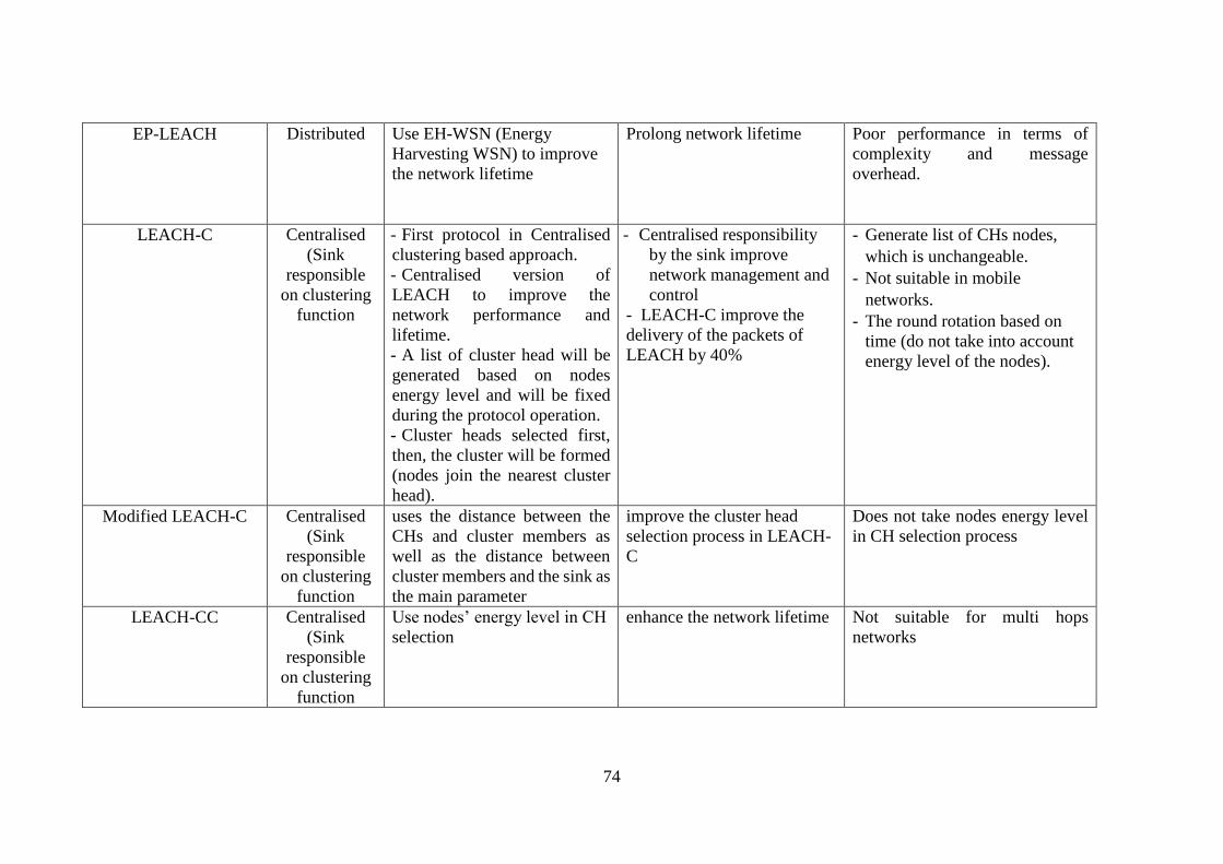
74
EP-LEACH
Distributed Use EH-WSN (Energy
Harvesting WSN) to improve
the network lifetime
Prolong network lifetime Poor performance in terms of
complexity and message
overhead.
LEACH-C Centralised
(Sink
responsible
on clustering
function
- First protocol in Centralised
clustering based approach.
- Centralised version of
LEACH to improve the
network performance and
lifetime.
- A list of cluster head will be
generated based on nodes
energy level and will be fixed
during the protocol operation.
- Cluster heads selected first,
then, the cluster will be formed
(nodes join the nearest cluster
head).
- Centralised responsibility
by the sink improve
network management and
control
- LEACH-C improve the
delivery of the packets of
LEACH by 40%
- Generate list of CHs nodes,
which is unchangeable.
- Not suitable in mobile
networks.
- The round rotation based on
time (do not take into account
energy level of the nodes).
Modified LEACH-C Centralised
(Sink
responsible
on clustering
function
uses the distance between the
CHs and cluster members as
well as the distance between
cluster members and the sink as
the main parameter
improve the cluster head
selection process in LEACH-
C
Does not take nodes energy level
in CH selection process
LEACH-CC Centralised
(Sink
responsible
on clustering
function
Use nodes’ energy level in CH
selection
enhance the network lifetime Not suitable for multi hops
networks

75
EELEACH-C Centralised
(Sink
responsible
on clustering
function
Use sort algorithm in CH
selection to create the CH list
and the node with high energy
level will be CH for the current
round
Prolong network lifetime if there are two nodes with the
same energy level, the node that
will be a cluster head is based on
nodes id, which is not an efficient
method
BCDCP Centralised
(Sink
responsible
on clustering
function
Based on multi-level CH-to-
CH communications and has
equal size of clusters
Extend the network lifetime - The selection of multi CH is
randomly
- Adding one CH o forward data
to sink cause an extra over head
on this CH
CGC Centralised
(Sink
responsible
on clustering
function
To optimise the number of
cluster head in the network
- Suitable for large-scale
network because of using
an onion approaches
- Improve network lifetime
Not suitable for heterogeneous
and multi hope networks
Centralised Balance
Clustering Routing
Protocol
Centralised
(Sink
responsible
on clustering
function
Form the clusters in hexagonal
shapes and optimise the cluster
head selection
Balancing the energy
consumption of the nodes
Prolong network lifetime
Improve the data transmit
effectively
Lacks of scalability
Number of nodes in each cluster
is the same

76
3-5 Critical Analysis
As shown from the previous clustering routing protocols in WSN, all the available
researches focused on changing either the approach of cluster formation or cluster head
selection as a new technique to improve the network lifetime. However, in terms of number of
communications, the same procedures had been followed for all available protocols.
The review for the available protocols help to find the appropriate assumptions and
properties that can used in the new design in order proposed better protocol and achieve the aim
of the research. Therefore, a new centralised and virtualised clustering routing (VCR) protocol
had been proposed. The main concept of the new protocol is to minimise the number and
amount of communications during the clustering function in both distributed and centralised
protocols as well as using efficient techniques in cluster formation, cluster head selection, rotate
CH role and cluster re-formations in order to improve network lifetime.
According to this, the general flowchart of the new protocol will be different from
distributed and centralised types and it shown in Figure (3-13). The next chapter will introduce
the main characteristics and functions for the VCR protocol.
3-6 Summary
In this section, the clustering functions and cluster-based protocol classifications have
been reviewed and explained. The most popular type is the distributed where the nodes are
responsible for the clustering function. The main problem, which should be managed in
distributed clustering protocols, is the communications during the cluster formation and cluster
head selection. The first distributed clustering protocol (LEACH), which is the case study of
this thesis, as well as various examples of the available distributed clustering based routing
protocols, have been discussed and reviewed.

77
Furthermore, the other protocol type is the centralised protocol. The most important
problem in this type is the process of information sending at the beginning of each round to
provide the sink with their information.
Figure (3-13) Proposed Protocol (VCR) operation flow chart

78
Chapter Four
The Virtualised Clustering Routing (VCR) Protocol
4-1 Introduction
In this chapter, the principles, functions, and characteristics of the proposed protocol
are discussed.
As discussed earlier, the communications (sending and receiving) among the sensor
nodes and between them and the sink are the main source of energy dissipation during the
operation of clustering function; therefore, to achieve better energy efficiency, these
communication activities need to be controlled and minimised. For these reasons, a new
virtualised clustering protocol is proposed in this chapter.
4-2 The Assumptions of the VCR Protocol:
In the clustering based routing protocols, the most important issues are how the clusters
are formed and which node will be the cluster head to improve the energy efficiency and
maximise network lifetime.
In light of this, the following list presents the proprieties and the assumptions that are
used during the design of the proposed protocol in order to achieve the design aim and improve
network lifetime; Figure (4-1) outlines these features:
79
Dynamic cluster formation and cluster head selection: which mean as soon as the
clusters formed and/or cluster head selected, they will be not fixed and their rotation
will based on certain conditions that will be discussed in details in this chapter.
Homogenous: all the sensor nodes have the same energy level (at the beginning of the
process), processing and storage capabilities. This was selected to balance the roles
among all nodes.
Centralised/Virtualised: the NFV server will be responsible for the majority of the
computational activities.
Non-probabilistic: a more deterministic technique will be used to select the cluster head
and form the clusters to achieve energy efficiency and improve network lifetime.
The sensor nodes have a fixed position after deployment (stationary).
The sink is in a stationary mode and does not have energy constraints.
For research purposes, the sink will be initialised with the size of the network (number
of nodes in the network).
The sensor nodes will always have data to send within their time slot.
Inter and intra-communication will be a single hop.
The sensor nodes know their IDs, location and initial energy, as well as sink ID and
position, and use them during the initial stage.
The energy consumption of sleep mode is small and has a negligible effect on the
overall consumption (Han, Zhang, & Yang, 2008; Liu, Tsui, & Zhang, 2010;
Srivastava, 2002).
The new selection of the cluster head for each cluster can be restarted based on an
energy threshold value. When the energy of CH comes down below this value, the NFV
server will re-select new a CH (the remaining energy of CH can be found by subtracting
its initial energy level from the consumed value).

80
Clusters will be formed first, and then the cluster head selection for each cluster will be
selected based on a certain cost function.
The re-clustering process (reform the clusters) will restart when all nodes within the
clusters have been selected as cluster head in previous rounds.
The intra-communications between the CHs and the base station (BS) use a unique code
to prevent any packet loss between the CHs and the BS.
The inter communications between the sensor nodes and their cluster heads are based
on Time Division Multiple Access (TDMA) technique that sets a time slot for each
node for sensing their data.
Figure (4-1) Virtual Clustering Routing (VCR) Protocol Proprieties

81
4-3 VCR Protocol Functions:
The general operation of the VCR protocol divided into various functions as follows,
the more details for each function will be explained in the following next sections:
1- Node discovery function: this is the initial stage where the nodes send their information
(node ids, energy level and position) to the server via the sink. For research purposes, the
sink will be initialised with the size of the network (number of nodes in the network).
2- Calculation Function: After receiving the nodes’ information by the server, various
calculation process will be done in order to start the clustering function.
3- Clustering function: the clustering step splits into two main stages, setup and steady
state. The setup stage contains the cluster formation and cluster head selection
functions. The server will manage and control these functions based on certain
parameters and will send the result to the nodes. On the other hand, the sensor nodes,
after receiving the clustering decision, will start to transmit the sensed data to their
cluster head node, which constitutes the steady stage step. To understand the timescale
of the cycle, Figure (4-2) represents the timescale for the cycles during the protocol
operation. From this figure, it shows that for the next cycles, the timescale will contain
clustering decision from the NFV server
4- Energy Consumption calculation Function: after completing the clustering function,
the server will estimate the amount of energy consumption using the proposed
mathematical model that will explain in the next chapter, in order to manage the
network operation and checking if the cluster head should be reselected or the cluster
should be reformed.
5- Cluster Head reselection function: this function will be activated when the cluster head
node need to be change.
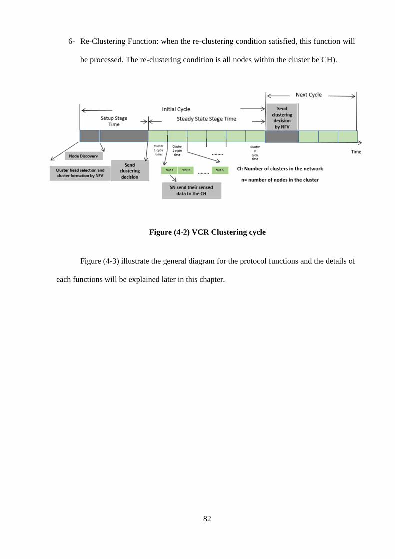
82
6- Re-Clustering Function: when the re-clustering condition satisfied, this function will
be processed. The re-clustering condition is all nodes within the cluster be CH).
Figure (4-2) VCR Clustering cycle
Figure (4-3) illustrate the general diagram for the protocol functions and the details of
each functions will be explained later in this chapter.

83
Figure (4-3) VCR Functions

84
Regarding communications that take place during the operation of the proposed
protocol, Figure (4-4) illustrates the number of transmissions and receiving processes in both
cases.
Figure (4-4) VCR Communications Fields
4-3-1 Node Discovery Function
This is the initial stage where the sensor nodes will send their information to the sink
that will forward it to the server as in Figure (4-5). As mentioned previously, the sink will
initialise with the size of the network (number of nodes in the network).The nodes information
will be sent using node discovery packet (SN_Dis_PDU) that shown in Figure (4-6), full details
of this PDU is in Appendix A. The sending process occurs at the beginning of the initial round
only, and it is not repeated.
The sending process performed just once at the beginning, unlike the existing
centralised clustering protocols where the sending occurs at the start of each round.

85
After that, the sink will forward the infirmation to the server using a Sink to Server
Discovery Packet (Sink_Server_Dis_PDU) illustrated in Figure (4-7), full details of this PDU
is in Appendix A.
Figure (4-5) Node Discovery Function
Figure (4-6) Node Discovery Packet (SN_Dis_PDU)
Figure (4-7) Sink_Server_Discovery Packet (Sink_Server_Dis_PDU)
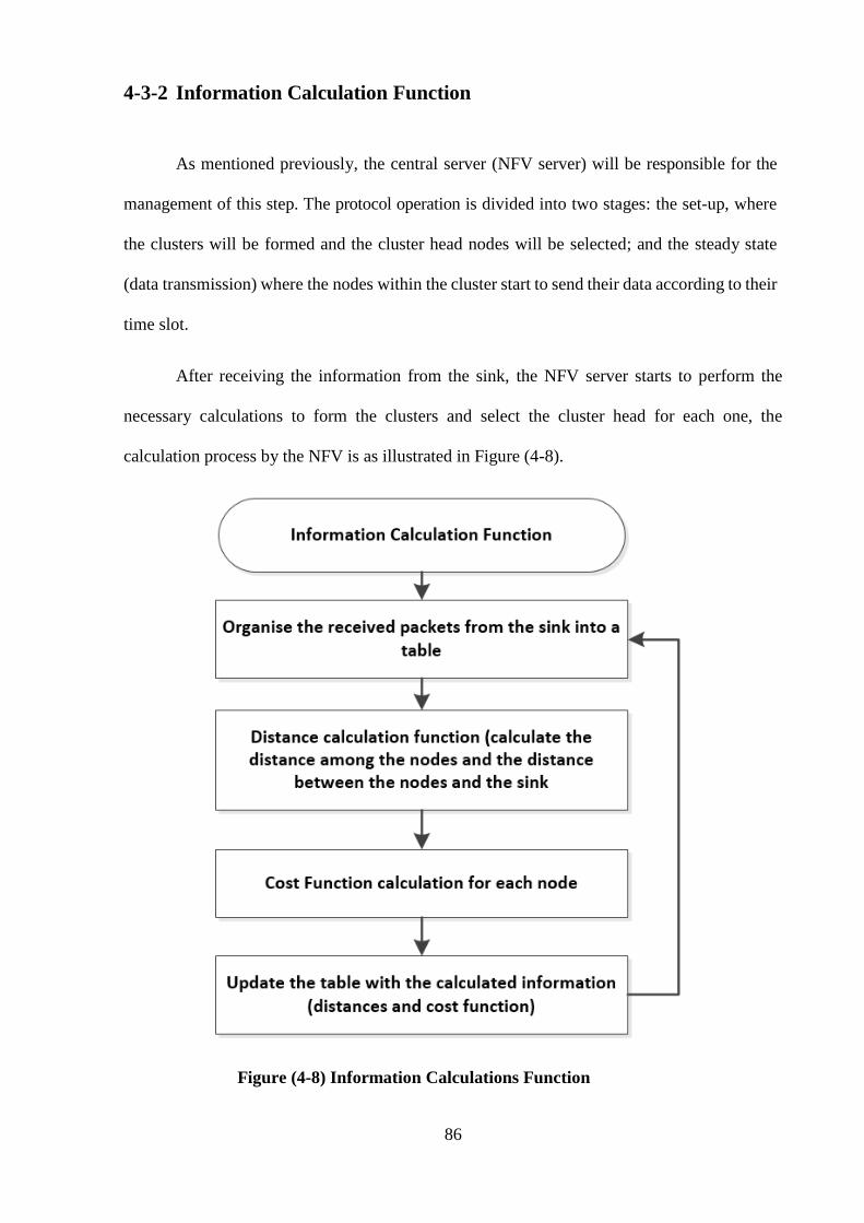
86
4-3-2 Information Calculation Function
As mentioned previously, the central server (NFV server) will be responsible for the
management of this step. The protocol operation is divided into two stages: the set-up, where
the clusters will be formed and the cluster head nodes will be selected; and the steady state
(data transmission) where the nodes within the cluster start to send their data according to their
time slot.
After receiving the information from the sink, the NFV server starts to perform the
necessary calculations to form the clusters and select the cluster head for each one, the
calculation process by the NFV is as illustrated in Figure (4-8).
Figure (4-8) Information Calculations Function

87
The calculation results will be collected in an information table that contents:
1- Node ID
2- Node Position (X and Y coordination)
3- Node’s Current Energy Level
4- Node’s distance to sink
5- Node’s cost function
As mentioned previously, the first calculation process for the server is to calculate the
distance between the nodes and the sink and among the nodes themselves and here the
Euclidian distance will be used to calculate the distance.
The distance formula between the sensor nodes and the sink is as shown in Equation
(4-1). The pseudocode for this step is as in Code (4-1). Then, the server will update the
information table with the result from this step.
Dsn_sink=√(𝒙𝒔𝒊𝒏𝒌 − 𝒙𝒔𝒏)𝟐 + (𝒚𝒔𝒊𝒏𝒌 − 𝒚𝒔𝒏)𝟐
(4-1)
Where (xsink,ysink, xsn, ysn) represents the sink and sensor nodes coordination.
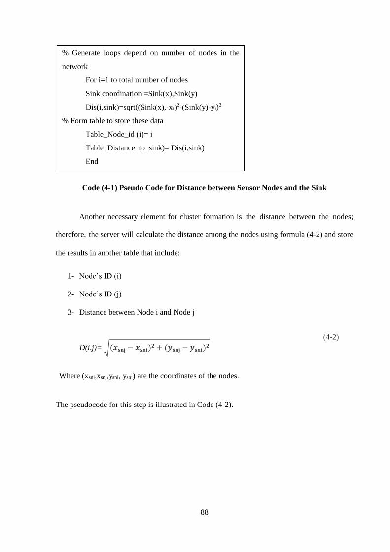
88
Code (4-1) Pseudo Code for Distance between Sensor Nodes and the Sink
Another necessary element for cluster formation is the distance between the nodes;
therefore, the server will calculate the distance among the nodes using formula (4-2) and store
the results in another table that include:
1- Node’s ID (i)
2- Node’s ID (j)
3- Distance between Node i and Node j
D(i,j)= √(𝒙𝐬𝐧𝐣 − 𝒙𝐬𝐧𝐢)𝟐 + (𝒚𝐬𝐧𝐣 − 𝒚𝐬𝐧𝐢)𝟐
(4-2)
Where (xsni,xsnj,ysni, ysnj) are the coordinates of the nodes.
The pseudocode for this step is illustrated in Code (4-2).
% Generate loops depend on number of nodes in the
network
For i=1 to total number of nodes
Sink coordination =Sink(x),Sink(y)
Dis(i,sink)=sqrt((Sink(x),-xi)2-(Sink(y)-yi)
2
% Form table to store these data
Table_Node_id (i)= i
Table_Distance_to_sink)= Dis(i,sink)
End

89
For i=1 to total number of nodes
Esn=sensor nodes’ initial energy level
Cost(i)=dis(i,sink)/Esn(i)
Table_nodeid=i
Table_SN_Position=Xsn(i) , Ysn(i)
Table_energy=Esn(i)
Table_distancetosink= Dis(i,sink);
Table.cost= Cost(i);
Code (4-2) Distance between sensor nodes pseudo code
After this step, the server will update the information table with these new data as
described in Pseudocode Code (4-3).
Code (4-3) Pseudo Code for Cost Function Calculation
% Generate loops to find distance between each node
For i=1 to total number of nodes
For j=1 to total number of nodes
Dis(i,j)=sqrt((xj-xi)2-(yj-y1)
2
% Form table to store these data
Table_Node id (i)= i
Table_Node id (j)=j
Table_Distance (i,j)=Dis(i,j)
End
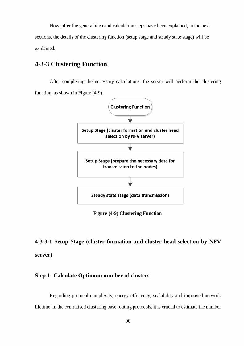
90
Now, after the general idea and calculation steps have been explained, in the next
sections, the details of the clustering function (setup stage and steady state stage) will be
explained.
4-3-3 Clustering Function
After completing the necessary calculations, the server will perform the clustering
function, as shown in Figure (4-9).
Figure (4-9) Clustering Function
4-3-3-1 Setup Stage (cluster formation and cluster head selection by NFV
server)
Step 1- Calculate Optimum number of clusters
Regarding protocol complexity, energy efficiency, scalability and improved network
lifetime in the centralised clustering base routing protocols, it is crucial to estimate the number
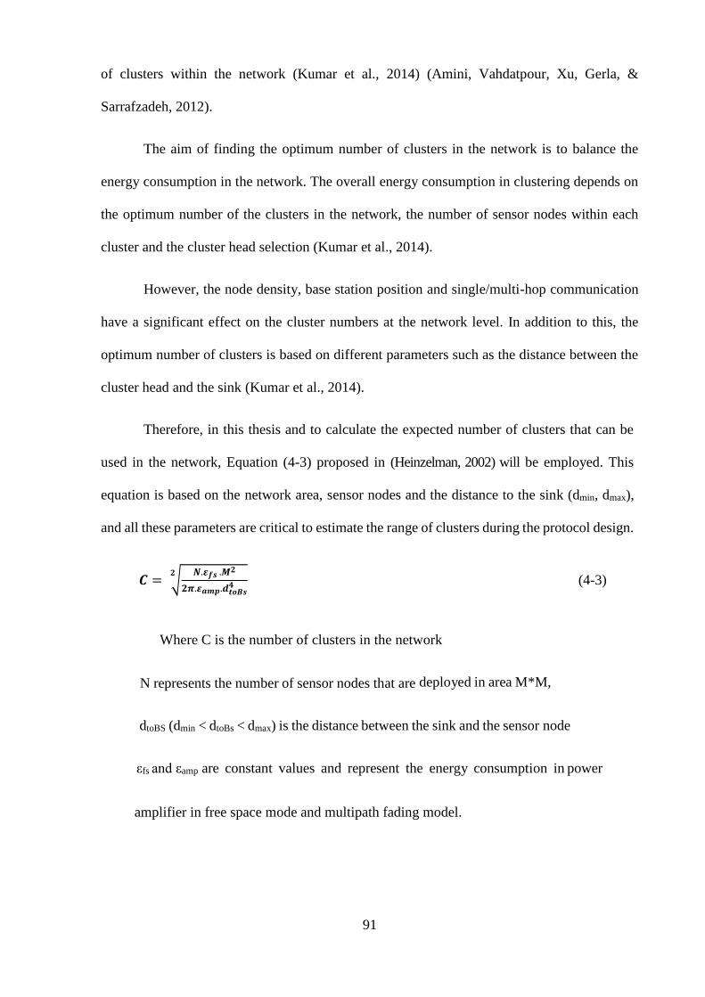
91
of clusters within the network (Kumar et al., 2014) (Amini, Vahdatpour, Xu, Gerla, &
Sarrafzadeh, 2012).
The aim of finding the optimum number of clusters in the network is to balance the
energy consumption in the network. The overall energy consumption in clustering depends on
the optimum number of the clusters in the network, the number of sensor nodes within each
cluster and the cluster head selection (Kumar et al., 2014).
However, the node density, base station position and single/multi-hop communication
have a significant effect on the cluster numbers at the network level. In addition to this, the
optimum number of clusters is based on different parameters such as the distance between the
cluster head and the sink (Kumar et al., 2014).
Therefore, in this thesis and to calculate the expected number of clusters that can be
used in the network, Equation (4-3) proposed in (Heinzelman, 2002) will be employed. This
equation is based on the network area, sensor nodes and the distance to the sink (dmin, dmax),
and all these parameters are critical to estimate the range of clusters during the protocol design.
𝑪 = √𝑵.𝜺𝒇𝒔 .𝑴
𝟐
𝟐𝝅.𝜺𝒂𝒎𝒑.𝒅𝒕𝒐𝑩𝒔𝟒
𝟐 (4-3)
Where C is the number of clusters in the network
N represents the number of sensor nodes that are deployed in area M*M,
dtoBS (dmin < dtoBs < dmax) is the distance between the sink and the sensor node
εfs and εamp
are constant values and represent the energy consumption in power
amplifier in free space mode and multipath fading model.
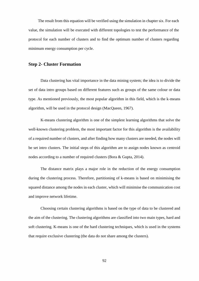
92
The result from this equation will be verified using the simulation in chapter six. For each
value, the simulation will be executed with different topologies to test the performance of the
protocol for each number of clusters and to find the optimum number of clusters regarding
minimum energy consumption per cycle.
Step 2- Cluster Formation
Data clustering has vital importance in the data mining system; the idea is to divide the
set of data intro groups based on different features such as groups of the same colour or data
type. As mentioned previously, the most popular algorithm in this field, which is the k-means
algorithm, will be used in the protocol design (MacQueen, 1967).
K-means clustering algorithm is one of the simplest learning algorithms that solve the
well-known clustering problem, the most important factor for this algorithm is the availability
of a required number of clusters, and after finding how many clusters are needed, the nodes will
be set intro clusters. The initial steps of this algorithm are to assign nodes known as centroid
nodes according to a number of required clusters (Bora & Gupta, 2014).
The distance matrix plays a major role in the reduction of the energy consumption
during the clustering process. Therefore, partitioning of k-means is based on minimising the
squared distance among the nodes in each cluster, which will minimise the communication cost
and improve network lifetime.
Choosing certain clustering algorithms is based on the type of data to be clustered and
the aim of the clustering. The clustering algorithms are classified into two main types, hard and
soft clustering. K-means is one of the hard clustering techniques, which is used in the systems
that require exclusive clustering (the data do not share among the clusters).

93
The general steps of K-means that are used during the research are shown in Figure (4-
10) and the details are as described below (Leskovec, Rajaraman, & Ullman, 2014).
1- Initialization step:
The first initial Centroid Node (CN) will be assigned randomly from the set of nodes,
as shown in Figure (4-10a, b).
From Figure (4-10c), the other CNs (based on required clusters, for example two
clusters) will be selected based on distance condition; in other words, the other initial
CNs are the nodes that have a minimum distance from the set of maximum distance to
other nodes in the network.
2- Classification step:
The other nodes will join the nearest CN (Min (d) minimum distance to it) and the
distance is calculated based on Euclidian distances (d).
3- Centroid recalculation:
Reassign new CNs using the formula (4-4) for each cluster and repeat step 2, as illustrate
in Figure (4-10d).
New CN (x,y)= ∑𝑿
𝒏,
𝒚
𝒏 (4-4)
Where x, y are the coordination of the nodes within the cluster and n is the number of the
nodes with the cluster.
4- Convergence condition:
The operation of the K-means will stop when the convergence occurs. Convergence
means the centroid node CN does not change, or cluster will not be changed as shown in
Figure (4-10 e, f).
In K-means algorithm, the convergence iterations cannot based on random or fixed
iterations because it depends on the required number of clusters and number of nodes in the

94
network. Therefore, in this thesis, as will show in chapter Six, the simulation of the K-means
will explain how these iterations are changeable.
5- Clusters Information:
The clusters table will be formed. This table contains the clusters members’ information such
as Cluster ID, Total Number of nodes in the cluster, Cluster members ID, Cluster members’
position and Cost function of cluster members.

95
Fig
ure
(4-1
0)
K-m
ean
s alg
ori
thm
(ex
am
ple
if
nu
mb
er o
f re
qu
ired
clu
ster
s in
tw
o)
(a)
nod
es s
et (
b)
firs
t in
itia
l C
N r
an
dom
ly (
c) a
noth
er C
N i
s n
od
e is
th
e fu
rth
est
nod
e (d
)
reass
ign
new
CN
(e)
new
clu
ster
s (f
) fi
nal
clu
ster

96
The general flow chart for cluster formation step illustrated in Figure (4-11).
Figure (4-11) Cluster Formation Diagram
After completing the cluster formation, the cluster head node for each node will be
selected. The full details are in the next section.
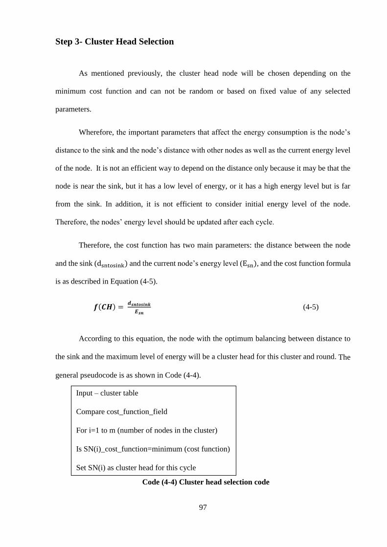
97
Input – cluster table
Compare cost_function_field
For i=1 to m (number of nodes in the cluster)
Is SN(i)_cost_function=minimum (cost function)
Set SN(i) as cluster head for this cycle
Step 3- Cluster Head Selection
As mentioned previously, the cluster head node will be chosen depending on the
minimum cost function and can not be random or based on fixed value of any selected
parameters.
Wherefore, the important parameters that affect the energy consumption is the node’s
distance to the sink and the node’s distance with other nodes as well as the current energy level
of the node. It is not an efficient way to depend on the distance only because it may be that the
node is near the sink, but it has a low level of energy, or it has a high energy level but is far
from the sink. In addition, it is not efficient to consider initial energy level of the node.
Therefore, the nodes’ energy level should be updated after each cycle.
Therefore, the cost function has two main parameters: the distance between the node
and the sink (dsntosink) and the current node’s energy level (Esn), and the cost function formula
is as described in Equation (4-5).
𝒇(𝑪𝑯) = 𝒅𝒔𝒏𝒕𝒐𝒔𝒊𝒏𝒌
𝑬𝒔𝒏 (4-5)
According to this equation, the node with the optimum balancing between distance to
the sink and the maximum level of energy will be a cluster head for this cluster and round. The
general pseudocode is as shown in Code (4-4).
Code (4-4) Cluster head selection code

98
A cluster head table will be formed containing:
1- Cluster number
2- CH ID
3- CH position
4- CH distance to sink
4-3-3-2 Setup Stage (prepare the necessary data for transmission to the
nodes)
Once the optimum number of clusters and their members are found, the server will send
a Server to Sink Cluster Information Packet (Cl_Inf_Server_sink_PDU) to the sink, as shown
in Figure (4-12). This packet contain the full information for the clustering. Description of this
packet’s fields is found in Appendix A.
Figure (4-12) Server to Sink Cluster Information Packet (Cl_Inf_Server_sink_PDU)
The sink in turn and after receiving this packet, will send it to the nodes using a Sink
to Node Cluster Information Packet (Cl_Inf_Sink_Node_PDU) as in Figure (4-13).
Description of this packet’s fields found in Appendix A

99
After receiving the clustering information, if the node role is as CH, it will be in on
mode, while if it is as cluster member, it will turn off and waiting for their time slot to transmit
the data.
Figure (4-13) Sink to Node Cluster Information Packet (Cl_Inf_Sink_Node_PDU)
4-3-3-3 Steady State stage (data transmission)
In this stage, the sensor nodes will start their sensing activity and transmit the sensed
data to cluster head nodes once per cycle according to a certain time slot defined by the NFV
server. The cycle numbers depend on the number of clusters in the network. However, the
cycle time depends on the number of sensor nodes within the cluster. For each cycle, the cluster
head node will send its data at the end of the cycle, the sensed data Info (Sense_Data_Info)
shown in Figure (4-14) and the full details is in Appendix A.
Figure (4-14) Sensed Data Info (Sense_Data_Info)
Once all sensed data from the sensor nodes in the cluster have been received, and before
transmission process to the sink, the cluster head performs data aggregation on the data and
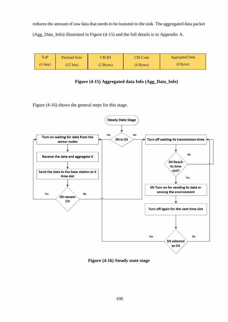
100
reduces the amount of raw data that needs to be transmit to the sink. The aggregated data packet
(Agg_Data_Info) illustrated in Figure (4-15) and the full details is in Appendix A.
Figure (4-15) Aggregated data Info (Agg_Data_Info)
Figure (4-16) shows the general steps for this stage.
Figure (4-16) Steady state stage

101
4-3-4 Schedule Formation
After selecting the cluster head nodes and specifying the nodes for each cluster, the
NFV server will create a TDMA schedule that is based on the number of nodes within the
cluster. The schedule will be used to inform the nodes when they should send their data to the
cluster head node. In addition, the same process will be done for cluster head nodes, and the
NFV server will form a schedule table for cluster head nodes to know their transmission time
to the base station. This process will lead to reduce the number of collisions in the network.
Furthermore, to help the non-cluster nodes to distinguish their cluster head and reduce
the amount of interference between the clusters, a unique code will be assigned to each head
node by the server, and the non-cluster nodes will use this code during the data transmission to
their corresponding head node. Furthermore, the cluster head node will use this code during the
communication with the sink.
The sink will send End Cycle Notification Packet (End_Cycle_notify_PDU)to inform
the server the end time for the current cycle. This packet shown in figure (4-17) and full details
of this packet is in Appendix A.
Figure (4-17) Notification Packet (Notification_PDU)

102
4-4 Energy Consumption Calculation Function
After completing the cluster formation and cluster head selection, and the clustering
details have been sent to the nodes, the server starts to monitor and manage the networks by
estimating the amount of energy consumption (Econsumed) based on the developed mathematical
model. The details of the estimation model will be explained in chapter five.
The current energy level of the cluster head node will be checked to find whether it
should be changed or not for the current cycle. The current energy level of the node (Ecurrent)
will be found by the Equation (4-6)
Ecurrent = EPrevious-Econsumed (4-6)
Where EPrevious is the energy level of the node
The values of Ecurrent, EPrevious and Econsumed will be organised in an energy table that will
be updated at each cycle. The contains of energy table are:
1- Node’s ID
2- Node’s current energy level
3- Node’s energy consumption in current cycle
4- Node’s energy level from previous cycle
As mentioned previously, it is important to find the optimum number of clusters within
the network during the protocol operation. Therefore, the energy consumption/cycle will be
calculated with the different value of C and different network topologies to find the optimum
number of clusters in the network based on minimum energy consumption.
103
4-5 Cluster Head re-selection Function
According to the assumption in this thesis, the time for the node to be a cluster head is
not fixed and different from cluster to cluster because it depends on the number of nodes in the
cluster, transmission bit rate, and the data packet size.
Most of the previous studies in the clustering technique were based on a fixed time for
the re-cluster head selection or re-clustering processes. The round time calculation in these
studies depend on the initial number of nodes and then make it fixed for the whole network
operation. However, this approach is inefficient because of the nature of the sensor network,
which is dynamic, meaning the number of nodes may be changed. Therefore, fixing the round
time leads to unbalancing the network load and this will affect its performance.
The server will monitor the energy level of the current cluster head node and check it at
the end of each cycle to avoid draining the cluster head energy as shown in Figure (4-18). The
new cycle for each cluster will be started under certain conditions, which is based on a triggered
process; this means that there will be an energy level threshold, as illustrated in equation (4-7)
𝐸threshold = 𝐸𝑎𝑣𝑔
2⁄ (4-7)
Where: Eavg represents the average of the sensor nodes’ current energy level in the
cluster.
It is important to know that the cluster head selection process is distributed among all
nodes, which means that the node that will be selected as the cluster head for the current round
will be eliminated and not chosen as the cluster head for any new cycle.

104
Figure (4-18) Cluster Head re-selection Function
The server will send a Server to Sink Cluster Head re-selection Packet
(Reslect_CH_Server_Sink_Packet) , that shown in figure (4-19), contain the information for
the new cluster heads for the clusters that should change it CH.
Figure (4-19) Cluster Head re-selection Packet (Reslect_CH_Packet)

105
The sink will forward this packet using a Sink to Node Cluster Head re-selection Packet
(Reselect_CH_Sink_Node_PDU), shown in Figure (4-20), to the nodes. Full details of these
packets is in Appendix A.
Figure (4-20) Cluster Head re-selection Packet (Reslect_CH_Sink_Node_Packet)
4-6 Re-Clustering Function
Finally, managing the re-clustering process affects the network lifetime, and therefore,
it is essential to know when the clusters should be reformed. For the proposed protocol, the re-
clustering process will be initiated again when all sensor nodes within the cluster have been
elected as a cluster head. As mentioned previously, the new energy level for the nodes will be
calculated by the server based on the proposed mathematical model that will be explained in
the next chapter. The activity diagram for this function is shown in Figure (4-21).

106
Figure (4-21) Re-Clustering Function
4-7 Summary:
The PDU protocol diagram and the overall flow chart for the VCR protocol description
are illustrated in Appendix B and C respectifly.
The general steps of the proposed protocol have been explained in detail in this chapter.
A full flow chart had been drawn to explain the general behaviour of the protocol.
The new protocol (VCR) differs from other clustering based routing protocols in the
clustering formation process that occurs before other steps, while in other protocols, the cluster
formation is done before the cluster head selection.
In clustering, centralised clustering is more efficient than distributed clustering, so it is
crucial to determine the optimum number of clusters and which node will be selected as a cluster
head to minimise the protocol complexity and improve energy efficiency.

107
The optimum number of clusters is found based on an optimisation process, which is
the amount of energy consumption per cycle. Also, it improves the clustering process by
adopted the idea of the k-means (clustering algorithm).
It is also noted that the selection of the cluster head is not random; it depends on a cost
function that combines the distance of the node to sink and its current energy level. This is more
efficient than just using the distance nodes because it is possible that the node is near the sink
but has a low level of energy, or it has a high energy level but is far from the sink. Therefore,
the nodes with a minimum cost function, which implies the best balancing between distance to
sink and maximum energy level, will be a cluster head.
The rotation of cluster head role (reselect CH) will be a process trigged by an energy
threshold, and this will improve the network’s overall lifetime by increasing the time for the
node to be CH and distributing the selection among the nodes. The next chapter will present the
developed mathematical model of the proposed protocol.
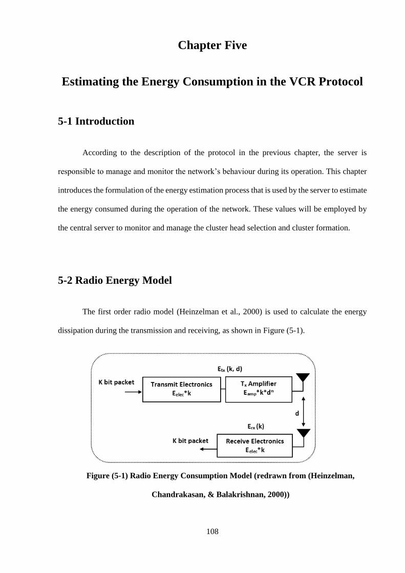
108
Chapter Five
Estimating the Energy Consumption in the VCR Protocol
5-1 Introduction
According to the description of the protocol in the previous chapter, the server is
responsible to manage and monitor the network’s behaviour during its operation. This chapter
introduces the formulation of the energy estimation process that is used by the server to estimate
the energy consumed during the operation of the network. These values will be employed by
the central server to monitor and manage the cluster head selection and cluster formation.
5-2 Radio Energy Model
The first order radio model (Heinzelman et al., 2000) is used to calculate the energy
dissipation during the transmission and receiving, as shown in Figure (5-1).
Figure (5-1) Radio Energy Consumption Model (redrawn from (Heinzelman,
Chandrakasan, & Balakrishnan, 2000))

109
From the above figure, the power attenuation depends on the distance between the
transmitter and receiver. The distance parameter (dn) is based on the channel path loss, which
is either free space (d2) used for the short distance communication or multi fade path (d4) that
is used for long distance communication.
Accordingly, the formula for sending a k-bit data to a distance d is
𝐸𝑡 = 𝐸𝑒𝑙𝑒𝑐 ∗ 𝑘 + 𝜀𝑎𝑚𝑝 (𝜀𝑓𝑠) ∗ 𝑘 ∗ 𝑑𝑛 (5-1)
While the formula for receiving a k-bit data is
𝐸𝑟 = 𝐸𝑒𝑙𝑒𝑐 ∗ 𝑘 (5-2)
Where
Et= energy consumption formula to transmit k-bit data to a d distance,
Er=energy consumption formula to receive a k-bit data,
k= packet size (bit),
dn= distance between two sensor nodes or sensor node and the sink,
n is the path loss exponent, which is specified by the radio propagation model (n=2 in free
space model and d<d0 (between sensor nodes and cluster head) or n=4 in two ground model
and d>=d0 (between cluster head node and the sink), depending on the distance between
sender and receiver),
Eelec= transmitter and receiver electronics = 50 nJ/bit,
εfs = energy consumption in power amplifier in free space mode, used if d<do = 10 pJ/bit/m2
(if n=2),

110
𝜀𝑎𝑚𝑝= energy consumption in power amplifier in multi path fading, used if d>do= 0.0013
pJ/bit/m4 (if n=4), do=87.7 m (√εfs
εamp
(Wendi Beth Heinzelman, 2002) (Heinzelman et al.,
2002).
5-3 Analysis of the Energy Consumption of the VCR Protocol
As discussed previously in Chapter two, the sensor node consumes its energy to perform
different types of activity such as processing, sensing and communications. In the
communications domain, the node may be in four different modes: transmit mode, receive
mode, idle mode and sleep mode. On the other hand, the node modes during the processing are
on, off and idle, while in sensing, the nodes can be either in on mode or off mode.
According to this, the mathematical model of the proposed protocol will take into
consideration all these fields and activities during the design process. In order to understand the
main contents of the mathematical model, Figure (5-2) illustrates the general map for energy
consumption fields, which (a) is for cluster head mode and (b) for non-cluster head mode. The
general Equations for the nodes in either cluster head mode or cluster member mode is
illustrated in Equations (5-3) and (5-4) respectively.
For cluster head mode
Etotal/ch/ cycle = Ech/ cycle + Ebroadcast/sn (5-3)
Where Ech/ cycle is the cluster head mode energy consumption and Ebroadcast/sn is the broadcasting
energy consumption.
While For cluster member mode
Etotal/sn/ cycle = Esn/ cycle + Ebroadcast/sn (5-4)
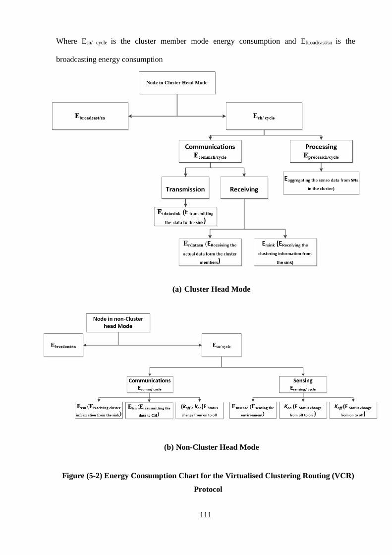
111
Where Esn/ cycle is the cluster member mode energy consumption and Ebroadcast/sn is the
broadcasting energy consumption
(a) Cluster Head Mode
(b) Non-Cluster Head Mode
Figure (5-2) Energy Consumption Chart for the Virtualised Clustering Routing (VCR)
Protocol
112
5-3-1 Energy Consumption in Node Discovery (Broadcasting)
As mentioned in chapter four, to start the protocol operation, the sensor nodes should
send their information to the sink that will forward it to the NFV server to initiate the clustering
function (knows as node discovery).
During this step, the nodes will be assumed to send their information to the sink with
transmission power that is equal to the transmission power of the farthest node in the network
(node with the greatest distance from the sink).
In this case, Equations (5-5) and (5-6) will be used during this process whether the
system is free space or multi-path.
Else
Where dmax is the distance from the farthest node to the sink
do= √εfs
εamp
that is approximately = 87.7 m.
Moreover, in order to estimate the energy consumption of the whole network, Equation
(5-7) represents the formula that uses
Ebroadcasr/netwoerk=sn* Ebroadcast/sn (5-7)
where sn is the number of nodes in the network.
Ebroadcast/sn =Eelec∗ k +εfs*k*d2max
when dmax <do (5-5)
Ebroadcast/sn =Eelec∗ k +εfs*k*d4max
when dmax >do (5-6)

113
The energy consumption in this step will be taken into account during the initiated cycle
only as the nodes send their information in this cycle and do not need to resend it again. The
next sections discuss the formulation of the mathematical models, as nodes will either be a
cluster head mode or cluster member mode.
5-3-2 Cluster Head (CH) node energy consumption per cycle:
In this section, a mathematical equation for the cluster head node is derived. Once the cluster
head node is selected by the server, it will be on all the time during the protocol operation. The
main functions of a cluster head will be receiving the sensed data from its members, processing
these data (aggregate the data) and then sending it to the sink according to its time slot.
According to this, the energy consumed by a cluster head node (Ech) is (Ecommch/cycle) during
the communication domain and (Eprocessch/ cycle) during the processing domain (aggregate the
received data). Therefore, the total energy consumed by the cluster head in each cycle is Equation
(5-8).
Ech/cycle= Ecommch/cycle +Eprocessch/cycle (5-8)
Where
For communication domain, the cluster head’s energy will dissipate while receiving the
clustering information from the sink, receiving the sensed data from the cluster members within
their time slots, and transmitting the sensed data to the sink at the end of each cycle. Hence,
Equation (5-9) represents the energy consumed in transmitting every cycle.
Ecommch/ cycle =𝐸𝑟𝑠𝑖𝑛𝑘 + ∑ 𝐸rdatasn (𝑚) +𝑖𝑚=1 Etdatasink (5-9)

114
where i is the number of nodes within the cluster.
Ersink is the energy consumed during receiving cluster information from the sink.
Erdatasn is the energy consumed during receiving the sensed data from the cluster
member
Etdatasink is the energy consumed during transmit the sensed data to the sink
By replacing Ecommch/ cycle with (5-9), Equation (5-10) will represent the energy consumption
during the clustering stage.
Ech/ cycle =𝐸𝑟𝑠𝑖𝑛𝑘 + ∑ 𝐸rdatasn (𝑚) +𝑖𝑚=1 Etdatasink + Eprocessch/cycle (5-10)
On the other hand, at the end of each cycle, the server will monitor the energy of the
cluster head node to determine whether it is below a threshold or not. So the Ersink will be
calculated when the new clustering information is received.
In addition to that, the amount of energy consumption for each node (Ebroadcast/Sn) in
broadcasting will be added at the beginning of the initial cycle.
5-3-3 Non-Cluster Head energy consumption per cycle:
All non-cluster head nodes after receiving the clustering information, will be turned off
and remain off until turned back on depending on the application type and reaching its time slot.
Therefore, in this mode, the sensor node’s energy will be consumed in communication and
sensing domains, as shown in Equation (5-11).
Esn/ cycle =Ecomm/ cycle +Esensing/ cycle (5-11)

115
Where
Ecomm/ cycle is the energy consumption in communication
Esensing/ cycle is the energy consumption in sensing.
For the first field, the node will transmit the sensed data to its cluster head according to
its time slot and once at each cycle, it will receive the clustering information from the sink. The
energy consumption equations in this domain will be as in Equation (5-12)
Ecomm/ cycle =𝐸𝑡𝑠𝑛 + 𝐸𝑟𝑠𝑛 + 𝑘𝑜𝑓𝑓 + 𝑘𝑜𝑛 (5-12)
Where Etsn is the energy consumed during data transmission to the cluster head
Ersn is the energy consumed during receiving clustering information from the sink.
The status change energy consumption in communication will include two cases:
- From on to off at the end of receiving process (𝑘𝑜𝑓𝑓)
- From off to on in order to transmit the data (𝑘𝑜𝑛)
Furthermore, part of the sensor node’s energy will be consumed during the sensing activity;
hence the complete model for calculating the amount of energy consumption will be as shown
in Equation (5-13).
Esensing/ cycle =∑ 𝐸𝑠𝑛𝑠𝑒𝑛𝑠𝑒𝑝𝑙=1 + 𝑘𝑜𝑓𝑓 + 𝑘𝑜𝑛 (5-13)
Where 𝐸𝑠𝑛𝑠𝑒𝑛𝑠𝑒 is the energy consumed during the sensing activity
𝑘𝑜𝑓𝑓 and 𝑘𝑜𝑛 are as described above
P is the number of sense activities.
116
By combining (5-12) and (5-13), the amount of energy consumption for the cluster member
node will be formulated, as shown in Equation (5-14).
Esn/ cycle =∑ 𝐸𝑡𝑠𝑛(𝑐) + 𝐸𝑟𝑠𝑛𝑏𝑐=1 +∑ 𝐸𝑠𝑛𝑠𝑒𝑛𝑠𝑒(𝑙)𝑝
𝑙=1 + 2𝑘𝑜𝑛+2𝑘𝑜𝑓𝑓 (5-14)
As in cluster head mode, the node will receive the clustering information only if new
clustering occurs so that Ersn will be performed in this case, and the amount of energy
consumption for each node (Ebroadcast/Sn) in the broadcasting step will be added at the beginning
of the initial round.
5-3-4 Remaining energy level for CHs and Cluster members’ (CM) nodes:
As mentioned previously in chapter four, the server will monitor the nodes’ energy
consumption at each cycle in order to estimate their energy level. Therefore, The NFV server
will calculate and update the amount of remaining energy for cluster members (CM) and cluster
head (CH) node per cycle using Equations (5-15) and (5-16) respectively.
If the node is cluster member
Ecurrent/ cycle =Eprevious-Etotal/sn/cycle (5-15)
If the node is cluster head
Ecurrent/ cycle =Eprevious – Etotal/ch/ cycle (5-16)
Where Eprevious is the energy level of the nodes at the previous cycle

117
5-3-5 Total Cluster Energy Consumption per Cycle:
After estimating the energy consumption for each node, the energy consumption for a
single cluster will be the summation of the energy consumption for the cluster members and
cluster head nodes, as in Equation (5-17).
𝐸𝑡𝑜𝑡𝑎𝑙𝑐𝑙𝑢𝑠𝑡𝑒𝑟/𝑐𝑦𝑐𝑙𝑒 = Ech/ cycle + ∑ Esn/cycle𝑐𝑙𝑠𝑛𝑖=1 (5-17)
Where clsn is the number of nodes in the cluster.
5-3-6 Total Network Energy Consumption per Cycle:
In order to estimate the amount of energy consumption for the whole network, the total
energy consumption for the network will be the summation of the energy consumption of all
clusters within the network, as in Equation (5-18).
Etotalnet/ cycle = ∑ (Etotalcluster/cycle)𝑖 𝐶𝑖=1 (5-18)
Where C: the total number of clusters within the network and Etotalnet/cycle is the energy
consumption for a cluster per cycle.
5-4 Analysis of power consumption in the LEACH protocol
To understand the clustering function and the number of communications during this
function, the behavioral of LEACH protocol in terms of number of communications will be
analysed mathematically in order to compare between the VCR and LEACH protocols.
According to the details and communications diagram of LEACH protocol mentioned in Chapter
118
3, Figure (3-8), a sensor node consumes its energy to perform various activities, such as
clustering, processing and sensing.
The general Equations for the nodes in either cluster head mode or cluster member mode
is illustrated in Equations (5-19) and (5-20) respectively.
If the node’s role is clsuter head
Echtotal = Ecommch + Eprocesstotal + Eagg (5-19)
Where Ecommch is the energy consumption in communication field
Eprocesstotal is the energy consumption in processing activities
Eagg is the energy consumption in data aggregation
However, if the node is a cluster member
Esntotal=Ecommsn+ Esensing + Eprocesstotal (5-20)
Where Ecommsn is the energy consumption in communication field
Eprocesstotal is the energy consumption in processing activities
Esensing is the energy consumption in sensing
5-4-1 Energy Consumption in Processing
The first energy consumption domain for the nodes in LEACH will be the consumption
that occurs during the processing where the necessary information should be calculated and
checked to build the clusters. Hence, the nodes consume energy in order to perform various
processing activities as processing to generate the random value (r) between 0 and 1, processing

119
to calculate the threshold value (TH), and processing to check whether the node is a cluster head
or not.
Hence, the energy consumption equation for this step is shown in Equation 5-21:
Eprocesstotal=Eprocessrand+Eprocessth+Eprocrsscheck (5-21)
Where
Eprocessrand is energy consumption for random value generation
Eprocessth is energy consumption for threshold calculation
Eprocrsscheck is energy consumption for checking
Moreover, the node consumes its energy in the communication field to perform
transmission with other sensor nodes and receiving from the sink or other sensor nodes. After
completing the processing, the next function for the sensor node will be the clustering. In
clustering, the sensor node will be responsible for the cluster head selection and cluster
formulation.
As in the proposed protocol, the sensor node mode can be in two different modes; either
cluster head mode or non-cluster head mode.
5-4-2 Energy Consumption for Cluster Head Mode:
In this case, the sensor node will be treated as cluster head; therefore, its energy will be
dissipated in communication and processing and data aggregation.
The energy consumption in communication field contains various transmitting activities.
For instance, transmitting the CH announcement to other SNs, transmitting the time slot to the
cluster memebrs, transmitting the CH announcement to the sink, transmitting the sensed data to

120
the sink), receiving activities such as receiving the join request from other SNs, receiving the
sensed data from the cluster members and receiving its time slot from the sink.
For Eprocesstotal represent the processing energy consumption as illustrated in Equation 5-
21. While Eagg is the data aggregation energy consumption
The final Equation for this field is as shown in (5-22).
Ecommch= Etanc + ∑ Ettime𝑧𝑚=1 (𝑚) + Etsink + Etdata + ∑ Erjr
𝑤𝑗=1 (𝑗) + ∑ Erdata
𝑑𝑎=1 (𝑎) + Etimesink
(5-22)
Where z = the number of transmissions for the time slot packet sent from CH (which is based
on the total number of sensor nodes within the cluster),
d = the amount of received sensed data (which relies on the total number of cycle
within the cluster),
w = the number of join requests received from the sensor nodes to join the cluster.
Etanc = the energy consumption for transmitting the CH announcement to other SNs
Ettime = the energy consumption for transmitting the time slot to the cluster memebrs
Etsink = the energy consumption for transmitting the CH announcement to the sink
Etdata = the energy consumption for transmitting the sensed data to the sink
Erjr = the energy consumption for receiving activities such as receiving the join request
from other SNs)
Erdata = the energy consumption for receiving the sensed data from the cluster members
Etimesink = the energy consumption for receiving SN time slot from the sink.

121
By substituting the formulas of Equations (5-21) and (5-22) in Equation (5-19), the new
equation for the energy consumption is as shown in Equation (5-23).
Echtotal =
Eprocessrand+Eprocessth+Eprocrsscheck+Etanc + ∑ Ettime𝑧𝑚=1 (𝑚) + Etsink + Etdata + ∑ Erjr
𝑤𝑗=1 (𝑗) +
∑ Erdata𝑑𝑎=1 (𝑎)+Etimesink+Eagg (5-23)
5-4-3 Energy Consumption for non-Cluster Head Mode:
Meanwhile, for the other mode, which is a cluster member, energy consumption’s
includes the communication and sensing activities.
The fields of the transmitting and receiving activities performed by the node are as
follows: transmitting the join request, transmitting the sensed data to the cluster head, receiving
the CH announcement and receiving its time slot for transmission, as illustrated in Equation (5-
24)
Ecommsn = Etjr + ∑ 𝐸𝑟𝑎𝑛𝑐𝑏𝑘=1 (𝑘) + ∑ 𝐸𝑡𝑑𝑎𝑡𝑎𝐶𝐻 (𝑠)
𝑓𝑠=1 + Ertime + koff + kon (5-24)
Where
Etjr is the energy consumption for transmitting the join request
EtdataCH is the energy consumption for transmitting the sensed data to the cluster head
Eranc is the energy consumption for receiving the CH announcement
Ertime is the energy consumption for receiving its time slot for transmission
b is the number of receiving the CH announcements
f is the number of data transmissions

122
Furthermore, the energy consumption during the status change will be assumed as a
constant value, e.g. the status change from on to off (koff) (turn off after joining a cluster) and a
status change from off to on (kon) (turn on when an event occurs, or it is time for transmission).
In the same way, the sensor node will consume its energy in the sensing activity. To
calculate this amount, Equation (5-25) will be used:
Esensing=∑ 𝐸𝑠𝑛𝑠𝑒𝑛𝑠𝑒(𝑔)𝑝𝑔=1 + koff + kon (5-25)
Where 𝐸𝑠𝑛𝑠𝑒𝑛𝑠𝑒 is the energy consumed during the sensing activity
P = the number of sense activities
The status change energy consumption in communication will include two cases and as
described previously, 𝑘𝑜𝑓𝑓 and 𝑘𝑜𝑛.
On the whole, for the sensor node in the network, the energy consumption formula is as
shown in Equations (5-26)
Esntotal= Eprocessrand +Eprocessth +Eprocrsscheck + Etjr + ∑ 𝐸𝑟𝑎𝑛𝑐𝑏𝑘=1 (𝑘) + ∑ 𝐸𝑡𝑑𝑎𝑡𝑎𝐶𝐻 (𝑠)
𝑓𝑠=1 + Ertime +
∑ 𝐸𝑠𝑛𝑠𝑒𝑛𝑠𝑒(𝑔)𝑝𝑔=1 +2koff+ 2kon (5-26)
By analysing the mathematical models for the proposed protocol (VCR) and LEACH
during the clustering function and in terms of the number of communications (the amount of
transmission and receiving), it showed that there is a reduction in the number of
communications during the clustering function between the two protocols for the cluster head
node and cluster member, as described in Table (5-1).

123
For the proposed protocol, the cluster head node has three communications (received or
transmitted), while in LEACH there are seven, which means that there is a 42.85% reduction
in the number of communications and this will affect the total amount of energy consumption
for the node.
Furthermore, for the cluster member node, the reduction is approximately 50%, because
in the proposed protocol the nodes have two communication activities compared with four in
LEACH.
Table (5-1) Number of Communications for VCR and LEACH
5-5 Summary
According to previous explanation, the proposed protocol (VCR) based on the centralised
operation where the server will be responsible for the network management during the protocol
operation as well as estimate the node’s energy consumption during the clustering process based
on an energy estimation model.
The purpose of the analytical model is to estimate the amount of energy consumption
during the network’s operations. The mathematical model takes into account the general fields
that the nodes consume its energy on such as transmission, receiving and status change.
Node Mode Number of Communications in
in VCR
Number of Communications in
LEACH
Cluster Head 3 7
Cluster Member 2 4

124
Moreover, in order to find the percentage of the communication reduction in term of
number of communications for the nodes, a mathematical model based on the communication
operation of the LEACH protocol had been derived and explained.
125
Chapter Six
Simulation, Validation and Evaluation
6-1 Introduction
This chapter discusses the simulation of the VCR protocol and the validation and
evaluation. The simulation was based on the MatlabR2016a environment, which is a high-level
language and interactive environment for numerical computation, visualisation, and
programming.
As described in chapter four, after completing the cluster formation and the cluster head
selection, the energy consumption/cycle was calculated. This procedure was repeated for
different topologies and parameters to find the average values of the energy consumption to be
used for the validation and evaluation steps.
6-2 Experimental Design
6-2-1 Validation Experiments:
The aim of the validation process is to determine the efficiency of the proposed protocol
in minimising the amount of energy consumption of the sensor nodes under various conditions
and, thus, improving network lifetime. To validate the behaviour of the proposed protocol, it
will be tested under different experiments, as listed:
1- Experiment One: The simulation is repeated for a varied number of clusters, with the
number of nodes of 100 to find the optimum number of clusters in terms of minimum
energy consumption per cycle.

126
2- Experiment Two: After the optimum number of clusters have been found and fixed, and
the operation will be tested depending on:
- Sensing area (for various area sizes (100*100) and (500*500)).
- Sink Position (Placing the sink position inside or outside the sensing
environment).
3- Experiment Three: the optimum number of clusters for different number of nodes
(n=50,150,200) will be found and verified by comparing it with the data from the
mathematical analysis.
4- Experiment Four: The amount of energy consumption will be measured based on
various node density (by fixing the area size and changing the number of nodes deployed
in the sensing area) (N=50,100,150,200).
5- Experiment Five: network lifetime was measured based on First Node Dead (FND)
under dynamic and static clustering for the proposed protocol.
6-2-2 Evaluation Experiments:
1- In the evaluation, the proposed protocol was tested to find whether the research objective,
which is improving the network lifetime, had been achieved or not. This was done by:
- Experiment Six: Comparing the results obtained from the proposed protocol, which is
the First Node Dead (FND) measurement simulation with the existing clustering based
protocols results, which are LEACH (for distributed type) and LEACH-C (for
centralised type).
2- Furthermore, an additional experiment (Experiment Seven) was simulated in order to
investigate the costs of the start-up stage in, LEACH and LEACH-C.
3- Finally, in terms of static clustering, Experiment Eight investigates the difference in terms
of FND between static VCR and static LEACH.

127
6-3 Network Topology Setup:
The aim of the simulation is to test the protocol operation and measure the amount of
energy consumption per cycle for the network during the protocol operation with various
topologies and parameters such as a different number of nodes, sink position and sensing area.
The basic parameters used are as shown in the Table (6-1).
The implementation began with the sensor nodes that distributed randomly in two
dimensions sensing area in the simulation environment of M * M area size. As mentioned
previously, the nodes will be in fixed position as soon as it is deployed. The pseudo codes for
sensor node and sink deployment are as shown in code (6-1).
As mentioned previously, the sink will be initialised with the size of the network
(number of nodes in the network).
Figure (6-1) is an example of the implemented network topologies, and the full
topologies and their seeds are in Appendix D.
Code (6-1) Pseudo Codes for Sensor Node and Sink Deployment
%Define network area (MxM)=Xm,Ym
For i =1 to total number of node (N)
Xsn coordination of node(i) = rand(Xm);Ysn coordination of node (i)=rand(Ym)
Node type=’N’=ordinary sensor node
%For sink position
Xsink coordination for sink=Xm/2 ; Ysink coordination for sink=Ym+75 (for
outside)
Xsink coordination for sink=Xm/2 ; Ysink coordination for sink=Ym/2 (for inside)

128
Table (6-1) Simulation Parameters
Parameters Values
εfs =energy consumption in power amplifier in free space
mode (short distance), its used if dn<d0 (if n=2)
10 pJ/bit/m2
Eelec 50 nJ/bit
Packet Size 4000 bit
εamp= energy consumption in power amplifier in two ground
model (long distance), its used if dn>d0 (if n=4)
0.0013
pJ/bit/m4
do is the threshold distance between the sender and the
receiver and its depend if the channel propagation is free
space model or two ray ground model
87.7 m
Bit rate 1 Mbps
Initial Energy 2 J
Energy to aggregate 1 bit 5 nJ/bit/signal
Figures (6-1) Network Topology Example

129
6-4 Calculation of the Optimum Number of Clusters
As explained in chapter four, if the number of clusters within the network is less or more
than the optimum value, will led to increase the energy consumption and this will affect the
network lifetime. Therefore, the aim of calculating the optimum number of clusters in the
network is to minimise the protocol complexity and energy consumption and improve the
network lifetime. After completing the calculation process, the server starts to find the expected
number of clusters (C), and this is done using Equation (4-5), as mentioned in chapter four.
For the various parameters used during the simulation process, the expected number of
clusters for each case is as shown in Table (6-2). The simulation aims to run the protocol for
each value of C in order to verify these values.
Table (6-2) Range of Clusters
Area 100 * 100 , Sink coordination (50,175)
Number of Nodes Expected range of optimum number of clusters
50 1< C < 4
100 1< C < 6
150 1 < C < 7
200 1 < C < 8
The simulation results of the following parameters will be used to compare with LEACH
and LEACH-C:
1- Number of Nodes (n=100).
2- Network area size (100*100).
3- Sink position outside the sensing area (50,175)
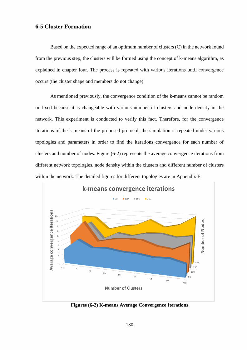
130
6-5 Cluster Formation
Based on the expected range of an optimum number of clusters (C) in the network found
from the previous step, the clusters will be formed using the concept of k-means algorithm, as
explained in chapter four. The process is repeated with various iterations until convergence
occurs (the cluster shape and members do not change).
As mentioned previously, the convergence condition of the k-means cannot be random
or fixed because it is changeable with various number of clusters and node density in the
network. This experiment is conducted to verify this fact. Therefore, for the convergence
iterations of the k-means of the proposed protocol, the simulation is repeated under various
topologies and parameters in order to find the iterations convergence for each number of
clusters and number of nodes. Figure (6-2) represents the average convergence iterations from
different network topologies, node density within the clusters and different number of clusters
within the network. The detailed figures for different topologies are in Appendix E.
Figures (6-2) K-means Average Convergence Iterations

131
From these Figure, it is concluded that the number of iterations is not fixed and it
changes based on various parameters such as nodes position, the number of clusters within the
network as well as the nodes density within the clusters.
6-6 Results and Validation
As mentioned previously, the validation of the proposed protocol includes various
experiments in order to test the network’s behavior based on the average energy consumption
per cycle. These test experiments will be described in the next sections.
6-6-1 Energy Consumption Calculation
After the clustering function (cluster formation and cluster head selection) are
completed, the clustering information will be sent to the nodes via the sink in order to start the
operation.
As mentioned previously, the server’s responsibility is to monitor the network
behaviour, cluster heads and member nodes’ energy level in order to update the information
and clustering process. This will be done based on the proposed mathematical model to
calculate the amount of energy consumption for the sensor nodes.
The energy consumption per cycle has been calculated using the proposed mathematical
model, the calculation procedure was repeated for different network topologies, and the average
values of the energy consumption were found and used during the evaluation step. As regards
the optimum number of clusters in the network, the optimum number of clusters will be found
and verified.

132
As mentioned previously, the protocol will be tested with different experiments, as
follows:
1- Experiment One: number of nodes 100, sink location 50,175 and sensing area size
(100*100):
In this experiment, the network consists of 100 nodes deployed randomly in the 100*100
sensing area. The test is based on 15 different topologies with a number of clusters between (1
to 10). The aim of this scenario is to find the optimum number of clusters based on minimum
energy consumption per cycle, and verify the values in a Table (6-2). The result is shown in
Figure (6-3).
Figure (6-3) Average Energy Consumption with N=100
The line graph shows the amount of energy consumption per cycle with a different
number of clusters in the network. From this graph, the amount of energy consumption is varied
from different number of clusters within the network. For each cluster, the behaviour of the
network is changeable with the number of nodes in the clusters, the distance among the nodes
with their cluster heads as well as the distance between the cluster head nodes and the sink.

133
Furthermore, the value of an optimum number of clusters from the Table (6-2) was
verified based on the result, and the optimum number of clusters in terms of minimum energy
consumption is 3. During the rest of the simulation process, the number of clusters will be set
to 3.
In WSN, many parameters should be taken into account in the design of any protocol.
Each of these parameters affects the behaviour of the system in terms of energy consumption;
the common parameters are the number of nodes in the network, the sink position and the size
of the sensing area. Therefore, by fixing the number of the cluster to 3, the network was tested
under various conditions, such as:
Changing sink position (inside and outside sensing area)
Changing the size of the sensing area (100*100, 500*500).
The full details of these experiments are explained in the next sections.
2- Experiment Two (change Sink Position and area size):
This experiment is based on the position of the sink, which had an important impact on the
energy consumption of the network because of the communication among the cluster heads and
the sink. Therefore, the simulation was run with the following values, and the energy
consumption values of the network are as shown in Figure (6-4).
Different sink position (inside and outside the network area), its coordination is (50, 50)
and (50,175).
Number of nodes change (50,100,150,200).
The sensing area is (100*100) and (500*500).

134
Figure (6-4) Average Energy Consumption with Varying Sink Position
The Figure (6-5) represents the amount of energy consumption per cycle based on sink
position. As can be seen from the figure, the network consumed lower amounts of energy when
the sink was located inside the sensing area because the distance among the CHs and the sink
decreased and thus influenced the amount of energy consumption. The same experiment was
repeated with larger sensing area (500*500).
As illustrated in this Figure, the network had significant levels of consumption when
the sensing area size is increased because the distance among the nodes in the clusters and the
distance between the CHs and the sink increased and thus will affect the energy consumption
of the nodes. In addition, the amount of energy consumption of the network is more reliable
when the sink is located in the network area.
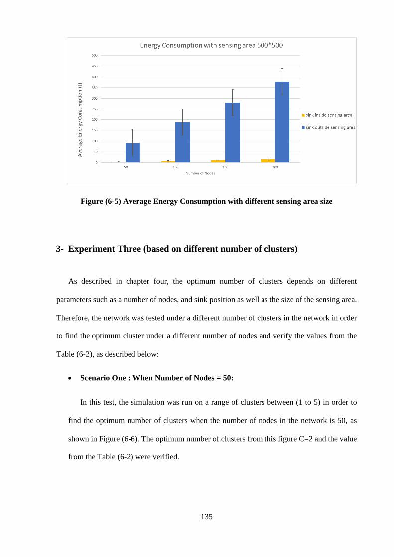
135
Figure (6-5) Average Energy Consumption with different sensing area size
3- Experiment Three (based on different number of clusters)
As described in chapter four, the optimum number of clusters depends on different
parameters such as a number of nodes, and sink position as well as the size of the sensing area.
Therefore, the network was tested under a different number of clusters in the network in order
to find the optimum cluster under a different number of nodes and verify the values from the
Table (6-2), as described below:
Scenario One : When Number of Nodes = 50:
In this test, the simulation was run on a range of clusters between (1 to 5) in order to
find the optimum number of clusters when the number of nodes in the network is 50, as
shown in Figure (6-6). The optimum number of clusters from this figure C=2 and the value
from the Table (6-2) were verified.

136
Figure (6-6) Optimum Number of Clusters for N=50
Scenario Two: When Number of Nodes = 150:
Likewise, and as in the previous scenario, the protocol was tested with 150 nodes
where the range of clusters was between (1 to 8) to find the best number of clusters in terms
of minimum energy consumption and compare it with Table (6-2) for verification. Figure
(6-7) illustrates the results of this step. From the results, the optimum number of clusters,
in this case, is 4.
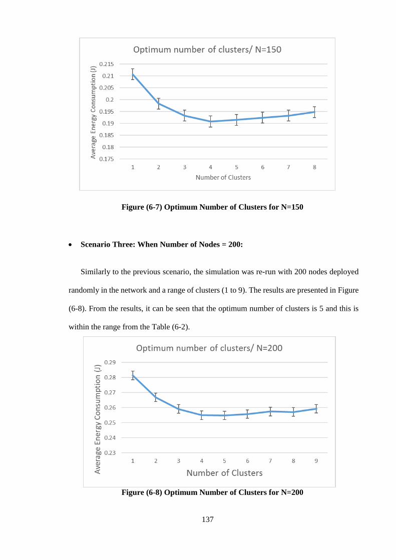
137
Figure (6-7) Optimum Number of Clusters for N=150
Scenario Three: When Number of Nodes = 200:
Similarly to the previous scenario, the simulation was re-run with 200 nodes deployed
randomly in the network and a range of clusters (1 to 9). The results are presented in Figure
(6-8). From the results, it can be seen that the optimum number of clusters is 5 and this is
within the range from the Table (6-2).
Figure (6-8) Optimum Number of Clusters for N=200
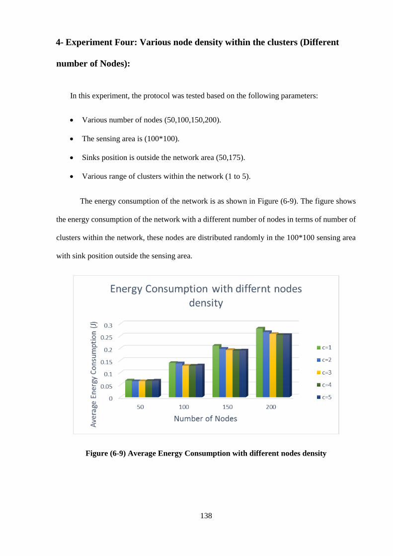
138
4- Experiment Four: Various node density within the clusters (Different
number of Nodes):
In this experiment, the protocol was tested based on the following parameters:
Various number of nodes (50,100,150,200).
The sensing area is (100*100).
Sinks position is outside the network area (50,175).
Various range of clusters within the network (1 to 5).
The energy consumption of the network is as shown in Figure (6-9). The figure shows
the energy consumption of the network with a different number of nodes in terms of number of
clusters within the network, these nodes are distributed randomly in the 100*100 sensing area
with sink position outside the sensing area.
Figure (6-9) Average Energy Consumption with different nodes density
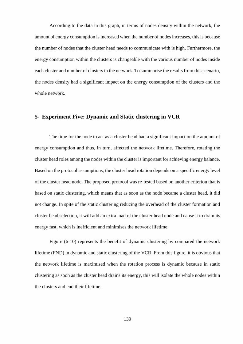
139
According to the data in this graph, in terms of nodes density within the network, the
amount of energy consumption is increased when the number of nodes increases, this is because
the number of nodes that the cluster head needs to communicate with is high. Furthermore, the
energy consumption within the clusters is changeable with the various number of nodes inside
each cluster and number of clusters in the network. To summarise the results from this scenario,
the nodes density had a significant impact on the energy consumption of the clusters and the
whole network.
5- Experiment Five: Dynamic and Static clustering in VCR
The time for the node to act as a cluster head had a significant impact on the amount of
energy consumption and thus, in turn, affected the network lifetime. Therefore, rotating the
cluster head roles among the nodes within the cluster is important for achieving energy balance.
Based on the protocol assumptions, the cluster head rotation depends on a specific energy level
of the cluster head node. The proposed protocol was re-tested based on another criterion that is
based on static clustering, which means that as soon as the node became a cluster head, it did
not change. In spite of the static clustering reducing the overhead of the cluster formation and
cluster head selection, it will add an extra load of the cluster head node and cause it to drain its
energy fast, which is inefficient and minimises the network lifetime.
Figure (6-10) represents the benefit of dynamic clustering by compared the network
lifetime (FND) in dynamic and static clustering of the VCR. From this figure, it is obvious that
the network lifetime is maximised when the rotation process is dynamic because in static
clustering as soon as the cluster head drains its energy, this will isolate the whole nodes within
the clusters and end their lifetime.
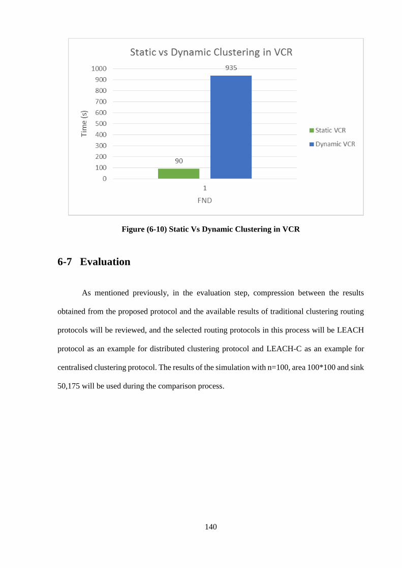
140
Figure (6-10) Static Vs Dynamic Clustering in VCR
6-7 Evaluation
As mentioned previously, in the evaluation step, compression between the results
obtained from the proposed protocol and the available results of traditional clustering routing
protocols will be reviewed, and the selected routing protocols in this process will be LEACH
protocol as an example for distributed clustering protocol and LEACH-C as an example for
centralised clustering protocol. The results of the simulation with n=100, area 100*100 and sink
50,175 will be used during the comparison process.

141
6-7-1 Experiment Six: Lifetime measurement based on First Node Dead
(FND)
As described in chapter two, the network lifetime in WSN can be defined as the time
duration between the start of the communication process and first, half or last dead sensor
nodes. In this thesis, the First Node Dead (FND) will be used to represent the network lifetime.
The important difference between the proposed protocol, LEACH and LEACH-C is the
round timeline, and the round time depends on a pre-define time value, which has been defined
by the researchers. Also, the number of cycle is not fixed and depends on a specific time as
well.
For LEACH-C, the sending process for the nodes information at the beginning of each
round adds an extra overhead for the nodes. However, in this thesis, and as mentioned
previously, the cluster head selection process depends on a certain energy threshold, and the
number of a cycle of the round depends on the number of clusters in the network, and the
checking process occurs at the end of each cycle.
The cluster management during the protocol operation is separated, which means the
behaviour of the clusters is not fixed and depends on the number of nodes within the clusters.
This scheme will manage the time for nodes to become cluster heads and thus, will affect the
lifetime of the node.
Furthermore, by moving the setup stage into the smart environment (NFV server in
cloud system), this will lead to minimising the amount of communication required for this stage
and prevent the nodes from sending their information each time at the beginning of each round.
All these factors affect the network lifetime, as shown in Figure (6-11) that illustrates the
comparison between the VCR, LEACH and LEACH-C in terms of FND.

142
Figure (6-11) Comparison among Proposed Protocol, LEACH and LEACH-C
From this bar chart, the proposed protocol has outperformed LEACH and LEACH-C by
doubling the network lifetime; this is considered a significant improvement in the network
because of the new protocol minimising the overhead of the cluster formation and cluster head
selection.
6-7-2 Experiment Seven: Start-up Cost
In LEACH, the cost of the startup stage contains various messages exchanged in order
to start building the clusters such as cluster head’s advertisement, the joining request message
from the normal node and the time slot for each cluster member. On the other hand, for LEACH-
C, the startup step has more energy consumption than the LEACH because of the transmission
process for nodes information to the sink that occurs at the beginning of each round.
At the beginning of the proposed protocol process, and as mentioned previously, the
senor nodes will send a short message to communicate its location and energy level to the base

143
station that in turn will forward it to the NFV server. This message will be sent once and does
not need to be sent again because of the utilities of the smart environment provided by the cloud
application (NFV server). According to this, the total energy consumption in this stage for the
proposed protocol, LEACH and LEACH-C, is shown in Figure (6-12).
Figure (6-12) Startup Energy Consumption
From this figure, the startup cost in the proposed protocol is high at the beginning of the
stage when the nodes transmit their information to the sink, but after that, the consumption is
minimised and stable because the node consumes its energy in the same procedure, which
receives the clustering information from the server via the sink.
On the other hand, in LEACH, the amount of energy in the startup stage is different in
each round because the number of nodes that will be a cluster head is different and thus will
affect the amount of energy consumption.
144
By comparing between the proposed protocol and LEACH, it is obvious that the new
protocol consumes more energy than LEACH just at the beginning of the first round and it will
be superior to the rest of the protocol operation because of the minimising of the number of
communications.
For LEACH-C, the start-up energy consumption is fixed because of the same procedure
happening at each round (same transmission process, as the node, sends its information to the
sink at the beginning of every new round).
6-7-3 Experiment Eight: CH role Rotation
As mentioned previously, the rotation time for the node to be a cluster head is important
to balance nodes’ energy consumption. In other words, if the rotation time is fixed, too small
or too long, the energy consumption distribution will be unbalanced among the node. Also,
checking the node energy at each cycle is important to monitor the network and manage the
nodes.
Some clustering based protocols use static clustering, which means as soon as the cluster
forms and the cluster head selected, the clusters will be fixed. In spite of this process removes
the overhead of the setup stage, but also makes the clusters depend on just one node as a cluster
head, and this node will consume all its energy at a fast pace to make the whole cluster isolated
from the network and dead.
Figure (6-13) represents the behaviour of the proposed protocol and LEACH protocol
for static clustering. It shows that in spite of the static clustering being inefficient for the
network lifetime, the behaviour of the proposed protocol is better than the LEACH and
duplicates the network lifetime. By using the cloud based technique and static clustering (re-
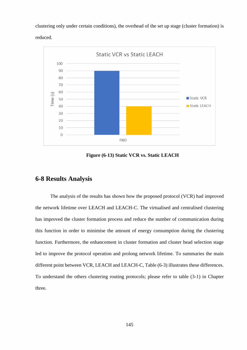
145
clustering only under certain conditions), the overhead of the set up stage (cluster formation) is
reduced.
Figure (6-13) Static VCR vs. Static LEACH
6-8 Results Analysis
The analysis of the results has shown how the proposed protocol (VCR) had improved
the network lifetime over LEACH and LEACH-C. The virtualised and centralised clustering
has improved the cluster formation process and reduce the number of communication during
this function in order to minimise the amount of energy consumption during the clustering
function. Furthermore, the enhancement in cluster formation and cluster head selection stage
led to improve the protocol operation and prolong network lifetime. To summaries the main
different point between VCR, LEACH and LEACH-C, Table (6-3) illustrates these differences.
To understand the others clustering routing protocols; please refer to table (3-1) in Chapter
three.
146
6-9 Summary
In this chapter, proposed protocol has been implemented, validated and evaluated. The
behaviour of the network was tested based on various scenarios and parameters such as a
various number of nodes, different sink position as well as different area size in order to validate
the operation of protocol. In addition, the optimum number of clusters was found with various
numbers of nodes and verified the results from the optimum number of clusters equation.
For the evaluation, the results showed that the VCR is better than the LEACH and
LEACH-C protocols in terms of first node dead (FND) and the network lifetime was improved
and doubled.

147
Protocol Classification Basic definition Advantage Disadvantage
LEACH Distributed - The first protocol in
distributed clustering
based approach.
- The cluster head role is
distributed among the
nodes.
- The clustering approach is
based on a random process.
- Cluster heads are selected
first, then, the cluster will
be formed (nodes join the
nearest cluster head).
- Better than flat protocols in
improving the network’s
performance.
- The number of clusters are
changeable for each round
- The random clustering results
in an even distribution of CH
role among the nodes.
- The clusters may not cover the
whole network.
- Not suitable in mobile networks
- There is no guarantee to
produce an optimum number of
clusters because of the random
process.
- The round rotation is based on
time (does not take into account
the energy level of the nodes).
LEACH-C Centralised (Sink is
responsible for the
clustering function
- The first protocol in
Centralised clustering based
approach.
- Centralised version of
LEACH to improve the
network performance and
lifetime.
- A list of cluster head will be
generated based on nodes
energy level and will be fixed
during the protocol operation.
- Cluster heads selected first,
then, the cluster will be
- Centralised responsibility
by the sink improves
network management and
control
- LEACH-C improves the
packets delivery of LEACH
by 40%
- Generate a list of CHs nodes,
which is unchangeable.
- Not suitable in mobile
networks.
- The round rotation is based on
time (do not take into account
energy level of the nodes).
Table (6-3) Comparison among LEACH, LEACH-C and VCR

148
formed (nodes join the
nearest cluster head).
VCR Virtualised and
Centralised
(the server is
responsible for the
clustering
function)
- Clusters formed first,
after that the cluster heads
will be selected
- Clusters formed first
based on a clustering
algorithm (k-means), after
that the cluster heads
would be selected.
- Cluster head selection is
based on a cost function
that combines the nodes’
distance to the sink and
their energy level (this cost
function is updated at the
end of each cycle)
- The round rotation is
based on a certain
condition (using the nodes’
current energy level)
- The optimum number of
clusters is found by the
central server to improve
network management.
- Use nodes energy level,
distance to sink and distance
among nodes for effeicint
clustering fucntion.
- By comparing it with
LEACH and LEACH-C , the
network lifetime had been
enhanced to double.
- Not suitable in mobile
networks

149
Chapter Seven
Conclusions and Future works
7-1 Introduction
In this thesis, a new virtualised and centralised routing protocol has been proposed to
enhance the network lifetime and minimise the amount of energy consumption that is required
to the clustering function in clustering sensor networks. The new protocol utilises the approach
of the cloud computing and enables a NFV server to manage and control the network. This
chapter introduces the conclusions as well as the future works required of this research.
7-2 Conclusions
Improving the network lifetime and minimise the energy consumption for the sensor
nodes were the aim of this thesis. The new protocol represents a design that combines the
concept of the network function virtualisation as an application of cloud computing and the
smart environment by moving and virtualising a clustering function to be operated on a central
server. Using the server concept makes the function sharable and able to be utilised by any
WSN. The results show that the new protocol outperforms the existing cluster protocols and
network lifetime has been doubled.
In conclusions, and based on the results, using a central server to manage and control
the network is efficient to minimised the number and the amount of communications as well as
use efficient clustering function will led to balance the energy consumption among the nodes
and improve network lifetime.

150
The objective of this thesis were achieved and will now be summarised in the following
paragraphs. Chapter one contained a brief introduction to the system design as well as the main
research problem, which refers to the energy consumption in WSN generally and in clustering
function precisely. The aim, objectives, hypothesis and contribution of the research were
explained and reviewed, and finally, the general steps of the methodology used during this
research were included. Furthermore, a simple definition of NFV was also presented in this
chapter because of the NFV is the important part of this research.
Moreover, in order to understand the concept of WSN, a full information and
background for what WSN means, main components, applications types and the energy
consumptions fields and how it can be minimised were outlined in Chapter Two. The
characteristics and classifications of the routing protocols were also reviewed, and these
reviews helped to identify the various problems in the design of this type of network and find
out the main points that should be taken into account during the design of any routing protocols.
To clarify the general concepts clustering functions and the energy consumption
problem in the clustering function, a comprehensive literature review was provided in Chapter
Three; besides this, the main clustering routing protocols classification of distributed and
centralised routing protocols and their types were discussed. As a case study, the details and
behaviours of the first clustering protocol (LEACH) were explained.
Various methods can be used to extend network lifetime and reduce the power
consumption of the sensor nodes. One of these methods is the reduction in the number of
transmitted and received control messages and minimising the computation needed for each
node during the stages of cluster formation and cluster head selection. In this thesis, a new
clustering based routing protocol known Virtualised Clustering Routing (VCR) Protocol has
been introduced. The VCR reduced the number of communications between nodes and

151
minimised the computation overhead in each node. Full details and characteristics of this new
protocol were described in Chapter Four. The new protocol uses NFV principles to virtualise
the clustering function and move it to a centralised server with considerably higher processing
capabilities. This technique produce more energy efficient clustering and allows the server to
apply machine-learning techniques (k-means) to the clustering function, which is based on the
square distance among the nodes; this achieves the clustering in the best shape with minimum
distance among nodes.
Furthermore, as mentioned in the description of k-means algorithm, the final clusters
formed after certain convergence iterations, that cannot be random or constant. Therefore, in
order to find these convergence iterations, k-means have been simulated for various testes,
which based on different number of nodes in the network and various network topologies.
Furthermore, by combining the distance to sink and current energy level, this achieves
the best selection for the cluster head. Also, the duration of the node to be a cluster head is
necessary to guarantee the energy consumption distributed among the nodes and prolong
network lifetime.
Then, as mentioned previously, the energy level of the node will be monitored and
estimated by the server, this will be done by the proposed analytical model that was introduced
in Chapter Five. This model takes into consideration the various fields in which the nodes
consumed their energy and modified it according to the proposed protocol operation.
Furthermore, to illustrate the number of communications in the LEACH protocol, a
mathematical model for LEACH was derived and explained in this chapter. The purpose of this
model to make a compression with the proposed protocol in terms of numbers of
communications during the clustering function.
152
The simulation and tested scenarios for the protocol were introduced in Chapter Six.
The protocol was tested based on various scenarios such as changing a number of nodes in the
network, changing the sink position as well as modifying the size of the coverage area.
Moreover, the most important issue is a centralised protocol to find the optimum number of
clusters to enhance the protocol performance. Therefore, this value was determined based on
different scenarios as described in this Chapter.
The validation showed that the behaviour of the protocol is variable and depends on
various parameters such as nodes density, sink position as well as the sensing area size. The
results showed that the amount of energy consumption is increased when the sink is located
outside the sensing area and the sensing area size is maximised because the energy consumption
depends on the distance between the nodes within the clusters and between the cluster heads
and the sink.
For the evaluation, LEACH and LEACH-C were used to evaluate the design in dynamic
and static environment. The selection of these protocols were done because they represent the
first and popular protocols in distributed and centralised clustering and they were the base for
most of the available clustering protocols.
The evaluation was based on a comparison among the VCR protocol, the LEACH and
the LEACH-C with different criteria such as First Node Dead (FND) and start-up cost. It can
be concluded that a significant reduction in the communication cost was achieved and thus,
affects the network lifetime. The results regarding First Node Dead (FND) showed that the new
protocol outperforms the LEACH and LEACH-C and the network lifetime was doubled.
7-4 Future Works
The following ideas could be used as a future development of this research:

153
1- Implement the design in real environment in order to study the protocol operations in
this field.
2- As the style of intra and inter communications were based on single-hop, the sensor
nodes consumed a significant amount of energy during the protocol operation when the
size of the network was increased. Therefore, the protocol should be tested by changing
the communication style to be in the multi-hop scheme for either intra or inter
communication or both and find how the system will perform in larger network sizes.
3- In some WSN applications, the mobility of nodes is necessary to perform tracking or
monitoring tasks. Therefore, the mobility of the sensor nodes during the protocol
operation can be adopted in future work.
4- The implementation is based on a single sink as a data gathering point. In a future work,
multi-sinks could be included to distribute and balance the energy consumption and
investigate the network behaviour. In addition, make the sink responsible on the starting
of the operation.
154
Publications
The following is the list of the publications produced during the development of this research.
1- R. Al-Nuaimi and A.Al-Yasiri, “ENERGY EFFICIENT ROUTING IN WSN BASED
ON VIRTUALIZATION”, College Dean’s Annual Research Showcase Event,
University Of Salford, UK, 2014.
2- R. Al-Nuaimi and A.Al-Yasiri, “A NEW ENERGY-EFFICIENT CLUSTERING
ALGORITHM FOR WIRELESS SENSOR NETWORKS BASED ON NETWORK
FUNCTION VIRTUALISATION (NFV) AND THE LEACH ROUTING
PROTOCOL”, College Dean’s Annual Research Showcase Event, University Of
Salford, UK, 2015.
3- R. Al-Nuaimi and A.Al-Yasiri, “A NEW ENERGY-EFFICIENT CLUSTERING
PROTOCOL FOR WIRELESS SENSOR NETWORKS BASED ON NETWORK
FUNCTION VIRTUALISATION (NFV)”, The 6th International Conference on
Information Communication and Management(ICICM 2016), IEEE Conference, UK,
2016.

155
References
Abbas, A. A., & Younis, M. (2007). A survey on clustering algorithms for wireless sensor
networks. Computer communications, 30(14-15), 2826-2841.
doi:10.1016/j.comcom.2007.05.024
Abidi, B., Jilbab, A., & Haziti, M. E. (2017). Wireless Sensor Networks in Biomedical:
Wireless Body Area Networks Europe and MENA Cooperation Advances in
Information and Communication Technologies (pp. 321-329): Springer.
Adinya, O. J., & Daoliang, L. (2013). Transceiver Energy Consumption Models for the Design
of Low Power Wireless Sensor Networks. Odey John Adinya et al | IJCSET, 3(4).
Ahmedy, I., Ngadi, M. A., Omar, S. N., & Chaudhry, J. (2011). A review on wireless sensor
networks routing protocol: Challenge in energy perspective. Scientific Research and
Essays, 6(26). doi:10.5897/sre11.640
Akkaya, K., & Younis, M. (2003). A Survey on Routing Protocols for Wireless Sensor
Networks. Ad hoc networks, 3(3), 325-349.
Akyildiz, Su, Sankarasubramaniam, & Cayirci. (2002a). Wireless sensor networks: a survey.
IEEE communications magazine, 40(8), 102-114.
Akyildiz, Su, Sankarasubramaniam, & Cayirci. (2002b). Wireless sensor networks: a survey.
Computer Networks 38, 38, 393–422.
Al-Karaki, J. N., & Kamal, A. E. (2004). Routing Techniques in Wireless Sensor Networks: A
Survey. IEEE wireless communications, 11(6), 6-28.
Al-Karaki, J. N., & Kamal, A. E. (2005). A Taxonomy of Routing Techniques in Wireless
Sensor Networks Handbook of Sensor Networks: Compact Wireless and Wired Sensing
systems.

156
Al-Obaisat, Y., & Braun, R. (2007). On wireless sensor networks: architectures, protocols,
applications, and management.
Ali, S. J., & Roy, P. (2008). Energy Saving Methods in Wireless Sensor Networks (Based on
802.15.4). (degree of Master), Halmstad University, Högskolan i Halmstad/Sektionen
för Informationsvetenskap, Data- och Elektroteknik (IDE).
Alkhatib, A. A. A., & Baicher, G. S. (2012). Wireless Sensor Network Architecture. The
International Conference on Computer Networks and Communication Systems (CNCS
2012). Singapore.
Amini, N., Vahdatpour, A., Xu, W., Gerla, M., & Sarrafzadeh, M. (2012). Cluster Size
Optimization in Sensor Networks with Decentralized Cluster-Based Protocols.
Computer communications, 35(2), 207-220.
Anastasi, G., Conti, M., Di Francesco, M., & Passarella, A. (2009). Energy conservation in
wireless sensor networks: A survey. Ad hoc networks, 7(3), 537-568.
doi:10.1016/j.adhoc.2008.06.003
Anastasi, G., Francesco, M. D., Conti, M., & Passarella, A. (2006). How to prolong the lifetime
of wireless sensor networks (pp. 1-26): Valencia, CA: American Scientific Publishers.
Arboleda, L., & Nasser, N. (2006). Comparison Of Clustering Algorithms And Protocols For
Wireless Sensor Networks. The Electrical and Computer Engineering CCECE'06,
Canadian Conference.
Arumugam, G. S., & Ponnuchamy, T. (2015). EE-LEACH: development of energy-efficient
LEACH Protocol for data gathering in WSN. EURASIP Journal on Wireless
Communications and Networking, 2015(1), 1-9.
Aslam, M., Javaid, N., Rahim, A., Nazir, U., Bibi, A., & Khan, Z. A. (2012). Survey of
Extended LEACH-Based Clustering Routing Protocols for Wireless Sensor Networks.
157
The High Performance Computing and Communication & 2012 IEEE 9th International
Conference on Embedded Software and Systems (HPCC-ICESS), Liverpool, UK.
Aslam, M., Rasheed, M. B., T. Shah, A. R., Khan, Z. A., Qasim, U., Qasim, M. W., . . . Javaid,
N. (2013). Energy optimization and Performance Analysis of Cluster Based Routing
Protocols Extended from LEACH for WSNs. arXiv preprint arXiv, 1309.4373.
Ayyat, S. (2013). DIFFSENSE-A Qualityof Service Architecture for Wireless Sensor Networks
Based on Traffic Classification. (P.hD), University of Salford, University of Salford.
Bhakti Parmar, J. M., Jemish Meisuria, Ajay Singh. (2014). A Survey of routing protocol
LEACH for WSN. International Journal of Scientific and Research Publications, 4(1).
Biradar, Patil, Sawant, & Mudholkar. (2009). Classification And Comparison Of Routing
Protocols In Wireless Sensor Networks. Special Issue on Ubiquitous Computing
Security Systems, 4(2), 704-711.
Bora, D. J., & Gupta, D. A. K. (2014). A Comparative study Between Fuzzy Clustering
Algorithm and Hard Clustering Algorithm. International Journal of Computer Trends
and Technology (IJCTT), 10(2).
Buratti, C., Conti, A., Dardari, D., & Verdone, R. (2009). An overview on wireless sensor
networks technology and evolution. Sensors, 9(9), 6869-6896. doi:10.3390/s90906869
Cecílio, J., Anjos, E., Costa, J., & Furtado, P. (2010). SURVEY ON DATA ROUTING IN
WSN. Wireless Sensor Network Technologies for the Information Explosion Era, 3-46.
Central, S. (2013). What’s NFV – Network Functions Virtualization. From
www.sdncentral.com/whats-network-functions-virtualization-nfv/
Chen, G., Li, C., Ye, M., & Wu, J. (2007). An unequal cluster-based routing protocol in wireless
sensor networks Wireless Networks (Vol. 15, pp. 193-207): Springer US.
Chen, J., Li, Z., & Kuo, Y.-H. (2013). A centralized balance clustering routing protocol for
wireless sensor network. Wireless personal communications, 72(1), 623-634.

158
corporation, C. (2013). Cloud NFV units , the best of NFV , cloud computing and SDN.
Dargie, W., & Poellabauer, C. (2010). Fundamentals Of Wireless Sensor Networks. United
Kingdom: A John Wiley and Sons, Ltd., Publication.
Dekivadiya, D., & Vadharia, V. (2012). Performance Analysis of Routing Protocols of Wireless
Sensor Networks. (Bachelor of Technology In Computer Engineering).
Devi, R. R., & Sethukkarasi, R. (2016). A Study on Classification of Energy Efficient Routing
Protocols in Wireless Sensor Networks. International Journal of Innovative Research
and Development|| ISSN 2278–0211, 5(4).
Enam, R. N., Imam, M., & Qureshi, R. I. (2012). Energy Consumption in Random Cluster Head
selection Phase of WSN. The International Proceedings of Computer Science &
Information Tech IPCSIT 30 Singapore.
Eslaminejad, M., & Razak, S. A. (2012). Fundamental lifetime mechanisms in routing protocols
for wireless sensor networks: a survey and open issues. Sensors (Basel), 12(10), 13508-
13544. doi:10.3390/s121013508
ETSI. (2012). Netwrok Function Virtulization_Introductory white paper. The SDN and
Openflow world Congress, Germany.
ETSI. (2013a). Network Functions Virtualisation (NFV). The SDN and OpenFlow World
Congress, Frankfurt-Germany. http://portal.etsi.org/NFV/NFV_White_Paper2.pdf
ETSI. (2013b). Netwrok Function Virtulization_Updated white paper. The SDN and Openflow
world Congress.
Gawade, R. D., & Nalbalwar, S. (2016). A centralized energy efficient distance based routing
protocol for wireless sensor networks. Journal of Sensors.
Gowrishankar, Basavaraju, Manjaiah, & Sarkar, S. K. (2008). Issues in Wireless Sensor
Networks. The World Congress on Engineering 2008, London, U.K.

159
Gupta, S. K., Jain, N., & Sinha, P. (2013). Clustering Protocols in Wireless Sensor Networks:
A Survey. International Journal of Applied Information Systems (IJAIS), 5(2).
Han, B., Zhang, D., & Yang, T. (2008). Energy Consumption Analysis and Energy
Management Strategy for Sensor Node. The Proceedings of the 2008 IEEE
International Conference on Information and Automation, China.
Hani, R. M. B., & Ijjeh, A. A. (2013). A Survey on LEACH-Based Energy Aware Protocols
for Wireless Sensor Networks. Journal of Communications, 8(3), 192-206.
doi:10.12720/jcm.8.3.192-206
Hatamian, M., Barati, H., Movaghar, A., & Naghizadeh, A. (2016). CGC: centralized genetic-
based clustering protocol for wireless sensor networks using onion approach.
Telecommunication Systems, 62(4), 657-674.
Heinzelman, Chandrakasan, A., & Balakrishnan, H. (2000). Energy-Efficient Communication
Protocol forWireless Microsensor Networks. The 33rd Hawaii International
Conference on System Sciences, Hawaii.
Heinzelman, W. B. (2002). Application Specifc Protocol Architectures for Wireless Networks.
(PhD), Massachusetts Institute Of Technology.
Heinzelman, W. B., Chandrakasan, A. P., & Balakrishnan, H. (2002). An Application-Specific
Protocol Architecture for Wireless Microsensor Networks. IEEE Transactions on
Wireless Communications, 1(4).
Hou, G., Tang, K. W., & Noel, E. (2013). Implementation and Analysis of the LEACH Protocol
on the TinyOS Platform. The International Conference on ICT Convergence (ICTC).
Hu, F., & Cao, X. (2010). Wireless Sensor Networks: Principles and Practice: CRC Press.
Iqbal, A., Akbar, M., Javaid, N., Bouk, S. H., Ilahi, M., & Khan, R. D. (2013). Advanced
LEACH: A Static Clustering-based Heteroneous Routing Protocol for WSNs. arXiv
preprint arXiv, 1306.1146.
160
Jain, R. (2013). Introduction to Network Function Virtualization (NFV). From Washington
University in Saint Louis: http://www.cse.wustl.edu/~jain/cse570-13/
Jun, W., Xin, Z., Junyuan, X., & Zhengkun, M. (2010). A Distance-based Clustering Routing
Protocol in Wireless Sensor Networks. The Communication Technology (ICCT), 2010
12th IEEE International Conference.
Kalantary, S., & Taghipour, S. (2014). A survey on architectures, protocols, applications, and
management in wireless sensor networks. Journal of Advanced Computer Science &
Technology, 3(1). doi:10.14419/jacst.v3i1.1583
Kaur, A., & Grover, A. (2015). LEACH and Extended LEACH Protocols in Wireless Sensor
Network-A Survey. International Journal of Computer Applications, 116(10).
Khurana, N. (2013). ROUTING ALGORITHMS IN WSN : A SURVEY. VSRD International
Journal of Computer Science & Information Technology, 3(2).
Kumar, A., & Singh, D. (2016). Importance Of Energy In Wireless Sensor Networks: A Survey.
An International Journal of Engineering Sciences, 17, 500-505.
Kumar, V., Dhok, S. B., Tripathi, R., & Tiwari, S. (2014). A Review Study on Analytical
Estimation of Optimal Number of Clusters in Wireless Sensor Networks. transactions
on networks and communication s, 2(5).
Kumarawadu, P., Dechene, D. J., Luccini, M., & Sauer, A. (2008). Algorithms for Node
Clustering in Wireless Sensor Networks: A Survey. the Information and Automation for
Sustainability, 2008. ICIAFS 2008. 4th International Conference on.
lal Parmar, A. M., & Thakkar, A. (2016). An improved modified LEACH-C algorithm for
energy efficient routing in Wireless Sensor Networks. Nirma University Journal of
Engineering and Technology, 4(2), 1-5.
Leskovec, J., Rajaraman, A., & Ullman, J. D. (2014). Mining of Massive Datasets.
161
Lewis, Moncrief-O’Donnell, & Chair, E. (2006). Wireless Sensor Networks: Issues, Advances,
and Tools. The University of Texas at Arlington. Retrieved from
http://www.uta.edu/utari/acs/FL%20talks/WSN%20NTU%2006.pdf
Li, H., & Liu, J. (2016). Double cluster based energy efficient routing protocol for wireless
sensor network. International Journal of Wireless Information Networks, 23(1), 40-48.
Lindsey, S., & Raghavendra, C. S. (2002). PEGASIS: Power-efficient gathering in sensor
information systems. The Aerospace conference proceedings.
Liu, F., Tsui, C.-Y., & Zhang, Y. J. (2010). Joint routing and sleep scheduling for lifetime
maximization of wireless sensor networks. IEEE Transactions on Wireless
Communications, 9(7), 2258-2267.
Liu, X. (2012). A survey on clustering routing protocols in wireless sensor networks. Sensors
(Basel), 12(8), 11113-11153. doi:10.3390/s120811113
Loscri, V., Morabito, G., & Marano, S. (2005). A two-levels hierarchy for low-energy adaptive
clustering hierarchy (TL-LEACH). The 62nd IEEE vehicular technology conference.
MacQueen, J. (1967). Some methods for classification and analysis of multivariate
observations. The fifth Berkeley symposium on mathematical statistics and probability.
Madan, R., & Lall, S. (2006). Distributed Algorithms for Maximum Lifetime Routing in
Wireless Sensor Networks. IEEE Transactions on Wireless Communications, 5(8), 6-
28.
Mahboub, A., Arioua, M., & Ez-Zazi, I. (2016). Performance Evalution Of Energy-Efficient
Clustering Algorithms In Wireless Sensor Networks. Journal of Theoretical and
Applied Information Technology, 83(2), 187.
Malfa, S. L. (2010). A Sensing Architecture for Mutual User-Environment Awareness Case of
Study: A Mobility Aid for the Visually Impaired. IEEE Sensors Journal, 11(3), 634 -
640. doi:10.1109/JSEN.2010.2053843
162
Manjeshwar, A., & Agrawal, D. P. (2001). TEEN: a routing protocol for enhanced efficiency
in wireless sensor networks. The Parallel and Distributed Processing Symposium,
International.
Manjeshwar, A., & Agrawal, D. P. (2002). APTEEN: A Hybrid Protocol for Efficient Routing
and Comprehensive Information Retrieval in Wireless Sensor Networks. The
International Parallel and Distributed Processing Symposium (IPDPSí02)
Mir, N. F. (2014). Computer and communication networks: Pearson Education.
Mundada, M. R. (2012). A Study On Energy Efficient Routing Protocols In Wireless Sensor
Networks. International Journal of Distributed and Parallel systems, 3(3), 311-330.
doi:10.5121/ijdps.2012.3326
Muruganathan, S. D., Ma, D. C. F., Bhasin, R. I., & Fapojuwo, A. O. (2005 ). A Centralized
Energy-Efficient Routing Protocol for Wireless Sensor Networks. IEEE
communications magazine, 43(3), S8-13.
Pakzad, S. N., Fenves, G. L., Kim, S., & Culler, D. E. (2008). Design and Implementation of
Scalable Wireless Sensor Network for Structural Monitoring. Journal Of Infrastructure
Systems.
Pal, A. (2010). Localization Algorithms in Wireless Sensor Networks: Current Approaches and
Future Challenges. Network Protocols and Algorithms, 2(1), 45-73.
Pal, V., Singh, G., Yadav, & Pal, P. (2012). Energy Efficient Clustering Scheme for Wireless
Sensor Networks: A Survey. Journal of Wireless Networking and Communications 2(6),
168-174 /doi:10.5923/j.jwnc.20120206.02.
Pantazis, N. A., Nikolidakis, S. A., & Vergados, D. D. (2013). Energy-Efficient Routing
Protocols in Wireless Sensor Networks: A Survey. IEEE Communications Surveys &
Tutorials, 15(2).

163
Pantazis, N. A., Vergados, D. J., Vergados, D. D., & Douligeris, C. (2009). Energy efficiency
in wireless sensor networks using sleep mode TDMA scheduling. Ad hoc networks,
7(2), 322-343. doi:10.1016/j.adhoc.2008.03.006
Pare, A., & Dongre, A. (2015). Analysis Of Wireless Sensor Network Protocol. IJAICT 1 (11).
Parvin, S., & Rahim, M. S. (2008). Routing Protocols for Wireless Sensor Networks: A
Comparative Study. The International Conference on Electronics, Computer and
Communication (ICECC 2008), University of Rajshahi, Bangladesh.
Pate, P. (2013). NFV and SDN: What’s the Difference? from
www.sdncentral.com/technology/nfv-and-sdn-whats-the-difference/2013/03/
Patil, & Patil, A. J. (2013). An Efficient Power Saving Mechanism Issues for Wireless Sensor
Networks. International Journal of Software and Web Sciences (IJSWS).
Patil, P., Kulkarni, U., & Ayachit, N. H. (2011). Some Issues in Clustering Algorithms for
Wireless Sensor Networks. IJCA Special Issue on “2nd National Conference-
Computing, Communication and Sensor Network” CCSN.
Pawa, T. D. S. (2011). Analysis of Low Energy Adaptive Clustering Hierarchy (LEACH)
protocol. (Bachelor of Technology), National Institute of Technology Rourkela.
Potdar, V., Sharif, A., & Chang, E. (2009). Wireless Sensor Networks: A Survey. 636-641.
doi:10.1109/waina.2009.192
Pottie, G. J., & Kaiser, W. J. (2000). Wireless integrated network sensors. Commun. ACM,
43(5), 51-58. doi:10.1145/332833.332838
Radcom. (2013). Network Analytics Probes in the NFV and SDN Era.
Rahman, M. M., Miah, M. S., & Sharmin, D. (2016). Cognitive Improved LEACH
(CogILEACH) Protocol for Wireless Sensor Network. Transactions on Networks and
Communications, 4(6), 01.

164
Rajaravivarma, V., Yang, Y., & Yang, T. (2003). An overview of wireless sensor network and
applications. Paper presented at the System Theory, 2003. Proceedings of the 35th
Southeastern Symposium on.
Ramesh, & Somasundaram. (2011). A Comparative Study Of Clusterhead Selection Algorithms
In Wireless Sensor Networks. International Journal of Computer Science &
Engineering Survey, 2(4), 153-164. doi:10.5121/ijcses.2011.2411
Ramya, R., Saravanakumar, G., & Ravi, S. (2016). Energy Harvesting in Wireless Sensor
Networks Artificial Intelligence and Evolutionary Computations in Engineering
Systems (pp. 841-853): Springer.
Razaque, A., Abdulgader, M., Joshi, C., Amsaad, F., & Chauhan, M. (2016). P-LEACH: Energy
efficient routing protocol for Wireless Sensor Networks. The Long Island Systems,
Applications and Technology Conference (LISAT), 2016 IEEE.
Rezaei, Z., & Mobininejad, S. (2012). Energy Saving in Wireless Sensor Networks.
International Journal of Computer Science & Engineering Survey, 3(1), 23-37.
doi:10.5121/ijcses.2012.3103
Sabor, N., Sasaki, S., Abo-Zahhad, M., & Ahmed, S. M. (2017). A Comprehensive Survey on
Hierarchical-Based Routing Protocols for Mobile Wireless Sensor Networks: Review,
Taxonomy, and Future Directions. Wireless Communications and Mobile Computing,
2017.
Sadhana, Malik, T., Gogia, R., Devi, S., & Chhabra, P. (2013). Virtual Wireless Sensor
Networks. International Journal Of Technological Exploration And Learning (Ijtel),
2(6).
Sahni, S., & Xu, X. (2004). Algorithms For Wireless Sensor Networks. International journal
of distributed sensor networks, 1(1), 35-56.

165
Sendra, S., Lloret, J., García, M., & Toledo, J. F. (2011). Power saving and energy optimization
techniques for Wireless Sensor Networks. Journal Of Communications, 6(6).
Shaikh, F. K., & Zeadally, S. (2016). Energy harvesting in wireless sensor networks: A
comprehensive review. Renewable and Sustainable Energy Reviews, 55, 1041-1054.
Sharma, A., Shinghal, K., Srivastava, N., & Singh, R. (2011). Energy Management for Wireless
Sensor Network Nodes. International Journal of Advances in Engineering &
Technology, 1.
Sharma, G. (2009). Routing In Wireless Sensor Networks. (Master of Engineering in Computer
Science & Engineering), Thapar University.
Sheth, S., & Rathod, H. (2015). Comparative Study of Variants of Low Energy Adaptive
Clustering Hierarchy (LEACH) Protocol in Wireless Sensor Networks. International
Journal for Scientific Research & Development|, 2(11).
Shigei, N., Miyajima, H., & Morishita, H. (2010). Energy consumption reduction of clustering
communication based on number of neighbors for wireless sensor networks.
International Journal of Computer Science, 37(3), 3-11.
Singh, & Arora, H. (2013). Design and Architectural Issues in Wireless Sensor Networks.
International Journal of Advanced Research in Computer Science and Software
Engineering, 3(1).
Singh, & Sharma, S. C. (2014). Cluster Based Routing Algorithms for Wireless Sensor
Networks. IJETI International Journal of Engineering & Technology Innovations,
11(4).
Singh, & Sharma, S. C. (2015). A Survey on Cluster Based Routing Protocols in Wireless
Sensor Networks. The International Conference on advanced Computing technologies
and Applications (ICACTA-2015).

166
Singh, C., & Aloney, M. R. (2015). Comparative Study of LEACH Routing Protocol for WSN.
International Journal of Advance Research in Computer Science and Management
Studies, 3(3).
Singh, S. K., Singh, M. P., & Singh, D. K. (2010). Routing Protocols in Wireless Sensor
Networks - A Survey. International Journal of Computer Science & Engineering
Survey, 1(2), 63-83. doi:10.5121/ijcses.2010.1206
Srivastava, M. (2002). Sensor node platforms and energy issues. The Proceedings of the 8th
ACM International Conference on Mobile Computing and Networking (MobiCom’02),
Atlanta, GA.
Sumathi, R., & Srinivas, M. G. (2012). A Survey of QoS Based Routing Protocols for Wireless
Sensor Networks. Journal of Information Processing Systems, 8(4), 589-602.
doi:10.3745/jips.2012.8.4.589
Tan, H.-X. (2006). Quality of Service in Wireless Sensor Networks. Retrieved from Final Report
in CS6204-AY05/06 Semester II:
Taylor, M., CTO, & Networks, M. (2014). A Guide to NFV and SDN.
Thakkar, A. (2016). Cluster head election techniques for energy-efficient routing in Wireless
Sensor Networks-An updated survey. IAENG International Journal of Computer
Science, 7(2), 218-245. doi:10.090592/IJCSC.2016.135
Thangadurai, N., & Dhanasekaran, R. (2013). Optimal Energy Consumption to Extend the
Lifetime of Wireless Sensor Networks. Journal of Computer Science, 9(5), 646-653.
doi:10.3844/jcssp.2013.646.653
Tian, D., & Georganas, N. D. (2002). A coverage-preserving node scheduling scheme for large
wireless sensor networks. The Proceedings of the 1st ACM international workshop on
Wireless sensor networks and applications.
167
Tiwari, A. (2016). Energy Efficient Protocol for Multilevel Clustering Reducing the Energy
Consumption of WSN. IJSRSET, 2(1), 390-393.
Tong, M., & Tang, M. (2010). LEACH-B:An Improved LEACH Protocol for Wireless Sensor
Network. The 6th International Conference on Wireless Communications Networking
and Mobile Computing (WiCOM). IEEE.
Tripathy, A. K., & Chinara, S. (2012). Comparison of residual energy-based clustering
algorithms for wireless sensor network. ISRN Sensor Networks, 2012.
Upadhyay, V., & Swaroop, A. (2016). A survey of LEACH based routing protocols for WSN.
School of Computer Science and Engineering, Galgotias University, Greater Noida,
India, 3.
Vashist, S., & Khurana, J. (2013). Enhanced Leach Protocol to Increase Network Life Time.
International Journal of Emerging Technology and Advanced Engineering, 3(6).
Villalba, L. J., Orozco, A. L., Cabrera, A. T., & Abbas, C. J. (2009). Routing protocols in
wireless sensor networks. Sensors (Basel), 9(11), 8399-8421. doi:10.3390/s91108399
Voigt, T., Dunkels, A., Alonso, J., Ritter, H., & Schiller, J. (2004). Solar-aware Clustering
inkwireless Sensor Networks. The Proceedings. ISCC 2004. Ninth International
Symposium on Computers And Communications (IEEE Cat. No.04TH8769).
Wikibon. (2013). Network Function Virtualization or NFV Explained. from
wikibon.org/wiki/v/Network_Function_Virtualization_or_NFV_Explained
Xiangning, F., & Yulin, S. (2007). Improvement on LEACH protocol of wireless sensor
network. The Sensor Technologies and Applications, 2007. SensorComm 2007.
International Conference on.
Xiao, M., Zhang, X., & Dong, Y. (2013). An effective routing protocol for energy harvesting
wireless sensor networks. Paper presented at the Wireless Communications and
Networking Conference (WCNC), 2013 IEEE.

168
Xue, Q., & Ganz, A. (2006). On the lifetime of large scale sensor networks. Computer
communications, 29(4), 502-510.
Yick, Mukherjee, J., Ghosal, B., & Dipak. (2008). Wireless sensor network survey. Computer
Networks, 52(12), 2292-2330. doi:10.1016/j.comnet.2008.04.002
Younis, O., & Fahmy, S. (2004). HEED: a hybrid, energy-efficient, distributed clustering
approach for ad hoc sensor networks. IEEE Transactions on mobile computing, 3(4),
366-379.
Yue, F. (2013). Network Functions Virtualization - Everything Old Is New Again. Retrieved
from http://www.wecosysgroup.com/wp-content/uploads/2015/04/network-functions-
virtualization-everything-old-is-new-again.pdf
Zanjireh, M. M., & Larijani, H. (2015). A survey on centralised and distributed clustering
routing algorithms for wsns. Paper presented at the Vehicular Technology Conference
(VTC Spring), 2015 IEEE 81st.
Zhang, Mamalis, B., Gavalas, D., Konstantopoulos, C., & Pantziou, G. (2009). RFID and
Sensor Networks / Clustering in Wireless Sensor Networks (Vol. AU7777_C012).
Zhang, D.-g., Liu, S., Zhang, T., & Liang, Z. (2017). Novel Unequal Clustering Routing
Protocol Considering Energy Balancing Based on Network Partition & Distance for
Mobile Education. Journal of Network and Computer Applications.
Zhao, F., & Guibas, L. J. (2004). Wireless Sensor Networks: An Information Processing
Approach. Elsevier: Morgan Kaufmann.
Zhou, H.-Y., Luo, D.-Y., Gao, Y., & Zuo, D.-C. (2011). Modeling of Node Energy
Consumption for Wireless Sensor Networks. Wireless Sensor Network, 3, 18-23.

169
APPENDIXES
Appendix A (PDUs)
1- Type of Packet (ToP)
Figure (A-1) Type of Packet (ToP)
2- General Packet Format
Figure (A-2) General Packet Format
Where ToP as is Figure (A-1)
Payload Size represents the total length of the payload which can be fixed or variable depends
on packet type.

170
3- Node Discovery Packet (SN_Dis_PDU)
Figure (A-3) Node Discovery Packet (SN_Dis_PDU)
Where ToP as is Figure (A-1)
Payload Size represents the total length of the payload which is (26 Byte)
SN ID represents the unique identification for the sender node
Node Latitude and Longitude (X,Y) represents the node location in the sensing
environment
Energy Level represents the current energy level of the node
4- Sink to Server Discovery Packet (Sink_Server_Dis_PDU)
Figure (A-4) Sink_Server_Discovery Packet (Sink_Server_Dis_PDU)
Where ToP as is Figure (A-1)

171
Payload Size represents the total length of the payload which is variable and depends
on number of SN_Info in the packet
SN ID represents the unique identification for the sensor node
Node Latitude and Longitude (X, Y) represents the node location in the sensing
environment
Energy Level represents the current energy level of the node
5- Server to Sink Cluster Information Packet (Cl_Inf_Server_sink_PDU)
Figure (A-5) Server to Sink Cluster Information Packet (Cl_Inf_Server_sink_PDU)
Where ToP as is Figure (A-1)
Payload Size is the total length of the payload which is variable and depends on number
of SN_Info in the packet
SN ID represents the unique identification for receiver node.
Node role represents the node mode which is either CH or CM. in this case, if role code
is (1), its means that the node in CH mode and will take its time slot, otherwise, if the

172
code is (0) this mean that the node is in CM mode and will take its CH ID and its time
slot.
CL ID contained two field, CH-ID that represent the unique CH identification, and CH-
Code, which is the unique cluster code used by cluster members and CH in data
transmission.
6- Sink to Node Cluster Information Packet (Cl_Inf_Sink_Node_PDU)
Figure (A-6) Sink to Node Cluster Information Packet (Cl_Inf_Sink_Node_PDU)
Where ToP as is Figure (A-1)
Payload Size is the total length of the payload which is 14 Bytes
SN ID represents the unique identification for receiver node.
Node role represents the node mode which is either CH or CM. in this case, if role
code is (1), its means that the node in CH mode and will take its time slot, otherwise,
if the code is (0) this mean that the node is in CM mode and will take its CH ID and its
time slot.

173
CL ID contained two field, CH-ID that represent the unique CH identification, and Cl-
Code, which is the unique cluster code used by cluster members and CH in data
transmission.
Time Slot is a node’s transmission time slot
7- Sensed Data Info
Figure (A-7) Sensed Data Info (Sense_Data_Info)
Where ToP as is Figure (A-1)
Payload Size is the total length of the payload which is 16 Bytes
Node ID represents the unique identification for sender node.
CL ID contained two field, CH-ID that represent the unique CH identification for the
sender node, and CH-Code, which is the unique cluster code used by cluster members
and CH in data transmission.
Sensed Data is the actual sensed data
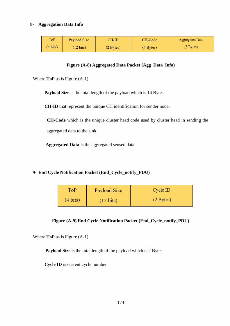
174
8- Aggregation Data Info
Figure (A-8) Aggregated Data Packet (Agg_Data_Info)
Where ToP as is Figure (A-1)
Payload Size is the total length of the payload which is 14 Bytes
CH-ID that represent the unique CH identification for sender node.
CH-Code which is the unique cluster head code used by cluster head in sending the
aggregated data to the sink
Aggregated Data is the aggregated sensed data
9- End Cycle Notification Packet (End_Cycle_notify_PDU)
Figure (A-9) End Cycle Notification Packet (End_Cycle_notify_PDU)
Where ToP as is Figure (A-1)
Payload Size is the total length of the payload which is 2 Bytes
Cycle ID is current cycle number

175
10- Server to Sink Cluster Head re-selection Packet (Reslect_CH_Server_Sink_Packet)
Figure (A-10) Cluster Head re-selection Packet (Reslect_CH_Server_Sink_Packet)
Where ToP as is Figure (A-1)
Payload Size (S) is the variable size that depends number of new cluster heads in the
packet
CL ID contained two field, new CH-ID that represent the unique identification for new
CH, and new CH-Code, which is the unique cluster code used by cluster members and
CH in data transmission.
Time Slot is a node’s transmission time slot
11- Sink to Node Cluster Head re-selection Packet (Reselect_CH_Sink_Node_PDU)
Figure (A-11) Cluster Head re-selection Packet (Reslect_CH_Sink_Node_Packet)

176
Where ToP as is Figure (A-1)
Payload Size (S) is the total length of the payload which is 10 Bytes
CL ID contained two field, new CH-ID that represent the unique identification for the
new CH, and new CH-Code, which is the unique cluster code used by cluster members
and CH in data transmission.
Time Slot is a node’s transmission time slot

177
Appendix B (Protocol Diagram)

178
The Clustering
Calculate the expected range of number of clusters using
Depend on the value of C, centroid nodes will be selected from the nodes
NFV server will Calculate the energy consumption according to the
selected number of clusters
Check all the clusters number
Compare the energy consumption for all number of clusters to find the optimum value that will be used in the network analysis and
thus will minimise the energy consumption in the network
Setup stage
Start steady state stage (data transmission)
Each SNs within the cluster will send it data according to their time slot
and once per cycle
CH for each cluster will aggregate the incoming data from its SNs
and send it to sink according to it time slot
NFV server will build table for each cluster contain (cluster number , SNs IDs within
cluster , their position , their distance to sink )
The NFV server will set a time slot for transmission for each
CH
NFV server will forward the cluster table to the sink which will forward it to the CHs and
nodes
The new round will start again based on Ethreshold (if CHEnergy<Ethreshold)
Eth=Eavg/2
In the new round, the new clsuter head with minimum cost function will be
selected (from the same clsuter)
No
yes
Cluster formation
The cluster head node will be selected based on the minimum cost function.
Depending on the nearest and furthest node to sink dmin<dtoBs<dmax, a range for number
of clusters will be calculated
Start
Discovery Step: Each node with send its packet (node id, message id, node position , energy level ) to the sink, sink will send these information to the NFV server
1- NFV server organize the incoming packets from the sink in the table (SN ID , distance to sink , distance to other SN , SN position , SN cost function)
2- NFV server will calculate the distance between sink and other SN depending on the SNs position and sink position)
NFV server will calculate the cost function for each node using the formula (cost function=dsinksn/Einitial ) and
update the table
NFV will calculate the amount of remaining energy of eaach
node byErem=Einitial-Econsumption
Find distance between these nodes and the other nodes in the network using Euclidian distance
equation, the sensor node will join the best centre node depend on minimum distance
Recalculate the new centre node usingNew CN(x,y)=sum(x of sn)/number of nodes ,
sum(y of sn/number of nodes)
Is CN change
Yes
No
Fix the cluster shape and form the table for the nodes with it
Cluster head selection
1- CN1 will be selected randomly from the sensor
nodes set.2- CN2 will be the
furthest nodes from the CN1.
3- CN3 will be the minimum distance from
the largest set.And so on until reach the
required C
The sink will forward the nodes information to the server
End
The clusters will be reselected when all the nodes within the cluster have been
selected as CH
Appendix C
Virtualised Clustering Routing (VCR) Protocol Flow Chart
Figure (C-1) Virtualised Clustering Routing (VCR) Protocol Flow Chart
Sensor Node’s Energy Monitoring by the server
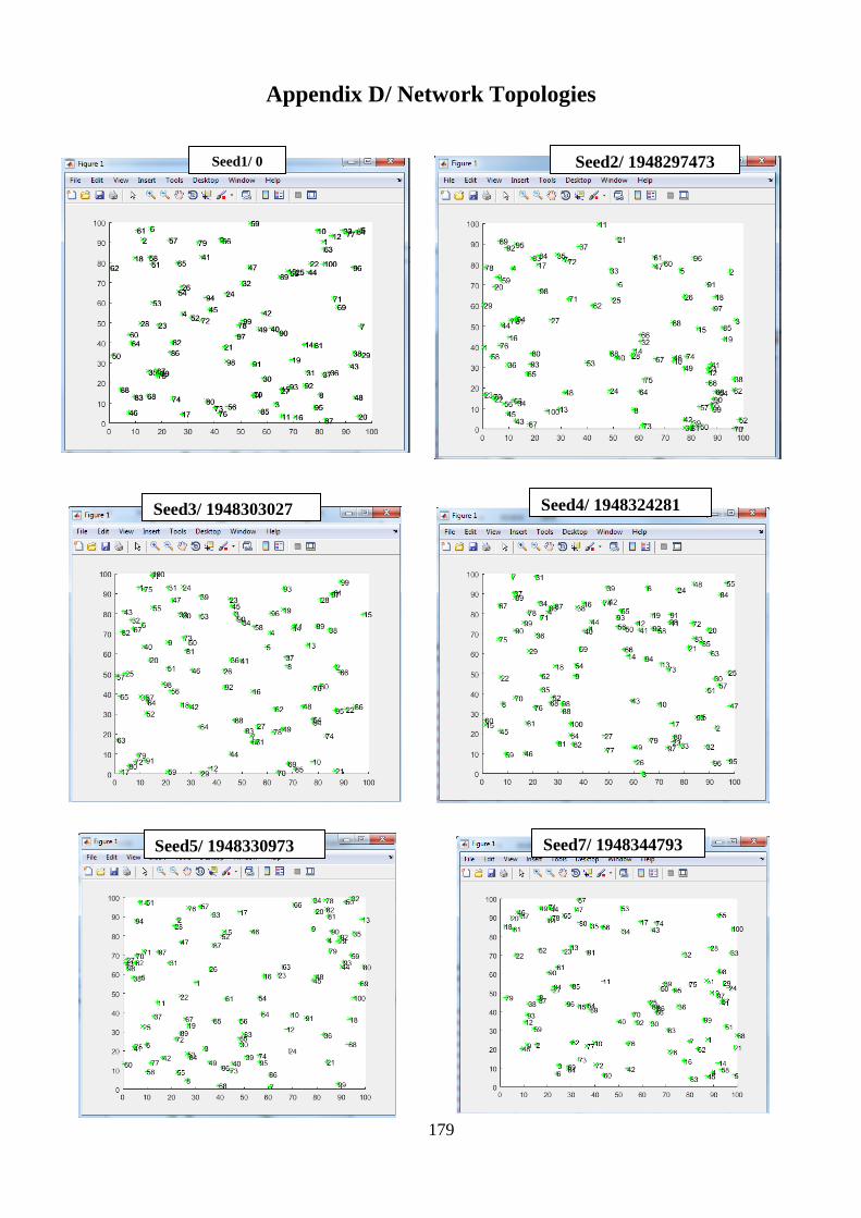
179
Appendix D/ Network Topologies
Seed1/ 0 Seed2/ 1948297473
Seed3/ 1948303027
Seed4/ 1948324281
Seed5/ 1948330973
Seed7/ 1948344793

180
Seed6/ 1948337541
Seed8/ 1948350593
Seed9/ 1948358192
Seed10/ 1948363883
Seed11/ 1948372250
Seed12/ 1948391268

181
Figures (D-1) Network Topologies with various seed values
Seed13/ 1948397202
Seed14/ 1948539028
Seed15/ 1948546874
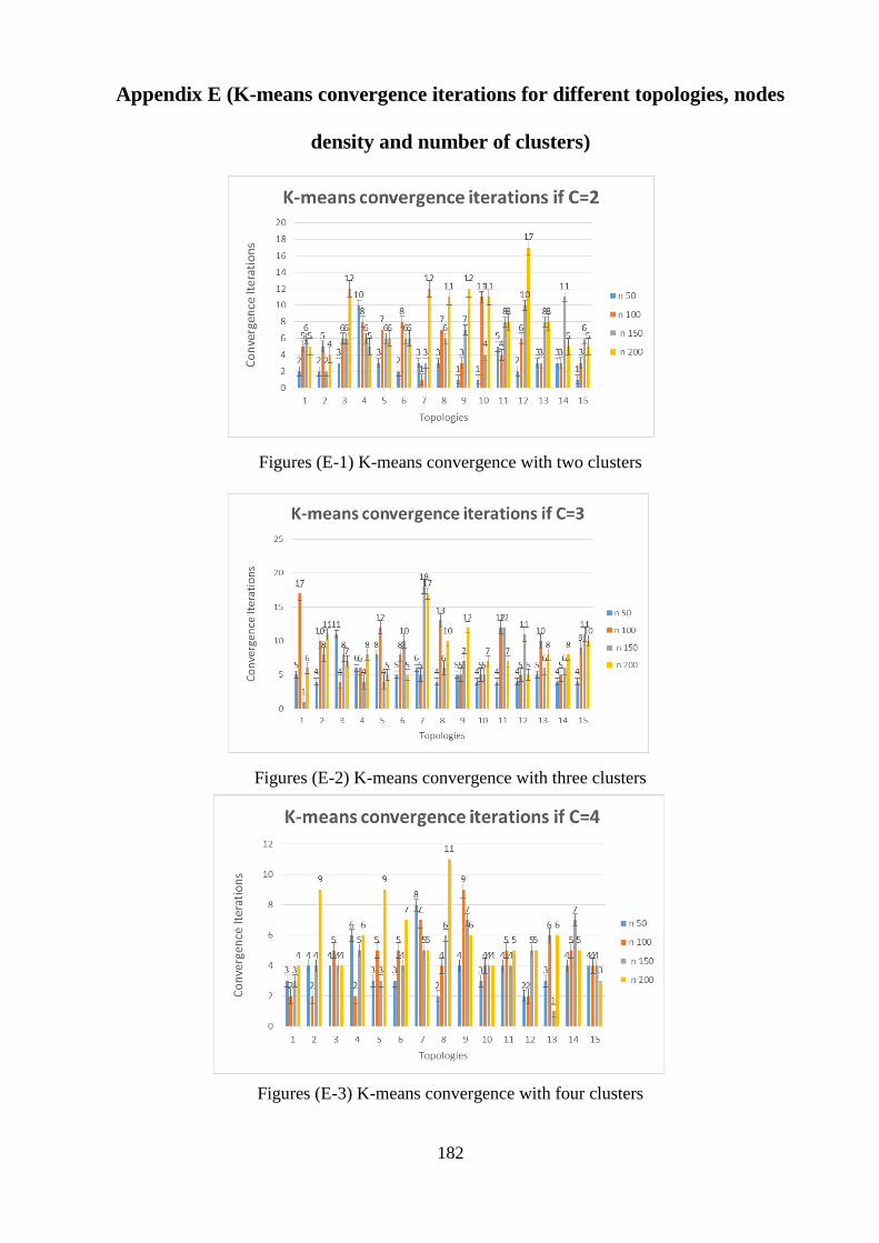
182
Appendix E (K-means convergence iterations for different topologies, nodes
density and number of clusters)
Figures (E-1) K-means convergence with two clusters
Figures (E-2) K-means convergence with three clusters
Figures (E-3) K-means convergence with four clusters

183
Figures (E-4) K-means convergence with five clusters
Figures (E-5) K-means convergence with six clusters
Figures (E-6) K-means convergence with seven clusters

184
Figures (E-7) K-means convergence with eight clusters
Figures (E-8) K-means convergence with nine clusters
Figures (E-9) K-means convergence with ten clusters
Top Related