1

Production Planning under Dynamic Product Environment: A Multi-objective Goal Programming Approach

Boppana V. Chowdary * and Jannes Slomp

Department of Production Systems Design, Faculty of Management & Organization, University of Groningen, P.O. Box 800, 9700 AV, Groningen, The Netherlands. * Corresponding Author

SOM theme A: Primary Processes within firms

Abstract

Production planning is a complicated task that requires cooperation among multiple

functional units in any organization. In order to design an efficient production planning

system, a good understanding of the environment in terms of customers, products and

manufacturing processes is a must. Although such planning exists in the company, it is

often incorrectly structured due to the presence of multiple conflicting objectives. The

primary difficulty in modern decision analysis is the treatment of multiple conflicting

objectives. A formal decision analysis that is capable of handling multiple conflicting

goals through the use of priorities may be a new frontier of management science. The

objective of this study is to develop a multi objective goal programming (MOGP) model to a

2

real-life manufacturing situation to show the trade-off between different some times

conflicting goals concerning customer, product and manufacturing of production planning

environment. For illustration, two independent goal priority structures have been considered.

The insights gained from the experimentation with the two goal priority structures will guide

and assist the decision maker for achieving the organizational goals for optimum utilization

of resources in improving companies� competitiveness. The MOGP results of the study are

of very useful to various functional areas of the selected case organization for routine

planning and scheduling. Some of the specific decision making situations in this context are:

(i). the expected quality costs and production costs under identified product scenarios,

(ii).under and over utilization of crucial machine at different combinations of production

volumes, and (iii). the achievement of sales revenue goal at different production volume

combinations. The ease of use and interpretation make the proposed MOGP model a

powerful communication tool between top and bottom level managers while converting the

strategic level objectives into concrete tactical and operational level plans.

1. Introduction

Production planning is a complicated task that requires cooperation among multiple

functional units in any organization. Planning is the consequence of a hierarchy of decisions

dealing with different issues in the manufacturing environment (Ozdamar et al., 1998). In

order to design an efficient production planning system, a good understanding of the

environment in terms of customers, products and manufacturing processes is a must

(Olhager and Wikner, 2000). A proper production planning within these entities is a key

condition to a manufacturing system success to deal with the limitations of efficiency and

flexibility, and to consider the real world resource limitations (i.e., budget, time, labour,

3

etc.). Although such planning exists in the company, it is often incorrectly structured due to

the presence of multiple conflicting objectives. Therefore, new tools for production planning

are required that consider these issues. To choose between alternative courses of action and

guide managerial decision making, a production manager has to have appropriate

performance criteria (Tabucanon and Majumder, 1989). At the strategic level, these criteria

are usually based on rather broad organizational objectives. For tactical and operations

decisions, however, these general goals have to be converted into more concrete

performance criteria that are amenable to measurement and tracking over time. The primary

difficulty in modern decision analysis is the treatment of multiple conflicting objectives. A

formal decision analysis that is capable of handling multiple conflicting goals through the

use of priorities may be a new frontier of management science. Companies and research are

therefore called upon to develop their own innovative ideas and to expand them to new tools

and procedures. A classical approach to handle this multi-level decision making process is

multi-objective goal programming (MOGP) approach.

Traditionally production plans in any manufacturing organization are developed

through stages, aggregate production plan (APP); master production schedule (MPS); and

short-term production schedule. The APP plays a key role in translating the strategies of the

business plan into an operational plan for the manufacturing process. For example, it allows

managers to determine that whether they can satisfy budgetary goals without having to

schedule the company�s several product models and scarce resources. Even if a planner

could prepare such a detailed plan, the time and effort required to update it would make it

uneconomical. Here the information flows in two directions: from the top down and from

the bottom up. If an aggregate plan cannot be developed to satisfy the objectives of the

business or annual plan, the business or annual plan might have to be adjusted. Similarly, if

a feasible MPS or work force schedule cannot be developed, the aggregate plan might have

4

to be adjusted. Thus, the planning process is dynamic, with periodic plan revisions or

adjustments based on two-way information flows.

The economic significance of APP within firms has been well recognized. But, the

most difficult problem encountered in APP is the fluctuations in product demands. By

allowing overtime or idle time operations of the shop while maintaining a constant

workforce can absorb demand fluctuations. So design of an appropriate production planning

strategy is indeed a dynamic process that relates demand of goods. This decision problem

has been the target of extensive research, and several linear mathematical models for finding

the optimal strategy have since been introduced. In this regard, the reader is referred to Lee

(1972) for a comprehensive review of various mathematical models. However, none of these

suggested methods has found any widespread use in industry. One reason seems to be that

industry is not yet ready to accept the use of formal mathematical models for production

planning. But the primary reason seems to be that the proposed models are gross

oversimplifications of reality, and moreover, they do not provide room to reflect

management�s preferences or policies in the solution.

In reality, however, production planners take a number of objectives into account

during the planning process. The reality can here be expressed as a �customer� demanding

a �product� that is processed through a �manufacturing process�, and we have a production

planning system for the planning and control of the dynamics of these elements as they

interact. All the three entities customer, product, and manufacturing process create a very

complex problem to be solved (Olhager and Wikner, 2000). The qualifiers in the

perspective of production planning system design associated with the three entities are

summarized in Table 1. For instance, under the customer entity, many of the typical

order/market and the order winner qualifiers (e.g. quality, price and different aspects of

flexibility), have large implications for the PPC system. According to Slack et al. (2000),

5

capacity utilization directly affects the speed of response to customers� demand. Hence,

by targeting operations, gains in flexibility, lead time and deliverability will be achieved.

Delivery performance standards (e.g. product volume) relate an operation�s performance

directly to its competitive ability in the market place.

Quite often, most of these goals are competitive in terms of need for scarce

resources. In presence of incompatible goals the manager needs to exercise his judgement

about the importance of the individual goals. Stated more simply, the most important goal

must be achieved to the extent the management desires before the next goal is considered.

In order to achieve the ordinal solution i.e. to achieve the goals according to their

importance, negative and/or positive deviations about the goal must be ranked according

to the �preemptive� priority factors. In this way the low-order goals are considered only

after higher-order goals are achieved as desired (Lee, 1972). Conventional linear

programming is unable to encapsulate this kind of problem directly, as it can only handle

a single goal in the objective function. Of course, by a combination of extensive

modifications of right-hand side values in the constraints and sensitivity analysis, linear

programming could be used, but would be extremely time consuming and unwieldy. The

complexity of the problem can only be addressed explicitly through multi-objective

decision models. Therefore, an effective application of such methods may be possible

only at the expense of changing organizational goals.

In order to solve such multi dimensional planning problems, a flexible and

practical methodology, known as goal programming (GP), was developed by Charnes and

Cooper (1961). Since then many researchers have done a lot of work about extensions of

goal programming methodology (such as preemptive/lexicographic linear goal

programming, integer goal programming (Schniederjans and Hoffman, 1992), extended

lexicographic goal programming (Romero, 2001), etc.) and extensive surveys on fields of

6

its applications (Lee, 1972; Schniederjans, 1995; Tamiz, M., Jones, D., and Romero,1998)

(such as production planning, financial planning, capital budgeting planning, agricultural

running planning, etc.).

Table 1: The three entities for understanding the conditions for production planning environment

Entity Qualifiers in the perspective of production planning system design

Description

Sample performance measure(s) selected for the study presented in this paper

Customer ♦ The order qualifiers -- what is required by the customers

♦ The order winner qualifier � what makes a product offer to a customer a winner

(e.g. quality, price, flexibility)

Analyzing these properties of the customers, we obtain a picture of the customer values and can use this as a point of departure when designing the PPC system

• Product quality

Product Bill of materials (BOM) in order to support aggregate planning and multi-level master scheduling (e.g. product groups, representing the average product in the group, or modules that are assembled to order)

The BOM can be viewed as a hierarchy of deliverables in successive customer-supplier relations

• Production volume

Manufacturing process

♦ Material interface ♦ Transformation process interface

• Depending on the type of planning and control method used, the planning point must be modeled using certain properties, e.g. capacity, capability and process times to sufficiently describe the resources

♦ Resource Interface

The three interfaces are models of reality capturing properties necessary to the PPC system. Also, specifically, the release of discrete orders works as a direct planning mechanism for the manufacturer. The system bottleneck is a key issue for the design of the PPC system. A bottleneck or constraining resource limits the output of the whole manufacturing system, and must therefore be monitored closely with respect to both capacity and material

• Sales Revenue

• Production

costs • Machine

Utilization • WIP

Inventory

7

The objective of this study is to develop a multi objective goal programming model

to a real-life manufacturing situation to show the trade-off between different some times

conflicting goals concerning customer, product and manufacturing of production planning

environment. For illustration, two independent goal priority structures have been considered.

The insights gained from the experimentation with the two goal priority structures will guide

and assist the decision maker for achieving the organizational goals for optimum utilization

of resources in improving companies� competitiveness. The ease of use and interpretation

make the proposed MOGP model a powerful communication tool between top and bottom

level managers while converting the strategic level objectives into concrete tactical and

operational level plans.

1.1. The problem context

The organization selected for the present study is one of the leading precision machine tool

manufacturing firms in India producing standard as well as sophisticated and advanced

machine tools. To maintain the secrecy of data, we hide the company�s name as well as the

exact financial figures while explaining the history of the case organization.

The company is organized in three divisions, namely machine tool, forging &

foundry, and CNC machines. The company at its machine tool division manufactures

various standard machine tools viz., cutter & tool grinder, surface grinder, milling machine

and thread-rolling machine of various models including other CNC versions. The company

has eight market regional offices located all over the country. Sales forecasts were made for

planning production. The sales have exceeded the forecast in a few items and fallen short in

certain other items. A market intelligence cell has been functioning to gather timely

information and developments.

8

For the last several years, the company is running at a loss, though its performance

till then was satisfactory. The loss is due to drop in sales in most of the products and

increase in production overheads. Severe competition was the major reason for drop in sales

in most of the products. The company has a total manpower of 2000, out of which around

60% of the employees� fall under the operator cadre that includes skilled, semi skilled and

unskilled workers.

To promote the clarity of the MOGP approach, the manufacturing case under

study will be limited in scope to the CNC division of the company, which manufactures

CNC lathe and CNC machining centers of various models. According to the management,

the Indian engineering industry is still in the infant stage for introduction of CNC

machines in a large way. These machines are extensively used in automobile industries i.e.

in both local as well as global markets. Whenever there is a boom in this sector, as is the

situation in the country, the demand for the CNC machine tools could be very high. This

puts a pressure on the corresponding production units to step up their production by making

their facilities more efficient and even by increasing their capacities.

In the CNC division there are two NC machines (one each of horizontal miller and

slideway grinder), two CNC machines (vertical miller and horizontal boring) and one

conventional radial drilling machine. Out of the five machines, the major bottleneck had

been the slideway grinding (SWG) operation, which required special skills and was needed

for all parts of the products. The management stated that SWG capacity was not available

with sub-contractors locally, to meet the requirements of the company. Also, the production

manager of the CNC division stated that its capacity was the critical and the deciding factor

while working out the capacity of the whole CNC division. Also, it was observed that there

were more overheads incurred especially with the production of CNC machining centres.

9

However, the quality of products and vigorous drive to capture the market had

given the company an edge over its competitors. The company is holding more inventories

than the norm because of new models fall in demand and to prevent stock-out of imported

items. From the last couple of years, the numbers of CNC lathes sold by company have

declined. The fall in demand was attributed to the adverse economic and market conditions

though products of the company were stated to be popular. The description of the

production environment of the CNC division shows the complexity of their production

planning and multi functions with several product models.

To meet the company�s main objectives, the CNC division has set some objectives

at its divisional level as i) to produce sophisticated, flexible precision machine tools for the

local as well as global markets; ii) flexibility to adapt the product design changes in the

market; iii) to improve productivity and reduce product costs to maintain the market share;

and (iv) to enhance customer satisfaction by offering quality products. For translating these

specific objectives into concrete tactical and operational plans, a GP model under multi-

objective environment has been proposed in this paper to evaluate the trade-offs among the

three entities of the production planning process (refer Table 1).

Section 2 gives brief description of the related literature. In Section 3, multi-

objective model has been developed. Goal programming formulation, its testing with

various goal priority structures and discussion of results is given in Section 4. Finally,

Section 5 summarizes the main conclusions and gives directions for further research.

2. Review of related research

The scope of this literature review is limited to applications of goal programming (GP)

approach to real life manufacturing situations in the multi-objective environment. However,

10

for a rigorous mathematical analysis of multi objective programming approach, the reader is

referred to Steuer (1985). A summary of the selective literature highlighting the specific

problem type with the identified multiple objectives and the solution methodology followed

is presented in Table 2. The multi-objective models in the context of manufacturing were

formulated and solved in the recent past (a few sample studies include Demmel and Askin

1992; Stam and Kuula, 1992; Kim and Schniederjams 1993; Kalpic, Mornar and

Baranovic, 1995; Nagarur, Vrat, and Duongsuwan, 1997) to provide information on

the trade-off among multi-objectives. However, although it represents a viable approach to

production planning, MOGP is not as widespread among manufacturing companies as

desired.

The GP appears to be an appropriate, powerful, and flexible technique for decision

analysis of the troubled modern decision maker who is burdened with achieving multiple

conflicting objectives under complex environmental constraints. The extensive surveys of

the GP by Schniederjans (1995), Tamiz, Jones, and Romero (1998), and Aouni and Kettani

(2001) have reflected this. The modeling approach of GP does not attempt to maximize or

minimize the objective function directly as in the case of conventional linear programming.

Instead of that the GP model seeks to minimize the deviations between the desired goals and

the actual results to be obtained according to the assigned priorities.

11

Table 2: Summary of literature on the application of multi objective modeling approach to various problem environments

Study Type of Problem Environment Multiple Objectives Identified Method Used

Lee and Clayton (1978) Resource allocation in an institution of higher learning

Total cost, salary increase, faculty/student ratio, faculty/graduate assistant ratio

Goal Programming

Sundaram (1978) Selecting levels of machine parameters in a fine turning operation

Finish turning depth in one pass, finish turning with in a stipulated time.

Goal Programming

Singh and Agarwal (1983) Determination of the optimum size of extended octagonal ring

Sensitivity, rigidity Goal Programming

Stam and Kuula (1991) Selection of a flexible manufacturing system Production volume, cost, flexibility Goal Programming Shafer and Rogers (1991) Formation of manufacturing cells Min. setup time, Min. intercellular

movements, Min. the investment in new equipment, Maintain acceptable utilization levels

Goal Programming

Premchandra (1993) Activity crashing in project networks Crashing time of an activity, Project cost, Project time

Goal Programming

Kim and Schniederjams (1993)

Just-in-time manufacturing Production smoothing, balancing of production line, number of kanbans, setup time, idle and overtime, production cost

Multi Objective Programming

Lyu, Gunasekaran, Chen and Kao (1995)

Coal blending Demand of each boiler, environmental requirement of the sulphur oxide emission, heating value requirements, volatile matter content requirement, ash content requirement, inventory.

Goal Programming

Nagarur, Vrat, Duongsuwan (1997)

Production planning and scheduling for injection moulding of pipe fittings

Goal Programming

Shang and Tadikamalla (1998)

Design and control of a cellular manufacturing system

Flow time, waiting time, work-in-process inventory

Simulation with optimization techniques such as Taguchi method and response surface methodology

Su and Hsu (1998) Machine-part cell formation Total cost, intracell machine loading unbalance, intercell machine loading unbalance

Simulated annealing

Zhao and Wu (2000) Manufacturing cell formation problem Minimizing costs due to intercell and intracell part movements, Minimizing the total within cell load variation, Minimizing the exceptional elements

Genetic algorithm approach

Linares and Romero (2000)

Electricity planning Min. total cost, CO2, SO2, NOx emissions, amount of radio active waste produced

AHP

Wang, Shaw, Chen (2000) Machine selection in flexible manufacturing cell (FMC)

Purchasing cost, machine floor space, machine number, productivity of the FMC

Fuzzy MADM approach

12

Therefore, the GP model handles multiple goals in multiple dimensions (Sundaram, 1978).

Further, the distinguishing characteristic of GP is that it allows for an ordinal solution (Lee,

1972). Stated differently, management may be unable to specify the cost or utility of a goal,

but often upper or lower limits may be stated for each goal. A commonly used generalized

model for goal programming is as follows (Kwak et al. 1991):

minimize Z = Σi wi Pi (di+ + di

-)

subject to

Σjaijxij + di- - di

+ = bi (i = 1,2,�,m),

xij , di- , di

+ ≥ 0

(i = 1, 2,�, m; j = 1, 2, �, n)

where Pi is the preemptive factor/priority level assigned to each relevant goal in rank order

(i.e. P1 > P2 > � Pn), and wi are non-negative constants representing the relative weights

assigned within a priority level to the deviational variables, di+ and di

- , for each j-th

corresponding goal, bi. The xij represents the decision variables, aij represents the decision

variable coefficients.

From the literature it is clear that the GP approach has been applied for a variety

of applications. Examples of problems solved by GP technique are resource allocation in

an institution of higher learning (Lee and Clayton 1978), selecting levels of machining

parameters (Sundaram 1978), determining optimum size of a machined component (Singh

and Agarwal 1983), production planning in a ship repair company (Tabucanon and

Majumdar 1989), cell formation problem (Shafer and Rogers 1991), activity crashing in

project networks (Premchandra 1993) and production smoothing under just-in-time

manufacturing environment (Kim and Schnierderjams 1993). The applicability of MOGP

to the planning decisions have been established (Kwak et al. 1991, Giokas and

Vassiloglou, 1991). Linear MOGP approach has successfully been applied for the

13

planning objectives include calculating the optimum production mix and achieving the

capacity and material balance, while maximizing the contribution and minimizing the

duration of the longest resource management (Kalpic, Mornar, and Baranovic, 1995).

Another application illustrated the use of zero-one GP for the development of a production

planning and scheduling model in a injection moulding factory with an objective to

minimize the total costs of production, inventory, and shortages (Nagarur, Vrat and

Duongsuwan, 1997).

It appears that production planning is an area where GP can be applied very

efficiently. The primary reason is, of course, that there are only limited human factors

involved in decision analysis. Therefore, the future outcome can be forecast with a

greater accuracy. Also, it is apparent from the literature that, the GP technique has

potential to solve the conflicting aspects of the three entities, namely, customer, product

and manufacturing process of the manufacturing firm under consideration. As far as the

authors know, MOGP is not used for this purpose so far. Furthermore, quantification of

the performance criteria of these three entities is a challenging task. In this regard, we

propose a linear multi objective goal programming model to a machine tool

manufacturing industry to illustrate the impact of variations in product demand on the

firm performance by evaluating the trade-off among the three entities.

3. The multi-objective model

Good products with improved quality and styles can promote customer demand to a

certain degree, thereby increasing revenues. A revenue increase, however, is not always

possible because customers usually determine the selling price and the demand is highly

uncertain and fluctuating. Unless a company manufactures superior products just in time,

14

the products may not be sold, piling up inventories. Even the products already sold could

be recalled or returned, eventually making the company out of business (Son, 1994,

pp.443). Short lead times and a high schedule performance determine the companies

logistical quality, where as high and steady utilization of the production facilities and low

WIP inventory influence the profitability of the production process. Problems occur due to

the fact that these objectives are partly conflicting.

As world class companies have proved that the product quality is one of the major

strategic factors in managing manufacturing systems. Studies of Son (1993) state that

increased product quality can be measured by reduced quality cost and increased customer

satisfaction can be measured by reduced external failure costs (p.419). Improving product

quality is now at the top of a manufacturer�s priority list. Quality control professionals

(Juran 1951 and Feigenbaum, 1961) first developed the concepts of �quality cost� and have

been recognized by the practitioners widely. For better quality management, quality should

be convertible to monetary terms since dollars are the easiest and most effective

communication language (Son and Hsu , 1991). Quality cost is usually broken down into

four categories of appraisal, prevention, internal failure and external failure costs and most

of them are costable. While building MOGP model, we reduce these four categories to two:

prevention (that includes appraisal cost) and failure (that include external and internal costs)

in the similar lines as that of Son and Hsu (1991). Here prevention cost is redefined as the

cost of preventing product defects by checking and correcting in-process quality problems

before final inspection. And failure cost is redefined as the loss due to failure of finished

products to meet quality standards set by both a company and its customers.

As a result of market dynamics and fierce global competition, it is felt that crucial

performance criteria regarding to customer satisfaction should be considered in the

planning process. Also, the manufacturing firm under consideration is forced to provide a

15

better quality product on a more cost-effective basis while significantly reducing

processing waste such as rework and scrap. To focus on these issues, and after discussing

with the quality control department professional of the case study, we separated the

quality cost component from the production cost and categorized under customer�s goal.

In practice, however, it will not be the case with many of the practitioners. Also, due to

the capital-intensive nature of the products (machine tools) of the firm under

consideration, it is assumed that the planning horizon as one year. Because, the top

management sets the company�s strategic objectives for at least the next year in the

business plan, which facilitates the overall framework of demand projections, functional

area inputs, and capital budget from which the aggregate plan can be developed.

In a machine constrained production system, a key issue is how to evaluate the

crucial resource use for varying demand opportunities. There is, therefore, a certain

machine over or idle capacity will exists. If there is any idle capacity, it can be used for to

meet the excess product demands. But on the other hand if there is any over capacity, then

the management must be plan to meet this situation through someway or other. For

instance, operate the crucial resources either on overtime basis or create an additional

capacity by adding new machines to the existing system. Important then is how to

evaluate the crucial resource use in the dynamic product mix and volume scenarios. As

mentioned in the introduction, this situation occurs frequently in the selected case study

especially with the operation of SWG. In this bottleneck scenario, the capacity evaluation

of SWG is suggested as one of the multi-objectives of the study.

Performance measures are selected to achieve goals and are provided with the

intent to monitor, guide and to communicate to all the business functions in an effective

way between the top and the bottom level managers of the manufacturing firm under

consideration. In the past, many researchers have attempted the manufacturing

16

performance evaluation problem in terms of various performance measures. In

consultation with the shop floor and marketing mangers of the selected machine tool

industry, various performance measures (that representing the conditions of customer,

product, manufacturing process) such as sales revenue, quality costs, capacity utilization,

production cost, WIP inventory and production volume were identified as crucial

measures of the study for building a linear MOGP model (refer, Table 1). But the selected

performance criteria of the three entities of the production planning system are interrelated

and often conflicting in nature. For instance, more precision and flexible products of the

manufacturer obviously provide more satisfaction to the customer, but it can take time to

incorporate any major design changes in the existing product design especially in the

present case situation. The true value of MOGP approach is, therefore, the solution of

problems involving multiple conflicting objectives according to the management�s

preferences towards their attainment. The details of variables, and the objective functions

representing the various performance criteria are presented as follows.

Notation

Indices

i = Product type (i = 1, 2,.., n)

j = Machine (non-crucial) type (j = 1,2,..,m)

Parameters

ai = SWG machine capacity required for processing of product i

ci = Production cost of i th product

oij = Capacity required for the i product from j th non-crucial machine

qi = Quality costs incurred on i th product

17

si = Sales revenue from i th product

wi = Cost of work-in-process inventory associated with i th product

CAPj = Total available capacity of the j th non-crucial resource.

Decision variable

xi = Production volume(number of machines) of type i to be produce per period

3.1 Development of the multi objectives

The problem considered here involves the production planning of two different product

types, CNC machining centre and CNC lathe using the existing manufacturing facilities

include one SWG, which is of crucial type and four non-crucial machines. As mentioned

earlier, the firm is experiencing severe competition from the local as well as global

markets. There is an urgent need to increase the product quality as well as customer

satisfaction. Also, the management wants to avoid under utilization of SWG. At the same

time it wants to operate SWG on overtime to maintain good employer-employee relations,

minimize production overheads, quality costs, WIP inventory costs and to maximize the

gross sales margin of the plant as much as possible. In this regard, the top management is

to make a decision that will achieve these objectives of the three entities as closely as

possible with the minimum sacrifice. The following performance criteria are incorporated

in the model: (i) quality cost; (ii) production volume of each product (iii) production cost;

(iv) SWG utilization, (v) cost of work-in-process inventory; and (vi) sales revenue. These

important criteria are formulated as:

Minimize quality costs, QC = Σi qi xi ... (1)

Maximize production volume, V = xi ,for all i ... (2)

18

Minimize production costs, C = Σi ci xi ... (3)

SWG utilization, U = Σi ai xi ...(4)

Minimize work-in-process inventory cost, W = Σi wi xi ...(5)

Maximize sales revenue, SR = Σi si xi ...(6)

Σi oij xi ≤ CAPj ,for all j ...(7)

Equations (1) to (6) represent functional relationship between the production volumes of

product i (decision variable), and the various performance measures of the three entities.

Where as equation (7) denotes the system constraints.

The equation (1) ensures the condition of the customer satisfaction in terms of final

product quality. The parameter qi can be represented in terms of different product quality

costs. The total production volume per period of all products is represented through the

objective (2). This equation closely resembles to that production volume criteria given by

Stam and Kuula (1991). Equations (3-6) represent the conditions of the manufacturing

process. The total cost of production per product is represented as ci * xi in equation (3). Here

ci is nothing but the unit cost of production excluding product quality costs, which is the

sum of machine costs, tool costs, parts pallets costs, software costs, transportation costs and

other costs and this is represented through the parameter. The SWG machine capacity

utilization can be obtained through the equation (4), which will directly affects the speed of

response to customers� demand (Slack et al. 2000). Work-in-process inventory is one of the

crucial performance measures of the case study. This can be computed through equation (5).

Finally, the objective of sales revenue is formulated through equation (6), which is

represented as si * xi for the i th product. It is clear that many of the above performance

criteria are conflicting, and that the decision problem of evaluating their trade-off is a

19

complicated one. In such a conflicting multi objective environment the conditions of the

three entities should be appropriately treated to reflect the decision makers� targets on

various performance criteria into the planning process through an ordinal hierarchy. Due to

these reasons only a goal programming solution approach for the above model has been

sought. The details of the formulation of the problem in goal programming format are

presented below.

4 Formulation of the problem in goal programming format

4.1 Estimation of parameters of the GP model

To formulate the model, the parameters used for input to the GP model in each priority

structure should be given or else estimated by the company. Therefore, the company

personnel are get involved and also encouraged to take a major role in formulation. All

model parameters are assumed to be deterministic and constant during planning horizon. As

mentioned earlier, the planning horizon is taken as one year. The management is mainly

focused on the SWG operation while formulation of the capacity utilization goal. Because it

is only the bottleneck machine within the CNC division of the company. The parameters

and estimation of their values are described below.

4.1.1. SWG capacity required (ai ) /and available (A)

This is estimated based on the time needed for machining of one unit of product i

on slideway grinder (SWG). Average setup times of the products are also taken into

consideration in the fixation of ai. The average manufacturing time for each product i on

SWG is obtained from the process plan. The production manager of the company provides

20

the capacity available in the planning horizon for each non-crucial machines (m = 4, in the

present case study). Factors such as allowances for planned maintenance and average

breakdown times are calculated from past data. Special holidays are also taken into

consideration in the computation of net available times of the machines. In the existing

operational environment, the shop floor managers calculate the available capacity of the

SWG as well as other non-crucial machines as 4500 hours per year.

4.1.2. Production cost (ci)

The total cost of production per product is estimated as the sum of machine costs,

tool costs, parts pallet costs, software costs, internal transportation costs and other costs.

Only direct investment costs are included in the machine costs. The tool costs are estimated

based on the complexity of the products and the number of tools needed. The management

in consultation with the operations management department decides the production cost

parameter.

4.1.3. Quality cost (qi)

If the customer quality is increased, the costs of providing the effort � through extra

quality controllers, inspection procedures, and so on � increases proportionally (Slack et al.

2000; p.823). These costs of quality are taken as the sum of prevention and failure costs.

The company quality norms are followed while estimation of this parameter.

4.1.4. Sales revenue (si)

This parameter depends on the company�s sales target in the planning horizon. The

demand is forecasted by the marketing department of the company, and is assumed to be

deterministic. The marketing department estimates unit sales contribution from each product

by using the previous year�s sales data.

21

4.1.5. Work-in-process inventory (wi)

This is taken as the opportunity cost of the capital blocked in inventory as work-in-

process. Due to frequent introduction of new product models and to prevent stock-out of

imported items, this value is taken as 30% annual rate on the production cost. This cost is

assumed to be constant over the planning horizon.

4.2 Model formulation

1. Customer�s goal: product quality

Final product quality is expected to be 100 percent to satisfy the customer fully. As

mentioned earlier, this can be represented in terms of different quality cost components. At

the same time the sum of these components should be maintained at minimum level.

Satisfaction of the customer goal of product quality can be represented as

minimize (d1+ )

subject to

Σiqixi + d1- - d1

+ = 0 ... (8)

where

xi = product volume of i to be produced to fulfill the customer�s quality requirements,

i = 1, 2 (selected CNC division is producing only two product types)

d1+, d1

- = over and under achievements of quality goal.

Here, the underachievement of the quality goal is allowed and hence negative deviation is

not included in the objective function. The solution will consists all x�s which satisfy Σiqixi

≤ 0, provided such a solution set is possible. If the model cannot minimize d1+ to zero, the

solution consists of all x�s which minimize Σiqixi to the possible extent.

22

2. Market goal: meet aggregate product volumes

Market requirements with respect to aggregate product volumes of product 1 and product 2

(i.e. sum of all customer orders in the planning period) are to be met. Here, exact

achievement of the product volumes is desired and hence both negative and positive goal

deviations must be considered in the objective function. This goal can be represented as

minimize (d+2 + d-

2 + d+3 + d-

3)

subject to x1 + d2- - d2

+ = V1 ... (9), and

x2 + d3- - d3

+ = V2 ... (10)

where

d2+ = over achievement of product 1 volume goal

d2- = under achievement of product 1 volume goal

d3+ = over achievement of product 2 volume goal

d3- = under achievement of product 2 volume goal

V1 = market goal on product 1 volume (aggregate) as per prediction (goal)

V2 = market goal on product 2 volume (aggregate) as per prediction (goal)

Here, minimization of d (.)- + d (.)

+ will minimize the absolute value of x(.) � V(.). In other

words, minimization of both negative and positive deviations of product volume will tend

to search for the x1 and x2 which achieves the goal x (.) = V (.) exactly.

3. Sales revenue: manufacturer�s goal

In view of past sales records and increased customers� awareness towards factory

automation, the management feels that the sales goal for the next year should be �S� million

rupees. And, achievement of the sales revenue goal, which will be set at S, is a function of

23

total gross margin of the product1 and product 2 respectively. This goal can be represented

as

minimize (d4- )

subject to

Σisi xi + d4- - d4

+ = S ... (11)

where

d4- = under achievement of the sales revenue goal

d4+ = over achievement of the sales revenue goal

S = sales revenue goal fixed by the management.

Here, the over achievement of sales goal is acceptable, and hence positive deviation from

the goal is eliminated from the objective function. The solution set will consist of all x�s

such that Σisi xi ≥ S by minimizing d4- to zero, if such solutions are possible in the

model. If it is not possible to minimize d4- to zero, the solution set will consist of all x�s

that minimize (S -Σisi xi) to the extent possible.

4. Production cost: manufacturer�s goal

The manufacturer�s goal of minimizing the production cost for the product volumes of

product 1 and product 2 can be represented as

minimize (d5+ )

subject to

Σicixi + d5- - d5

+ = 0 ... (12)

where

d5- = under achievement in production cost goal

d5+ = over achievement in production cost goal

24

Here, the solution will identify all x�s which satisfy Σicixi ≤ 0, provided such a solution is

possible. If the model cannot minimize (d5+) to zero, the solution consists of all x�s which

minimize Σicixi to the fullest possible extent.

5. Utilization of SWG: manufacturer�s goal

The management of the case study believes that a good employer-employee relationship is

an essential factor of business success. Therefore, they feel that a stable employment level

with occasional overtime requirement is a better practice than an unstable employment with

no overtime. Hence the positive deviation from the goal can be eliminated from the

objective function. The manufacturer�s goal of minimize the under utilization of SWG

machine can be represented as

minimize (d6-)

subject to

Σiaixi + d6- - d6

+ = A ... (13)

where

A = available capacity of the SWG machine (goal)

d6+ = over time required for operation of SWG machine

d6- = idle capacity of SWG machine

Here, the solution will identify all x�s such that Σiaixi ≥ A, by minimizing negative deviation

to zero, if such a solution is possible in the model.

25

6. Work-in-process inventory: manufacturer�s goal

At present the company is holding more work-in-process (WIP) inventory than the norms.

Due to this, the manufacturer�s goal of minimizing WIP inventory for the production

volumes of product1 and product2 can be represented as

minimize (d7+ )

subject to

Σiwixi + d7- - d7

+ = 0 ... (14)

where

d7+ = over achievement in WIP inventory goal

d7- = under achievement in WIP inventory goal

Here, the under achievement of the WIP inventory goal is encouraged and hence negative

deviation is not included in the objective function. Also, the solution set will consist all x�s

which satisfy Σiwixi ≤ 0, provided such a solution space is possible. If the model cannot

minimize (d+) to zero, the solution consists of all x�s which minimize Σiwixi to the possible

level.

4.3 Sensitivity to changes in the goal priority structures

In order to test the GP model, two independent goal priority structures have been formulated

based on the preferences that the company�s top management expressed especially to suit

specific market conditions. A goal priority structure is nothing but a hierarchical

representation of the goal priorities, which reflect the decision makers� preferences.

Production and marketing personnel were actively involved in the selection and prioritizing

of the various goals. In addition to variables and constraints (from 9-15) stated above the

26

following �preemptive� priority factors for the two finalized goal priority structures (for

summary, refer Table 3) are defined.

Goal Priority Structure #1

P1 = the highest priority is assigned by the management to the satisfaction of product

demand. Both the negative and positive deviations (i.e. d+2 + d-

2 + d+3 + d-

3)

from product1 and product2 demands should be minimized.

P2 = the second highest priority factor is assigned to the minimization of over

achievement of quality cost goal (i.e. d+1) to meet customer�s quality

requirements.

P3 = the last priority factor is assigned to the manufacturing process goals i.e.

minimization of under achievement of sales revenue (d-4); minimization of over

achievement of production cost (d+5); minimization of underutilization of SWG

machine (d-6); and minimization of over achievement of WIP inventory (d+

7).

Now the model for this priority structure #1 can be formulated. The objective is the

minimization of deviations from various goals imposed by the production planning

environment. The deviant variable(s) associated with the highest preemptive priority (P1)

must be minimized to the fullest possible extent. When no further improvement is possible

in the highest goal, then the deviations associated with the next highest priority factors (in

the order of P2, P3) will be minimized. The model can be expressed as:

minimize Z1: P1 (w2-d2

- + w2+d2

+ + w3-d3

- + w3+d3

+ ) + P2 (w1+d1

+) + P3 (w4-d4

- +

w5+d5

+ + w6-d6

- + w7

+d7+

) � (15)

subject to goal constraint (9) - (14) and

27

x1, x2, d1-, d1

+, d2-, d2

+, d3-, d3

+, d4-, d4

+, d5-, d5

+, d6-, d6

+, d7-, and d7

+ ≥ 0.

Where w(.) (.) are non-negative constants representing the relative weights assigned within a

priority level to the deviational variables.

Goal Priority Structure #2

Under the priority structure #1, the product demand goal for product1 and product2

was fixed as the top most priority by the management. But as per the problem

context the company has experienced decline in demand for the product2 and also it

is holding more inventories than the norm. To reflect these issues especially to see

the trade-off among various performance measures, within the priority structure #2,

suppose the production volume goal of product2 is now of utmost important and is,

therefore, given top priority. That is, to stay in the business, selling of product2 has

become company�s first and foremost important priority. However, it is worth to

note that this is only possible through customer�s satisfaction i.e. through enhancing

the quality of the product. The MOGP approach provides the decision makers with

the flexibility they desire and is able to offer them an optimal solution. This is an

important advantage of goal programming, allowing the decision makers to evaluate

28

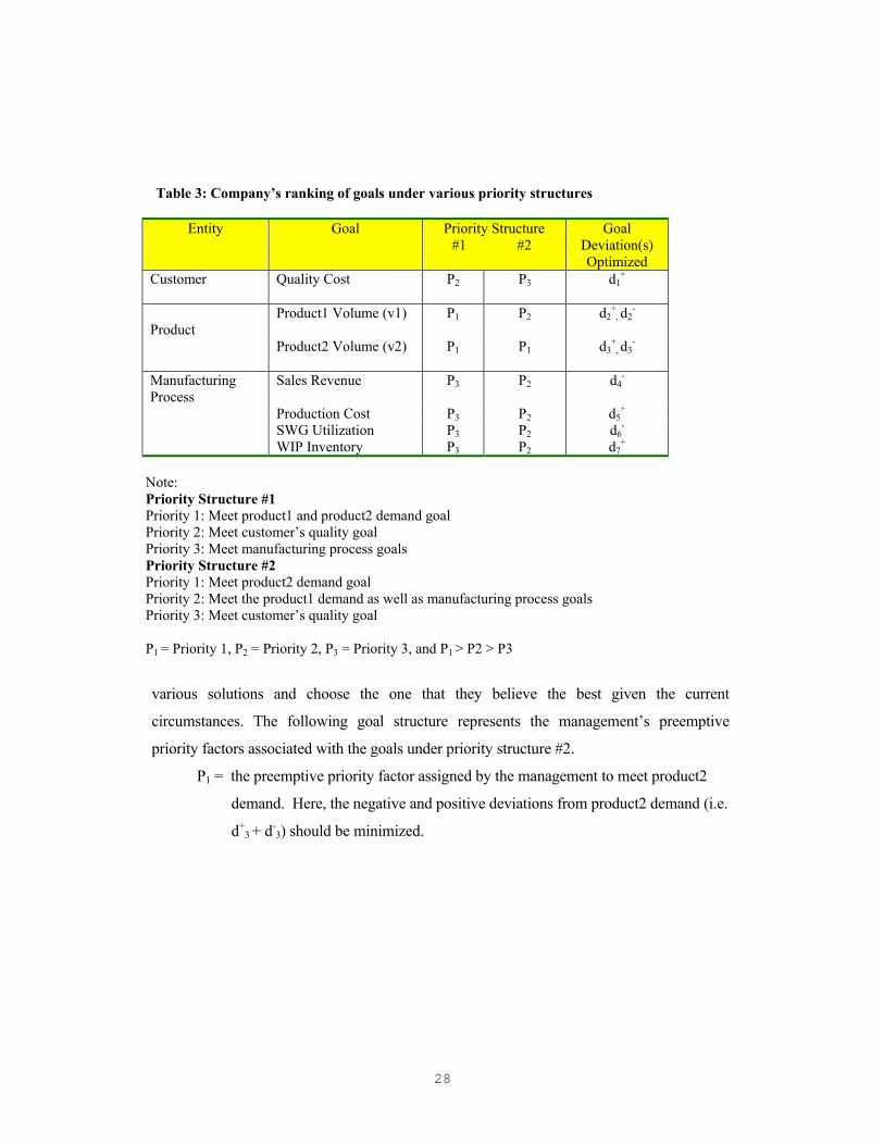
Table 3: Company�s ranking of goals under various priority structures

Entity Goal Priority Structure #1 #2

Goal Deviation(s) Optimized

Customer Quality Cost P2 P3

d1+

Product

Product1 Volume (v1) P1 P2

d2+

, d2-

Product2 Volume (v2)

P1 P1 d3+

, d3-

Manufacturing Process

Sales Revenue P3 P2 d4-

Production Cost P3 P2 d5+

SWG Utilization P3 P2 d6-

WIP Inventory P3 P2 d7+

Note: Priority Structure #1 Priority 1: Meet product1 and product2 demand goal Priority 2: Meet customer�s quality goal Priority 3: Meet manufacturing process goals Priority Structure #2 Priority 1: Meet product2 demand goal Priority 2: Meet the product1 demand as well as manufacturing process goals Priority 3: Meet customer�s quality goal P1 = Priority 1, P2 = Priority 2, P3 = Priority 3, and P1 > P2 > P3

various solutions and choose the one that they believe the best given the current

circumstances. The following goal structure represents the management�s preemptive

priority factors associated with the goals under priority structure #2.

P1 = the preemptive priority factor assigned by the management to meet product2

demand. Here, the negative and positive deviations from product2 demand (i.e.

d+3 + d-

3) should be minimized.

29

P2 = the second priority factor is assigned to the manufacturing process and product1

demand goals i.e. minimization of under achievement of sales revenue (d-4);

minimization of over achievement of production cost (d+5); minimization of

underutilization of SWG (d-6); minimization of excess WIP inventory (d+

7); and

minimization of the negative and positive deviations from product1 demand

(i.e. d+2 + d-

2).

P3 = the lowest priority factor is assigned to the minimization of over achievement

(i.e. d+1) of quality cost goal.

Now the overall model for the priority structure #2 can be represented as:

minimize Z2: P1 (w3-d3

- + w3+d3

+) + P2 (w2-d2

- + w2+d2

+ + w4-d4

- + w5+d5

+ + w6-d6

- +

w7+d7

+ ) + P3(w1+d1

+) � (16)

subject to goal constraint (9) - (14) and

x1, x2, d1-, d1

+, d2-, d2

+, d3-, d3

+, d4-, d4

+, d5-, d5

+, d6-, d6

+, d7-, and d7

+ ≥ 0.

In the above model, Z2 in the objective function can be interpreted as the total of the

unattained portions of production planning goals. And w(.) (.) are non-negative constants

representing the relative weights assigned within a priority level to the deviational variables.

4.4 Model results and discussion

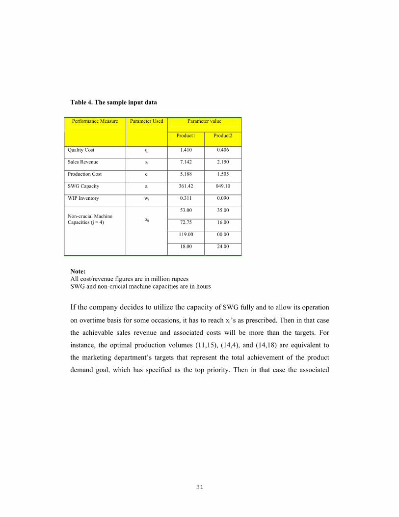
The proposed MOGP model is tested using as the inputs, the firm�s data for a

specific one year period. A sample of the input data is given Table 4, for both of the

preemptive goal priority structures. Each priority structure was executed using

LINGO software package (LINDO Systems Inc. 1999) with P1 = 100, P2 = 10, and P3

=1, which are finalized based on the policies of the management of the case study.

30

Also, the non-negative constants representing the relative weights assigned within a

priority level to the deviational variables are set at a value of one. The sensitivity

analysis for the two goal priority structures was carried out for different

combinations of tentative product demands specified by the company�s marketing

division. The solution obtained under the priority structure #1 is considered

appropriate by the management under the current situation. But marketing

conditions may change from time to time that require a restructuring of the goals to

suit the circumstances. To illustrate the power of GP, a different solution

representing a different prioritization of the same goals was investigated. The

solution (under priority structure #2) that was generated will be discussed

immediately, following a discussion of priority structure #1 solution. The output for

the two different goal priority structures is shown in Table 5-6. The trade-offs

among the various performance measures and the optimized production volumes

were tabulated (Table 7-8). Inferences drawn from the results are presented below:

Priority structure #1

To operationalize the MOGP solution obtained under the priority structure#1, marketing

department should supply their products, namely, CNC machining centre and CNC lathe

to the prescribed customers according to the optimal production volumes defined by the

model�s resulting xi�s. The optimal and maximum possible measures such as sales

revenue, quality cost, production cost and WIP inventory cost are summarized in Table 7.

31

Table 4. The sample input data

Parameter value Performance Measure Parameter Used

Product1 Product2

Quality Cost qi 1.410 0.406

Sales Revenue si 7.142 2.150

Production Cost ci 5.188 1.505

SWG Capacity ai 361.42 049.10

WIP Inventory wi 0.311 0.090

53.00 35.00

72.75 16.00

119.00 00.00

Non-crucial Machine Capacities (j = 4)

oij

18.00 24.00

Note: All cost/revenue figures are in million rupees SWG and non-crucial machine capacities are in hours

If the company decides to utilize the capacity of SWG fully and to allow its operation

on overtime basis for some occasions, it has to reach xi�s as prescribed. Then in that case

the achievable sales revenue and associated costs will be more than the targets. For

instance, the optimal production volumes (11,15), (14,4), and (14,18) are equivalent to

the marketing department�s targets that represent the total achievement of the product

demand goal, which has specified as the top priority. Then in that case the associated

32

revenue and cost figures are nothing but the optimal values. Whereas in the other product

scenarios (7,7), (2,8), and (8,4) (refer Table 7), the optimal x1 and x2 are higher than the

targets (due to positive deviation in product1 volume, refer Table 5). The suggested

production volumes are justifiable due to the idle capacity of SWG at the target volumes

and also the company is trying to regain its market share through its product quality

campaigns. At the suggested production volumes of the model, the associated costs and

sales revenue will be on higher side. For example, the optimal sales revenue figures at the

targeted product scenarios (7,7), (2,8), and (8,4) are 65.04, 31.48, and 65.74 million

rupees i.e. if the company is able to supply only the targeted product volumes. But if the

marketing department is able to sell all the produced machines i.e. (11,7), (11,8), and

(11,4) then the company�s tentative sales revenue at these volumes will be 96.59, 98.73,

and 90.13 million rupees respectively.

33

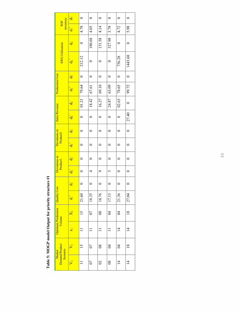
Tab

le 5

: MO

GP

mod

el O

utpu

t for

pri

ority

stru

ctur

e #1

Mar

ket

Dem

and/

Prod

uct

Scen

ario

Opt

imum

Pro

duct

ion

Vol

ume

Q

ualit

y C

ost

Dev

iatio

ns in

Pr

oduc

t1

Dev

iatio

ns in

Pr

oduc

t2

Sale

s Rev

enue

Pr

oduc

tion

Cos

t SW

G U

tiliz

atio

n W

IP

inve

ntor

y

V1

V2

x 1

X2

d 1+

d 1-

d 2+

d 2-

d 3+

d 3-

d 4+

d 4-

d 5+

d 5-

d 6+

d 6-

d 7+

d 7-

11

15

11

15

21.6

0 0

0 0

0 0

0 01

.21

79.6

4 0

212.

12

0 4.

78

0

07

07

11

07

18.3

5 0

4 0

0 0

0 18

.42

67.6

1 0

0 18

0.68

4.

05

0

02

08

11

08

18.7

6 0

9 0

0 0

0 16

.27

69.1

0 0

0 13

1.58

4.

14

0

08

04

11

04

17.1

3 0

3 0

0 0

0 24

.87

63.0

9 0

0 32

7.98

3.

78

0

14

04

14

04

21.3

6 0

0 0

0 0

0 02

.63

78.6

5 0

756.

28

0 4.

72

0

14

18

14

18

27.0

4 0

0 0

0 0

27.4

0 0

99.7

2 0

1443

.68

0 5.

98

0

34

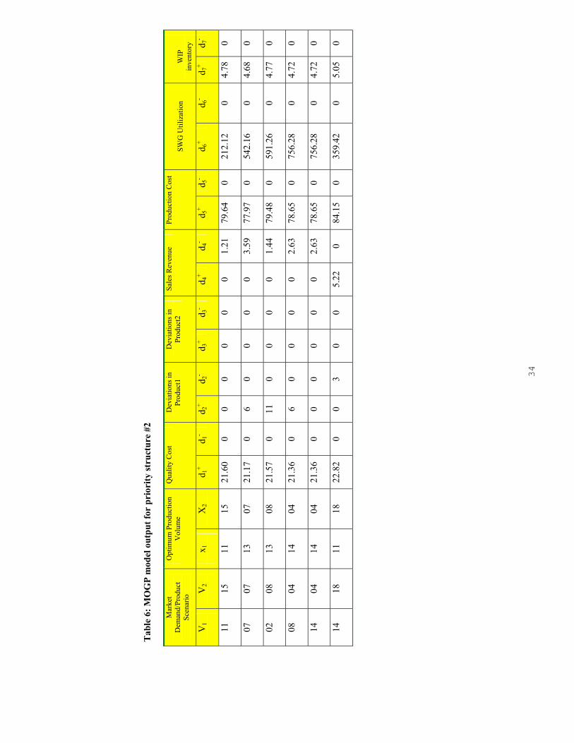
Tab

le 6

: MO

GP

mod

el o

utpu

t for

pri

ority

stru

ctur

e #2

Mar

ket

Dem

and/

Prod

uct

Scen

ario

Opt

imum

Pro

duct

ion

Vol

ume

Q

ualit

y C

ost

Dev

iatio

ns in

Pr

oduc

t1

Dev

iatio

ns in

Pr

oduc

t2

Sale

s Rev

enue

Pr

oduc

tion

Cos

t SW

G U

tiliz

atio

n W

IP

inve

ntor

y

V1

V2

x 1

X2

d 1+

d 1-

d 2+

d 2-

d 3+

d 3-

d 4+

d 4-

d 5+

d 5-

d 6+

d 6-

d 7+

d 7-

11

15

11

15

21.6

0 0

0 0

0 0

0 1.

21

79.6

4 0

212.

12

0 4.

78

0

07

07

13

07

21.1

7 0

6 0

0 0

0 3.

59

77.9

7 0

542.

16

0 4.

68

0

02

08

13

08

21.5

7 0

11

0 0

0 0

1.44

79

.48

0 59

1.26

0

4.77

0

08

04

14

04

21.3

6 0

6 0

0 0

0 2.

63

78.6

5 0

756.

28

0 4.

72

0

14

04

14

04

21.3

6 0

0 0

0 0

0 2.

63

78.6

5 0

756.

28

0 4.

72

0

14

18

11

18

22.8

2 0

0 3

0 0

5.22

0

84.1

5 0

359.

42

0 5.

05

0

35

Tab

le 7

: MO

GP

mod

el r

esul

ts fo

r pr

iori

ty st

ruct

ure

#1

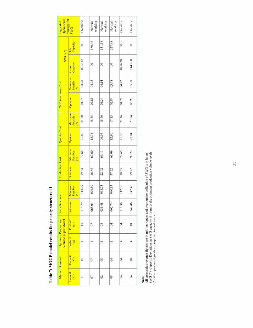
M

arke

t Dem

and

Opt

imum

Pro

duct

ion

Vol

ume

as p

er M

odel

Sa

les R

even

ue

Prod

uctio

n C

ost

Qua

lity

Cos

t W

IP in

vent

ory

Cos

t SW

G (*

) Pr

oduc

t1

(V1)

Prod

uct2

(V

2)

Prod

uct1

(x

1)

Prod

uct2

(x

2)

Opt

imum

M

axim

um

Poss

ible

(*

)

Opt

imum

M

axim

um

Poss

ible

(*

)

Opt

imum

M

axim

um

Poss

ible

(*

)

Opt

imum

M

axim

um

Poss

ible

(*

)

Ove

r-

Cap

acity

Idle

C

apac

ity

Sugg

este

d O

pera

tiona

l St

rate

gy fo

r SW

G

11

15

11

15

113.

79

113.

79

79.6

4 79

.64

21.6

0 21

.60

04.7

8 04

.78

0212

.12

00

Ove

rtim

e

07

07

11

07

065.

04

096.

59

46.8

5 67

.60

12.7

1 18

.35

02.8

1 04

.05

00

180.

68

Nor

mal

w

orki

ng

02

08

11

08

031.

48

098.

73

22.4

2 69

.11

06.0

7 18

.76

01.3

4 04

.14

00

131.

58

Nor

mal

w

orki

ng

08

04

11

04

065.

74

090.

13

47.5

2 63

.09

12.9

0 17

.13

02.8

4 03

.78

00

327.

98

Nor

mal

w

orki

ng

14

04

14

04

112.

36

112.

36

78.6

5 78

.65

21.3

6 21

.36

04.7

2 04

.72

0756

.28

00

Ove

rtim

e

14

18

14

18

142.

46

142.

46

99.7

2 99

.72

27.0

4 27

.04

05.9

8 05

.98

1443

.68

00

Ove

rtim

e

Not

e:

All

cost

s/sa

les r

even

ue fi

gure

s are

in m

illio

n ru

pees

and

ove

r /un

der u

tiliz

atio

n of

SW

G is

in h

ours

SW

G (*

): C

apac

ity D

evia

tions

in S

WG

cap

acity

if it

runs

at t

he o

ptim

um p

rodu

ctio

n vo

lum

e le

vels

(*

): if

all p

rodu

ced

good

s are

supp

lied

to c

usto

mer

s

36

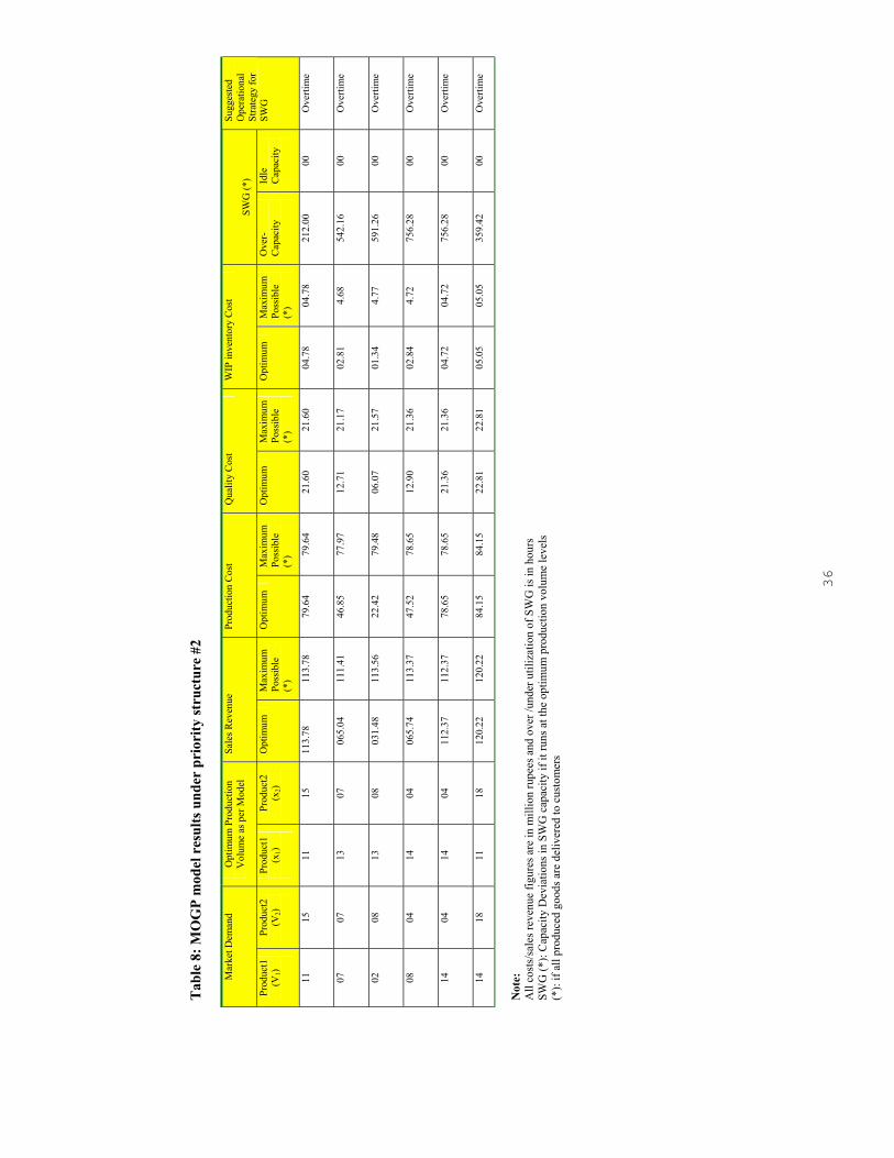
Tab

le 8

: MO

GP

mod

el r

esul

ts u

nder

pri

ority

stru

ctur

e #2

Mar

ket D

eman

d O

ptim

um P

rodu

ctio

n V

olum

e as

per

Mod

el

Sale

s Rev

enue

Pr

oduc

tion

Cos

t Q

ualit

y C

ost

WIP

inve

ntor

y C

ost

SWG

(*)

Prod

uct1

(V

1)

Prod

uct2

(V

2)

Prod

uct1

(x

1)

Prod

uct2

(x

2)

Opt

imum

M

axim

um

Poss

ible

(*

)

Opt

imum

M

axim

um

Poss

ible

(*

)

Opt

imum

M

axim

um

Poss

ible

(*

)

Opt

imum

M

axim

um

Poss

ible

(*

)

Ove

r-

Cap

acity

Idle

C

apac

ity

Sugg

este

d O

pera

tiona

l St

rate

gy fo

r SW

G

11

15

11

15

113.

78

113.

78

79.6

4 79

.64

21.6

0 21

.60

04.7

8 04

.78

212.

00

00

Ove

rtim

e

07

07

13

07

065.

04

111.

41

46.8

5 77

.97

12.7

1 21

.17

02.8

1 4.

68

542.

16

00

Ove

rtim

e

02

08

13

08

031.

48

113.

56

22.4

2 79

.48

06.0

7 21

.57

01.3

4 4.

77

591.

26

00

Ove

rtim

e

08

04

14

04

065.

74

113.

37

47.5

2 78

.65

12.9

0 21

.36

02.8

4 4.

72

756.

28

00

Ove

rtim

e

14

04

14

04

112.

37

112.

37

78.6

5 78

.65

21.3

6 21

.36

04.7

2 04

.72

756.

28

00

Ove

rtim

e

14

18

11

18

120.

22

120.

22

84.1

5 84

.15

22.8

1 22

.81

05.0

5 05

.05

359.

42

00

Ove

rtim

e

Not

e:

All

cost

s/sa

les r

even

ue fi

gure

s are

in m

illio

n ru

pees

and

ove

r /un

der u

tiliz

atio

n of

SW

G is

in h

ours

SW

G (*

): C

apac

ity D

evia

tions

in S

WG

cap

acity

if it

runs

at t

he o

ptim

um p

rodu

ctio

n vo

lum

e le

vels

(*

): if

all p

rodu

ced

good

s are

del

iver

ed to

cus

tom

ers

37

Also for both the cases, the associated costs such as production, quality and WIP

inventory are summarized in Table 7. To gain more insights from the proposed

MOGP approach, select the following optimal solution from Table 5 for the

product scenario (14,18):

x1 = 14, x2 = 18,

d2- = d2

+ = d3- = d3

+ = d4- = d6

- = 0, d1+ = 27.04, d5

+ = 78.65, d7+ = 5.98.

The goals such as product volumes under priority1 and sales revenue under

priority3 are achieved, but the other goals such as quality cost, production cost,

and WIP inventory are not completely minimized. This kind of result reflects a

typical day to day production situation where there are several minimum costs

while producing some tangible goods. The associated quality, production, and

WIP inventory costs incurred for production of 14 CNC machining centres and 18

CNC lathes in the year are 99.72, 27.04, and 5.98 million rupees respectively. To

get further clarity of the proposed MOGP model, the result under product volume

scenario (11,15) is also now analyzed. The solution of the problem yields the

following results at this scenario.

(a). Variables: x1 = 11, x2 = 15, d2- = d2

+ = d3- = d3

+ = d6- = 0;

d1+ = 21.60, d5

+ = 79.64, d6+ = 212.12, d7

+ = 4.78.

The solution indicates that the firm produces 11 CNC machining centres and 15

CNC lathes with 212.12 hours of overtime operation in SWG machine. The total

sales revenue was 113.79 million rupees (refer Table 5), 1.21 million rupees (i.e.

d-4, refer Table 7) short of the 115 million rupees limit as set be the management.

The associated costs of quality, production, and WIP inventory in the particular

year are 21.60, 79.64, 4.78 million rupees respectively. The revenue and cost

38

figures will facilitate the management for allocation of budget to the concern

departments to meet the various activities of production.

(b) Goal attainment

Product1 volume goal: Achieved

Product2 volume goal: Achieved

Avoid underutilization utilization of SWG goal: Achieved

Sale revenue goal: Not achieved

The above-stated goal attainments indicate that the firm is able to achieve the

goals of market and the most important manufacturing process related goal (i.e.

avoid underutilization of SWG) during the year. The optimal solution is to avoid

product shortages and underutilization of the normal production capacity of the

SWG by scheduling overtime operation whenever this is possible. In this way our

MOGP model results will act as an effective communication tool between the top

and lower level managers of the case study to enhance the productivity of the

system as well as for improvement of the business However, under this goal

priority structure #1 some of our critical observations are as follows:

• The organization may closely meet the sales revenue target of 115

million rupees if it decide to produce product volume combinations

either (11, 15) or (14, 4). However, this can be achieved at the expense

of additional operational cost especially due to overtime operational

strategy of SWG (refer Table 7).

• As explained in the problem context, SWG is only the bottleneck

machine. Goal deviations with respect to this machine are also presented

in Table 5. Results indicate that SWG machine will be under-utilized if

the product demands are (7, 7), (2,8) and (8,4) for instance. Whereas for

39

other scenarios of product demands the machine capacity of SWG is

insufficient under normal working conditions. To operationalize the

solution, the company should run the SWG on overtime basis

(according to over utilized hours prescribed by the model) to meet the

on time delivery of products to the market. The suggested operational

strategy for SWG under each of the product scenario is also summarized

in Table 7. This information facilitates the planner specifically to tackle

the issue of workforce balancing i.e. to maintain good employer-

employee relations on long term basis, indeed it was one of the main

objective of the management of the firm under consideration.

Priority structure #2

Under the priority structure #2, the first priority i.e. meet product2 demand goal

was fully satisfied in all product scenarios. The product1 demand goal, which was

assigned as the second priority was satisfied only in the two occasions i.e. at

(11,15) and (14,4) product scenarios. Further, at the product scenario of (14,18), it

is not only to meet the sales revenue goal, which was kept as a second priority but

also to cross the sales revenue target of 113 million rupees. The goal in that case

was to maintain product1 demand level of 14 and was included under priority 2

i.e. P2. However, there is a shortage of 3 units in the product1 demand that

represents a curtailment of product1 production, resulting underachievement of

this goal (d2- = 3, refer Table 6). In this case the company does not prefer this

production strategy. In priority structure #2 also, the best operational solution to

the selected firm is that of product scenario (11,15), at which it can meet the sales

40

revenue limit with a slight higher margin of 0.78 million rupees (Table 8) as well

as product1 and product2 demand goals.

The optimal production volumes at production scenarios (11,15) and

(14,4) are the only production volume levels that coincide with the priority

structure #1 solution. Therefore, the maximum possible measures such as sales

revenue, production cost, quality cost, and WIP inventory are realized in product

scenarios (11,15) and (14,4) are the same under both the priority structure #1 and

the priority structure #2 solution. The only difference between the two solutions

occurs in the suggested operational strategy of SWG due to deviations (cf. last

column of Table 7 and 8) in its capacity at various product scenarios as stipulated

by the marketing managers.

The results of the priority structure #1 are compared with the priority

structure #2 for the same planning period. The trade-offs between the two

solutions is evident: in the priority structure #2, variations such as costs were high

if the company wants to sell/supply all the produced goods. To operationalize a

solution where the xi�s do not equal to �goal product demand� marketing

department seeks, it may be advisable to look for the ways to increase the product

sales perhaps through sales promotion schemes. Otherwise costs such as

production, quality and WIP inventory will be increased enormously when

compared with priority structure #1 values. For example for the product scenario

(7,7), the cost changes are: production cost from 67.61 to 77.97 million rupees,

quality costs 18.35 to 21.17 million rupees, and WIP inventory 4.05 to 4.68

million rupees. Although various costs are increasing, the customer

satisfaction in terms of offering better quality products outweighs the

41

disadvantage of increasing various costs. Even more important than

savings in costs is the achievement of marketing goal, i.e. nothing but

timely supply of products to the customers, which is the key policy of the

company in running its business in a competitive manner. Except in one

product scenario, i.e. under priority structure #2, this can be seen from

Table 5 and Table 6, where the underachievement in product demand goals

tends to zero. Also, It can be seen from the results that the WIP inventory cost

decreases substantially for the priority structure #1 in all the product scenarios,

thus satisfying the main objective of the company and hence the results obtained

under this priority structure are recommended to the case organization for further

consideration.

From the results of MOGP model, it can be seen that the model performs

well in communicating the trade-offs among the various performance measures to

various functional levels of the organization such as marketing, sales, finance and

operations. These cost figures are useful for these departments for routine

planning and scheduling. In both of the priority structures, there are some

instances when the product demand goals have crossed the targets, resulting in the

higher costs. But these instances are found to be rare, and at the most seen in three

occasions of product scenarios. However, the overachivements are not serious as,

in any way, the information can be used as a basis to arrive to an appropriate

production plan.

42

5 Summary, Conclusions, and Further Research

Summary

Development of goal programming models and their applications to the real life

manufacturing problems have received an increasing attention during the past

several years as a powerful decision making tool for the problems that involve

multiple conflicting objectives. Modern manufacturing is complex owing to

increased uncertainty in the customer demands, competitive markets, and rapid

technological developments. Production management under this scenario is

challenging and the problem complexity is due to some of the following features:

• The product structures looks similar but are not identical.

• The operational capacities are the only constraints from the system view.

• Product demand is highly uncertain.

In such a scenario, it is necessary to determine the optimum production

plan to assist the decision maker to achieve the organization goals for optimum

utilization of resources. The MOGP model presented in this paper would be useful

to discrete item manufacturers especially to find out an optimum level of

production activities in terms of utilization of the critical machine i.e. SWG.

The MOGP results of the study are of significance to the production

manager in decision making for long run production planning and scheduling of

SWG operation. Also it can be useful to other functional areas such as marketing

and finance for routine planning. Some of the specific decision making situations

in this context are-

(i). the expected quality costs and production costs under identified product

scenarios

43

(ii). under and over utilization of SWG at different combinations of production

volumes

(iii). the achievement of sales revenue goal at different production volume

combinations

These results are expected to guide the production manager to estimate

the effects of product mix changes on load conditions at SWG. In this way, the

MOGP output may act as a link between the firm�s broad strategies and tactical

plans that enable the firm to achieve its goals. However, the three entities

customer, manufacturer, and competitor must weigh the consequences of

accomplishing goals at the expense of others and must attain acceptable balance in

the achievement of their various goals.

Conclusions

The paper investigates the MOGP approach when applied to a real life case

situation with an intention to evaluate the trade-offs of the three entities of the

production planning environment under multiple conflicting objectives. To

simplify this illustration, the problem was limited in a scope to an application of

only one division of the case study. However, an application such as this could be

easily be expanded to deal with the more complex real world problems

confronting planners and managers. We notice that results show that the model

can be an effective planning tool to aid decision makers faced with multiple

conflicting goals where the three entities of production planning are significant

determiners of any firm�s success. In addition, the model is computationally

feasible, it requires approximately a three seconds to obtain the results for the

selected data.

44

Further research In the proposed MOGP approach, all of the parameters are assumed as

constants and deterministic. In other words, the problem requires a solution in a

static decision environment. However, in reality the decision environment is

usually dynamic rather than static. Therefore, the model coefficients are neither

known nor constant. Hence, some research efforts concerning stochastic

approach are needed in this regard. Also, We recommend the use of regression

analysis for estimation of various parameters and to more accurately weight the

importance of various performance measures such as quality, production

overheads, and WIP inventory. Lastly but not least, we also encourage

researchers to explore the use of AHP for determining relative weights or

priorities based on numerous qualitative factors, where AHP may bring a

recognized and uniformly fair framework for the assessment of those weights.

References: Agarwal, V. P., Kohli, V., and Gupta, S. (1991), Computer aided robot selection: the multiple attribute decision making approach, International Journal of Production Research, Vol.29, No. 8, pp.1629-1644.

Aouni, B. and Kettani, O. (2001), Goal programming model: a glorious history and a promising future, European Journal of Operational Research, Vol. 133, pp. 225-231. Atmani, A. (1995), A production planning model for flexible manufacturing systems with setup cost consideration, Computers and Industrial Engineering Journal, Vol. 29, No. 1-4, pp. 723-727. Buzacott, J. A. and Shanthikumar, J. G. (1993), Stochastic Models of

Manufacturing Systems, Prentice Hall, New Jersey. Charnes, A. and Cooper, W. W. (1961), Management Models and Industrial Application of Linear Programming, Vol. 1, Wiley, New York.

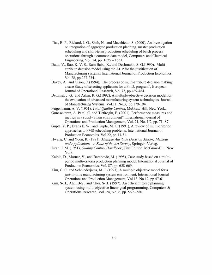
45

Das, B. P., Rickard, J. G., Shah, N., and Macchietto, S. (2000), An investigation on integration of aggregate production planning, master production scheduling and short-term production scheduling of batch process

operations through a common data model, Computers and Chemical Engineering, Vol. 24, pp. 1625 � 1631. Datta, V., Rao, K. V. S., Ram Babu, K., and Deshmukh, S. G.(1990), Multi- attribute decision model using the AHP for the justification of Manufacturing systems, International Journal of Production Economics, Vol.28, pp.227-234. Davey, A. and Olson, D.(1994), The process of multi-attribute decision making: a case Study of selecting applicants for a Ph.D. program�, European Journal of Operational Research, Vol.72, pp.469-484. Demmel, J. G. and Askin, R. G.(1992), A multiple-objective decision model for the evaluation of advanced manufacturing system technologies, Journal of Manufacturing Systems, Vol.11, No.3, pp.179-194. Feigenbaum, A. V. (1961), Total Quality Control, McGraw-Hill, New York. Gunasekaran, A. Patel, C. and Tirtiroglu, E. (2001), Performance measures and metrics in a supply chain environment�, International journal of Operations and Production Management, Vol. 21, No. 1/2, pp. 71- 87.

Gupta, Y. P., Evans E. W., and Gupta, M. C. (1991), A review of multi-criterion approaches to FMS scheduling problems, International Journal of Production Economics, Vol.22, pp.13-31. Hwang, C. and Yoon, K. (1981), Multiple Attribute Decision Making Methods and Applications - A State of the Art Survey, Springer- Verlag. Juran, J. M. (1951), Quality Control Handbook, First Edition, McGraw-Hill, New York. Kalpic, D., Mornar, V., and Baranovic, M. (1995), Case study based on a multi- period multi-criteria production planning model, International Journal of Production Economics, Vol. 87, pp. 658-669. Kim, G. C. and Schniederjams, M. J. (1993), A multiple objective model for a just-in-time manufacturing system environment, International Journal Operations and Production Management, Vol.13, No.12, pp.47-61. Kim, S-H., Ahn, B-S., and Choi, S-H. (1997), An efficient force planning system using multi-objective linear goal programming, Computers & Operations Research, Vol. 24, No. 6, pp. 569 �580.

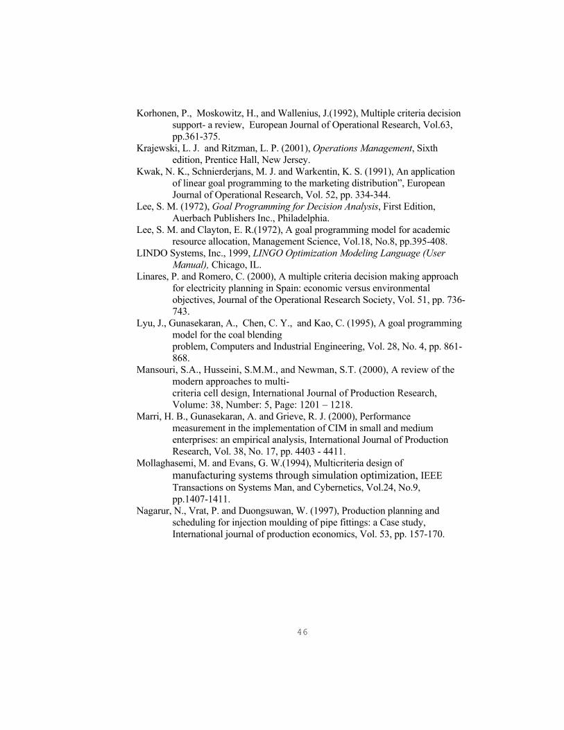
46

Korhonen, P., Moskowitz, H., and Wallenius, J.(1992), Multiple criteria decision support- a review, European Journal of Operational Research, Vol.63, pp.361-375. Krajewski, L. J. and Ritzman, L. P. (2001), Operations Management, Sixth edition, Prentice Hall, New Jersey. Kwak, N. K., Schnierderjans, M. J. and Warkentin, K. S. (1991), An application

of linear goal programming to the marketing distribution�, European Journal of Operational Research, Vol. 52, pp. 334-344.

Lee, S. M. (1972), Goal Programming for Decision Analysis, First Edition, Auerbach Publishers Inc., Philadelphia. Lee, S. M. and Clayton, E. R.(1972), A goal programming model for academic

resource allocation, Management Science, Vol.18, No.8, pp.395-408. LINDO Systems, Inc., 1999, LINGO Optimization Modeling Language (User Manual), Chicago, IL. Linares, P. and Romero, C. (2000), A multiple criteria decision making approach for electricity planning in Spain: economic versus environmental objectives, Journal of the Operational Research Society, Vol. 51, pp. 736- 743. Lyu, J., Gunasekaran, A., Chen, C. Y., and Kao, C. (1995), A goal programming model for the coal blending problem, Computers and Industrial Engineering, Vol. 28, No. 4, pp. 861- 868. Mansouri, S.A., Husseini, S.M.M., and Newman, S.T. (2000), A review of the

modern approaches to multi- criteria cell design, International Journal of Production Research, Volume: 38, Number: 5, Page: 1201 � 1218.

Marri, H. B., Gunasekaran, A. and Grieve, R. J. (2000), Performance measurement in the implementation of CIM in small and medium enterprises: an empirical analysis, International Journal of Production Research, Vol. 38, No. 17, pp. 4403 - 4411. Mollaghasemi, M. and Evans, G. W.(1994), Multicriteria design of manufacturing systems through simulation optimization, IEEE Transactions on Systems Man, and Cybernetics, Vol.24, No.9, pp.1407-1411.

Nagarur, N., Vrat, P. and Duongsuwan, W. (1997), Production planning and scheduling for injection moulding of pipe fittings: a Case study, International journal of production economics, Vol. 53, pp. 157-170.

47

Olhager, J. and Wikner, J. (2000), Production planning and control tools, Production Planning and Control, Vol. 11, No. 3, pp. 210-222.

Ozdamar, L., Bozyel, M. A., and Birbil, S. I. (1998), A hierarchical decision support system for production planning (with case study), European Journal of Operational Research, Vol. 104, pp. 403-422. Premchandra, I. M. (1993), A goal programming model for activity crashing in project networks, International Journal of Operations and Production Management, Vol.13, No.6, pp. 79-85. Ravindran, P.(1987), Operations Research Principles and Practice, John Wiley and Sons Inc., New York. Romero, C. (1990), Handbook of Critical Issues in Goal Programming, Pergamon Press, New York. Romero, C. G. (1986), A survey of generalized goal programming (1970-1982), European Journal of Operational Research, Vol. 25, pp. 183-191. Schniederjans, M. J. (1995), Goal Programming Methodology and Applications, Kluwer Academic Publishers, Boston. Schniederjans, M. J. and Hoffman, J. J. (1992), Multinational acquisition analysis: A zero-one goal programming model, European Journal of Operational Research, Vol. 62, No. 2, pp. 175 -185. Shafer, S. M., and Rogers, D. F. (1991), A goal programming approach to the cell formation problem, Journal of Operations Management, Vol. 10, No. 1, pp.28-43. Shang, J. S. and Tadikamalla, P. R. (1998), Multicriteria design and control of a cellular manufacturing system through simulation and optimization, International Journal of Production Research, Vol.36, No.6, pp.1515-1528. Singh, N. and Agarwal, S. K. (1983), Optimum design of an extended octogonal ring by goal programming, International Journal of Production Research, Vol.21, No.6, pp.891-898. Slack, N., Chambers, S., Harland, C., Harrison, A. and Johnston, R. (2000), Operations Management, Pitman Publishing, London. Son, Y. K. and Park, C. S. (1987), Economic measure of productivity, quality and flexibility in advanced manufacturing systems, Journal of Manufacturing Systems, Vol.6, No.3, pp. 193-207. Son, Y. K. (1993), Simulation-based manufacturing accounting for modern management, Journal of Manufacturing Systems, Vol.12, No. 5, pp. 417 � 427.

48

Stam, A. and Kuula, M.(1991), Selecting a flexible manufacturing system using multiple criteria analysis, International Journal of Production Research, Vol.29, No.4, pp. 803-820. Steuer, R. E. (1985), Multiple-criteria optimization: Theory, Computation and Application, John Wiley and Sons. Stewart, T. J. (1992), A critical survey on the status of multiple criteria decision making - theory and practice, OMEGA International Journal of Management Science, Vol.20, No.5/6, pp. 569-586. Su, C. T. and Hsu, C. M. (1998), Multi-objective machine-part cell formation through parallel simulated annealing, International Journal of Production Research, Vol. 36, No. 8, pp.2185 � 2207. Sundaram, R. M. (1978), An application of goal programming technique in metal cutting, International Journal of Production Research, Vol.16, No.5, pp. 375-382. Tabucanon, M. T. and Majumdar, S. (1989), Production Planing in a Ship Repair Company in Bangladesh, Proceedings of the International Conference on MCDM: Applications in Industry and Service, Asian

Institute of Technology, Bangkok, pp. 47-61. Tamiz, M., Jones, D., and Romero, C. (1998), Goal programming for decision

making: An overview of the current state-of-the-art, European Journal of Operational Research, Vol. 111, pp. 569-581.

Viswanadham, N. and Narahari, Y. (1994), Performance Modeling of Automated Manufacturing Systems, Prentice-Hall of India private Ltd., New Delhi.

Wang, T. Y., Shaw, C. F. and Chen, Y. L. (2000), Machine selection in flexible manufacturing cell: a fuzzy multiple attribute decision-making approach, International Journal of Production Research, Vol. 38, No. 9, pp. 2079 - 2097.

Zhao, C. and Wu, Z. (2000), A genetic algorithm for manufacturing cell formation with multiple routes and multiple objectives, International Journal of Production Research, Vol. 38, No. 2, pp. 385 - 395.