


Languages
Pages
Legal


A METHODOLOGY TO DETERMINE BOTH THE TECHNICALLY
RECOVERABLE RESOURCE AND THE ECONOMICALLY RECOVERABLE
RESOURCE IN AN UNCONVENTIONAL GAS PLAY
A Thesis
by
HUSAMEDDIN SALEH A. ALMADANI
Submitted to the Office of Graduate Studies of Texas A&M University
in partial fulfillment of the requirements for the degree of
MASTER OF SCIENCE
August 2010
Major Subject: Petroleum Engineering

A METHODOLOGY TO DETERMINE BOTH THE TECHNICALLY
RECOVERABLE RESOURCE AND THE ECONOMICALLY RECOVERABLE
RESOURCE IN AN UNCONVENTIONAL GAS PLAY
A Thesis
by
HUSAMEDDIN SALEH A. ALMADANI
Submitted to the Office of Graduate Studies of Texas A&M University
in partial fulfillment of the requirements for the degree of
MASTER OF SCIENCE
Approved by:
Chair of Committee, Stephen A. Holditch
Committee Members, Walter B. Ayers Julian E. Gaspar Head of Department, Stephen A. Holditch
August 2010
Major Subject: Petroleum Engineering

iii
ABSTRACT
A Methodology to Determine both the Technically Recoverable Resource and the
Economically Recoverable Resource in an Unconventional Gas Play.
(August 2010)
Husameddin Saleh A. AlMadani, B.S., University of Kansas
Chair of Advisory Committee: Dr. Stephen A. Holditch
During the past decade, the worldwide demand for energy has continued to
increase at a rapid rate. Natural gas has emerged as a primary source of US energy. The
technically recoverable natural gas resources in the United States have increased from
approximately 1,400 trillion cubic feet (Tcf) to approximately 2,100 trillion cubic feet
(Tcf) in 2010. The recent declines in gas prices have created short-term uncertainties and
increased the risk of developing natural gas fields, rendering a substantial portion of this
resource uneconomical at current gas prices.
This research quantifies the impact of changes in finding and development costs
(F&DC), lease operating expenses (LOE), and gas prices, in the estimation of the
economically recoverable gas for unconventional plays. To develop our methodology,
we have performed an extensive economic analysis using data from the Barnett Shale, as
a representative case study. We have used the cumulative distribution function (CDF) of
the values of the Estimated Ultimate Recovery (EUR) for all the wells in a given gas
play, to determine the values of the P10 (10th percentile), P50 (50th percentile), and P90

iv
(90th percentile) from the CDF. We then use these probability values to calculate the
technically recoverable resource (TRR) for the play, and determine the economically
recoverable resource (ERR) as a function of F&DC, LOE, and gas price. Our selected
investment hurdle for a development project is a 20% rate of return and a payout of 5
years or less. Using our methodology, we have developed software to solve the problem.
For the Barnett Shale data, at a F&DC of $3 Million, we have found that 90% of the
Barnet shale gas is economically recoverable at a gas price of $46/Mcf, 50% of the
Barnet shale gas is economically recoverable at a gas price of $9.2/Mcf, and 10% of the
Barnet shale gas is economically recoverable at a gas price of $5.2/Mcf. The developed
methodology and software can be used to analyze other unconventional gas plays to
reduce short-term uncertainties and determine the values of F&DC and gas prices that
are required to recover economically a certain percentage of TRR.

v
DEDICATION
To Dr. Ghazi AlQusaibi who has, unknowingly, inspired entire generations of positive
citizens and change agents in Saudi Arabia throughout
his life commitment and long years of
dedicated public
service.
To the late Eng. Bandar AlAnazi, who, during his very short life
on earth, carried an inspiring passion
for engineering, knowledge sharing,
and community
service.

vi
ACKNOWLEDGEMENTS
This thesis would not have been possible without the guidance and support from
my committee chair, Dr. Stephen Holditch, throughout the course of research. I am
indebted to his distinctive knowledge and ability to challenge me while providing the
essential supervision to ensure the fruition of this research. I would also like to thank Mr.
George Voneiff with Unconventional Gas Resources, LLC, and Mr. William D. Von
Gonten, Jr. with WD Von Gonten & Company for providing datasets and feedback to
calibrate my research findings.
My sincere thanks also go to my advisory committee members, Dr. Walter B.
Ayers and Dr. Julian E. Gaspar for their critical feedback, significant input, and
mentorship during this journey. Their confidence in my ability to conduct this research
has always inspired me to rise to the challenge.
I would also like to express my gratitude to my wife, Anat AlMadani, for her
patience, love and support. She has always been there for me, and for that, I am most
grateful.
Finally, I would like to express my sincere appreciation to Saudi ARAMCO, for
sponsoring my graduate school and for providing its employees with unprecedented
development resources to be the best employes and citizens they can be. I am truly proud
to be associated with a company with unrivaled commitment to maintain its world-
leading role as a reliable energy provider to the globe while developing and nurturing the
future generations of engineers and leaders of Saudi Arabia.

vii
NOMENCLATURE
Bcf billion cubic feet
CBM coalbed methane
CDF cumulative distribution function
DOE Department of Energy
EIA Energy Information Administration
ERR economically recoverable resource
EUR estimated ultimate recovery
F&DC finding and development cost
LOE lease operating expenses
Mcf million cubic feet
Mcfe million cubic feet equivalent
OGIP original gas in place
P(EUR) cumulative distribution function of EURs
P10 10% probability of occurrence
P50 50% probability of occurrence
P90 90% probability of occurrence
P10 Well a well with a 90% chance of EUR similar to or higher than the
10th percentile
P50 Well a well with a 50% chance of a higher EUR and a 50% chance of
less EUR than the 50th percentile
viii
P90 Well a well with a 10% chance of EUR that is higher than the 90th
percentile
P* Well a well with a weighted EUR based on P10, P50, and P90 EUR
values
ROR rate of return
Tcf trillion cubic feet
TRR technically recoverable resource
UG unconventional gas
USGS US Geological Survey
VBA Visual Basic Application

ix
TABLE OF CONTENTS
Page
ABSTRACT ................................................................................................................. iii
DEDICATION............................................................................................................... v
ACKNOWLEDGEMENTS .......................................................................................... vi
NOMENCLATURE .................................................................................................... vii
TABLE OF CONTENTS .............................................................................................. ix
LIST OF TABLES ....................................................................................................... xii
LIST OF FIGURES .................................................................................................... xiv
1 INTRODUCTION .................................................................................................. 1
1.1 The Natural Gas Resource Base...................................................................... 4
1.2 Technically Recoverable Resources ................................................................ 6
1.3 Economically Recoverable Resources ............................................................ 7
1.4 Estimated Ultimate Recovery (EUR) .............................................................. 8
1.5 Significance of Unconventional Gas Development ....................................... 10
2 THE QUESTION AND OBJECTIVES ................................................................ 13
3 PROCEDURE ...................................................................................................... 14
3.1 Literature Review ......................................................................................... 14
3.2 Case Study ................................................................................................... 14
4 FACTORS AFFECTING THE ESTIMATION OF ECONOMICALLY
RECOVERABLE GAS RESOURCES ................................................................. 15
4.1 Finding and Development Cost..................................................................... 15

x
Page
4.2 Lease and Operating Expenses ..................................................................... 16
4.3 Gas Prices .................................................................................................... 17
4.3.1 The Price Cycle ................................................................................... 18
4.3.2 The Effect of Weather ......................................................................... 19
4.3.3 Economic Activity ............................................................................... 20
4.3.4 Underground Storage ........................................................................... 20
4.3.5 Oil Prices............................................................................................. 21
5 INVESTMENT HURDLE: WHAT IS ECONOMICAL? ...................................... 22
5.1 Abundant Resources ..................................................................................... 22
5.2 Investment Hurdle Criteria ........................................................................... 24
6 CASE STUDY: THE BARNETT SHALE ............................................................ 25
6.1 The Barnett Shale: A Hot Play ...................................................................... 25
6.2 Barnett Shale Production Profile ................................................................... 29
6.3 Production Forecast Using Hyperbolic Decline Curves ................................. 30
7 ECONOMIC ANALYSIS..................................................................................... 37
7.1 Well-Level Economics: Scenario I ............................................................... 37
7.1.1 Economics for P10, P50, P90 Wells at Scenario I ................................ 37
7.1.2 Economics forP* Well at Scenario I .................................................... 43
7.2 Well-Level Economics: Scenario II .............................................................. 47
7.2.1 Economics for P10, P50, P90, and P* Wells at Scenario II................... 48
7.3 Determining TRR from a P* Well ................................................................ 55
7.4 Sensitivity Analysis ...................................................................................... 56
7.5 Economic Analysis at Every Percentile ........................................................ 59
8 DISCUSSION OF RESULTS ............................................................................... 64
9 CONCLUSIONS AND RECOMMENDATIONS ................................................. 69
REFERENCES ............................................................................................................ 72
APPENDIX A ............................................................................................................. 75

xi
Page
APPENDIX B .............................................................................................................. 76
APPENDIX C .............................................................................................................. 77
VITA ........................................................................................................................... 85
xii
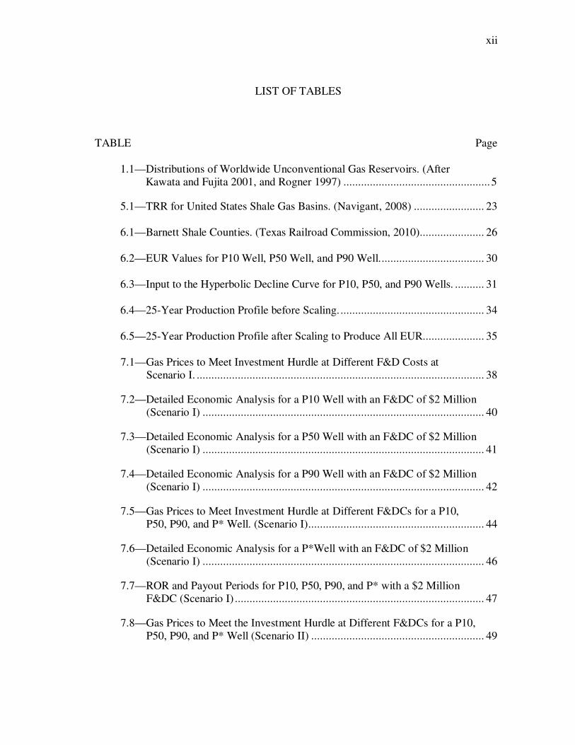
LIST OF TABLES
TABLE Page
1.1—Distributions of Worldwide Unconventional Gas Reservoirs. (After Kawata and Fujita 2001, and Rogner 1997) .................................................. 5
5.1—TRR for United States Shale Gas Basins. (Navigant, 2008) ........................ 23
6.1—Barnett Shale Counties. (Texas Railroad Commission, 2010)...................... 26
6.2—EUR Values for P10 Well, P50 Well, and P90 Well. ................................... 30
6.3—Input to the Hyperbolic Decline Curve for P10, P50, and P90 Wells. .......... 31
6.4—25-Year Production Profile before Scaling. ................................................. 34
6.5—25-Year Production Profile after Scaling to Produce All EUR..................... 35
7.1—Gas Prices to Meet Investment Hurdle at Different F&D Costs at Scenario I. .................................................................................................. 38
7.2—Detailed Economic Analysis for a P10 Well with an F&DC of $2 Million (Scenario I) ................................................................................................ 40
7.3—Detailed Economic Analysis for a P50 Well with an F&DC of $2 Million (Scenario I) ................................................................................................ 41
7.4—Detailed Economic Analysis for a P90 Well with an F&DC of $2 Million (Scenario I) ................................................................................................ 42
7.5—Gas Prices to Meet Investment Hurdle at Different F&DCs for a P10, P50, P90, and P* Well. (Scenario I) ............................................................ 44
7.6—Detailed Economic Analysis for a P*Well with an F&DC of $2 Million (Scenario I) ................................................................................................ 46
7.7—ROR and Payout Periods for P10, P50, P90, and P* with a $2 Million F&DC (Scenario I) ..................................................................................... 47
7.8—Gas Prices to Meet the Investment Hurdle at Different F&DCs for a P10, P50, P90, and P* Well (Scenario II) ........................................................... 49
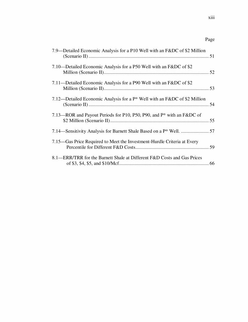
xiii
Page
7.9—Detailed Economic Analysis for a P10 Well with an F&DC of $2 Million (Scenario II) ............................................................................................... 51
7.10—Detailed Economic Analysis for a P50 Well with an F&DC of $2 Million (Scenario II) ................................................................................... 52
7.11—Detailed Economic Analysis for a P90 Well with an F&DC of $2 Million (Scenario II) ................................................................................... 53
7.12—Detailed Economic Analysis for a P* Well with an F&DC of $2 Million (Scenario II) ............................................................................................... 54
7.13—ROR and Payout Periods for P10, P50, P90, and P* with an F&DC of $2 Million (Scenario II) .............................................................................. 55
7.14—Sensitivity Analysis for Barnett Shale Based on a P* Well. ...................... 57
7.15—Gas Price Required to Meet the Investment-Hurdle Criteria at Every Percentile for Different F&D Costs .......................................................... 59
8.1—ERR/TRR for the Barnett Shale at Different F&D Costs and Gas Prices of $3, $4, $5, and $10/Mcf ....................................................................... 66

xiv
LIST OF FIGURES
FIGURE Page
1.1—Impact of Technology and Economic Conditions on Gas Recovery. ............ 3
1.2—Resource Triangle for Natural Gas. (Holditch, 2006) ................................... 4
1.3—Growth of US Technically Recoverable Natural Gas Resources. (EIA, 2010b) ........................................................................................................ 7
1.4—EIA Resource Classification and Organization. (EIA) ................................. 8
1.5—Oil, Gas, and Water Production Data from a Well in a an Unconventional Resource. (Cook, 2005) ..................................................... 9
1.6—Example of an EUR distribution for 4000 Wells in an Unconventional Gas Resource. ................................................................ 10
1.7—Forecast of Shale Gas Growth in Meeting Energy Demand. (EIA, 2010b) ..................................................................................................... 11
1.8—Unconventional Natural Gas Outlook in the US (Bcf/day). (DOE, 2009)…12
4.1—Increasing F&D Cost per BOE. (Herold, 2009) ......................................... 16
4.2—F&D Cost Vary between Regions. (Herold, 2009) ..................................... 16
4.3—2006-2010 Monthly Natural Gas Prices – Based on Henry Hub. (CME, 2010)......................................................................................................... 18
4.4—Projected Natural Gas Prices. (EIA, 2010b) ............................................... 19
4.5—Gas Prices Trail Oil Prices (EIA, 2010b) ................................................... 21
5.1—United States 25 North American Basins (Singh, 2006) ............................. 22
5.2—United States Shale Gas Basins. (DOE, 2009) ........................................... 23
6.1—Barnett Shale in the Fort Worth Basin.(DOE,2009) ................................... 25
6.2—Barnett Shale Annual Total Gas Production. (Texas Railroad Commission, 2010) ................................................................................... 28

xv
Page
6.3—Barnett Shale Well Count from 1993 through 2009. (Texas Railroad Commission, 2010) ................................................................................... 29
6.4—40-Year Production Forecast for P10, P50, and P90 Wells. ....................... 32
6.5—25-Year Production Forecast for P10, P50, P90 Wells. .............................. 33
6.6—25-Year Cumulative Production for P10, P50, and P90 Wells.................... 36
7.1—Gas Prices Required to Meet Investment Hurdle at Different F&D Costs(Scenario I) ....................................................................................... 39
7.2—Confidence Intervals for a Normal Distribution Curve ............................... 43
7.3—Gas Prices to Meet Investment Hurdle at Different F&DCs a P10, P50, P90, and P* Well(Scenario I) ................................................................... 45
7.4—Gas Prices to Meet the Investment Hurdle at Different F&D Costs a P10, P50, P90, and P* Well (Scenario II) ................................................. 50
7.5—Sensitivity Analysis Chart for Barnett Shale Based on a P* Well. .............. 58
7.6—Gas Prices To Meet the Investment-Hurdle for Each Percentile for Different F&DC ...................................................................................... 63
8.1—Required Gas Prices for Different F&DCs at Selected ERR/TRR .............. 65
8.2—Percentage of ERR/TRR at Different Gas Prices and Different F&DCs ..... 67
8.3—Percentage of ERR/TRR at Different Gas Prices and Different F&DCs on a Semi-Log Scale ................................................................................ 68

1
1 INTRODUCTION
With declining conventional gas reserves in the United States, unconventional
gas reservoirs are emerging as critical energy sources to meet the ever increasing demand
for energy. The US Department of Energy’s April 2009 report, “Modern Shale Gas
Development in the United States: A Primer,” stated that over the last decade, production
from unconventional resources in the US has increased almost 65%, from 5.4 trillion
cubic feet per year (Tcf/yr) in 1998 to 8.9 Tcf/yr in 2007. This increase in production
indicates that approximately 46% of today’s US total gas production comes from
unconventional resources (Navigant 2008).
The increasing reliance on unconventional resources has captured the interest of
the oil and gas industry in assessing the amount of unconventional gas that is technically
recoverable in the US and worldwide. Today, the US Geological Survey, among other
agencies, periodically assesses and provides ample information in terms of how much
gas is technically recoverable in US basins. However, due to the nature of
unconventional resources and the complexity of the analysis required to develop them,
less emphasis has been placed on quantifying the impact of the range of factors that
influence the calculation of how much gas is economically recoverable. Currently, with
the publically available production data, gas prices, and costs for US basins, there is an
opportunity to develop a methodology to estimate how much gas can be economically
recovered from the reported assessments given a range of prices and costs.
___________________ This thesis follows the style of SPE Production and Facilities.

2
An unconventional gas reservoir can be defined as a natural gas reservoir that
cannot be produced at economic flow rates or in economic volumes unless the well is
stimulated by a large hydraulic fracture treatment, a horizontal wellbore, or multilateral
wellbores (Holditch, 2006). The three most common types of unconventional gas
resources are tight sands, coalbed methane (CBM), and gas shales. Due to the very low
permeability of unconventional gas reservoirs, the cost of finding, developing, and
managing those resources are usually significantly higher than with conventional
resources. For example, the number of wells, required to economically develop an
unconventional resource is, in general, significantly higher than the number of wells
required to develop a conventional reservoir. The need for drilling more wells translates
into the need for higher investment and higher economic risk when it comes to the
management of unconventional gas reservoirs.
Technology, finding and development cost (F&DC), lease operating expenses
(LOE), and market gas prices, play significant role in determining the amount of
economically recoverable gas from the reservoir’s original gas in place (OGIP). OGIP
refers to the total volume of gas contained in a reservoir before production. Using current
technology, and disregarding costs, prices, and other investment criteria, the proportion
of OGIP that can be technically produced is called technically recoverable resources
(TRR), which is always less than the OGIP. However, with favorable economic
conditions and incentives, a portion of TRR can be economically produced and is
referred to as economically recoverable resources (ERR). Fig. 1.1 illustrates the
relationship between OGIP, TRR, and ERR.

3
According to the EIA, the estimated TRR of natural gas in the US is more than
1,744 trillion cubic feet (Tcf) (EIA, 2007). Of this 1,744 Tcf, approximately 211 Tcf is
classified as ERR. The TRR of unconventional gas accounts for 60% of the onshore
recoverable resource (Navigant, 2008).
The petroleum literature and other public databases contain estimates of OGIP
and TRR for the different US basins. In accordance with government regulations, where
SEC rules require publically traded oil and gas companies to report their proved reserves,
many ERR estimates also exist for US basins. The values of resources included in SEC
reports are computed specific gas prices, F&DC, LOE, and specific investment criteria.
In this research, we will develop a methodology to quantify and correlate the
variables that influence the calculation of ERR (mainly F&DC, LOE, and gas prices), for
unconventional gas reservoirs. We will use the methodology to estimate the ERR and
Fig. 1.1—Impact of Technology and Economic Conditions on Gas Recovery.
OGIP
Gas
Volu
me
Time
TRR
ERR

4
TRR given a range of F&DC, LOE, gas prices and specific investment criteria, using the
Barnett Shale in the Fort Worth Basin as the primary data set.
1.1 The Natural Gas Resource Base
Gas reservoirs are classified as conventional or unconventional. Conventional gas
reservoirs are characterized by high permeability with the gas stored in sands and
carbonates formations in pore spaces that are interconnected. A gas resource is generally
considered conventional if it is characterized by permeability in the millidarcy range or
higher.
Unconventional gas reservoirs are characterized by low permeability with the gas
stored in tight formations such as tight sands, coalbeds, and shale. A gas resource is
generally considered unconventional if it is characterized by permeability in the
microdarcy range (Fig. 1.2). As the permeability deceases, the economic risk of
developing the resource increases, and the investment required also increases.
Fig. 1.2—Resource Triangle for Natural Gas. (Holditch, 2006)

5
The EIA defines the total natural gas resource base as all of the gas that has ever
been trapped inside the earth, including the volumes that have already been produced.
The part of the total natural gas resource base that interests investors most, however, is
the remaining natural gas waiting to be extracted. Research indicates the existence of
large, unconventional gas reservoirs located throughout the world. Rogner (1997)
estimates that there are 9,000 Tcf of OGIP in coalbed methane, 16,000 Tcf of OGIP in
shale gas, and 7,400 Tcf of OGIP in tight gas sands around the world (Table 1.1).
Table 1.1—Distributions of Worldwide Unconventional Gas Reservoirs. (After Kawata
and Fujita 2001, and Rogner 1997)
Region Coalbed Methane
Shale Gas Tight-Sand Gas Total
(Tcf) (Tcf) (Tcf) (Tcf)
North America 3,017 3,842 1,371 8228
Latin America 39 2,117 1,293 3448
Western Europe 157 510 353 1019
Central and Eastern Europe 118 39 78 235
Former Soviet Union 3,957 627 901 5485
Middle East and North Africa 0 2,548 823 3370
Sub-Saharan Africa 39 274 784 1097
Centrally planned Asia and China 1,215 3,528 353 5094
Pacific (Organization for Economic Cooperation and
Development) 470 2313 705 3,487
Other Asia Pacific 0 314 549 862
South Asia 39 0 196 235
World 9,051 16,112 7,406 32,560
Since Rogner published his paper, the oil and gas industry has discovered
enormous volumes of natural gas in North American gas and in coalbed methane around

6
the world. It is believed that the OGIP estimates in Table 1.1 are very conservative. The
industry will be updating the values in Table 1.1 and it is expected that the values of
OGIP will increase substantially. Once the new values are estimated, it will be important
to estimate both TRR and ERR globally.
1.2 Technically Recoverable Resources
Recoverable resources are defined as the part of the total resource base that can
be extracted from the earth with current technology. Typically, we locate reservoirs
containing recoverable resources using seismic, geology, and drilling exploration wells.
Once discovered, we can quantify the technically recoverable resource. For existing
reservoirs, TRR includes all the gas that has been produced, is currently being produced,
or has yet to be produced.
Undiscovered resources consist of deposits whose exact locations have not been
identified, but whose existence seems likely because of geologic settings. Although
geologists cannot specify an exact location for a reservoir’s location, they can be
reasonably certain that these natural gas reservoirs exist in specific basins and
formations. In the US, the Department of the Interior (DOI) and the US Geological
Survey (USGS 2005) estimate how much undiscovered recoverable natural gas there is
either in the United States or in offshore areas that are under the government’s control.
The total discovered and undiscovered recoverable resources are called technically
recoverable resources (TRR). They include resources that can be recovered even when
recovery is not currently economically feasible. According to EIA (2010b), the recent

7
growth of technically recoverable natural gas resources in the US is primarily because of
growth in shale gas resources (Fig. 1.3).
Fig. 1.3—Growth of US Technically Recoverable Natural Gas Resources. (EIA,
2010b)
1.3 Economically Recoverable Resources
Those resources that have been discovered, and for which a specific reservoir
location is known, can further be broken down into those resources that are currently
economically recoverable, and those that are not currently economically recoverable.
Economically recoverable resources are natural gas resources where the extraction cost is
low enough, or gas prices are high enough, for natural gas companies to make a profit.
However, as illustrated in the resource triangle concept (Fig. 1.2), if either the gas price
increases, or the technology improves, economically unrecoverable resources may
become recoverable. This is a different category than that of technically unrecoverable
resources, because although the technology either exists or will exist, it just costs too

8
much, compared to market gas prices, for extraction to be profitable. Fig. 1.4 illustrates
the different classifications of resources as presented by EIA.
Fig. 1.4—EIA Resource Classification and Organization. (EIA)
1.4 Estimated Ultimate Recovery (EUR)
The Estimated Ultimate Recovery (EUR) refers to the quantities of petroleum
which are estimated to be potentially recoverable from an accumulation, including those
quantities that have already been produced.EUR can be calculated using different
methods. The calculation of Estimated Ultimate Recovery (EUR) from oil and gas
TRR
OGIP

9
production data of individual wells and the development of EUR distributions from all
producing wells in an assessment unit are important steps in the quantitative assessment
of continuous-type hydrocarbon resources (Cook, 2005). Unconventional gas resources
are considered continuous-type hydrocarbon resources. The method adopted by USGS
2005 is to calculate EURs for all wells that have produced in an unconventional gas
resource area, define an EUR distribution for all EURs, then use the cumulative
distribution function to estimate the EUR for potential wells in the same area.
The EUR for a producing well is calculated by analyzing its production rate for a
specific timeframe. During the analysis, the production data are plotted against time, and
a hyperbolic curve is fit through the data. The EUR is the sum of all gas that is expected
to be produced up to end of the well’s life (Fig. 1.5).
Fig. 1.5—Oil, Gas, and Water Production Data from a Well in a an Unconventional
Resource. (Cook, 2005)

10
Using the calculated EURs for all producing wells, an EUR distribution is plotted
on a semi-log graph with the EURs on the x-axis and the percentage of wells in the
subset of producing wells on the y-axis (Fig. 1.6).
Fig. 1.6 Example of an EUR distribution for 4000 Wells in an Unconventional Gas
Resource.
1.5 Significance of Unconventional Gas Development
In the US, 85% of the energy used currently comes from coal, oil, or natural gas;
22% of the total energy comes from natural gas. Some experts think the percent
contribution of natural gas to the US energy supply will be fairly constant over the next
20 years (EIA, 2007). It is also plausible that the volume of natural gas produced in the
0.03 3.74
0%
20%
40%
60%
80%
100%
-1 0 1 2 3 4 5 6 7EUR in Bcf

11
US could increase substantially in the coming decades. Natural gas from gas shales can
be used to generate more electricity or provide for transportation fuel. It will continue to
be a major contributor of energy within the US because it is both abundant and
recoverable. Shale gas will continue offsetting the decline in energy supply to meet
consumption growth (Fig. 1.7).
Fig. 1.7—Forecast of Shale Gas Growth in Meeting Energy Demand. (EIA, 2010b)
The US has more than 1,744 trillion cubic feet (Tcf) of technically recoverable
natural gas, including 211 Tcf of proved reserves (the discovered, economically
recoverable fraction of the OGIP) (EIA, 2007). Assuming that the US will continue to
produce natural gas at approximately 20 Tcf/yr, which is the same rate it was produced in
2007, the current technically recoverable resource estimate is enough natural gas to
supply the US for the next 90 years (EIA, 2007). This is a conservative estimate;
historically, analysts estimating the size of the total recoverable resource have been able

12
to increase their estimates, including estimates of unconventional gas resources, as they
have gained more knowledge about the available resources and as recovery technology
has improved.
Between 1970 and 2006, the US produced approximately 725 Tcf of gas, and
increased its natural gas reserves by 6 % (BP, 2008.). This increase in reserves was
mainly caused by advancements in technology, which meant that uneconomic volumes
of gas became economically recoverable. Experts anticipate that as the US depletes its
conventional gas reserves, more of its proved reserves will come from unconventional
natural gas reservoirs. Since production from unconventional sources throughout the last
decade has increased almost 65%, from 5.4 trillion cubic feet per year (Tcf/yr) in 1998 to
8.9 Tcf/yr in 2007, this means that 46% of total US production now comes from
unconventional production (Navigant, 2008.). Fig. 1.8 illustrates the forecasted increase
daily production of unconventional in the U.S (DOE,2009).
Fig. 1.8—Unconventional Natural Gas Outlook in the US (Bcf/day). (DOE, 2009)
13
2 THE QUESTION AND OBJECTIVES
The objective of this research is to develop a methodology to quantify the impact
of changes in the finding and development costs, lease operating expenses, and gas
prices when estimating the economically recoverable resources (ERR) for
unconventional gas plays. The methodology can be applied to rapidly determine the
economically recoverable gas in unconventional resources given a range of prices
F&DC, and LOE. Primarily, the question being answered in this research is:
“Knowing the volume of technically recoverable resource (TRR) in an
unconventional gas play, how is the volume of economically recoverable resource
(ERR) affected by changes in F&DC, LOE, and gas prices?”
More specifically, our goals for this research are:
• To develop a method to compute the economically recoverable resource
in an unconventional gas reservoir;
• To apply the methodology to the Barnett Shale in North Texas and
• To illustrate how the ERR can be estimated as a function of finding and
development costs, gas prices and lease operating expenses.

14
3 PROCEDURE
The following procedure has been used during this research:
3.1 Literature Review
A literature review was conducted to identify the different factors affecting the
calculation of ERR for the three types of unconventional gas resources (gas shale, tight
gas, and coalbed methane). This review included identifying common investment criteria
for unconventional gas development and management projects. The review covered SPE
publications, EIA and USGS 2005 reports, theses, and dissertations.
3.2 Case Study
To develop a methodology to estimate ERR for unconventional gas resources,
data from the EIA, IHS, Drilling Info, Joint Association Survey (JAS) on Drilling Costs,
and Gas Technology Institute have been collected for the Barnett Shale to evaluate
relations among TRR, F&DC, LOE, gas prices, and ERR. The Barnett shale was selected
as a case study for application of the proposed methodology.
To achieve our research objective, we first quantified the total resource and the
technically recoverable gas for the play, generated cumulative distribution plots for EUR
from currently producing wells, and then we applied specific investment criteria to
generate different values of ERR as function of F&DC, LOE, and gas prices.

15
4 FACTORS AFFECTING THE ESTIMATION OF ECONOMICALLY
RECOVERABLE GAS RESOURCES
4.1 Finding and Development Cost
F&D costs refer to the costs incurred by a company for purchasing and
developing properties to establish commodity reserves. It includes the costs to obtain
leases, costs to acquire, process, and interpret seismic data and drilling and development
costs of a field.
F&D costs have been slowly and steadily increasing for oil and gas (Fig. 4.1) for
the past 10 years. An analysis of the F&D costs for gas resources, including
unconventional gas, shows that costs in the US have been increasing over the past five
years. Current F&D costs, however, are rising more rapidly. In 2009, F&D costs
increased to $25.50/barrel of oil equivalent (BOE), which is 66% higher than the rate for
2008 (Fig. 4.1). The January 2009 issue of the Oil & Gas Investor showed an average
F&D cost of $1.42/Mcfe for the Marcellus Shale. Coker & Palmer’s drill-bit F&D
estimates were $1.50/Mcfe. In 2008, F&D costs for XTO Energy in the Barnett shale
were $1.36/ Mcfe. In a report published by PICKERING in 2005, F&D costs for the
Barnett Shale ranged from $1.06 to $1.71 per Mcfe. F&D costs vary between regions,
but they have always been higher in the US than they are in most of the regions around
the world (Fig. 4.2). These values of F&D costs have caused a sharp drop-off in reserve
revisions.

16
Fig. 4.1—Increasing F&D Cost per BOE. (Herold, 2009)
Fig. 4.2—F&D Cost Vary between Regions. (Herold, 2009)
4.2 Lease and Operating Expenses
The Lease Operating Expenses (LOE) include the cost of producing oil and gas
from a reservoir to a central gathering or shipping facility, and the cost of maintaining
and operating oil and gas properties and equipment on a producing oil and gas lease.
17
LOE incorporates the cost of labor, supplies, taxes, insurance, transportation, and other
expenses related to equipments or jobs connected with a producing lease.
LOE for US unconventional plays typically range from $0.50 to $2.00 depending
on location, reservoir quality, and tax regimes. Similar to F&DC, LOE has been rising
steadily over the years. According to the DOE (2009), LOE jumped by 30%,
approximately matching the steep rise in 2005, and were more than 2.5 times the level of
four years ago, in 2009.
4.3 Gas Prices
Market supply and demand determine natural gas prices. In the short term, few
alternatives exist for either production or consumption of natural gas. As such, when
supply and demand are out of balance with respect to each other, large price changes
result. On the supply side, changes in the amount of natural gas produced, imported, or
stored all affect prices. Prices decrease when supplies increase, and increase when
supplies decrease compared to demand. On the demand side, the main factors to consider
are economic growth; the seasonal cycle of weather, especially between winter and
summer; and the price of oil. Increased demand means increased gas prices; decreased
demand brings prices down.

18
4.3.1 The Price Cycle
In the United States, most of the natural gas being used has been produced
domestically. When production declines gas prices usually increase. The increased prices
can also finance increased drilling, which in time leads to more domestic production of
natural gas. The recent economic recession caused natural gas consumption and prices to
decline, starting during the last half of 2008 (Fig. 4.3).
Fig. 4.3—2006-2010 Monthly Natural Gas Prices – Based on Henry Hub. (CME, 2010)
Decreased revenue leads to fewer gas-drilling rigs being in use; that, along with
forecasts of continuing low demand, leads to decreased production of natural gas.
Economic recovery means that industry will again increase its demand for natural gas.
When it does, prices for natural gas should also increase. Natural gas wellhead prices are
projected to rise from low levels experienced during 2008-2009 recession, according to
19
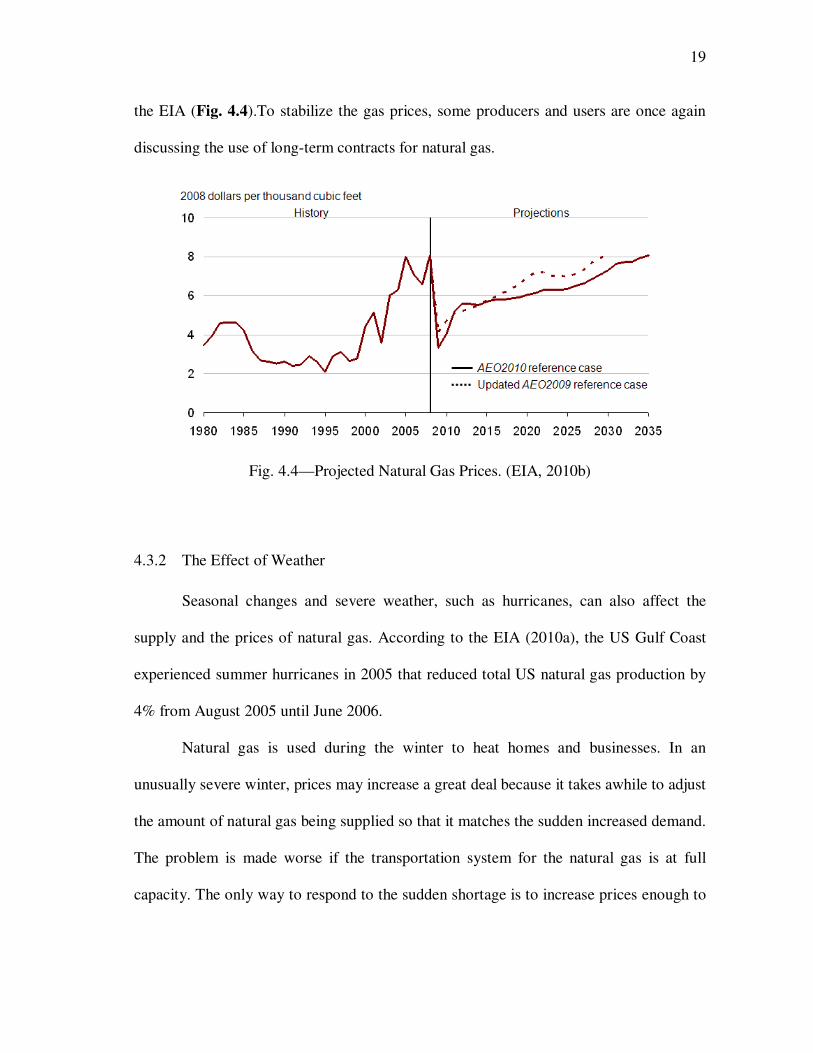
the EIA (Fig. 4.4).To stabilize the gas prices, some producers and users are once again
discussing the use of long-term contracts for natural gas.
Fig. 4.4—Projected Natural Gas Prices. (EIA, 2010b)
4.3.2 The Effect of Weather
Seasonal changes and severe weather, such as hurricanes, can also affect the
supply and the prices of natural gas. According to the EIA (2010a), the US Gulf Coast
experienced summer hurricanes in 2005 that reduced total US natural gas production by
4% from August 2005 until June 2006.
Natural gas is used during the winter to heat homes and businesses. In an
unusually severe winter, prices may increase a great deal because it takes awhile to adjust
the amount of natural gas being supplied so that it matches the sudden increased demand.
The problem is made worse if the transportation system for the natural gas is at full
capacity. The only way to respond to the sudden shortage is to increase prices enough to

20
reduce demand. Sometimes, the weather is so severe that gas wells and pipelines freeze,
which decreases supply when demand is at a high point.
Electric power plants are often fueled by natural gas, but the electricity produced
during the summer months primarily powers air conditioning systems. If the summer is a
hot one, the demand for air conditioning increases and the power plants require more
natural gas in order to produce the necessary electricity. The price of natural gas
increases as a result.
4.3.3 Economic Activity
Natural gas markets are also influenced by economic activity. A strong economy
causes a greater demand for goods and services. As a result, the commercial and
industrial sectors that produce those goods and services increase the demand for natural
gas. In particular, this is true of the industrial sector, which uses natural gas to fuel its
plants and to produce fertilizer and pharmaceuticals.
4.3.4 Underground Storage
The overall supply picture is also influenced by the level of gas held in
underground storage fields. Underground storage fields of natural gas can increase the
ability of companies to meet the suddenly increased needs for natural gas that sometimes
occur, making it easier to maintain stable production rates, pipeline operations, and hub
services. A storage field is an effective way to manage sudden shifts in supply and
demand so that the process is smoother and less reactive. The refill season occurs from

21
April to October, when there is less of a need for natural gas, and the stored gas may then
be used during the heating season.
4.3.5 Oil Prices
For certain industrial consumers and generators of electricity, large-volume gas
consumers can use both natural gas and oil as fuel. They switch between the two based
on which one offers the lower price at the time. In addition, the markets for natural gas
and coal can influence each other when natural gas prices fall or increase significantly. In
some parts of the United States, coal-fired generation of electricity is not competitive if
the cost of natural gas is low enough. Fuel markets do clearly interact with each other.If
oil prices fall, demand shifts from natural gas to oil and natural gas prices go down. If oil
prices rise, consumers may switch back to natural gas from oil, and the natural gas prices
will go up(Fig. 4.5).
Fig. 4.5—Gas Prices Trail Oil Prices (EIA, 2010b)
0
5
10
15
20
25
1990 1995 2000 2005 2010 2015 2020 2025 2030 2035
2008 dollars per million Btu

22
5 INVESTMENT HURDLE: WHAT IS ECONOMICAL?
5.1 Abundant Resources
With significant advances in horizontal drilling technologies, hydraulic
fracturing, and generally higher natural gas prices in the past decade, unconventional gas
reservoirs have become more economic to develop. The EIA estimates that TRR of
natural gas in the US is more than 1,744 trillion cubic feet (Tcf) (EIA, 2007).
Unconventional gas accounts for 60% of the onshore recoverable resource and shale gas
accounts for 28% or more of natural gas TRR in the US (Navigant,
2008).Unconventional gas resources including coalbed methane, tight gas, and gas shale
are abundant in the US. Shale gas are present across much of the lower 48 States (Fig.
5.1).
Fig. 5.1—United States 25 North American Basins (Singh, 2006)

23
Fig. 5.2 shows approximate locations for currently producing or prospective gas
shales. In 2008, the most active shale gas plays were the Barnett, the
Haynesville/Bossier, the Antrim, the Fayetteville, the Marcellus, and the New Albany
(DOE,2009).
Fig. 5.2—United States Shale Gas Basins. (DOE, 2009)
Table 5.1—TRR for United States Shale Gas Basins. (Navigant, 2008)
Barnett Fayetteville Haynesville Marcellus Woodford Antrim New Albany
44 Tcf 41.6Tcf 251Tcf 262Tcf 11.4Tcf 20Tcf 19.2Tcf
To illustrate how rapid the situation can change, one of the most active plays in
the US is now the Eagle Ford Shale in South Texas. The Eagle Ford Shale was not even
mentioned in the DOE (2009) report (Table 5.1).

24
5.2 Investment Hurdle Criteria
There could be several methods to determine what is considered economic. Many
engineers use a PV10 value greater than zero as an indication the well is economic. We
chose to use another definition that relies mainly on Payout and ROR. In this research, a
resource is considered economical if, in a typical well-life of 25years, the wellpays out
its finding and development cost in five years or less and makes at least 20% rate of
return.

25
6 CASE STUDY: THE BARNETT SHALE
6.1 The Barnett Shale: A Hot Play
The Barnett Shale play is located at depths of 6,500–8,500 feet. It is a Mississippian-
age shale with net thickness ranging from 100 to 600 ft. The Total Organic Content
(TOC) is averaged at 4.5%. The total porosity is 4-5%. According to DOE (2009), the
Barnett Shale has an OGIP of 327 Tcf and an estimated TRR of 44 Tcf.
The Barnett Shale play spans 20 to 24 counties in the Fort Worth Basin of north
Texas (Fig. 6.1).The shale’s eastern border is the Ouachita Thrust-fold Belt and the
Muenster Arch; the western border is the Bend Arch. Heading northeast in the play, the
Forestburg limestone splits the Barnett into the upper and lower Barnett. Most
development has focused on the Lower Barnett.
Fig. 6.1—Barnett Shale in the Fort Worth Basin.(DOE,2009)
26
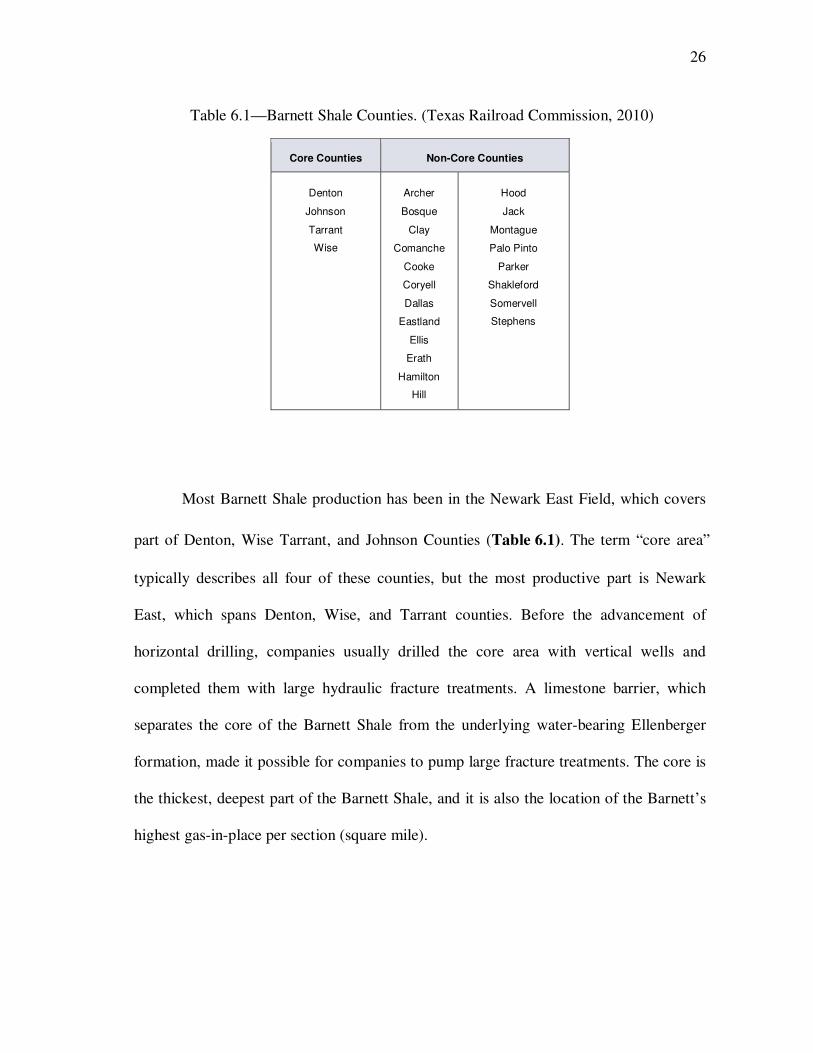
Table 6.1—Barnett Shale Counties. (Texas Railroad Commission, 2010)
Core Counties Non-Core Counties
Denton
Johnson
Tarrant
Wise
Archer
Bosque
Clay
Comanche
Cooke
Coryell
Dallas
Eastland
Ellis
Erath
Hamilton
Hill
Hood
Jack
Montague
Palo Pinto
Parker
Shakleford
Somervell
Stephens
Most Barnett Shale production has been in the Newark East Field, which covers
part of Denton, Wise Tarrant, and Johnson Counties (Table 6.1). The term “core area”
typically describes all four of these counties, but the most productive part is Newark
East, which spans Denton, Wise, and Tarrant counties. Before the advancement of
horizontal drilling, companies usually drilled the core area with vertical wells and
completed them with large hydraulic fracture treatments. A limestone barrier, which
separates the core of the Barnett Shale from the underlying water-bearing Ellenberger
formation, made it possible for companies to pump large fracture treatments. The core is
the thickest, deepest part of the Barnett Shale, and it is also the location of the Barnett’s
highest gas-in-place per section (square mile).

27
The non-core area of the Barnett Shale is located north, south and west of the
core area. According to Hayden (2005), the Viola Limestone separates the core area from
underlying water-bearing formations. In the non-core area where Viola is absent,
however, vertical wells with large hydraulic fracture treatments are at risk of
communicating with the underlying water-bearing Ellenburger formation. To avoid the
problem, companies have effectively used horizontal drilling and multiples of smaller
hydraulic fracture treatments along the horizontal well section. The far west and south
areas of the Fort West basin is the least-developed area. Results from conventional
analysis suggest that a large portion of these areas will produce oil instead of gas
(Hayden, 2005).
Companies that are attempting to develop the non-core area are trying to identify
the west side of the oil-gas window, but without much success yet. In addition to the fact
that they don’t know how far west they can successfully find gas instead of oil, the west
and south shale itself is thinner and shallower. As a result, companies produce lower
amounts of gas-in-place and recovery per section than the Core area. Moreover, the base
of the Barnett does not have a competent fracture barrier, so most operators are using
horizontal wells, which are more expensive, to develop the resource. Since 2006, more
drilling has been taking place on the non-core area.
The rig count in the play has increased as many of the larger players have added
rigs. Currently, production from the Barnett is approximately 1.7Tcf/d (Fig. 6.2). It
accounts for more than 6% of all natural gas produced in the lower 48 States (DOE,
2009).

28
Fig. 6.2—Barnett Shale Annual Total Gas Production. (Texas Railroad Commission,
2010)
Since 1993, more than 13,000 wells have been drilled in the Barnett, far outside
its original core area, due to significant developments in horizontal drilling and light sand
fracturing (Fig. 6.3).The combination of sequenced hydraulic fracture treatments and
horizontal well completions has been crucial in facilitating the expansion of shale gas
development (DOE, 2009).

29
Fig. 6.3—Barnett Shale Well Count from 1993 through 2009. (Texas Railroad
Commission, 2010)
According to the Texas Railroad Commission (2010), 1,162 well permits were
issued through August 2009. In addition, the field produced 809billion cubic feet (Bcf)
of natural gas during the first six months of 2009.
6.2 Barnett Shale Production Profile
To study the economics of producing gas from the Barnett Shale, EUR values
were obtained for approximately 14,000 wells that have been drilled since 1980.The
EUR values were calculated by Unconventional Gas Resources LLC, with a 6% terminal
decline rate. These data were loaded in @Risk® and a log-normal distribution was fitted

30
through the EUR values, which were ranked from lowest to highest. After fitting a
distribution through the EUR values, we ran Monte Carlo simulation runs (with 100,000
random EUR values) to generate a Cumulative Distribution graph. A cumulative
distribution plot shows on the y-axis the percentage of data samples that have a value
lower than the value on the x-axis.
The simulation results provided a probabilistic distribution with a P10 value of
.250 Bcf, a P50 of 1.5 Bcf, and a P90 of 4.0 Bcf. This can be interpreted as follows:
- 90% of the Barnett Shale wells have an EUR of .250 Bcf or more.
- 50% of the Barnett Shale wells have an EUR of 1.5 Bcf
- 10% of the Barnett Shale wells have an EUR of 4.0 Bcf or more.
Based on this distribution, the economic analysis in the next section will be
performed on three wells representing the 10th percentile, 50th percentile, and 90th
percentile, respectively (Table 6.2).
Table 6.2—EUR Values for P10 Well, P50 Well, and P90 Well.
P10 Well P50 Well P90 Well
EUR (Bcf) .250 1.5 4.0
Percentile 10th 50
th 90
th
6.3 Production Forecast Using Hyperbolic Decline Curves
To create the production profile for P10 Well, P50 Well, and P90, hyperbolic
decline curves were used to generate a 40-year production forecast for each well.
Hyperbolic decline curves are concave upward curves when plotted on semi-logarithmic
graph paper and expressed by the following equations:

31
where:
q(t) = production rate at time t, (volume/time)
q(i) = production rate at time t=0, (volume/time)
D(i) = Initial nominal decline rate at t=0, (1/time)
b= hyperbolic exponent
t = time
Gp(t) = Cumulative production for time t.
The b value ranges between 0 and 1, where at b = 0 the hyperbolic decline
becomes exponential decline and at b = 1, the hyperbolic decline becomes harmonic.
However, it is found that in fractured low-permeability formations, the value of exponent
b can be calculated (Mian 2002).Since we only have EUR estimates without production
history to match, we used trial and error to determine q(i), D(i), and b values which yield
the specified EUR values in a 40-year well life. Table 6.3 shows the values used for
generating each production profile. A 10% minimum decline rate was imposed. Fig. 6.4
illustrates the production forecast for each well.
Table 6.3—Input to the Hyperbolic Decline Curve for P10, P50, and P90 Wells.
P10 P50 P90
q(i)(Mcf/d) 700 1600 1500
D(i) 40 10 .5
b 2 2.53 2.52
EUR (Bcf) .250 1.50 4
Min. decline rate 10% 10% 10%

32
Fig. 6.4—40-Year Production Forecast for P10, P50, and P90 Wells.
With the 40-year production forecastfor each well generated, the first 25-year
production profile was captured to economically study each well (Fig. 6.5)
1.0
10.0
100.0
1,000.0
10,000.0
0 5 10 15 20 25 30 35 40 45
Vo
lum
es
(Mcf
/da
y)
Year
Flow Rate vs. Time
P10
P50
P90
33
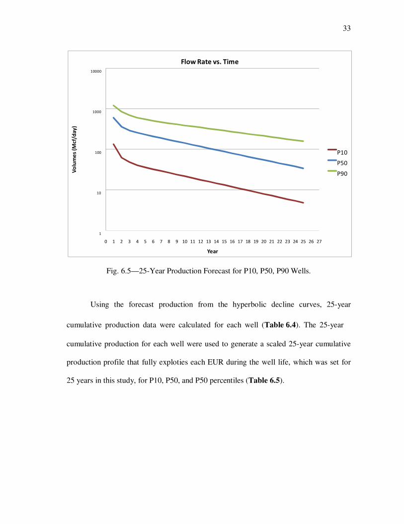
Fig. 6.5—25-Year Production Forecast for P10, P50, P90 Wells.
Using the forecast production from the hyperbolic decline curves, 25-year
cumulative production data were calculated for each well (Table 6.4). The 25-year
cumulative production for each well were used to generate a scaled 25-year cumulative
production profile that fully exploties each EUR during the well life, which was set for
25 years in this study, for P10, P50, and P50 percentiles (Table 6.5).
1
10
100
1000
10000
0 1 2 3 4 5 6 7 8 9 10 11 12 13 14 15 16 17 18 19 20 21 22 23 24 25 26 27
Vo
lum
es
(Mcf
/da
y)
Year
Flow Rate vs. Time
P10
P50
P90

34
Table 6.4—25-Year Production Profile before Scaling.
Years P10 (Mcf) P50 (Mcf) P90 (Mcf)
1 0 0 0
2 51,135 237,688 430,936
3 74,712 376,502 733,030
4 92,837 489,665 981,815
5 108,128 588,735 1,199,066
6 121,605 678,043 1,394,782
7 133,755 758,851 1,574,552
8 144,749 831,970 1,741,888
9 154,697 898,130 1,899,074
10 163,698 957,994 2,047,104
11 171,843 1,012,162 2,186,514
12 179,212 1,061,175 2,317,805
13 185,880 1,105,523 2,441,450
14 191,914 1,145,652 2,557,895
15 197,373 1,181,961 2,667,558
16 202,313 1,214,815 2,770,835
17 206,783 1,244,543 2,868,098
18 210,827 1,271,442 2,959,697
19 214,487 1,295,781 3,045,961
20 217,798 1,317,804 3,127,202
21 220,795 1,337,731 3,203,712
22 223,506 1,355,762 3,275,766
23 225,959 1,372,077 3,343,624
24 228,178 1,386,839 3,407,530
25 230,187 1,400,197 3,467,714
26 232,004 1,412,283 3,524,394

35
Table 6.5—25-Year Production Profile after Scaling to Produce All EUR.
Years P10 (Mcf) P50 (Mcf) P90 (Mcf)
1 0 0 0
2 53,979 245,714 489,090
3 79,313 391,309 831,951
4 98,887 510,104 1,114,308
5 115,456 614,083 1,360,877
6 130,089 707,809 1,583,003
7 143,286 792,728 1,787,033
8 155,228 869,759 1,976,950
9 166,032 939,700 2,155,348
10 175,809 1,003,226 2,323,355
11 184,655 1,060,933 2,481,577
12 192,660 1,113,363 2,630,585
13 199,902 1,161,005 2,770,916
14 206,456 1,204,303 2,903,075
15 212,386 1,243,659 3,027,537
16 217,751 1,279,438 3,144,751
17 222,606 1,311,970 3,255,139
18 226,999 1,341,556 3,359,099
19 230,974 1,368,467 3,457,004
20 234,570 1,392,949 3,549,208
21 237,825 1,415,226 3,636,042
22 240,769 1,435,500 3,717,820
23 243,434 1,453,956 3,794,835
24 245,845 1,470,759 3,867,365
25 248,026 1,486,062 3,935,672
26 250,000 1,500,000 4,000,000
Fig. 6.6 illustrates the cumulative production data throughout the 25-year life for
each well.

36
Fig. 6.6—25-Year Cumulative Production for P10, P50, and P90 Wells.
0.00
250.00
500.00
750.00
1,000.00
1,250.00
1,500.00
1,750.00
2,000.00
2,250.00
2,500.00
2,750.00
3,000.00
3,250.00
3,500.00
3,750.00
4,000.00
4,250.00
0 1 2 3 4 5 6 7 8 9 10 11 12 13 14 15 16 17 18 19 20 21 22 23 24 25 26 27 28
Vo
lum
es
(Msc
f/y
ear
s)
Th
ou
san
ds
Year
Cumulative Production vs. Time
P10
P50
P90
EUR = 4.0 Bcf
EUR = 1.5 Bcf
EUR =.250 Bcf

37
7 ECONOMIC ANALYSIS
7.1 Well-Level Economics: Scenario I
As a starting point, the economic analysis below will be performed using the
following assumptions:
Assumptions for Scenario I
- F&DC of $2 million;
- 0% royalty burden;
- 100% probability of success;
- 0% escalation of gas prices and costs;
- 0% fuel and shrinkage;
- LOE of $1.0/Mcf; and
- 10% annual discount rate.
Fuel shrinkage results from the usage of a percentage of produced gas for
mechanical compression along the pipeline. The well life used for the analysis is 25
years with a 10% annual discount rate. In section 7.2, more realistic assumptions will be
used.
7.1.1 Economics for P10, P50, P90 Wells at Scenario I
With the 25-year production profile for the three wells, representing the 10th, 50th,
and 90thpercentiles, we ran economics on each well, calculating the required gas price

38
that yields an ROR greater than or equal to 20% and pays out the initial investment
(F&DC) in five years or less. We ran several economical scenarios, with F&DC ranging
from $250,000 per well to $400,000, in increments of $250,000 (Table 7.1).
Table 7.1—Gas Prices to Meet Investment Hurdle at Different F&D Costs at Scenario I
EUR (Bcf) 0.25 EUR (Bcf) 1.5 EUR (Bcf) 4.00
P10 P50 P90
F&DC Gas Price per Mcf
F&DC Gas Price per Mcf
F&DC Gas Price per Mcf
$250,000 $3.40 $250,000 $1.50 $250,000 $1.20
$500,000 $5.70 $500,000 $1.90 $500,000 $1.40
$750,000 $8.10 $750,000 $2.30 $750,000 $1.60
$1,000,000 $10.40 $1,000,000 $2.80 $1,000,000 $1.80
$1,250,000 $12.80 $1,250,000 $3.20 $1,250,000 $2.00
$1,500,000 $15.10 $1,500,000 $3.60 $1,500,000 $2.20
$1,750,000 $17.50 $1,750,000 $4.10 $1,750,000 $2.40
$2,000,000 $19.80 $2,000,000 $4.50 $2,000,000 $2.60
$2,250,000 $22.20 $2,250,000 $4.90 $2,250,000 $2.70
$2,500,000 $24.50 $2,500,000 $5.40 $2,500,000 $2.90
$2,750,000 $26.90 $2,750,000 $5.80 $2,750,000 $3.10
$3,000,000 $29.20 $3,000,000 $6.20 $3,000,000 $3.30
$3,250,000 $31.60 $3,250,000 $6.70 $3,250,000 $3.50
$3,500,000 $33.90 $3,500,000 $7.10 $3,500,000 $3.70
$3,750,000 $36.30 $3,750,000 $7.50 $3,750,000 $3.90
$4,000,000 $38.60 $4,000,000 $8.00 $4,000,000 $4.10
As the EUR increases, the required gas price to meet our investment-hurdle
decreases (Fig. 7.1). For example, a Barnett Shale well with an EUR of 1.5 Bcf that costs
$2 million to be drilled and completed will require agas price of $4.5/Mcf before it can
be considered economical, while a 4.0-Bcf well with the same F&DC will require a gas
price of $2.6/Mcf before it will be worth the investment.

39
Fig. 7.1—Gas Prices Required to Meet Investment Hurdle at Different F&D
Costs(Scenario I).
Tables 7.2, 7.3 and 7.4 show detailed economic analysis, converting the 25-year
stream of gas production to a stream of cash flow for the P10, P50, and P90 wells at
Scenario I.
$0.00 $10.00 $20.00 $30.00 $40.00 $50.00
$250,000
$500,000
$750,000
$1,000,000
$1,250,000
$1,500,000
$1,750,000
$2,000,000
$2,250,000
$2,500,000
$2,750,000
$3,000,000
$3,250,000
$3,500,000
$3,750,000
$4,000,000
Gas Price $/Mcf
F&D
C
P90
P50
P10

40
Table 7.2—Detailed Economic Analysis for a P10 Well with an F&DC of $2 Million (Scenario I)
Payout: 4.39 Years
Payout Year: 4
Economic Limit Year: 26
$2,430,000 $2,430,000 $2,430,000 $2,430,000 225,000 $684,721 $684,721
225,000
Final Final Cum
Net Cum Net Net Cum Net Risked Disc. Disc.
Cash Flow Profit Cash Flow Profit Gross Discount Profit Profit
Time ($) ($) ($) ($) Prod Factor ($) ($)
(Years) $0 $0 $0 $0 (Mscf) (%/yr) $0 $0
1 ($1,800,000) ($1,800,000) ($1,800,000) ($1,800,000) 0 1 ($1,800,000) ($1,800,000)
2 $932,316 ($867,684) $932,316 ($867,684) 49,591 0.909090909 $847,560 ($952,440)
3 $429,865 ($437,819) $429,865 ($437,819) 22,865 0.826446281 $355,260 ($597,180)
4 $330,459 ($107,360) $330,459 ($107,360) 17,578 0.751314801 $248,279 ($348,901)
5 $278,797 $171,437 $278,797 $171,437 14,830 0.683013455 $190,422 ($158,478)
6 $245,725 $417,162 $245,725 $417,162 13,070 0.620921323 $152,576 ($5,903)
7 $221,527 $638,690 $221,527 $638,690 11,783 0.56447393 $125,046 $119,144
8 $200,446 $839,136 $200,446 $839,136 10,662 0.513158118 $102,861 $222,004
9 $181,371 $1,020,507 $181,371 $1,020,507 9,647 0.46650738 $84,611 $306,615
10 $164,111 $1,184,618 $164,111 $1,184,618 8,729 0.424097618 $69,599 $376,215
11 $148,494 $1,333,113 $148,494 $1,333,113 7,899 0.385543289 $57,251 $433,466
12 $134,363 $1,467,476 $134,363 $1,467,476 7,147 0.350493899 $47,093 $480,559
13 $121,577 $1,589,053 $121,577 $1,589,053 6,467 0.318630818 $38,738 $519,297
14 $110,007 $1,699,060 $110,007 $1,699,060 5,851 0.28966438 $31,865 $551,162
15 $99,539 $1,798,598 $99,539 $1,798,598 5,295 0.263331254 $26,212 $577,374
16 $90,066 $1,888,665 $90,066 $1,888,665 4,791 0.239392049 $21,561 $598,935
17 $81,495 $1,970,160 $81,495 $1,970,160 4,335 0.217629136 $17,736 $616,671
18 $73,740 $2,043,900 $73,740 $2,043,900 3,922 0.197844669 $14,589 $631,260
19 $66,723 $2,110,623 $66,723 $2,110,623 3,549 0.17985879 $12,001 $643,261
20 $60,373 $2,170,996 $60,373 $2,170,996 3,211 0.163507991 $9,872 $653,132
21 $54,628 $2,225,624 $54,628 $2,225,624 2,906 0.148643628 $8,120 $661,252
22 $49,429 $2,275,053 $49,429 $2,275,053 2,629 0.135130571 $6,679 $667,932
23 $44,726 $2,319,779 $44,726 $2,319,779 2,379 0.122845974 $5,494 $673,426
24 $40,469 $2,360,248 $40,469 $2,360,248 2,153 0.111678158 $4,520 $677,945 25 $36,618 $2,396,866 $36,618 $2,396,866 1,948 0.101525598 $3,718 $681,663
26 $33,134 $2,430,000 $33,134 $2,430,000 1,762 0.092295998 $3,058 $684,721
41
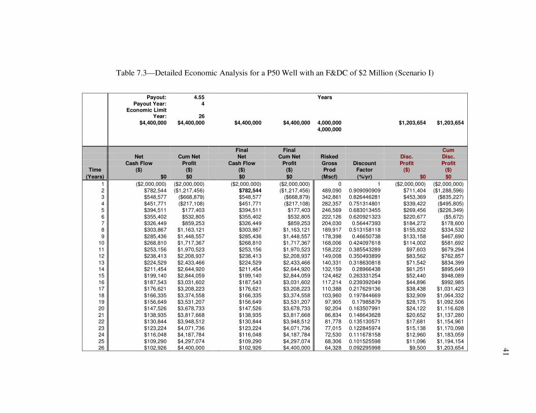
Table 7.3—Detailed Economic Analysis for a P50 Well with an F&DC of $2 Million (Scenario I)
Payout: 4.55 Years Payout Year: 4
Economic Limit
Year: 26 $4,400,000 $4,400,000 $4,400,000 $4,400,000 4,000,000 $1,203,654 $1,203,654
4,000,000
Final Final Cum Net Cum Net Net Cum Net Risked Disc. Disc.
Cash Flow Profit Cash Flow Profit Gross Discount Profit Profit Time ($) ($) ($) ($) Prod Factor ($) ($)
(Years) $0 $0 $0 $0 (Mscf) (%/yr) $0 $0
1 ($2,000,000) ($2,000,000) ($2,000,000) ($2,000,000) 0 1 ($2,000,000) ($2,000,000) 2 $782,544 ($1,217,456) $782,544 ($1,217,456) 489,090 0.909090909 $711,404 ($1,288,596) 3 $548,577 ($668,879) $548,577 ($668,879) 342,861 0.826446281 $453,369 ($835,227)
4 $451,771 ($217,108) $451,771 ($217,108) 282,357 0.751314801 $339,422 ($495,805) 5 $394,511 $177,403 $394,511 $177,403 246,569 0.683013455 $269,456 ($226,349)
6 $355,402 $532,805 $355,402 $532,805 222,126 0.620921323 $220,677 ($5,672) 7 $326,449 $859,253 $326,449 $859,253 204,030 0.56447393 $184,272 $178,600 8 $303,867 $1,163,121 $303,867 $1,163,121 189,917 0.513158118 $155,932 $334,532
9 $285,436 $1,448,557 $285,436 $1,448,557 178,398 0.46650738 $133,158 $467,690 10 $268,810 $1,717,367 $268,810 $1,717,367 168,006 0.424097618 $114,002 $581,692
11 $253,156 $1,970,523 $253,156 $1,970,523 158,222 0.385543289 $97,603 $679,294 12 $238,413 $2,208,937 $238,413 $2,208,937 149,008 0.350493899 $83,562 $762,857
13 $224,529 $2,433,466 $224,529 $2,433,466 140,331 0.318630818 $71,542 $834,399 14 $211,454 $2,644,920 $211,454 $2,644,920 132,159 0.28966438 $61,251 $895,649 15 $199,140 $2,844,059 $199,140 $2,844,059 124,462 0.263331254 $52,440 $948,089
16 $187,543 $3,031,602 $187,543 $3,031,602 117,214 0.239392049 $44,896 $992,985 17 $176,621 $3,208,223 $176,621 $3,208,223 110,388 0.217629136 $38,438 $1,031,423
18 $166,335 $3,374,558 $166,335 $3,374,558 103,960 0.197844669 $32,909 $1,064,332 19 $156,649 $3,531,207 $156,649 $3,531,207 97,905 0.17985879 $28,175 $1,092,506 20 $147,526 $3,678,733 $147,526 $3,678,733 92,204 0.163507991 $24,122 $1,116,628
21 $138,935 $3,817,668 $138,935 $3,817,668 86,834 0.148643628 $20,652 $1,137,280 22 $130,844 $3,948,512 $130,844 $3,948,512 81,778 0.135130571 $17,681 $1,154,961
23 $123,224 $4,071,736 $123,224 $4,071,736 77,015 0.122845974 $15,138 $1,170,098 24 $116,048 $4,187,784 $116,048 $4,187,784 72,530 0.111678158 $12,960 $1,183,059
25 $109,290 $4,297,074 $109,290 $4,297,074 68,306 0.101525598 $11,096 $1,194,154 26 $102,926 $4,400,000 $102,926 $4,400,000 64,328 0.092295998 $9,500 $1,203,654

42
Table 7.4—Detailed Economic Analysis for a P90 Well with an F&DC of $2 Million (Scenario I)
Payout: 4.59 Years
Payout Year: 4
Economic Limit
Year: 26 $3,250,000 $3,250,000 $3,250,000 $3,250,000 1,500,000 $909,518 $909,518
1,500,000
Final Final Cum
Net Cum Net Net Cum Net Risked Disc. Disc. Cash Flow Profit Cash Flow Profit Gross Discount Profit Profit
Time ($) ($) ($) ($) Prod Factor ($) ($)
(Years) $0 $0 $0 $0 (Mscf) (%/yr) $0 $0
1 ($2,000,000) ($2,000,000) ($2,000,000) ($2,000,000) 0 1 ($2,000,000) ($2,000,000)
2 $859,999 ($1,140,001) $859,999 ($1,140,001) 245,714 0.909090909 $781,817 ($1,218,183)
3 $509,581 ($630,420) $509,581 ($630,420) 145,595 0.826446281 $421,141 ($797,041) 4 $415,785 ($214,635) $415,785 ($214,635) 118,796 0.751314801 $312,385 ($484,656)
5 $363,925 $149,290 $363,925 $149,290 103,979 0.683013455 $248,566 ($236,090)
6 $328,042 $477,332 $328,042 $477,332 93,726 0.620921323 $203,688 ($32,402) 7 $297,214 $774,546 $297,214 $774,546 84,918 0.56447393 $167,770 $135,368
8 $269,610 $1,044,156 $269,610 $1,044,156 77,031 0.513158118 $138,352 $273,720 9 $244,792 $1,288,949 $244,792 $1,288,949 69,941 0.46650738 $114,197 $387,918
10 $222,341 $1,511,289 $222,341 $1,511,289 63,526 0.424097618 $94,294 $482,212
11 $201,977 $1,713,266 $201,977 $1,713,266 57,708 0.385543289 $77,871 $560,083 12 $183,504 $1,896,771 $183,504 $1,896,771 52,430 0.350493899 $64,317 $624,400
13 $166,746 $2,063,517 $166,746 $2,063,517 47,642 0.318630818 $53,131 $677,530
14 $151,542 $2,215,059 $151,542 $2,215,059 43,298 0.28966438 $43,896 $721,427 15 $137,746 $2,352,805 $137,746 $2,352,805 39,356 0.263331254 $36,273 $757,700
16 $125,226 $2,478,032 $125,226 $2,478,032 35,779 0.239392049 $29,978 $787,678 17 $113,864 $2,591,896 $113,864 $2,591,896 32,533 0.217629136 $24,780 $812,458
18 $103,550 $2,695,446 $103,550 $2,695,446 29,586 0.197844669 $20,487 $832,945
19 $94,188 $2,789,634 $94,188 $2,789,634 26,911 0.17985879 $16,941 $849,885 20 $85,688 $2,875,321 $85,688 $2,875,321 24,482 0.163507991 $14,011 $863,896
21 $77,970 $2,953,291 $77,970 $2,953,291 22,277 0.148643628 $11,590 $875,486
22 $70,960 $3,024,251 $70,960 $3,024,251 20,274 0.135130571 $9,589 $885,075 23 $64,594 $3,088,846 $64,594 $3,088,846 18,456 0.122845974 $7,935 $893,010
24 $58,812 $3,147,658 $58,812 $3,147,658 16,803 0.111678158 $6,568 $899,578 25 $53,558 $3,201,216 $53,558 $3,201,216 15,302 0.101525598 $5,438 $905,015
26 $48,784 $3,250,000 $48,784 $3,250,000 13,938 0.092295998 $4,503 $909,518

43
7.1.2 Economics for P* Well at Scenario I
Based on the P10, P50, and P90 EUR values, a weighted EUR for P* Well was
calculated as follows:
P* Weighted EUR = P10 EUR * 16% + P50 EUR * 68% + P90 EUR * 16 %
P* Weighted EUR = (0.250 * 0.16) + (1.5 * 0.68) + (4.0 * 0.16) = 1.7 Bcf
The weighting factors have been selected so the values are approximately one
standard deviation from the mean (Fig. 7.2).
Fig. 7.2—Confidence Intervals for a Normal Distribution Curve.
Table 7.5 and Fig. 7.3 compare the required gas prices to meet the investment
hurdle criteria for the P10, P50, P90, and P* Wells at different F&DC costs.

44
Table 7.5—Gas Prices to Meet Investment Hurdle at Different F&DCs for a P10, P50, P90, and P* Well. (Scenario I)
EUR (Bcf) 0.25 EUR
(Bscf) 1.5 EUR (Bcf) 4.00 EUR (Bcf) 1.7
P10 P50 P90 P*
F&DC Gas Price per Mscf
F&DC Gas Price per Mcf
F&DC Gas Price per Mcf
F&DC Gas Price per Mcf
$250,000 $3.40 $250,000 $1.50 $250,000 $1.20 $250,000 $1.50
$500,000 $5.70 $500,000 $1.90 $500,000 $1.40 $500,000 $1.90
$750,000 $8.10 $750,000 $2.30 $750,000 $1.60 $750,000 $2.30
$1,000,000 $10.40 $1,000,000 $2.80 $1,000,000 $1.80 $1,000,000 $2.70
$1,250,000 $12.80 $1,250,000 $3.20 $1,250,000 $2.00 $1,250,000 $3.10
$1,500,000 $15.10 $1,500,000 $3.60 $1,500,000 $2.20 $1,500,000 $3.50
$1,750,000 $17.50 $1,750,000 $4.10 $1,750,000 $2.40 $1,750,000 $3.90
$2,000,000 $19.80 $2,000,000 $4.50 $2,000,000 $2.60 $2,000,000 $4.30
$2,250,000 $22.20 $2,250,000 $4.90 $2,250,000 $2.70 $2,250,000 $4.70
$2,500,000 $24.50 $2,500,000 $5.40 $2,500,000 $2.90 $2,500,000 $5.10
$2,750,000 $26.90 $2,750,000 $5.80 $2,750,000 $3.10 $2,750,000 $5.50
$3,000,000 $29.20 $3,000,000 $6.20 $3,000,000 $3.30 $3,000,000 $5.90
$3,250,000 $31.60 $3,250,000 $6.70 $3,250,000 $3.50 $3,250,000 $6.30
$3,500,000 $33.90 $3,500,000 $7.10 $3,500,000 $3.70 $3,500,000 $6.70
$3,750,000 $36.30 $3,750,000 $7.50 $3,750,000 $3.90 $3,750,000 $7.10
$4,000,000 $38.60 $4,000,000 $8.00 $4,000,000 $4.10 $4,000,000 $7.50

45
Fig. 7.3—Gas Prices to Meet Investment Hurdle at Different F&DCs a P10, P50, P90,
and P* Well(Scenario I).
Table 7.6 shows detailed economic analysis, converting the 25-year stream of
gas production to a stream of cash flows for the P* well at Scenario I.
$0.00 $10.00 $20.00 $30.00 $40.00 $50.00
$250,000
$500,000
$750,000
$1,000,000
$1,250,000
$1,500,000
$1,750,000
$2,000,000
$2,250,000
$2,500,000
$2,750,000
$3,000,000
$3,250,000
$3,500,000
$3,750,000
$4,000,000
Gas Price $/Mcf
F&D
C
P*
P90
P50
P10

46
Table 7.6—Detailed Economic Analysis for a P*Well with an F&DC of $2 Million (Scenario I)
Payout: 4.58 Years Payout Year: 4
Economic Limit
Year: 26 $3,610,000 $3,610,000 $3,610,000 $3,610,000 1,700,000 $999,848 $999,848 1,700,000
Final Final Cum Net Cum Net Net Cum Net Risked Disc. Disc. Cash Flow Profit Cash Flow Profit Gross Discount Profit Profit
Time ($) ($) ($) ($) Prod Factor ($) ($)
(Years) $0 $0 $0 $0 (Mscf) (%/yr) $0 $0
1 ($2,000,000) ($2,000,000) ($2,000,000) ($2,000,000) 0 1 ($2,000,000) ($2,000,000) 2 $838,123 ($1,161,877) $838,123 ($1,161,877) 253,977 0.909090909 $761,930 ($1,238,070) 3 $521,121 ($640,756) $521,121 ($640,756) 157,915 0.826446281 $430,679 ($807,392) 4 $425,997 ($214,759) $425,997 ($214,759) 129,090 0.751314801 $320,058 ($487,334) 5 $372,265 $157,505 $372,265 $157,505 112,807 0.683013455 $254,262 ($233,072) 6 $335,331 $492,837 $335,331 $492,837 101,615 0.620921323 $208,214 ($24,858) 7 $305,253 $798,089 $305,253 $798,089 92,501 0.56447393 $172,307 $147,450 8 $279,440 $1,077,529 $279,440 $1,077,529 84,679 0.513158118 $143,397 $290,846 9 $256,846 $1,334,375 $256,846 $1,334,375 77,832 0.46650738 $119,820 $410,667
10 $236,422 $1,570,797 $236,422 $1,570,797 71,643 0.424097618 $100,266 $510,933 11 $217,708 $1,788,505 $217,708 $1,788,505 65,972 0.385543289 $83,936 $594,869 12 $200,555 $1,989,060 $200,555 $1,989,060 60,774 0.350493899 $70,293 $665,162 13 $184,827 $2,173,887 $184,827 $2,173,887 56,008 0.318630818 $58,892 $724,054 14 $170,400 $2,344,287 $170,400 $2,344,287 51,636 0.28966438 $49,359 $773,412 15 $157,162 $2,501,449 $157,162 $2,501,449 47,625 0.263331254 $41,386 $814,798 16 $145,010 $2,646,459 $145,010 $2,646,459 43,942 0.239392049 $34,714 $849,512 17 $133,851 $2,780,310 $133,851 $2,780,310 40,561 0.217629136 $29,130 $878,642 18 $123,601 $2,903,911 $123,601 $2,903,911 37,455 0.197844669 $24,454 $903,096 19 $114,181 $3,018,092 $114,181 $3,018,092 34,600 0.17985879 $20,536 $923,632 20 $105,521 $3,123,613 $105,521 $3,123,613 31,976 0.163507991 $17,253 $940,886 21 $97,556 $3,221,169 $97,556 $3,221,169 29,563 0.148643628 $14,501 $955,387 22 $90,229 $3,311,398 $90,229 $3,311,398 27,342 0.135130571 $12,193 $967,580 23 $83,485 $3,394,883 $83,485 $3,394,883 25,299 0.122845974 $10,256 $977,835 24 $77,276 $3,472,159 $77,276 $3,472,159 23,417 0.111678158 $8,630 $986,465 25 $71,556 $3,543,715 $71,556 $3,543,715 21,684 0.101525598 $7,265 $993,730
26 $66,285 $3,610,000 $66,285 $3,610,000 20,086 0.092295998 $6,118 $999,848

47
Using the assumptions detailed at the beginning of the section, Table 7.7
compares the required gas prices to meet the investment hurdle criteria for P10 Well, P50
Well, P90 Well, and P*Well, and the resulting ROR and Payout.
Table 7.7—ROR and Payout Periods for P10, P50, P90, and P* with a $2 Million
F&DC (Scenario I)
P10 Well P50 Well P90 Well P* Well
EUR (Bcf) .250 1.5 Bcf 4.0 Bcf 1.7 Bcf
Gas Price ($/Mcf) 21.0 4.70 2.70 4.50
Payout Period (Years) 4.4 4.6 4.6 4.6
ROR (%) 20 20 22 21
7.2 Well-Level Economics: Scenario II
The economic analysis in this section will be performed at the following
assumptions:
Assumptions for Scenario II
- F&DC of $2 million;
- 25% royalty burden;
- 90% probability of success;
- 0% escalation of gas prices and costs;
- 6% fuel and shrinkage;
- LOE of $1.0/Mcf; and
- 10% annual discount rate.

48
The well life used for the analysis is 25 years with a 10% annual discount rate.
Note that the EURs are lower than the values in
. This occurs because of the assumption that the probability of success is 90%. In
addition, the 25% royalty burden also affects the economic analysis as follows:
EUR at 90% Probability of Success = EUR * 0.9
Net Production = Gross Production * (1 – Royalty Burden)
7.2.1 Economics for P10, P50, P90, and P* Wells at Scenario II
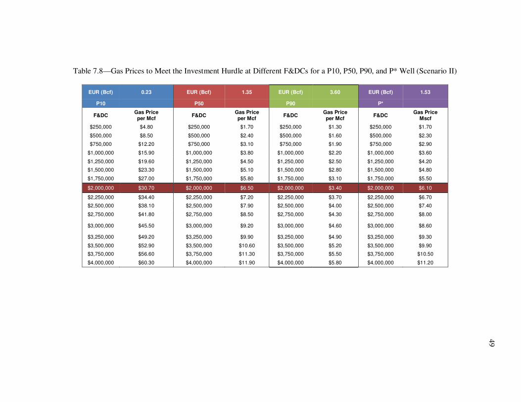
Table 7.8 and Fig. 7.4 compare the required gas prices to meet the investment
hurdle criteria for the P10, P50, P90, and P* Wells at different F&D costs (Scenario II).
Table 7.9, 7.10, 7.11, and 7.12 show detailed economic analysis, converting the 25-year
stream of gas production to a stream of cash flows for the P10, P50, P90, and P* wells
(Scenario II).
49
Table 7.8—Gas Prices to Meet the Investment Hurdle at Different F&DCs for a P10, P50, P90, and P* Well (Scenario II)
EUR (Bcf) 0.23 EUR (Bcf) 1.35 EUR (Bcf) 3.60 EUR (Bcf) 1.53
P10 P50 P90 P*
F&DC Gas Price per Mcf
F&DC Gas Price per Mcf
F&DC Gas Price per Mcf
F&DC Gas Price
Mscf
$250,000 $4.80 $250,000 $1.70 $250,000 $1.30 $250,000 $1.70
$500,000 $8.50 $500,000 $2.40 $500,000 $1.60 $500,000 $2.30
$750,000 $12.20 $750,000 $3.10 $750,000 $1.90 $750,000 $2.90
$1,000,000 $15.90 $1,000,000 $3.80 $1,000,000 $2.20 $1,000,000 $3.60
$1,250,000 $19.60 $1,250,000 $4.50 $1,250,000 $2.50 $1,250,000 $4.20
$1,500,000 $23.30 $1,500,000 $5.10 $1,500,000 $2.80 $1,500,000 $4.80
$1,750,000 $27.00 $1,750,000 $5.80 $1,750,000 $3.10 $1,750,000 $5.50
$2,000,000 $30.70 $2,000,000 $6.50 $2,000,000 $3.40 $2,000,000 $6.10
$2,250,000 $34.40 $2,250,000 $7.20 $2,250,000 $3.70 $2,250,000 $6.70
$2,500,000 $38.10 $2,500,000 $7.90 $2,500,000 $4.00 $2,500,000 $7.40
$2,750,000 $41.80 $2,750,000 $8.50 $2,750,000 $4.30 $2,750,000 $8.00
$3,000,000 $45.50 $3,000,000 $9.20 $3,000,000 $4.60 $3,000,000 $8.60
$3,250,000 $49.20 $3,250,000 $9.90 $3,250,000 $4.90 $3,250,000 $9.30
$3,500,000 $52.90 $3,500,000 $10.60 $3,500,000 $5.20 $3,500,000 $9.90
$3,750,000 $56.60 $3,750,000 $11.30 $3,750,000 $5.50 $3,750,000 $10.50
$4,000,000 $60.30 $4,000,000 $11.90 $4,000,000 $5.80 $4,000,000 $11.20

50
Fig. 7.4—Gas Prices to Meet the Investment Hurdle at Different F&D Costs a P10, P50,
P90, and P* Well (Scenario II).
$0.00 $10.00 $20.00 $30.00 $40.00 $50.00 $60.00 $70.00
$250,000
$500,000
$750,000
$1,000,000
$1,250,000
$1,500,000
$1,750,000
$2,000,000
$2,250,000
$2,500,000
$2,750,000
$3,000,000
$3,250,000
$3,500,000
$3,750,000
$4,000,000
Gas Price $/Mcf
F&D
C
P*
P90
P50
P10

51
Table 7.9—Detailed Economic Analysis for a P10 Well with an F&DC of $2 Million. (Scenario II)
Payout: 4.37 Years
Payout Year: 4
Economic Limit
Year: 26
$2,440,046 $2,440,046 $2,440,046 $2,440,046 202,500 $690,622 $690,622
202,500
Final Final Cum
Net Cum Net Net Cum Net Risked Disc. Disc.
Cash Flow Profit Cash Flow Profit Gross Discount Profit Profit
Time ($) ($) ($) ($) Prod Factor ($) ($)
(Years) $0 $0 $0 $0 (Mscf) (%/yr) $0 $0
1 ($1,800,000) ($1,800,000) ($1,800,000) ($1,800,000) 0 1 ($1,800,000) ($1,800,000)
2 $934,530 ($865,470) $934,530 ($865,470) 44,632 0.909090909 $849,573 ($950,427)
3 $430,886 ($434,584) $430,886 ($434,584) 20,579 0.826446281 $356,104 ($594,323)
4 $331,244 ($103,340) $331,244 ($103,340) 15,820 0.751314801 $248,868 ($345,454)
5 $279,459 $176,120 $279,459 $176,120 13,347 0.683013455 $190,875 ($154,580)
6 $246,309 $422,428 $246,309 $422,428 11,763 0.620921323 $152,938 ($1,642)
7 $222,053 $644,482 $222,053 $644,482 10,605 0.56447393 $125,343 $123,702
8 $200,922 $845,404 $200,922 $845,404 9,596 0.513158118 $103,105 $226,807
9 $181,802 $1,027,206 $181,802 $1,027,206 8,683 0.46650738 $84,812 $311,619
10 $164,501 $1,191,707 $164,501 $1,191,707 7,856 0.424097618 $69,765 $381,383
11 $148,847 $1,340,554 $148,847 $1,340,554 7,109 0.385543289 $57,387 $438,770
12 $134,682 $1,475,236 $134,682 $1,475,236 6,432 0.350493899 $47,205 $485,975
13 $121,865 $1,597,102 $121,865 $1,597,102 5,820 0.318630818 $38,830 $524,805
14 $110,268 $1,707,370 $110,268 $1,707,370 5,266 0.28966438 $31,941 $556,746
15 $99,775 $1,807,145 $99,775 $1,807,145 4,765 0.263331254 $26,274 $583,020
16 $90,280 $1,897,425 $90,280 $1,897,425 4,312 0.239392049 $21,612 $604,632
17 $81,689 $1,979,114 $81,689 $1,979,114 3,901 0.217629136 $17,778 $622,410
18 $73,915 $2,053,029 $73,915 $2,053,029 3,530 0.197844669 $14,624 $637,034
19 $66,881 $2,119,910 $66,881 $2,119,910 3,194 0.17985879 $12,029 $649,063
20 $60,517 $2,180,427 $60,517 $2,180,427 2,890 0.163507991 $9,895 $658,958
21 $54,758 $2,235,185 $54,758 $2,235,185 2,615 0.148643628 $8,139 $667,098
22 $49,547 $2,284,732 $49,547 $2,284,732 2,366 0.135130571 $6,695 $673,793
23 $44,832 $2,329,563 $44,832 $2,329,563 2,141 0.122845974 $5,507 $679,300
24 $40,565 $2,370,129 $40,565 $2,370,129 1,937 0.111678158 $4,530 $683,831
25 $36,705 $2,406,834 $36,705 $2,406,834 1,753 0.101525598 $3,727 $687,557
26 $33,212 $2,440,046 $33,212 $2,440,046 1,586 0.092295998 $3,065 $690,622

52
Table 7.10—Detailed Economic Analysis for a P50 Well with an F&DC of $2 Million. (Scenario II)
Payout: 4.61 Years
Payout Year: 4
Economic Limit Year: 26
$3,234,625 $3,234,625 $3,234,625 $3,234,625 1,350,000 $900,997 $900,997
1,350,000
Final Final Cum Net Cum Net Net Cum Net Risked Disc. Disc. Cash Flow Profit Cash Flow Profit Gross Discount Profit Profit
Time ($) ($) ($) ($) Prod Factor ($) ($)
(Years) $0 $0 $0 $0 (Mscf) (%/yr) $0 $0
1 ($2,000,000) ($2,000,000) ($2,000,000) ($2,000,000) 0 1 ($2,000,000) ($2,000,000) 2 $857,481 ($1,142,519) $857,481 ($1,142,519) 221,143 0.909090909 $779,528 ($1,220,472) 3 $508,089 ($634,431) $508,089 ($634,431) 131,035 0.826446281 $419,908 ($800,564) 4 $414,567 ($219,864) $414,567 ($219,864) 106,916 0.751314801 $311,470 ($489,094) 5 $362,859 $142,996 $362,859 $142,996 93,581 0.683013455 $247,838 ($241,256) 6 $327,081 $470,077 $327,081 $470,077 84,354 0.620921323 $203,092 ($38,164) 7 $296,344 $766,421 $296,344 $766,421 76,427 0.56447393 $167,278 $129,114 8 $268,820 $1,035,241 $268,820 $1,035,241 69,328 0.513158118 $137,947 $267,061 9 $244,076 $1,279,317 $244,076 $1,279,317 62,947 0.46650738 $113,863 $380,925 10 $221,690 $1,501,006 $221,690 $1,501,006 57,173 0.424097618 $94,018 $474,943 11 $201,385 $1,702,392 $201,385 $1,702,392 51,937 0.385543289 $77,643 $552,585 12 $182,967 $1,885,359 $182,967 $1,885,359 47,187 0.350493899 $64,129 $616,714 13 $166,258 $2,051,617 $166,258 $2,051,617 42,878 0.318630818 $52,975 $669,689 14 $151,098 $2,202,715 $151,098 $2,202,715 38,968 0.28966438 $43,768 $713,457 15 $137,343 $2,340,058 $137,343 $2,340,058 35,420 0.263331254 $36,167 $749,624 16 $124,860 $2,464,917 $124,860 $2,464,917 32,201 0.239392049 $29,890 $779,514 17 $113,530 $2,578,448 $113,530 $2,578,448 29,279 0.217629136 $24,708 $804,221 18 $103,247 $2,681,695 $103,247 $2,681,695 26,627 0.197844669 $20,427 $824,648 19 $93,912 $2,775,607 $93,912 $2,775,607 24,220 0.17985879 $16,891 $841,539 20 $85,437 $2,861,044 $85,437 $2,861,044 22,034 0.163507991 $13,970 $855,509 21 $77,741 $2,938,785 $77,741 $2,938,785 20,049 0.148643628 $11,556 $867,065 22 $70,753 $3,009,538 $70,753 $3,009,538 18,247 0.135130571 $9,561 $876,625 23 $64,405 $3,073,943 $64,405 $3,073,943 16,610 0.122845974 $7,912 $884,537 24 $58,639 $3,132,582 $58,639 $3,132,582 15,123 0.111678158 $6,549 $891,086 25 $53,401 $3,185,984 $53,401 $3,185,984 13,772 0.101525598 $5,422 $896,508 26 $48,641 $3,234,625 $48,641 $3,234,625 12,545 0.092295998 $4,489 $900,997

53
Table 7.11—Detailed Economic Analysis for a P90 Well with an F&DC of $2 Million.(Scenario II)
Payout: 4.81 Years Payout Year: 4
Economic Limit Year:
26
$4,091,200 $4,091,200 $4,091,200 $4,091,200 3,600,000 $1,049,078 $1,049,078 3,600,000
Final Final Cum Net Cum Net Net Cum Net Risked Disc. Disc.
Cash Flow Profit Cash Flow Profit Gross Discount Profit Profit Time ($) ($) ($) ($) Prod Factor ($) ($)
(Years) $0 $0 $0 $0 (Mscf) (%/yr) $0 $0
1 ($2,000,000) ($2,000,000) ($2,000,000) ($2,000,000) 0 1 ($2,000,000) ($2,000,000)
2 $744,786 ($1,255,214) $744,786 ($1,255,214) 440,181 0.909090909 $677,078 ($1,322,922) 3 $522,108 ($733,106) $522,108 ($733,106) 308,575 0.826446281 $431,494 ($891,427)
4 $429,973 ($303,132) $429,973 ($303,132) 254,121 0.751314801 $323,045 ($568,382) 5 $375,476 $72,343 $375,476 $72,343 221,912 0.683013455 $256,455 ($311,927)
6 $338,254 $410,597 $338,254 $410,597 199,914 0.620921323 $210,029 ($101,898)
7 $310,697 $721,294 $310,697 $721,294 183,627 0.56447393 $175,381 $73,482 8 $289,206 $1,010,500 $289,206 $1,010,500 170,925 0.513158118 $148,408 $221,891
9 $271,664 $1,282,164 $271,664 $1,282,164 160,558 0.46650738 $126,733 $348,624
10 $255,840 $1,538,004 $255,840 $1,538,004 151,206 0.424097618 $108,501 $457,125 11 $240,941 $1,778,946 $240,941 $1,778,946 142,400 0.385543289 $92,893 $550,019
12 $226,910 $2,005,856 $226,910 $2,005,856 134,107 0.350493899 $79,531 $629,549 13 $213,696 $2,219,551 $213,696 $2,219,551 126,298 0.318630818 $68,090 $697,639
14 $201,251 $2,420,802 $201,251 $2,420,802 118,943 0.28966438 $58,295 $755,934
15 $189,531 $2,610,333 $189,531 $2,610,333 112,016 0.263331254 $49,909 $805,844 16 $178,494 $2,788,827 $178,494 $2,788,827 105,493 0.239392049 $42,730 $848,574
17 $168,099 $2,956,926 $168,099 $2,956,926 99,349 0.217629136 $36,583 $885,157
18 $158,310 $3,115,236 $158,310 $3,115,236 93,564 0.197844669 $31,321 $916,478 19 $149,090 $3,264,326 $149,090 $3,264,326 88,115 0.17985879 $26,815 $943,293
20 $140,408 $3,404,734 $140,408 $3,404,734 82,983 0.163507991 $22,958 $966,251 21 $132,231 $3,536,965 $132,231 $3,536,965 78,151 0.148643628 $19,655 $985,906
22 $124,531 $3,661,496 $124,531 $3,661,496 73,600 0.135130571 $16,828 $1,002,734
23 $117,279 $3,778,775 $117,279 $3,778,775 69,314 0.122845974 $14,407 $1,017,141 24 $110,449 $3,889,224 $110,449 $3,889,224 65,277 0.111678158 $12,335 $1,029,476
25 $104,017 $3,993,241 $104,017 $3,993,241 61,476 0.101525598 $10,560 $1,040,036
26 $97,959 $4,091,200 $97,959 $4,091,200 57,896 0.092295998 $9,041 $1,049,078

54
Table 7.12—Detailed Economic Analysis for a P* Well with an F&DC of $2 Million.(Scenario II)
Payout: 4.28 Years
Payout Year: 4
Economic Limit Year: 26
$3,932,575 $3,932,575 $3,932,575 $3,932,575 1,530,000 $1,172,339 $1,172,339
1,530,000
Final Final Cum Net Cum Net Net Cum Net Risked Disc. Disc. Cash Flow Profit Cash Flow Profit Gross Discount Profit Profit
Time ($) ($) ($) ($) Prod Factor ($) ($)
(Years) $0 $0 $0 $0 (Mscf) (%/yr) $0 $0
1 ($2,000,000) ($2,000,000) ($2,000,000) ($2,000,000) 0 1 ($2,000,000) ($2,000,000) 2 $886,315 ($1,113,685) $886,315 ($1,113,685) 228,579 0.909090909 $805,741 ($1,194,259) 3 $551,085 ($562,600) $551,085 ($562,600) 142,124 0.826446281 $455,443 ($738,817) 4 $450,492 ($112,108) $450,492 ($112,108) 116,181 0.751314801 $338,461 ($400,355) 5 $393,670 $281,562 $393,670 $281,562 101,527 0.683013455 $268,882 ($131,474) 6 $354,613 $636,175 $354,613 $636,175 91,454 0.620921323 $220,187 $88,713 7 $322,805 $958,980 $322,805 $958,980 83,251 0.56447393 $182,215 $270,928 8 $295,507 $1,254,487 $295,507 $1,254,487 76,211 0.513158118 $151,642 $422,570 9 $271,615 $1,526,102 $271,615 $1,526,102 70,049 0.46650738 $126,710 $549,280 10 $250,016 $1,776,117 $250,016 $1,776,117 64,479 0.424097618 $106,031 $655,311 11 $230,227 $2,006,344 $230,227 $2,006,344 59,375 0.385543289 $88,762 $744,073 12 $212,087 $2,218,431 $212,087 $2,218,431 54,697 0.350493899 $74,335 $818,409 13 $195,455 $2,413,886 $195,455 $2,413,886 50,407 0.318630818 $62,278 $880,687 14 $180,198 $2,594,084 $180,198 $2,594,084 46,473 0.28966438 $52,197 $932,884 15 $166,199 $2,760,282 $166,199 $2,760,282 42,862 0.263331254 $43,765 $976,649 16 $153,348 $2,913,631 $153,348 $2,913,631 39,548 0.239392049 $36,710 $1,013,359 17 $141,548 $3,055,178 $141,548 $3,055,178 36,505 0.217629136 $30,805 $1,044,164 18 $130,708 $3,185,886 $130,708 $3,185,886 33,709 0.197844669 $25,860 $1,070,024 19 $120,746 $3,306,632 $120,746 $3,306,632 31,140 0.17985879 $21,717 $1,091,741 20 $111,588 $3,418,220 $111,588 $3,418,220 28,778 0.163507991 $18,246 $1,109,987 21 $103,166 $3,521,386 $103,166 $3,521,386 26,606 0.148643628 $15,335 $1,125,322 22 $95,417 $3,616,804 $95,417 $3,616,804 24,608 0.135130571 $12,894 $1,138,216 23 $88,285 $3,705,089 $88,285 $3,705,089 22,769 0.122845974 $10,846 $1,149,061 24 $81,719 $3,786,808 $81,719 $3,786,808 21,075 0.111678158 $9,126 $1,158,187 25 $75,670 $3,862,478 $75,670 $3,862,478 19,515 0.101525598 $7,682 $1,165,870
26 $70,097 $3,932,575 $70,097 $3,932,575 18,078 0.092295998 $6,470 $1,172,339

55
Table 7.13 summarizes the gas prices required to make P10, P50, P90, and P*
wells meet our investment hurdle for ROR and Payout.
Table 7.13—ROR and Payout Periods for P10, P50, P90, and P* with an F&DC of $2
Million (Scenario II)
P10 Well P50 Well P90 Well P* Well
EUR (Bcf) .203 1.35 3.6 1.53
Gas Price ($/Mcf) 30.70 6.50 3.40 6.10
Payout Period (Years) 4.4 4.6 4.6 4.6
ROR (%) 20 20 22 21
7.3 Determining TRR from a P* Well
A P* well has an EUR value that is probabilistically weighted on the EUR values
of P10, P50, and P90. As mentioned in section 7.1, the EUR value for a P* Well is
calculated as follows:
P* Weighted EUR = P10 EUR * 16% + P50 EUR * 68% + P90 EUR * 16 %
P* Weighted EUR = (0.250 * 0.16) + (1.5 * 0.68) + (4.0 * 0.16) = 1.7 Bcf
Knowing the area of an unconventional gas play, the well-spacing requirement,
and the EUR value of P* Well, we can determine TRR for the gas play. For example, the
Barnett Shale’s estimated basin area is 5,000 square miles, which is equivalent to
3,200,000 acres. Using a well spacing of 160 acres, and the weighted EUR value of P*

56
Well, TRR for the Barnett Shale is calculated, using our proposed methodology, to be
approximately 44.5 Tcf.
7.4 Sensitivity Analysis
To better understand the impact of changes in F&DC, LOE, and EUR on ROR for
the Barnett Shale, we used P* Well to perform a sensitivity analysis for each of the four
factors. From Table 7.13, a P* Well has an EUR value of 1.53 Bcf and will require a gas
price of $6.10/Mcf to yield a 21% ROR and payout its F&DC in 4.6 years at a LOE of
$1.0/Mcf. Starting with these initial values for EUR, F&DC, gas price, and LOE, we
varied each parameter independently and recorded the resulting change in ROR (Table
7.14 and Fig. 7.5).If the gas price is reduced by 15%, from $6.10/Mcf to $5.19/Mcf,
ROR will decline by 28.72% from 20.27% to 14.45% (Table 7.14). Similarly, if F&DC
decreases by 15%, ROR will increase by 29.12% from 20.27% to 26.18%. ROR is less
sensitive to changes in LOE and most sensitive to changes in F&DC and gas price (Fig.
7.5).

Table 7.14—Sensitivity Analysis for Barnett Shale Based on a P* Well
Gas Price LOE
Finding & Development
Costs EUR
Change Change Change Change Change Change Change Change
In In In In In In In In
Parameter ROR ROR Parameter ROR ROR Parameter ROR ROR Parameter ROR ROR
-90% -1000.00% -5032.99% -90% 26.18% 29.12% -90% 375.92% 1754.43% -90% -11.83% -158.33%
-75% -10.68% -152.69% -75% 25.18% 24.21% -75% 133.04% 556.30% -75% -4.36% -121.52%
-50% 1.26% -93.80% -50% 23.53% 16.07% -50% 55.59% 174.24% -50% 4.66% -77.00%
-30% 8.79% -56.65% -30% 22.22% 9.61% -30% 34.89% 72.12% -30% 11.01% -45.71%
-15% 14.45% -28.72% -15% 21.24% 4.79% -15% 26.18% 29.12% -15% 15.69% -22.60%
0% 20.27% 0.00% 0% 20.27% 0.00% 0% 20.27% 0.00% 0% 20.27% 0.00%
15% 26.27% 29.61% 15% 19.30% -4.77% 15% 16.02% -20.97% 15% 24.43% 20.49%
30% 32.45% 60.07% 30% 18.34% -9.51% 30% 12.82% -36.78% 30% 28.56% 40.91%
50% 40.91% 101.81% 50% 17.07% -15.80% 50% 9.59% -52.72% 50% 34.09% 68.16%
75% 51.79% 155.46% 75% 15.49% -23.60% 75% 6.61% -67.39% 75% 41.02% 102.37%
90% 58.44% 188.28% 90% 14.54% -28.25% 90% 5.20% -74.35% 90% 45.20% 122.98%
57

58
Fig. 7.5—Sensitivity Analysis Chart for Barnett Shale Based on a P* Well.
-100%
0%
100%
-100% 0% 100%
Ch
an
ge i
n R
OR
(%
)
Change in Parameter (%)
EFFECT OF CHANGE IN ASSUMPTIONS UPON THE RATE OF RETURN (ROR)Barnett Shale Reserves
Gas Price
LOE
F&DC
EUR

59
7.5 Economic Analysis at Every Percentile
Since the EUR values at the 10th percentile, 50th percentile, and 90th percentile are
known, we extrapolated and interpolated the EUR values for every percentile with P10 =
0.250 Bcf, P50 = 1.5 Bcf, and P90 = 4.0Bcf. This was done based on our research
finding that EUR values for an unconventional gas resource are log-normally distributed.
For example, the EUR calculated for P20 is 0.460 Bcf and 2.86 Bcf for P80.
We then ran detailed economic analysis for a hypothetical well with the EUR at
each percentile and at a range of F&D costs. The gas prices to meet the investment
hurdle for each percentile bases on Scenario II are summarized in Table 7.15.
Table 7.15—Gas Price Required to Meet the Investment-Hurdle Criteria at Every
Percentile for Different F&D Costs
%-tile F&DC $500,000 $1,000,000 $1,500,000 $2,000,000 $2,500,000 $3,000,000 $3,500,000 $4,000,000
P EUR
1% 0.06 $31.90 $62.80 $93.60 $124.50 $155.30 $186.20 $217.00 $247.90
2% 0.08 $24.20 $47.30 $70.50 $93.60 $116.80 $139.90 $163.00 $186.20
3% 0.11 $17.90 $34.70 $51.50 $68.40 $85.20 $102.00 $118.90 $135.70
4% 0.13 $15.30 $29.50 $43.80 $58.00 $72.30 $86.50 $100.70 $115.00
5% 0.15 $13.40 $25.70 $38.10 $50.40 $62.80 $75.10 $87.40 $99.80
6% 0.17 $11.90 $22.80 $33.70 $44.60 $55.50 $66.40 $77.30 $88.20
7% 0.19 $10.80 $20.50 $30.30 $40.00 $49.80 $59.50 $69.30 $79.00
8% 0.21 $9.90 $18.70 $27.50 $36.30 $45.10 $53.90 $62.80 $71.60
9% 0.23 $9.10 $17.10 $25.20 $33.20 $41.30 $49.30 $57.40 $65.40
10% 0.25 $8.50 $16.00 $23.40 $30.90 $38.30 $45.80 $53.20 $60.70
11% 0.27 $8.00 $15.00 $21.90 $28.90 $35.80 $42.80 $49.70 $56.70
12% 0.29 $7.60 $14.10 $20.60 $27.10 $33.60 $40.10 $46.60 $53.10
13% 0.31 $7.20 $13.30 $19.40 $25.50 $31.60 $37.80 $43.90 $50.00
14% 0.33 $6.80 $12.60 $18.40 $24.10 $29.90 $35.70 $41.50 $47.20
15% 0.35 $6.50 $12.00 $17.40 $22.90 $28.40 $33.80 $39.30 $44.80
16% 0.37 $6.20 $11.40 $16.60 $21.80 $27.00 $32.20 $37.40 $42.60

60
Table 7.15—Continued
%-tile F&DC $500,000 $1,000,000 $1,500,000 $2,000,000 $2,500,000 $3,000,000 $3,500,000 $4,000,000
P EUR
17% 0.4 $5.90 $10.70 $15.50 $20.30 $25.20 $30.00 $34.80 $39.60
18% 0.42 $5.70 $10.30 $14.90 $19.50 $24.10 $28.70 $33.30 $37.90
19% 0.44 $5.50 $9.90 $14.30 $18.70 $23.10 $27.50 $31.90 $36.30
20% 0.46 $5.30 $9.50 $13.70 $17.90 $22.20 $26.40 $30.60 $34.80
21% 0.49 $5.00 $9.00 $13.00 $17.00 $20.90 $24.90 $28.90 $32.90
22% 0.51 $4.90 $8.70 $12.50 $16.40 $20.20 $24.00 $27.90 $31.70
23% 0.53 $4.70 $8.40 $12.10 $15.80 $19.50 $23.20 $26.90 $30.60
24% 0.56 $4.60 $8.10 $11.60 $15.10 $18.60 $22.10 $25.60 $29.10
25% 0.58 $4.40 $7.80 $11.20 $14.60 $18.00 $21.40 $24.70 $28.10
26% 0.61 $4.30 $7.50 $10.70 $14.00 $17.20 $20.40 $23.60 $26.90
27% 0.64 $4.10 $7.20 $10.30 $13.40 $16.40 $19.50 $22.60 $25.70
28% 0.66 $4.00 $7.00 $10.00 $13.00 $16.00 $19.00 $22.00 $25.00
29% 0.69 $3.90 $6.80 $9.60 $12.50 $15.40 $18.20 $21.10 $24.00
30% 0.72 $3.80 $6.50 $9.30 $12.00 $14.80 $17.50 $20.30 $23.00
31% 0.75 $3.70 $6.30 $9.00 $11.60 $14.30 $16.90 $19.50 $22.20
32% 0.78 $3.60 $6.10 $8.70 $11.20 $13.80 $16.30 $18.90 $21.40
33% 0.81 $3.50 $6.00 $8.40 $10.90 $13.30 $15.80 $18.20 $20.70
34% 0.84 $3.40 $5.80 $8.20 $10.50 $12.90 $15.30 $17.60 $20.00
35% 0.88 $3.30 $5.60 $7.80 $10.10 $12.40 $14.60 $16.90 $19.20
36% 0.91 $3.20 $5.40 $7.60 $9.80 $12.00 $14.20 $16.40 $18.60
37% 0.94 $3.20 $5.30 $7.40 $9.50 $11.70 $13.80 $15.90 $18.00
38% 0.98 $3.10 $5.10 $7.20 $9.20 $11.20 $13.30 $15.30 $17.30
39% 1.02 $3.00 $5.00 $6.90 $8.90 $10.80 $12.80 $14.80 $16.70
40% 1.05 $3.00 $4.90 $6.80 $8.70 $10.60 $12.50 $14.40 $16.30
41% 1.09 $2.90 $4.70 $6.60 $8.40 $10.20 $12.10 $13.90 $15.70
42% 1.13 $2.80 $4.60 $6.40 $8.10 $9.90 $11.70 $13.50 $15.20
43% 1.17 $2.80 $4.50 $6.20 $7.90 $9.60 $11.30 $13.00 $14.80
44% 1.22 $2.70 $4.30 $6.00 $7.60 $9.30 $10.90 $12.60 $14.20
45% 1.26 $2.60 $4.20 $5.80 $7.40 $9.00 $10.60 $12.20 $13.80
46% 1.3 $2.60 $4.10 $5.70 $7.20 $8.80 $10.30 $11.90 $13.40
47% 1.35 $2.50 $4.00 $5.50 $7.00 $8.50 $10.00 $11.50 $13.00
48% 1.4 $2.50 $3.90 $5.40 $6.80 $8.20 $9.70 $11.10 $12.50

61
Table 7.15—Continued
%-tile F&DC $500,000 $1,000,000 $1,500,000 $2,000,000 $2,500,000 $3,000,000 $3,500,000 $4,000,000
P EUR
49% 1.45 $2.40 $3.80 $5.20 $6.60 $8.00 $9.40 $10.80 $12.20
50% 1.5 $2.40 $3.80 $5.10 $6.50 $7.90 $9.20 $10.60 $11.90
51% 1.53 $2.40 $3.70 $5.10 $6.40 $7.80 $9.10 $10.40 $11.80
52% 1.56 $2.40 $3.70 $5.00 $6.30 $7.70 $9.00 $10.30 $11.60
53% 1.59 $2.40 $3.70 $5.00 $6.30 $7.60 $8.90 $10.20 $11.50
54% 1.62 $2.30 $3.60 $4.90 $6.20 $7.50 $8.80 $10.00 $11.30
55% 1.65 $2.30 $3.60 $4.80 $6.10 $7.40 $8.60 $9.90 $11.20
56% 1.68 $2.30 $3.50 $4.80 $6.00 $7.30 $8.50 $9.80 $11.00
57% 1.72 $2.30 $3.50 $4.70 $6.00 $7.20 $8.40 $9.60 $10.90
58% 1.75 $2.30 $3.50 $4.70 $5.90 $7.10 $8.30 $9.50 $10.70
59% 1.78 $2.20 $3.40 $4.60 $5.80 $7.00 $8.20 $9.40 $10.60
60% 1.82 $2.20 $3.40 $4.60 $5.70 $6.90 $8.10 $9.30 $10.40
61% 1.86 $2.20 $3.40 $4.50 $5.70 $6.80 $8.00 $9.10 $10.30
62% 1.89 $2.20 $3.30 $4.50 $5.60 $6.70 $7.90 $9.00 $10.10
63% 1.93 $2.20 $3.30 $4.40 $5.50 $6.60 $7.80 $8.90 $10.00
64% 1.97 $2.20 $3.30 $4.40 $5.50 $6.60 $7.70 $8.80 $9.90
65% 2.01 $2.10 $3.20 $4.30 $5.40 $6.50 $7.50 $8.60 $9.70
66% 2.06 $2.10 $3.20 $4.20 $5.30 $6.40 $7.40 $8.50 $9.50
67% 2.1 $2.10 $3.10 $4.20 $5.20 $6.30 $7.30 $8.40 $9.40
68% 2.14 $2.10 $3.10 $4.10 $5.20 $6.20 $7.20 $8.30 $9.30
69% 2.19 $2.10 $3.10 $4.10 $5.10 $6.10 $7.10 $8.10 $9.10
70% 2.24 $2.00 $3.00 $4.00 $5.00 $6.00 $7.00 $8.00 $9.00
71% 2.29 $2.00 $3.00 $4.00 $4.90 $5.90 $6.90 $7.90 $8.80
72% 2.34 $2.00 $3.00 $3.90 $4.90 $5.80 $6.80 $7.70 $8.70
73% 2.4 $2.00 $2.90 $3.90 $4.80 $5.70 $6.70 $7.60 $8.50
74% 2.45 $2.00 $2.90 $3.80 $4.70 $5.60 $6.60 $7.50 $8.40
75% 2.51 $2.00 $2.90 $3.80 $4.70 $5.60 $6.50 $7.40 $8.30
76% 2.57 $1.90 $2.80 $3.70 $4.60 $5.50 $6.40 $7.20 $8.10
77% 2.64 $1.90 $2.80 $3.60 $4.50 $5.40 $6.20 $7.10 $8.00
78% 2.71 $1.90 $2.70 $3.60 $4.40 $5.30 $6.10 $7.00 $7.80
79% 2.78 $1.90 $2.70 $3.50 $4.40 $5.20 $6.00 $6.80 $7.70
80% 2.86 $1.90 $2.70 $3.50 $4.30 $5.10 $5.90 $6.70 $7.50

62
Table 7.15—Continued
%-tile F&DC $500,000 $1,000,000 $1,500,000 $2,000,000 $2,500,000 $3,000,000 $3,500,000 $4,000,000
P EUR
81% 2.94 $1.80 $2.60 $3.40 $4.20 $5.00 $5.80 $6.60 $7.40
82% 3.02 $1.80 $2.60 $3.40 $4.10 $4.90 $5.70 $6.40 $7.20
83% 3.11 $1.80 $2.60 $3.30 $4.10 $4.80 $5.60 $6.30 $7.10
84% 3.21 $1.80 $2.50 $3.20 $4.00 $4.70 $5.40 $6.20 $6.90
85% 3.32 $1.80 $2.50 $3.20 $3.90 $4.60 $5.30 $6.00 $6.70
86% 3.43 $1.70 $2.40 $3.10 $3.80 $4.50 $5.20 $5.90 $6.60
87% 3.55 $1.70 $2.40 $3.10 $3.70 $4.40 $5.10 $5.70 $6.40
88% 3.69 $1.70 $2.30 $3.00 $3.60 $4.30 $4.90 $5.50 $6.20
89% 3.83 $1.70 $2.30 $2.90 $3.50 $4.10 $4.80 $5.40 $6.00
90% 4 $1.60 $2.20 $2.80 $3.40 $4.00 $4.60 $5.20 $5.80
91% 4.19 $1.60 $2.20 $2.70 $3.30 $3.90 $4.40 $5.00 $5.60
92% 4.4 $1.60 $2.10 $2.70 $3.20 $3.70 $4.30 $4.80 $5.40
93% 4.64 $1.60 $2.10 $2.60 $3.10 $3.60 $4.10 $4.60 $5.10
94% 4.93 $1.50 $2.00 $2.50 $3.00 $3.50 $3.90 $4.40 $4.90
95% 5.28 $1.50 $1.90 $2.40 $2.80 $3.30 $3.70 $4.20 $4.60
96% 5.73 $1.50 $1.90 $2.30 $2.70 $3.10 $3.50 $3.90 $4.40
97% 6.33 $1.40 $1.80 $2.20 $2.50 $2.90 $3.30 $3.70 $4.00
98% 7.22 $1.40 $1.70 $2.00 $2.40 $2.70 $3.00 $3.30 $3.70
99% 8.9 $1.30 $1.60 $1.80 $2.10 $2.40 $2.60 $2.90 $3.20
The same data are plotted and shown in Fig. 7.6. As the EUR value increases
with each percentile for a specific F&DC, the required gas prices to meet the specified
investment hurdle decreases. For example, a well with a $4 million F&DC, an EUR
value of 4.0 Bcf (at the 90th percentile), $1.0 LOE/Mcf, and 25% royalty burden will
require a $5.8/Mcf gas price during its 25-year life to have at least 20% ROR and pay out
its F&DC in five years or less.

Fig. 7.6—Gas Prices To Meet the Investment-Hurdle for Each Percentile for Different F&DC.
0 1 2 3 4 5 6 7 8 9 10
0%
10%
20%
30%
40%
50%
60%
70%
80%
90%
100%
0%
10%
20%
30%
40%
50%
60%
70%
80%
90%
100%
$1.00 $10.00 $100.00 $1,000.00
%-t
ile
Gas Price/Mcf
EUR (Bcf)
$500,000
$1,000,000
$1,500,000
$2,000,000
$2,500,000
$3,000,000
$3,500,000
$4,000,000
EUR
63

64
8 DISCUSSION OF RESULTS
In addition to calculating the required gas price for each percentile for the Barnett
Shale gas EUR cumulative distribution at different F&DCs, and using the data in Table
7.15, we can determine the fraction of EUR that is economically recoverable. For
instance, at P90 (EUR value of 4.0 Bcf), and an F&DC of $2 million, the required gas
price is $3.40/Mcf to meet our investment hurdle. Hence, at $3.40/Mcf, we conclude that
10% of the Barnett Shale gas is economically recoverable. Consider another example. At
P40 (EUR value of 1.05 Bcf), and an F&DC of $3 million, the required gas price is
$12.50/Mcf to meet our minimum investment hurdle. Hence, at $12.50/Mcf, we conclude
that 60% of the Barnett Shale gas is economically recoverable.
Using the results from Table 7.15, the ratio ERR/TRR (which represents the
percentage of the fraction of TRR that is economically recoverable) was plotted with
F&DC ranging from $500,000 to $4 million versus the required gas prices to make the
resource economical in a Radar Chart (Fig. 8.1). This chart shows, for example, that at
$4 million F&DC, $1.0 LOE/Mcf, and a 25%royalty burden, 75% of the Barnett Shale
gas will be economically recoverable at a gas price that is approximately $28.0/Mcf.
Another example is that at $1 million F&DC, $1.0 LOE/Mcf, and a 25% royalty burden,
5% of the Barnett Shale gas will be economically recoverable at a gas price that is
approximately $1.9/Mcf.

65
Fig. 8.1—Required Gas Prices for Different F&DCs at Selected ERR/TRR.
$0.00
$5.00
$10.00
$15.00
$20.00
$25.00
$30.00
$500,000
$1,000,000
$1,500,000
$2,000,000
$2,500,000
$3,000,000
$3,500,000
$4,000,000
75% 50% 25% 5%
F&DC
F&DC
F&DC F&DC
F&DC
F&DC
Gas Price ($/Mcf)

66
From the data calculated in Table 7.15, Fig. 8.2 illustrates the relation between
changes in gas prices per Mcf and the percentage of ERR/TRR for a range of F&D costs.
As the F&DC increases, for example, from $1 million to $4 million, the gas price
required to economically recover 90% of the Barnett shale increases from $16.00/Mcf to
$60.70/Mcf. Fig. 8.2 displays the same information on a semi-log graph. Fig. 8.2 and Fig
8.3 can be used to estimate ERR for the Barnett Shale at a specific gas price and a
specific F&DC. Table 8.1 illustrates the percentage of TRR that is economically
recoverable for the Barnett Shale gas at different F&D Costs and gas prices of $3, $4, $5,
and $10/Mcf.
Table 8.1—ERR/TRR for the Barnett Shale at Different F&D Costs and Gas
Prices of $3, $4, $5, and $10/Mcf
F&DC $500,000 $1,000,000 $1,500,000 $2,000,000 $2,500,000 $3,000,000 $3,500,000 $4,000,000
Gas
Price
/Mcf
$3 60% 30% 12% 6% 3% 2% 1% 0%
$4 72% 53% 30% 16% 10% 6% 4% 3%
$5 79% 61% 48% 30% 19% 12% 9% 6%
$10 92% 81% 72% 65% 58% 53% 46% 37%

67
Fig. 8.2—Percentage of ERR/TRR at Different Gas Prices and Different F&DCs.
10%
20%
30%
40%
50%
60%
70%
80%
90%
100%
$0.00 $20.00 $40.00 $60.00 $80.00 $100.00 $120.00 $140.00 $160.00 $180.00 $200.00 $220.00 $240.00
ER
R/T
RR
Gas Price $/Mcf
Gas Prices Required for ROR >=20% and Payout <=5 years
(for various F&DC)
$1,000,000
$2,000,000
$3,000,000
$3,500,000
$4,000,000
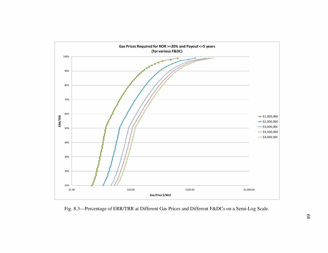
68
Fig. 8.3—Percentage of ERR/TRR at Different Gas Prices and Different F&DCs on a Semi-Log Scale.
10%
20%
30%
40%
50%
60%
70%
80%
90%
100%
$1.00 $10.00 $100.00 $1,000.00
ER
R/T
RR
Gas Price $/Mcf
Gas Prices Required for ROR >=20% and Payout <=5 years
(for various F&DC)
$1,000,000
$2,000,000
$3,000,000
$3,500,000
$4,000,000
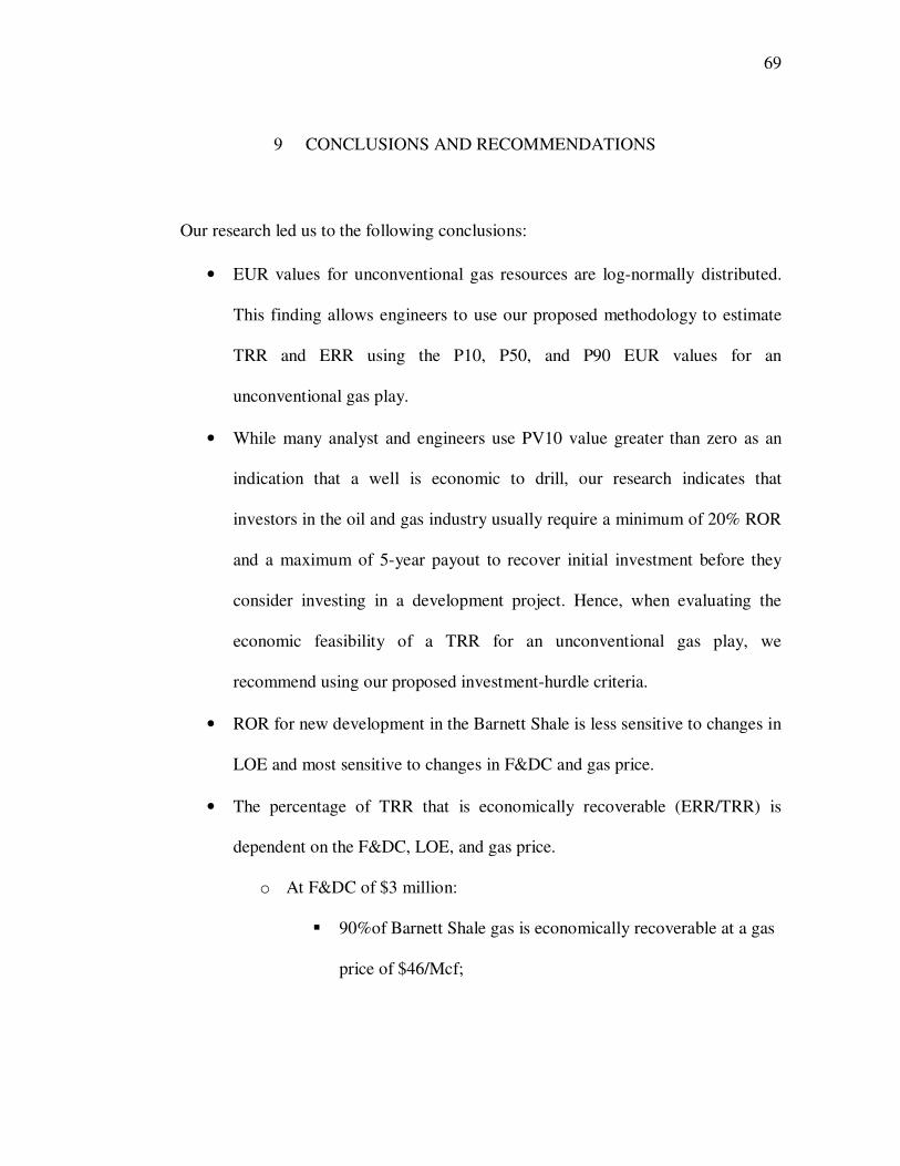
69
9 CONCLUSIONS AND RECOMMENDATIONS
Our research led us to the following conclusions:
• EUR values for unconventional gas resources are log-normally distributed.
This finding allows engineers to use our proposed methodology to estimate
TRR and ERR using the P10, P50, and P90 EUR values for an
unconventional gas play.
• While many analyst and engineers use PV10 value greater than zero as an
indication that a well is economic to drill, our research indicates that
investors in the oil and gas industry usually require a minimum of 20% ROR
and a maximum of 5-year payout to recover initial investment before they
consider investing in a development project. Hence, when evaluating the
economic feasibility of a TRR for an unconventional gas play, we
recommend using our proposed investment-hurdle criteria.
• ROR for new development in the Barnett Shale is less sensitive to changes in
LOE and most sensitive to changes in F&DC and gas price.
• The percentage of TRR that is economically recoverable (ERR/TRR) is
dependent on the F&DC, LOE, and gas price.
o At F&DC of $3 million:
� 90%of Barnett Shale gas is economically recoverable at a gas
price of $46/Mcf;

70
� 75% of Barnett Shale gas is economically recoverable at a gas
price of $24.7/Mcf;
� 50% of Barnett Shale gas is economically recoverable at a gas
price of $9.2/Mcf; and
� 10% of Barnett Shale gas is economically recoverable at a gas
price of $5.2/Mcf.
• Advancements in drilling and completion technologies that can result in
reduction of F&DC will significantly impact the ERR/TRR ratio. At a gas
price of $7.89/Mcf:
o If F&DC is $4 million, approximately 22% of Barnett Shale is
economically recoverable.
o If F&DC is reduced to $2 million, approximately 57% of Barnett
Shale will be economically recoverable.
o If F&DC can be further reduced to $1 million, approximately 75% of
Barnett Shale will be economically recoverable.
• Based on our analysis of the Barnett Shale gas data, the gas price required to
meet our specified investment-hurdle criteria can be approximately estimated
using the following correlation:
Gas Price = (F&DC per Mcf)*(2.77) + (LOE per Mcf)
• Our proposed methodology of using the P10 (10th percentile), P50 (50th
percentile), and P90 (90th percentile) from CDF, to calculate the technically
recoverable resource (TRR) for a gas play, and determine the economically

71
recoverable resource (ERR) as a function of finding and development cost
(F&DC), lease operating expenses (LOE), and gas price can be used to reduce
uncertainties for investments in development of unconventional gas plays.
• Our proposed methodology, selected investment hurdle criteria, and
developed software can be used to quantify TRR and ERR for other
unconventional gas plays based on F&DC, LOE, and gas price.

72
REFERENCES
CME Group, 2010. Henry Hub Natural Gas Futures,
http://www.cmegroup.com/trading/energy/natural-gas/natural-gas.html.
Cook, T. 2005. Calculation of Estimated Ultimate Recovery (EUR) for Wells in
Continuous-Type Oil and Gas Accumulations. U.S. Geological Survey, Denver,
Colorado.
EIA, 2007. Annual Energy Review. US DOE, Washington, DC.
EIA, 2008. Is US Natural Gas Production Increasing?,
http://tonto.eia.doe.gov/energy_in_brief/natural_gas_production.cfm.
EIA, 2010a, Factors Affecting Natural Gas Prices
http://tonto.eia.doe.gov/energyexplained/index.cfm?page=natural_gas_factors_affecti
ng_prices.
EIA, 2010b. Annual Energy Outlook 2010, US DOE, Washington, DC.
Frantz, J.H., Jr., J.R. Williamson, W.K. Sawyer, SPE, D. Johnston, G. Waters, L.P.
Moore, et al. 2005. Evaluating Barnett Shale Production Performance Using an
Integrated Approach, Paper SPE 96917 presented at the SPE Annual Technical
Conference and Exhibition, Dallas, Texas, 9-12 October.
Hayden, J. and Pursell, D, 2005. The Barnett Shale, Visitors Guide to the Hottest Gas
Play in the US. Pickering Energy Partners , Houston, TX.
Herold, J.S, 2009. Global Upstream Performance Review 2006 & 2007, IHS Herold,
Houston, TX.

73
Holditch, S.A. 2006. Tight Gas Sands, SPE Paper 103356, Distinguished Author Series.
Kawata, Y. and Fujita, K. 2001. Some Predictions of Possible Unconventional
Hydrocarbon Availability Until 2100, SPE 68755 presented at the SPE Asia Pacific
Oil and GasConference, Jakarta, Indonesia, April 17–19, 2001.
Mian, M.A., 2002. Project Economics and Decline Analysis Volume I: Deterministic
Models, Tulsa, Oklahoma, Penwell Books.
Navigant Consulting, 2008. North American Natural Gas Supply Assessment. Navigant
Consulting, Houston, TX.
Old, S., 2008. Technology and Economics Affecting Unconventional Reservoir
Development, MS Thesis, Texas A&M University, College Station, TX.
Rogner, H., 1997. An Assessment of World Hydrocarbon Resources, Institute for
Integrated Energy System, An Assessment of World Hydrocarbon Resources, Annual
Review of Energy Environment, 22:217-262.
Securities and Exchange Commission, 2010. Modernization of Oil and Gas Reporting
(SEC Release No. 33-8995, pp. 11-12).
Singh, K. 2006. Basin Analog Approach Answers Characterization Challenges of
Unconventional Gas Potential in Frontier Basins, MS Thesis, Texas A&M
University, College Station, TX.
Texas Railroad Commission, 2010. Barnett Shale Information
http://www.rrc.state.tx.us/barnettshale/index.php.
US Department of Energy (DOE), 2009. Modern Shale Gas Development in the United
States: A Primer. US DOE, Washington, DC.

74
USGS Southwestern Wyoming Province Assessment Team, 2005, Petroleum Systems
and Geologic Assessment of Oil and Gas in the Southwestern Wyoming Province,
Wyoming, Colorado, and Utah, Denver: Geological Survey, Information Services.

75
APPENDIX A
Application input screen:
ECONOMIC EVALUATION OF BARNETT SHALE User Specified Reserves, 10, 50 & 90%-tile
Prices, Escalations, & Operating Costs Initial InvestmentsAre a (Acre ): 60 Well Spacing: 60
Disc. Ra te: 10.00% /ye ar Max. Number of We lls: 1
Royalty Burden: 25.00% Numbe r of Pilot We lls: 0
Probability of Succe ss: 100% % Dry Holes: 5%
Gross Gas Price: $5.60 /Mscf Drill & Complete Cost: $0 /Pilot We ll
Ga s Price Esca lation: 0% /ye ar Drill & Complete Cost: $2,000,000 /Produce r
Cost Esca lation: 0% /ye ar Facilities Cost: $0 /Produce r
Monthly Ope ra ting Cost: $0 /Month/Produce r Dry Hole Cost: $500,000 /Dry Hole
Lea se Ope ra ting Cost: $1.0000 /Mscf
Monthly Facilities Cost: $0 /Month/Produce r Anticipated Reserves DistributionMonthly Facilities Cost: $0.0000 /Mscf (1) Sa n Juan, (2) Bla ck Wa rrior, or (3) Use r Specified:
Fue l & Shrinkage: 6% 3 Use r Specified
W orkover Expense: $0 /Yea r/Produce r
$0 (1) Me dia n We ll or (2) 10, 50, & 90%, (3) Every %-tile
$0 2 10, 50 & 90%-tile
F&DC $1.67 /Mscf
LOE $1.00 /Mscf
T RR 1.70 Bscf Use r Specified Reserves
GP-F&DC-LOE 2.93 /Mscf 10th %tile 25-yr Cum: 0.25 Bscf
Profit Ma rgin 52.34% /Mscf Me dian: 1.50 Bscf
Rese rve s Multiplier: 1.00 90th %tile 25-yr Cum: 4.00 Bscf
Results of Economic Evaluation - User Specified Reserves, 10, 50 & 90%-tile
Discount T iming: Beginning of Period
Forecast: 26 yea rs
Economic Life: 26 yea rs Gross Rese rve s: 1700000.00 Mscf
Payout: 4.7 Ye ars Gross Rese rve s: 1,700,000 Mscf/Producer
ROR: 20% Pea k Rate: 696 Mscf/D
Pea k Rate: 696 Mscf/D /Produce r
Cum Net Profit: $3,513,100
Disc Cum Net Profit: $948,033 Gross Rese rve s: 48,139,548 M^3
Gross Rese rve s: 48,139,548 M^3/Producer
# of Productive We lls: 1 Pea k Rate: 19,704 M^3/D
Pea k Rate: 19,704 M^3/D/Produce r
Initial Investment Breakout - Total Initial Investment $2,000,000
Push T his Button T o Run "Eve ry %-tile" MACRO
RUN

76
APPENDIX B
Assumptions for Detailed Economic Analysis:
Scenario I Assumptions:
o 25-Year well life
o F&DC @ $2 million
o 0% royalty burden
o 100% probability of success
o 0% escalation of gas prices and costs
o 0% fuel and shrinkage
o LOE @ $1.0/Mcf
o 10% annual discount rate
Scenario II Assumptions:
o 25-Year well life
o F&DC @ $2 million
o 25% royalty burden
o 90% probability of success
o 0% escalation of gas prices and costs
o 6% fuel and shrinkage
o LOE @ $1.0/Mcf
o 10% annual discount rate

77
APPENDIX C
VBA Code:
ECORUN()
=ERROR(FALSE)
=SET.NAME("COUNTER",1)
=CALCULATE.NOW()
=WORKBOOK.SELECT("Input","Input")
=CALCULATION(3)
=FORMULA(3,!Macro_Option)
=SELECT(!Old_Cashflow)
=CLEAR(3)
=SELECT(!Old_Prod)
=CLEAR(3)
=SELECT(!View_Area)
=FOR("COUNTER",1,99,1)
= DEFINE.NAME("Cnt",COUNTER)
= CALCULATE.NOW()
= barn()
=NEXT()
=ERROR(FALSE)
=CALCULATE.NOW()
=CALCULATION(1)
78
=SELECT(!$A$1)
=ERROR(TRUE)
=ECHO(TRUE)
=RETURN()
SUB1()
=FORMULA(!New_MACRO_EUR,!MACRO_EUR)
=CALCULATE.NOW()
=SELECT(!New_Cashflow)
=COPY()
=SELECT(!Old_Cashflow)
=PASTE.SPECIAL(3,1,FALSE,FALSE)
=CANCEL.COPY()
=SELECT(!New_Prod)
=COPY()
=SELECT(!Old_Prod)
=PASTE.SPECIAL(3,1,FALSE,FALSE)
=CANCEL.COPY()
=RETURN()
SENS()
=SET.NAME("PARAMCNT",1)
=SET.NAME("SENSCNT",1)
=WORKBOOK.SELECT("Input","Input")

79
=CALCULATION(3)
=SELECT(Orig_Values)
=CLEAR(3)
=FORMULA(Start_Price,Start_Price_Orig)
=FORMULA(Op_Cost,Op_Cost_Orig)
=FORMULA(Gathering__Comprssn,Op_Cost_Mscf_Orig)
=FORMULA(Facilities_Cost,Fac_Cost_Orig)
=FORMULA(Facilities_Cost_Mscf,Fac_Cost_Mscf_Orig)
=FORMULA(G_A_1,G_A_1_Orig)
=FORMULA(G_A_2,G_A_2_Orig)
=FORMULA(Pilot_Inv,DC_1_Orig)
=FORMULA(Producer_Inv,DC_2_Orig)
=FORMULA(Dry_Hole_Inv,Dry_Hole_Orig)
=FORMULA(Facilities_Inv,Facilities_Inv_Orig)
=FORMULA(1,Reserves_Mult)
=FORMULA(1,Reserves_Mult_Orig)
=SELECT(Sens_Price)
=CLEAR(3)
=SELECT(Sens_G_A)
=CLEAR(3)
=SELECT(Sens_Op)
=CLEAR(3)

80
=SELECT(Sens_Water)
=CLEAR(3)
=SELECT(Sens_D_C)
=CLEAR(3)
=SELECT(Sens_Reserves)
=CLEAR(3)
=FOR("PARAMCNT",1,6,1)
= FOR("SENSCNT",1,11,1)
= DEFINE.NAME("Sens_Cnt",SENSCNT)
= DEFINE.NAME("Param_Cnt",PARAMCNT)
= CALCULATE.NOW()
= SELECT(View_Sens)
= FORMULA(OFFSET(Start_Price_Orig,0,2),Start_Price)
= FORMULA(OFFSET(Op_Cost_Orig,0,2),Op_Cost)
=
FORMULA(OFFSET(Op_Cost_Mscf_Orig,0,2),Gathering__Comprssn)
= FORMULA(OFFSET(Fac_Cost_Orig,0,2),Facilities_Cost)
=
FORMULA(OFFSET(Fac_Cost_Mscf_Orig,0,2),Facilities_Cost_Mscf)
= FORMULA(OFFSET(G_A_1_Orig,0,2),G_A_1)
= FORMULA(OFFSET(G_A_2_Orig,0,2),G_A_2)
= FORMULA(OFFSET(DC_1_Orig,0,2),Pilot_Inv)

81
= FORMULA(OFFSET(DC_2_Orig,0,2),Producer_Inv)
= FORMULA(OFFSET(Dry_Hole_Orig,0,2),Dry_Hole_Inv)
= FORMULA(OFFSET(Facilities_Inv_Orig,0,2),Facilities_Inv)
= FORMULA(OFFSET(Reserves_Mult_Orig,0,2),Reserves_Mult)
= CALCULATE.NOW()
= IF(Macro_Option=3,ecorun())
= FORMULA(ROR_Final,OFFSET(Sens_Corner,SENSCNT-
1,1+(PARAMCNT-1)*3))
= NEXT()
=NEXT()
=FORMULA(Start_Price_Orig,Start_Price)
=FORMULA(Op_Cost_Orig,Op_Cost)
=FORMULA(Op_Cost_Mscf_Orig,Gathering__Comprssn)
=FORMULA(Fac_Cost_Orig,Facilities_Cost)
=FORMULA(Fac_Cost_Mscf_Orig,Facilities_Cost_Mscf)
=FORMULA(G_A_1_Orig,G_A_1)
=FORMULA(G_A_2_Orig,G_A_2)
=FORMULA(DC_1_Orig,Pilot_Inv)
=FORMULA(DC_2_Orig,Producer_Inv)
=FORMULA(Dry_Hole_Orig,Dry_Hole_Inv)
=FORMULA(Facilities_Inv_Orig,Facilities_Inv)
=FORMULA(1,Reserves_Mult)

82
=CALCULATE.NOW()
=IF(Macro_Option=3,ecorun())
=CALCULATION(1)
=ERROR(TRUE)
=ECHO(TRUE)
=RETURN()
Loop
End With
ErrHandler:
Resume Next
End Sub
Sub GPRUNALL905010()
Dim ROR As Double
Dim PayOut As Double
Dim GP As Double
Dim LOE As Double
Dim FDCMSCF As Double
Dim EUR As Double
Dim FDC As Double
Dim increment As Double
On Error GoToErrHandler:
With ThisWorkbook.Worksheets("Input")

83
.Cells(22, 7) = 2
increment = 0
FDC = 250000
Do Until FDC > 4000000
GP = 0
ROR = 0
.Cells(11, 8) = FDC
.Cells(10, 3) = GP
ROR = .Cells(37, 3) * 100
PayOut= .Cells(36, 3).Value
Do Until ROR >= 20 And PayOut< 5
GP = GP + 0.1
.Cells(10, 3) = GP
ROR = .Cells(37, 3).Value * 100
PayOut= .Cells(36, 3).Value
Loop
LOE = .Cells(24, 3)
FDCMSCF = .Cells(23, 3)
EUR = .Cells(35, 7) / 1000000
Cells(34 + increment, 22) = GP - LOE - FDCMSCF
Cells(34 + increment, 21) = GP
increment = increment + 1

84
FDC = FDC + 250000
Loop
End With
ErrHandler:
Resume Next
End Sub

85
VITA
Name: Husameddin Saleh A. AlMadani
Born: Edinburgh, Scotland
Permanent Address: P.O. Box 6281
Saudi Aramco
Dhahran, Saudi Arabia 31311
Email: [email protected]
Education: M.S., Petroleum Engineering,
Texas A&M University
College Station, TX, 2010
United States
B. S., Computer Science,
University of Kansas
Lawrence, KS, 2003
United States
Member: International Association for Energy
Economics (IAEE).
Society of Petroleum Engineers (SPE).
Top Related