Download - A Legendre Spectral Collocation Method for the … · A Legendre spectral collocation method is presented for the ... for the solution of a one dimensional fourth order problem. In

Mathematical Modelling and Numerical Analysis M2AN, Vol. 34, No 3, 2000, pp. 637–662

Modelisation Mathematique et Analyse Numerique

A LEGENDRE SPECTRAL COLLOCATION METHODFOR THE BIHARMONIC DIRICHLET PROBLEM

Bernard Bialecki1

and Andreas Karageorghis2

Abstract. A Legendre spectral collocation method is presented for the solution of the biharmonicDirichlet problem on a square. The solution and its Laplacian are approximated using the set ofbasis functions suggested by Shen, which are linear combinations of Legendre polynomials. A Schurcomplement approach is used to reduce the resulting linear system to one involving the approximationof the Laplacian of the solution on the two vertical sides of the square. The Schur complement systemis solved by a preconditioned conjugate gradient method. The total cost of the algorithm is O(N3).Numerical results demonstrate the spectral convergence of the method.

Mathematics Subject Classification. 65N35, 65N22.

Received: March 17, 1999. Revised: November 23, 1999.

1. Introduction

The numerical solution of fourth order problems by spectral methods has been the subject of numerousstudies in recent years. A review of various spectral formulations for fourth order problems in one and twodimensions is given in [1]. Spectral collocation methods have been particularly popular in applications to physicalproblems since, in contrast to spectral Galerkin methods, they do not require the evaluation or approximationof integrals. In [2], spectral collocation methods are studied for the solution of a one dimensional fourthorder problem. In [4], a Legendre spectral collocation method is proposed and analyzed for the biharmonicequation on a square. However, no algorithm for the solution of the corresponding approximate problem isdiscussed. The improvement in the poor conditioning of the spectral discretization of the biharmonic equationis examined in [10]. A Chebyshev spectral collocation method is applied to the driven cavity problem in [16].The application of Chebyshev spectral collocation methods with domain decomposition to the steady-stateNavier-Stokes equations (stream function formulation) in complex geometries is investigated in [11,13]. In [12],a fully conforming Chebyshev spectral collocation scheme is developed for the biharmonic equation in two andthree dimensions. Finally, a spectral collocation method has been applied to fourth order problems in circulardomains in [14]. Further references to the application of spectral methods to fourth order problems can befound in [7] and [3]. The formulation of the biharmonic Legendre spectral collocation problem in this paperand the method of its solution are similar to those developed in [15] and [5] for orthogonal spline collocationwith piecewise Hermite bicubics.

Keywords and phrases. Biharmonic Dirichlet problem, spectral collocation, Schur complement, preconditioned conjugate gradientmethod.

1 Department of Mathematical and Computer Sciences, Colorado School of Mines, Golden, Colorado 80401, U.S.A.e-mail: [email protected] Department of Mathematics and Statistics, University of Cyprus, P.O. Box 537, 1678 Nicosia, Cyprus.

c© EDP Sciences, SMAI 2000

638 B. BIALECKI AND A. KARAGEORGHIS

In this study we consider the biharmonic Dirichlet problem

∆2u = f in Ω, u = ∂u/∂n = 0 on ∂Ω, (1.1)

where ∆ denotes the Laplacian, Ω = (−1, 1)× (−1, 1), ∂Ω is the boundary of Ω, and ∂/∂n is the outer normalderivative on ∂Ω.

In contrast to [4], we use the mixed formulation of (1.1) to obtain approximations to both u and ∆u.Specifically, we set v = ∆u and discretize a coupled pair of Poisson’s equations in u and v using a Legendrespectral collocation method with polynomials of degree ≤ N . As collocation points we take the nodes of theN − 1-point Legendre-Gauss quadrature rather than the Legendre-Gauss-Lobatto points (cf. [4]). Employinga Schur complement approach, we reduce the collocation problem to a Schur complement system involving anapproximation to v on the two vertical sides of ∂Ω and an auxiliary collocation problem for a related biharmonicproblem with v, instead of ∂u/∂n, specified on the two vertical sides of ∂Ω. The matrix in the Schur complementsystem is symmetric and positive definite. (This is not the case when the Legendre-Gauss-Lobatto nodes are usedas collocation points). Consequently, the Schur complement system is solved by the preconditioned conjugategradient (PCG) method. A preconditioner is obtained from the auxiliary collocation problem. We conjecturethat the preconditioner is spectrally equivalent to the Schur complement matrix. The cost of multiplying theSchur complement matrix by a vector and the cost of solving a linear system with the preconditioner are O(N2)each. With the number of PCG iterations proportional to logN , the cost of solving the Schur complementsystem is therefore O(N2 logN). The solution of the auxiliary collocation problem is obtained with cost O(N3)using separation of variables and the solution of a simple generalized eigenvalue problem which reduces to twosymmetric eigenvalue problems with tridiagonal matrices. The total cost of our algorithm is therefore O(N3).The algorithm is well suited for parallel implementation since many of its steps involve independent matrix-vector multiplications. Numerical results demonstrate the spectral convergence rate of the approximations to uand v in the maximum norm. In comparison, the method of [5], the cost of which is O(N2 logN) on an N ×Npartition, yields fourth order approximations to u and v.

In Section 2 we introduce three polynomial spaces, the corresponding basis functions, and collocation matri-ces. In Section 3 we develop an efficient method for solving a 1-d spectral collocation problem. The biharmonicspectral collocation problem and its solution are discussed in Sections 4 and 5, respectively. Numerical resultsand conclusions are given in Sections 6 and 7, respectively.

2. Preliminaries

ForN ≥ 4, let ξiN−1i=1 and respectively wiN−1

i=1 be the nodes and weights of the N−1-point Legendre-Gaussquadrature on (−1, 1), and let

D = diag(w1, . . . , wN−1). (2.1)

For p and q defined on ξiN−1i=1 , let

〈p, q〉 =N−1∑i=1

wi(pq)(ξi). (2.2)

It follows from the exactness property of the Legendre-Gauss quadrature that

〈p, q〉 =∫ 1

−1

(pq)(x) dx, pq ∈ P2N−3, (2.3)

A LEGENDRE SPECTRAL COLLOCATION METHOD FOR THE BIHARMONIC DIRICHLET PROBLEM 639

where Pk denotes the set of polynomials of degree ≤ k on (−1, 1). Lemma 3.1 in [8] implies also that

−〈p′′, q〉 =∫ 1

−1

(p′q′)(x) dx− p′q|1−1 + CNp(N)q(N), p, q ∈ PN , (2.4)

where CN denotes a generic positive constant that may depend on N .Let

P 0N = p ∈ PN : p(±1) = 0, P 00

N = p ∈ P 0N : p′(±1) = 0.

(Note that the dimensions of PN , P 0N , and P 00

N are N + 1, N − 1, and N − 3, respectively.) Following (2.7) and(3.4) of [17], we introduce the basis φkNk=2 for P 0

N and the basis ψkNk=4 for P 00N with

φk(x) = ck[Lk−2(x)− Lk(x)], k = 2, . . . , N, (2.5)

ψk(x) = dk [Lk−4(x) + akLk−2(x) + bkLk(x)] , k = 4, . . . , N, (2.6)

where Lk(x) is the kth degree Legendre polynomial normalized by∫ 1

−1L2k(x) dx = 2/(2k + 1), and

ck =1√

4k − 2, dk =

1√2(2k − 5)2(2k − 3)

, ak = −22k − 32k − 1

, bk =2k − 52k − 1

. (2.7)

Augmenting the basis ψkNk=4 for P 00N by ψ2, ψ3 ∈ P 0

N such that

ψ′2(−1) = 1, ψ′2(1) = 0, ψ′3(−1) = 0, ψ′3(1) = 1, (2.8)

we obtain the basis ψkNk=2 for P 0N . Since ψ2, ψ3 ∈ P 0

N and since φkNk=2 is a basis for P 0N ,

ψ2(x) =N∑k=2

αkφk(x), ψ3(x) =N∑k=2

βkφk(x), (2.9)

for some αkNk=2 and βkNk=2. Later we will consider a particular choice of αkNk=2 and

βk = (−1)k−1αk, k = 2, . . . , N. (2.10)

Using (2.5)–(2.7) it is easy to verify that

ψk(x) = dk[c−1k−2φk−2(x)− bkc−1

k φk(x)], k = 4, . . . , N. (2.11)

Thus it follows from (2.9)–(2.11) that

[ψ2(x), . . . , ψN (x)] = [φ2(x), . . . , φN (x)]M, (2.12)

where the nonsingular matrix M has the structure shown in Figure 1.Augmenting the basis ψkNk=2 for P 0

N by

ψ0(x) =12

[L0(x)− L1(x)], ψ1(x) =12

[L0(x) + L1(x)], (2.13)


× −× ×× × ×× −× × ×...

.... . .

. . .× −× × ×× × ×× −× ×

Figure 1. Structure of the (N − 1)× (N − 1) matrix M .

we obtain the basis ψkNk=0 for PN , where

ψ0(−1) = 1, ψ0(1) = 0, ψ1(−1) = 0, ψ1(1) = 1. (2.14)

Let

Aψ = (−ψ′′k(ξi))N−1,Ni=1,k=2, Bψ = (ψk(ξi))

N−1,Ni=1,k=2, (2.15)

Aψ,t = (−ψ′′k(ξi))N−1,1i=1,k=0, Bψ,t = (ψk(ξi))

N−1,1i=1,k=0, (2.16)

Aφ = (−φ′′k(ξi))N−1,Ni=1,k=2, Bφ = (φk(ξi))

N−1,Ni=1,k=2, (2.17)

where i and k are the row and column indices, respectively. Clearly, (2.16) and (2.13) imply

Aψ,t = 0. (2.18)

It follows from (2.15), (2.17), and (2.12) that

Aψ = AφM, Bψ = BφM. (2.19)

Let

A′φ = BTφDAφ, B′φ = BTφDBφ, (2.20)

where D is given by (2.1). Clearly, B′φ is symmetric and positive definite.

Lemma 2.1. The matrix B′φ has the structure shown in Figure 2 and

A′φ = diag(1, . . . , 1,×), (2.21)

where the element × is positive.

Proof. Equations (2.20), (2.17), and (2.1), imply that the coefficients of B′φ = (b′k,l)Nk,l=2 and A′φ = (a′k,l)

Nk,l=2

are given by the formulas

b′k,l =N−1∑i=1

wi(φkφl)(ξi), a′k,l = −N−1∑i=1

wi(φ′′kφl)(ξi), k, l = 2, . . . , N.


× ×× ×

× × ×. . .

. . .. . .

× × ×× ×× ×

Figure 2. Structure of the (N − 1)× (N − 1) matrix B′φ.

Hence it follows from (2.2), (2.3), and Lemma 2.1 in [17] that in order to prove both claims it suffices to showthat

b′N,N−1 = 0, a′N,N > 0.

For N odd (N − 1 even), we have

bN,N−1 =(N−1)/2∑i=1

wi(φNφN−1)(ξi) +(N−1)/2∑i=1

wi(φNφN−1)(−ξi) = 0,

where the first identity follows from the symmetry of wiN−1i=1 and the antisymmetry of ξiN−1

i=1 about 0, andthe second identity follows from (φNφN−1)(−x) = −(φNφN−1)(x) which is a consequence of (2.5) and (2.7).

For N even (N − 1 odd), using arguments similar to those for odd N , we have

bN,N−1 =(N−2)/2∑i=1

wi(φNφN−1)(ξi) +(N−2)/2∑i=1

wi(φNφN−1)(−ξi) + (φNφN−1)(0)w1+(N−2)/2 = 0,

where in the last step we also used φN−1(0) = 0 which follows from (2.5) and Lk(0) = 0 for odd k.Finally, (2.4) applied to p = q = φN and (2.2) imply a′N,N > 0.

Let

A′ψ = BTφDAψ, B′ψ = BTφDBψ. (2.22)

Then it follows from (2.19) and (2.20) that

A′ψ = A′φM, B′ψ = B′φM. (2.23)

Let

B′ψ,t = BTφDBψ,t. (2.24)

Then (2.17), (2.1), (2.16), (2.2), (2.3), (2.5), (2.13), and orthogonality of the Legendre polynomials imply thatthat B′ψ,t has the structure shown in Figure 3. Let

Aψ,e = [Aψ,t|Aψ], Bψ,e = [Bψ,t|Bψ], (2.25)


× ×× ×0 0...

...0 0

Figure 3. Structure of the (N − 1)× 2 matrix B′ψ,t.

and let

A′ψ,e = BTφDAψ,e, B′ψ,e = BTφDBψ,e. (2.26)

Then it follows from (2.18), (2.24), (2.22), and (2.23) that

A′ψ,e = [0|A′φM ], B′ψ,e = [B′ψ,t|B′φM ]. (2.27)

3. 1-D Spectral Collocation Problem

Solving the biharmonic problem requires the solution of the following 1-d spectral collocation problem.For given λ > 0, giN−1

i=1 , fiN−1i=1 , α, and β, consider the problem of finding p ∈ P 0

N and q ∈ PN such that

p(ξi)− λp′′(ξi) + λq(ξi) = gi, i = 1, . . . , N − 1, (3.1)q(ξi)− λq′′(ξi) = fi, i = 1, . . . , N − 1. (3.2)

p′(−1) = α, p′(1) = β. (3.3)

Theorem 3.1. For λ > 0, there exist unique p ∈ P 0N and q ∈ PN satisfying (3.1)–(3.3).

Proof. Since in (3.1)–(3.3), the number of unknowns, which is 2N , is equal to the number of equations, weassume gi = fi = 0, i = 1, . . . , 2N , α = β = 0 and show that p = q = 0. Taking the inner product 〈·, ·〉 with qon both sides of (3.1) and with p on both sides of (3.2), respectively, we obtain

〈p, q〉 − λ〈p′′, q〉+ λ〈q, q〉 = 0,〈q, p〉 − λ〈q′′, p〉 = 0. (3.4)

It follows from (2.4) and p(±1) = p′(±1) = 0 that 〈p′′, q〉 = 〈q′′, p〉. Hence (3.4) gives 〈q, q〉 = 0, which implies

q(ξi) = 0, i = 1, . . . , N − 1. (3.5)

From (3.2) and (3.5), we have q′′(ξi) = 0, i = 1, . . . , N − 1, which yields q′′ = 0 since q′′ ∈ PN−2. Thus q ∈ P1

and hence (3.5) and N ≥ 3 imply q = 0.From (3.1) and (3.5), we have

〈p, p〉 − λ〈p′′, p〉 = 0.

Since, by (2.4), −〈p′′, p〉 ≥ 0, it follows that 〈p, p〉 = 0. Thus p(ξi) = 0, i = 1, . . . , N − 1, which along withp(±1) = 0 implies p = 0.


In the remainder of this section we consider a matrix-vector form of (3.1)–(3.3), assuming that ψkNk=2 andψkNk=0 are respectively bases for P 0

N and PN introduced in Section 2. Substituting

p(x) =N∑k=2

pkψk(x), q(x) =N∑k=0

qkψk(x),

into (3.1)–(3.3), and using (2.15), (2.16), (2.25), (2.8), and ψ′k(±1) = 0, k = 4, . . . , N , we obtain

(Bψ + λAψ)~p+ λBψ,e~qe = ~g, (Bψ,e + λAψ,e)~qe = ~f, p2 = α, p3 = β, (3.6)

where

~p = [p2, . . . , pN ]T , ~qe = [q0, . . . , qN ]T , (3.7)

~g = [g1, . . . , gN−1]T , ~f = [f1, . . . , fN−1]T .

Multiplying the first two equations of (3.6) by BTφD, with Bφ and D defined in (2.17) and (2.1), respectively,and using (2.22), (2.26), we obtain

(B′ψ + λA′ψ)~p+ λB′ψ,e~qe = ~gφ, (B′ψ,e + λA′ψ,e)~qe = ~fφ, p2 = α, p3 = β, (3.8)

where

~gφ = BTφD~g,~fφ = BTφD

~f. (3.9)

Rewriting ~qe of (3.7) as

~qe = [q0, q1, ~q]T , ~q = [q2, . . . , qN ]T ,

and using (2.23), (2.27), (2.8), ψ′k(±1) = 0, k = 4, . . . , N , and (2.12), we obtain

(B′φ + λA′φ)~pM + λB′φ~qM + λB′ψ,t[q0, q1]T = ~gφ,

(B′φ + λA′φ)~qM +B′ψ,t[q0, q1]T = ~fφ, (3.10)

Cφ~pM = [α, β]T ,

where

~pM = M~p, ~qM = M~q, (3.11)

and

Cφ =[φ′2(−1) φ′3(−1) . . . φ′N (−1)φ′2(1) φ′3(1) . . . φ′N (1)

].

Equations (3.10) can be rewritten as

S11 [~pM , ~qM ]T + S12 [q0, q1]T =[~gφ, ~fφ

]T, (3.12)

S21 [~pM , ~qM ]T = [α, β]T , (3.13)


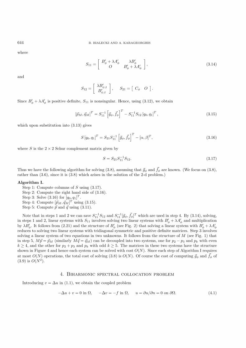
where

S11 =[B′φ + λA′φ λB′φ

O B′φ + λA′φ

], (3.14)

and

S12 =[λB′ψ,tB′ψ,t

], S21 =

[Cφ O

].

Since B′φ + λA′φ is positive definite, S11 is nonsingular. Hence, using (3.12), we obtain

[~pM , ~qM ]T = S−111

[~gφ, ~fφ

]T− S−1

11 S12 [q0, q1]T , (3.15)

which upon substitution into (3.13) gives

S [q0, q1]T = S21S−111

[~gφ, ~fφ

]T− [α, β]T , (3.16)

where S is the 2× 2 Schur complement matrix given by

S = S21S−111 S12. (3.17)

Thus we have the following algorithm for solving (3.8), assuming that ~gφ and ~fφ are known. (We focus on (3.8),rather than (3.6), since it is (3.8) which arises in the solution of the 2-d problem.)

Algorithm I.Step 1: Compute columns of S using (3.17).Step 2: Compute the right hand side of (3.16).Step 3: Solve (3.16) for [q0, q1]T .Step 4: Compute [~pM , ~qM ]T using (3.15).Step 5: Compute ~p and ~q using (3.11).

Note that in steps 1 and 2 we can save S−111 S12 and S−1

11 [~gφ, ~fφ]T which are used in step 4. By (3.14), solving,in steps 1 and 2, linear systems with S11 involves solving two linear systems with B′φ + λA′φ and multiplicationby λB′φ. It follows from (2.21) and the structure of B′φ (see Fig. 2) that solving a linear system with B′φ + λA′φreduces to solving two linear systems with tridiagonal symmetric and positive definite matrices. Step 3 involvessolving a linear system of two equations in two unknowns. It follows from the structure of M (see Fig. 1) thatin step 5, M~p = ~pM (similarly M~q = ~qM ) can be decoupled into two systems, one for p2 − p3 and pk with evenk ≥ 4, and the other for p2 + p3 and pk with odd k ≥ 5. The matrices in these two systems have the structureshown in Figure 4 and hence each system can be solved with cost O(N). Since each step of Algorithm I requiresat most O(N) operations, the total cost of solving (3.8) is O(N). Of course the cost of computing ~gφ and ~fφ of(3.9) is O(N2).

4. Biharmonic spectral collocation problem

Introducing v = ∆u in (1.1), we obtain the coupled problem

−∆u+ v = 0 in Ω, −∆v = −f in Ω, u = ∂u/∂n = 0 on ∂Ω. (4.1)


× ×× × ×× × ×...

. . .. . .

× × ×× ×

Figure 4. Structure of the matrices in decoupled systems for M~p = ~pM .

The Legendre spectral collocation problem corresponding to (4.1) consists of finding U ∈ P 00N ⊗ P 00

N andV ∈ PN ⊗ PN such that

−∆U(ξi, ξj) + V (ξi, ξj) = 0, −∆V (ξi, ξj) = −f(ξi, ξj), i, j = 1, . . . , N − 1, (4.2)

and

V (a, b) = Vy(a, b) = 0, a, b = ±1. (4.3)

We prove existence and uniqueness of the solution to (4.2)–(4.3) following the proof of Theorem 5.1 in [15]. Tothis end, we require an additional notation and two lemmas. For p and q defined on (x, y) : x, y ∈ ξiN−1

i=1 ,let

〈〈p, q〉〉 =N−1∑i=1

N−1∑j=1

wiwj(pq)(ξi, ξj). (4.4)

Lemma 4.1. If U ∈ P 00N ⊗ P 00

N and V ∈ PN ⊗ PN , then

〈〈−∆U, V 〉〉 = 〈〈U,−∆V 〉〉.

Proof. Since Ux(a, y) = 0, a = ±1, y ∈ [−1, 1], using (2.4), we have

〈〈−Uxx, V 〉〉 = −N−1∑j=1

wj〈Uxx(·, ξj), V (·, ξj)〉

=N−1∑j=1

wj

[∫ 1

−1

(UxVx)(x, ξj) dx+ CN

(∂NU

∂xN∂NV

∂xN

)(·, ξj)

].

In a similar way, using (2.4) and U(a, y) = 0, a = ±1, y ∈ [−1, 1], we obtain

〈〈−Vxx, U〉〉 =N−1∑j=1

wj

[∫ 1

−1

(VxUx)(x, ξj) dx+ CN

(∂NV

∂xN∂NU

∂xN

)(·, ξj)

].

Therefore 〈〈−Uxx, V 〉〉 = 〈〈U,−Vxx〉〉. By symmetry in x and y we also have 〈〈−Uyy, V 〉〉 = 〈〈U,−Vyy〉〉. Hencethe desired result follows.


Lemma 4.2. If V ∈ PN ⊗ PN satisfies

V (a, b) = Vy(a, b) = 0, a, b = ±1, (4.5)

then

〈〈Vxx, Vyy〉〉 = 〈〈V, Vxxyy〉〉. (4.6)

Proof. Applying (2.4) with respect to y to the left-hand side of (4.6), we have

〈〈Vxx, Vyy〉〉 =N−1∑i=1

wi〈Vyy(ξi, ·), Vxx(ξn, ·)〉

= −N−1∑i=1

wi

∫ 1

−1

(VyVxxy)(ξi, y) dy

+N−1∑i=1

wi(VyVxx)(ξi, y)|y=1y=−1 − CN

N−1∑i=1

wi

(∂NV

∂yN∂N+2V

∂yN∂x2

)(ξi, ·).

(4.7)

Applying (2.4) to the second term on the right-hand side in (4.7), we obtain, for y = ±1,

N−1∑i=1

wi(VyVxx)(ξi, y) = 〈Vxx(·, y), Vy(·, y)〉

= −∫ 1

−1

(VxVyx)(x, y) dx+ (VxVy)(x, y)|x=1x=−1 − CN

(∂NV

∂xN∂N+1V

∂xN∂y

)(·, y).

(4.8)

Applying (2.4) to the first term on the right-hand side in (4.8), we obtain, for y = ±1,

−∫ 1

−1

(VyxVx)(x, y) dx =N−1∑i=1

wi(VyxxV )(ξi, y)− (VyxV )(x, y)|x=1x=−1 + CN

N−1∑i=1

wi

(∂N+1V

∂xN∂y

∂NV

∂xN

)(·, y). (4.9)

Substituting (4.9) into (4.8) and using (4.5), we have

N−1∑i=1

wi(VyVxx)(ξi, y) =N−1∑i=1

wi(VyxxV )(ξi, y), y = ±1. (4.10)

Applying (2.4) with respect to y to the right-hand side of (4.6), we also obtain

〈〈V, Vxxyy〉〉 =N−1∑i=1

wi〈Vxxyy(ξi, ·), V (ξi, ·)〉

= −N−1∑i=1

wi

∫ 1

−1

(VxxyVy)(ξi, y) dy

+N−1∑i=1

wi(VxxyV )(ξi, y)|y=1y=−1 − CN

N−1∑i=1

wi∂N+2V

∂yN∂x2

∂NV

∂yN(ξi, .)·

(4.11)

Comparing the right-hand sides of (4.7) and (4.11), and using (4.10), we obtain (4.6).

Theorem 4.3. There exist unique U ∈ P 00N ⊗ P 00

N and V ∈ PN ⊗ PN satisfying (4.2)–(4.3).


Proof. Since the number of unknown coefficients in U and V , which is N2 − 4N + 10, is equal to the numberof equations in (4.2)–(4.3), it suffices to show that if U and V satisfy (4.2)–(4.3) with f = 0, then U = V = 0.

Taking the inner product 〈〈·, ·〉〉 with V on both sides of the first equation in (4.2), we obtain

〈〈−∆U, V 〉〉 + 〈〈V, V 〉〉 = 0. (4.12)

Similarly, taking the inner product 〈〈·, ·〉〉 with U on both sides of the second equation in (4.2), we obtain

〈〈−∆V,U〉〉 = 0. (4.13)

From (4.12), (4.13), and Lemma 4.1, we have 〈〈V, V 〉〉 = 0, which implies

V (ξi, ξj) = 0, i, j = 1, . . . , N − 1. (4.14)

Thus, by the first equation in (4.2),

−∆U(ξi, ξj) = 0, i, j = 1, . . . , N − 1.

Using this equation, (2.4) with respect to x and y, and U = 0 on ∂Ω, we have

0 = 〈〈−∆U,U〉〉 = −N−1∑j=1

wj〈Uxx(·, ξj), U(·, ξj)〉 −N−1∑i=1

wi〈Uyy(ξi, ·), U(ξi, ·)〉

≥N−1∑j=1

wj

∫ 1

−1

U2x(x, ξj) dx+

N−1∑i=1

wi

∫ 1

−1

U2y (ξi, y) dy,

which along with U = 0 on ∂Ω implies that U = 0 on the horizontal and vertical lines passing through thepoints (ξi, ξj), i, j = 1, . . . , N−1. This and U = 0 on ∂Ω imply further that U = 0 on all horizontal and verticallines passing through Ω, and hence U = 0.

To show that V = 0, we use the second equation in (4.2) (with f = 0), Lemma 4.2 , and (4.14) to obtain

0 = 〈〈∆V,∆V 〉〉 = 〈〈Vxx, Vxx〉〉+ 2〈〈Vxx, Vyy〉〉+ 〈〈Vyy , Vyy〉〉= 〈〈Vxx, Vxx〉〉+ 2〈〈V, Vxxyy〉〉+ 〈〈Vyy , Vyy〉〉 = 〈〈Vxx, Vxx〉〉+ 〈〈Vyy, Vyy〉〉.

Hence

Vxx(ξi, ξj) = Vyy(ξi, ξj) = 0, i, j = 1, . . . , N − 1,

which along with (4.14) implies that V = 0 on the horizontal and vertical lines passing through the points(ξi, ξj), i, j = 1, . . . , N − 1. This and V (a, b) = 0, a, b = ±1, imply in turn that V = 0 on ∂Ω. Therefore, V = 0on all horizontal and vertical lines passing through Ω, and hence V = 0.

Let the functions ψkNk=0 be as in Section 2 with αkNk=2 of (2.9) yet to be specified and βkNk=2 as in(2.10). Since ψkNk=4, ψkNk=2, and ψkNk=0 form bases for P 00

N , P 0N , and PN , respectively, and since ψ0, ψ1

and ψ2, ψ3 satisfy (2.14) and (2.8), respectively, for U ∈ P 00N ⊗ P 00

N and V ∈ PN ⊗ PN satisfying (4.3), we have

U(x, y) =N∑k=2

N∑l=4

uk,lψk(x)ψl(y) (4.15)

with

u2,l = u3,l = 0, l = 4, . . . , N, (4.16)


and

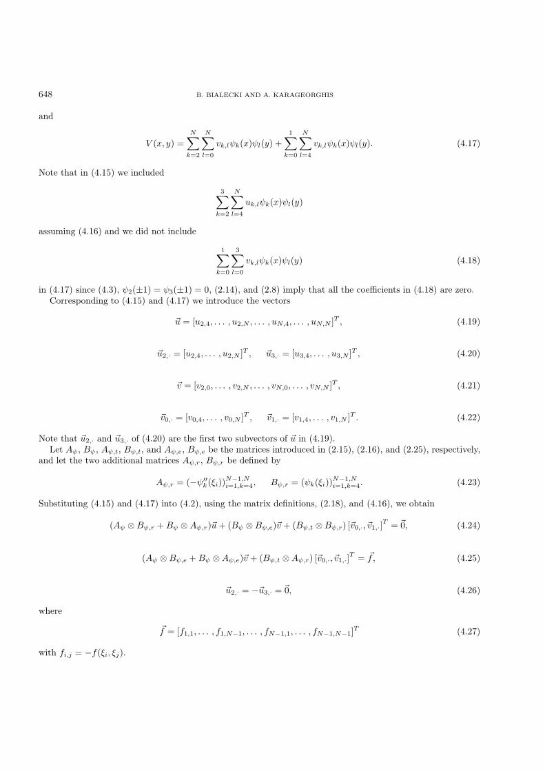
V (x, y) =N∑k=2

N∑l=0

vk,lψk(x)ψl(y) +1∑k=0

N∑l=4

vk,lψk(x)ψl(y). (4.17)

Note that in (4.15) we included

3∑k=2

N∑l=4

uk,lψk(x)ψl(y)

assuming (4.16) and we did not include

1∑k=0

3∑l=0

vk,lψk(x)ψl(y) (4.18)

in (4.17) since (4.3), ψ2(±1) = ψ3(±1) = 0, (2.14), and (2.8) imply that all the coefficients in (4.18) are zero.Corresponding to (4.15) and (4.17) we introduce the vectors

~u = [u2,4, . . . , u2,N , . . . , uN,4, . . . , uN,N ]T , (4.19)

~u2,· = [u2,4, . . . , u2,N ]T , ~u3,· = [u3,4, . . . , u3,N ]T , (4.20)

~v = [v2,0, . . . , v2,N , . . . , vN,0, . . . , vN,N ]T , (4.21)

~v0,· = [v0,4, . . . , v0,N ]T , ~v1,· = [v1,4, . . . , v1,N ]T . (4.22)

Note that ~u2,· and ~u3,· of (4.20) are the first two subvectors of ~u in (4.19).Let Aψ, Bψ, Aψ,t, Bψ,t, and Aψ,e, Bψ,e be the matrices introduced in (2.15), (2.16), and (2.25), respectively,

and let the two additional matrices Aψ,r, Bψ,r be defined by

Aψ,r = (−ψ′′k(ξi))N−1,Ni=1,k=4, Bψ,r = (ψk(ξi))

N−1,Ni=1,k=4. (4.23)

Substituting (4.15) and (4.17) into (4.2), using the matrix definitions, (2.18), and (4.16), we obtain

(Aψ ⊗Bψ,r +Bψ ⊗Aψ,r)~u+ (Bψ ⊗Bψ,e)~v + (Bψ,t ⊗Bψ,r) [~v0,·, ~v1,·]T = ~0, (4.24)

(Aψ ⊗Bψ,e +Bψ ⊗Aψ,e)~v + (Bψ,t ⊗Aψ,r) [~v0,·, ~v1,·]T = ~f, (4.25)

~u2,· = −~u3,· = ~0, (4.26)

where

~f = [f1,1, . . . , f1,N−1, . . . , fN−1,1, . . . , fN−1,N−1]T (4.27)

with fi,j = −f(ξi, ξj).


5. Solving the biharmonic spectral collocation problem

In this section we present a method for solving (4.24)–(4.26).

5.1. Formulation of the method

Let Ik be the k × k identity matrix. Multiplying (4.24) and (4.25) by BTφD ⊗ BTφD, (4.26) by BTψ,rDBψ,rand using (2.22)–(2.24), (2.26), we obtain

(A′φ ⊗B′ψ,r +B′φ ⊗A′ψ,r)(M ⊗ IN−3)~u+ (B′φ ⊗B′ψ,e)(M ⊗ IN+1)~v + (B′ψ,t ⊗B′ψ,r) [~v0,·, ~v1,·]T = ~0, (5.1)

(A′φ ⊗B′ψ,e +B′φ ⊗A′ψ,e)(M ⊗ IN+1)~v + (B′ψ,t ⊗A′ψ,r) [~v0,·, ~v1,·]T = ~fφ, (5.2)

BTψ,rDBψ,r~u2,· = −BTψ,rDBψ,r~u3,· = ~0, (5.3)

where

A′ψ,r = BTφDAψ,r, B′ψ,r = BTφDBψ,r, (5.4)

~fφ = (BTφD ⊗BTφD)~f. (5.5)

Lemma 5.1. The matrix of the linear system (5.1)–(5.3) is nonsingular.

Proof. Clearly, Bψ of (2.15) is nonsingular since p = 0 is the only p ∈ P 0N such that p(ξi) = 0, i = 1, . . . , N − 1.

Hence the rank of the (N − 1) × (N − 3) matrix Bψ,r of (4.23) is N − 3. This implies nonsingularity of the(N−3)×(N−3) matrix BTψ,rDBψ,r since BTψ,rDBψ,r ~w = ~0 yields ~wT (D1/2Bψ,r)TD1/2Bψ,r ~w = 0, D1/2Bψ,r ~w =~0, Bψ,r ~w = ~0, and ~w = ~0. The desired result follows now from the nonsingularity of BTφD, BTψ,rDBψ,r, and thematrix in (4.24)–(4.26), which is guaranteed by the uniqueness of the solution to (4.2)–(4.3).

Equations (5.1)–(5.3) can be written as

S11 [~u,~v]T + S12 [~v0,·, ~v1,·]T =

[~0, ~fφ

]T, (5.6)

S21 [~u,~v]T = ~0, (5.7)

where

S11 =[

(A′φ ⊗B′ψ,r +B′φ ⊗A′ψ,r)(M ⊗ IN−3) (B′φ ⊗B′ψ,e)(M ⊗ IN+1)O (A′φ ⊗B′ψ,e +B′φ ⊗A′ψ,e)(M ⊗ IN+1)

], (5.8)

S12 =[B′ψ,t ⊗B′ψ,rB′ψ,t ⊗A′ψ,r

], (5.9)

S21 =[BTψ,rDBψ,r O O

O −BTψ,rDBψ,r O

]. (5.10)

Note that the two blocks BTψ,rDBψ,r in S21 of (5.10) correspond to multiplications by ~u2,· and ~u3,· in (5.3).


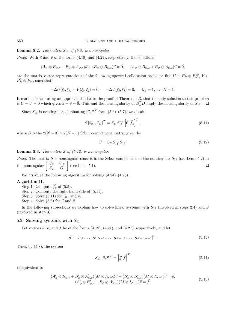
Lemma 5.2. The matrix S11 of (5.8) is nonsingular.

Proof. With ~u and ~v of the forms (4.19) and (4.21), respectively, the equations

(Aψ ⊗Bψ,r +Bψ ⊗Aψ,r)~u+ (Bψ ⊗Bψ,e)~v = ~0, (Aψ ⊗Bψ,e +Bψ ⊗Aψ,e)~v = ~0,

are the matrix-vector representations of the following spectral collocation problem: find U ∈ P 0N ⊗ P 00

N , V ∈P 0N ⊗ PN , such that

−∆U(ξi, ξj) + V (ξi, ξj) = 0, −∆V (ξi, ξj) = 0, i, j = 1, . . . , N − 1.

It can be shown, using an approach similar to the proof of Theorem 4.3, that the only solution to this problemis U = V = 0 which gives ~u = ~v = ~0. This and the nonsingularity of BTφD imply the nonsingularity of S11.

Since S11 is nonsingular, eliminating [~u,~v]T from (5.6)–(5.7), we obtain

S [~v0,·, ~v1,·]T = S21S

−111

[~0, ~fφ

]T, (5.11)

where S is the 2(N − 3)× 2(N − 3) Schur complement matrix given by

S = S21S−111 S12. (5.12)

Lemma 5.3. The matrix S of (5.12) is nonsingular.

Proof. The matrix S is nonsingular since it is the Schur complement of the nonsingular S11 (see Lem. 5.2) in

the nonsingular[S11 S12

S21 O

](see Lem. 5.1).

We arrive at the following algorithm for solving (4.24)–(4.26).

Algorithm II.Step 1: Compute ~fφ of (5.5).Step 2: Compute the right-hand side of (5.11).Step 3: Solve (5.11) for ~v0,· and ~v1,·.Step 4: Solve (5.6) for ~u and ~v.

In the following subsections we explain how to solve linear systems with S11 (involved in steps 2,4) and S(involved in step 3).

5.2. Solving systems with S11

Let vectors ~u, ~v, and ~f be of the forms (4.19), (4.21), and (4.27), respectively, and let

~g = [g1,1, . . . , g1,N−1, . . . , gN−1,1, . . . , gN−1,N−1]T . (5.13)

Then, by (5.8), the system

S11 [~u,~v]T =[~g, ~f]T

(5.14)

is equivalent to

(A′φ ⊗B′ψ,r +B′φ ⊗A′ψ,r)(M ⊗ IN−3)~u+ (B′φ ⊗B′ψ,e)(M ⊗ IN+1)~v = ~g,

(A′φ ⊗B′ψ,e +B′φ ⊗A′ψ,e)(M ⊗ IN+1)~v = ~f.(5.15)


We rewrite (5.15) as

(A′φ ⊗B′ψ +B′φ ⊗A′ψ)(M ⊗ IN−1)~ue + (B′φ ⊗B′ψ,e)(M ⊗ IN+1)~v = ~g,

(A′φ ⊗B′ψ,e +B′φ ⊗A′ψ,e)(M ⊗ IN+1)~v = ~f,

BTψDBψ~u·,2 = ~α, −BTψDBψ~u·,3 = ~β,

(5.16)

where

~ue = [u2,2, u2,3, . . . , u2,N , . . . , uN,2, uN,3, . . . , uN,N ]T , (5.17)

~u·,2 = [u2,2, u3,2 . . . , uN,2]T , ~u·,3 = [u2,3, u3,3 . . . , uN,3]T , (5.18)

and

~α = [α2, . . . , αN ]T , ~β = [β2, . . . , βN ]T . (5.19)

Note that ~ue in (5.17) is an extension of ~u in (4.19) with the components of ~u·,2 and ~u·,3 in (5.18) added to ~u.Consequently, (5.16) is obtained from (5.15) by replacing ~u, A′ψ,r, and B′ψ,r with ~ue, A′ψ, and B′ψ, respectively,and by adding two additional equations for ~u·,2 and ~u·,3.

Note also that (5.14) (equivalently (5.15)) is a special case of (5.16) with ~α = ~β = ~0.

Lemma 5.4. The matrix of the linear system (5.16) is nonsingular.

Proof. The desired result follows easily from nonsingularity of BTψDBψ and S11.

Since A′φ and B′φ of (2.20) are symmetric and A′φ is positive definite, it follows from Corollary 8.7.2 in [9]that there exists a real nonsingular (N − 1)× (N − 1) matrix Z and real

Λ = diag(λ2, . . . , λN ) (5.20)

such that

ZTA′φZ = IN−1, ZTB′φZ = Λ. (5.21)

Since Z of (5.21) and M of (2.12) are nonsingular, (5.16) is equivalent to

(ZT ⊗ IN−1)(A′φ ⊗B′ψ +B′φ ⊗A′ψ)(Z ⊗ IN−1)~u′e + (ZT ⊗ IN−1)(B′φ ⊗B′ψ,e)(Z ⊗ IN+1)~v′ = ~g′,

(ZT ⊗ IN−1)(A′φ ⊗B′ψ,e +B′φ ⊗A′ψ,e)(Z ⊗ IN+1)~v′ = ~f ′, (5.22)

ZTM−TBTψDBψM−1Z~u′·,2 = ~α′, −ZTM−TBTψDBψM−1Z~u′·,3 = ~β′,

where ~u′e and ~v′ are such that

~ue = (W ⊗ IN−1)~u′e, ~v = (W ⊗ IN+1)~v′, ~u·,2 = W~u′·,2, ~u·,3 = W~u′·,3, (5.23)

with

W = M−1Z, (5.24)


and

~g′ = (ZT ⊗ IN−1)~g, ~f ′ = (ZT ⊗ IN−1)~f, ~α′ = WT ~α, ~β′ = WT ~β. (5.25)

The vectors ~u′e, ~v′, ~u′·,2, ~u′·,3, ~g′, ~f ′, and ~α′, ~β′ have the same forms as ~ue of (5.17), ~v of (4.21), ~u·,2, ~u·,3 of (5.18),~g of (5.13), ~f of (4.27), and ~α, ~β of (5.19), respectively. In the following, the components of the primed vectorsare denoted by the primed letters corresponding to the unprimed vectors. For example,

~u′e = [u′2,2, u′2,3, . . . , u

′2,N , . . . , u

′N,2, u

′N,3, . . . , u

′N,N ]T .

Using (2.19), (2.20), and (5.21) in (5.22), we obtain

(IN−1 ⊗B′ψ + Λ⊗A′ψ)~u′e + (Λ⊗B′ψ,e)~v′ = ~g′,

(IN−1 ⊗B′ψ,e + Λ⊗A′ψ,e)~v′ = ~f ′,

Λ~u′·,2 = ~α′,−Λ~u′·,3 = ~β′,

which, by (5.20), become

(B′ψ + λkA′ψ)~u′k,· + λkB

′ψ,e~v

′k,· = ~g′k,·, (B

′ψ,e + λkA

′ψ,e)~v

′k,· = ~f ′k,·, u

′k,2 = α′k/λk, u

′k,3 = −β′k/λk, (5.26)

for k = 2, . . . , N , where

~u′k,· = [u′k,2, . . . , u′k,N ]T , ~v′k,· = [v′k,0, . . . , v

′k,N ]T ,

and

~g′k,· = [g′k,1, . . . , g′k,N−1]T , ~f ′k,· = [f ′k,1, . . . , f

′k,N−1]T .

Since B′φ is positive definite, it follows from the second equation in (5.21) that Λ is also positive definite andhence, by (5.20), λk > 0, k = 2, . . . , N . Clearly (5.26) is of the same form as (3.8) with λ > 0.

It follows from (2.21) and the structure of B′φ (see Fig. 2) that the computation of Λ and Z satisfying (5.20)and (5.21) reduces to solving two symmetric eigenvalue problems with tridiagonal matrices. With the use of theQR algorithm for evaluating eigenvalues and the inverse iteration for evaluating the corresponding eigenvectors,Λ and Z can be precomputed with cost O(N2). Also W of (5.24) can be precomputed with cost O(N2) sincesolving a linear system with M requires O(N) operations.

We are now in a position to formulate the following algorithm for solving (5.16).

Algorithm III.Step 1: Compute ~g′, ~f ′, ~α′, and ~β′ using (5.25).Step 2: For k = 2, . . . , N , solve (5.26) using Algorithm I of Section 3 for solving (3.8).Step 3: Compute ~ue and ~v using (5.23).

Steps 1 and 3 require O(N3) operations each while the cost of step 2 is O(N2). Hence the total cost ofAlgorithm III is O(N3).

In the remainder of this section we discuss the cost of Algorithm III for two special cases of (5.16).In the first special case we assume that ~α = ~β = ~0 and that ~g, ~f are such that

gk,l = fk,l = 0, k = 3, . . . , N − 1, l = 1, . . . , N − 1. (5.27)

Also we assume that only components u2,lNl=4 and u3,lNl=4 of ~ue need to be computed when solving (5.16).Let

~g·,l = [g1,l, . . . , gN−1,l]T , ~f·,l = [f1,l, . . . , fN−1,l]T , l = 1, . . . , N − 1.


In this case, in step 1 of Algorithm III, for each l = 1, . . . , N − 1, ZT~g·,l and ZT ~f·,l are obtained by computingthe corresponding liner combinations of the first 2 rows of Z. This can be done at a cost O(N2) for all l. As inthe general case, the cost of step 2 remains O(N2). In step 3, for each l = 4, . . . , N , u2,l and u3,l are obtainedby computing the inner products of the first two rows of W with [u′2,l, . . . , u

′N,l]

T . This can be done at a costO(N2) for all l. Hence in this special case, the cost of Algorithm III is O(N2).

In the second special case we assume that ~g = ~f = ~0 and that only components vk,0Nk=4 and vk,1Nl=4 of ~vneed to be computed when solving (5.16). In step 1 of Algorithm III two multiplications by WT are performedto obtain ~α′ and ~β′ at a cost O(N2). As in the general case, the cost of step 2 remains O(N2). In step 3 twomultiplications by W are performed to obtain vk,0Nk=2 and vk,1Nk=2 with cost O(N2). Hence, in this specialcase, the total cost of Algorithm III for computing the desired components of ~v is O(N2).

5.3. Solving systems with S

First, following the proof of Theorem 4.1 in [5], we show that the matrix S of (5.12) is symmetric and positivedefinite. We start by proving the following lemma.

Lemma 5.5. Assume U ∈ P 0N ⊗ P 00

N and V ∈ PN ⊗ PN . Then

〈〈∆U, V 〉〉 = 〈〈U,∆V 〉〉+N−1∑j=1

wj(UxV )(·, ξj)|1−1,

where 〈〈·, ·〉〉 is defined in (4.4).

Proof. It follows from (2.4) and (2.2) that

N−1∑i=1

wi(p′′q)(ξi) =N−1∑i=1

wi(pq′′)(ξi) + (p′q)|1−1 − (pq′)|1−1, p, q ∈ PN . (5.28)

Hence, using (5.28) and U(a, y) = 0, a = ±1, y ∈ [−1, 1], we have

N−1∑i=1

wi(UxxV )(ξi, ξj) =N−1∑i=1

wi(UVxx)(ξi, ξj) + (UxV )(·, ξj)|1−1, j = 1, . . . , N − 1. (5.29)

In a similar way, using (5.28) and U(x, b) = Uy(x, b) = 0, x ∈ [−1, 1], b = ±1, we obtain

N−1∑j=1

wj(UyyV )(ξi, ξj) =N−1∑j=1

wj(UVyy)(ξi, ξj), i = 1, . . . , N − 1. (5.30)

Multiplying (5.29) by wj , j = 1, . . . , N − 1, and summing with respect to j, and then multiplying (5.30) by wi,i = 1, . . . , N − 1, and summing with respect to i, we obtain the desired result.

Theorem 5.6. The matrix S of (5.12) is symmetric and positive definite.

Proof. By (5.12), S = ST is equivalent to(S21S

−111 S12

[~v

(1)0,· , ~v

(1)1,·

]T,[~v

(2)0,· , ~v

(2)1,·

]T)R2(N−3)

=(S21S

−111 S12

[~v

(2)0,· , ~v

(2)1,·

]T,[~v

(1)0,· , ~v

(1)1,·

]T)R2(N−3)

(5.31)

for any

~v(n)0,· = [v(n)

0,4 , . . . , v(n)0,N ]T , ~v

(n)1,· = [v(n)

1,4 , . . . , v(n)1,N ]T , n = 1, 2.


For n = 1, 2, let

~u(n) = [u(n)2,4 , . . . , u

(n)2,N , . . . , u

(n)N,4, . . . , u

(n)N,N ]T

and

~v(n) = [v(n)2,0 , . . . , v

(n)2,N , . . . , v

(n)N,0, . . . , v

(n)N,N ]T

be such that

S11

[~u(n), ~v(n)

]T+ S12

[~v

(n)0,· , ~v

(n)2N+1,·

]T= ~0. (5.32)

Then (5.31) becomes

−(S21

[~u(1), ~v(1)

]T,[~v

(2)0,· , ~v

(2)1,·

]T)R2(N−3)

= −(S21

[~u(2), ~v(2)

]T,[~v

(1)0,· , ~v

(1)1,·

]T)R2(N−3)

.

By (5.10), the last equation is the same as

(DBψ,r~u(1)3,· , Bψ,r~v

(2)1,· )RN−1 − (DBψ,r~u

(1)2,· , Bψ,r~v

(2)0,· )RN−1

= (DBψ,r~u(2)3,· , Bψ,r~v

(1)1,· )RN−1 − (DBψ,r~u

(2)2,· , Bψ,r~v

(1)0,· )RN−1 , (5.33)

where, for n = 1, 2,

~u(n)2,· = [u(n)

2,4 , . . . , u(n)2,N ]T , ~u

(n)3,· = [u(n)

3,4 , . . . , u(n)3,N ]T .

To prove (5.33), we note, using (5.8) and (5.9), that (5.32) multiplied on the left by[(BTφD)−1 ⊗ (BTφD)−1 O

O (BTφD)−1 ⊗ (BTφD)−1

]is the matrix-vector form of the spectral collocation problem

−∆U (n)(ξi, ξj) + V (n)(ξi, ξj) = 0, −∆V (n)(ξi, ξj) = 0, i, j = 1, . . . , N − 1, (5.34)

where U (n) and V (n) are given by (4.15) and (4.17), respectively, with uk,l replaced by u(n)k,l and vk,l replaced

by v(n)k,l . Since U (n) ∈ P 0

N ⊗ P 00N and V (n) ∈ PN ⊗ PN , it follows from (5.34) and Lemma 5.5 that

〈〈V (1), V (2)〉〉 = 〈〈∆U (1), V (2)〉〉 =N−1∑j=1

wj(U (1)x V (2))(·, ξj)|1−1.

In a similar way, we also have

〈〈V (1), V (2)〉〉 = 〈〈V (1),∆U (2)〉〉 =N−1∑j=1

wj(U (2)x V (1))(·, ξj)|1−1,

and hence

N−1∑j=1

wj(U (1)x V (2))(·, ξj)|1−1 =

N−1∑j=1

wj(U (2)x V (1))(·, ξj)|1−1. (5.35)


Using representations of U (n) and V (n) (cf. (4.15) and (4.17)), (2.8), and (2.14), it is easy to verify that (5.35)is the same as (5.33). This completes the proof of S = ST .

To show that S is positive definite, we observe, using the first part of the proof with ~v(2)0,· = ~v

(1)0,· and ~v(2)

1,· = ~v(1)1,· ,

that (S[~v

(1)0,· , ~v

(1)1,·

]T,[~v

(1)0,· , ~v

(1)1,·

]T)R2(N−3)

= (DBψ,r~u(1)3,· , Bψ,r~v

(1)1,· )RN−1 − (DBψ,r~u

(1)2,· , Bψ,r~v

(1)0,· )RN−1

=N−1∑j=1

wj(U (1)x V (1))(·, ξj)|1−1 = 〈〈V (1), V (1)〉〉,

which shows that S is nonnegative definite. Since S = ST and S is nonsingular (see Lem. 5.3), it follows thatS is positive definite.

It follows from Theorem 5.6 that the PCG method is a good candidate for solving the linear system withS. Therefore, in the following, we discuss matrix-vector multiplications involving S, the selection of a precon-ditioner, and the solution of a linear system with this preconditioner.

It follows from (5.12) that in order to multiply by S, we have to first multiply by S12, then solve with S11,and finally multiply by S21. Let ~v0,· and ~v1,· be of the forms given in (4.22) and let

[~g, ~f ]T = S12[~v0,·, ~v1,·]T ,

where ~g and ~f have the forms given in (5.13) and (4.27), respectively. Then, by (5.9),

~g = (B′ψ,t ⊗ IN−1)(I2 ⊗B′ψ,r)[~v0,·, ~v1,·]T (5.36)

and

~f = (B′ψ,t ⊗ IN−1)(I2 ⊗A′ψ,r)[~v0,·, ~v1,·]T . (5.37)

Hence the computation of ~g and ~f requires 2 multiplications by B′ψ,r, 2 multiplications by A′ψ,r, and 2(N − 1)

multiplications by B′ψ,t. It follows from (2.22), (2.15), (4.23), (5.4) that A′ψ = [......|A′ψ,r] and B′ψ = [

......|B′ψ,r], where

the symbol...... denotes the first two columns of the matrix appearing on the left-hand side. Hence the products

of A′ψ,r and B′ψ,r with a vector can be obtained by computing the products of A′ψ and B′ψ with the augmentedvector whose first two components are set to zero. By (2.23), (2.21), and the structures of M and B′φ (see Figs.1 and 2), all the required multiplications by A′ψ,r and B′ψ,r involve O(N) operations. It also follows from thestructure of B′ψ,t (see Fig. 3) that all the required multiplications by B′ψ,t take O(N) operations. Hence thetotal cost of multiplying by S12 is O(N).

With ~u and ~v of the forms (4.19) and (4.21), it remains to solve (5.14) and then compute S21[~u,~v]T . Notethat only the subvectors ~u2,· and ~u3,· of ~u are needed for multiplication by S21 of (5.10). Moreover, (5.36),(5.37), and the structure of B′ψ,t (see Fig. 3) imply that the components of ~g and ~f satisfy (5.27). Hence, itfollows from the discussion in Section 5.2 of the first special case of (5.16) that computing ~u2,· and ~u3,· requires

O(N2) operations. Finally, (2.15) and (4.23) imply that BTψDBψ = [......|Bψ,r]TD[

......|Bψ,r]. But (2.19) and (2.20)

give BTψDBψ = MTB′φM . Hence BTψ,rDBψ,r~u2,· and BTψ,rDBψ,r~u3,· can be computed with cost O(N) by takingadvantage of the structures of M and B′φ (see Figs. 1 and 2).

Thus the total cost of multiplying a vector by S is O(N2).In the remainder of this section we select a preconditioner for S and discuss the solution of a linear system

with this preconditioner. First, interchanging the roles of the x and y coordinates and replacing ~ue, ~u·,2, ~u·,3,


and ~v with ~w, ~w2,·, ~w3,·, and ~z, respectively, we rewrite (5.16) with ~g = ~f = ~0 to obtain

(A′ψ ⊗B′φ +B′ψ ⊗A′φ)(IN−1 ⊗M)~w + (B′ψ,e ⊗B′φ)(IN+1 ⊗M)~z = ~0,(A′ψ,e ⊗B′φ +B′ψ,e ⊗A′φ)(IN+1 ⊗M)~z = ~0,BTψDBψ ~w2,· = ~α, −BTψDBψ ~w3,· = ~β,

(5.38)

where

~w = [w2,2, w2,3, . . . , w2,N , . . . , wN,2, wN,3, . . . , wN,N ]T ,

~w2,· = [w2,2, w2,3 . . . , w2,N ]T , ~w3,· = [w3,2, w3,3 . . . , w3,N ]T ,

~z = [z0,2, . . . , z0,N , . . . , zN,2, . . . , zN,N ]T . (5.39)

(Of course solving (5.38) is equivalent to solving (5.16) with ~g = ~f = ~0.) We split the vector ~z of (5.39) intotwo parts,

~zr = [z2,2, . . . , z2,N , . . . , zN,2, . . . , zN,N ]T

and

~z0,· = [z0,2, . . . , z0,N ]T , ~z1,· = [z1,2, . . . , z1,N ]T .

(The vector ~zr can be viewed as a restriction of ~z with the components of ~z0,· and ~z1,· being removed from ~z.)Then (5.38) can be written as

P11 [~w, ~zr]T + P12 [~z0,·, ~z1,·]

T = ~0,

P21 [~w, ~zr]T =

[~α, ~β

]T,

(5.40)

where

P11 =[

(A′ψ ⊗B′φ +B′ψ ⊗A′φ)(IN−1 ⊗M) (B′ψ ⊗B′φ)(IN−1 ⊗M)O (A′ψ ⊗B′φ +B′ψ ⊗A′φ)(IN−1 ⊗M)

], (5.41)

P12 is the block multiplying [~z0,·, ~z1,·]T , and

P21 =[BTψDBψ O O

O −BTψDBψ O

]. (5.42)

Note that the two blocks BTψDBψ in P21 correspond to multiplications by ~w2,· and ~w3,·.

Lemma 5.7. The matrix P11 of (5.41) is nonsingular.

Proof. With ~ue of the form (5.17), the equation (Aψ⊗Bψ+Bψ⊗Bψ)~ue = ~0 is the matrix-vector representationof the following spectral collocation problem: find U ∈ P 0

N ⊗ P 0N such that

−∆U(ξi, ξj) = 0, i, j = 1, . . . , N − 1.

It can be shown, using an approach similar to the proof of Theorem 4.3, that the only solution to this problemis U = 0 which implies the nonsingularity of (Aψ ⊗ Bψ + Bψ ⊗Aψ). Hence this, (2.22), (2.20), (2.19), and thenonsingularity of BTφD imply the nonsingularity of P11.


Since P11 is nonsingular, eliminating [~w, ~zr]T from (5.40), we obtain

P [~z0,·, ~z1,·]T = −

[~α, ~β

]T, (5.43)

where the 2(N − 1)× 2(N − 1) Schur complement matrix

P = P21P−111 P12. (5.44)

Theorem 5.8. The matrix P is symmetric and positive definite.

Proof. The proof of this theorem is similar to that of Theorem 5.6. First we observe that P is nonsingular since

it is the Schur complement of the nonsingular P11 (see Lem. 5.7) in the nonsingular[P11 P12

P21 O

](see Lem.

5.4). Then we prove that P = PT and that P is nonnegative definite. This and the nonsingularity of P implythat P is positive definite.

For arbitrary ~α and ~β, the solution of (5.43) can be obtained by solving (5.40) for ~z0,· and ~z1,· or, equivalently,(5.16) with ~g = ~f = ~0, for the components vk,0Nk=2 and vk,1Nk=2 of ~v.

As a preconditioner for S we take the 2(N − 3)× 2(N − 3) matrix P which arises from eliminating z0,2, z0,3,z1,2, and z1,3 in (5.43). Clearly such a P is symmetric and positive definite, being the Schur complement of asymmetric and positive definite submatrix in the symmetric and positive definite P . Moreover, for arbitraryαkNk=4 and βkNk=4, the solution of the system

P [z0,4, . . . , z0,N , z1,4, . . . , z1,N ]T = −[α4, . . . , αN , β4, . . . , βN ]T (5.45)

can be obtained by solving (5.43), with α2 = α3 = β2 = β3 = 0, for z0,kNk=4 and z1,kNk=4. Hence, we find thesolution of (5.45) by solving (5.16) with ~g = ~f = ~0 and α2 = α3 = β2 = β3 = 0, for the components vk,0Nk=4

and vk,1Nk=4 of ~v. It follows from the discussion in Section 5.2 of the second special case of (5.16) that thecost of computing these components is O(N2).

Finally, we explain how to select the functions ψ2 and ψ3 of (2.9) and (2.8). This selection is motivated bymaking

κ2(P−1/2SP−1/2) = λmax(P−1S)/λmin(P−1S)

independent of N , where for symmetric and positive definite A, κ2(A) = λmax(A)/λmin(A). Equations (5.12)and (5.10) imply that

S =[

Ψr OO Ψr

] [R(1) R(2)

R(3) R(4)

], (5.46)

where

Ψr = BTψ,rDBψ,r,

[R(1) R(2)

R(3) R(4)

]=[IN−3 O OO −IN−3 O

]S−1

11 S12.

In a similar way, using (5.44) and (5.42), we have

P =[

Ψ OO Ψ

] [Q(1) Q(2)

Q(3) Q(4)

], (5.47)


Table 1. κ2(P−1/1S.P−1/2)

N κ2(P−1/2SP−1/2)

10 1.5620 1.6330 1.6540 1.6650 1.6760 1.6770 1.67

where

Ψ = BTψDBψ,

[Q(1) Q(2)

Q(3) Q(4)

]=[IN−1 O OO −IN−1 O

]P−1

11 P12.

It follows from (2.15), (4.23), (2.1), and (2.2) that

Ψ =[

Ψ11 Ψ12

ΨT12 Ψr

],

where

Ψ11 =[〈ψ2, ψ2〉〈ψ2, ψ3〉〈ψ3, ψ2〉〈ψ3, ψ3〉

], Ψ12 =

[〈ψ2, ψ4〉 · · · 〈ψ2, ψN−1〉〈ψ3, ψ4〉 · · · 〈ψ3, ψN−1〉

].

If Ψ12 = 0, then substituting (5.47) into (5.43) and eliminating [z0,2, z0,3]T , [z1,2, z1,3]T , we see that P has theform

P =[

Ψr OO Ψr

] [Q(1) Q(2)

Q(3) Q(4)

]. (5.48)

Therefore, by (5.46) and (5.48), the block[

Ψr OO Ψr

]is canceled in P−1S. For ψ2 and ψ3 of (2.9) satisfying

(2.8) and

〈ψ2, ψk〉 = 0, 〈ψ3, ψk〉 = 0, k = 4, . . . , N, (5.49)

the results of Table 1 show that κ2(P−1/2SP−1/2) is bounded from above by a positive constant which isindependent of N . For the simpler choice

ψ2(x) =110

[L3(x) − L1(x)]− 16

[L2(x)− L0(x)], ψ3(x) =110

[L3(x)− L1(x)] +16

[L2(x)− L0(x)],

κ2(P−1/2SP−1/2) grows rapidly as N → ∞ since the block[

Ψr OO Ψr

]is not canceled in P−1S and κ2(Ψr)

grows rapidly as N →∞.


× × ×× × × ×× × × ×

. . .. . .

. . .. . .

× × × ×× × ×

× × · · · × × × ×

Figure 5. Structure of the matrices in decoupled systems for (5.50).

It follows from (2.9), (5.49), (2.8), (2.11), 〈φk, φl〉 = 0, k, l = 2, . . . , N , l 6= k, k ± 2, and φ′k(−1) =(−1)k−1φ′k(1), k = 2, . . . , N , that finding αkNk=2 is equivalent to solving the system

× × ×× × ×

× × × ×. . . . . . . . . . . .

× × × ×× × ×

× × ×−× × −× × −× · · · −× × −×× × × × × · · · × × ×

α2

...

...

...

...

...

...

...αN

=

0...............010

. (5.50)

For βkNk=2 the last two components on the right-hand side are to be switched which implies (2.10). System(5.50) can be decoupled into two systems, one for αk with even k and the other for αk with odd k. The matricesin these two systems have the structure shown in Figure 5 and hence each system can be solved with cost O(N).

5.4. Cost of solving the biharmonic spectral collocation problem

We now give the cost of solving (4.24)–(4.26) using Algorithm II of Section 5.1.As discussed in Section 5.2, we precompute Λ and Z of (5.20) and (5.21) and W of (5.24) with cost O(N2).

Also, as discussed in Section 5.3, we precompute αkNk=2 in (2.9) with cost O(N).Step 1 of Algorithm II involves computing ~fφ of (5.5) and it requires O(N3) operations since Bφ is full.Step 2 involves solving (5.14) with ~g = ~0 and then computing S21[~u,~v]T . Only the subvectors ~u2,· and ~u3,· of

~u are needed when solving (5.14). These subvectors are computed with cost O(N3) since the cost of computing~f ′ in step 1 of Algorithm III is O(N3). (Note that ~g′, ~α′, ~β′ need not be computed in step 1 of Algorithm IIIsince they are ~0. Also, in step 3 of Algorithm III, ~u2,· and ~u3,· can be computed with cost O(N2).) Then, itfollows from the discussion in Section 5.3 that the cost of computing S21[~u,~v]T is O(N). Thus the cost of step 2is O(N3).

Step 3 is carried out using the PCG method with P as a preconditioner for S. It follows from Section 5.3that the cost of each PCG iteration, involving multiplication by S and solution with P , is O(N2). Hence withthe number of the PCG iterations proportional to logN the cost of step 3 is O(N2 logN).


Table 2. Maximum absolute error for numerical example.

N ‖u− U‖∞ ‖v − V ‖∞12 0.11(+1) 0.11(+3)16 0.25(–1) 0.44(+1)20 0.26(–3) 0.59(–1)24 0.16(–5) 0.36(–3)28 0.45(–8) 0.11(–5)32 0.71(–11) 0.16(–8)

Table 3. CPU times.

N CPU time (secs)16 0.5232 3.0948 9.5964 21.23

In step 4, we first compute S12[~v0,·, ~v1,·]T and then solve with S11. It follows from Section 5.3 that the costof computing S12[~v0,·, ~v1,·]T is O(N). The cost of solving with S11 is O(N3) since the cost of computing ~f ′ instep 1 of Algorithm III is O(N3). (Note that in step 1 of Algorithm III, ~g′ can be computed with cost O(N2)since it follows from (5.36) and the structure of B′ψ,t (see Fig. 3) that the components of ~g are as in (5.27). Ofcourse ~α′ = ~β′ = ~0 and hence they need not be computed.) Hence step 4 costs O(N3).

Therefore, the total cost of solving the spectral collocation problem is O(N3).

6. Numerical results

We solved (1.1) with

f(x, y) = 128π4[cos(4πx) cos(4πy)− sin2(2πx) cos(4πy)− cos(4πx) sin2(2πy)].

The exact solution of this problem, which was also considered by Shen [17] and Bjørstad and Tjøstheim [6], isu = sin2(2πx) sin2(2πy). The number of iterations in the PCG part of our method was taken to be 2 logN .In Table 2 we present the maximum absolute error in u and v = ∆u on a uniform (0.02) × (0.02) grid fordifferent values of N . The exponential convergence achieved is shown in Figure 6 where we present the graph ofthe logarithm of the maximum absolute error versus N. In Table 3, we present the CPU times required for thesolution of the problem on a RS6000-250 workstation for various values of N , including the cost of precomputingthe matrices Λ, Z, W , and the coefficients αkNk=2. From the table it is clear that the CPU times grow roughlylike N3.

7. Conclusions

In this study we considered the numerical solution of the biharmonic Dirichlet problem on a square bya Legendre spectral collocation method. A mixed formulation approach was used to rewrite the biharmonicequation as a system of two coupled Poisson’s equations for the unknown solution and its Laplacian. The solutionof the Legendre spectral collocation problem for the two Poisson’s equations was reduced to the solution of a


-30

-25

-20

-15

-10

-5

0

5

10 15 20 25 30

Maximum Error

N

’U’’V’

Figure 6. Logarithm of the maximum absolute error versus N.

Schur complement system for the Laplacian of the approximate solution on two vertical sides of the square.Since the Schur complement matrix is symmetric and positive definite, the Schur system was solved by the PCGmethod with the preconditioner obtained from an auxiliary problem. The total cost of the proposed algorithm isO(N3) which is comparable to the cost of state-of-the-art spectral Galerkin methods. An important advantageof the mixed formulation approach is that in addition to an approximation of the solution, we also obtainautomatically an approximation to its Laplacian. The spectral convergence of these two approximations isdemonstrated numerically on a test problem from the literature.

The extension of the proposed method to complex geometries is presently under investigation. So far we haveexamined the application of the domain decomposition approach to the formulation and solution of a Legendrespectral collocation problem for Poisson’s equation on a L-shaped region decomposed into three rectangles. Theapproximate solution is continuous throughout the region and its normal derivatives coincide at the collocationpoints on two interfaces. Firstly, the self-adjoint and positive definite approximate problem on the interfacesis solved using the PCG method. Subsequently, three independent approximate problems on three rectanglesare solved efficiently using a matrix decomposition technique similar to the one described in this paper. Wehope that a similar domain decomposition approach will allow us to formulate and solve a Legendre spectralcollocation problem for the biharmonic equation on a L-shaped region and, in general, on regions which areunions of rectangles with sides parallel to the coordinate axes.

Acknowledgements. The work of the first author was supported in part by National Science Foundation grant DMS-9805827. Parts of this work were performed while the second author was a Visiting Associate Professor in the Departmentof Mathematical and Computer Sciences, Colorado School of Mines, Golden, Colorado 80401, U.S.A.


References

[1] C. Bernardi and Y. Maday, Spectral methods for the approximation of fourth order problems: Applications to the Stokes andNavier-Stokes equations. Comput. and Structures 30 (1988) 205–216.

[2] C. Bernardi and Y. Maday, Some spectral approximations of one-dimensional fourth order problems, in: Progress in Approxi-mation Theory, P. Nevai and A. Pinkus Eds., Academic Press, San Diego (1991), 43–116.

[3] C. Bernardi and Y. Maday, Spectral methods, in Handbook of Numerical Analysis, Vol. V, Part 2: Techniques of ScientificComputing, P.G. Ciarlet and J.L. Lions Eds., North-Holland, Amsterdam (1997) 209–485.

[4] C. Bernardi, G. Coppoletta and Y. Maday, Some spectral approximations of two-dimensional fourth order problems. Math.Comp. 59 (1992) 63–76.

[5] B. Bialecki, A fast solver for the orthogonal spline collocation solution of the biharmonic Dirichlet problem on rectangles.submitted.

[6] P.E. Bjørstad and B.P. Tjøstheim, Efficient algorithms for solving a fourth-order equation with the spectral-Galerkin method.SIAM J. Sci. Comput. 18 (1997) 621–632.

[7] J.P. Boyd, Chebyshev and Fourier Spectral Methods. Springer-Verlag, Berlin (1989).[8] J. Douglas Jr. and T. Dupont, Collocation Methods for Parabolic Equations in a Single Space Variable. Lect. Notes Math.

358, Springer-Verlag, New York, 1974.[9] G.H. Golub and C.F. van Loan, Matrix Computations, Third edn., The Johns Hopkins University Press, Baltimore, MD (1996).

[10] W. Heinrichs, A stabilized treatment of the biharmonic operator with spectral methods. SIAM J. Sci. Stat. Comput. 12 (1991)1162–1172.

[11] A. Karageorghis, The numerical solution of laminar flow in a re-entrant tube geometry by a Chebyshev spectral elementcollocation method. Comput. Methods Appl. Mech. Engng. 100 (1992) 339–358.

[12] A. Karageorghis, A fully conforming spectral collocation scheme for second and fourth order problems. Comput. Methods Appl.Mech. Engng. 126 (1995) 305–314.

[13] A. Karageorghis and T.N. Phillips, Conforming Chebyshev spectral collocation methods for the solution of laminar flow in aconstricted channel. IMA Journal Numer. Anal. 11 (1991) 33–55.

[14] A. Karageorghis and T. Tang, A spectral domain decomposition approach for steady Navier-Stokes problems in circulargeometries. Computers and Fluids 25 (1996) 541–549.

[15] Z.-M. Lou, B. Bialecki, and G. Fairweather, Orthogonal spline collocation methods for biharmonic problems. Numer. Math.80 (1998) 267–303.

[16] W.W. Schultz, N.Y. Lee and J.P. Boyd, Chebyshev pseudospectral method of viscous flows with corner singularities. J. Sci.Comput. 4 (1989) 1–19.

[17] J. Shen, Efficient spectral-Galerkin method I. Direct solvers of second- and forth-order equations using Legendre polynomials.SIAM J. Sci. Comput. 15 (1994) 1489–1505.