HAL Id: hal-01615967https://hal.archives-ouvertes.fr/hal-01615967

Submitted on 12 Oct 2017

HAL is a multi-disciplinary open accessarchive for the deposit and dissemination of sci-entific research documents, whether they are pub-lished or not. The documents may come fromteaching and research institutions in France orabroad, or from public or private research centers.

L’archive ouverte pluridisciplinaire HAL, estdestinée au dépôt et à la diffusion de documentsscientifiques de niveau recherche, publiés ou non,émanant des établissements d’enseignement et derecherche français ou étrangers, des laboratoirespublics ou privés.

A Cosserat crystal plasticity and phase field theory forgrain boundary migration

Anna Ask, Samuel Forest, Benoit Appolaire, Kais Ammar, Oguz UmutSalman

To cite this version:Anna Ask, Samuel Forest, Benoit Appolaire, Kais Ammar, Oguz Umut Salman. A Cosserat crystalplasticity and phase field theory for grain boundary migration. 2017. <hal-01615967>

A Cosserat crystal plasticity and phase field theory for grain boundarymigration

Anna Aska, Samuel Foresta,∗, Benoit Appolaireb, Kais Ammara, Oguz Umut Salmanc

aMINES ParisTech, PSL Research University, MAT – Centre des materiaux,CNRS UMR 7633, BP 87 91003 Evry, France5

bLEM, CNRS/ONERA, BP 72, 92322 Chatillon Cedex, FrancecCNRS, LSPM UPR3407, Universite Paris 13, Sorbonne Paris Cite, 93430, Villetaneuse, France

Abstract

The microstructure evolution due to thermomechanical treatment of metals can largely be described by

viscoplastic deformation, nucleation and grain growth. These processes take place over different length

and time scales which present significant challenges when formulating simulation models. In particular,

no overall unified field framework exists to model concurrent viscoplastic deformation and recrystal-

lization and grain growth in metal polycrystals. In this work a thermodynamically consistent diffuse

interface framework incorporating crystal viscoplasticity and grain boundary migration is elaborated.

The Kobayashi–Warren–Carter (KWC) phase field model is extended to incorporate the full mechanical

coupling with material and lattice rotations and evolution of dislocation densities. The Cosserat crystal

plasticity theory is shown to be the appropriate framework to formulate the coupling between phase field

and mechanics with proper distinction between bulk and grain boundary behaviour.

Keywords: Cosserat crystal plasticity, Phase field method, Dynamic recrystallization

1. Introduction10

1.1. Scope of the work

The microstructure of a polycrystalline metallic material is characterized by the shape and distribution

of differently oriented grains. Macroscopic material properties such as strength and ductility can be tuned

by thermomechanical processing which significantly alters the microstructure of the metal at the grain

scale through viscoplastic deformation and subsequent (sequential) or concurrent (dynamic) nucleation15

and growth of new grains. To date, the deformation, nucleation and grain growth tend to be treated using

a combination of different methods, even in coupled approaches. Regardless of the choice of method, it is

important to identify the variables which are sufficient to describe the microstructure and its evolution.

Nucleation tends to be favored at sites of large misorientation or lattice curvature and the mobility of

∗Corresponding authorEmail address: samuel.forest@ensmp.fr (Samuel Forest)

Preprint submitted to Elsevier October 9, 2017

migrating grains is also closely related to the misorientation (Humphreys and Hatherly, 2004; Sutton20

and Ballufi, 2007; Gottstein and Shvindlerman, 2010). On the one hand, viscoplastic deformation may

result in significant reorientation of the crystal lattice and the development of heterogeneous orientation

distributions within previously uniformly oriented grains. On the other hand, a migrating grain boundary

will also result in reorientation since the grain orientation of material points in the region it passes will

change from that of the old to that of the growing grain. In order to obtain a strongly coupled scheme25

suitable to model concurrent viscoplastic deformation and grain growth, it is necessary to consider the

evolution of the grain orientation during these respective processes. Plastic deformation also leads to

build-up of dislocations inside the grains. The resulting dislocation densities tend not to be homogeneous

and nucleation is favored at sites with a high dislocation content. Furthermore, stored energy due to

dislocations is an important driving force for grain boundary migration.30

Crystal plasticity models provide the most complete tools to model microstructure evolution at the

grain scale induced by viscoplastic deformation, including heterogeneous reorientation and dislocation

density build-up (Cailletaud et al., 2003; Roters et al., 2010). For the nucleation and growth of new

grains, it is common to combine some criterion for the generation of new nuclei with a model for migrating

grain boundaries. The tracking of the moving interface can be done explicitly or implicitly. Examples35

of the latter are level-set (Chen, 1995; Bernacki et al., 2008) and phase-field methods. In the literature,

there are two main phase field approaches used to model grain growth in solid polycrystals: multi-phase

field methods as introduced by Steinbach et al. (1996); Steinbach and Pezzolla (1999) or Fan and Chen

(1997) and orientation field based models of the type introduced by Kobayashi et al. (2000); Warren

et al. (2003). In particular, by using the formalism of generalized forces introduced by Gurtin (1996);40

Gurtin and Lusk (1999), the phase field methods can be derived from the same energy principles as the

governing equations of mechanics, making them a strong candidate for a coupled theory.

1.2. Phase-field models for GB migration

To model grain growth using a multi-phase field model, each of N non-conserved phase field variables

θi, i = 1, . . . , N ;∑Ni θi = 1 is associated with a grain orientation. Note that in the multi-phase approach,45

the phase fields themselves are not the crystal orientations (even if they are referred to as orientation

fields in e.g. Fan and Chen (1997)) but rather represent the fraction of phase i, of a given orientation,

present at a material point. Inside a grain, only one phase field variable takes the value 1 and all the

others are zero. Steinbach et al. (1996) suggested that all possible orientations be divided into N = 10

classes according to a Potts model. More generally, any discrete number of possible orientations may50

be used but of course, the problem size will grow with N . Fan and Chen (1997) studied the influence

2

of the number of orientations on the grain growth simulations, demonstrating that in their proposed

model, with few allowed orientations the tendency was that grains of equal orientation coalesced whereas

with a larger number of allowed orientations, grain boundary migration was favored. One attractive

feature of the multi-phase field approach is that the model parameters can easily be associated with55

the measurable quantities mobility, grain boundary energy and interface thickness. The inclusion of

misorientation dependency and anisotropy is likewise straightforward (Steinbach et al., 1996). However,

the multi-phase field model is not suitable for a strongly coupled approach based on lattice orientation

since it does not contain an equation that allows for evolution of the orientation within a grain. The

orientation of a material point can only change due to grain boundary migration. This is not compatible60

with heterogeneous lattice rotation developing in a grain due to plastic deformation. Since each phase

is associated with a single orientation, new phase fields must be added to the model to accommodate

each incremental change in orientation due to e.g. viscoplastic deformation. Even then, only a discrete

number of orientations can be modeled. In reality, all possible crystal orientations should be considered.

The orientation phase field model due to Kobayashi et al. (2000); Warren et al. (2003) (often and65

in what follows denoted the KWC model) requires only two fields. One is an order parameter η ∈

[0, 1] which can be regarded as a measure of crystalline order called crystallinity. In a solidification

model η = 0 would correspond to the liquid phase and η = 1 to the solid phase. For grains in a

polycrystal the variation of η enables a distinction between the bulk of the grain and the grain boundary,

η being minimal inside diffuse graind boundaries. The other phase field parameter is the orientation70

field θ, which in the KWC two-dimensional formulation denotes the orientation of the crystal lattice

with respect to the laboratory frame. It is less straightforward to associate the parameters of the KWC

model with measurable quantities compared to the multi-phase model. Lobkovsky and Warren (2001)

found the sharp interface limit of the KWC model through formal asymptotics, providing expressions

for the grain boundary energy and mobility which enables parameter calibration based on comparisons75

with experimental data. While originally formulated in two dimensions, extensions to three dimensional

orientation field based formulations are discussed in e.g. Kobayashi and Warren (2005) and Pusztai

et al. (2005). In the orientation phase field model, the lattice orientation evolution is explicitly taken

into consideration and the orientation is defined as a continuous field everywhere in the solid body. This

enables a direct coupling with the evolution of lattice orientation provided by a crystal plasticity approach,80

although a strong coupling between lattice orientation as a field variable and lattice reorientation due

to deformation was not considered by Kobayashi et al. (2000); Warren et al. (2003) and does not exist

today. Bridging this gap is the main purpose of the present paper.

A particular feature of the KWC model is that it allows for overall grain rotation, reminiscent of grain

3

rotation in granular media like soils. While there is some evidence supporting rotation towards preferential85

misorientations in nanograins, from experimental observations as well as atomistic simulations (cf. Cahn

and Taylor (2004); Upmanyu et al. (2006); Trautt and Mishin (2012) and references therein), in larger

micron size grains such grain boundary diffusion-driven rotation of the crystal lattice is not observed. It

can only be suppressed in the uncoupled KWC model by a differentiated mobility function distinguishing

between behavior in the grain boundary and the bulk of the grain (Lobkovsky and Warren, 2001).90

The multi-phase field model of Steinbach and Pezzolla (1999) was used by Takaki and Tomita (2010)

to model static recrystallization in combination with crystal plasticity and in Takaki et al. (2009) to model

dynamic recrystallization in combination with a Kocks-Mecking model to calculate energy stored in the

grains during deformation. Multi-phase field models were likewise used together with crystal plasticity

calculations to model sequential recrystallization by e.g. (Guvenc et al., 2013, 2014; Vondrous et al.,95

2015). In these works, output from the crystal plasticity simulations, such as stored energy, was used

as input for the nucleation process and/or subsequent grain growth, modeled by the phase-field method.

Abrivard et al. (2012a,b) used crystal plasticity together with the KWC model in a sequential scheme

where the stored energy and calculated lattice reorientation served as input to the phase field model.

In none of these approaches is there a direct coupling of the evolution of mechanical and phase field100

quantities. A trivial, but important, example is that a superposed rigid body motion would give rise to

lattice reorientation in the mechanical model but no corresponding automatic update of the phase fields.

1.3. Cosserat crystal plasticity and higher order theories of GB

Although sequential combinations of different methods have been used successfully to model aspects of

static and dynamic recrystallization, a complete field theory that reconciles the lattice reorientation due to105

the deformation of a polycrystal with the change in orientation at a material point due to migrating grain

boundaries is still missing. In this work such a theory is proposed based on Cosserat crystal plasticity

together with an orientation field based approach for diffuse, migrating grain interfaces. A full account of

the Cosserat theory, which goes back to the brothers Cosserat (Cosserat and Cosserat, 1909), is given in

the seminal work on polar and non-local field theories by Eringen (1976). A Cosserat medium is enriched110

with additional degrees of freedom which describe the rotation of an underlying triad of rigid directors at

each material point. The notion of oriented microelements characterized by some hidden directors were

introduced into crystal viscoplasticity by Mandel (1973).

The links between the Cosserat continuum and crystal containing dislocations have been recognized

very early (Gunther, 1958). In the recent Cosserat crystal plasticity theories by Forest et al. (1997,115

2000); Mayeur et al. (2011); Mayeur and McDowell (2013), the Cosserat directors are identified with

4

lattice crystal directions by means of suitable internal constraints. The Cosserat torsion-curvature tensor

defined as the gradient of lattice rotation has been identified as an essential part of the dislocation density

tensor (Nye, 1953; Kroner, 1963; Kroner, 2001; Svendsen, 2002). The relative rotation between lattice

and material directions results from plastic slip processes with respect to definite slip systems depending120

on the material crystallographic structure. It is computed by suitable plasticity flow rules according

to standard crystal plasticity. The lattice curvature follows from non-homogeneous plastic deformation

arising in single or polycrystals. Cosserat crystal plasticity equations were proposed by Forest et al. (2000);

Mayeur et al. (2011) based on the definition of Helmholtz free energy and dissipation potentials. Finite

element implementations of these models were used to study continuous dislocation pile-up formation at125

grain-boundaries.

Blesgen (2017) recently proposed a modeling approach for dynamic recrystallisation based on a

Cosserat crystal plasticity calculation followed by separate recovery and softening using a stochastic

model for the nucleation of new grains. In a final third step, a level set approach is used to model the

migration of grain boundaries. The Cosserat rotations are restricted to coincide with the lattice rotations130

through a penalty term in the energy functional as in Forest et al. (2000); Mayeur et al. (2011); Blesgen

(2014). However, the evolution of orientation through migrating grain boundaries is not directly coupled

to the evolution of lattice orientation due to deformation and the approach cannot be regarded as a

complete field theory reconciling the equations of crystal plasticity with grain boundary migration but

rather as an algorithmic procedure requiring the use of several successive types of simulation steps for135

each time increment.

More elaborate continuum mechanical descriptions of grain boundaries have been recently proposed

in a series of contributions by Fressengeas et al. (2011); Taupin et al. (2013). They involve a detailed

description of the GB structure by means of appropriate disclination density fields, and resort to higher

order continuum theories involving couple stresses and incompatible plastic fields (Upadhyay et al., 2012).140

Direct comparison with the exact atomic structure of defects in grain boundaries was possible, showing

the accuracy and potential of the continuum approach (Upadhyay et al., 2016; Sun et al., 2016). The

simulation of grain boundary motion under shear loading was performed by Berbenni et al. (2013) in

agreement with molecular dynamics computations (Tucker and McDowell, 2011). The Cosserat crystal

plasticity coupled with phase field proposed in the present work can be seen as a simplified theory145

compared to these higher order theories. It does not account for the inner structure of grain boundaries

and is applicable at larger scales than the atomic scale. It is intended to simulate polycrystal plasticity

and microstructure evolution at the micron scale.

5

1.4. Objective of the present work

The objective of the present work is to reconcile the KWC grain boundary motion phase field model150

and mechanics within a consistent field theory incorporating crystal elasto-visco-plasticity and lattice

curvature effects on static and dynamic microstructure evolution. The approach is based on continuum

thermodynamics theory of standard materials formulated by means of two potentials. In the previous

attempt by Abrivard et al. (2012a) and other previously mentioned contributions, the orientation phase

field variable and the lattice rotation induced by crystal plasticity were treated as separate variables com-155

puted from distinct equations. In the present work, the Cosserat theory is used to combine both variables

into a single physical one. For that purpose, the KWC orientation phase field evolution equation is first

interpreted as the balance of moment of momentum of a Cosserat continuum with suitable constitutive

laws. The Cosserat framework enables a 3D generalization of the KWC models to the fully anistropic

case. The application examples presented after the theory construction aim at illustrating the consis-160

tency of the model with respect to lattice rotation effects induced by various physical phenomena: rigid

body motion, elastic deformation and grain boundary motion induced by non-homogeneous dislocation

densities.

The proposed continuum theory is applicable between the nano and micron scales relevant for grain

boundary behavior. The general setting including kinematics and balance equations is valid but the165

explicit constitutive laws depend on the chosen modeling scale. Such a constitutive framework is given

in the present work for plasticity and grain boundary migration phenomena at the micron scale with a

view to dynamic recrystallisation simulations in polycrystalline aggregates. At this scale, the mechanical

initial state of grain boundaries is assumed to be stress–free in contrast to atomic description of defects in

grain boundaries necessarily associated with elastic straining of the lattice in the grain boundary region,170

see the corresponding generalized continuum modeling proposed at this scale by Fressengeas et al. (2011).

In the proposed theory, GBs possess a fictitious thickness as usual in phase field models. Asymptotic

analyses can be used to estimate some parameters of the KWC model from grain boundary energy values.

The outline of the paper is as follows. The Cosserat framework including diffuse interfaces is presented

in Section 2 where the balance equations for momentum, moment of momentum and crystallinity are also175

derived. The skew-symmetric part of the Cosserat stress tensor is then related to the relative rotation

between lattice directions and material lines by suitable elasto-visco-plastic equations in Section 3. The

theory is presented in a small deformation framework for the sake of simplicity. Skew-symmetric tensors

therefore play an essential role since they characterize linearized rotations in the model. Also in Section

3, explicit constitutive choices are proposed that identically fulfill the Clausius-Duhem inequality and180

that encompass the previous KWC and Cosserat crystal plasticity models. The new coupling terms

6

arising in the theory are highlighted and commented especially in the examples of Section 4. The first

applications deal with the equilibrium profiles of all variables in the initial grain boundary state and with

the evolution of the lattice orientation field when elastic straining is prescribed to a laminate polycrystal.

The role of the Cosserat coupling modulus on the control of lattice rotation is discussed. The last example185

shows grain boundary migration induced by a gradient of stored energy due to non-homogeneous field of

dislocation densities. The attention is drawn to the evolution of dislocation density due to the sweeping

of the dislocated crystal by the GB.

Notation

The following is a brief explanation of the notation used throughout the paper. Vectors ai are denoted

by a and second order tensors Aij by A˜ . Fourth order tensors Cijkl are written as C≈

. The third order

Levi-Civita permutation tensor εijk is denoted by ε˜. A skew-symmetric tensor A˜ skew can be represented

by a pseudo-vector (denoted by a superposed cross) given by

×A = −1

2ε˜ : A˜ , (1)

and likewise the skew-symmetric tensor can be found from the pseudo-vector through

A˜ = −ε˜ ·×A . (2)

Colon indicates double contraction, i.e. AijBij is written A˜ : B˜ . Simple contraction, aibi is written as190

the usual dot product a · b. The tensor product A˜ = a ⊗ b indicates the construction Aij = aibj . The

gradient ∂ai/∂xj and divergence ∂ai/∂xi of a vector a are written as a⊗∇ and ∇ ·a, respectively. The

divergence of a tensor is given by A˜ · ∇ with differentiation acting on the second index, i.e. ∂Aij/∂xj .

2. Cosserat framework with diffuse interfaces

This section is dedicated to the description of the kinematics and order parameters, the derivation of195

the balance laws and the general formulation of the constitutive laws. Detailed expressions for the latter

are postponed to the next section. The presentation is given within the small strain, small rotation and

small curvature framework.

2.1. Cosserat kinematics, order parameters and deformation measures

In a Cosserat continuum each material point is endowed with three translational degrees of freedom,

the displacement vector u, and three independent rotational degrees of freedom, the microrotation pseudo-

vector Θ. In the small deformation setting, the current state of a triad of orthonormal directors is related

7

to the original state by the Cosserat microrotation tensor R˜ , given by

R˜ = I˜ − ε˜ ·Θ , (3)

where I˜ is the identity tensor and ε˜ is the Levi-Civita permutation tensor. The objective deformation

measures are the deformation tensor e˜ and the curvature (or wryness) tensor κ˜, given by

e˜ = u⊗∇+ ε˜ ·Θ , κ˜ = Θ ⊗∇ . (4)

The deformation tensor can be decomposed into symmetric and skew-symmetric contributions given by

e˜sym =1

2[u⊗∇+∇⊗ u ] = ε˜ , (5)

e˜skew =1

2[u⊗∇−∇⊗ u ] + ε˜ ·Θ , (6)

and equivalently the rate of deformation can be decomposed so that

e˜sym =1

2[ u⊗∇+∇⊗ u ] = ε˜ , (7)

e˜skew =1

2[ u⊗∇−∇⊗ u ] + ε˜ · Θ = ω˜ + ε˜ · Θ , (8)

where u is the material velocity vector. The symmetric tensor ε˜ is the usual small strain tensor and ω˜ is

the so-called spin tensor. The skew-symmetric tensor e˜skew can be represented by a pseudo-vector whose

rate can be written as×e =

×ω − Θ , (9)

where it is apparent that e˜skew represents the relative rotation of the material with respect to the mi-

crostructural directors. The small deformation setting allows for additive decomposition of the deforma-

tion measures into elastic and plastic contributions. Furthermore, a third contribution is introduced in

the form of an eigen-deformation tensor e˜?. It is analogous to an eigenstrain and is introduced to allow

for cases where a Cosserat deformation exists but does not give rise to any stresses:

e˜ = e˜e + e˜? + e˜p , (10)

It is sufficient for the purpose of this work to assume that the eigendeformation is skew-symmetric, and

therefore the following holds

ε˜ = ε˜e + ε˜p , (11)

×e =

×e e +

×e p +

×e ? . (12)

8

The pseudo-vector×e ? is now called eigen-rotation to highlight that it represents a relative rotation with

respect to a fixed frame. Likewise, for the rates

ε˜ = ε˜e + ε˜p , (13)

×e =

×ω − Θ =

×e e +

×e p +

×e ? . (14)

The plastic and elastic and spin tensors are defined as×ω p :=

×e p and

×ω e :=

×ω − ×ω p. Equation (14) can

then be written as×ω e − Θ =

×e e +

×e ? . (15)

As usual in crystal plasticity, the elastic spin tensor accounts for the rotation rate of the crystal lattice

with respect to the initial orientation. At this stage, the lattice directions and the Cosserat directors

are distinct vectors. The previous relation provides a link between the lattice and microrotation rates.

In the absence of eigen-rotation, the lattice and Cosserat rotations coincide if the elastic deformation is

symmetric, i.e.×e e ≡ 0. (16)

This internal constraint is imposed in Cosserat crystal plasticity so that the Cosserat directors remain200

parallel to lattice vectors during the deformation process (Forest et al., 1997, 2000; Mayeur et al., 2011;

Mayeur and McDowell, 2014; Blesgen, 2014). In the latter references, the constraint is enforced by a

penalty method involving high values of the Cosserat elastic plastic modulus, as defined in Section 3.2.

As a result, the Cosserat curvature tensor coincides with the lattice curvature tensor.

In order to study moving grain boundaries, the Cosserat model is enhanced with a phase field variable205

η ∈ [0, 1] and its gradient ∇η. The variable η can be considered as a coarse-grained or macroscopic order

parameter where η = 1 in the bulk of a grain of perfect crystalline order and η < 1 in the diffuse grain

boundary where crystal order is lower. In the presence of plastic deformation the requirement η = 1 in the

bulk of the grain must be relaxed, allowing for the disordering of the crystal lattice through dislocation

densities building up and associated stored energy.210

2.2. Balance laws

The method of virtual power is used to introduce the generalized stresses of the theory and derive

the corresponding balance laws. The set of virtual field variables entering the principle of virtual power

is given by

V = η,∇η, u, u⊗∇, Θ, Θ ⊗∇ . (17)

9

The Cosserat deformation tensor e˜ is work conjugate to the force stress tensor σ˜ of unit [Pa] and the

curvature tensor κ˜ is work conjugate to the couple stress tensor m˜ of unit [Pa·m]. In accordance with

the formalism developed in (Gurtin, 1996; Gurtin and Lusk, 1999; Ammar et al., 2009), the phase field

variable η and its gradient are assumed to be associated with the generalized stresses πη and ξη, of units

[Pa] and [Pa·m] respectively. The virtual power density of internal forces is then given by

p(i) = −πη η + ξη· ∇η + σ˜ : e˜+m˜ : κ˜ = −πη η + ξ

η· ∇η + σ˜ : u⊗∇− 2

×σ · Θ +m˜ : Θ ⊗∇ . (18)

where the pseudo-vector×σ contains the skew-symmetric contributions to the stress tensor. It can be

checked that the power density of internal forces is invariant with respect to the superposition of rigid

body motion, as it should be, due to the fact that the relative deformation satisfies this invariance

property. The external virtual power contribution due to body forces and couples is

p(e) = πextη η + f ext · u+ cext · Θ (19)

and the external virtual power density due to contact forces and couples is given by

p(c) = πcη η + f c · u+ cc · Θ . (20)

The principle of virtual power then states that, over any region D with boundary ∂D of Ω,∫Dp(i)dV =

∫Dp(e)dV +

∫∂D

p(c)dV . (21)

for all virtual fields η, u, Θ. By integrating by parts

ξη· ∇η = ∇ ·

[ξηη]−∇ · ξ

ηη , (22)

σ˜ : u⊗∇ =[u · σ˜] · ∇ − u · σ˜ · ∇ , (23)

m˜ : Θ ⊗∇ =[Θ ·m˜

]· ∇ − Θ ·m˜ · ∇ , (24)

and applying the divergence theorem, the principle of virtual power for all D ⊂ Ω and ∀ (η, Θ, u) can be

rewritten as ∫Dη[∇ · ξ

η+ πη + πext

η

]dV +

∫∂D

η[πcη − ξη · n

]dS

+

∫Du ·[σ˜ · ∇+ f ext

]dV +

∫∂Du ·[f c − σ˜ · n] dS

+

∫DΘ ·

[m˜ · ∇+ 2

×σ + cext

]dV +

∫∂DΘ ·

[cc −m˜ · n] dS = 0 ,

(25)

10

where n is the outward unit normal to ∂D. The balance equations and boundary conditions follow

directly and are given by

∇ · ξη

+ πη + πextη = 0 in Ω , (26)

σ˜ · ∇+ f ext = 0 in Ω , (27)

m˜ · ∇+ 2×σ + cext = 0 in Ω , (28)

ξη· n = πcη on ∂Ω , (29)

σ˜ · n = f c on ∂Ω , (30)

m˜ · n = cc on ∂Ω . (31)

Equation (27) represents the balance of momentum for a generally non-symmetric stress tensor, whereas

the balance of moment of momentum is given by equation (28). The latter equation is coupled to the

former via the skew-symmetric part of the stress tensor, as expected in a Cosserat continuum (Forest,

2001–2004). Equation (26) is the balance of generalized stresses derived by (Gurtin, 1996; Ammar et al.,215

2009) for phase field models and by Abrivard et al. (2012a) in the context of grain boundary migration.

2.3. Constitutive equations

The Clausius-Duhem inequality states that (for isothermal conditions)

−ρ Ψ + p(i) ≥ 0 , (32)

where Ψ is the Helmholtz free energy density which is assumed to take η, ∇η, e˜e and κ˜ as arguments

together with additional internal variables rα related to the inelastic behavior, so that

ρΨ = ψ(η,∇η, e˜e,κ˜, rα) . (33)

With the density of internal power given by (18), the Clausius-Duhem inequality becomes

−[πη +

∂ψ

∂η

]η +

[ξη− ∂ψ

∂∇η

]· ∇η +

[σ˜ − ∂ψ

∂e˜e]

: e˜e +

[m˜ − ∂ψ

∂κ˜]

: κ˜+ σ˜ : e˜? + σ˜ : e˜p +− ∂ψ

∂rαrα ≥ 0 .

(34)

The construction of the model is based on the appropriate choice of dissipative and non-dissipative

contributions in the previous inequality, with a view to modelling grain boundary migration in elasto-

visco-plastic crystals. In order to account for the relaxation behavior of a phase field model, the stresses

πη and×σ are assumed to contain dissipative contributions (in analogy with a rheological Kelvin-Voigt

11

element) so that

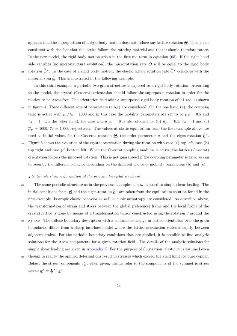
πη = −∂ψ∂η

+ πneqη , (35)

×σ =

×σ eq +

×σ neq , (36)

with the non-dissipative, non-symmetric stress given by

σ˜eq =∂ψ

∂e˜e . (37)

Note that the dissipative contribution of the stress is limited to its skew-symmetric part, for reasons

that will be explained in the next section where specific explicit constitutive laws are presented. For the

microstress ξη

and the couple stress m˜ such dissipative effects are neglected and the constitutive relations

are given by the following state laws:

ξη

=∂ψ

∂∇η, (38)

m˜ =∂ψ

∂κ˜ . (39)

The thermodynamic forces associated with the internal variable are called

Rα =∂ψ

∂rα. (40)

The remaining part of the dissipation inequality can now be written as

−πneqη η + 2×σ neq · [ ×ω e − Θ ] + 2

×σ eq · ×e ? + σ˜ : e˜p +−Rαrα ≥ 0 . (41)

where the result in equation (15) was used. In the absence of displacements the format above corresponds

to the format found by (Abrivard et al., 2012a) for the KWC model. Note that the non-equilibrium

contribution to the stress is only associated with the skew-symmetric part of the deformation.220

2.4. Evolution equations

For the dissipative contributions, a dissipation potential is introduced and decomposed in five parts

Ω = Ωθ(×σ neq) +Ω?(

×σ eq) +Ωp(σ˜p) +Ωα(Rα) +Ωη(πneqη ) , (42)

such that

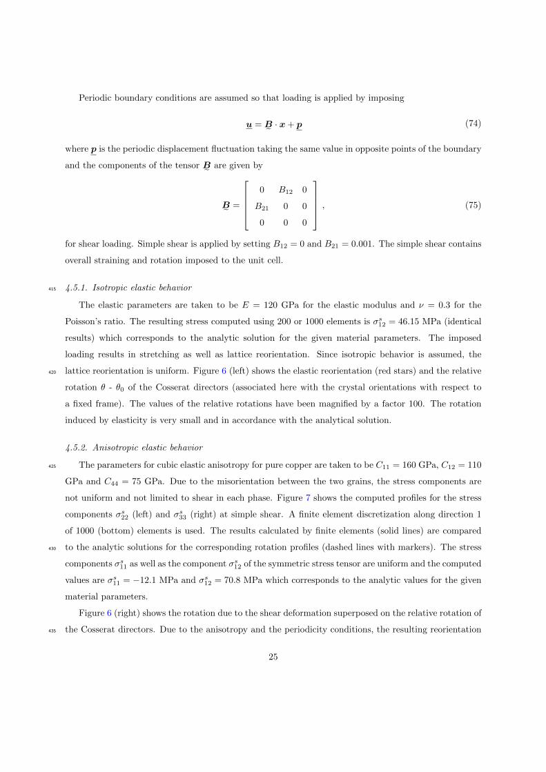
×ω e − Θ =

∂Ωθ

∂×σ neq

,×e ? =

∂Ω?

∂×σ eq

, e˜p =∂Ωp

∂σ˜ , rα = −∂Ωα

∂Rα, η = − ∂Ωη

∂πneqη. (43)

12

The skew-symmetric viscous and elastic parts of the stress tensor are therefore taken as the driving forces

for the evolution of the difference between lattice and Cosserat rotation and for the eigen-rotation, respec-

tively. These quantities are conjugate in the dissipation rate inequality (41). The plastic flow rule and

evolution laws for internal variables are also derived from the dissipation potential, as in standard gener-

alized materials (Germain et al., 1983; Maugin, 1992; Besson et al., 2009). Inserted into the dissipation

equation (41), this gives

πneqη

∂Ωη

∂πneqη+ 2

×σ neq · ∂Ωθ

∂×σ neq

+ 2×σ eq · ∂Ω

?

∂×σ eq

+ σ˜ :∂Ωp

∂σ˜ +m˜ :∂Ωp

∂m˜ +Rα∂Ω

∂Rα≥ 0 . (44)

The positivity of the dissipation rate for any process is ensured by suitable convexity properties of the

dissipation potential Ω with respect to its arguments.

3. Free energy and dissipation potentials

In order to close the system of equations it is necessary to choose specific forms of the free energy225

function ψ and of the dissipation potential Ω. A general anisotropic setting is first proposed and then

specialized to the isotropic case in order to recover the KWC equations and highlight their coupling with

mechanical contributions.

3.1. General anisotropic behavior

A general form of the free energy function which incorporates the phase field variables and the defor-

mation measures is proposed:

ψ(η,∇η, e˜e,κ˜, rα) = f0

[f(η) +

1

2∇η ·A˜ · ∇η + s g(η)||κ˜||+ ε2

2κ˜ : H

≈(η) : κ˜

]+

1

2e˜e : E

≈(η) : e˜e + ψρ(η, r

α) .

(45)

Simple quadratic contributions are chosen for the gradient phase field as usual in phase field models, and230

for Cosserat elasticity via the fourth rank tensors H≈

and E≈

. The latter are generally anisotropic. They

display major symmetry but not minor symmetry due to the non-symmetric nature of the deformation

and curvature tensors e˜e and κ˜. They may depend on the order parameter in order to distinguish

the behavior in the bulk of the grain from that in the grain boundary. The second order tensor A˜ is

symmetric. The normalization parameter f0 is taken with unit [Pa] or [J/m3] while A˜ , s and ε all have235

unit [m], leaving H≈

dimensionless. The term involving the norm of the elastic curvature tensor comes

in addition to the quadratic contribution. It is inspired by the curvature vector in the KWC model

and from potentials involving the dislocation density tensor proposed in (Conti and Ortiz, 2005; Ohno

13

and Okumura, 2007; Forest and Gueninchault, 2013; Wulfinghoff et al., 2015). The lattice curvature

tensor is often used as an approximation of the full dislocation density tensor following (Nye, 1953). The240

term ψρ(η, rα) contains the contribution due to N internal variables rα which will be associated with

dislocation density based hardening.

The resulting state laws for the generalized stresses are given by

σ˜eq =E≈

: e˜e , (46)

m˜ = f0

[s g(η)

κ˜||κ˜|| + ε2H≈

(η) : κ˜], (47)

πη = − f0

[f,η + s g,η||κ˜||+ ε2

2κ˜ : H

≈ ,η : κ˜]− 1

2e˜e : E

≈ ,η : e˜e − ψρ,η + πneqη , (48)

ξη

= f0A˜ · ∇η . (49)

where the possible dependence on η of all elastic moduli has been taken into account, the notation ,η

standing for partial derivation w.r.t. η.

Quadratic dissipation potentials Ωθ and Ωp are chosen. They ensure the positivity of the corresponding

contributions in the dissipation inequality. Such simple forms are appropriate for the description of the

relaxation phenomena in grain boundaries:

Ωθ =1

2

×σ neq · τ˜−1

θ· ×σ neq , (50)

Ω? =1

2

×σ eq · τ˜ −1

? ·×σ eq , (51)

where τ˜θ and τ˜? are constitutive symmetric positive definite, thus invertible, second order tensors.

These material parameters govern the dissipation, they are associated with the mobility of the grain

boundaries in the phase field model and have unit [Pa·s]. They may depend in general on the full set

of state variables η,∇η,κ˜, T. The equation for the dissipative stress and the evolution law for the

eigendeformation, respectively, then become

×σ neq = τ˜θ · [ ×ω e − Θ ] , (52)

×σ eq = τ˜? · ×e ? . (53)

These constitutive equations therefore are viscosity laws for the skew-symmetric parts of the stress tensors.

Equation (52) is used to compute the viscous stress from the relative rotation rate, whereas (53) is the

evolution law for the eigen-rotation in the form of a relaxation equation driven by the reversible part of

the stress.

The evolution of the crystal order parameter is likewise provided by a quadratic potential:

Ωη = τ−1η π2

η (54)

14

in the form of the usual phase field relaxation equation as in (Gurtin, 1996; Kobayashi et al., 2000;

Abrivard et al., 2012a):

−πneqη = τη η , (55)

where τη(η,∇η,κ˜, T ) is a positive scalar function. From inspection of (44) it is apparent that the formats

(52), (53) and (55) lead to non-negative contributions to the energy dissipation.

3.2. Isotropic grain boundary behavior245

The model equations can be simplified by specialization to the case of isotropic grain boundary

behavior and a separation between symmetric and skew-symmetric contributions to the deformation.

The free energy is then given by

ψ(η,∇η, e˜e,κ˜, rα) = f0

[f(η) +

a2

2|∇η|2 + s g(η)||κ˜||+ ε2

2h(η)||κ˜||2

]+

1

2ε˜e : E

≈

s : ε˜e + 2µc(η)×e e · ×e e + ψρ(η, r

α) .

(56)

The term inside brackets is essentially the same1 as introduced by (Kobayashi et al., 2000; Warren et al.,

2003). The elasticity tensor E≈

s now has both major and minor symmetry and coincides with the classical

Hooke tensor. It may be anisotropic whereas the skew-symmetric contribution is taken to be isotropic.

The Cosserat elastic modulus µc is called the coupling modulus (Lakes, 1985; Neff, 2006). It plays an

essential role in Cosserat mechanics since it relates the relative rotation to the skew-symmetric part of

the stress tensor. It acts as a penalty term limited the magnitude of the relative rotation. In the present

model, it may depend on the phase field η and thus take different values in the grain boundary and in

the bulk. The resulting state laws are given by

πη = − ∂ψ

∂η+ πneqη = −f0

[f,η + s g,η||κ˜||+ ε2

2h,η||κ˜||2

]− 2µc,η

×e e · ×e e − ψρ,η + πneqη , (57)

σ˜eq =∂ψ

∂e˜e = E≈

s : ε˜e − 2µc(η)ε˜ · ×e e , (58)

ξη

=∂ψ

∂∇η= f0 a

2∇η , (59)

m˜ =∂ψ

∂κ˜ = f0

[s g(η)

κ˜||κ˜|| + ε2 h(η)κ˜]. (60)

The skew stress pseudo-vector is given by

×σ = 2µc(η)

×e e +

×σ neq . (61)

1The only differences lie in the 3D formulation instead of the 2D KWC model and in the use of the elastic part of the

curvature tensor instead of the full curvature tensor.

15

The isotropic forms of equations (52,53) are

×σ neq = τθ [

×ω e − Θ ] , (62)

×σ eq = τ?

×e ? . (63)

Inserting the above results into the balance laws for ξη

and m˜ (while assuming all external body forces

and couples are zero) provides the evolution and partial differential equations for the phase field η and

the relative rotation in the form

τη η = f0 a2∆η − f0

[f,η + s g,η||κ˜||+ ε2

2h,η||κ˜||2

]−2µc,η

×e e · ×e e − ψρ,η , (64)

− τθ · [×ω e − Θ ] =

f0

2

[s g(η)

κ˜||κ˜|| + ε2 h(η)κ˜]· ∇+ 2µc(η)

×e e . (65)

The fundamentally new terms compared to the KWC and Abrivard models are highlighted in red. They

correspond to the contributions ensuring full coupling between phase field and mechanics. In the case of

µc(η) = 0, the format of the evolution equations closely resembles the model by Kobayashi et al. (2000);

Warren et al. (2003) with the additional stored energy term introduced by Abrivard et al. (2012a).

In the present work the Cosserat pseudo-vector Θ is interpreted as the rotation of the lattice vectors250

with respect to a fixed reference. Typically, Θ might be associated with the lattice orientations of the

grains in a polycrystal with respect to the laboratory frame. It follows that Θ 6= 0 in general even in

the otherwise undeformed configuration, i.e. with u = 0. This highlights the need for introducing the

eigen-rotation×e ?. When u = 0, the skew-symmetric deformation is given by

×e e = −Θ − ×e ?, according

to Eq. (15). The choice of initial values×e ? = −Θ ensures that the skew-symmetric equilibrium stress255

of equation (58) vanishes. Without the introduction of×e ?, it would not be possible to have a stress-free

state where u = 0 at the same time as Θ 6= 0. The introduction of the eigen-rotation can therefore be

seen as the introduction of a stress-free reference orientation of the grain. This reference evolves according

to Eq. (63) during grain boundary migration.

In the original KWC model, the evolution law for the orientation is given by the terms not marked

with red in equation (65). This format allows for the orientation inside a grain, even far from the grain

boundary, to evolve through rotation (Kobayashi et al., 2000). In order to prevent this rotation it is

necessary to distinguish between the mobility in the grain boundary and in the bulk of the grain. In

(Warren et al., 2003), this was done by considering a mobility function of the form

τθ(η,∇η,∇θ) =1

2P (||κ˜||) τθ η2 , (66)

where τθ is a constant and the mobility function P (||κ˜||) takes a high value for vanishing lattice curvature260

and a low value in the grain boundaries where the lattice curvature is pronounced. In the coupled model it

16

is expected that these rotations can instead be controlled by the Cosserat coupling term and the penalty

parameter µc(η). This will be subject of the section 4.3.

3.3. Crystal plasticity

In a crystal, plastic deformation takes place by slip on preferred directions given by N discrete slip

systems. The driving force for the activation of slip on the crystallographic slip system number α is the

resolved shear stress τα calculated as

τα = `α · σ˜ · nα (67)

where `α and nα are, respectively, the slip direction and normal to the slip plane. The kinematics of

plastic flow is governed by

e˜p =

N∑α=1

γα `α ⊗ nα . (68)

The slip rate γα is calculated according to a viscoplastic flow rule taken from Cailletaud (1992):

γα =

⟨|τα| −Rα

Kv

⟩nsign τα (69)

where 〈•〉 = Max(•, 0). The critical resolved shear stress for slip system α is Rα and Kv and n are265

viscosity parameters, with n being the Norton power law exponent.

An essential driving force for grain boundary migration is the energy stored due dislocation accu-

mulation. The dislocation part of the free energy density function in equation (45) is now taken as

ψρ(η, rα) = η

N∑α=1

λ

2µrα2 , (70)

where λ is a parameter close to 0.3 (Hirth and Lothe, 1982) and µ is the shear modulus. The internal

variables rα are now related to the stored dislocation densities ρα in the following way:

Rα =∂ψ

∂rα= ληµrα = ληµb

√√√√ N∑β=1

hαβρβ (71)

where b is the norm of the Burgers vector of the considered slip system family. The relation (71) defines

the internal variable rα as a function of the dislocation densities. The interaction between the dislocations

of the various slip systems is represented by the interaction matrix hαβ . The energy term is multiplied

by the order parameter η because the formula for stored energy by dislocation accumulation is valid in

the bulk crystal but loses its meaning inside the grain boundary. During plastic deformation, dislocations

17

are subjected to multiplication and annihilation mechanisms recorded by the following Kocks-Mecking-

Teodosiu evolution equation:

ρα =

1b

(K√∑

β ρβtot − 2dρα

)|γα|−ρα CD A(||κ˜||) η if η > 0

1b

(K√∑

β ρβtot − 2dρα

)|γα| if η ≤ 0

(72)

The evolution equation contains the term highlighted in red which is added to account for the annihilation

of dislocations behind a sweeping grain boundary. The other terms are, respectively, for the competing

dislocation storage and dynamic recovery taking place during the deformation process. The parameter K

is a mobility constant and d is the critical annihilation distance between opposite sign dislocations whereas270

the parameter CD determines the dynamics of the static recovery due to a migrating grain boundary. A

lower value means only partial recovery whereas a higher value leads to full recovery, see (Humphreys

and Hatherly, 2004) for TEM images of such static recovery processes. The function A(||κ˜||) serves to

localize the process in a thin region of the grain boundary domain. In order to ensure that recovery only

takes place in the wake of the sweeping grain boundary, not in front of it, the corresponding term is275

active only if η > 0. Such a static recovery term coupled with the crystallinity phase field was proposed

by Abrivard et al. (2012a) in the evolution equation for the total stored dislocation energy. As a further

refinement, the static recovery is written here at the level of each individual slip system.

In the present paper, the decomposition of the curvature tensor into elastic and plastic parts or of the

couple stress tensor into equilibrium and non-equilibrium parts was not considered for simplicity. The280

lattice curvature is therefore synonymous of energy storage. The reader is referred to (Forest et al., 1997;

Fleck and Hutchinson, 1997; Forest et al., 2000; Mayeur et al., 2011; Mayeur and McDowell, 2015) for

the consideration of a dissipative contribution of lattice curvature.

4. Application to lattice rotation and grain boundary migration in a laminate microstruc-

ture285

In this section results from finite element simulations of several test examples are presented and

discussed. The general geometry used for the calculations is that shown in figure 1. It is two-dimensional

and represents a laminated crystal with periodically replicated bicrystal layers, where each layer is 10 µm

wide.

The system of equations for isotropic grain boundaries reduced to two dimensions under plane strain290

conditions is detailed in Appendix A. Model parameters for pure copper are given in Appendix B along

with guidelines on their calibration. The simulations are done on a dimensionless system of characteristic

18

length Λ and time τ0, such that x = x/Λ and t = t/τ0, according to Appendix B. The free energy in

(56) is non-dimensionalized by the parameter f0. All model parameters are given in table B.1 unless

otherwise indicated. In the simulations, a 15 degree misorientation over the grain boundary is applied.295

The parameter f0 in the free energy has been calibrated so that a GB at 15 degree misorientation has an

energy of 0.5 J/m2.

4.1. Finite element implementation

The proposed phase field Cosserat theory with the constitutive equations summarized in Appendix A

has been implemented in the finite element code Z–set (Z–set package, 2013). It is based on a variational300

formulation derived from the virtual power form of the balance equations presented in Section 2.2, as

initially proposed by Ammar et al. (2009). The detailed formulation is not presented here for the sake of

brevity. The essential features of the implementation combine elements given in Forest et al. (2000) for

Cosserat crystal plasticity and in Abrivard et al. (2012a) for the KWC model. In the two-dimensional

case, the monolithic weak formulation involves 4 nodal degrees of freedom: 2 components of displacement,305

Cosserat microrotation component θ3 and phase field η. Quadratic elements with reduced integration are

used. An implicit iterative resolution scheme is used to solve the balance equations based on the Newton-

Raphson algorithm. A fourth order Runge-Kutta method with automatic time-stepping is applied to

solve the differential equations driving the internal variables of the model.

The global orthogonal coordinate system (x1, x2, x3) is given in figure 1, where direction 1 is along310

the thickness of the bicrystal layers and direction 2 is along the height. Due to periodicity, the system

is invariant along direction 2 so that only one finite element is used in that direction. The discretization

along 1 is specified in each case. A specific feature of the model is that the Cosserat rotation is used to

transform tensors between the global coordinate frame and the local frame of the crystal. The Cosserat

pseudo-vectorΘ is associated with the lattice orientations with respect to a fixed reference frame, which is315

here taken to be (x1, x2, x3). With the calculations restricted to the (x1, x2)-plane, the axis of rotation is

the x3-axis. This gives Θ = [ 0 0 θ3 ]T with θ3 the angle of rotation used to construct the appropriate

orthogonal transformation tensors between the global and the local frame. This is different from a model

using a sharp interface description since Θ in the present model varies as a phase-field variable over grain

boundaries, i.e. it is continuous everywhere in the computational domain. In what follows, the subscript320

will be dropped when referring to the rotation angle so that θ = θ3.

4.2. Grain boundary equilibrium profiles

Prior to any microstructure evolution calculation, the field variables of the model must be determined

for the initial static equilibrium state of the grain boundaries. The initial crystallinity and orientation

19

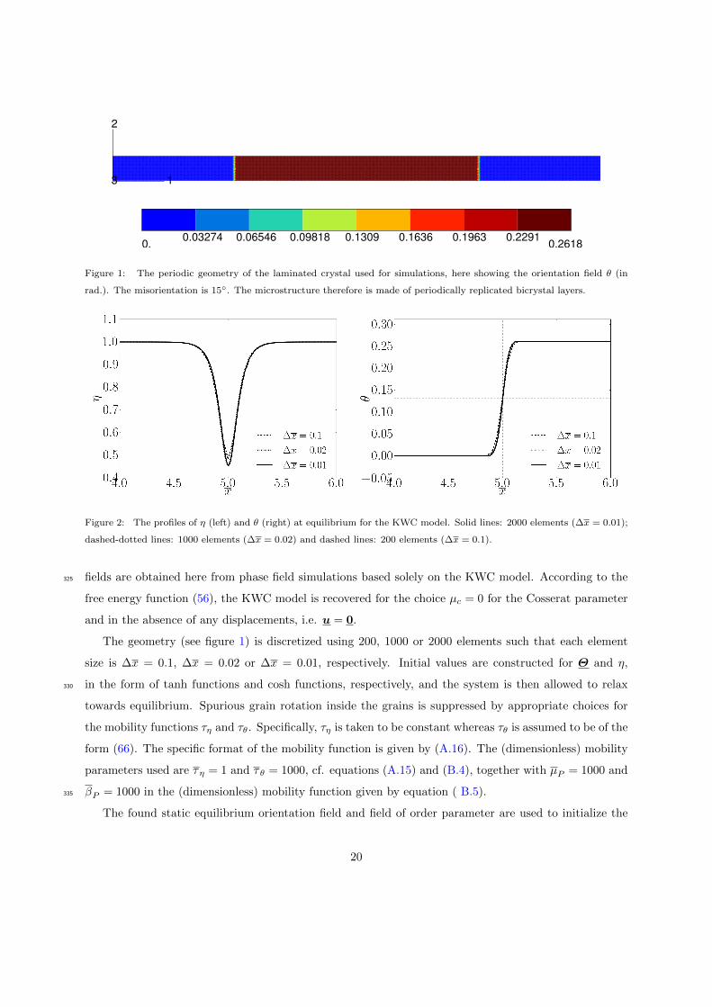
1

2

3

0. 0.26180.03274 0.06546 0.09818 0.1309 0.1636 0.1963 0.2291

Figure 1: The periodic geometry of the laminated crystal used for simulations, here showing the orientation field θ (in

rad.). The misorientation is 15. The microstructure therefore is made of periodically replicated bicrystal layers.

Figure 2: The profiles of η (left) and θ (right) at equilibrium for the KWC model. Solid lines: 2000 elements (∆x = 0.01);

dashed-dotted lines: 1000 elements (∆x = 0.02) and dashed lines: 200 elements (∆x = 0.1).

fields are obtained here from phase field simulations based solely on the KWC model. According to the325

free energy function (56), the KWC model is recovered for the choice µc = 0 for the Cosserat parameter

and in the absence of any displacements, i.e. u = 0.

The geometry (see figure 1) is discretized using 200, 1000 or 2000 elements such that each element

size is ∆x = 0.1, ∆x = 0.02 or ∆x = 0.01, respectively. Initial values are constructed for Θ and η,

in the form of tanh functions and cosh functions, respectively, and the system is then allowed to relax330

towards equilibrium. Spurious grain rotation inside the grains is suppressed by appropriate choices for

the mobility functions τη and τθ. Specifically, τη is taken to be constant whereas τθ is assumed to be of the

form (66). The specific format of the mobility function is given by (A.16). The (dimensionless) mobility

parameters used are τη = 1 and τθ = 1000, cf. equations (A.15) and (B.4), together with µP = 1000 and

βP = 1000 in the (dimensionless) mobility function given by equation ( B.5).335

The found static equilibrium orientation field and field of order parameter are used to initialize the

20

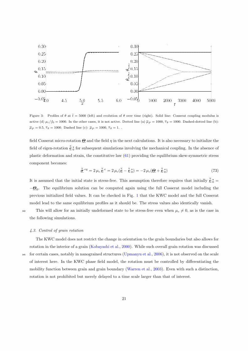
Figure 3: Profiles of θ at t = 5000 (left) and evolution of θ over time (right). Solid line: Cosserat coupling modulus is

active (d) µc/f0 = 1000. In the other cases, it is not active. Dotted line (a) µP = 1000, τθ = 1000. Dashed-dotted line (b):

µP = 0.5, τθ = 1000. Dashed line (c): µP = 1000, τθ = 1. .

field Cosserat micro-rotationΘ and the field η in the next calculations. It is also necessary to initialize the

field of eigen-rotation×e ?0 for subsequent simulations involving the mechanical coupling. In the absence of

plastic deformation and strain, the constitutive law (61) providing the equilibrium skew-symmetric stress

component becomes:×σ eq = 2µc

×e e = 2µc(

×e − ×e ?0) = −2µc(Θ +

×e ?0) (73)

It is assumed that the initial state is stress-free. This assumption therefore requires that initially×e ?0 =

−Θ0. The equilibrium solution can be computed again using the full Cosserat model including the

previous initialized field values. It can be checked in Fig. 1 that the KWC model and the full Cosserat

model lead to the same equilibrium profiles as it should be. The stress values also identically vanish.

This will allow for an initially undeformed state to be stress-free even when µc 6= 0, as is the case in340

the following simulations.

4.3. Control of grain rotation

The KWC model does not restrict the change in orientation to the grain boundaries but also allows for

rotation in the interior of a grain (Kobayashi et al., 2000). While such overall grain rotation was discussed

for certain cases, notably in nanograined structures (Upmanyu et al., 2006), it is not observed on the scale345

of interest here. In the KWC phase field model, the rotation must be controlled by differentiating the

mobility function between grain and grain boundary (Warren et al., 2003). Even with such a distinction,

rotation is not prohibited but merely delayed to a time scale larger than that of interest.

21

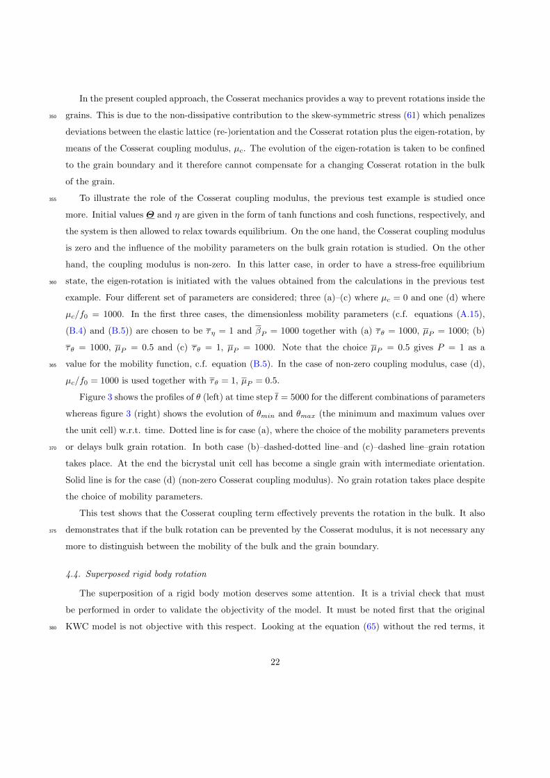
In the present coupled approach, the Cosserat mechanics provides a way to prevent rotations inside the

grains. This is due to the non-dissipative contribution to the skew-symmetric stress (61) which penalizes350

deviations between the elastic lattice (re-)orientation and the Cosserat rotation plus the eigen-rotation, by

means of the Cosserat coupling modulus, µc. The evolution of the eigen-rotation is taken to be confined

to the grain boundary and it therefore cannot compensate for a changing Cosserat rotation in the bulk

of the grain.

To illustrate the role of the Cosserat coupling modulus, the previous test example is studied once355

more. Initial values Θ and η are given in the form of tanh functions and cosh functions, respectively, and

the system is then allowed to relax towards equilibrium. On the one hand, the Cosserat coupling modulus

is zero and the influence of the mobility parameters on the bulk grain rotation is studied. On the other

hand, the coupling modulus is non-zero. In this latter case, in order to have a stress-free equilibrium

state, the eigen-rotation is initiated with the values obtained from the calculations in the previous test360

example. Four different set of parameters are considered; three (a)–(c) where µc = 0 and one (d) where

µc/f0 = 1000. In the first three cases, the dimensionless mobility parameters (c.f. equations (A.15),

(B.4) and (B.5)) are chosen to be τη = 1 and βP = 1000 together with (a) τθ = 1000, µP = 1000; (b)

τθ = 1000, µP = 0.5 and (c) τθ = 1, µP = 1000. Note that the choice µP = 0.5 gives P = 1 as a

value for the mobility function, c.f. equation (B.5). In the case of non-zero coupling modulus, case (d),365

µc/f0 = 1000 is used together with τθ = 1, µP = 0.5.

Figure 3 shows the profiles of θ (left) at time step t = 5000 for the different combinations of parameters

whereas figure 3 (right) shows the evolution of θmin and θmax (the minimum and maximum values over

the unit cell) w.r.t. time. Dotted line is for case (a), where the choice of the mobility parameters prevents

or delays bulk grain rotation. In both case (b)–dashed-dotted line–and (c)–dashed line–grain rotation370

takes place. At the end the bicrystal unit cell has become a single grain with intermediate orientation.

Solid line is for the case (d) (non-zero Cosserat coupling modulus). No grain rotation takes place despite

the choice of mobility parameters.

This test shows that the Cosserat coupling term effectively prevents the rotation in the bulk. It also

demonstrates that if the bulk rotation can be prevented by the Cosserat modulus, it is not necessary any375

more to distinguish between the mobility of the bulk and the grain boundary.

4.4. Superposed rigid body rotation

The superposition of a rigid body motion deserves some attention. It is a trivial check that must

be performed in order to validate the objectivity of the model. It must be noted first that the original

KWC model is not objective with this respect. Looking at the equation (65) without the red terms, it380

22

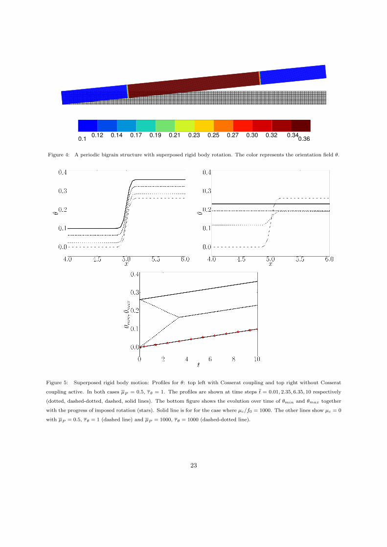
x

y

z

0.1 0.360.12 0.14 0.17 0.19 0.21 0.23 0.25 0.27 0.30 0.32 0.34

Figure 4: A periodic bigrain structure with superposed rigid body rotation. The color represents the orientation field θ.

Figure 5: Superposed rigid body motion: Profiles for θ: top left with Cosserat coupling and top right without Cosserat

coupling active. In both cases µP = 0.5, τθ = 1. The profiles are shown at time steps t = 0.01, 2.35, 6.35, 10 respectively

(dotted, dashed-dotted, dashed, solid lines). The bottom figure shows the evolution over time of θmin and θmax together

with the progress of imposed rotation (stars). Solid line is for for the case where µc/f0 = 1000. The other lines show µc = 0

with µP = 0.5, τθ = 1 (dashed line) and µP = 1000, τθ = 1000 (dashed-dotted line).

23

appears that the superposition of a rigid body motion does not induce any lattice rotation Θ. This is not

consistent with the fact that the lattice follows the rotating material and that it should therefore rotate.

In the new model, the rigid body motion arises in the first red term in equation (65). If the right hand

side vanishes (no microstructure evolution), the microrotation rate Θ will be equal to the rigid body

rotation×ω e. In the case of a rigid body motion, the elastic lattice rotation rate

×ω e coincides with the385

material spin×ω. This is illustrated in the following example.

In this third example, a periodic two-grain structure is exposed to a rigid body rotation. According

to the model, the crystal (Cosserat) orientation should follow the superposed rotation in order for the

motion to be stress free. The orientation field after a superposed rigid body rotation of 0.1 rad. is shown

in figure 4. Three different sets of parameters (a,b,c) are considered. On the one hand (a), the coupling390

term is active with µc/f0 = 1000 and in this case the mobility parameters are set to be µP = 0.5 and

τθ = 1. On the other hand, the case where µc = 0 is also studied for (b) µP = 0.5, τθ = 1 and (c)

µP = 1000, τθ = 1000, respectively. The values at static equilibrium from the first example above are

used as initial values for the Cosserat rotation Θ, the order parameter η and the eigen-rotation×e ?.

Figure 5 shows the evolution of the crystal orientation during the rotation with case (a) top left, case (b)395

top right and case (c) bottom left. When the Cosserat coupling modulus is active, the lattice (Cosserat)

orientation follows the imposed rotation. This is not guaranteed if the coupling parameter is zero, as can

be seen by the different behavior depending on the different choice of mobility parameters (b) and (c).

4.5. Simple shear deformation of the periodic bicrystal structure

The same periodic structure as in the previous examples is now exposed to simple shear loading. The400

initial conditions for η, Θ and the eigen-rotation×e ? are taken from the equilibrium solution found in the

first example. Isotropic elastic behavior as well as cubic anisotropy are considered. As described above,

the transformation of strain and stress between the global (reference) frame and the local frame of the

crystal lattice is done by means of a transformation tensor constructed using the rotation θ around the

x3-axis. The diffuse boundary description with a continuous change in lattice orientation over the grain405

boundaries differs from a sharp interface model where the lattice orientation varies abruptly between

adjacent grains. For the periodic boundary conditions that are applied, it is possible to find analytic

solutions for the stress components for a given rotation field. The details of the analytic solutions for

simple shear loading are given in Appendix C. For the purpose of illustration, elasticity is assumed even

though in reality the applied deformations result in stresses which exceed the yield limit for pure copper.410

Below, the stress components σsij , when given, always refer to the components of the symmetric stress

tensor σ˜s = E≈

s : ε˜e.24

Periodic boundary conditions are assumed so that loading is applied by imposing

u = B˜ · x+ p (74)

where p is the periodic displacement fluctuation taking the same value in opposite points of the boundary

and the components of the tensor B˜ are given by

B˜ =

0 B12 0

B21 0 0

0 0 0

, (75)

for shear loading. Simple shear is applied by setting B12 = 0 and B21 = 0.001. The simple shear contains

overall straining and rotation imposed to the unit cell.

4.5.1. Isotropic elastic behavior415

The elastic parameters are taken to be E = 120 GPa for the elastic modulus and ν = 0.3 for the

Poisson’s ratio. The resulting stress computed using 200 or 1000 elements is σs12 = 46.15 MPa (identical

results) which corresponds to the analytic solution for the given material parameters. The imposed

loading results in stretching as well as lattice reorientation. Since isotropic behavior is assumed, the

lattice reorientation is uniform. Figure 6 (left) shows the elastic reorientation (red stars) and the relative420

rotation θ - θ0 of the Cosserat directors (associated here with the crystal orientations with respect to

a fixed frame). The values of the relative rotations have been magnified by a factor 100. The rotation

induced by elasticity is very small and in accordance with the analytical solution.

4.5.2. Anisotropic elastic behavior

The parameters for cubic elastic anisotropy for pure copper are taken to be C11 = 160 GPa, C12 = 110425

GPa and C44 = 75 GPa. Due to the misorientation between the two grains, the stress components are

not uniform and not limited to shear in each phase. Figure 7 shows the computed profiles for the stress

components σs22 (left) and σs33 (right) at simple shear. A finite element discretization along direction 1

of 1000 (bottom) elements is used. The results calculated by finite elements (solid lines) are compared

to the analytic solutions for the corresponding rotation profiles (dashed lines with markers). The stress430

components σs11 as well as the component σs12 of the symmetric stress tensor are uniform and the computed

values are σs11 = −12.1 MPa and σs12 = 70.8 MPa which corresponds to the analytic values for the given

material parameters.

Figure 6 (right) shows the rotation due to the shear deformation superposed on the relative rotation of

the Cosserat directors. Due to the anisotropy and the periodicity conditions, the resulting reorientation435

25

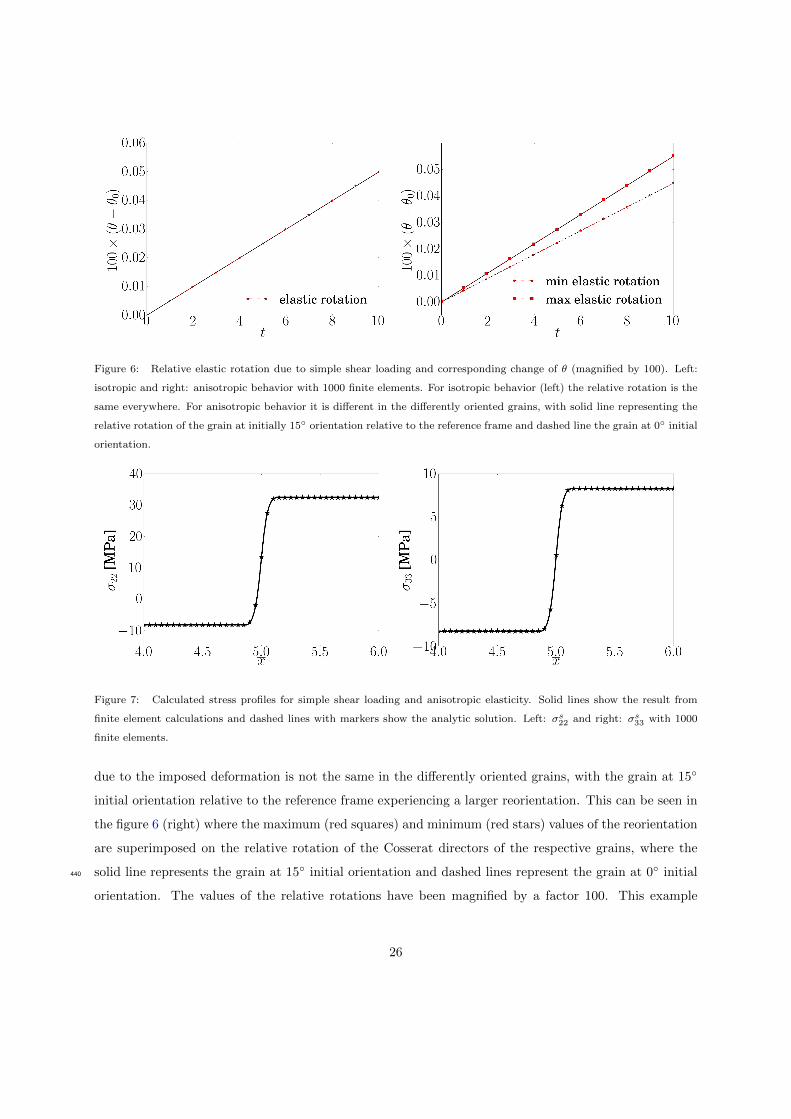
Figure 6: Relative elastic rotation due to simple shear loading and corresponding change of θ (magnified by 100). Left:

isotropic and right: anisotropic behavior with 1000 finite elements. For isotropic behavior (left) the relative rotation is the

same everywhere. For anisotropic behavior it is different in the differently oriented grains, with solid line representing the

relative rotation of the grain at initially 15 orientation relative to the reference frame and dashed line the grain at 0 initial

orientation.

Figure 7: Calculated stress profiles for simple shear loading and anisotropic elasticity. Solid lines show the result from

finite element calculations and dashed lines with markers show the analytic solution. Left: σs22 and right: σs33 with 1000

finite elements.

due to the imposed deformation is not the same in the differently oriented grains, with the grain at 15

initial orientation relative to the reference frame experiencing a larger reorientation. This can be seen in

the figure 6 (right) where the maximum (red squares) and minimum (red stars) values of the reorientation

are superimposed on the relative rotation of the Cosserat directors of the respective grains, where the

solid line represents the grain at 15 initial orientation and dashed lines represent the grain at 0 initial440

orientation. The values of the relative rotations have been magnified by a factor 100. This example

26

Figure 8: Tracking of the moving grain boundary. Top left and right shows the profiles of θ and η, respectively, at t = 0

and t = 450. Bottom left shows ρ at t = 0 and t = 450. Bottom right shows the position of the grain boundary (center)

over time, for the respective profiles.

demonstrates that the relative rotation of the Cosserat directors indeed follow the lattice reorientation

during deformation, as expected.

4.6. Grain boundary migration

A gradient in the stored energy due to plastic deformation is an important driving force for grain

boundary migration. In the proposed model, the energy due to plastic deformation is included by the

term ψρ(η, rα) in the free energy density (56). It is assumed that the stored energy is due to statistically

stored dislocations according to equations (70) and (71). Assuming for simplicity that only one slip

system is active, the energy contribution due to statistically stored dislocations becomes

ψρ(η, r) =1

2η λµ b2ρ . (76)

27

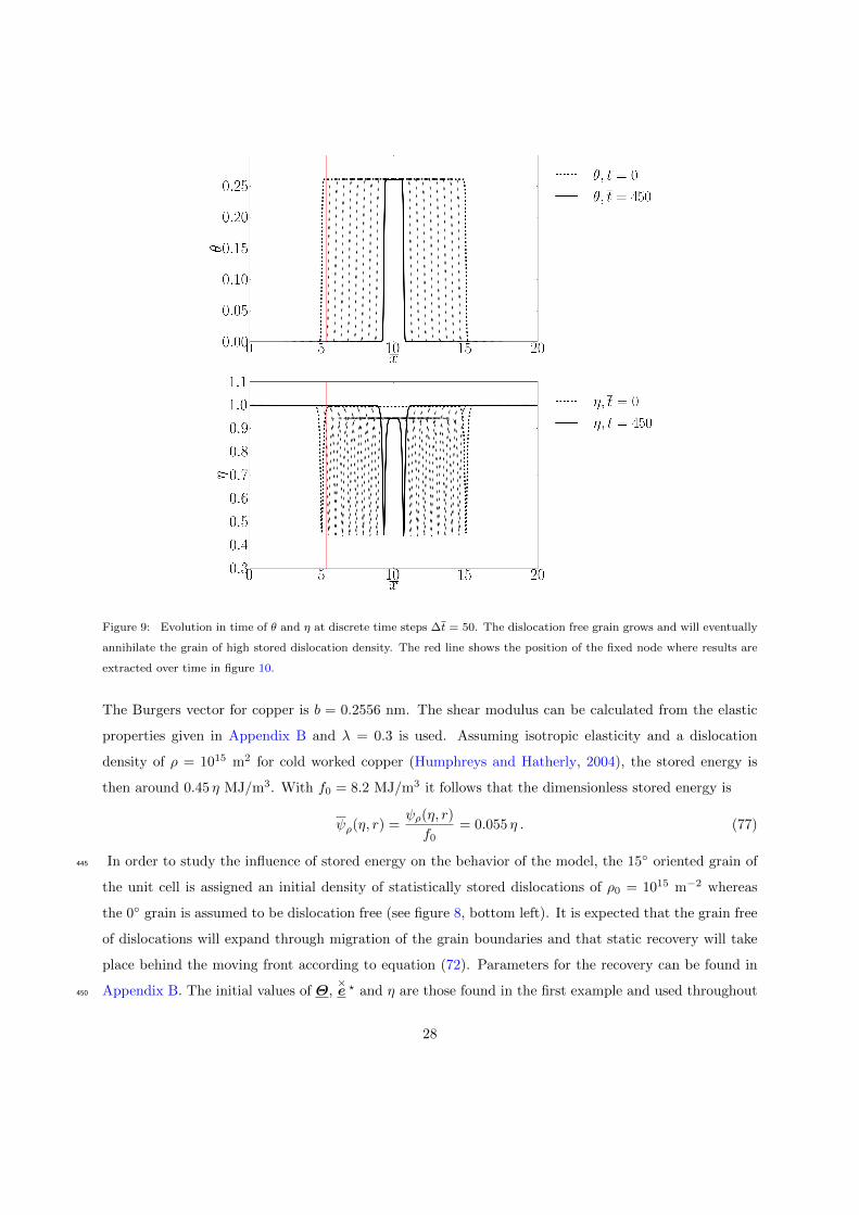
Figure 9: Evolution in time of θ and η at discrete time steps ∆t = 50. The dislocation free grain grows and will eventually

annihilate the grain of high stored dislocation density. The red line shows the position of the fixed node where results are

extracted over time in figure 10.

The Burgers vector for copper is b = 0.2556 nm. The shear modulus can be calculated from the elastic

properties given in Appendix B and λ = 0.3 is used. Assuming isotropic elasticity and a dislocation

density of ρ = 1015 m2 for cold worked copper (Humphreys and Hatherly, 2004), the stored energy is

then around 0.45 η MJ/m3. With f0 = 8.2 MJ/m3 it follows that the dimensionless stored energy is

ψρ(η, r) =ψρ(η, r)

f0= 0.055 η . (77)

In order to study the influence of stored energy on the behavior of the model, the 15 oriented grain of445

the unit cell is assigned an initial density of statistically stored dislocations of ρ0 = 1015 m−2 whereas

the 0 grain is assumed to be dislocation free (see figure 8, bottom left). It is expected that the grain free

of dislocations will expand through migration of the grain boundaries and that static recovery will take

place behind the moving front according to equation (72). Parameters for the recovery can be found in

Appendix B. The initial values of Θ,×e ? and η are those found in the first example and used throughout450

28

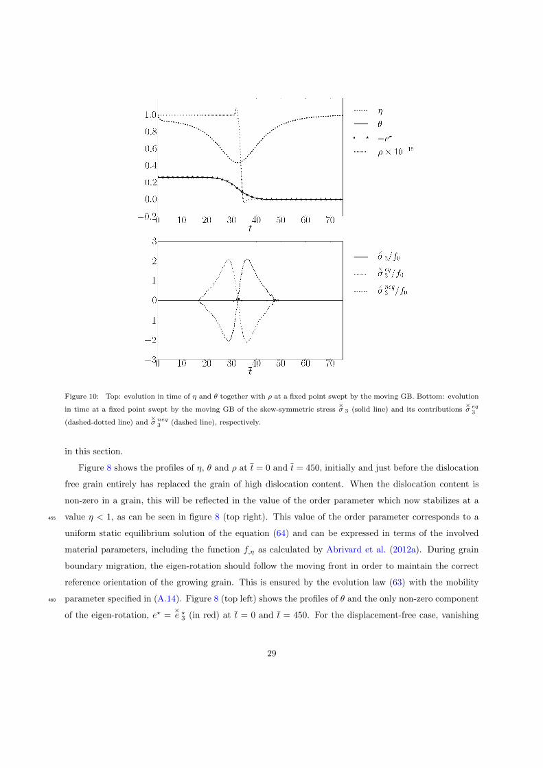
Figure 10: Top: evolution in time of η and θ together with ρ at a fixed point swept by the moving GB. Bottom: evolution

in time at a fixed point swept by the moving GB of the skew-symmetric stress×σ 3 (solid line) and its contributions

×σ eq3

(dashed-dotted line) and×σ neq3 (dashed line), respectively.

in this section.

Figure 8 shows the profiles of η, θ and ρ at t = 0 and t = 450, initially and just before the dislocation

free grain entirely has replaced the grain of high dislocation content. When the dislocation content is

non-zero in a grain, this will be reflected in the value of the order parameter which now stabilizes at a

value η < 1, as can be seen in figure 8 (top right). This value of the order parameter corresponds to a455

uniform static equilibrium solution of the equation (64) and can be expressed in terms of the involved

material parameters, including the function f,η as calculated by Abrivard et al. (2012a). During grain

boundary migration, the eigen-rotation should follow the moving front in order to maintain the correct

reference orientation of the growing grain. This is ensured by the evolution law (63) with the mobility

parameter specified in (A.14). Figure 8 (top left) shows the profiles of θ and the only non-zero component460

of the eigen-rotation, e? =×e ?3 (in red) at t = 0 and t = 450. For the displacement-free case, vanishing

29

skew-symmetric stress×σ eq requires that

×e ? = −Θ which is clearly fulfilled in this case. Furthermore, the

eigen-rotation follows the migrating grain boundary as expected, ensuring that the growing grain keeps

its stress-free reference orientation of 0. Figure 8 (bottom right) tracks the migrating grain boundary

over time for, respectively, the profile of η, θ or ρ. From the figure it is seen that the grain boundary465

velocity is constant and that the relative position of the grain boundary remains the same for all variables.

The dimensionless velocity2 of the interface is v = 9.6 · 10−3.

Figure 9 shows the profiles of θ and η over time at fixed times from t = 0 to t = 450 with ∆t = 50,

illustrating again how the dislocation free grains will grow and eventually annihilate grains of high stored

dislocation density. In figure 10 the evolution of the variables at a fixed point, swept by the moving470

interface, is represented. The point is at a distance of 0.3 µm to the right of the grain boundary inside

the 15 grain, shown by a red line in figure 9. Figure 10 (top) shows how the values of η (dashed line)

and θ (solid line) change at the node as the GB passes it. The evolution of the eigen-rotation (stars)

follows the evolution of θ. Figure 10 (top) also shows the evolution of the dislocation density at the

node (dotted line). The parameter CD in equation (72) have been chosen to be CD = 100. This value475

ensures that full static recovery takes place, as evidenced by the fact that the dislocation content is zero

when the grain boundary has passed. The static recovery becomes active at the time when η shifts from

negative to positive. Although the overall skew-symmetric stress remains zero, its components become

non-zero as the grain boundary passes the fixed point. This is shown in figure 10 (bottom) where the

solid line is the total skew-symmetric stress×σ 3 at the fixed point over time. The equilibrium contribution480

×σ eq3 to the skew-symmetric stress, which drives the evolution of the eigen-rotation in the grain boundary

according to equation (53), is shown as a dashed-dotted line. The non-equilibrium contribution×σ neq3 is

shown as dashed line. Since the total stress is zero, the equilibrium and non-equilibrium contributions

take opposite values.

5. Conclusions485

The novel features of the proposed theory are the following:

1. A general 3D anisotropic constitutive framework was proposed that intimately couples grain bound-

ary motion and mechanics. The generalization of the 2D KWC approach leads to a full 3D Cosserat

framework involving the microrotation tensor and the torsion-curvature tensor κ˜ identified as the

2If the true grain boundary velocity v at a given temperature and driving force (corresponding to the energy due to the

given dislocation content) is known then the characteristic time τ0 = t/t can be calculated as τ0 = Λv/v.

30

lattice curvature tensor. The KWC orientation field equation was interpreted as a balance equation490

for couple stresses.

2. An essential feature of the model is the concept of relative rotation representing the difference

between lattice rotation and Cosserat microrotation. This difference vanishes in the bulk of the

grain but is generally non-zero inside the grain boundary. In previous model formulations, the

rotation phase field variable and the material or lattice rotation as computed from crystal plasticity495

simulations were separate variables, whose difference was left uncontrolled.

3. An eigen-rotation variable with its relaxation equation is introduced to control the magnitude of

skew-symmetric stresses inside the grain boundaries. The skew-symmetric part of the stress tensor

in the Cosserat theory is the driving force for material reorientation inside grain boundaries. The

eigen-rotation is necessary in particular to represent stress-free initial or relaxed grain boundaries.500

The corresponding relaxation time is assumed to be much smaller than grain boundary migration

characteristic times.

4. The energetic contribution of the lattice curvature tensor has been recognized as an approximate

evaluation of the stored energy due to the dislocation density tensor. This explains the introduction

of the norm of the lattice curvature tensor in the free energy density, as initially proposed in the505

KWC model for different reasons, in addition to a quadratic contribution also used in strain gradient

plasticity (Wulfinghoff et al., 2015).

5. The model contains two contributions of dislocations to the stored energy and its evolution: stored

energy due to so-called geometrically necessary dislocations related here to the lattice curvature

tensor, and stored energy due to statistically stored dislocations described by the corresponding510

densities ρα. The Cosserat mechanics phase field contribution controls the evolution of lattice

curvature whereas an evolution law was proposed for the static recovery of stored dislocations

during grain boundary migration.

6. In the uncoupled KWC model (spurious) grain rotations had to be controlled by careful construction

of the mobility τθ. It is now naturally limited by the Cosserat coupling modulus, µc. This is a515

significant improvement of the model since the grain boundary migration rate can now be identified

independently of the overall rotation rate.

Simple examples were provided highlighting the consistency of the phase field mechanical coupling.

In the proposed theory, lattice rotation can have several origins: rigid body motion, lattice stretching

due to applied strains and grain boundary migration. The sweeping of the dislocated crystal by the grain520

boundary leads to the (possibly partial) vanishing of dislocations controlled by a static recovery term

coupled with the phase field in the dislocation density evolution equation.

31

Several features of grain boundary behavior are not accounted for in the present model: the detailed

defect structure of GB that can be found in more sophisticated models by (Berbenni et al., 2013), the

interaction between dislocations and grain boundary (dislocation absorption, annihilation, emission as525

addressed in gradient crystal plasticity contributions Wulfinghoff et al. (2013); van Beers et al. (2015)).

The next steps of the development of the model are the following. First examples of lattice rotation

induced by plastic slip and its interaction with GB migration will be explored. Comparison with recent

experimental results by Beucia et al. (2015) will be performed. The generalization to the finite deformation

and finite rotation framework will then be exposed. Finally, the anisotropic GB energy, i.e. an energy530

landscape depending on GB orientation and grain misorientation, must be incorporated explicitly by

appropriate potentials to be developed.

Acknowledgements

This project has received funding from the European Research Council (ERC) under the European

Union’s Horizon 2020 research and innovation program (grant agreement n 707392 MIGRATE).535

References

Abrivard, G., Busso, E.P., Forest, S., Appolaire, B., 2012a. Phase field modelling of grain boundary

motion driven by curvature and stored energy gradients. Part I: theory and numerical implementation.

Philosophical Magazine 92, 3618–3642.

Abrivard, G., Busso, E.P., Forest, S., Appolaire, B., 2012b. Phase field modelling of grain boundary540

motion driven by curvature and stored energy gradients. Part II: Application to recrystallisation.

Philosophical Magazine 92, 3643–3664.

Ammar, K., Appolaire, B., Cailletaud, G., Feyel, F., Forest, S., 2009. Finite element formulation of a

phase field model based on the concept of generalized stresses. Computational Materials Science 45,

800–805.545

van Beers, P., Kouznetsova, V., Geers, M., 2015. Defect redistribution within a continuum grain boundary

plasticity model. Journal of the Mechanics and Physics of Solids 83, 243 – 262. doi:http://dx.doi.

org/10.1016/j.jmps.2015.06.002.

Berbenni, S., Paliwal, B., Cherkaoui, M., 2013. A micromechanics–based model for shear–coupled grain

boundary migration in bicrystals. International Journal of Plasticity 44, 68–94.550

32

Bernacki, M., Chastel, Y., Coupez, T., Loge, R., 2008. Level set framework for the numerical modelling

of primary recrystallization in polycrystalline materials. Scripta Materialia 58, 1129–1132.

Besson, J., Cailletaud, G., Chaboche, J.L., Forest, S., Bletry, M., 2009. Non–Linear Mechanics of

Materials. Solid Mechanics and Its Applications 167, Springer-Verlag Berlin Heidelberg.

Blesgen, T., 2014. Deformation patterning in three-dimensional large-strain Cosserat plasticity. Mechanics555

Research Communications 62, 37 – 43. doi:http://dx.doi.org/10.1016/j.mechrescom.2014.08.

007.

Blesgen, T., 2017. A variational model for dynamic recrystallization based on Cosserat plasticity. Com-

posites Part B: Engineering 115, 236–243.

Beucia, B., Franciosi, P., Queyreau, S., Chaubet, D., Bacroix, B., 2015. Sem observations of grain560

boundary mobility under thermal and plasticity effects. IOP Conference Series: Materials Science and

Engineering 89, 012019. URL: http://stacks.iop.org/1757-899X/89/i=1/a=012019.

Cahn, J.W., Taylor, J.E., 2004. A unified approach to motion of grain boundaries, relative tangential

translation along grain boundaries, and grain rotation. Acta Materialia , 4887–4898.

Cailletaud, G., 1992. A micromechanical approach to inelastic behaviour of metals. International Journal565

of Plasticity 8, 55–73.

Cailletaud, G., Diard, O., Feyel, F., Forest, S., 2003. Computational crystal plasticity : From single

crystal to homogenized polycrystals. Technische Mechanik 23, 130–145.

Chen, L.Q., 1995. A novel computer simulation technique for modeling grain growth. Scripta Metallurgica

et Materialia 32, 115–120.570

Conti, S., Ortiz, M., 2005. Dislocation microstructures and the effective behavior of single crystals. Arch.

Rational Mech. Anal. 176, 103–147.

Cosserat, E., Cosserat, F., 1909. Theorie des corps deformables. Hermann, Paris.

Eringen, A.C., 1976. Polar and nonlocal field theories, in: Eringen, A.C. (Ed.), Continuum Physics. Vol

4.. Academic Press, London.575

Fan, D., Chen, L.Q., 1997. Computer simulation of grain growth using a continuum field model. Acta

Materialia 45, 611–622.

Fleck, N., Hutchinson, J., 1997. Strain gradient plasticity. Adv. Appl. Mech. 33, 295–361.

33

Forest, S., 2001–2004. Cosserat media, in: Buschow, K., Cahn, R., Flemings, M., Ilschner, B., Kramer,

E., Mahajan, S. (Eds.), Encyclopedia of Materials : Science and Technology, Elsevier. pp. 1715–1718.580

Forest, S., Barbe, F., Cailletaud, G., 2000. Cosserat modelling of size effects in the mechanical behaviour

of polycrystals and multiphase materials. International Journal of Solids and Structures 37, 7105–7126.

Forest, S., Cailletaud, G., Sievert, R., 1997. A Cosserat theory for elastoviscoplastic single crystals at

finite deformation. Archives of Mechanics 49, 705–736.

Forest, S., Gueninchault, N., 2013. Inspection of free energy functions in gradient crystal plasticity. Acta585

Mechanica Sinica 29, 763–772.

Fressengeas, c., Taupin, V., Capolungo, L., 2011. An elasto–plastic theory of dislocation and disclination

fields. International Journal of Solids and Structures 48, 3499–3509.

Germain, P., Nguyen, Q.S., Suquet, P., 1983. Continuum thermodynamics. Journal of Applied Mechanics

50, 1010–1020.590

Gottstein, G., Shvindlerman, L., 2010. Grain boundary migration in metals. CRC Press, Berlin.

Gunther, W., 1958. Zur Statik und Kinematik des Cosseratschen Kontinuums. Abhandlungen der

Braunschweig. Wiss. Ges. 10, 195–213.

Gurtin, M.E., 1996. Generalized Ginzburg-Landau and Cahn-Hilliard equations based on a microforce

balance. Physica D: Nonlinear Phenomena 92, 178–192.595

Gurtin, M.E., Lusk, M.T., 1999. Sharp-interface and phase-field theories of recrystallization in the plane.

Physica D: Nonlinear Phenomena 130, 133–154.

Guvenc, O., Bambach, M., Hirt, G., 2014. Coupling of crystal plasticity finite element and phase field

methods for the prediction of SRX kinetics after hot working. steel research international 85, 999–1009.

Guvenc, O., Henke, T., Laschet, G., Bottger, B., Apel, M., Bambach, M., Hirt, G., 2013. Modelling of600

static recrystallization kinetics by coupling crystal plasticity FEM and multiphase field calculations.

Computer Methods in Materials Science 13, 368–374.

Hirth, J., Lothe, J., 1982. Theory of Dislocations. Wiley Intersciences.

Humphreys, F., Hatherly, M., 2004. Recrystallization and Related Annealing Phenomena. Elsevier.

34

Kobayashi, R., Warren, J.A., 2005. Extending phase field models of grain boundaries to three dimensions.605

TMS Letters ArXiv:cond-mat/0502398v1 [cond-mat.mtrl-sci].

Kobayashi, R., Warren, J.A., Carter, W.C., 2000. A continuum model of grain boundaries. Physica D

140, 141–150.

Kroner, E., 1963. On the physical reality of torque stresses in continuum mechanics. Int. J. Engng. Sci.

1, 261–278.610

Kroner, E., 2001. Benefits and shortcomings of the continuous theory of dislocations. International

Journal of Solids and Structures 38, 1115–1134.

Lakes, R., 1985. A pathological situation in micropolar elasticity. J. Appl. Mech 52, 234–235. doi:10.

1115/1.3169009.

Lobkovsky, A.E., Warren, J.A., 2001. Sharp interface limit of a phase-field model of crystal grains.615

Physical Review E 63, 051605.

Mandel, J., 1973. Equations constitutives et directeurs dans les milieux plastiques et viscoplastiques. Int.

J. Solids Structures 9, 725–740.

Maugin, G.A., 1992. Thermomechanics of plasticity and fracture. Cambridge University Press.

Mayeur, J., McDowell, D., 2013. An evaluation of higher-order single crystal strength models for con-620

strained thin films subjected to simple shear. Journal of the Mechanics and Physics of Solids 61,

1935–1954. doi:http://dx.doi.org/10.1016/j.jmps.2013.04.007.

Mayeur, J., McDowell, D., 2014. A comparison of gurtin type and micropolar theories of generalized

single crystal plasticity. International Journal of Plasticity 57, 29–51. doi:http://dx.doi.org/10.

1016/j.ijplas.2014.01.010.625

Mayeur, J., McDowell, D., Bammann, D., 2011. Dislocation–based micropolar single crystal plasticity:

Comparison of multi– and single criterion theories. Journal of the Mechanics and Physics of Solids 59,

398–422.

Mayeur, J.R., McDowell, D.L., 2015. Micropolar crystal plasticity simulation of particle strengthening.

Modelling and Simulation in Materials Science and Engineering 23, 065007.630

Neff, P., 2006. The Cosserat couple modulus for continuous solids is zero viz the linearized Cauchy-

stress tensor is symmetric. ZAMM - Journal of Applied Mathematics and Mechanics / Zeitschrift fur

Angewandte Mathematik und Mechanik 86, 892–912. doi:10.1002/zamm.200510281.

35

Nye, J., 1953. Some geometrical relations in dislocated crystals. Acta Metall. 1, 153–162.

Ohno, N., Okumura, D., 2007. Higher–order stress and grain size effects due to self–energy of geometrically635

necessary dislocations. Journal of the Mechanics and Physics of Solids 55, 1879–1898.

Pusztai, T., Bortel, G., Granasy, L., 2005. Phase field theory of polycrystalline solidification in three

dimensions. EPL (Europhysics Letters) 71, 131–137.

Roters, F., Eisenlohr, P., Hantcherli, L., Tjahjanto, D., Bieler, T., Raabe, D., 2010. Overview of con-

stitutive laws, kinematics, homogenization and multiscale methods in crystal plasticity finite-element640

modeling: Theory, experiments, applications. Acta Materialia 58, 1152–1211.

Steinbach, I., Pezzolla, F., 1999. A generalized field method for multiphase transformations using interface

fields. Physica D: Nonlinear Phenomena 134, 385–393.

Steinbach, I., Pezzolla, F., Nestler, B., Seeßelberg, M., Prieler, R., Schmitz, G.J., Rezende, J.L.L., 1996.

A phase field concept for multiphase systems. Physica D: Nonlinear Phenomena 94, 135–147.645

Sun, X., Taupin, V., Fressengeas, C., Cordier, P., 2016. Continuous description of the atomic structure

of grain boundaries using dislocation and generalized-disclination density fields. International Journal

of Plasticity 77, 75 – 89. doi:http://dx.doi.org/10.1016/j.ijplas.2015.10.003.

Sutton, A., Ballufi, R., 2007. Interfaces in crystalline solids. Oxford University Press, UK.

Svendsen, B., 2002. Continuum thermodynamic models for crystal plasticity including the effects of650

geometrically-necessary dislocations. Journal of the Mechanics and Physics of Solids 50, 1297 – 1329.

doi:http://dx.doi.org/10.1016/S0022-5096(01)00124-7.

Takaki, T., Hisakuni, Y., Hirouchi, T., Yamanaka, A., Tomita, Y., 2009. Multi-phase-field simulations

for dynamic recrystallization. Computational Materials Science 45, 881–888.

Takaki, T., Tomita, Y., 2010. Static recrystallization simulations starting from predicted deformation655

microstructure by coupling multi-phase-field method and finite element method based on crystal plas-

ticity. International Journal of Mechanical Sciences 52, 320–328. Special Issue: Advances in Modeling

and Evaluation of Materials in Honor of Professor Tomita.

Taupin, V., Capolungo, L., Fressengeas, C., Das, A., Upadhyay, M., 2013. Grain boundary modeling

using an elasto-plastic theory of dislocation and disclination. Journal of the Mechanics and Physics of660

Solids 61, 370–384.

36

Trautt, Z.T., Mishin, Y., 2012. Grain boundary migration and grain rotation studied by molecular

dynamics. Acta Materialia , 2407–2424.

Tschopp, M.A., Coleman, S.P., McDowell, D.L., 2015. Symmetric and asymmetric tilt grain boundary

structure and energy in cu and al (and transferability to other fcc metals). Integrating Materials and665

Manufacturing Innovation 4, 11.

Tucker, G., McDowell, D., 2011. Non-equilibrium grain boundary structure and inelastic deformation

using atomistic simulations. International Journal of Plasticity 27, 841–857.

Upadhyay, M., Capolungo, L., Taupin, V., Fressengeas, C., 2012. Elastic constitutive laws for incompati-

ble crystalline media: the contributions of dislocations, disclinations and G-disclinations. Philosophical670

Magazine 93, 794–832.

Upadhyay, M., Capolungo, L., Taupin, V., Fressengeas, C., Lebensohn, R., 2016. A higher order elasto-

viscoplastic model using fast fourier transforms: Effects of lattice curvatures on mechanical response

of nanocrystalline metals. International Journal of Plasticity 83, 126 – 152. doi:http://dx.doi.org/

10.1016/j.ijplas.2016.04.007.675

Upmanyu, M., Srolovitz, D.J., Lobkovsky, A.E., Warren, J.A., Carter, W.C., 2006. Simultaneous grain

boundary migration and grain rotation. Acta Materialia , 1707–1719.

Vondrous, A., Bienger, P., Schreijag, S., Selzer, M., Schneider, D., Nestler, B., Helm, D., Monig, R.,

2015. Combined crystal plasticity and phase-field method for recrystallization in a process chain of

sheet metal production. Computational Mechanics 55, 439–452.680

Warren, J.A., Kobayashi, R., Lobkovsky, A.E., Carter, W.C., 2003. Extending phase field models of

solidification to polycrystalline materials. Acta Materialia 51, 6035–6058.

Wulfinghoff, S., Bayerschen, E., Bohlke, T., 2013. A gradient plasticity grain boundary yield theory.

International Journal of Plasticity 51, 33–46.

Wulfinghoff, S., Forest, S., Bohlke, T., 2015. Strain gradient plasticity modeling of the cyclic behavior685

of laminate microstructures. Journal of the Mechanics and Physics of Solids 79, 1–20. doi:10.1016/j.

jmps.2015.02.008.

Z–set package, 2013. Non-linear material & structure analysis suite, www.zset-software.com .

37

Appendix A. Model equations in 2D

Restricting the calculations to two dimensions and the axis of rotation to be the x3-axis gives Θ =690

[ 0 0 θ3 ]T with θ3 the angle of rotation. Since there are no out-of-plane rotations it also follows

that×ω = [ 0 0 ω21 ]T and

×e = [ 0 0

×e3 ]T . Furthermore, there is only one non-zero term in the

skew-symmetric stress×σ = [ 0 0

×σ3 ]T .

This allows for considerable simplification of the model equations. Dropping the subscripts on the

quantities above so that θ = θ3, ω = ω21,×e =

×e3 and

×σ =

×σ3, the principle of virtual power (ignoring

external loads) reduces to

p(i) = −πη η + ξη· ∇η − 2

×σθ +mθ · ∇θ + σ˜ : u⊗∇ . (A.1)

where mθ = [ m31 m32 m33 ]T contains the non-zero contributions to m˜ of equation (18). The weak

format of the governing equations (which are the starting point for the finite element implementation) is

then given by ∫ω

[ξη· ∇η − πη η

]dV =

∫∂ω

η ξη· ndS , (A.2)∫

ω

[mθ · ∇θ − 2

×σ θ]

dV =

∫∂ω

θmθ · n dS , (A.3)∫ω

[σ˜sym : ε˜+ 2

×σ ω

]dV =

∫∂ω

u · σ˜ · n dS . (A.4)

The term highlighted in red in the last equation is a coupling term due to the Cosserat formulation that

was not present in e.g. the formulation used in Abrivard et al. (2012a).695

The simple choice g(η) = h(η) = η2 is made in line with (Kobayashi et al., 2000), together with µc =

constant. For the function f(η) it is assumed to have a single minimum at η = 1 and is therefore taken

to be f(η) = 12 [ 1− η ]2. With these choices, the free energy function (56) becomes

ψ(η,∇η, e˜e,κ˜, rα) = f0

[1

2[ 1− η ]2 +

a2

2|∇η|2 + s η2 |∇θ|+ ε2

2η2 |∇θ|2

]+

1

2ε˜e : E

≈

s : ε˜e + 2µc [×e e]2 + η ψα(ρα) ,

(A.5)

where

ψα(ρα) =

N∑α=1

λ

2µrα2 . (A.6)

38

The constitutive equations are given by

ξη

= f0 a2∇η (A.7)

mθ = f0

[s η2 ∇θ|∇θ|

+ ε2 η2∇θ]

(A.8)

πη = − f0

[−[ 1− η ] + 2 s η |∇θ|+ ε2 η |∇θ|2

]− ψα(ρα) + πneqη (A.9)

×σ e = 2µc

×e e (A.10)

σ˜sym =E≈

s : ε˜e (A.11)

together with the evolution equations

πneqη = − τη η , (A.12)

×σ neq =

1

2P (∇θ) τθ η2 [ωe − θ] , (A.13)

×e ? = τ −1

? tanh(C2? |∇η|2)

×σ eq , (A.14)

where specific choices have been made for the viscosity type parameters τη(η,∇η,∇θ, T ), τθ(η,∇η,∇θ, T )

and τ?(η,∇η,∇θ, T ) which govern the evolution of the model toward equilibrium. In particular, by

allowing them to depend on η, ∇η and ∇θ it is possible to distinguish between behavior in the grain and

in the grain boundary. In general the mobility functions are strongly temperature dependent although,

for brevity, this will not be explored in this work and it will be assumed that all simulations are done at

constant temperature. Temperature dependence can easily be introduced in the formulation by e.g. an

Arrhenius type law as in Abrivard et al. (2012a). In accordance with Warren et al. (2003), it is assumed

that τη is constant and that

τθ(η,∇η,∇θ, T ) =1

2P (∇θ) τθ η2 (A.15)

with

P (∇θ) = 1−[

1− µPε

]exp(−βP ε |∇θ|) . (A.16)

The mobility function P differentiates between the behavior in the bulk, where it can be made arbitrarily

large through the choice of the parameter µP , and the behavior in the grain boundary where it approaches

P = 1 for large values of the parameter βP . This provides a means of separating the time scales for grain

boundary migration and grain rotation. It is necessary that P be dimensionless so the unit of µP is [m]

while βP has no unit. For the evolution of the eigen-rotation the viscosity type parameter is taken as

τ? = τ ? tanh−1(C2? |∇η|2) , (A.17)

where the format has been chosen so that the evolution is restricted to the grain boundary. The parameter

C? has unit [m].

39

The balance equations together with the above results now give

τη η = f0 a2∆η − f0

[−[ 1− η ] + 2 s η |∇θ|+ ε2 η |∇θ|2

]− ψα(ρα) , (A.18)

P (∇θ) τθ η2 [ωe − θ] = −∇ · f0

[s η2 ∇θ|∇θ|

+ ε2 η2∇θ]−4µc

×e e . (A.19)

The terms highlighted in red are the terms which are new compared to the model by Kobayashi et al.

(2000); Warren et al. (2003) and (Abrivard et al., 2012a).

The function A(||κ˜||) in equation (72) is chosen to be

A(|∇θ|) = tanh(C2A |∇θ|2) , (A.20)

where the parameter CA has unit [m].700

Appendix B. Model parameters

Model parameters are chosen to be in the reasonable range for a test material, in this case pure

copper, although a rigorous parameter fitting to experimental data has not been performed at this stage

of general model development. Some parameters, such as elastic constants, can easily be found from

reference literature. For the Cosserat parameter, µc, it is required that it is large enough to penalize705

differences between the rate of lattice rotation and the rate of Cosserat rotation in the bulk of the grain.

The parameters f0, a, s and ε together with the mobility parameters can be identified using the results

of Lobkovsky and Warren (2001) who analyzed the KWC model in the sharp interface limit using formal

asymptotics. They found expressions for the grain boundary energy and mobility as functions of the

model parameters and the misorientation between the grains.710

In order to non-dimensionalize the energy, a suitable length scale Λ of unit [m] is introduced to obtain

the dimensionless coordinates (x, y, z) = 1Λ (x, y, z). The dimensionless differential operator ∇ is then

given by ∇ = Λ∇. Furthermore, κ˜ = Θ ⊗∇ = Λκ˜. By division with f0, the dimensionless free energy

function is then found to be

ψ =ψ

f0= f(η) +

a2

2|∇η|2 + s g(η)|∇θ|+ ε2

2h(η)|∇θ|2

+1

2ε˜e : E

≈

s: ε˜e + 2µc(η) [

×e e]2 + η ψ

α(ρα) ,

(B.1)

where a = a/Λ, s = s/Λ and ε = ε/Λ are now dimensionless and

E≈

s=

1

f0E≈

s , µc =µcf0, ψ

α=ψα

f0. (B.2)

40

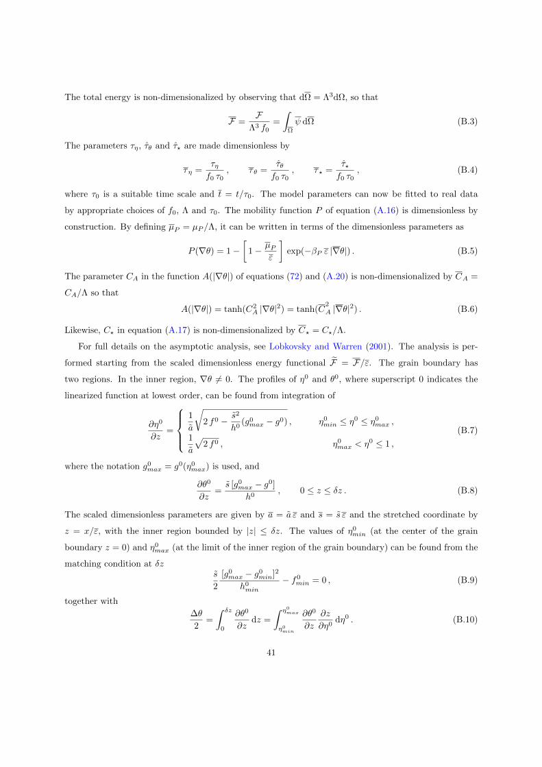
The total energy is non-dimensionalized by observing that dΩ = Λ3dΩ, so that

F =F

Λ3 f0=

∫Ω

ψ dΩ (B.3)

The parameters τη, τθ and τ? are made dimensionless by

τη =τηf0 τ0

, τθ =τθf0 τ0

, τ? =τ?f0 τ0

, (B.4)

where τ0 is a suitable time scale and t = t/τ0. The model parameters can now be fitted to real data

by appropriate choices of f0, Λ and τ0. The mobility function P of equation (A.16) is dimensionless by

construction. By defining µP = µP /Λ, it can be written in terms of the dimensionless parameters as

P (∇θ) = 1−[

1− µPε

]exp(−βP ε |∇θ|) . (B.5)

The parameter CA in the function A(|∇θ|) of equations (72) and (A.20) is non-dimensionalized by CA =

CA/Λ so that

A(|∇θ|) = tanh(C2A |∇θ|2) = tanh(C

2

A |∇θ|2) . (B.6)

Likewise, C? in equation (A.17) is non-dimensionalized by C? = C?/Λ.

For full details on the asymptotic analysis, see Lobkovsky and Warren (2001). The analysis is per-

formed starting from the scaled dimensionless energy functional F = F/ε. The grain boundary has

two regions. In the inner region, ∇θ 6= 0. The profiles of η0 and θ0, where superscript 0 indicates the

linearized function at lowest order, can be found from integration of

∂η0

∂z=

1

a

√2 f0 − s2

h0(g0max − g0) , η0

min ≤ η0 ≤ η0max ,

1

a

√2 f0 , η0

max < η0 ≤ 1 ,

(B.7)

where the notation g0max = g0(η0

max) is used, and

∂θ0

∂z=s [g0

max − g0]

h0, 0 ≤ z ≤ δz . (B.8)

The scaled dimensionless parameters are given by a = a ε and s = s ε and the stretched coordinate by

z = x/ε, with the inner region bounded by |z| ≤ δz. The values of η0min (at the center of the grain

boundary z = 0) and η0max (at the limit of the inner region of the grain boundary) can be found from the

matching condition at δzs

2

[g0max − g0

min]2

h0min

− f0min = 0 , (B.9)

together with

∆θ

2=

∫ δz

0

∂θ0

∂zdz =

∫ η0max

η0min

∂θ0

∂z

∂z

∂η0dη0 . (B.10)

41

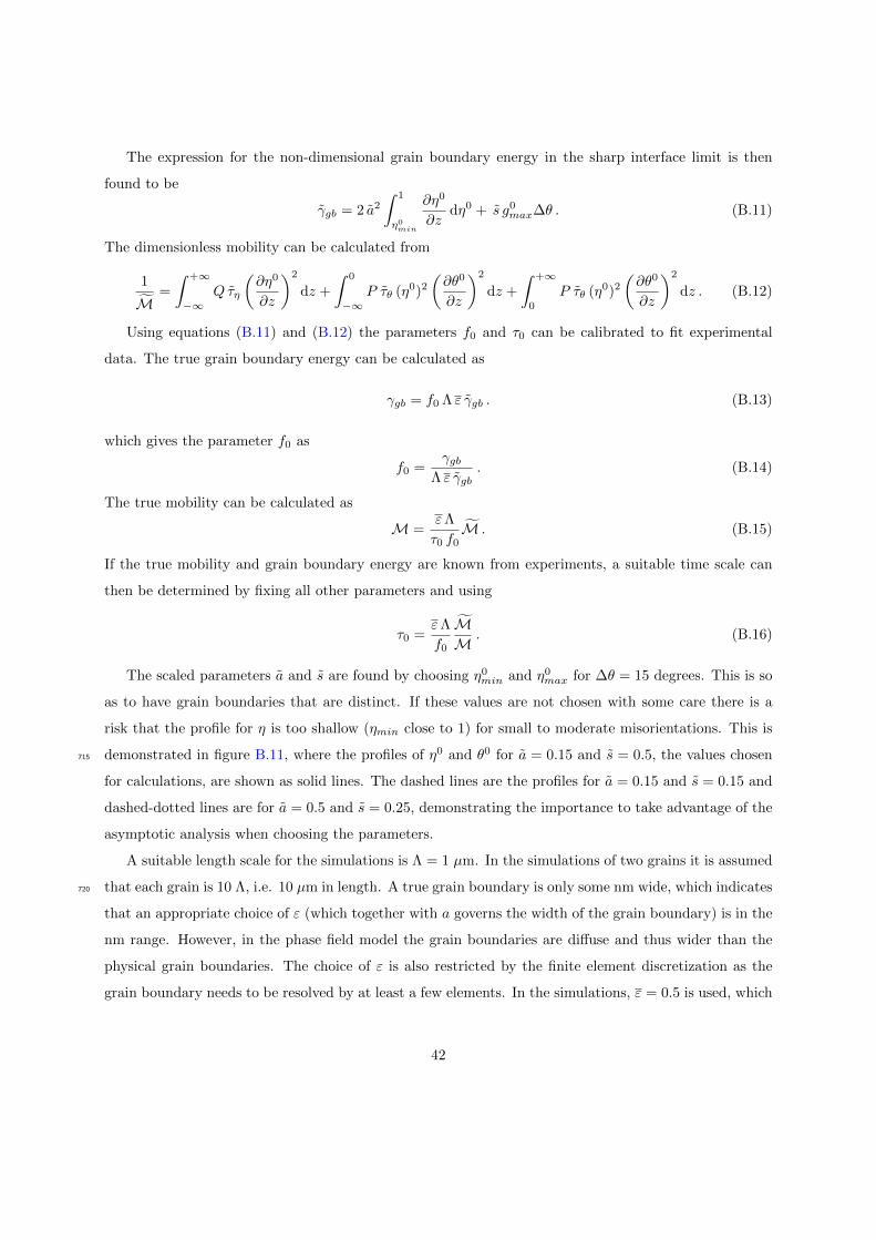
The expression for the non-dimensional grain boundary energy in the sharp interface limit is then

found to be

γgb = 2 a2

∫ 1

η0min

∂η0

∂zdη0 + s g0

max∆θ . (B.11)

The dimensionless mobility can be calculated from

1

M=

∫ +∞

−∞Q τη

(∂η0

∂z

)2

dz +

∫ 0

−∞P τθ (η0)2

(∂θ0

∂z

)2

dz +

∫ +∞

0

P τθ (η0)2

(∂θ0

∂z

)2

dz . (B.12)

Using equations (B.11) and (B.12) the parameters f0 and τ0 can be calibrated to fit experimental

data. The true grain boundary energy can be calculated as

γgb = f0 Λ ε γgb . (B.13)

which gives the parameter f0 as

f0 =γgb

Λ ε γgb. (B.14)

The true mobility can be calculated as

M =εΛ

τ0 f0M . (B.15)

If the true mobility and grain boundary energy are known from experiments, a suitable time scale can

then be determined by fixing all other parameters and using

τ0 =εΛ

f0

MM

. (B.16)

The scaled parameters a and s are found by choosing η0min and η0

max for ∆θ = 15 degrees. This is so

as to have grain boundaries that are distinct. If these values are not chosen with some care there is a

risk that the profile for η is too shallow (ηmin close to 1) for small to moderate misorientations. This is

demonstrated in figure B.11, where the profiles of η0 and θ0 for a = 0.15 and s = 0.5, the values chosen715

for calculations, are shown as solid lines. The dashed lines are the profiles for a = 0.15 and s = 0.15 and

dashed-dotted lines are for a = 0.5 and s = 0.25, demonstrating the importance to take advantage of the

asymptotic analysis when choosing the parameters.

A suitable length scale for the simulations is Λ = 1 µm. In the simulations of two grains it is assumed

that each grain is 10 Λ, i.e. 10 µm in length. A true grain boundary is only some nm wide, which indicates720

that an appropriate choice of ε (which together with a governs the width of the grain boundary) is in the

nm range. However, in the phase field model the grain boundaries are diffuse and thus wider than the

physical grain boundaries. The choice of ε is also restricted by the finite element discretization as the

grain boundary needs to be resolved by at least a few elements. In the simulations, ε = 0.5 is used, which

42

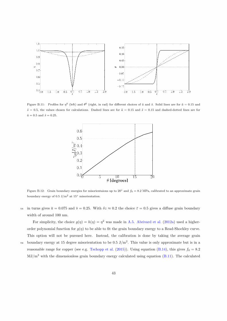
Figure B.11: Profiles for η0 (left) and θ0 (right, in rad) for different choices of a and s. Solid lines are for a = 0.15 and

s = 0.5, the values chosen for calculations. Dashed lines are for a = 0.15 and s = 0.15 and dashed-dotted lines are for

a = 0.5 and s = 0.25.

Figure B.12: Grain boundary energies for misorientaions up to 20 and f0 = 8.2 MPa, calibrated to an approximate grain

boundary energy of 0.5 J/m2 at 15 misorientation.

in turns gives a = 0.075 and s = 0.25. With δz ≈ 0.2 the choice ε = 0.5 gives a diffuse grain boundary725

width of around 100 nm.

For simplicity, the choice g(η) = h(η) = η2 was made in A.5. Abrivard et al. (2012a) used a higher-

order polynomial function for g(η) to be able to fit the grain boundary energy to a Read-Shockley curve.

This option will not be pursued here. Instead, the calibration is done by taking the average grain

boundary energy at 15 degree misorientation to be 0.5 J/m2. This value is only approximate but is in a730

reasonable range for copper (see e.g. Tschopp et al. (2015)). Using equation (B.14), this gives f0 = 8.2

MJ/m3 with the dimensionless grain boundary energy calculated using equation (B.11). The calculated

43

grain boundary energy for misorientations from 0 up to 20 is shown in figure B.12.

Name Unit Value

f0 [J/m3] = [Pa] 8.2 MPa

a [m] 0.075 µm

s [m] 0.25 µm

ε [m] 0.5 µm

CD 100

CA [m] 10 µm

C? [m] 10 µm

τη [J·s/m3] = [Pa s] 1 f0 τ0

τθ [Js/m3] = [Pa s] 1 f0 τ0

τ? [J·s/m3] = [Pa s] 0.1 f0 τ0

λ 0.3

b [m] 0.2556 nm

Cubic anisotropy

C11 [J/m3] 160 GPa

C12 [J/m3] 110 GPa

C44 [J/m3] 75 GPa

Table B.1: List of model parameters used to produce the numerical examples, unless otherwise stated.

The full set of parameters along with their units is presented in table B.1. The time scale parameter

can easily be fitted to a true mobility value using equation (B.16) together with (B.12).735

Appendix C. Analytic solution of the stresses during shear loading

Periodic boundary conditions are assumed so that loading is applied by imposing

u = B˜ · x+ p (C.1)

where p is the periodic fluctuation vector taking the same value in opposing points of the boundary and

the components of the tensor B˜ are given by

B˜ =

0 B12 0

B21 0 0

0 0 0

, (C.2)

44

for shear loading. Specifically, for simple shear with B12 = 0 and the problem at hand, the components

of the displacement vector are given by

u1 = p1(x1) ,

u2 =B21 x1 + p2(x1) ,

u3 = 0 .

(C.3)

The only non-zero strains (in the small deformation setting) are then given by

ε11 =∂u1

∂x1= p1,1 , ε12 = ε21 =

1

2

[∂u1

∂x2+∂u2

∂x1

]=

1

2[B21 + p2,1 ] , (C.4)

whereas

ε22 = 0 (C.5)

due to the imposed boundary conditions and all other strain components are zero due to the plane strain

conditions. Furthermore, the following holds

〈ε11〉 = 0 , 〈ε12〉 =1

2B21 . (C.6)

Cubic anisotropy is assumed so that the elastic stiffness tensor has three independent parameters C11,

C12 and C44. Likewise, the compliance tensor has only three independent parameters S11, S12 and S44

which can be related to the modulus of elasticity through

S11 =C11 + C12

(C11 + 2C12) (C11 − C12)S12 =

−C12

(C11 + 2C12) (C11 − C12)S44 =

1

S44. (C.7)

Strain and stress are rotated between the global frame and the local frame of the lattice through transfor-

mation matrices constructed using the non-constant rotation field parameter θ. The constitutive relation

between stress and strain is applied in the local frame. Finally, an expression for the strains in the global

frame is obtained as

ε11 =Aσ11 +B σ22 − C σ12 ,

ε22 =B σ11 +Aσ22 + C σ12 ,

ε12 = − 1

2C [ σ11 −Aσ22 ] +Dσ12 ,

ε33 =S12 [σ11 + σ22 ] + S11 σ33 ,

(C.8)

45

where the coefficients are given by

A =S11 + SD + SA sin2(2θ) ,

B =S12 + SD − SA sin2(2θ) ,

C =SA sin(4θ) ,

D =SB + SA cos(4θ) ,

SA =1

2

[−S11 + S12 +

1

2S44

],

SB =1

2

[S11 − S12 +

1

2S44

],

SD = − S212

S11,

(C.9)

and it was used that ε33 = 0 (plane strain) to express σ33 in terms of σ11 and σ22 in the equations for

ε11 and ε22.

It is now possible to construct a system of equations to solve for the stresses. First, as already noted,

due to the imposed loading (pure strain) the out-of-plane strain is zero

ε33 = S12 [σ11 + σ22 ] + S11 σ33 = 0 ⇒ σ33 = −S12

S11[σ11 + σ22 ] . (C.10)

For the stresses, the following holds for the averages

〈σ33〉 = 0 , 〈σ11〉 = σ11 , 〈σ12〉 = σ12 . (C.11)

This together with ε33 = 0 gives the first equation

〈σ33〉 = 0 ⇒ σ11 = −〈σ22〉 . (C.12)

The second equation comes from the fact that ε22 = 0, i.e.

B σ11 +Aσ22 + C σ12 = 0 , (C.13)

and the third equation comes from the condition

〈ε12〉 =1

2B21 , (C.14)

so that finally a system of equation in three unknowns σ11, σ22 and σ12 can be written asB σ11 +Aσ22 + C σ12 = 0 , (1)⟨−1

2C [ σ11 −Aσ22 ] +Dσ12

⟩=

1

2B21 , (2)

σ11 = −〈σ22〉 . (3)

(C.15)

46

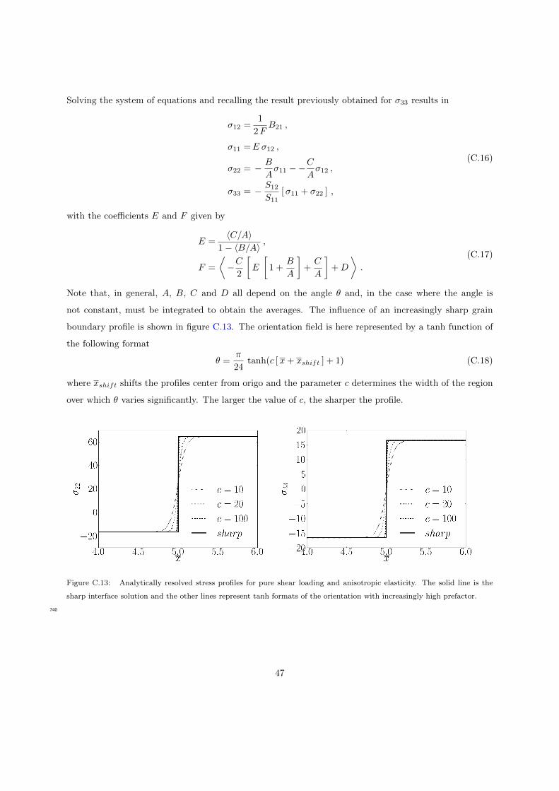
Solving the system of equations and recalling the result previously obtained for σ33 results in

σ12 =1

2FB21 ,

σ11 =E σ12 ,

σ22 = − B

Aσ11 −−

C

Aσ12 ,

σ33 = − S12

S11[σ11 + σ22 ] ,

(C.16)

with the coefficients E and F given by

E =〈C/A〉

1− 〈B/A〉,

F =

⟨−C

2

[E

[1 +

B

A

]+C

A

]+D

⟩.

(C.17)

Note that, in general, A, B, C and D all depend on the angle θ and, in the case where the angle is

not constant, must be integrated to obtain the averages. The influence of an increasingly sharp grain

boundary profile is shown in figure C.13. The orientation field is here represented by a tanh function of

the following format

θ =π

24tanh(c [x+ xshift ] + 1) (C.18)

where xshift shifts the profiles center from origo and the parameter c determines the width of the region

over which θ varies significantly. The larger the value of c, the sharper the profile.

Figure C.13: Analytically resolved stress profiles for pure shear loading and anisotropic elasticity. The solid line is the

sharp interface solution and the other lines represent tanh formats of the orientation with increasingly high prefactor.

740

47