


Languages
Pages
Legal

2010-03-15
851-0585-04L – Modelling and Simulating Social Systems with MATLAB
Lesson 4 – Cellular Automata
Anders Johansson and Wenjian Yu
© ETH Zürich |
2010-03-15 A. Johansson & W. Yu / [email protected] [email protected] 2
Lesson 4 – Contents
� Cellular Automata
� Neighborhood definitions
� Models
� Game of Life
� Highway Simulation
� Disease Spreading, revisited
� Exercises
2010-03-15 A. Johansson & W. Yu / [email protected] [email protected] 3
Cellular Automaton (plural: Automata)
� A cellular automaton is a rule, defining how the
state of a cell in a grid is updated, depending on
the states of its neighbor cells.
� They are represented as grids with arbitrary
dimension.
� Cellular-automata simulations are discrete both
in time and space.
2010-03-15 A. Johansson & W. Yu / [email protected] [email protected] 4
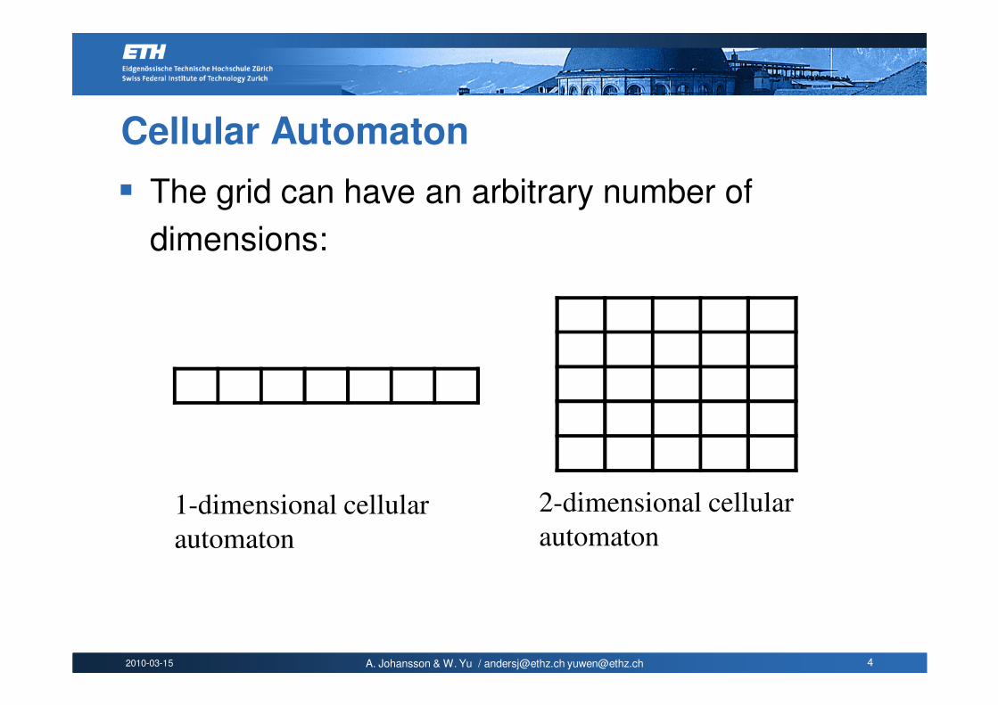
Cellular Automaton
� The grid can have an arbitrary number of
dimensions:
1-dimensional cellular
automaton
2-dimensional cellular
automaton
2010-03-15 A. Johansson & W. Yu / [email protected] [email protected] 5
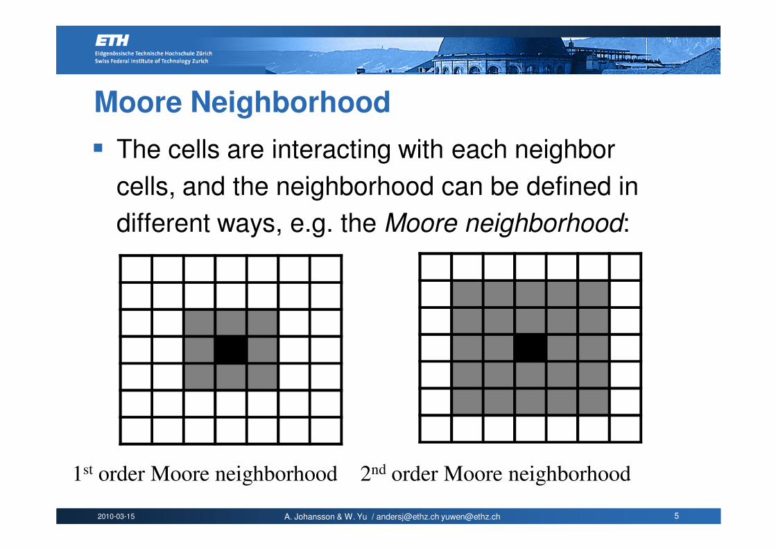
Moore Neighborhood
� The cells are interacting with each neighbor
cells, and the neighborhood can be defined in
different ways, e.g. the Moore neighborhood:
1st order Moore neighborhood 2nd order Moore neighborhood
2010-03-15 A. Johansson & W. Yu / [email protected] [email protected] 6
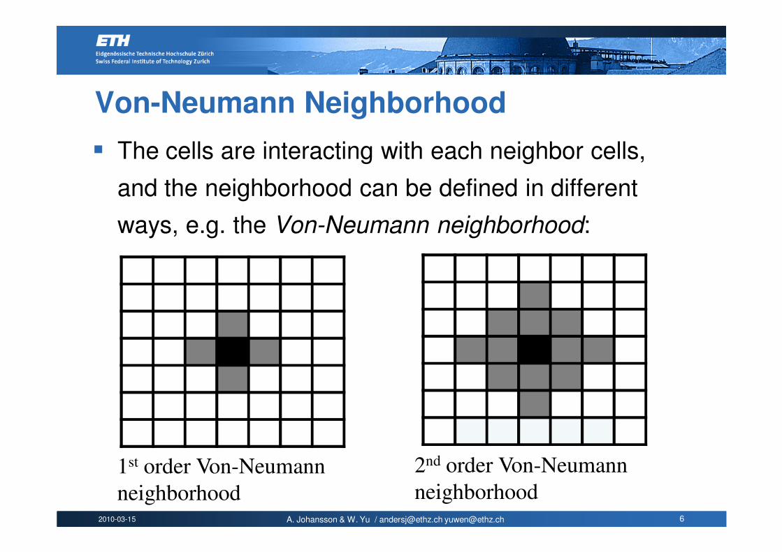
Von-Neumann Neighborhood
� The cells are interacting with each neighbor cells,
and the neighborhood can be defined in different
ways, e.g. the Von-Neumann neighborhood:
1st order Von-Neumann
neighborhood
2nd order Von-Neumann
neighborhood
2010-03-15 A. Johansson & W. Yu / [email protected] [email protected] 7
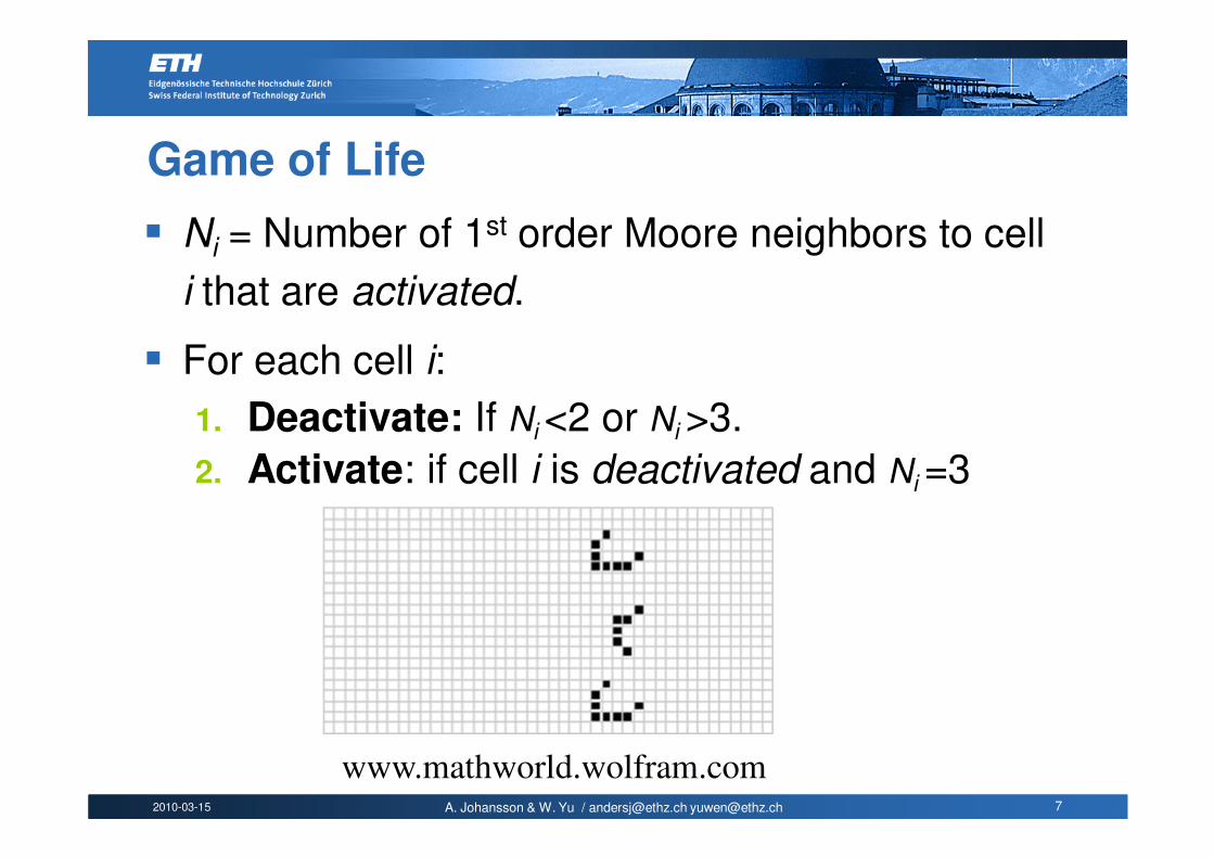
Game of Life
� Ni = Number of 1st order Moore neighbors to cell
i that are activated.
� For each cell i:
1. Deactivate: If Ni <2 or Ni >3.
2. Activate: if cell i is deactivated and Ni =3
www.mathworld.wolfram.com
2010-03-15 A. Johansson & W. Yu / [email protected] [email protected] 8
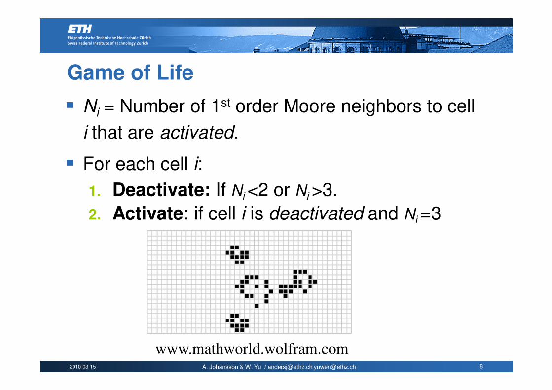
Game of Life
www.mathworld.wolfram.com
� Ni = Number of 1st order Moore neighbors to cell
i that are activated.
� For each cell i:
1. Deactivate: If Ni <2 or Ni >3.
2. Activate: if cell i is deactivated and Ni =3

2010-03-15 A. Johansson & W. Yu / [email protected] [email protected] 9
Highway Simulation
� As an example of a 1-dimensional cellular
automaton, we will present a highway
simulation. For each car at cell i:
1. Stay: If the cell directly to the right is occupied.
2. Move: Otherwise, move one step to the right, with
probability p
Move to the next cell, with
the probability p
2010-03-15 A. Johansson & W. Yu / [email protected] [email protected] 10
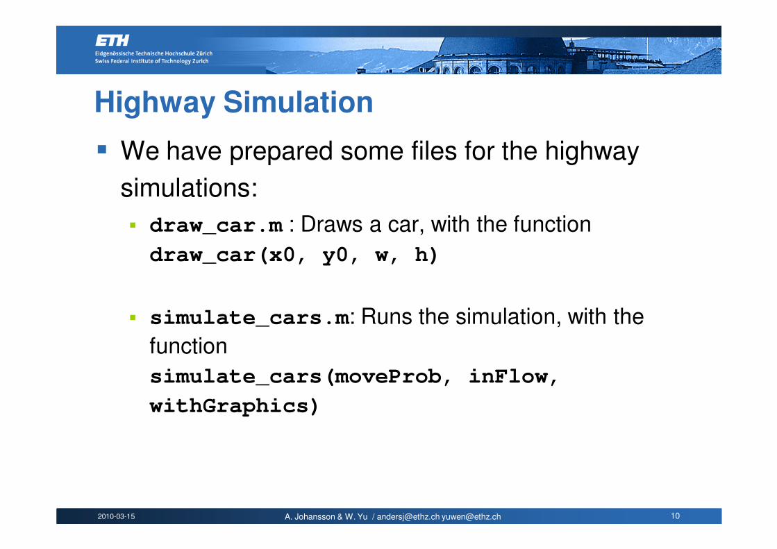
Highway Simulation
� We have prepared some files for the highway
simulations:
� draw_car.m : Draws a car, with the function
draw_car(x0, y0, w, h)
� simulate_cars.m: Runs the simulation, with the
function
simulate_cars(moveProb, inFlow,
withGraphics)
2010-03-15 A. Johansson & W. Yu / [email protected] [email protected] 11
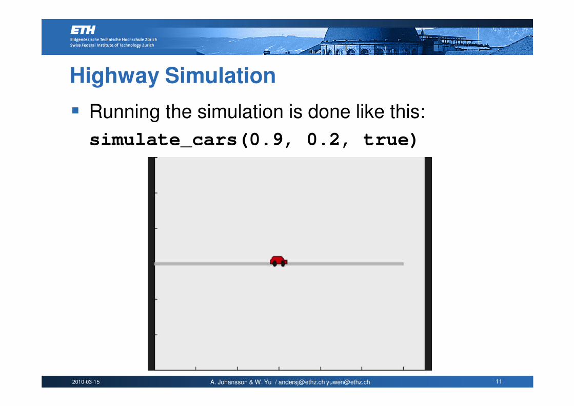
Highway Simulation
� Running the simulation is done like this:
simulate_cars(0.9, 0.2, true)
2010-03-15 A. Johansson & W. Yu / [email protected] [email protected] 12
Kermack-McKendrick Model
� In lesson 3, we introduced the Kermack-
McKendrick model, used for simulating disease
spreading.
� We will now implement the model again, but this
time within the cellular-automata framework.
2010-03-15 A. Johansson & W. Yu / [email protected] [email protected] 13
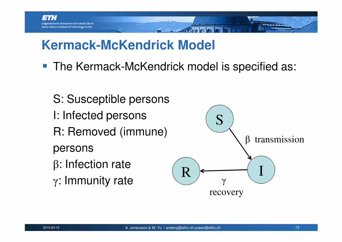
Kermack-McKendrick Model
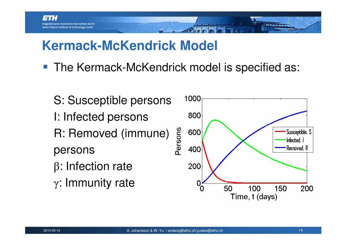
� The Kermack-McKendrick model is specified as:
S: Susceptible persons
I: Infected persons
R: Removed (immune)
persons
β: Infection rate
γ: Immunity rate
S
IR
β transmission
γ
recovery
2010-03-15 A. Johansson & W. Yu / [email protected] [email protected] 14
Kermack-McKendrick Model
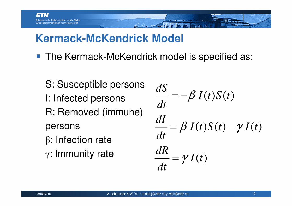
� The Kermack-McKendrick model is specified as:
S: Susceptible persons
I: Infected persons
R: Removed (immune)
persons
β: Infection rate
γ: Immunity rate
2010-03-15 A. Johansson & W. Yu / [email protected] [email protected] 15
Kermack-McKendrick Model
� The Kermack-McKendrick model is specified as:
S: Susceptible persons
I: Infected persons
R: Removed (immune)
persons
β: Infection rate
γ: Immunity rate )(
)( )()(
)()(
tIdt
dR
tItStIdt
dI
tStIdt
dS
γ
γβ
β
=
−=
−=
2010-03-15 A. Johansson & W. Yu / [email protected] [email protected] 16
Kermack-McKendrick Model
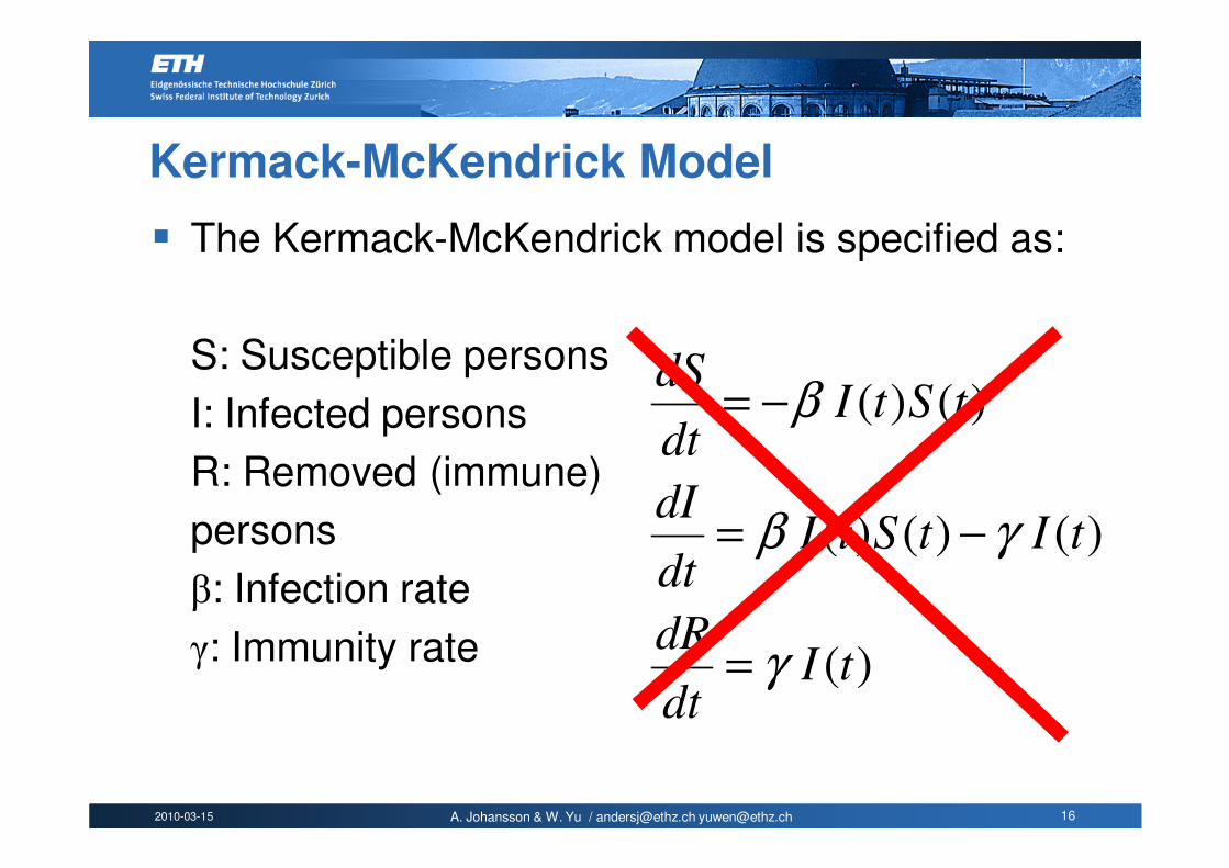
� The Kermack-McKendrick model is specified as:
S: Susceptible persons
I: Infected persons
R: Removed (immune)
persons
β: Infection rate
γ: Immunity rate )(
)( )()(
)()(
tIdt
dR
tItStIdt
dI
tStIdt
dS
γ
γβ
β
=
−=
−=
2010-03-15 A. Johansson & W. Yu / [email protected] [email protected] 17
Kermack-McKendrick Model
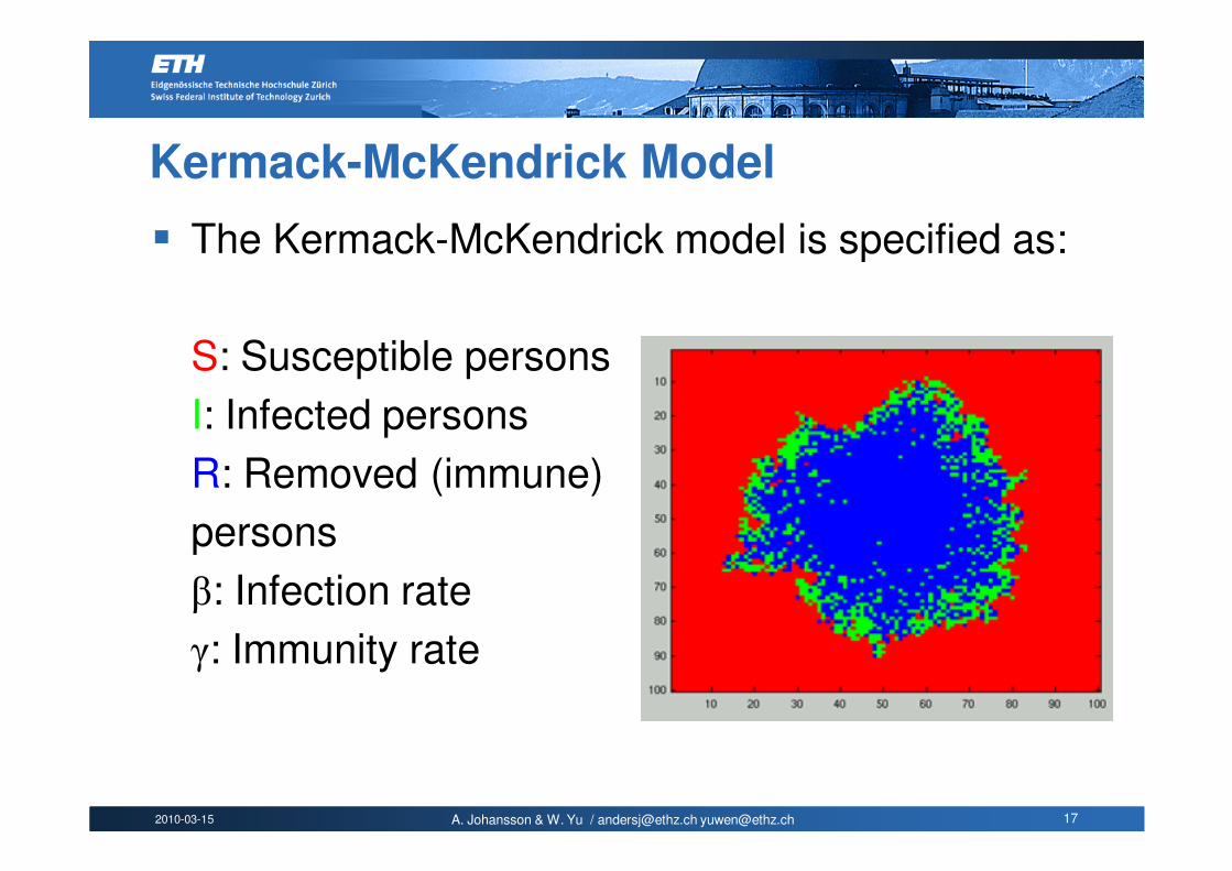
� The Kermack-McKendrick model is specified as:
S: Susceptible persons
I: Infected persons
R: Removed (immune)
persons
β: Infection rate
γ: Immunity rate
2010-03-15 A. Johansson & W. Yu / [email protected] [email protected] 18
Kermack-McKendrick Model
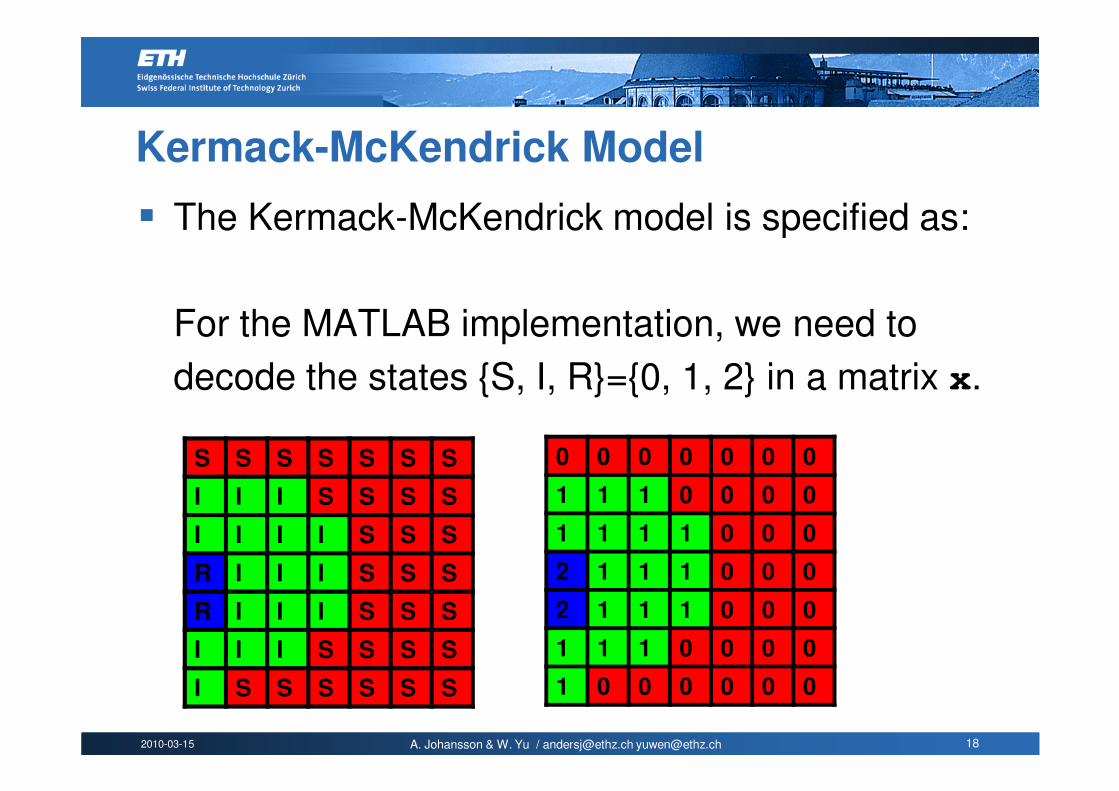
� The Kermack-McKendrick model is specified as:
For the MATLAB implementation, we need to
decode the states {S, I, R}={0, 1, 2} in a matrix x.
S S S S S S S
I I I S S S S
I I I I S S S
R I I I S S S
R I I I S S S
I I I S S S S
I S S S S S S
0 0 0 0 0 0 0
1 1 1 0 0 0 0
1 1 1 1 0 0 0
2 1 1 1 0 0 0
2 1 1 1 0 0 0
1 1 1 0 0 0 0
1 0 0 0 0 0 0
2010-03-15 A. Johansson & W. Yu / [email protected] [email protected] 19
Kermack-McKendrick Model
� The Kermack-McKendrick model is specified as:
We now define a 2-dimensional cellular-
automaton, by defining a grid (matrix) x, where
each of the cells is in one of the states:
� 0: Susceptible
� 1: Infected
� 2: Recovered
2010-03-15 A. Johansson & W. Yu / [email protected] [email protected] 20
Kermack-McKendrick Model
� The Kermack-McKendrick model is specified as:
At each time step, the cells can change states
according to:
� A Susceptible individual can be infected by an
Infected neighbor with probability β, i.e. State 0 -> 1,
with probability β.
� An individual can recover from an infection with
probability γ, i.e. State 1 -> 2, with probability γ.
2010-03-15 A. Johansson & W. Yu / [email protected] [email protected] 21
Cellular-Automaton Implementation
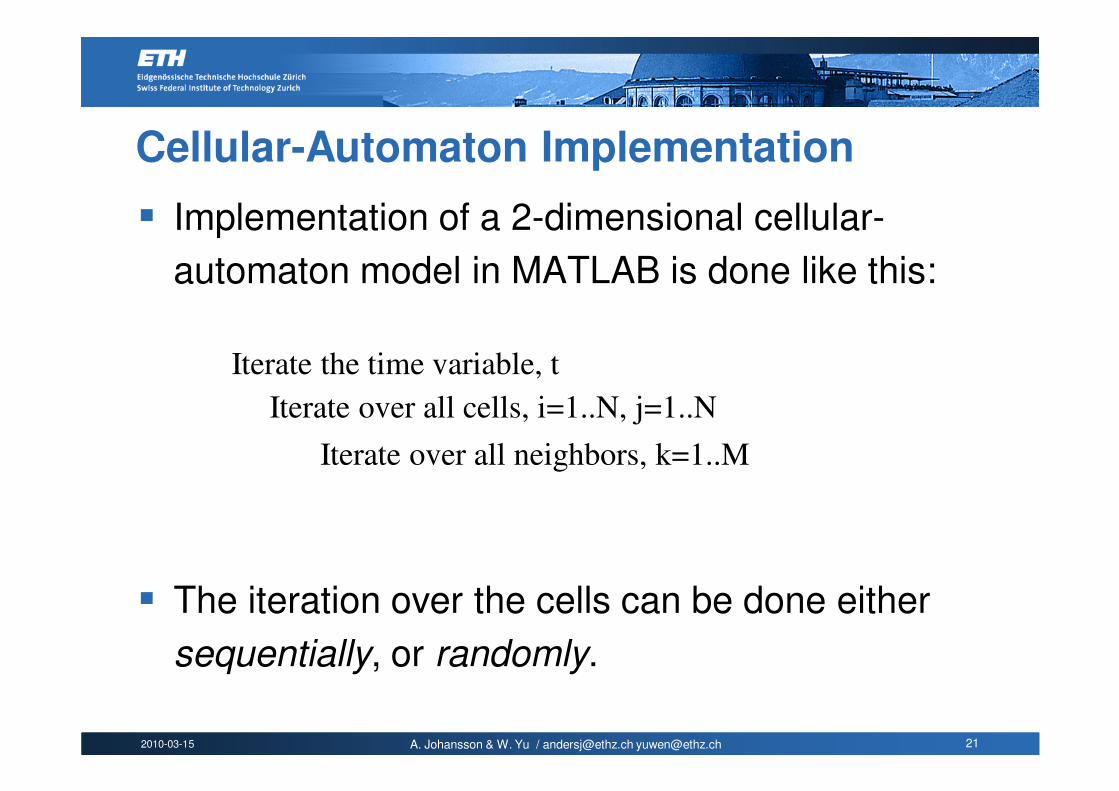
� Implementation of a 2-dimensional cellular-
automaton model in MATLAB is done like this:
� The iteration over the cells can be done either
sequentially, or randomly.
Iterate the time variable, t
Iterate over all cells, i=1..N, j=1..N
Iterate over all neighbors, k=1..M

2010-03-15 A. Johansson & W. Yu / [email protected] [email protected] 22
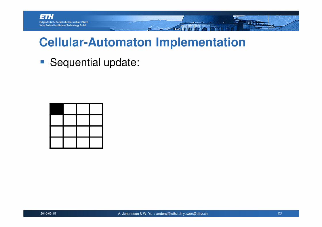
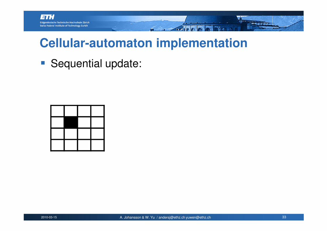
Cellular-Automaton Implementation
� Sequential update:
2010-03-15 A. Johansson & W. Yu / [email protected] [email protected] 23
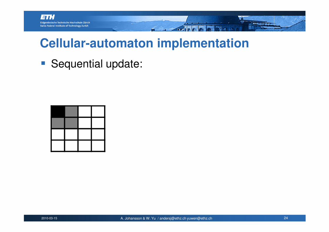
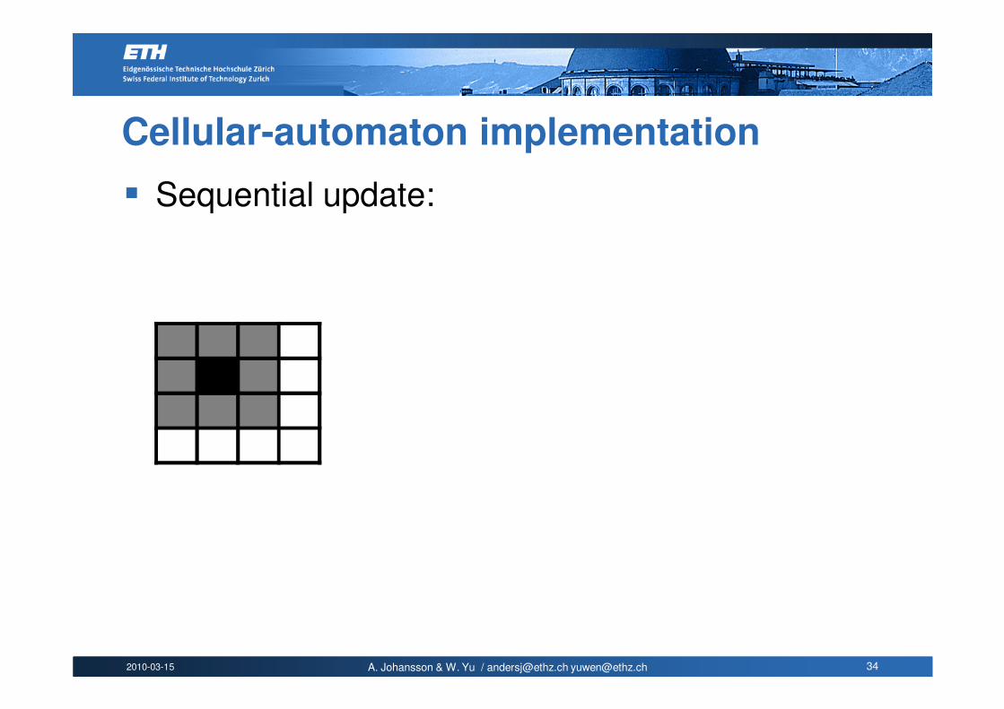
Cellular-Automaton Implementation
� Sequential update:
2010-03-15 A. Johansson & W. Yu / [email protected] [email protected] 24
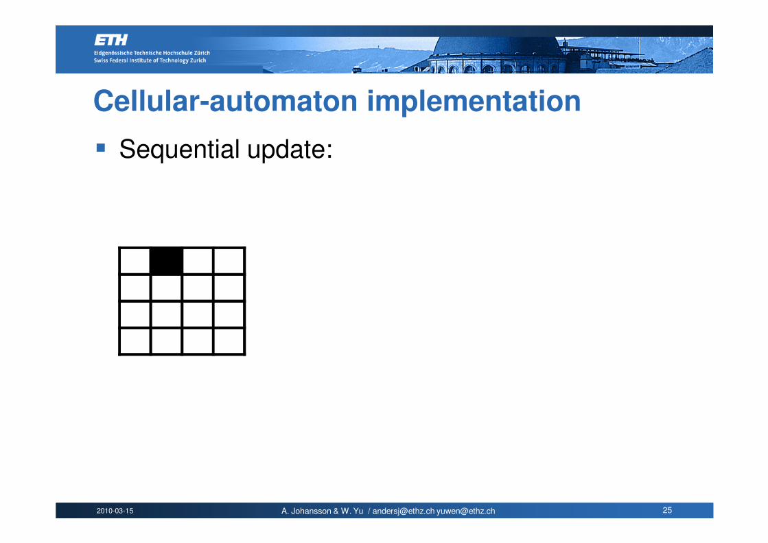
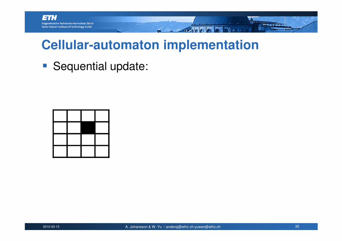
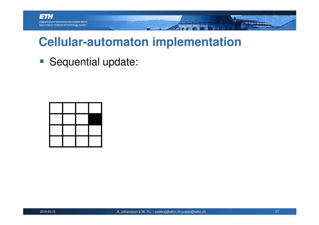
Cellular-automaton implementation
� Sequential update:
2010-03-15 A. Johansson & W. Yu / [email protected] [email protected] 25
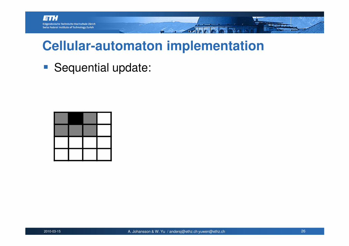
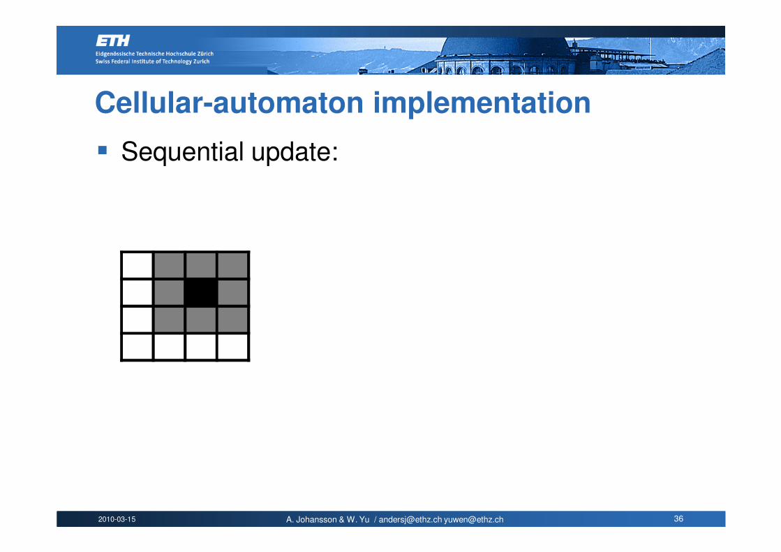
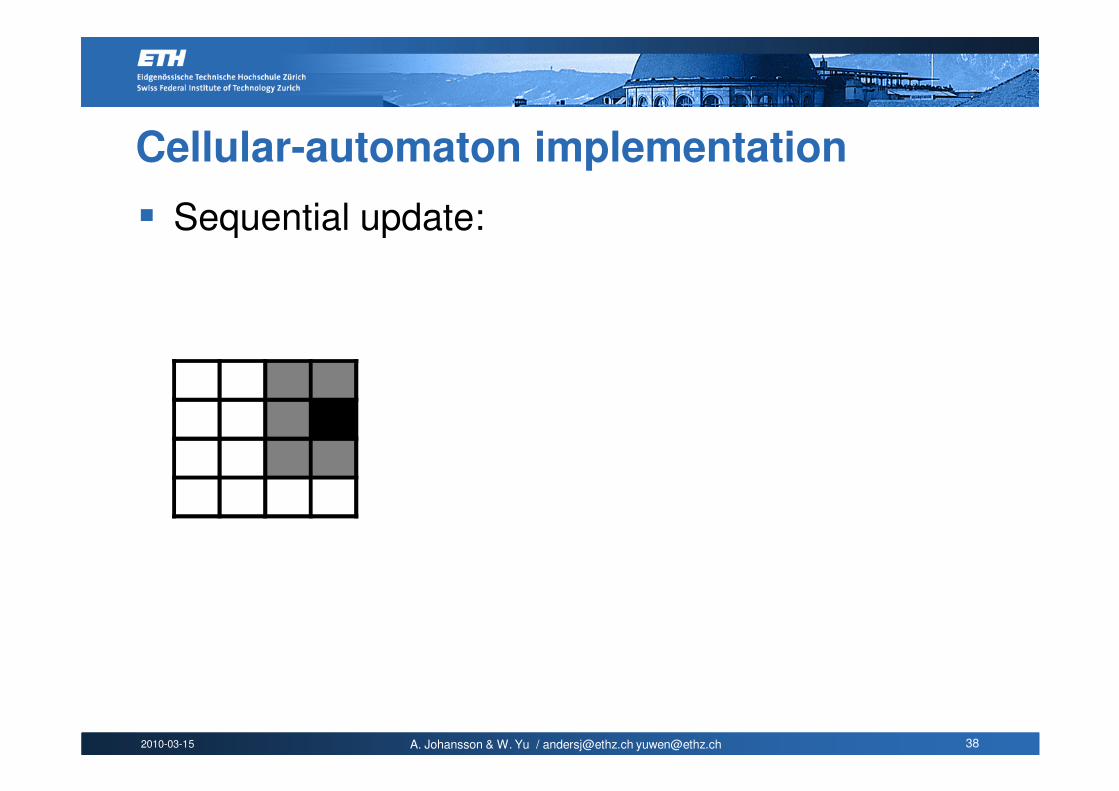
Cellular-automaton implementation
� Sequential update:
2010-03-15 A. Johansson & W. Yu / [email protected] [email protected] 26
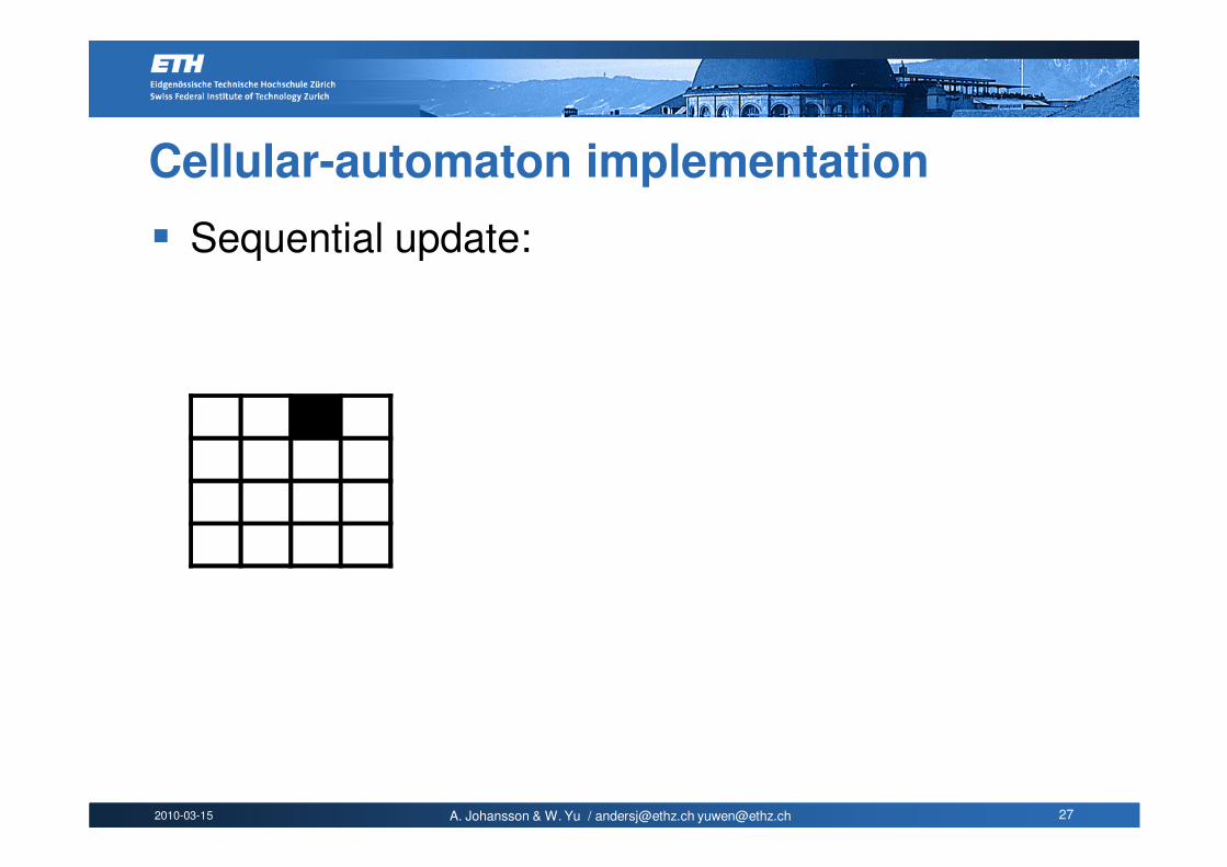
Cellular-automaton implementation
� Sequential update:
2010-03-15 A. Johansson & W. Yu / [email protected] [email protected] 27
Cellular-automaton implementation
� Sequential update:

2010-03-15 A. Johansson & W. Yu / [email protected] [email protected] 28
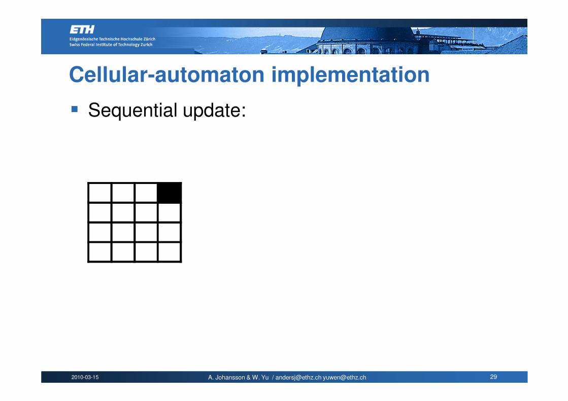
Cellular-automaton implementation
� Sequential update:
2010-03-15 A. Johansson & W. Yu / [email protected] [email protected] 29
Cellular-automaton implementation
� Sequential update:
2010-03-15 A. Johansson & W. Yu / [email protected] [email protected] 30
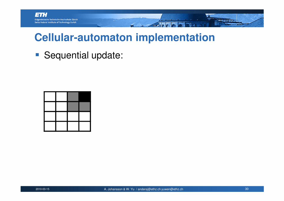
Cellular-automaton implementation
� Sequential update:

2010-03-15 A. Johansson & W. Yu / [email protected] [email protected] 31
Cellular-automaton implementation
� Sequential update:
2010-03-15 A. Johansson & W. Yu / [email protected] [email protected] 32
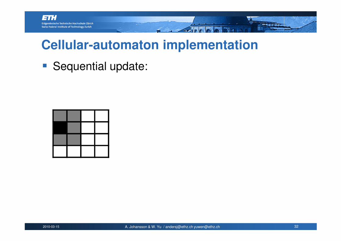
Cellular-automaton implementation
� Sequential update:
2010-03-15 A. Johansson & W. Yu / [email protected] [email protected] 33
Cellular-automaton implementation
� Sequential update:
2010-03-15 A. Johansson & W. Yu / [email protected] [email protected] 34
Cellular-automaton implementation
� Sequential update:
2010-03-15 A. Johansson & W. Yu / [email protected] [email protected] 35
Cellular-automaton implementation
� Sequential update:
2010-03-15 A. Johansson & W. Yu / [email protected] [email protected] 36
Cellular-automaton implementation
� Sequential update:
2010-03-15 A. Johansson & W. Yu / [email protected] [email protected] 37
Cellular-automaton implementation
� Sequential update:
2010-03-15 A. Johansson & W. Yu / [email protected] [email protected] 38
Cellular-automaton implementation
� Sequential update:

2010-03-15 A. Johansson & W. Yu / [email protected] [email protected] 39
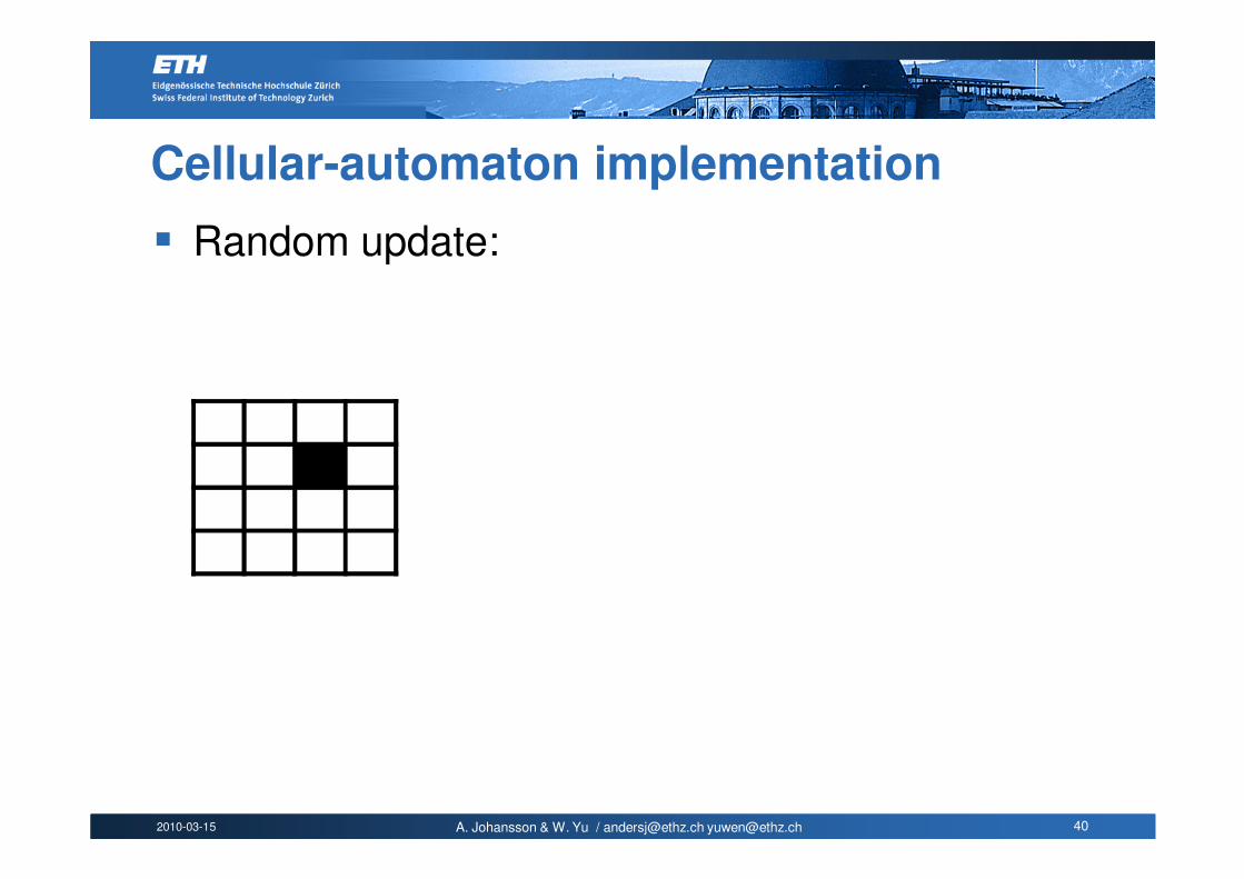
Cellular-automaton implementation
� Random update:
2010-03-15 A. Johansson & W. Yu / [email protected] [email protected] 40
Cellular-automaton implementation
� Random update:

2010-03-15 A. Johansson & W. Yu / [email protected] [email protected] 41
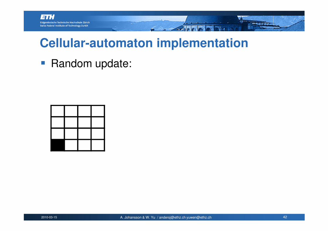
Cellular-automaton implementation
� Random update:
2010-03-15 A. Johansson & W. Yu / [email protected] [email protected] 42
Cellular-automaton implementation
� Random update:
2010-03-15 A. Johansson & W. Yu / [email protected] [email protected] 43
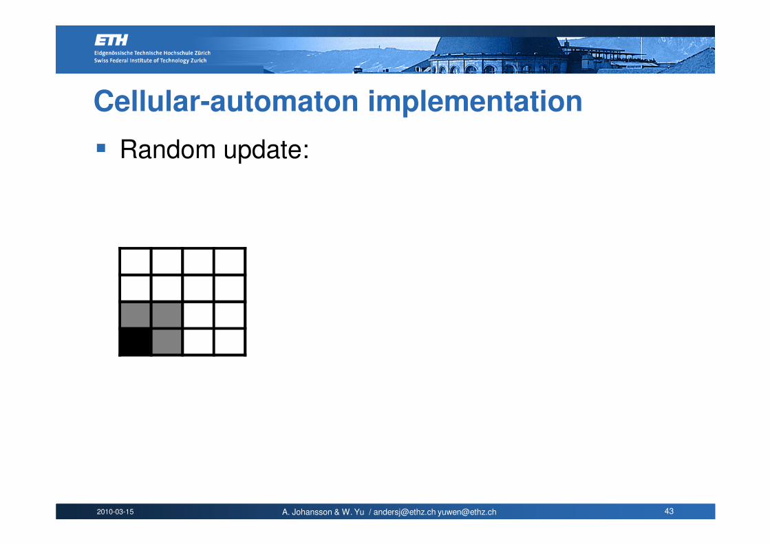
Cellular-automaton implementation
� Random update:
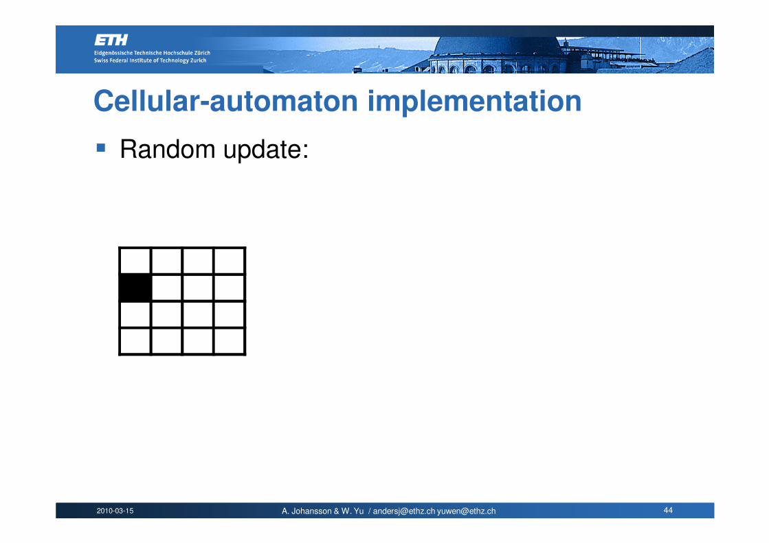
2010-03-15 A. Johansson & W. Yu / [email protected] [email protected] 44
Cellular-automaton implementation
� Random update:
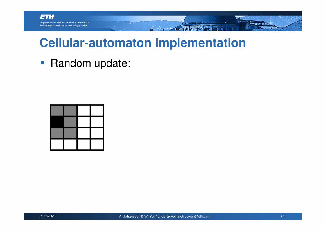
2010-03-15 A. Johansson & W. Yu / [email protected] [email protected] 45
Cellular-automaton implementation
� Random update:

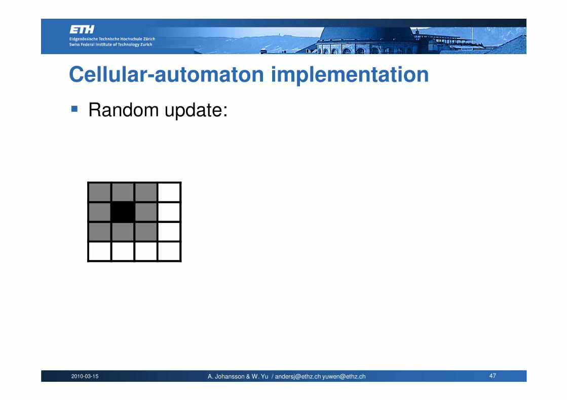
2010-03-15 A. Johansson & W. Yu / [email protected] [email protected] 46
Cellular-automaton implementation
� Random update:
2010-03-15 A. Johansson & W. Yu / [email protected] [email protected] 47
Cellular-automaton implementation
� Random update:
2010-03-15 A. Johansson & W. Yu / [email protected] [email protected] 48
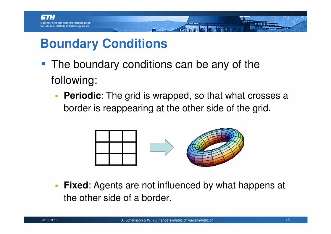
Boundary Conditions
� The boundary conditions can be any of the
following:
� Periodic: The grid is wrapped, so that what crosses a
border is reappearing at the other side of the grid.
� Fixed: Agents are not influenced by what happens at
the other side of a border.
2010-03-15 A. Johansson & W. Yu / [email protected] [email protected] 49
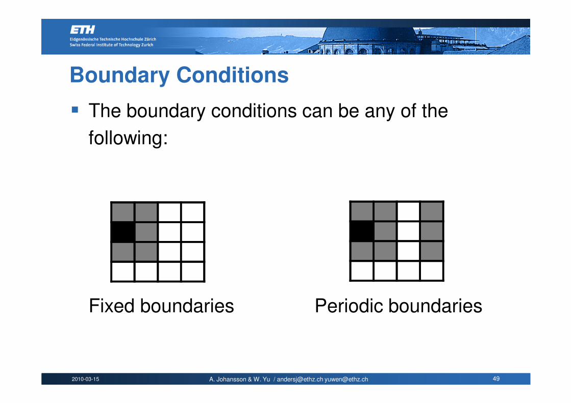
Boundary Conditions
� The boundary conditions can be any of the
following:
Fixed boundaries Periodic boundaries
2010-03-15 A. Johansson & W. Yu / [email protected] [email protected] 50
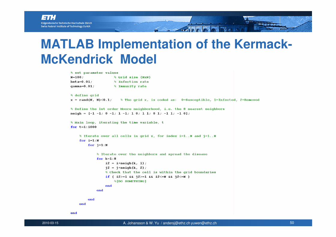
MATLAB Implementation of the Kermack-McKendrick Model
2010-03-15 A. Johansson & W. Yu / [email protected] [email protected] 51
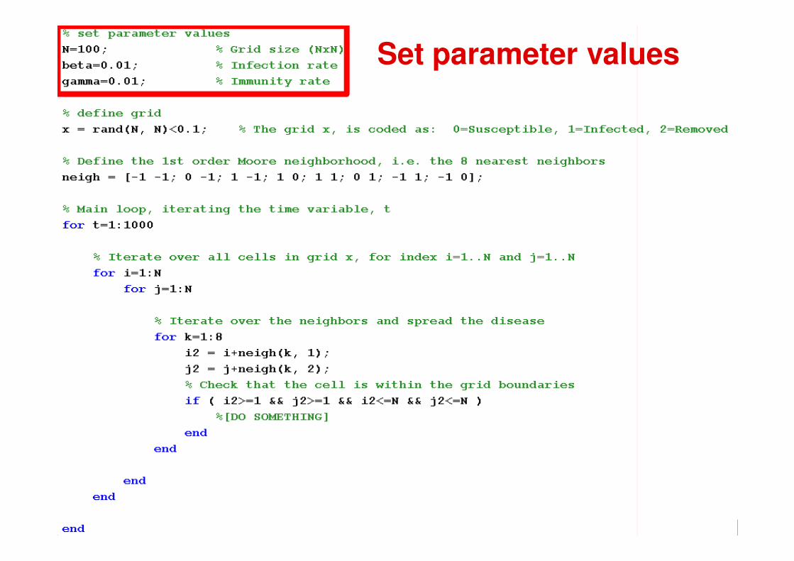
MATLAB implementation
Set parameter values
2010-03-15 A. Johansson & W. Yu / [email protected] [email protected] 52
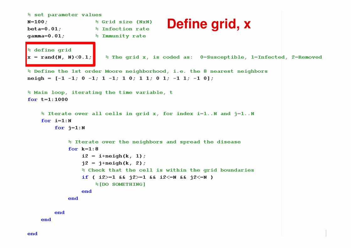
MATLAB implementation
Define grid, x
2010-03-15 A. Johansson & W. Yu / [email protected] [email protected] 53
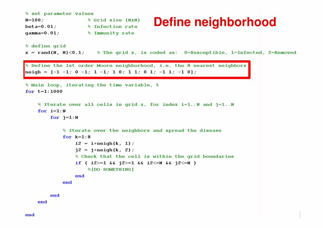
MATLAB implementation
Define neighborhood
2010-03-15 A. Johansson & W. Yu / [email protected] [email protected] 54
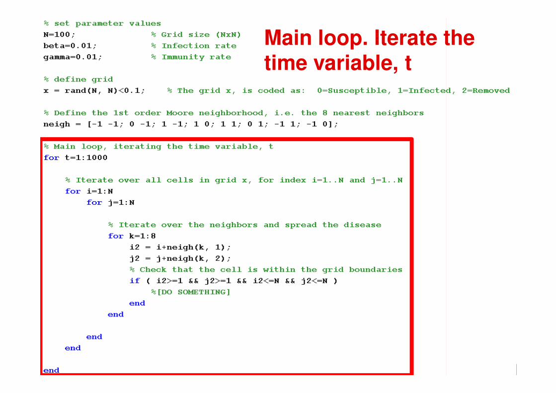
MATLAB implementation
Main loop. Iterate the time variable, t
2010-03-15 A. Johansson & W. Yu / [email protected] [email protected] 55
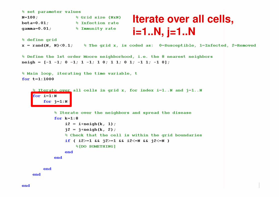
MATLAB implementation
Iterate over all cells, i=1..N, j=1..N
2010-03-15 A. Johansson & W. Yu / [email protected] [email protected] 56
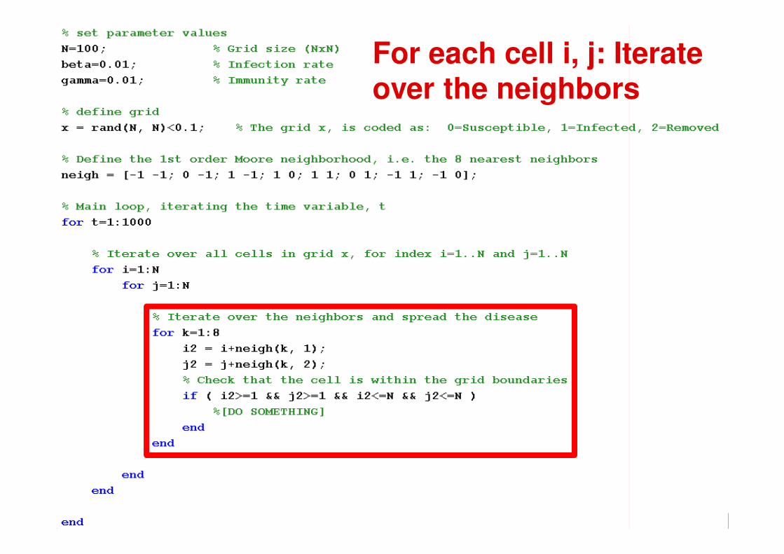
MATLAB implementation
For each cell i, j: Iterate over the neighbors
2010-03-15 A. Johansson & W. Yu / [email protected] [email protected] 57
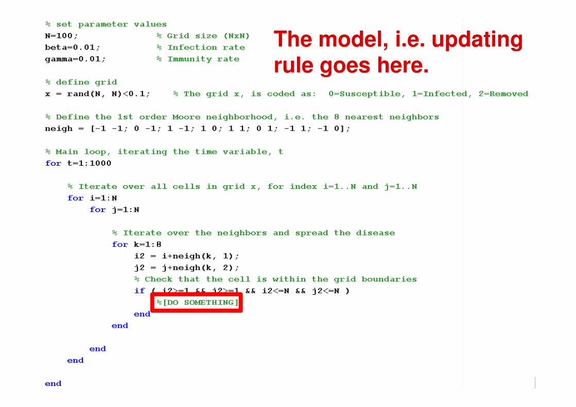
MATLAB implementation
The model, i.e. updating rule goes here.
2010-03-15 A. Johansson & W. Yu / [email protected] [email protected] 58
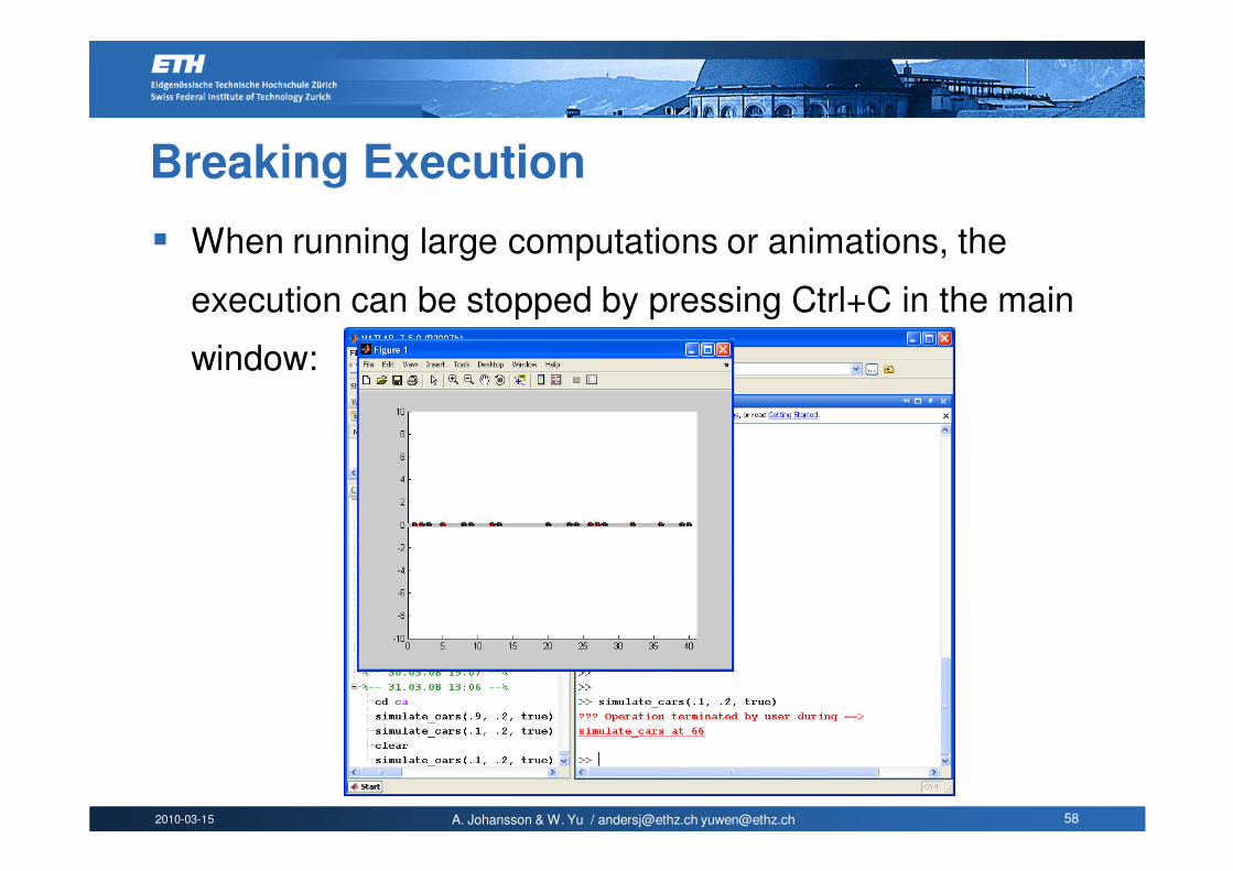
Breaking Execution
� When running large computations or animations, the
execution can be stopped by pressing Ctrl+C in the main
window:
2010-03-15 A. Johansson & W. Yu / [email protected] [email protected] 59
Projects
� Implementation of a model from the Social-
Science literature into MATLAB.
� Carried out in pairs (Indicate which sections or tasks have
been done by whom, since the grade will be individual.)
� The projects should be
� handed in as a 20-30 pages report, and
� be presented orally as a 10-minute talk.
� Please use the report template on
www.soms.ethz.ch/matlab/
2010-03-15 A. Johansson & W. Yu / [email protected] [email protected] 60
Project Report
� The report should be accompanied by:
1. MATLAB code, well documented and well structured with comments in the code. The code will later on be put on a web page and be publically available.
2. Documentation of the MATLAB code. A description of how the code works and how to use it.
3. All additional references that have been used should be handed in as pdf files.
2010-03-15 A. Johansson & W. Yu / [email protected] [email protected] 61
Project Topics
� On www.soms.ethz.ch/matlab/ you will find one
or several papers belonging to each of the
project topics.
� However, it is strongly encouraged to search for
similar papers on scholar.google.com
� It is also encouraged to come up with new
extensions and modifications of the model, as
well as coming up with your own topics and
models.
2010-03-15 A. Johansson & W. Yu / [email protected] [email protected] 62
Project Topics (2)
� On www.soms.ethz.ch/matlab/ you will find
project reports from FS 2008, FS 2009, and HS
2009.
� If you choose the same topic as one of the
projects from previous years, you have to come
up with an extension or a new direction of the
project.
2010-03-15 A. Johansson & W. Yu / [email protected] [email protected] 63
Projects
� Within one week, a small summary (less than
half an A4 page) should be sent by email. This
summary should include a brief plan which
model to implement, what to simulate and which
kind of results to expect.
� It should be sent to:
[email protected] and [email protected]
� The purpose is to get feedback and make sure
that the project will develop in the right direction.
2010-03-15 A. Johansson & W. Yu / [email protected] [email protected] 64
Projects – Summary
1. Find somebody to work with.
2. Have a look at the projects on:
www.soms.ethz.ch/matlab/
3. When you have found an interesting topic, inform
us and we will put you on the projects list.
4. Within one week, send us ([email protected] and
[email protected]) a short plan on your project
(chosen model, expected results, extensions, ...).
2010-03-15 A. Johansson & W. Yu / [email protected] [email protected] 65
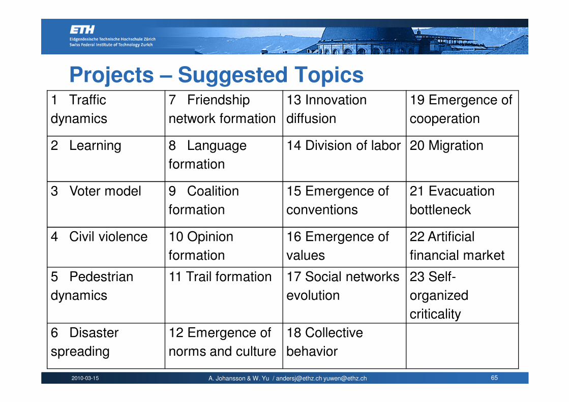
Projects – Suggested Topics1 Traffic
dynamics
7 Friendship
network formation
13 Innovation
diffusion
19 Emergence of
cooperation
2 Learning 8 Language
formation
14 Division of labor 20 Migration
3 Voter model 9 Coalition
formation
15 Emergence of
conventions
21 Evacuation
bottleneck
4 Civil violence 10 Opinion
formation
16 Emergence of
values
22 Artificial
financial market
5 Pedestrian
dynamics
11 Trail formation 17 Social networks
evolution
23 Self-
organized
criticality
6 Disaster
spreading
12 Emergence of
norms and culture
18 Collective
behavior
2010-03-15 A. Johansson & W. Yu / [email protected] [email protected] 66
Exercise 1
� Download the files draw_car.m and
simulate_cars.m from the course web page,
www.soms.ethz.ch/matlab
Investigate how the flow (moving vehicles per
time step) depends on the density (occupancy
0%..100%) in the simulator. This relation is
called the fundamental diagram in transportation
engineering.
2010-03-15 A. Johansson & W. Yu / [email protected] [email protected] 67
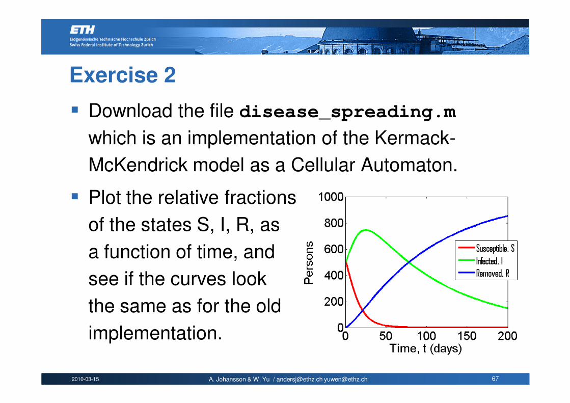
Exercise 2
� Download the file disease_spreading.m
which is an implementation of the Kermack-
McKendrick model as a Cellular Automaton.
� Plot the relative fractions
of the states S, I, R, as
a function of time, and
see if the curves look
the same as for the old
implementation.
2010-03-15 A. Johansson & W. Yu / [email protected] [email protected] 68
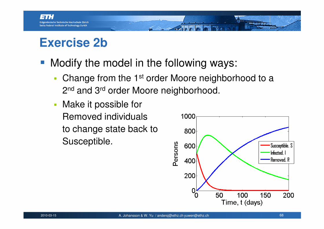
Exercise 2b
� Modify the model in the following ways:
� Change from the 1st order Moore neighborhood to a
2nd and 3rd order Moore neighborhood.
� Make it possible for
Removed individuals
to change state back to
Susceptible.
Top Related