


Languages
Pages
Legal

191 For free distributionFor free distribution190
7 Electronic Spreadsheet
In this chapter you will learn
² fundamental functions and operations of spreadsheets ² identifying the components of a worksheet ² entering and editing data in a worksheet ² simple mathematical operators and building a formula using values ² use of function and cell address for writing formulae ² formatting a worksheet ² use of relative and absolute cell addresses, ² creating charts.
7.1 Introduction Perhaps in our day-to-day life or at work we need to perform calculations. We use various methods to perform such calculations. Depending on the nature of calculations we use our fingers or mental calculations to perform simple calculations while we use calculators or paper based systems to compute complex calculations. In order to do calculations easily and accurately let us learn how electronic spreadsheets can be used.
We usually use a square ruled book to perform systematic calculations. Every page in this book consists of pages with rows and columns. Electronic Spreadsheets which consist of multiples of rows and columns based on this model of square ruled books.
191 For free distributionFor free distribution190
Using Electronic Spreadsheets we can accurately and efficiently perform the following activities:
• Simple and complex calculations• Presentation of data in charts• Show data in ascending and descending order• Segregate only the required data• Check the validity of data• Protection of data using passwords• Saving for future use
7.1.1 Electronic Spreadsheet Application Software
The table 7.1 below illustrates some of the Electronic Spreadsheet Application Software developed by different companies.
Table 7.1 - Some Spreadsheet Applications and the and organizations
Software Company Excel Microsoft Corporation Numbers Apple Inc Libreoffice Calc The Document Foundation Openoffice Calc Apache Foundation
7.1.2 Using Spreadsheet Software
Out of the many spreadsheet software, we discuss only about Microsoft Office Excel 2010 and LibreOffice Calc in this unit. Please note that the method of starting an spreadsheet software may vary according to the operating system and its versions.
For Microsoft Office Excel 2010
Start → Programs→ Microsoft Office→ Microsoft Office Excel 2010
For LibreOffice Calc
Start → Programs → LibreOffice LibreOffice Calc →
193 For free distributionFor free distribution192
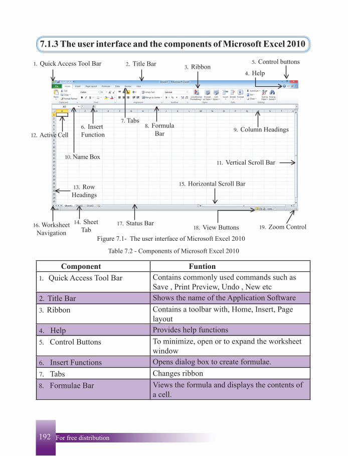
7.1.3 The user interface and the components of Microsoft Excel 2010
10' kdu fldgqj
Name Box
6' Insert Function
7' Tabs8' Formula
Bar 9' Column Headings
1' Quick Access Tool Bar 2' Title Bar 3' Ribbon
4' Help
5' Control buttons
12' Active Cell
13' Row Headings
14' Sheet Tab
11' Vertical Scroll Bar
15' Horizontal Scroll Bar
19' Zoom Control18' View Buttons17' Status Bar16' Worksheet Navigation
10' Name Box
Figure 7.1- The user interface of Microsoft Excel 2010
Table 7.2 - Components of Microsoft Excel 2010
Component Funtion1' Quick Access Tool Bar Contains commonly used commands such as
Save , Print Preview, Undo , New etc2' Title Bar Shows the name of the Application Software3' Ribbon Contains a toolbar with, Home, Insert, Page
layout 4' Help Provides help functions5' Control Buttons To minimize, open or to expand the worksheet
window6' Insert Functions Opens dialog box to create formulae.7' Tabs Changes ribbon8' Formulae Bar Views the formula and displays the contents of
a cell.
193 For free distributionFor free distribution192
9' Column Heading Shows column name10' Name Box Shows active cell address11' Vertical Scroll Bar Scrolls the worksheet vertically12' Active Cell Displays the cell in which data is entered13' Row Heading Shows row number14' Sheet Tabs Represents the worksheet15' Horizontal Scroll Bar Scrolls the worksheet horizontally16' Sheet Tab Scroll Button Changes the worksheet17' Status Bar Displays the status of the worksheet18' View Button Enables to change the view of the worksheet19' Zoom Control Zooms in or zooms out the view of a
worksheets
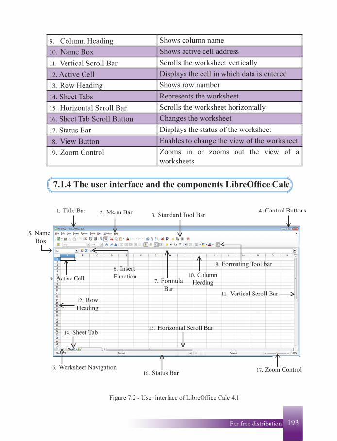
7.1.4 The user interface and the components LibreOffice Calc
3' Standard Tool Bar 2' Menu Bar1' Title Bar
5' Name Box
9' Active Cell 6' Insert Function
7' Formula Bar
11' Vertical Scroll Bar
13' Horizontal Scroll Bar
16' Status Bar15' Worksheet Navigation
12' Row Heading
17' Zoom Control
4' Control Buttons
8' Formating Tool bar
14' Sheet Tab
10' Column Heading
Figure 7.2 - User interface of LibreOffice Calc 4.1
195 For free distributionFor free distribution194
Component Funtion1' Title Bar Shows the name of the application software2' Menu bar Helps to select commands3' Standard tool bar Useful to select standard tools4' Control buttons Minimizes, opens or to maximize the worksheet
window5' Name box Shows the address of the active cell 6' Insert Functions Opens dialog box to make formulae.7' Formulae bar To view formula and display the contents of a
cell. 8' Formatting tool bar Helps to format worksheet9' Active cell Displays cell in which data is entered10' Column heading Shows column name11' Vertical scroll bar Scrolls worksheet vertically12' Row heading Shows row number13' Horizontal scroll bar Scrolls worksheet horizontally14' Sheet tabs Represents worksheet.15' Tab scroll button Changes worksheet.16' Status Bar Displays the status of worksheet.17' Zoom Control Zooms in or zooms out view of a worksheet
7.1.5 Worksheet
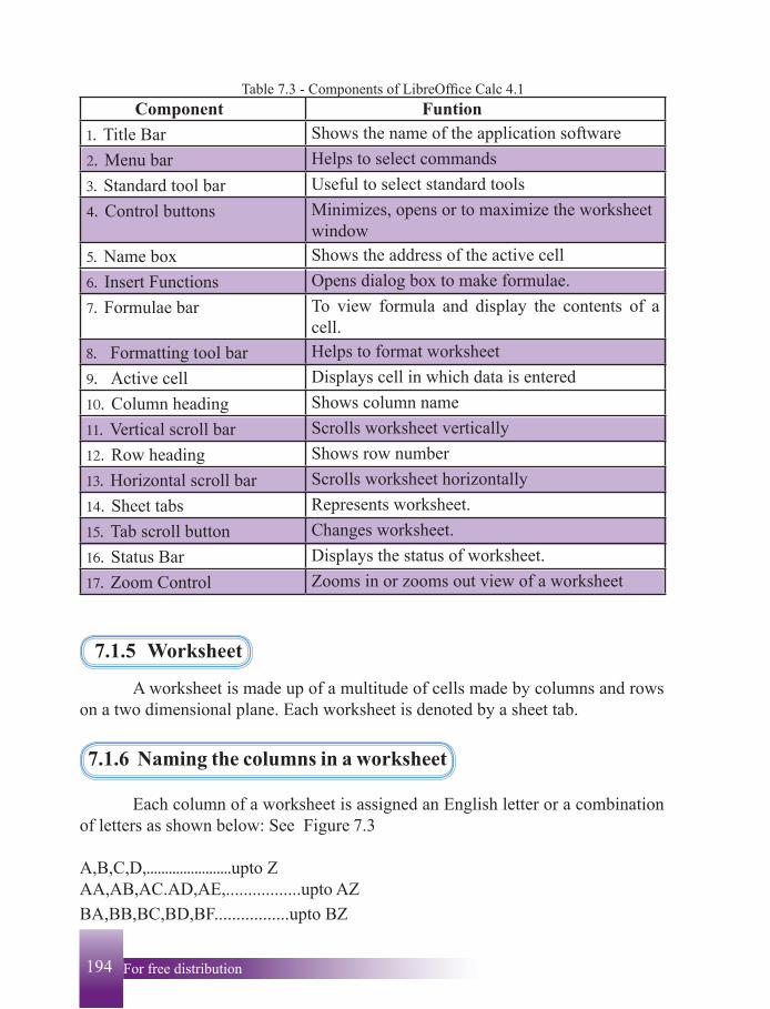
A worksheet is made up of a multitude of cells made by columns and rows on a two dimensional plane. Each worksheet is denoted by a sheet tab.
7.1.6 Naming the columns in a worksheet
Each column of a worksheet is assigned an English letter or a combination of letters as shown below: See Figure 7.3
A,B,C,D,'''''''''''''''''''''''upto Z AA,AB,AC.AD,AE,.................upto AZ
BA,BB,BC,BD,BF.................upto BZ
Table 7.3 - Components of LibreOffice Calc 4.1
195 For free distributionFor free distribution194
7.1.7 Naming the rows in a worksheet
Each row of a worksheet is assigned a row number as 1,2,3,4,5... etc as shown below: See Figure 7.3
Usually the number of rows and columns of a worksheet is a power of two.
Worksheet application Number of rows Number of columns
Microsoft Excel 2003 65536 ^216& 256 ^28&
Microsoft Excel 2007$2010 1048576 ^220& 16384 ^214&
LibreOffice Calc 4'1 1048576 ^220& 1024 ^210&
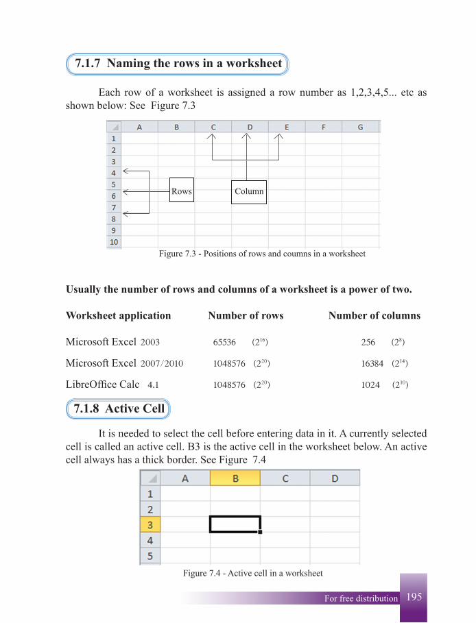
7.1.8 Active Cell
It is needed to select the cell before entering data in it. A currently selected cell is called an active cell. B3 is the active cell in the worksheet below. An active cell always has a thick border. See Figure 7.4
Figure 7.4 - Active cell in a worksheet
Rows Column
Figure 7.3 - Positions of rows and coumns in a worksheet
197 For free distributionFor free distribution196
7.2 Scrolling in a worksheet
In order to enter data the cell, it should be selected. Active cell in a worksheet can be moved and selected by the keys or a combination of keys.
Key/combination of keys Result
Arrow keys Move a single cell in any direction (left, right, up, down)Ctrl + Arrow Keys Moves the cell to the end of the data range in a particular directionHome Moves to column A along the row where the active cell isCtrl + Home Moves the cell to A1 position
Ctrl + End Moves to bottom right cell of the data range
Page Up Moves the worksheet one screen upPage Down Moves the worksheet one screen down
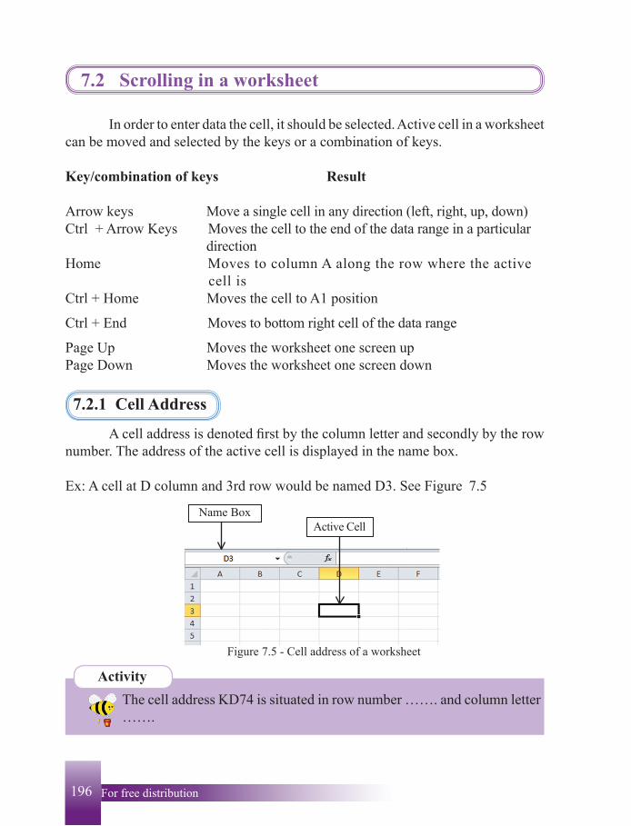
7.2.1 Cell Address
A cell address is denoted first by the column letter and secondly by the row number. The address of the active cell is displayed in the name box.
Ex: A cell at D column and 3rd row would be named D3. See Figure 7.5
Name Box Active Cell
Figure 7.5 - Cell address of a worksheet
Activity The cell address KD74 is situated in row number ……. and column letter
…….
197 For free distributionFor free distribution196
7.2.2 Range of Cells
A block of adjacent cells in a worksheet which is highlighted or selected is called a range of cells. Observe the worksheets below.
Figure 7.6 - A range of cells in a column (B2: B5)
This range of cells consists of the cells namely B2,B3,B4,B5. The range of cells starts in B2 and ending in B5. Column letter is constant in a cell range along a column. The cell range in figure 7.6 is represented by B2:B5.
Figure 7.7 - A range of cell in a row
This range of cells is represented as A3:C3. The range in Figure 7.7 consists of the cells A3,B3,C3. See Figure 7.7. This range of cells is represented as A3:C3. Row number is constant in a cell range along a row. For this cell range in Figure 7.7, cells; B2, B3, B4, C2, C3, and C4 are included.
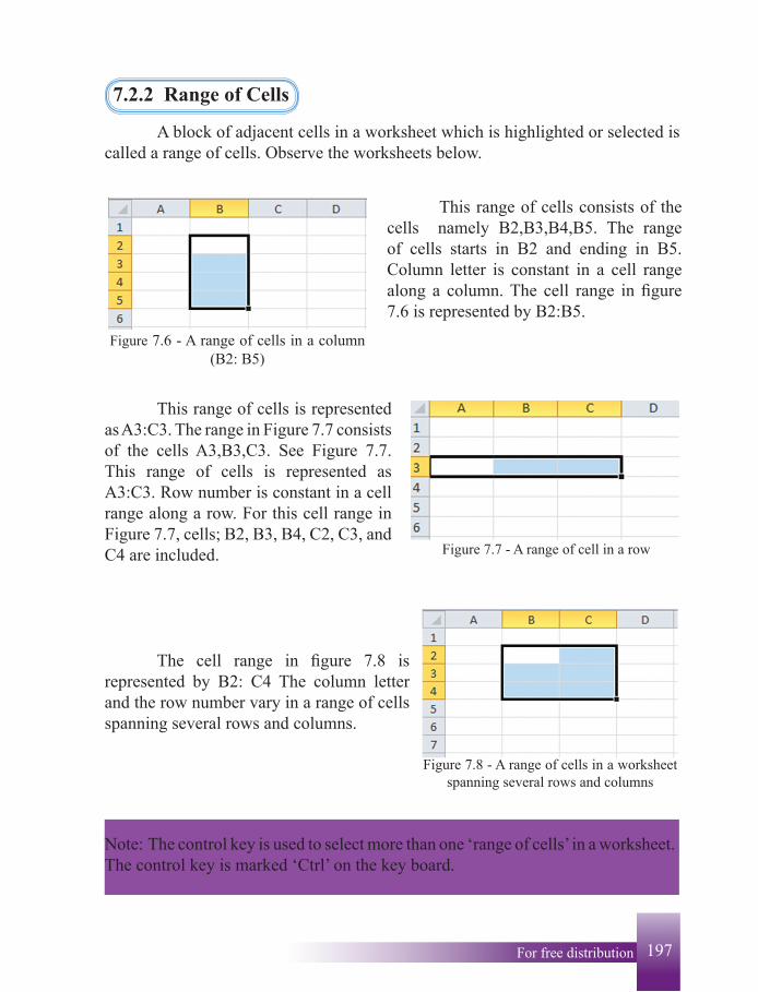
The cell range in figure 7.8 is represented by B2: C4 The column letter and the row number vary in a range of cells spanning several rows and columns.
Figure 7.8 - A range of cells in a worksheet spanning several rows and columns
Note: The control key is used to select more than one ‘range of cells’ in a worksheet. The control key is marked ‘Ctrl’ on the key board.
199 For free distributionFor free distribution198
Activity
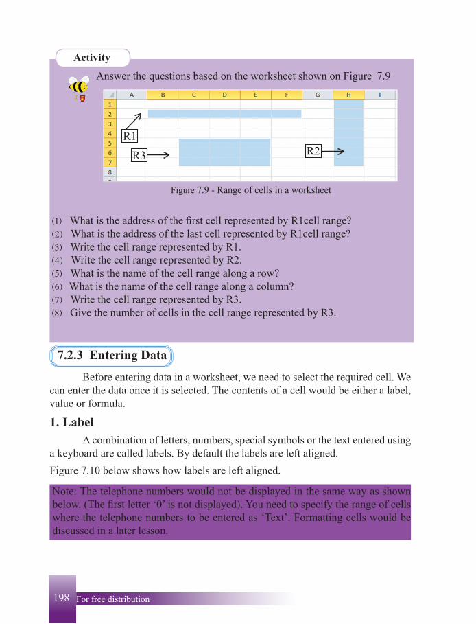
Answer the questions based on the worksheet shown on Figure 7.9
^1& What is the address of the first cell represented by R1cell range?^2& What is the address of the last cell represented by R1cell range?^3& Write the cell range represented by R1.^4& Write the cell range represented by R2.^5& What is the name of the cell range along a row?^6& What is the name of the cell range along a column?^7& Write the cell range represented by R3.^8& Give the number of cells in the cell range represented by R3.
R1R2R3
Figure 7.9 - Range of cells in a worksheet
7.2.3 Entering Data
Before entering data in a worksheet, we need to select the required cell. We can enter the data once it is selected. The contents of a cell would be either a label, value or formula.
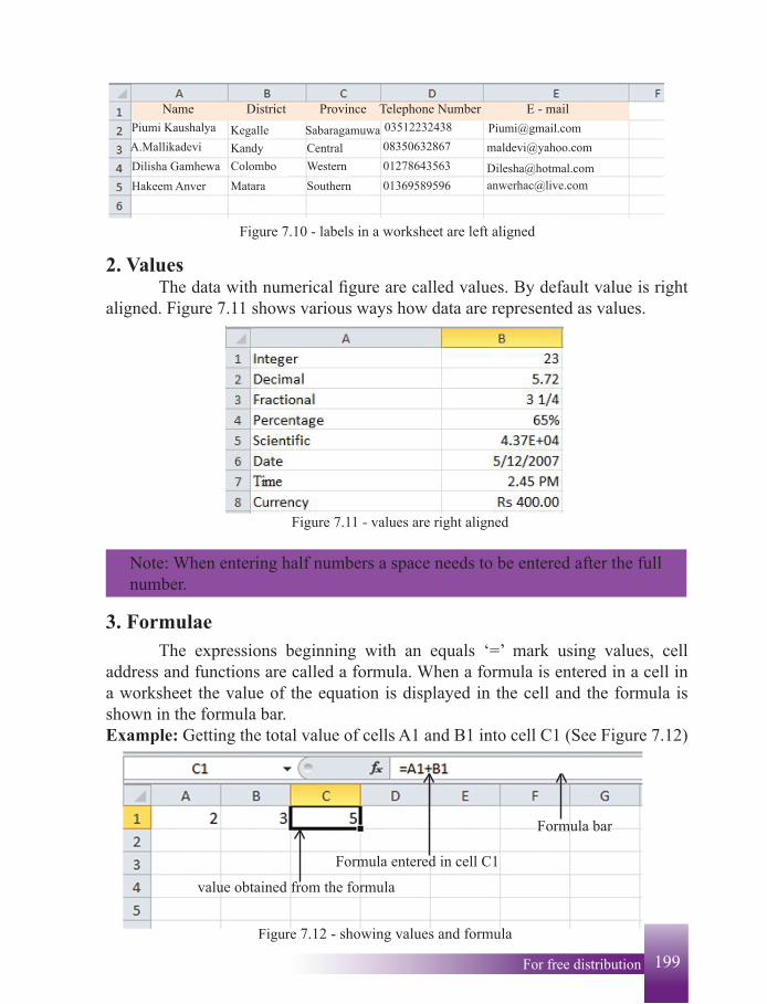
1. Label A combination of letters, numbers, special symbols or the text entered using a keyboard are called labels. By default the labels are left aligned. Figure 7.10 below shows how labels are left aligned.
Note: The telephone numbers would not be displayed in the same way as shown below. (The first letter ‘0’ is not displayed). You need to specify the range of cells where the telephone numbers to be entered as ‘Text’. Formatting cells would be discussed in a later lesson.
199 For free distributionFor free distribution198
Figure 7.10 - labels in a worksheet are left aligned
Piumi Kaushalya [email protected] Sabaragamuwa
Name District Province E - mailTelephone Number
A.Mallikadevi [email protected] CentralDilisha Gamhewa [email protected] WesternHakeem Anver [email protected] Southern
2. Values The data with numerical figure are called values. By default value is right aligned. Figure 7.11 shows various ways how data are represented as values.
Figure 7.11 - values are right aligned
Note: When entering half numbers a space needs to be entered after the full number.
3. Formulae The expressions beginning with an equals ‘=’ mark using values, cell address and functions are called a formula. When a formula is entered in a cell in a worksheet the value of the equation is displayed in the cell and the formula is shown in the formula bar.Example: Getting the total value of cells A1 and B1 into cell C1 (See Figure 7.12)
value obtained from the formula
Formula bar
Formula entered in cell C1
Figure 7.12 - showing values and formula
201 For free distributionFor free distribution200
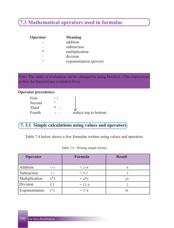
7.3 Mathematical operators used in formulae
Operator Meaning ¬ addition - subtraction * multiplication / division ^ exponentiation (power)
Note: The order of evaluation can be changed by using brackets. (The expressions within the brackets are evaluated first).
Operator precedence:
First ^ &
Second ^ Third * " $ Fourth ¬ " - reduce top to bottom.
7. 3.1 Simple calculations using values and operators
Table 7.4 below shows a few formulae written using values and operators
Table 7.4 - Writing simple formul
Operator Formula Result
Addition ^¬& = 2¬4 6
Subtraction ^-& = 5-2 3
Multiplication (*) = 4*5 20
Division (/) = 12$6 2
Exponentiation (^) = 2^4 16
201 For free distributionFor free distribution200
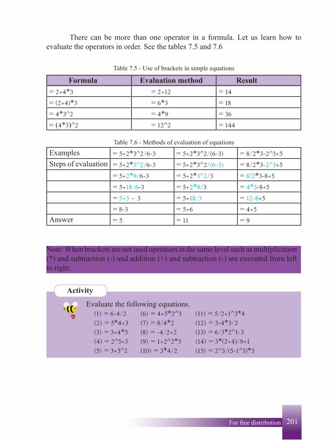
There can be more than one operator in a formula. Let us learn how to evaluate the operators in order. See the tables 7.5 and 7.6
Table 7.5 - Use of brackets in simple equations
Formula Evaluation method Result= 2¬4*3 = 2¬12 = 14= ^2¬4&*3 = 6*3 = 18= 4*3^2 = 4*9 = 36= (4*3)^2 = 12^2 = 144
Table 7.6 - Methods of evaluation of equations
Examples = 5¬2*3^2$6-3 = 5¬2*3^2$^6-3& = 8$2*3-2^3¬5Steps of evaluation = 5¬2*3^2$6-3 = 5¬2*3^2$^6-3& = 8$2*3-2^3¬5
= 5¬2*9$6-3 = 5¬2*3^2$3 = 8/2*3-8¬5= 5¬18$6-3 = 5¬2*9$3 = 4*3-8¬5= 5¬3 - 3 = 5¬18$3 = 12-8¬5= 8-3 = 5¬6 = 4¬5
Answer = 5 = 11 = 9
Note: When brackets are not used operators in the same level such as multiplication (*) and subtraction (-) and addition (+) and subtraction (-) are executed from left to right.
Activity
Evaluate the following equations. ^1& = 6-4$2 ^6& = 4¬5*2^3 ^11& = 5$2¬1^3*4 ^2& = 5*4¬3 ^7& = 8$4*2 ^12& = 3-4*3$2 ^3& = 3¬4*5 ^8& = -4$2¬2 ^13& = 6$3*2^1-3 ^4& = 2^5¬3 ^9& = 1¬2^2*3 ^14& = 3*^2¬4&$9¬1 ^5& = 3¬5^2 ^10& = 3*4$2 ^15& = 2^3$^5-1^3&*5
203 For free distributionFor free distribution202
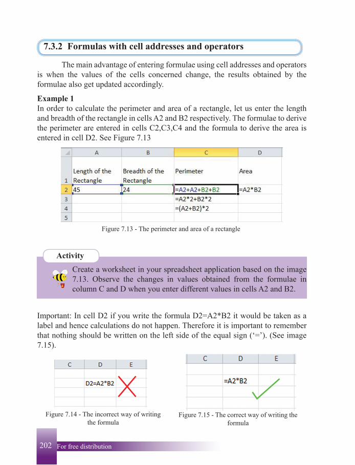
7.3.2 Formulas with cell addresses and operators
The main advantage of entering formulae using cell addresses and operators is when the values of the cells concerned change, the results obtained by the formulae also get updated accordingly.
Example 1In order to calculate the perimeter and area of a rectangle, let us enter the length and breadth of the rectangle in cells A2 and B2 respectively. The formulae to derive the perimeter are entered in cells C2,C3,C4 and the formula to derive the area is entered in cell D2. See Figure 7.13
Figure 7.13 - The perimeter and area of a rectangle
Activity
Create a worksheet in your spreadsheet application based on the image 7.13. Observe the changes in values obtained from the formulae in column C and D when you enter different values in cells A2 and B2.
Important: In cell D2 if you write the formula D2=A2*B2 it would be taken as a label and hence calculations do not happen. Therefore it is important to remember that nothing should be written on the left side of the equal sign (‘=’). (See image 7.15).
Figure 7.14 - The incorrect way of writing the formula
Figure 7.15 - The correct way of writing the formula
203 For free distributionFor free distribution202
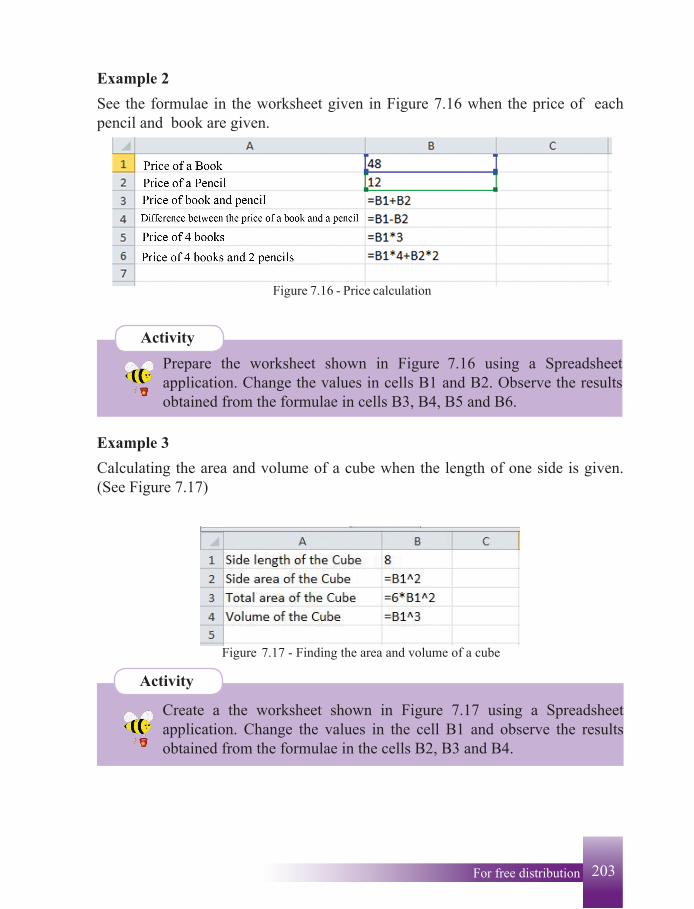
Example 2 See the formulae in the worksheet given in Figure 7.16 when the price of each pencil and book are given.
Figure 7.16 - Price calculation
Activity Prepare the worksheet shown in Figure 7.16 using a Spreadsheet application. Change the values in cells B1 and B2. Observe the results obtained from the formulae in cells B3, B4, B5 and B6.
Example 3Calculating the area and volume of a cube when the length of one side is given. (See Figure 7.17)
Figure 7.17 - Finding the area and volume of a cube
Activity
Create a the worksheet shown in Figure 7.17 using a Spreadsheet application. Change the values in the cell B1 and observe the results obtained from the formulae in the cells B2, B3 and B4.
205 For free distributionFor free distribution204
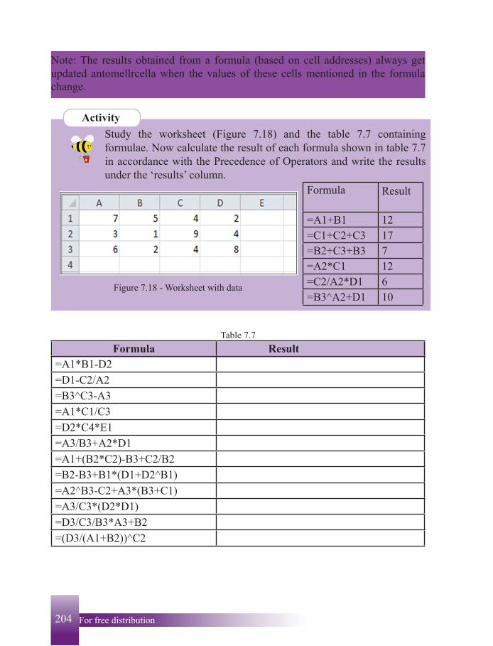
Note: The results obtained from a formula (based on cell addresses) always get updated antomellrcella when the values of these cells mentioned in the formula change.
Activity Study the worksheet (Figure 7.18) and the table 7.7 containing formulae. Now calculate the result of each formula shown in table 7.7 in accordance with the Precedence of Operators and write the results under the ‘results’ column.
Formula Result
=A1+B1 12=C1+C2+C3 17=B2+C3+B3 7=A2*C1 12=C2/A2*D1 6=B3^A2+D1 10
Figure 7.18 - Worksheet with data
Table 7.7Formula Result
=A1*B1-D2=D1-C2/A2=B3^C3-A3=A1*C1/C3=D2*C4*E1=A3/B3+A2*D1=A1+(B2*C2)-B3+C2/B2=B2-B3+B1*(D1+D2^B1)=A2^B3-C2+A3*(B3+C1)=A3/C3*(D2*D1)=D3/C3/B3*A3+B2=(D3/(A1+B2))^C2
205 For free distributionFor free distribution204
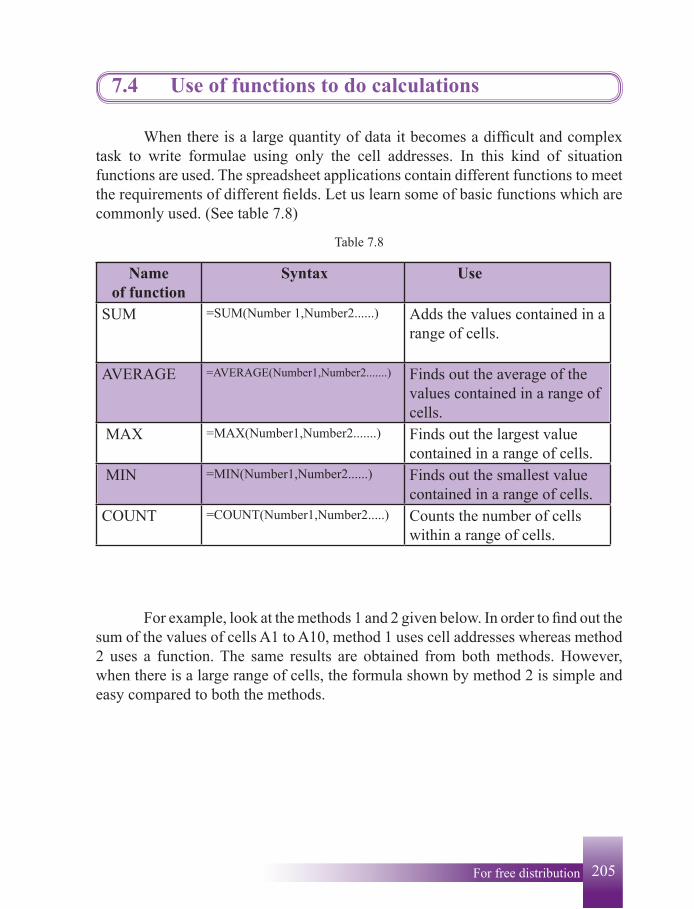
7.4 Use of functions to do calculations
When there is a large quantity of data it becomes a difficult and complex task to write formulae using only the cell addresses. In this kind of situation functions are used. The spreadsheet applications contain different functions to meet the requirements of different fields. Let us learn some of basic functions which are commonly used. (See table 7.8)
Table 7.8
Name of function
Syntax Use
SUM =SUM(Number 1,Number2......) Adds the values contained in a range of cells.
AVERAGE =AVERAGE(Number1,Number2.......) Finds out the average of the values contained in a range of cells.
MAX =MAX(Number1,Number2.......) Finds out the largest value contained in a range of cells.
MIN =MIN(Number1,Number2......) Finds out the smallest value contained in a range of cells.
COUNT =COUNT(Number1,Number2.....) Counts the number of cells within a range of cells.
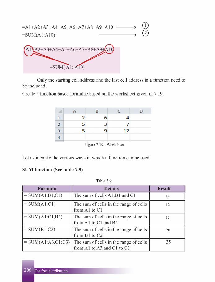
For example, look at the methods 1 and 2 given below. In order to find out the sum of the values of cells A1 to A10, method 1 uses cell addresses whereas method 2 uses a function. The same results are obtained from both methods. However, when there is a large range of cells, the formula shown by method 2 is simple and easy compared to both the methods.
207 For free distributionFor free distribution206
=A1+A2+A3+A4+A5+A6+A7+A8+A9+A10 1
=SUM(A1:A10) 2
=A1+A2+A3+A4+A5+A6+A7+A8+A9+A10
=SUM( A1: A10)
Only the starting cell address and the last cell address in a function need to be included.Create a function based formulae based on the worksheet given in 7.19.
Figure 7.19 - Worksheet
Let us identify the various ways in which a function can be used.
SUM function (See table 7.9)
Table 7.9
Formula Details Result= SUM(A1,B1,C1) The sum of cells A1,B1 and C1 12
= SUM(A1:C1) The sum of cells in the range of cells from A1 to C1
12
= SUM(A1:C1,B2) The sum of cells in the range of cells from A1 to C1 and B2
15
= SUM(B1:C2) The sum of cells in the range of cells from B1 to C2
20
= SUM(A1:A3,C1:C3) The sum of cells in the range of cells from A1 to A3 and C1 to C3
35
207 For free distributionFor free distribution206
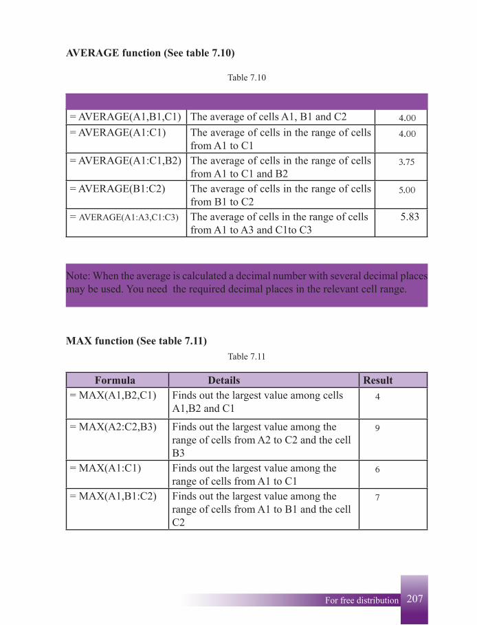
AVERAGE function (See table 7.10)
Table 7.10
Formula Details Result= AVERAGE(A1,B1,C1) The average of cells A1, B1 and C2 4'00
= AVERAGE(A1:C1) The average of cells in the range of cells from A1 to C1
4'00
= AVERAGE(A1:C1,B2) The average of cells in the range of cells from A1 to C1 and B2
3'75
= AVERAGE(B1:C2) The average of cells in the range of cells from B1 to C2
5'00
= AVERAGE(A1:A3,C1:C3) The average of cells in the range of cells from A1 to A3 and C1to C3
5.83
Note: When the average is calculated a decimal number with several decimal places may be used. You need the required decimal places in the relevant cell range.
MAX function (See table 7.11)Table 7.11
Formula Details Result= MAX(A1,B2,C1) Finds out the largest value among cells
A1,B2 and C1 4
= MAX(A2:C2,B3) Finds out the largest value among the range of cells from A2 to C2 and the cell B3
9
= MAX(A1:C1) Finds out the largest value among the range of cells from A1 to C1
6
= MAX(A1,B1:C2) Finds out the largest value among the range of cells from A1 to B1 and the cell C2
7
209 For free distributionFor free distribution208
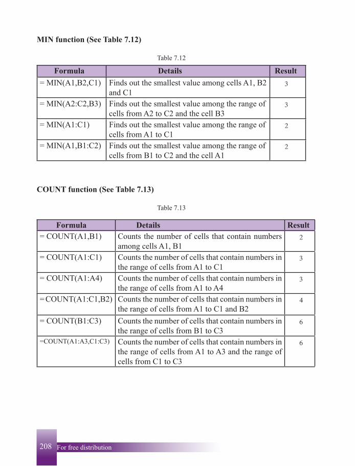
MIN function (See Table 7.12)
Table 7.12
Formula Details Result= MIN(A1,B2,C1) Finds out the smallest value among cells A1, B2
and C1 3
= MIN(A2:C2,B3) Finds out the smallest value among the range of cells from A2 to C2 and the cell B3
3
= MIN(A1:C1) Finds out the smallest value among the range of cells from A1 to C1
2
= MIN(A1,B1:C2) Finds out the smallest value among the range of cells from B1 to C2 and the cell A1
2
COUNT function (See Table 7.13)
Table 7.13
Formula Details Result= COUNT(A1,B1) Counts the number of cells that contain numbers
among cells A1, B1 2
= COUNT(A1:C1) Counts the number of cells that contain numbers in the range of cells from A1 to C1
3
= COUNT(A1:A4) Counts the number of cells that contain numbers in the range of cells from A1 to A4
3
= COUNT(A1:C1,B2) Counts the number of cells that contain numbers in the range of cells from A1 to C1 and B2
4
= COUNT(B1:C3) Counts the number of cells that contain numbers in the range of cells from B1 to C3
6
=COUNT(A1:A3,C1:C3) Counts the number of cells that contain numbers in the range of cells from A1 to A3 and the range of cells from C1 to C3
6
209 For free distributionFor free distribution208
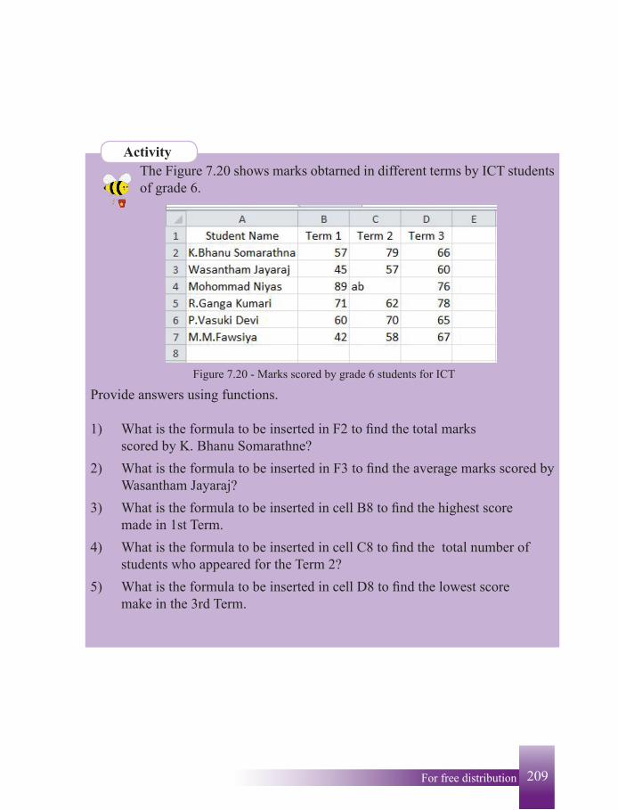
ActivityThe Figure 7.20 shows marks obtarned in different terms by ICT students of grade 6.
Provide answers using functions. 1) What is the formula to be inserted in F2 to find the total marks
scored by K. Bhanu Somarathne?2) What is the formula to be inserted in F3 to find the average marks scored by
Wasantham Jayaraj?3) What is the formula to be inserted in cell B8 to find the highest score
made in 1st Term.4) What is the formula to be inserted in cell C8 to find the total number of
students who appeared for the Term 2?5) What is the formula to be inserted in cell D8 to find the lowest score
make in the 3rd Term.
Figure 7.20 - Marks scored by grade 6 students for ICT
211 For free distributionFor free distribution210
7.5 Formatting the worksheet In order to format the labels and value in a worksheet formatting tool bar or cell formatting window can be used.
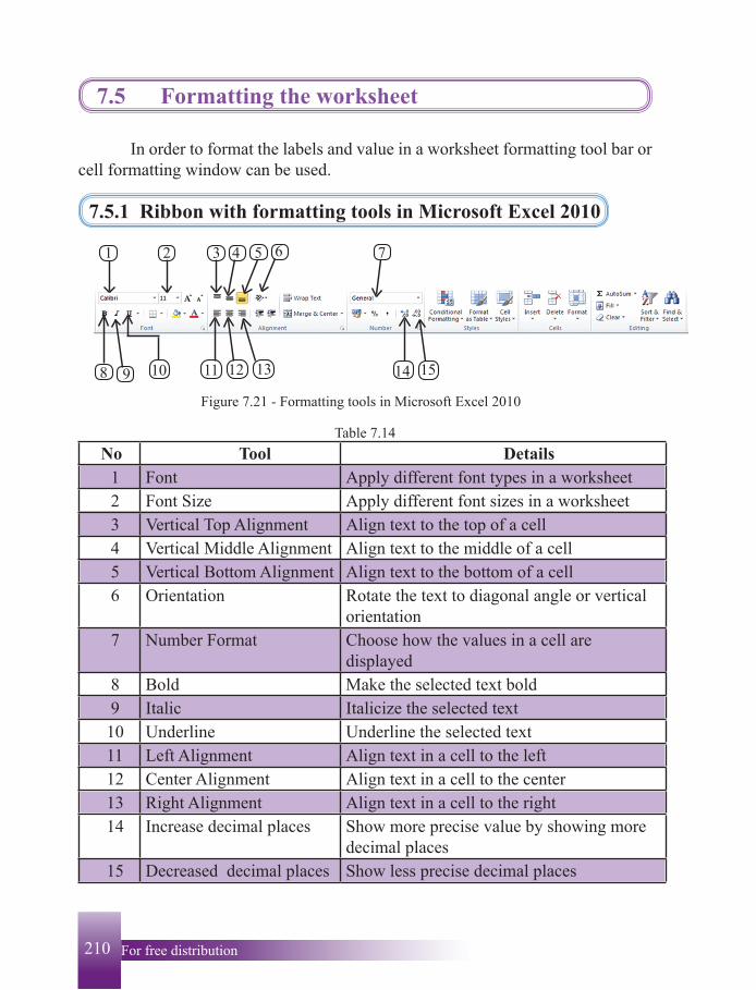
7.5.1 Ribbon with formatting tools in Microsoft Excel 2010
Table 7.14 No Tool Details
1 Font Apply different font types in a worksheet 2 Font Size Apply different font sizes in a worksheet 3 Vertical Top Alignment Align text to the top of a cell 4 Vertical Middle Alignment Align text to the middle of a cell 5 Vertical Bottom Alignment Align text to the bottom of a cell 6 Orientation Rotate the text to diagonal angle or vertical
orientation 7 Number Format Choose how the values in a cell are
displayed 8 Bold Make the selected text bold 9 Italic Italicize the selected text 10 Underline Underline the selected text 11 Left Alignment Align text in a cell to the left 12 Center Alignment Align text in a cell to the center 13 Right Alignment Align text in a cell to the right 14 Increase decimal places Show more precise value by showing more
decimal places 15 Decreased decimal places Show less precise decimal places
21 3
1310 11 151412
5 6
9
7
8
4
Figure 7.21 - Formatting tools in Microsoft Excel 2010
211 For free distributionFor free distribution210
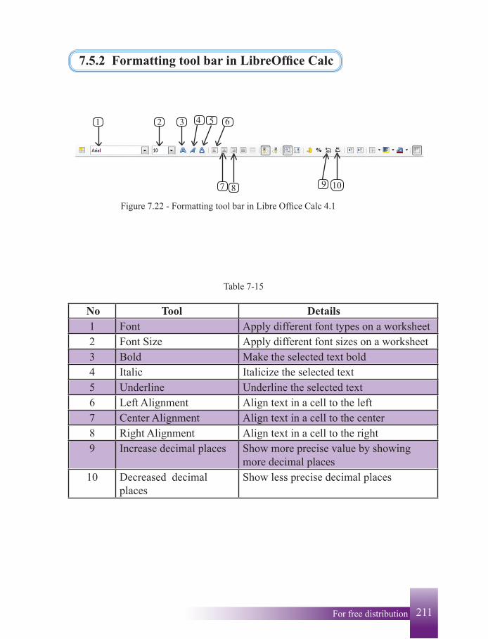
7.5.2 Formatting tool bar in LibreOffice Calc
8
3 4 5 61 2
7 9 10
Figure 7.22 - Formatting tool bar in Libre Office Calc 4.1
Table 7-15
No Tool Details1 Font Apply different font types on a worksheet2 Font Size Apply different font sizes on a worksheet3 Bold Make the selected text bold4 Italic Italicize the selected text5 Underline Underline the selected text6 Left Alignment Align text in a cell to the left 7 Center Alignment Align text in a cell to the center8 Right Alignment Align text in a cell to the right9 Increase decimal places Show more precise value by showing
more decimal places10 Decreased decimal
placesShow less precise decimal places
213 For free distributionFor free distribution212
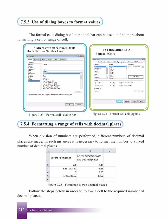
7.5.3 Use of dialog boxes to format values
The formal cells dialog box’ in the tool bar can be used to find more about formatting a cell or range of cell.
Figure 7.23 - Format cells dialog box Figure 7.24 - Format cells dialog box
In Microsoft Office Excel 2010 Home Tab → Number Group In LibreOffice Calc
Format→Cells
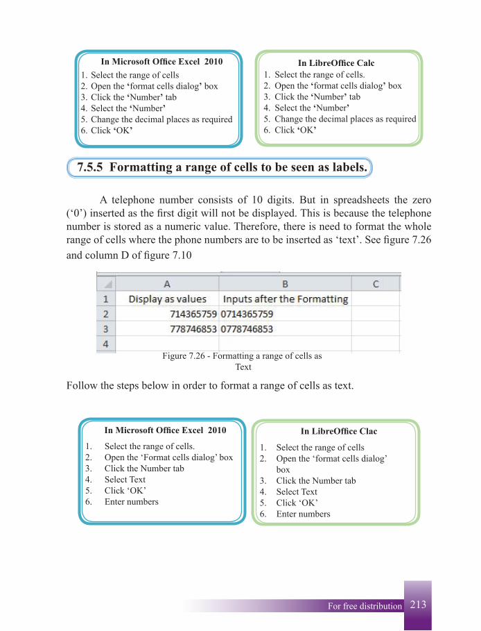
7.5.4 Formatting a range of cells with decimal places
When division of numbers are performed, different numbers of decimal places are made. In such instances it is necessary to format the number to a fixed number of decimal places.
Figure 7.25 - Formatted to two decimal places
Follow the steps below in order to follow a cell to the required number of decimal places.
213 For free distributionFor free distribution212
In Microsoft Office Excel 20101. Select the range of cells2. Open the ‘format cells dialog’ box3. Click the ‘Number’ tab4. Select the ‘Number’ 5. Change the decimal places as required6. Click ‘OK’
In LibreOffice Calc1. Select the range of cells. 2. Open the ‘format cells dialog’ box3. Click the ‘Number’ tab4. Select the ‘Number’5. Change the decimal places as required6. Click ‘OK’
7.5.5 Formatting a range of cells to be seen as labels.
A telephone number consists of 10 digits. But in spreadsheets the zero (‘0’) inserted as the first digit will not be displayed. This is because the telephone number is stored as a numeric value. Therefore, there is need to format the whole range of cells where the phone numbers are to be inserted as ‘text’. See figure 7.26 and column D of figure 7.10
Figure 7.26 - Formatting a range of cells as Text
Follow the steps below in order to format a range of cells as text.
In Microsoft Office Excel 2010
1. Select the range of cells.2. Open the ‘Format cells dialog’ box3. Click the Number tab4. Select Text 5. Click ‘OK’ 6. Enter numbers
In LibreOffice Clac
1. Select the range of cells 2. Open the ‘format cells dialog’
box3. Click the Number tab4. Select Text 5. Click ‘OK’ 6. Enter numbers
215 For free distributionFor free distribution214
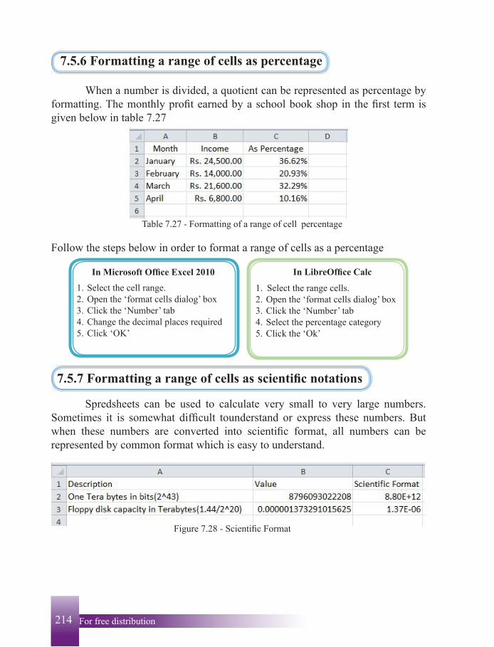
7.5.6 Formatting a range of cells as percentage
When a number is divided, a quotient can be represented as percentage by formatting. The monthly profit earned by a school book shop in the first term is given below in table 7.27
Table 7.27 - Formatting of a range of cell percentage
Follow the steps below in order to format a range of cells as a percentage
In Microsoft Office Excel 2010 1. Select the cell range.2. Open the ‘format cells dialog’ box3. Click the ‘Number’ tab4. Change the decimal places required5. Click ‘OK’
In LibreOffice Calc
1. Select the range cells.2. Open the ‘format cells dialog’ box3. Click the ‘Number’ tab4. Select the percentage category5. Click the ‘Ok’
7.5.7 Formatting a range of cells as scientific notations
Spredsheets can be used to calculate very small to very large numbers. Sometimes it is somewhat difficult tounderstand or express these numbers. But when these numbers are converted into scientific format, all numbers can be represented by common format which is easy to understand.
Figure 7.28 - Scientific Format
215 For free distributionFor free distribution214
Follow the steps below in order to format a range of cells as a percentage
In Libre Office Celc1. Select the range of cells2. Open the format cells dialog box3. Click the ‘Number’ tab4. Select ‘Scientific’ 5. Change the decimal places as needed6. Cilick ‘OK’
In Microsoft Office Excel 20101. Select the cell range.2. Open the ‘format cells dialog’ box3. Click the ‘Number’ tab4. Select ‘Scientific’ 5. Change the decimal places as
needed6. Click ‘OK’
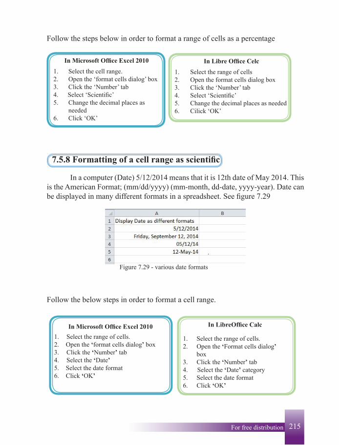
7.5.8 Formatting of a cell range as scientific
In a computer (Date) 5/12/2014 means that it is 12th date of May 2014. This is the American Format; (mm/dd/yyyy) (mm-month, dd-date, yyyy-year). Date can be displayed in many different formats in a spreadsheet. See figure 7.29
Figure 7.29 - various date formats
Follow the below steps in order to format a cell range.
In Microsoft Office Excel 2010 1. Select the range of cells. 2. Open the ‘format cells dialog’ box3. Click the ‘Number’ tab4. Select the ‘Date’ 5. Select the date format6. Click ‘OK’
In LibreOffice Calc
1. Select the range of cells. 2. Open the ‘Format cells dialog’
box3. Click the ‘Number’ tab4. Select the ‘Date’ category5. Select the date format6. Click ‘OK’
217 For free distributionFor free distribution216
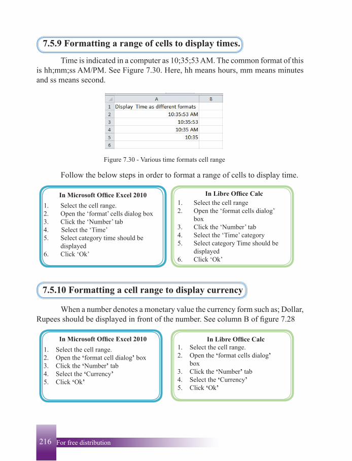
7.5.9 Formatting a range of cells to display times.
Time is indicated in a computer as 10;35;53 AM. The common format of this is hh;mm;ss AM/PM. See Figure 7.30. Here, hh means hours, mm means minutes and ss means second.
Figure 7.30 - Various time formats cell range
Follow the below steps in order to format a range of cells to display time.
In Microsoft Office Excel 20101. Select the cell range.2. Open the ‘format’ cells dialog box3. Click the ‘Number’ tab4. Select the ‘Time’5. Select category time should be
displayed6. Click ‘Ok’
In Libre Office Calc1. Select the cell range2. Open the ‘format cells dialog’
box3. Click the ‘Number’ tab4. Select the ‘Time’ category5. Select category Time should be
displayed6. Click ‘Ok’
7.5.10 Formatting a cell range to display currency
When a number denotes a monetary value the currency form such as; Dollar, Rupees should be displayed in front of the number. See column B of figure 7.28
In Microsoft Office Excel 20101. Select the cell range.2. Open the ‘format cell dialog’ box3. Click the ‘Number’ tab4. Select the ‘Currency’ 5. Click ‘Ok’
In Libre Office Calc1. Select the cell range.2. Open the ‘format cells dialog’
box3. Click the ‘Number’ tab4. Select the ‘Currency’5. Click ‘Ok’
217 For free distributionFor free distribution216
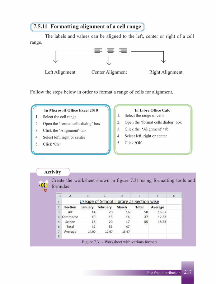
7.5.11 Formatting alignment of a cell range The labels and values can be aligned to the left, center or right of a cell range.
Left Alignment Center Alignment Right Alignment
Follow the steps below in order to format a range of cells for alignment.
In Microsoft Office Excel 20101. Select the cell range
2. Open the ‘format cells dialog’ box
3. Click the ‘Alignment’ tab
4. Select left, right or center
5. Click ‘Ok’
In Libre Office Calc1. Select the range of cells
2. Open the ‘format cells dialog’ box
3. Click the ‘Alignment’ tab
4. Select left, right or center
5. Click ‘Ok’
Activity
Create the worksheet shown in figure 7.31 using formatting tools and formulae.
Figure 7.31 - Worksheet with various formats
219 For free distributionFor free distribution218
1. Center align column A and row 22. Make row 2 Bold3. Underline the heading in row. Make the font size 164. Italicize cells A3, A4, A5 5. Use function SUM and write a formula in B7 to calculate the total
for the month of January.6. Use function AVERAGE and write a formula in B7 to calculate the average for
the month of January.7. Copy the formulae in B6 and B7 and use them to calculate the total and average
for other remaining months.8. Use SUM function to get total of Arts Section in the cell E3.9. Use AVERAGE function to get average of Arts section in the cell F3.10. Copy the formulae in E3 and F3 and use them to calculate the total and average
for other remaining departments.
7.6 Relative and absolute cell reference
7.6.1 Copying a formula
A class teacher to calculates the total and average of each student after the examinations of a term. However, using an electronic spreadsheet would make this task efficient. This is because one can copy the formulae once apply it to many other instances. Hence let us look at the steps on how to copy formulae along rows and columns.
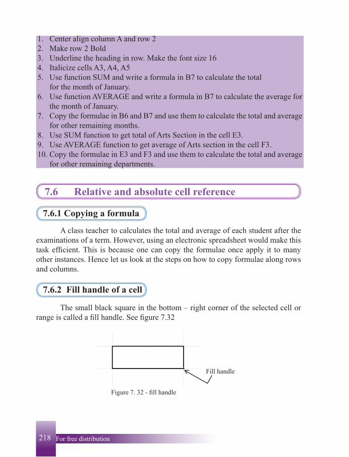
7.6.2 Fill handle of a cell
The small black square in the bottom – right corner of the selected cell or range is called a fill handle. See figure 7.32
Figure 7. 32 - fill handle
Fill handle
219 For free distributionFor free distribution218
7.6.3 Use of fill handle for copying formulae
Follow the steps below to copy formulae using the fill handle.1. Select the cell which contains the formula2. Click the small black square in the bottom-right corner of the selected cell 3. Drag the fill handle up to the required cell
7.6.4 Use of copy and paste commands for copying formulae
Follow the following steps to copy formulae using the copy – paste commands which contains the formula
(1) Select the cell(2) Copy the contents of the selected cell (Ctrl+C)(3) Select the cell to which the formula is to be pasted(4) Paste the contents on the selected cell (Ctrl+V)
7.6.5 Relative and absolute cell reference
A cell address (reference) consists of a column letter and a row number. In a formula such a cell address is always called as a relative reference. The dollar sign ($) when sign is placed befor a row number absolute row is obtained, when ($) mark is placed before a column name an absolute column is obtained, when ($) is placed before column name and row uumber absolute column and row absolure can be obtainedExample
H2 - Relative cell referenceH$2 - Row absolute cell reference$H2 - Column absolute cell reference$H$2 - Row and column absolute cell reference
7.6.6 Relative cell reference
If the row number and the column letter of the adjacent cells change accordingly when a formula is copied, such cell addresses are called relative cell reference.
221 For free distributionFor free distribution220
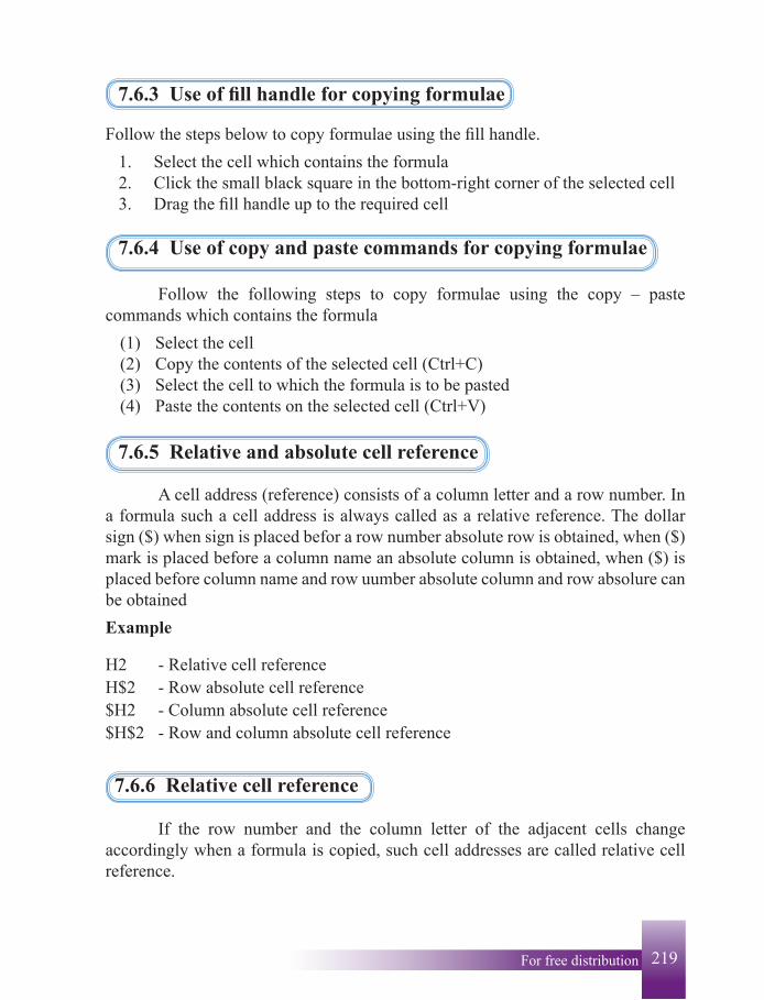
ExampleWhen the formula A1+B1 entered in C1 is dragged down along column C and dragged sideways along row 1, the cell references change accordingly as shown in image 7.33 below. Hence the cell references A1 and B1 could be considered relative cell reference.
Figure 7'33 - worksheet with reletive cell reference
Column letters change
Row numbers change
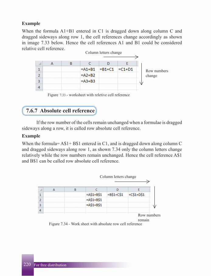
7.6.7 Absolute cell reference
If the row number of the cells remain unchanged when a formulae is dragged sideways along a row, it is called row absolute cell reference.ExampleWhen the formula= A$1+ B$1 entered in C1, and is dragged down along column C and dragged sideways along row 1, as shown 7.34 only the column letters change relatively while the row numbers remain unchanged. Hence the cell reference A$1 and B$1 can be called row absolute cell reference.
Column letters change
Row numbers remain
Figure 7.34 - Work sheet with absolute row cell reference
221 For free distributionFor free distribution220
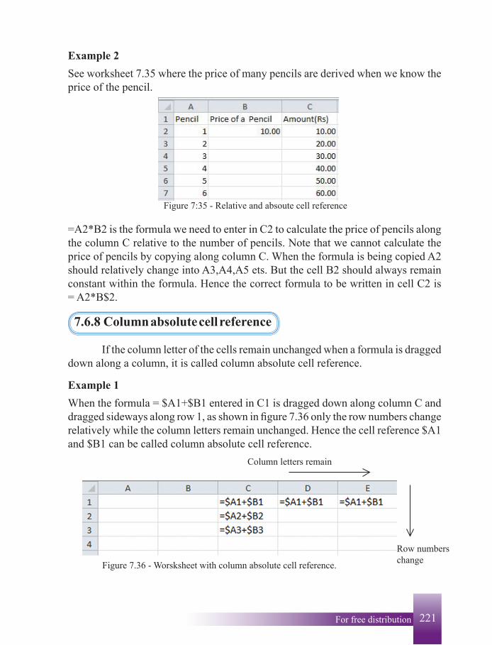
Example 2See worksheet 7.35 where the price of many pencils are derived when we know the price of the pencil.
Figure 7:35 - Relative and absoute cell reference
=A2*B2 is the formula we need to enter in C2 to calculate the price of pencils along the column C relative to the number of pencils. Note that we cannot calculate the price of pencils by copying along column C. When the formula is being copied A2 should relatively change into A3,A4,A5 ets. But the cell B2 should always remain constant within the formula. Hence the correct formula to be written in cell C2 is = A2*B$2.
7.6.8 Column absolute cell reference
If the column letter of the cells remain unchanged when a formula is dragged down along a column, it is called column absolute cell reference.
Example 1 When the formula = $A1+$B1 entered in C1 is dragged down along column C and dragged sideways along row 1, as shown in figure 7.36 only the row numbers change relatively while the column letters remain unchanged. Hence the cell reference $A1 and $B1 can be called column absolute cell reference.
Column letters remain
Row numbers change Figure 7.36 - Worsksheet with column absolute cell reference.
223 For free distributionFor free distribution222
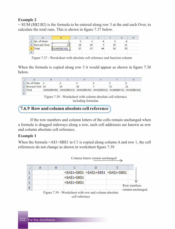
Example 2= SUM ($B2:B2) is the formula to be entered along row 3 at the end each Over, to calculate the total runs. This is shown in figure 7.37 below.
Figure 7.37 - Worsksheet with absolute cell reference and function column
When the formula is copied along row 3 it would appear as shown in figure 7.38 below.
Figure 7.38 - Worsksheet with column absolute cell reference including formulae
7.6.9 Row and column absolute cell reference
If the row numbers and column letters of the cells remain unchanged when a formula is dragged sideways along a row, such cell addresses are known as row and column absolute cell reference.Example 1When the formula =A$1+$B$1 in C1 is copied along column A and row 1, the cell references do not change as shown in worksheet figure 7.39
Column letters remain unchanged
Row numbers remain unchanged.
Figure 7.39 - Worsksheet with row and column absolute cell reference
223 For free distributionFor free distribution222
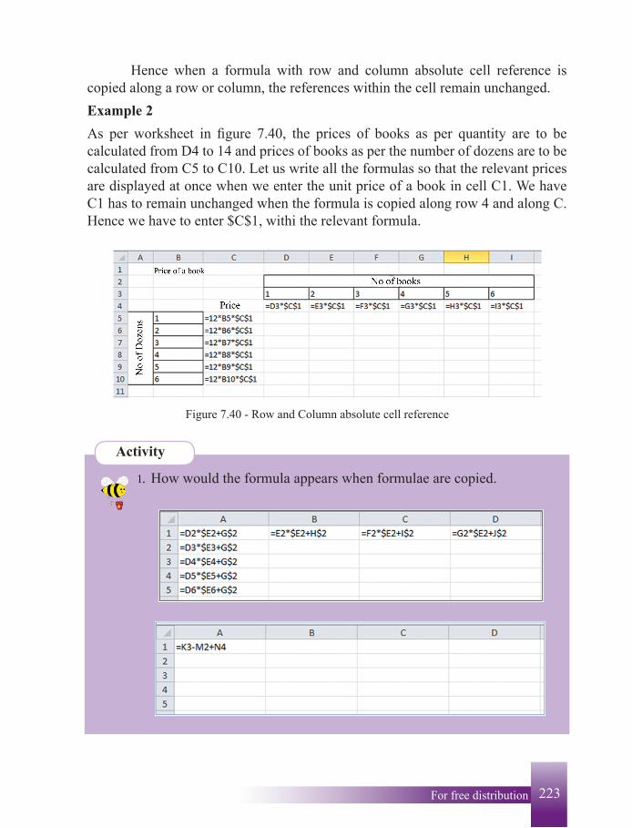
Hence when a formula with row and column absolute cell reference is copied along a row or column, the references within the cell remain unchanged.Example 2As per worksheet in figure 7.40, the prices of books as per quantity are to be calculated from D4 to 14 and prices of books as per the number of dozens are to be calculated from C5 to C10. Let us write all the formulas so that the relevant prices are displayed at once when we enter the unit price of a book in cell C1. We have C1 has to remain unchanged when the formula is copied along row 4 and along C. Hence we have to enter $C$1, withi the relevant formula.
Figure 7.40 - Row and Column absolute cell reference
Activity
1' How would the formula appears when formulae are copied.
225 For free distributionFor free distribution224
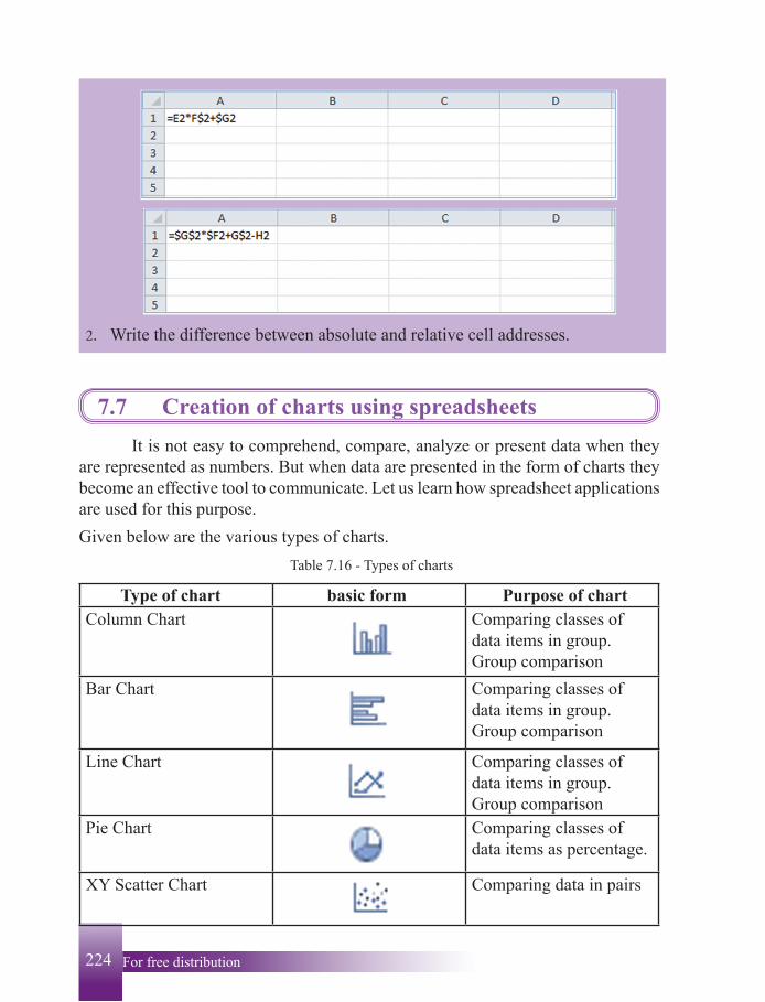
2' Write the difference between absolute and relative cell addresses.
7.7 Creation of charts using spreadsheets It is not easy to comprehend, compare, analyze or present data when they are represented as numbers. But when data are presented in the form of charts they become an effective tool to communicate. Let us learn how spreadsheet applications are used for this purpose.Given below are the various types of charts. Table 7.16 - Types of charts
Type of chart basic form Purpose of chartColumn Chart Comparing classes of
data items in group.Group comparison
Bar Chart Comparing classes of data items in group.Group comparison
Line Chart Comparing classes of data items in group.Group comparison
Pie Chart Comparing classes of data items as percentage.
XY Scatter Chart Comparing data in pairs
225 For free distributionFor free distribution224
Activity
Write down two examples use for the chart types in Figure 7.15.
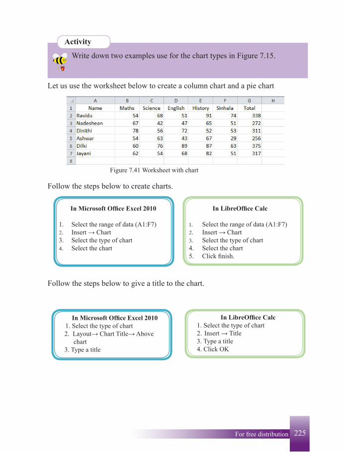
Let us use the worksheet below to create a column chart and a pie chart
Figure 7.41 Worksheet with chart
Follow the steps below to create charts.
In Microsoft Office Excel 2010
1. Select the range of data (A1:F7)2' Insert → Chart3. Select the type of chart4' Select the chart
In LibreOffice Calc
1' Select the range of data (A1:F7)2' Insert → Chart3' Select the type of chart4. Select the chart5. Click finish.
Follow the steps below to give a title to the chart.
In Microsoft Office Excel 2010 1. Select the type of chart 2. Layout→ Chart Title→ Above chart 3. Type a title
In LibreOffice Calc1. Select the type of chart2. Insert → Title3. Type a title4. Click OK
227 For free distributionFor free distribution226
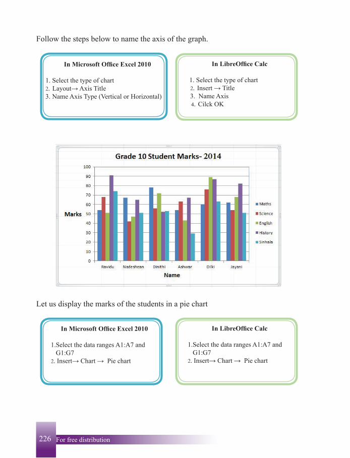
Follow the steps below to name the axis of the graph.
In Microsoft Office Excel 2010
1. Select the type of chart2' Layout→ Axis Title3. Name Axis Type (Vertical or Horizontal)
In LibreOffice Calc
1. Select the type of chart 2' Insert → Title 3. Name Axis 4' Cilck OK
Let us display the marks of the students in a pie chart
In Microsoft Office Excel 2010
1.Select the data ranges A1:A7 and G1:G72' Insert→ Chart → Pie chart
In LibreOffice Calc
1.Select the data ranges A1:A7 and G1:G72' Insert→ Chart → Pie chart
227 For free distributionFor free distribution226
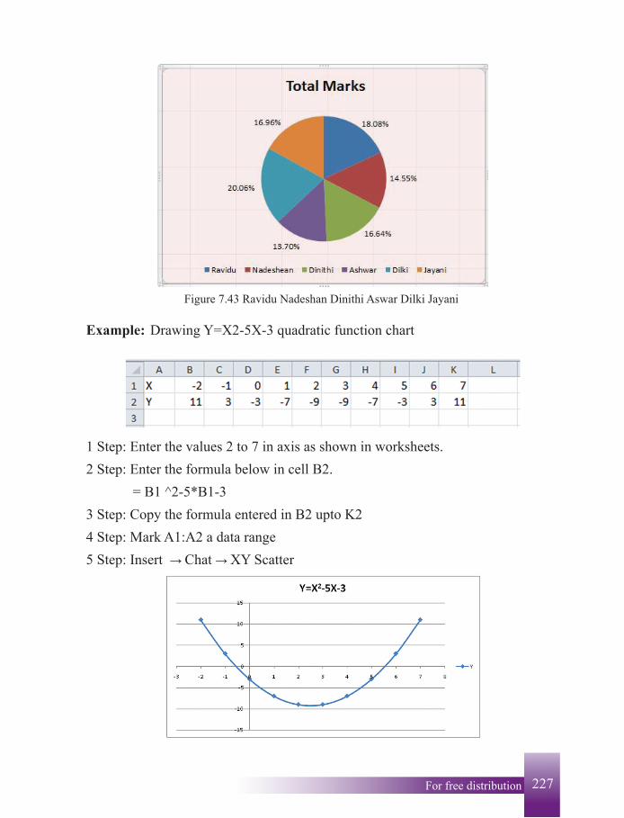
Figure 7.43 Ravidu Nadeshan Dinithi Aswar Dilki Jayani
Example: Drawing Y=X2-5X-3 quadratic function chart
1 Step: Enter the values 2 to 7 in axis as shown in worksheets.2 Step: Enter the formula below in cell B2. = B1 ^2-5*B1-33 Step: Copy the formula entered in B2 upto K24 Step: Mark A1:A2 a data range5 Step: Insert → Chat → XY Scatter

229 For free distributionFor free distribution228
Exercise 1) Provide answers based on the worksheet below.
Figure 7.44
(1) Name the cell range where 2,6,10,14 are present.(2) Name the cell range where 9,10,11,12 are present.(3) Name the cell range where 6,7,8,10,11,12 are present.(4) Write the formula in A5 using only cell addresses to calculate the total of the values from A1 to A4.(5) Write the formula in A3 using function to calculate the total of the values from A3 to D3.(6) Write how you would copy the formula in E3 to E4 (7) Write the formula in A5 using function to calculate the average of the values from A3 to D3.
Activity
Create the below worksheet using a spreadsheet. Those who were absent are marked 'ab'.
Figure 7-45 Marks List
229 For free distributionFor free distribution228
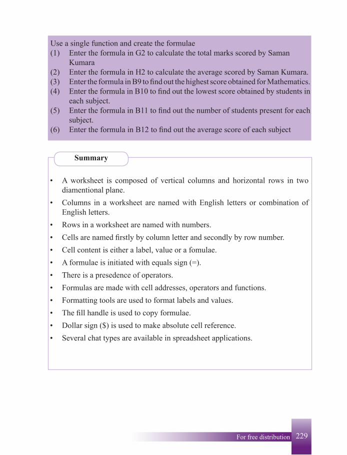
Use a single function and create the formulae (1) Enter the formula in G2 to calculate the total marks scored by Saman
Kumara(2) Enter the formula in H2 to calculate the average scored by Saman Kumara. (3) Enter the formula in B9 to find out the highest score obtained for Mathematics. (4) Enter the formula in B10 to find out the lowest score obtained by students in
each subject.(5) Enter the formula in B11 to find out the number of students present for each
subject.(6) Enter the formula in B12 to find out the average score of each subject
• A worksheet is composed of vertical columns and horizontal rows in two diamentional plane.
• Columns in a worksheet are named with English letters or combination of English letters.
• Rows in a worksheet are named with numbers. • Cells are named firstly by column letter and secondly by row number. • Cell content is either a label, value or a fomulae. • A formulae is initiated with equals sign (=). • There is a presedence of operators. • Formulas are made with cell addresses, operators and functions. • Formatting tools are used to format labels and values. • The fill handle is used to copy formulae. • Dollar sign ($) is used to make absolute cell reference. • Several chat types are available in spreadsheet applications.
Summary
Top Related