


Languages
Pages
Legal


BIOMASS TO ETHANOL: PROCESS SIMULATION,
VALIDATION AND SENSITIVITY ANALYSIS OF
A GASIFIER AND A BIOREACTOR
By
SIRIGUDI RAHUL RAO
Bachelor of Engineering
National Institute of Technology Karnataka, India
2002
Submitted to the Faculty of the Graduate College of the
Oklahoma State University in partial fulfillment of
the requirements for the Degree of
MASTER OF SCIENCE December, 2005

BIOMASS TO ETHANOL: PROCESS SIMULATION,
VALIDATION AND SENSITIVITY ANALYSIS OF
A GASIFIER AND A BIOREACTOR
Thesis Approved:
Arland H. Johannes
Thesis Adviser
Karen High
Sundar Madihally
A. Gordon Emslie
Dean of the Graduate College
ii

ACKNOWLEDGEMENTS
I would like to acknowledge S. Ramakrishna and S. Vijayalakshmi, the two people who
have always stood by me, encouraging me since my first footsteps. I have been truly
inspired by my parents while taking most of my bolder steps and I thank them for all the
sacrifices they have made for me. I am thankful to my Late grandfather S.
Chandrashekhar for always reminding me not to lose faith in myself. I will always
remember my aunt Asha for the wonderful woman that she is. I dedicate this work to my
family.
I would like to thank my adviser, Dr. A. H. Johannes for his guidance throughout my
research. A gem of a man that I have found in my adviser, is more than any graduate
student deserves. His direction was always gentle and encouraging, for which I am truly
grateful. It has been an honor working with him. I am grateful to Dr. AJ and Dr. Randy
Lewis for bringing this project to the Department of Chemical Engineering and allowing
me the opportunity to work on the project. I would also like to thank Dr. Karen High and
Dr. Sundar Madihally for their support and interest in my research. I would also like to
thank Dr. Khaled Gasem for his comments and interest in my research. I thank my
friends at the Department of Chemical Engineering, Shirley, Carolyn and Sam who were
repeatedly bugged by me during my stay. Genny, I salute your patience. Eileen, you are
one of the sweetest persons I have ever come across.
iii

I thank my friend and colleague, Aniket Patankar for his love and support. I thank my
friends Arun, Konda, Vijay, Pranay, Venkat, Priya and Makarand for making my stay in
Stillwater a lot of fun. I am grateful to Vidya for her love, care and support during my
masters. Thank you for being what you are.
I thank Asma for providing me with experimental data on the bioreactor and valuable
inputs on my work. I also thank Bruno and Biosystems Engineering for providing me
with experimental data on the gasifier.
Finally, I would like to thank all the sponsors of this research project in the Department
of Agriculture and the School of Chemical Engineering at Oklahoma State University.
iv

TABLE OF CONTENTS Chapter Page 1. BIOMASS FERMENTATION TO ETHANOL: AN OVERVIEW ..............................1
1.1 Introduction........................................................................................................1 1.2 Renewable Source of Energy supply .................................................................4 1.3 Reduction/elimination of MTBE .......................................................................4 1.4 Environmental Benefits and Climatic change....................................................7 1.5 Less International Dependence ..........................................................................8 1.6 Economic Benefits .............................................................................................9 1.7 Disadvantages of Ethanol as a Fuel ...................................................................9 1.8 Ethanol Manufacturing Processes....................................................................10
1.8.1 Ethanol Production from Corn..........................................................10 1.8.2 Ethanol Production from Lignocellulosic Feedstock........................11 1.8.3 Ethanol Production from the Gasification and Fermentation Process ..............................................................................................11
1.9 Purpose of the Study ........................................................................................12
2. GASIFICATION, FERMENTATION AND PROCESS SIMULATION: LITERATURE REVIEW ......................................................................................14
2.1 Gasification ......................................................................................................14
2.1.1 Gasifier Pilot Plant Set-up ...............................................................16 2.2 Syngas Fermentation........................................................................................20
2.2.1 Bioreactor Laboratory Scale Set-up.................................................21 2.3 Process Simulation...........................................................................................24 2.3.1 Biomass Gasification Modeling and Simulation .............................27
2.3.2 Syngas Fermentation Modeling and Simulation..............................28
3. DEVELOPMENT OF PROCESS MODELS IN ASPEN PLUS .................................31
3.1 Process Characterization..................................................................................31 3.2 Component Specification.................................................................................32 3.3 Physical Property Estimation...........................................................................32 3.4 Built-In Reactor Models in Aspen Plus ...........................................................33 3.5 Process Flowsheet Development .....................................................................33 3.6 Process Variables Specification.......................................................................35 3.7 Sensitivity Analysis Tools ...............................................................................35 3.8 Simulation Output Data ...................................................................................35
v

Chapter Page 4. MODELING OF A GASIFIER AND A BIOREACTOR ............................................37
4.1 Modeling a Gasifier as a Gibbs Reactor Model...............................................37 4.1.1 Base Case Simulation ......................................................................38 4.1.2 Fuel Sensitivity Analysis .................................................................38 4.1.3 Moisture Sensitivity Analysis ..........................................................39 4.1.4 Temperature Sensitivity Analysis ....................................................39 4.1.5 Air Fuel Ratio Sensitivity Analysis .................................................39 4.1.6 Equivalence Ratio Sensitivity Analysis ...........................................40
4.2 Bioreactor Modeling in a Gibbs Reactor Model..............................................41 4.2.1 Base Case Simulation ......................................................................42 4.2.2 Carbon Monoxide Sensitivity Analysis ...........................................42 4.2.3 Carbon Dioxide Sensitivity Analysis...............................................43 4.2.4 Hydrogen Sensitivity Analysis ........................................................44 4.2.5 Media Sensitivity Analysis ..............................................................44
4.3 Bioreactor Modeling in a Stoichiometric Reactor Model................................45 4.3.1 Base Case Simulation ......................................................................46 4.3.2 Sensitivity of the Model to Stoichiometric Conversions .................47
5. RESULTS AND DISCUSSION...................................................................................49
5.1 Gasifier Modeling ............................................................................................49 5.1.1 Base Case Simulation Output and Model Validation ......................49 5.1.2 Effect of Fuel Variation on Production of Syngas...........................54 5.1.3 Effect of Moisture Variation on Production of Syngas ...................55 5.1.4 Effect of Temperature Variation on Syngas Production..................57 5.1.5 Effect of Air Fuel Ratio on Syngas Production ...............................61 5.1.6 Effect of Variation of Equivalence Ratio on Syngas Production ....63 5.1.7 Energy Balance for the Gasifier Model ...........................................67
5.2 Bioreactor Modeling ........................................................................................67 5.2.1 Base Case Simulation Output and Model Validation: Gibbs
Reactor .............................................................................................68 5.2.2 Effect of Variation of Carbon Monoxide on Ethanol Production....71 5.2.3 Effect of Variation of Carbon Dioxide on Ethanol Production .......72 5.2.4 Effect of Variation of Hydrogen on Ethanol Production .................73 5.2.5 Effect of Variation of Media on Ethanol Production.......................75 5.2.6 Presence of Methane in the Model...................................................76 5.2.7 Base Case Simulation Output and Model Validation: Stoichiometric Reactor .............................................................................................77 5.2.8 Effect of Stoichiometric Conversion on Ethanol Production ...........81 5.2.9 Energy Balance for the Bioreactor Model ........................................84
6. CONCLUSIONS AND RECOMMENDATIONS .......................................................85
vi

Chapter Page 6.1 Conclusions......................................................................................................85
6.1.1 Gasifier simulation............................................................................85 6.1.2 Bioreactor simulation........................................................................87
6.2 Recommendations for future work ..................................................................89
REFERENCES ..................................................................................................................91
APPENDIXES ...................................................................................................................96
APPENDIX A: Simulation Data Tables ................................................................96 APPENDIX B: Aspen PlusTM Output Files .........................................................125
vii

LIST OF TABLES
Table Page 1.1 Estimated U.S consumption of Fuel Ethanol, MTBE and Gasoline..............................4
1.2 State MTBE bans ...........................................................................................................6
5.1 Experimental input composition of feed streams to gasifier .......................................50
5.2 Comparison of simulation and experimental data .......................................................52
5.3 Experimental input data to the bioreactor....................................................................68
5.4 Comparison of simulation and experimental data: Gibbs reactor model.....................69
5.5 Comparison of simulation and experimental data: Stoichiometric reactor model.......79
viii

LIST OF FIGURES
Figure Page
1.1 Historic U.S fuel ethanol production .............................................................................3
2.1 Gasifier pilot plant set up.............................................................................................18
2.2 Gasifier pilot plant flowsheet.......................................................................................19
2.3 Bioreactor lab scale set up flowsheet...........................................................................23
2.4 Simulation model development algorithm...................................................................25
3.1 Flowsheet of the bioreactor simulation using a stoichiometric reactor model in Aspen
PlusTM...........................................................................................................................34
3.2 Snapshot of a typical specifications input form in Aspen PlusTM................................36
4.1 A snapshot of a typical reaction stoichiometry input form in a stoichiometric reactor
model developed in Aspen PlusTM...............................................................................48
5.1 Graphical comparison of simulation data with experimental results...........................53
5.2 Effect of variation in the biomass feed rate on the exhaust gas composition ..............55
5.3 Effect of variation in the moisture associated with biomass feed rate on the exhaust
gas composition ...........................................................................................................56
5.4 Effect of variation in the operation temperature on the exhaust gas composition: mass
basis..............................................................................................................................58
5.5 Effect of variation in the operation temperature on the exhaust gas composition: mole
basis..............................................................................................................................59
ix

5.6 Effect of variation in the operation temperature on the hydrocarbons in the exhaust
gas ................................................................................................................................60
5.7 Effect of variation in the Air – Fuel Ratio on the exhaust gas composition:
mass basis.....................................................................................................................61
5.8 Effect of variation in the Air – Fuel Ratio on the exhaust gas composition:
mole basis.....................................................................................................................63
5.9 Effect of variation in the Equivalence Ratio on the exhaust gas composition.............64
5.10 Effect of variation in the Air – Fuel Ratio on the production of CO and CO2 at other
temperatures..............................................................................................................66
5.11 Effect of variation in the Air – Fuel Ratio on the production of H2 and N2 at other
temperatures..............................................................................................................67
5.12 Effect of the variation in CO levels in feed gas on the ethanol produced .................72
5.13 Effect of the variation in CO2 levels in feed gas on the ethanol produced ................73
5.14 Effect of the variation in H2 levels in feed gas on the ethanol produced...................74
5.15 Effect of the variation in the media feed on the ethanol produced ............................76
5.16 Effect of variation in the stoichiometric conversions on the exit gas composition ...78
5.17 Graphical comparison of simulation data with experimental results.........................80
5.18 Effect of variation in the stoichiometric conversion (E1) on the exit gas
composition...............................................................................................................82
5.19 Effect of variation in the stoichiometric conversion (E2) on the exit gas
composition...............................................................................................................83
5.20 Effect of variation in the stoichiometric conversions on the ethanol produced.........84
x

NOMENCLATURE
atm Atmosphere
AF Air Fuel (ratio)
bar bars
Btu British thermal units
C carbon
°C degree centigrade
CAA Clean Air Act
cc/min cubic centimeter per minute
CH4 methane
C2H2 acetylene
C2H4 ethylene
C2H5OH ethanol
CO carbon monoxide
CO2 carbon dioxide
CSTR continuous stirred tank reactor
DOE Department of Energy
E stoichiometric conversion
EOS equation of state
EPA Environmental Protection Agency
xi
ER Equivalence Ratio
FBN fuel bound nitrogen
GHG green house gases
H2 hydrogen
H2O water
HNO3 nitric acid
K kelvin
Kg/hr kilogram per hour
Kg/sec kilogram per second
KJ/mol kilo joule per mole
Kmol kilo mole
mol mole
mol frac mole fraction
MTBE methyl tertiary butyl ether
NH3 ammonia
NOx nitrogen oxide (x is 1, 2 or 3)
N2O nitrous oxide
NRTL Non Random Two Liquid
O2 oxygen
psi pounds per square inch
P7T strain identification of C. carboxidivorans species
RFG reformulated gasoline
RFS Renewable Fuel Standard
xii

VOC volatile organic compounds
vol % percentage by volume
wt % percentage by weight
xiii

CHAPTER 1
BIOMASS FERMENTATION TO ETHANOL: AN OVERVIEW 1.1 Introduction
Since the 1973-1974 oil embargo, the requirement to conserve petroleum
resources has become imminent and new processes for the development of alternate fuels
are being investigated (Paul, 1979). The transportation sector with its nearly total
dependence on petroleum has virtually no capacity to switch to other fuels in the event of
a supply disruption (Lynd et al., 1991). In light of the rapid changes in the regulatory and
legislative aspects of government in the past two decades, ethanol has taken an important
role in bringing together often conflicting environmental and security concerns
(Yacobucci and Womach, 2004).
Production of ethanol from biomass has increasingly gained importance since the
supply of biomass from agriculture is readily available in the United States. In 2003,
99% of fuel ethanol consumed in the United States was in the form of “gasohol” or “E
10” which are blends of gasoline with up to 10% of ethanol (Yacobucci and Womach,
2004). Environmental issues limiting the increase of CO2 in the atmosphere and global
warming due to burning of petroleum based fuels also argue for increased utilization of
ethanol. Use of alternative energy sources instead of petroleum would aid in stabilizing
the concentration of CO2 in the atmosphere (Hohenstein and Wright, 1994). The use of
fuel ethanol has been stimulated by the Clean Air Act Amendments of 1990, which
1
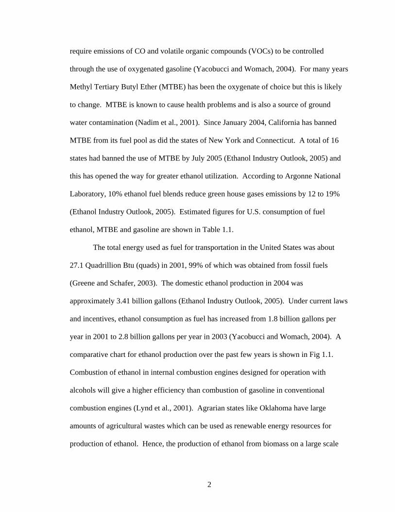
require emissions of CO and volatile organic compounds (VOCs) to be controlled
through the use of oxygenated gasoline (Yacobucci and Womach, 2004). For many years
Methyl Tertiary Butyl Ether (MTBE) has been the oxygenate of choice but this is likely
to change. MTBE is known to cause health problems and is also a source of ground
water contamination (Nadim et al., 2001). Since January 2004, California has banned
MTBE from its fuel pool as did the states of New York and Connecticut. A total of 16
states had banned the use of MTBE by July 2005 (Ethanol Industry Outlook, 2005) and
this has opened the way for greater ethanol utilization. According to Argonne National
Laboratory, 10% ethanol fuel blends reduce green house gases emissions by 12 to 19%
(Ethanol Industry Outlook, 2005). Estimated figures for U.S. consumption of fuel
ethanol, MTBE and gasoline are shown in Table 1.1.
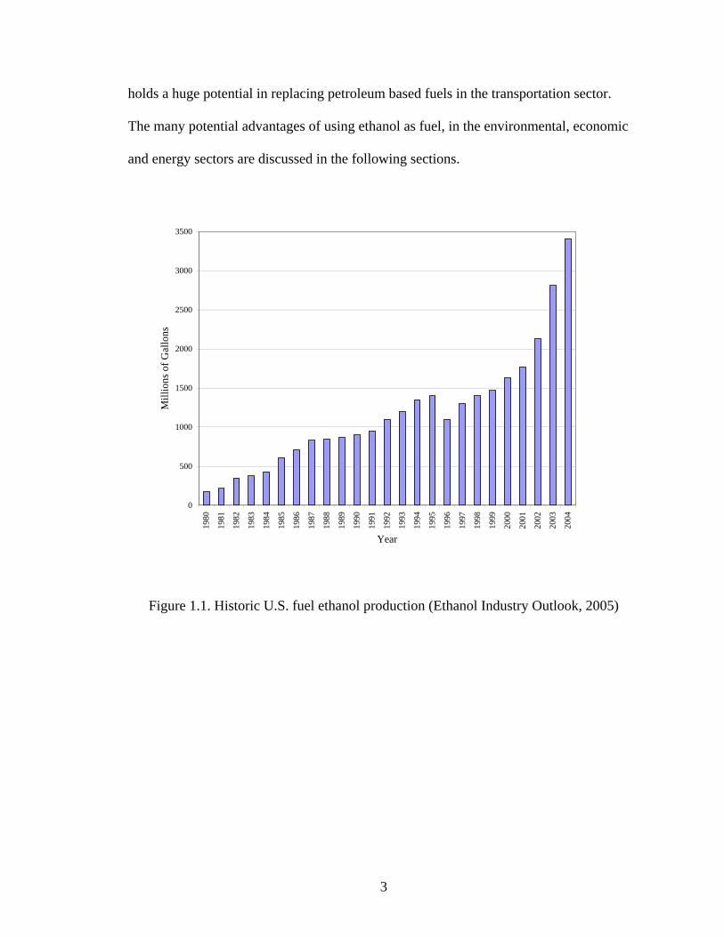
The total energy used as fuel for transportation in the United States was about
27.1 Quadrillion Btu (quads) in 2001, 99% of which was obtained from fossil fuels
(Greene and Schafer, 2003). The domestic ethanol production in 2004 was
approximately 3.41 billion gallons (Ethanol Industry Outlook, 2005). Under current laws
and incentives, ethanol consumption as fuel has increased from 1.8 billion gallons per
year in 2001 to 2.8 billion gallons per year in 2003 (Yacobucci and Womach, 2004). A
comparative chart for ethanol production over the past few years is shown in Fig 1.1.
Combustion of ethanol in internal combustion engines designed for operation with
alcohols will give a higher efficiency than combustion of gasoline in conventional
combustion engines (Lynd et al., 2001). Agrarian states like Oklahoma have large
amounts of agricultural wastes which can be used as renewable energy resources for
production of ethanol. Hence, the production of ethanol from biomass on a large scale
2
holds a huge potential in replacing petroleum based fuels in the transportation sector.
The many potential advantages of using ethanol as fuel, in the environmental, economic
and energy sectors are discussed in the following sections.
0
500
1000
1500
2000
2500
3000
3500
1980
1981
1982
1983
1984
1985
1986
1987
1988
1989
1990
1991
1992
1993
1994
1995
1996
1997
1998
1999
2000
2001
2002
2003
2004
Year
Mill
ions
of G
allo
ns
Figure 1.1. Historic U.S. fuel ethanol production (Ethanol Industry Outlook, 2005)
3

Table 1.1 Estimated U.S consumption of Fuel Ethanol, MTBE and Gasoline (Yacobucci and Womach, 2004) (thousand gasoline-equivalent gallons) 1996 1998 2000 2002E 85 694 1,727 7,704 10,075E 95 2,669 59 13 0Ethanol in Gasohol (E 10) 660,200 889,500 1,106,300 1,118,900MTBE in Gasoline 2,749,700 2,903,400 3,087,900 2,531,000Gasolinea 117,783,000 122,849,000 125,720,000 130,735,000 a Gasoline consumption includes ethanol in gasohol and MTBE in gasoline
1.2 Renewable Source of Energy supply
Biomass is the plant material derived from the reaction between CO2 and air, in
the presence of water and sunlight, via photosynthesis to produce carbohydrates that form
the building blocks of biomass (McKendry, 2002a). Agricultural biomass is abundant in
the United States; it is presently estimated to contribute on the order of 10-14% of the
worlds’ energy supply (McKendry, 2002a). Hence, fuel ethanol produced from biomass
using agricultural crop residues is a renewable source of energy.
1.3 Reduction/elimination of MTBE
The Clean Air Act Amendments of the 1990’s requires reduction in CO emissions
and VOCs through the use of oxygenated fuels (Yacobucci and Womach, 2004). While
oxygenates reduce CO and VOC emissions, they lead to higher levels of nitrogen oxides,
which are precursors to ozone formation (Yacobucci and Womach, 2004). MTBE use
4
during winter months has proven to cause significant acute health problems and illness in
large city residents (Nadim et al., 2001). MTBE moves more rapidly into groundwater
than other gasoline compounds and contaminates drinking water. MTBE is much more
resistant to biodegradation than other gasoline compounds (Nadim et al., 2001). MTBE
has also been identified as an animal carcinogen with further concern of being a human
carcinogen as well (Yacobucci and Womach, 2004). Despite the cost differential, ethanol
has many advantages over MTBE and will replace it as the gasoline additive in the future.
Ethanol contains 35% oxygen by weight which is almost twice the oxygen content of
MTBE and is a sustainable fuel; MTBE on the other hand is only produced from fossil
fuels (Yacobucci and Womach, 2004). A complete list of states where the use of MTBE
has been banned is shown in Table 1.2.
5

Table 1.2 State MTBE bans (Ethanol Industry Outlook, 2005)
State Effective Date Arizona Effective California Effective Colorado Effective Connecticut Effective Illinois Effective Indiana Effective Iowa Effective Kansas Pending federal action Kentucky 1/1/2006 Maine 1/1/2007 Michigan Effective Minnesota Effective Missouri 7/1/2005 Nebraska Effective New Hampshire Pending federal action New York Effective Ohio 7/1/2005 South Dakota Effective Washington Effective Wisconsin Effective
6

1.4 Environmental Benefits and Climatic change
Due to the requirements of the Clean Air Act (CAA) of 1990, oxygenates were
required in gasoline. Although this reduced the CO and VOC emissions to the
environment, it also increased the formation of ground level ozone. Ground level ozone
was found to be harmful to plants and causes respiratory problems in humans (Nadim et
al., 2001). As part of the CAA program, the federal government introduced the use of
reformulated gasoline (RFG) which requires the use of 2% oxygenate, met by adding
11% MTBE or 5.7% ethanol by volume. This program was intended to reduce the
emission levels of highly toxic aromatic compounds like benzene formed during the
combustion of gasoline. In conventional gasoline, aromatics which reach levels as high
as 50%, were reduced to 27% by the use of RFG (Nadim et al., 2001). The
Environmental Protection Agency (EPA) states that the usage of RFG has led to a 17%
reduction in VOCs and a 30% reduction in toxic emissions (Yacobucci and Womach,
2004).
Another environmental factor supporting the use of ethanol as an additive in
motor fuels is the emission of green house gases (GHG). Global warming has been an
important environmental concern in the past two decades. Global warming occurs when
temperatures increase due to the emission of CO2, CH4 and NOx, collectively known as
GHG. The U.S. transportation sector accounts for one third of all U.S. CO2 emissions,
which is likely to rise to 36% by 2020. Use of E 10 blend of gasoline has reduced the
GHG emissions (per mile) by 2-3%, which is much smaller than the reductions with E 85
and E 95 (Wang et al., 1999). In the present scenario, if the production of ethanol from
biomass is commercialized and current tax subsidies continued, the use of ethanol
7

blended fuels could reduce transportation sector CO2 emissions by 2% by 2015 and by
7% by 2030 (Greene and Schafer, 2003). CO2 is released into the atmosphere when
ethanol is burned with gasoline; however this CO2 is used to produce new biomass which
is a cyclical process (McKendry, 2002a). Thus, ethanol used in fuels has a potential to
reduce GHG and contribute to the overall reduction of global warming.
Inefficient burning of gasoline causes the emission of carbon particulate and
carbon monoxide due to incomplete conversion of gasoline into carbon dioxide.
Oxygenated fuels improve the combustion efficiency of motor fuels and hence lead to
lower emissions of CO and carbon particulate. The use of 10% ethanol blended fuel (E
10) has led to a reduction of tailpipe fine particulate emission by 50% and a reduction in
CO emissions by up to 30% (Greene and Schafer, 2003). The reduction in these
emissions would be higher for fuels containing higher blends of ethanol like E 85 (85%
ethanol and 15% gasoline) and E 95 (95% ethanol and 5% gasoline). This is a substantial
reduction in CO emissions, which is a major atmospheric pollutant and has been a cause
for respiratory problems in humans.
1.5 Less International Dependence
Political unrest and sabotage attacks on the oil infrastructure in the major oil
producing countries, particularly the Middle East, have caused a disruption of oil flow
and a record increase in oil prices in the past years (Ethanol Industry Outlook, 2005).
Use of ethanol as motor fuel will reduce U.S. reliance on oil imports, thus making the
U.S. less vulnerable to an oil embargo like the one in the early 1970s. According to
Argonne National Laboratory, the use of E 10 leads to a 3% reduction in fossil fuel usage
8

per vehicle per mile, while usage of E 95 could lead to a 44% reduction in fossil fuel
(Yacobucci and Womach, 2004).
1.6 Economic Benefits
Producing ethanol for use as fuel also has had many advantages in the U.S.
economy. For the year 2004, the ethanol industry has reduced the trade deficit by $5.1
billion by eliminating the need to import 143.3 million barrels of oil. This has added
more than 25.1 billion to gross outputs through the combination of operations expense
and capital expense for new plants under construction (Ethanol Industry Outlook, 2005).
The ethanol industry has created more than 147,000 jobs in all sectors of the economy
and boosted the household economy by $4.4 billion. It has also added $1.3 billion of tax
revenue for the Federal government and $1.2 billion for State and Local governments
(Ethanol Industry Outlook, 2005).
1.7 Disadvantages of Ethanol as a Fuel
The primary drawback of ethanol usage as a fuel is its high price. Before 2004,
the primary federal incentive to support the ethanol industry was a 5.2¢ per gallon
exemption that blenders of gasohol (E 10) received from the 18.4¢ excise tax on motor
fuels. This exemption applied to blended fuel which had only 10% of ethanol, thus
providing an effective subsidy of 52¢ per gallon of ethanol. It is argued that the ethanol
industry could not survive without the tax exemptions on ethanol used as blended fuel,
since wholesale ethanol prices before federal subsidies are generally twice that of
wholesale gasoline prices (Yacobucci and Womach, 2004). The net effective cost for
9
producing ethanol from agricultural biomass and the economic feasibility of the entire
project has been vehemently argued upon recently (Pimentel and Patzek, 2005). Pimentel
and Patzek argue upon validity of earlier economic and technological calculations on
which the feasibility of this entire research project is based. The paper takes into account
the cost factors which were neglected in earlier reports by the DOE and the USDA.
1.8 Ethanol Manufacturing Processes
The following sections describe different technological processes for the
production of ethanol from biomass.
1.8.1 Ethanol Production from Corn
In the United States, corn constitutes for about 90% of the feedstock for ethanol
production. The other 10% is largely from grain sorghum, barley, wheat, cheese whey
and potatoes. The U.S. Department of Agriculture (USDA) estimates that about 1.4
billion bushels of corn will be used to produce about 3.7 billion gallons of fuel ethanol
during the 2004-2005 corn marketing year (Yacobucci and Womach, 2004). Corn is
utilized because it is a relatively low cost starch source that can be converted into simple
sugars that are then fermented and distilled to produce ethanol (Yacobucci and Womach,
2004). Corn is initially processed by dry milling (grinding process) or wet milling
(chemical extraction process) to reduce the size of the feedstock and is then converted to
sugars by treatment with enzymes. The sugars are then converted into ethanol by
treatment with special strains of yeast. Finally, the ethanol produced is then distilled
from the fermented broth to produce fuel grade ethanol (Yacobucci and Womach, 2004).
10
1.8.2 Ethanol Production from Lignocellulosic Feedstock
Lignocellulosic feedstocks are comprised of corn stover, crop residues, grasses
and wood chips (Hohenstein and Wright, 1994). These are abundantly available in the
United States from the northern plains and the Midwest. These feedstocks are easily
procurable and are an inexpensive raw material as compared to sugar and starch based
feedstocks. Since, for successful use of ethanol as a fuel, its price has to compete with
gasoline, cheaper raw materials play an important role (Yacobucci and Womach, 2004).
As the name suggests, lignocellulosic feedstock contains high cellulosic material that
need to be broken down into simpler carbohydrates before they can be converted into
ethanol. Typically the composition of lignocellulosic biomass is 40-50% cellulose, 20-
40% hemi cellulose and 10-30% lignin by weight (Hohenstein and Wright, 1994). Some
of the processes used for the production of ethanol from lignocellulosic feedstock are
(Rajagopalan, 2001):
• Acid hydrolysis followed by fermentation
• Enzymatic hydrolysis followed by fermentation
• Gasification followed by fermentation
1.8.3 Ethanol Production from the Gasification and Fermentation Process
Gasification implies the thermochemical conversion of biomass into gaseous fuel
by heating in a gasification medium like steam, oxygen or air (McKendry, 2002b). The
fuel gas produced (syngas) comprises chiefly of carbon monoxide, carbon dioxide and
hydrogen. The syngas then flows into a cleaning and cooling process, and is
subsequently directed to a bioreactor (Cateni et al., 2000). The fuel gas is converted
11

biochemically to ethanol by special strains of bacteria like Clostridium ljungdahlii and
Clostridium acetoethanogenum under anaerobic conditions (Rajagopalan, 2001). From
the bioreactor, the fermented broth then undergoes further processing to separate ethanol
by distillation, hence producing fuel grade ethanol as a final product.
1.9 Purpose of the Study
The ultimate aim of this project is to develop a cost efficient process for
conversion of lignocellulosic feedstock into ethanol using gasification. This is a
relatively new technology and knowledge is limited in this field. Due to the broad range
of science the project encompasses, a combined effort by chemical engineers, agricultural
engineers, economists and microbiologists is underway at Oklahoma State University.
This part of the study was undertaken to learn more about the performance of the
biomass gasifier and the bioreactor using computer generated models. Process models
have been developed using simulation software Aspen Plus™ and the results discussed in
the following chapters. The models described herein are relatively simple, and they are
designed to predict the steady state performance of the gasifier and the bioreactor in
terms of compositions and flowrates in the input and output streams. The models are not
kinetic models and they cannot be used to size a reactor or predict the compositional
variations or reactor conditions within a reactor. The objectives of this work include:
• Developing process models in Aspen Plus™ for the gasifier and the
bioreactor and validating simulation results with experimental results in
literature
12

• Using the developed model to study the performance of the gasifier by
manipulating the process variables and characterizing the effect on gas
quality and composition
• To study the performance of the bioreactor by manipulating the input syngas
components and characterizing the effect on ethanol produced
• To determine maximum outputs from the gasifier and the bioreactor to help
solve overall material and energy balances
13
CHAPTER 2
GASIFICATION, FERMENTATION AND PROCESS SIMULATION: LITERATURE REVIEW
2.1 Gasification Gasification technology is not new by any means, even back in the 1850s, most of
the city of London was illuminated by the use of “town gas” produced from the
gasification of coal (Belgiorno et al., 2003). Gasification can be broadly defined as the
thermochemical conversion of solid or liquid carbon based feedstock (biomass) into
combustible gaseous fuel by partial oxidation of the biomass using a gasification agent
(Belgiorno et al., 2003, McKendry, 2002b). The process is carried out at high
temperatures of around 800 ºC – 900 ºC. Biomass gasification using air as the gasifying
agent, yields syngas which contains CO2, CO, H2, CH4, H2O, trace amounts of
hydrocarbons, inert gases present in the air and biomass and various contaminants such as
char particles, ash and tars (Belgiorno et al., 2003, Bridgwater, 2003). Fuel Bound
organic Nitrogen (FBN) can also be converted into nitrogen oxides (NOx) during
gasification (Furman et al., 1993).
The U.S. Department of Energy (US-DOE) has selected switchgrass as a potential
candidate to produce a sustainable energy crop from which a renewable source of
transportation fuel, primarily ethanol, can be derived (Sanderson et al., 1996).
Switchgrass (Panicum virgatum) is a sod forming, warm season grass which is an
14

important constituent of the North American Tallgrass Prairie (McLaughlin and Walsh,
1998). Switchgrass was chosen for further research as a primary herbaceous energy
candidate after evaluating the yield and agronomic data on 34 herbaceous species, studied
at Oak Ridge National Laboratory (McLaughlin and Walsh, 1998). Switchgrass has
demonstrated high productivity across a wide geographic range, requires marginal quality
land, low water and possesses many environmentally positive attributes (McLaughlin and
Walsh, 1998, Sanderson et al., 1996). The gasification of switchgrass is presently under
study at Oklahoma State University.
Gasification of biomass feedstocks is a well studied technology and is amply
described in the literature (Narvaez et al., 1996, Natarajan et al., 1998, Reed, 1981).
Biomass tends to decompose instantaneously when introduced into a gasifier operating at
a high temperature, to form a complex set of volatile and solid matter (Bettagli et al.,
1995). The kinetics of char gasification can be classified by the following steps, which
occur in series and each of them can limit the rate of reaction (Reed, 1981):
1) diffusion of reactants across the char external film
2) diffusion of gas through the pores of the solid surface
3) adsorption, surface reaction and desorption of gas at the external surface
4) diffusion of the products out of the pores
5) diffusion of the products out of the external film
At the temperatures of gasifier operation, i.e. around 800 ºC – 900 ºC, the pore diffusion
and mass transfer rates become quite fast and the third step becomes the rate limiting
factor (Bettagli et al., 1995). The type of gasifier and the gasification agent used depends
a lot on the type of feedstock that is to be gasified. Fluidized bed gasification technology
15

was primarily developed to solve the operational problems of fixed bed gasification
related to feedstocks with high ash content and low combustion efficiency (Belgiorno et
al., 2003). Biomass gasification proceeds over the following set of reactions (Beukens
and Schoeters, 1989):
H (KJ/mole) Oxidation of carbon
C + ½ O2 CO - 110.6 (2.1)
C + O2 CO2 - 393.8 (2.2) Boudouard reaction
C + CO2 2 CO 172.6 (2.3) Water-gas reaction
C + H2O CO + H2 131.4 (2.4) Methane formation
C + 2 H2 CH4 - 74.93 (2.5) Water-gas shift reaction
CO + H2O CO2 + H2 - 41.2 (2.6) Reverse methanation reaction
CH4 + H2O CO + 3 H2 - 201.9 (2.7) 2.1.1 Gasifier Pilot Plant Set-up The pilot scale fluidized bed air gasifier at Oklahoma State University was
constructed by using a design developed by Carbon Energy Technology, Inc., and the
Center for Coal and the Environment at the Iowa State University. It consists of a fuel
16
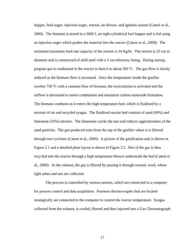
hopper, feed auger, injection auger, reactor, air blower, and ignition system (Cateni et al.,
2000). The biomass is stored in a 5660 L air tight cylindrical fuel hopper and is fed using
an injection auger which pushes the material into the reactor (Cateni et al., 2000). The
estimated maximum feed rate capacity of the reactor is 34 Kg/hr. The reactor is 25 cm in
diameter and is constructed of mild steel with a 5 cm refractory lining. During startup,
propane gas is combusted in the reactor to heat it to about 500 ºC. The gas flow is slowly
reduced as the biomass flow is increased. Once the temperature inside the gasifier
reaches 750 ºC with a constant flow of biomass, the recirculation is activated and the
airflow is decreased to starve combustion and maximize carbon monoxide formation.
The biomass combusts as it enters the high temperature bed, which is fluidized by a
mixture of air and recycled syngas. The fluidized reactor bed consists of sand (90%) and
limestone (10%) mixture. The limestone cracks the tars and reduces agglomeration of the
sand particles. The gas produced exits from the top of the gasifier where it is filtered
through two cyclones (Cateni et al., 2000). A picture of the gasification unit is shown in
Figure 2.1 and a detailed plant layout is shown in Figure 2.1. Part of the gas is then
recycled into the reactor through a high temperature blower underneath the bed (Cateni et
al., 2000). At the exhaust, the gas is filtered by passing it through ceramic wool, where
light ashes and tars are collected.
The process is controlled by various sensors, which are connected to a computer
for process control and data acquisition. Fourteen thermocouples that are located
strategically are connected to the computer to control the reactor temperature. Syngas
collected from the exhaust, is cooled, filtered and then injected into a Gas Chromatograph
17

18
for analysis. The cooled gas is then compressed and filled in storage tanks at 120 psi
(Cateni et al., 2000).
Figure 2.1 Gasifier pilot plant set up

T-1
EQ-1
Air
F
I-1
V--1Air Heater
V--2
T-2
EQ-2 EQ-3
V--3
V--4
V--5
V--6 V--7V--8
V--9
V--10 V--11
T-4T-5
T-3
T-6V--12
V--13 V--14
HX-1
V--15
Water In Water OutT-7 T-8
V--16
V--17 V--18 V--19
V--20
V--21 C1
V--22 V--23
V--24 V--25
T-9
T-10
DV-1
Index
I 1 Mass FlowmeterV1-21 ValvesT 1 Biomass Storage TankEQ 1 Screw FeederT 2 Steam FeederT 3 Gasification UnitEQ 2,3 Cyclone SeparatorsT 4,5 Dust CollectorsT 6 FilterHX 1 Heat ExchangerT 7,8 ScrubbersC 1 CompressorDV 1 Condensate Drain ValveT 9,10 Gas Storage
Figure 2.2 Gasifier pilot plant flowsheet
19

2.2 Syngas Fermentation Synthesis gas is a major building block in the production of fuels and chemicals.
Catalytic processes may be used to convert syngas into a variety of fuels and chemicals
such as methane, methanol, formaldehyde, acetic acid and, ethanol (Klasson et al., 1992).
In 1987, a strict anaerobic mesophilic bacterium was isolated that converted CO, H2, and
CO2 to a mixture of acetate and ethanol. The bacterium was identified and characterized
as a new clostridial species, named Clostridium ljungdahlii (Rajagopalan et al., 2002). In
addition to synthesis gas components, it is also capable of using sugars like xylose,
arabinose, and fructose (Klasson et al., 1990, Klasson et al., 1992). The metabolic
pathway through which CO and CO2 are utilized to produce ethanol is called the acetyl-
CoA pathway or the Wood-Ljungdahl pathway (Wood et al., 1986). The overall
stoichiometry for ethanol formation from CO, CO2 and H2 is (Rajagopalan et al., 2002):
6 CO + 3 H2O C2H5OH + 4 CO2 (2.8)
2 CO2 + 6 H2 C2H5OH + 3 H2O (2.9)
With CO alone as the sole substrate carbon source, one third of the carbon from CO can
be theoretically converted into ethanol (Rajagopalan et al., 2002). A novel clostridial
bacterium, P7 was demonstrated to produce ethanol and acetic acid from CO, CO2 and H2
through an acetogenic pathway (Datar, 2003, Rajagopalan et al., 2002). The optimum
survival growth of P7 is at a pH range of 5-6 (Rajagopalan et al., 2002). The production
of ethanol through the acetyl-CoA pathway using P7 is presently under study at
Oklahoma State University.
20

The choice of a suitable bioreactor for synthesis gas fermentations is a question of
matching reaction kinetics with the capabilities of various reactors. However, for
fermentation processes which involve slightly soluble gases, mass transfer usually
controls the reactor size (Klasson et al., 1992). A good reactor design for a fermentation
process is one, which can achieve high mass transfer rates and high cell growth under
operating conditions in a small reactor volume with minimum operational difficulties and
costs (Datar, 2003). The reactor should then be efficiently scaled up to industrial size for
the integrated gasifier-bioreactor-distillation column plant. Continuous stirred tank
reactors (CSTR) are traditionally used for fermentation processes. A CSTR offers high
rates of mass transfer and agitation leading to a higher conversion of CO into ethanol. A
bubble column reactor offers greater mass transfer than a CSTR for producer gas
fermentations, but initial studies (Rajagopalan, 2001) have indicated that the bioreactor is
limited by the intrinsic kinetics of P7 (nutrient limitation) and not by the mass transfer
rate of CO from the bulk gas to the cells (Datar, 2003). The chemical composition of the
culture medium and nutrient requirements are described elsewhere (Datar et al., 2004).
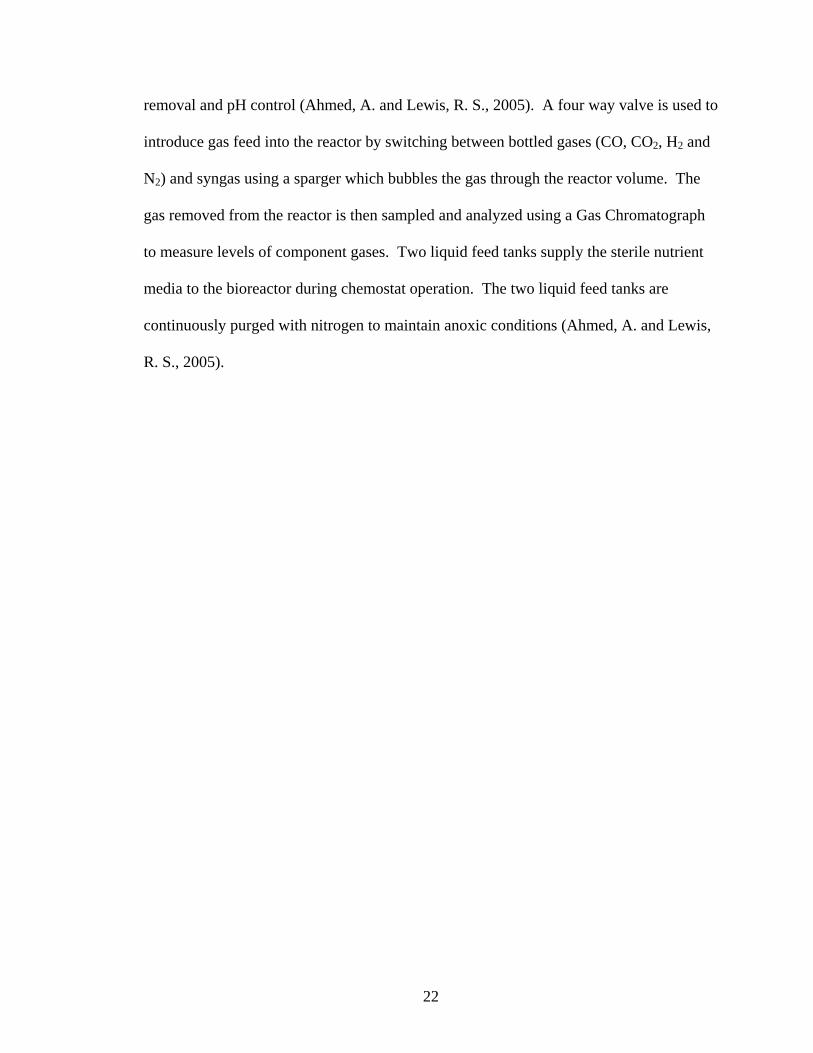
2.2.1 Bioreactor Laboratory Scale Set-up The present bioreactor set up at Oklahoma State University is a BioFlo 110 Bench
top Fermentor (New Brunswick Scientific, Brunswick, NJ) with a 3 liter working
volume, which was used for fermentation studies in a continuous operation mode
(Ahmed, A. and Lewis, R. S., 2005). A detailed schematic diagram is shown in Figure
2.3. The reactor consists of an agitator, sparger, pH probe, dissolved oxygen probe, ports
for liquid inlet and outlet, jacket for temperature control and pumps for feed, product
21
22
removal and pH control (Ahmed, A. and Lewis, R. S., 2005). A four way valve is used to
introduce gas feed into the reactor by switching between bottled gases (CO, CO2, H2 and
N2) and syngas using a sparger which bubbles the gas through the reactor volume. The
gas removed from the reactor is then sampled and analyzed using a Gas Chromatograph
to measure levels of component gases. Two liquid feed tanks supply the sterile nutrient
media to the bioreactor during chemostat operation. The two liquid feed tanks are
continuously purged with nitrogen to maintain anoxic conditions (Ahmed, A. and Lewis,
R. S., 2005).

F
To Distillation Columns
G--1 G--2 G--3 G--4
V--1 V--4V--3V--2
G--5
PV--1
OV--1
BF--1 F--2
HX--1P--1
P--2
M--1 M--2
P--3
F--3
PLC--1
pH--A
BF--2
OV--2
Index
G 1-4 Gas Feed TanksV 1-6 ValvesF Mass Flow ControllerPV 1 Four Way ValveOV 1,2 Open ValvesBF 1,2 Bubble FlowmetersF 2-3 FiltersBR 1 BioreactorP 1-3 Centrifugal PumpsM 1,2 Media TankspH A Acid Storage TankpH A Base Storage TankPLC 1 pH ControllerHX 1 Heat Exchanger
V--5 V--6
pH--B
Figure 2.3 Bioreactor lab scale set up flowsheet
23

2.3 Process Simulation
Simulation can be defined as the use of a mathematical model to generate the
description of the state of a system (Raman, 1985). The biggest advantage of process
simulation is that it provides a good insight into the behavior of an actual process system.
This is particularly true for complex systems with several interacting variables. Since the
computer based mathematical model responds to changes in the same parameters as does
a real process, simulation provides a convenient, inexpensive and safe method of
understanding the process without actually experimenting on an operating process plant
(Raman, 1985). Over the years, computer based process simulation has come a long way
from BASIC and FORTRAN algorithms run on large mainframe computers to modern
and much more complex software packages like Aspen Plus™, ChemShare, ChemCAD,
FLOWTRAN, HYSYS and Pro II that can be run on all types of computers. The
evolution of the personal computer over the past two decades has put the power of
process simulation in the hands of many engineers. A logic flowchart for development
of a process simulation is shown in Figure 2.4.
24

ProcessModel
ThermophysicalProperties
Process DefinitionGlobal Inputs
ComponentSpecification
OperatingConditions
Does it fitexperimental
data ?
Redo Approximations
RobustModel
Predictionsfrom
Model
SensitivityAnalysis
Figure 2.4 Simulation model development algorithm
25

Steady-state simulation is a powerful tool that enables process engineers to study plant
behavior and analyze effects of changes in process parameters by using simulation
software. The Chemical Process Industries have benefited by the use of process
simulation by analyzing new development projects, studying economic feasibility of
upcoming technologies and optimization and de-bottlenecking of existing plants.
Process simulation models are developed using parametric data from existing plants or
the literature. The advantage of modern simulator packages is the built in
thermodynamic models and databanks, which make the task of process calculations on a
computer very simple. A detailed process model fit precisely to plant data allows one to
study the plant and its inefficiencies in depth and helps the engineer to cut costs,
investigate design modifications, optimize the process, increase efficiency, cut down on
cumbersome and expensive experimentation and improve the product quality.
Aspen Plus™ has many advantages as a process simulator. The thermodynamic
models and the unit operation models are already built in, so there is no need to program
them individually. The simulator can easily handle solids, which is a major advantage
over many other software packages. Even with all the built in capabilities, Aspen Plus™
is easily customizable when required (Wooley and Ibsen, 2000). Aspen Plus™ is the
most widely used commercial process simulation software for steady state simulation
(Luyben, 2004). Steady-state simulation in Aspen Plus™ allows the user to predict the
behavior of a system by using basic mass and energy balances, reaction kinetics, phase
and chemical equilibrium. With Aspen Plus™ one can easily manipulate flowsheet
configuration, feed compositions and operating conditions to predict plant behavior and
design better plants.
26

2.3.1 Biomass Gasification Modeling and Simulation
For a clear understanding of the design and operation of a gasifier, complete
knowledge of the effects of operation parameters like fuel, air and operation temperature
is vital. Developing mathematical models for biomass gasification is a complex task due
to the presence of multiple reactions at the high operating temperatures at which
gasification takes place. Although biomass gasification is not a new technology,
pertinent experimental data is incomplete. Consequently, most of the necessary modeling
parameters are usually derived from coal gasification (Bettagli et al., 1995).
Many models for the fluidized bed gasifier are demonstrated in the literature.
These models can chiefly be divided into kinetic models and thermodynamic equilibrium
models. Numerous kinetics based biomass gasification models are illustrated in literature
(Bettagli et al., 1995, Bilodeau et al., 1993, Bingyan et al., 1992, Wang and Kinoshita,
1993). Kinetics based models always contain parameters that make them not universally
applicable to different plants (Schuster et al., 2001). Hence thermodynamic equilibrium
calculations, which are independent of the gasifier design, may be more convenient for
process studies on the influence of important process parameters (Schuster et al., 2001),
although equilibrium models cannot be used to scale up gasifiers. Many equilibrium
based biomass gasifier models are demonstrated in literature (Bridgwater et al., 1989,
Schuster et al., 2001, Wang and Kinoshita, 1992, Watkinson et al., 1991). Schuster et al.
have used a commercial equation-oriented simulation tool IPSEproTM for developing an
equilibrium model for biomass gasification.
27

In this study, biomass gasification using switchgrass as feedstock, was simulated
using a thermodynamic equilibrium model developed in Aspen Plus™. The gasification
model was developed with the following assumptions:
• The gasifier is at steady state operating condition
• The biomass feed is a uniform spherical solids feed
• The biomass undergoes instantaneous devolatilization
• Agglomeration, entrainment and ash formation were neglected
• Ideal mixing of biomass and air inside the reactor
• Ideal gas behavior
• Isothermal behavior of the gasifier
Most of the assumptions are simple and valid, although in practice the ideal mixing is not
observed which gives rise to fluctuations in exit gas composition. Also, the gasifier does
not perform isothermally, the operating temperature is sensitive to variations in moisture
associated with biomass, air feed rate and the biomass feed rate.
2.3.2 Syngas Fermentation Modeling and Simulation
A recent report (Pimentel and Patzek, 2005) vehemently argues that the biomass
generated ethanol manufacturing technology was over hyped and ethanol production
miscalculated, thus rendering the project economically unfeasible. This study aims at
simulation of a syngas fermentation model to study the maximum amount of ethanol
production possible using switchgrass as feedstock. Many kinetics based models were
used earlier to simulate biological reactors (Lee et al., 1983, Mussati et al., 1998, Nihtila
28

et al., 1997), some have also used Finite Element analysis approach for modeling kinetics
based reactors (Kalil et al., 2000, Nihtila et al., 1997).
Simulation of biological processes using commercial simulators is a daunting
task, since most of the commercial simulators are packaged with technology pertaining to
the petroleum industry namely distillation. There are some process simulators like
gPROMS and Berkeley Madonna which are specifically designed for simulation of
biological reactors. These software packages use integrated traditional kinetics models to
simulate the bioreactor. A recent trend in bioreactor simulation is to build a reaction
scheme based on the biological reactions and metabolic pathways and represent them as
parallel or successive elementary reactions. Such an approach is more naturally
integrated into process simulators since they treat reactions in a sequential manner
(Pascal et al., 1995). To be rigorous, a simulation model must use equilibrium conditions
as boundary values. The equilibrium predictions are far from simple because the liquid
phase is a multi component mixture with ionic media (Pascal et al., 1995).
In this study, a fermentation reactor was simulated using two approaches, a
thermodynamic equilibrium approach using Gibbs free energy minimization technique to
calculate the maximum ethanol yield possible and analyze the effect of feed variations in
individual components of syngas and a stoichiometric approach to study the effect of
conversion of CO and H2 on ethanol production. The bioreactor models were developed
using the following assumptions:
• The bioreactor is at steady state operating condition
• Mass transfer limitations do not hinder reactions
• The presence of biological catalyst was neglected
29

• The reactions occurring in the reactor are instantaneous
• The reactor is well mixed and the gas phase is well dispersed in the liquid
phase
• Isothermal behavior of the bioreactor
For the stoichiometry based reactor, a further assumption was the presence of only two
reactions shown by equations 2.8 and 2.9. The assumption of neglecting the biological
catalyst essentially treats the bioreactor as a chemical reactor based on two reactions. For
the equilibrium based model, all possible reactions possible with the present chemical
species at the operating temperature would be taken into account. It was demonstrated
earlier (Rajagopalan, 2001) that the present bioreactor set up is not limited by mass
transfer between the gas phase and the liquid phase, but was limited by intrinsic kinetics
of P7. Thus the assumption of elimination of the microbial catalyst is sound for
evaluating the maximum production of ethanol in a chemical reactor.
The simulation technique for modeling the gasifier and the bioreactor using
Aspen Plus™ is elucidated in the next chapter.
30

CHAPTER 3
DEVELOPMENT OF PROCESS MODELS IN ASPEN PLUS
In this study, a steady state process simulator Aspen Plus™ (Advanced System
for Process ENgineering), which is developed by Aspen Technology was used to develop
process models. Aspen Plus™ is one of the most powerful and widely used process
simulators in the process industry today. It has several features that make it very intuitive
and user friendly. Its Graphic User Interface and Model Manager make an excellent
guide for the user and allow for complete specifications and control at every stage of
model development.
Although Aspen Plus™ is perhaps the most widely used process simulator in the
industry; its usage is not widely reported in literature, since most of the industrial
technical reports are proprietary in nature and not available universally.
3.1 Process Characterization
The fluidized bed gasification process was modeled as a steady state process in
Aspen Plus™. The biomass input stream was assumed to consist of pure elemental solids
and modeled as a combined solids feed stream.
The continuously stirred tank reactor process for anaerobic fermentation was
modeled as a steady state process in Aspen Plus™.
31

3.2 Component Specification Aspen Plus™ has an extensive database for pure component specification and
properties. The built in database contains parameters for almost 8500 components which
include organic, inorganic and salt species (Aspen Tech User Manuals, 2003). The
species present in process feed streams and possible products are defined in the
components specification form. The components specified in the gasifier and the
bioreactor are listed in Table 5.1 and Table 5.3 respectively.
3.3 Physical Property Estimation
Estimation of accurate thermodynamic properties of pure components and
mixtures in a process is vital for any process (Carlson, 1996). Property estimation in
Aspen Plus™ can be performed using more than 80 EOS based thermodynamic models
built in the simulator. Binary interaction parameters are determined data from
DECHEMA (Aspen Tech User Manuals, 2003).
Properties for the components in the gasifier model were calculated from the
SOLIDS Equation Of State (EOS) based property estimator since it is the recommended
property estimator for solids. One reason for choosing Aspen Plus™ as a simulator over
other simulation softwares was because it allows the user to include solids in the
simulated process models. Properties for the components in the bioreactor simulation
model were evaluated using the Non-Random Two Liquid (NRTL) model based
estimator since the system is a Vapor-Liquid System (VLE) system operating at a
pressure of less than 10 atmospheres with an assumption of the media as a non-electrolyte
and the NRTL method is recommended for such conditions (Carlson, 1996).
32

33
3.4 Built-In Reactor Models in Aspen Plus
Aspen Plus™ has a Model Library which is equipped with reactor models chiefly
categorized as: (a) Balance or stoichiometry based reactors (b) Equilibrium based
reactors (c) Kinetics based reactors. Since reaction kinetics for both the gasifier and
bioreactor are not well documented for the experimental studies at Oklahoma State
University, kinetics based models were not used. The Gibbs reactor model in Aspen
Plus™ is the only reactor model which calculates solid-liquid-vapor equilibrium,
considers simultaneous phase and chemical equilibria and has a temperature based
approach to equilibrium (Aspen Tech User Manuals, 2003). Hence it makes the most
suitable reactor model for simulating the gasifier. For modeling the bioreactor, a balance
based stoichiometric reactor model and an equilibrium based Gibbs reactor model were
used.
3.5 Process Flowsheet Development
The Process Flowsheet Window and the Model Library in Aspen Plus™ allow the
user to construct the flowsheet graphically (Aspen Tech User Manuals, 2003). The
model library is equipped with an array of process equipments, modifiers and connectors
from which a process plant and its sections can be designed. The flowsheet developed
for the bioreactor based on the stoichiometric reactor model is shown in Figure 3.1.

298
121590
GASES
298
121590
MEDIA
310
101325
PRODUCT
310
101325
PRODGAS
310
101325
PRODMED
RSTOIC SEP2Temperature (K)
Pressure (N/sqm)
Figure 3.1 Flowsheet of the bioreactor simulation using a stoichiometric reactor model in Aspen PlusTM
34

3.6 Process Variables Specification
The state variables for the system like temperature, pressure and flowrate are
designated in the specifications input form. Molar compositions of the input gas streams
for the gasifier and the bioreactor are defined in this section. A snapshot of a
Specification Form is shown in Figure 3.2.
3.7 Sensitivity Analysis Tools
Aspen Plus™ equips the user with an array of model analysis tools like
Sensitivity Analysis, Data Fit, Optimization and Constraint Analysis (Aspen Tech User
Manuals, 2003). The sensitivity analysis tool was used in this study to analyze and
predict the behavior of the model to changes in key operating and design variables.
Process variables like temperature and Air Fuel ratio were varied to study the
effect on the exhaust gas composition of the gasifier. Feed composition of input gases to
the bioreactor was varied to study the effect on ethanol production. These studies are
helpful in predicting scenarios over a range of operating variables and provide solutions
in a “What-If” analysis.
3.8 Simulation Output Data
Simulation results in Aspen Plus™ are reported on the Results Data Form and are
segregated as a global output and a streams summary. The global output reports the
overall mass balance, overall heat balance, heat duty and, reaction enthalpies. The stream
results summarize the stream flowrates, stream compositions, individual stream fractions,
35

stream flowrates, stream entropies, stream enthalpies, average densities and, molecular
weights.
Figure 3.2 Snapshot of a typical specifications input form in Aspen PlusTM
36

CHAPTER 4
MODELING OF A GASIFIER AND A BIOREACTOR 4.1 Modeling a Gasifier as a Gibbs Reactor Model The gasification process at Oklahoma State University is carried out in a pilot
plant scale fluidized bed gasifier. A gasifier model in Aspen Plus™ was used for
simulation with the assumption that the gasifier reaches physical and chemical
equilibrium at the operating conditions and hence a Gibbs free energy minimization
model denoted by RGibbs, can be used to simulate it. The built-in RGibbs reactor model
of Aspen Plus™ is the only unit operations model that can compute a solid-liquid-vapor
phase equilibrium. The model uses Gibbs free energy minimization with phase splitting
to calculate equilibrium without the need to specify stoichiometry or reaction kinetics
(Aspen Tech User Manuals, 2003).
RGibbs considers each solid stream component as a pure solid phase unless
specified otherwise. The biomass input stream was specified with C, H, N and O as
individual components. Reported experimental data shows an absence of sulfur in the
standard run, in some other runs of the gasifier a trace amount of less than 0.01 % by
weight has been reported. For this study, the presence of sulfur in biomass was assumed
to be zero. Possible products of gasification that were identified in the reactor model are
C, H2, N2, O2, H2O, CO, CO2, CH4, C2H2, C2H4, NO, NO2, N2O, NH3 and HNO3. Oxides
37

of sulfur are ruled out since sulfur was not identified as a component in the reactor. A
complete list of input components is shown in Table 5.1.
4.1.1 Base Case Simulation
A model was developed on the basis of input data from a standard experimental
run of the gasifier. The composition of input biomass stream in the simulation was
duplicated from the experimental run and is listed in Table 5.1. The biomass input
stream is fed to the reactor at 25 ºC and 1.2 atm pressure. The air input stream was also
fed to the reactor at 25 ºC and 1.2 atm pressure. Biomass was fed at a rate of 17.64 Kg/hr
and air was fed at a rate of 30.13 Kg/hr. The reactor operating conditions were specified
at 815 ºC and 1.0 atm, with a temperature approach to equilibrium for the reactor.
Thermodynamic properties of the components were calculated for the model using the
SOLIDS EOS based property estimator in Aspen Plus™.
4.1.2 Fuel Sensitivity Analysis
This analysis was conducted to study the effect of a change in the biomass feed
rate on the exhaust gas composition, while maintaining the biomass elemental
composition the same as the base case. A sensitivity analysis tool was implemented as a
nested loop in the model developed for the base case scenario. Biomass feed in 34 runs
reported by the gasifier research group varied from 12.01 to 23.15 Kg/hr (including
moisture). The fuel or biomass input in the sensitivity model was varied from12.0 Kg/hr
to 24.0 Kg/hr (including moisture). Operating conditions for all other streams and the
reactor remained the same as the base case.
38

4.1.3 Moisture Sensitivity Analysis The biomass is generally associated with some moisture when fed to the reactor.
This analysis was conducted to study the effect of variation in the moisture content of the
biomass on the composition of exhaust gases from the gasifier. The experimental range
of moisture associated with biomass was 1.13 Kg/hr to 5.99 Kg/hr. The H2O content in
the biomass input stream to the reactor was varied from 0.5 Kg/hr to 8.0 Kg/hr.
Operating conditions for the air feed stream and the reactor remained same as the base
case.
4.1.4 Temperature Sensitivity Analysis
In a gasification process, reactor temperature is a key variable since it affects
equilibrium thermodynamics. In this analysis, the reactor temperature was varied to
study the effects on the output gas composition and individual gas flowrates in the
exhaust stream. The range of temperatures over which the pilot plant was tested is 635
ºC to 850 ºC. In the simulated model the temperature was varied from 600 ºC to 900 ºC.
All other operating conditions remained the same as the base case model.
4.1.5 Air Fuel Ratio Sensitivity Analysis
A term widely used in gasification technology is Air Fuel Ratio since it has a
strong effect on the process. The Air Fuel (AF) ratio is defined as:
BiomassDryofWeightAirofWeightAF = (4.1)
The AF ratio is a key variable because an increase in it causes an increase in the amount
of oxidant and hence a shift in the gasifier operation from pyrolysis to gasification and
39

further on towards total combustion. A comparative study of the producer gas quality
and energy conversion efficiency of various gasifiers shows that these parameters are
predicated by the AF ratio (Esplin et al., 1986). In this analysis the AF ratio was varied
from a value of 1.1 to 3.31 and the effect on product gas flow rates and mole fractions of
individual gas components charted. Other operating parameters for the model remained
same as the base case model.
4.1.6 Equivalence Ratio Sensitivity Analysis
A concept frequently used in gasification technology is the Equivalence Ratio
(ER), which is defined as the oxidant to fuel ratio divided by the stoichiometric ratio.
RatioBiomasstoAirtricStoichiomeBiomassDryofWeightAirofWeightER = (4.2)
The ER should be greater or equal to 1.0 for complete combustion of fuel to carbon
dioxide and water (Reed, 1981). Complete combustion of wood biomass requires 6.364 g
air/g wood (Reed, 1981). For this analysis, switchgrass composition is assumed to be
same as the elemental composition of wood as CH1.4O0.59N0.1 (Reed, 1981). The ER is
frequently manipulated in gasification technological models to study its effect on gasifier
performance. The ER determines the fraction of fuel that is gasified in the reactor as well
as affects the fluidization quality and the reactor temperature (Natarajan et al., 1998). In
this analysis, the ER was manipulated over a range of 0.17 to 0.53 to study its effect on
the exhaust gas composition. Other process parameters for reactor operation remained
same as the base case model.
40

4.2 Bioreactor Modeling in a Gibbs Reactor Model Syngas fermentation to produce ethanol is performed in a laboratory scale
biofermentor at Oklahoma State University. Kinetics of the fermentation reactions to
produce ethanol is not well quantified. A bioreactor model developed in Aspen Plus™
was designed with the assumption that the CSTR attains chemical and phase equilibrium
at the operating temperature and pressure and hence it can be simulated using a Gibbs
reactor model. The Gibbs reactor model does not take microbial growth into account as a
catalyst for the conversion of syngas to ethanol. Although treatment of the bioreactor as
a chemical reactor without microbial catalyst is not accurate, this analysis was conducted
to study the maximum amount of ethanol that can be produced in a Gibbs free energy
model. Sensitivity analyses based on this model were conducted to study the effects of
variation in individual feed gas compositions on bioreactor performance.
Thermodynamic properties for the components were calculated using an NRTL based
property estimator in Aspen Plus™, since the bioreactor is a liquid-liquid equilibrium
model, properties for which are best predicted using the NRTL based model (Carlson,
1996).
The syngas stream to the bioreactor model was assumed to be composed only of
CO, CO2, H2 and N2. Presence of trace gases and hydrocarbons were neglected since
their combined mole fraction contribution to the stream is about 1%. Presence of
methane in the exhaust stream of the gasifier has not been taken into account since it
causes a drastic reduction in the ethanol produced in the model; this is discussed in a later
section.
41

The media fed to the bioreactor contains a solution of nutrients in water, which
are necessary for microbial growth. In the simulated model, the media feed stream is
assumed to be pure water. Possible products from the model were identified as C2H5OH,
H2O, CO, CO2, H2 and N2. Butanol and Acetic Acid, which are usually associated as by
products in syngas fermentation have not been taken into consideration as possible
products, since the focus of this work was on ethanol production. A complete list of
input components and specification data is shown in Table 5.3. The product stream from
the model was split using a phase separator, into a gas phase output stream containing the
gases CO, CO2, H2 and N2 and a liquid phase output stream containing C2H5OH and H2O.
4.2.1 Base Case Simulation
The model was developed on the basis of data from an experimental run of the
bioreactor. Input gas and media streams were fed at 25 ºC and 1.2 atm pressure each.
The gas composition and flowrates are tabulated in Table 5.3. The reactor operating
conditions were specified at 37 ºC and 1.0 atm pressure, with a temperature approach to
equilibrium.
4.2.2 Carbon Monoxide Sensitivity Analysis
This analysis was conducted to study the effect of variation in the CO molar
composition in the feed gas stream on the ethanol produced in the bioreactor. The
analysis was performed using output data from a set of 17 simulation runs of the model
developed for the base case scenario. The exhaust gas composition data from the gasifier
experimental runs was used for this analysis, due to the lack of a range of data from the
42

laboratory bioreactor runs. Trace gases and hydrocarbons present in the exhaust gas
stream of the gasifier were not considered and were compensated by difference in the
percentage composition value of N2. In the feed gas stream the mole fraction of CO was
varied while keeping the mole fractions of CO2 and H2 constant. A change in the mole
fraction of CO was compensated by difference with a change in the mole fraction of N2,
since variation of N2 does not affect bioreactor performance as it is an inert component.
The mole fraction of CO was varied from 0.1 to 0.2 in the simulation runs while keeping
the mole fraction of CO2 at a constant of 0.1871 and the mole fraction of H2 at 0.0525.
The mole fraction of N2 was varied to adjust variations in the mole fraction of CO. Other
operating conditions in the model remained the same as the base case model.
4.2.3 Carbon Dioxide Sensitivity Analysis
This analysis studied the effect of variation in the mole fraction of CO2 in the feed
gas on the ethanol produced. The analysis is based on output data from a set of 18
simulation runs of the model developed using the base case. The mole fraction of CO2
was varied in the feed stream while keeping the mole fractions of CO and H2 constant at
the average gasifier output level. Presence of trace gases and hydrocarbons in the gasifier
exhaust was neglected in the input gas feed stream to the bioreactor as discussed earlier.
The mole fraction of CO2 varied in the experimental runs from 0.1774 to 0.2055. In the
simulation analysis model, the mole fraction of CO2 was varied from 0.11 to 0.25. The
mole fraction of N2 was varied in the feed by a difference to compensate for variation in
the mole fraction of CO2. Mole fraction of CO was held at a constant of 0.1407 and mole
43

fraction of H2 was kept constant at 0.0525. All other operating conditions for the streams
and reactor remained same as the base case model.
4.2.4 Hydrogen Sensitivity Analysis
This study delineated the effect of variation in the mole fraction of H2 in feed gas
to the bioreactor on the ethanol produced in the model. The analysis is based on output
data from a set of 16 simulation runs of the model developed using the base case. The
mole fraction of H2 was varied in the gas feed, while keeping the mole fractions of CO
and CO2 constant at 0.1407 and 0.1871 respectively. Presence of trace gases and
hydrocarbons in the gasifier exhaust gas was neglected as discussed earlier. In the
experimental runs of the gasifier, the composition of H2 varied from a mole fraction of
0.0379 to 0.0627. Mole fraction of H2 in the simulated runs was varied from 0.03 to 0.09
while maintaining CO and CO2 at constant mole fractions of 0.1407 and 0.1871
respectively. All other operating conditions for the streams and the reactor remained
same as the base case model.
4.2.5 Media Sensitivity Analysis
The media feed to the bioreactor was assumed as a pure water feed stream to the
Gibbs reactor model. This analysis presents the effect of variation of water input to the
reactor on the liquid phase output composition from the reactor model. The water input
to the reactor was varied using a sensitivity analysis tool built as a nested loop in the
process model and the exit mole fractions of water and ethanol were charted. In the
laboratory experiments on the bioreactor, media feed is usually varied from a flowrate of
44

0.2 to 2.5 ml/min or 3.3 E-6 Kg/sec to 4.1 E-6 Kg/sec. In this analysis the water input
flowrate was varied from 1.0 E-6 Kg/sec to 5.0 E-5 Kg/sec. The gas composition was
kept at constant mole fractions of CO: 0.1407, CO2: 0.1871, H2: 0.0525 and N2: 0.6197.
All other process parameters remained same as the base case model.
4.3 Bioreactor Modeling in a Stoichiometric Reactor Model
Ethanol production from syngas can be stoichiometrically represented by the
reactions shown by equations 2.8 and 2.9. The syngas is composed mainly of CO, CO2,
H2 and N2 gases. The exhaust gas from the gasifier contains a small fraction of methane
but its presence was shown to reduce the production of ethanol in the simulated model,
which is discussed in a later section. Other trace hydrocarbons emanating from the
gasifier were assumed to be negligible for reactor modeling in Aspen Plus™. Since
reaction kinetics for the bioreactor is not well quantified and a kinetic model for the
bioreactor not yet developed, a kinetics approach for the reactor cannot be accurately
modeled. The stoichiometric reactor model developed in Aspen Plus™ performs mass
and energy balances based on the reaction stoichiometry and extent of conversions of the
reactants.
For the bioreactor modeling in a stoichiometric reactor model, it was assumed that
only the above mentioned reactions are occurring in the bioreactor. The individual
effects of the two reactions on ethanol production and reactant consumption were studied
in this analysis. The effect of microbial growth and catalytic behavior of the organism on
reactant consumption was not taken into consideration. The syngas feed to the bioreactor
was assumed to be comprised of pure CO, CO2, H2 and N2 gases. Presence of methane
45
and other hydrocarbons in the gasifier exhaust gas were neglected in the gas feed stream
to the model. The media fed to the bioreactor contains nutrients necessary for microbial
growth. The media feed stream in the model was defined as a pure water stream.
CO, CO2, H2, N2, H2O and C2H5OH were defined as possible products from the
bioreactor. Experimental runs of the bioreactor show a production of butanol and acetic
acid as well; these have not been taken into consideration in the simulated model since
only the production of ethanol was under study. A complete list of input components is
specified in Table 5.3. The product stream from the reactor was split into a gas phase
containing CO, CO2, H2 and N2 and a liquid phase containing H2O and C2H5OH using a
phase separator.
4.3.1 Base Case Simulation
A base case simulation was developed on the basis of experimental data from a
laboratory run of the bioreactor. The gas and media streams were fed to the reactor at 25
ºC and 1.2 atm pressure each. Stream composition and flowrate specifics are listed in
Table 5.3. Reactions 2.8 and 2.9 were specified occurring in the reactor at 37 ºC and 1.0
atm pressure. For reaction 2.8 the limiting reactant is CO and for reaction 2.9 the
limiting reactant is H2. The extents of both the reactions were individually varied by trial
and error until the composition of exit gases closely matched composition of exit gas in
the experimental run. The product stream from the reactor was split into a gas phase
containing CO, CO2, H2 and N2 and a liquid phase containing H2O and C2H5OH using a
phase separator.
46

4.3.2 Sensitivity of the Model to Stoichiometric Conversions
Extents of reactions 2.8 and 2.9, defined as variables E1 and E2, were manipulated
for the base case analysis and output of the experimental results closely matched at E1 =
0.1 and E2 = 0.1. For this analysis, E1 and E2 were varied individually and
simultaneously to study the effects on exit gas compositions and ethanol production from
the simulated model. Individual extents of reaction can be defined in Aspen Plus™ using
the reaction stoichiometry form, shown in Figure 4.1. The extents of reactions were also
varied using a sensitivity model built as a nested loop in the simulation.
47

Figure 4.1 A snapshot of a typical reaction stoichiometry input form in a stoichiometric
reactor model developed in Aspen PlusTM
48
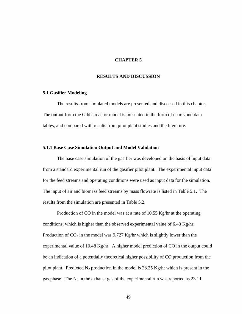
CHAPTER 5
RESULTS AND DISCUSSION
5.1 Gasifier Modeling The results from simulated models are presented and discussed in this chapter.
The output from the Gibbs reactor model is presented in the form of charts and data
tables, and compared with results from pilot plant studies and the literature.
5.1.1 Base Case Simulation Output and Model Validation
The base case simulation of the gasifier was developed on the basis of input data
from a standard experimental run of the gasifier pilot plant. The experimental input data
for the feed streams and operating conditions were used as input data for the simulation.
The input of air and biomass feed streams by mass flowrate is listed in Table 5.1. The
results from the simulation are presented in Table 5.2.
Production of CO in the model was at a rate of 10.55 Kg/hr at the operating
conditions, which is higher than the observed experimental value of 6.43 Kg/hr.
Production of CO2 in the model was 9.727 Kg/hr which is slightly lower than the
experimental value of 10.48 Kg/hr. A higher model prediction of CO in the output could
be an indication of a potentially theoretical higher possibility of CO production from the
pilot plant. Predicted N2 production in the model is 23.25 Kg/hr which is present in the
gas phase. The N2 in the exhaust gas of the experimental run was reported as 23.11
49

Kg/hr. N2 input to the model in the input air stream was 23.11 Kg/hr and in the biomass
stream was 0.14 Kg/hr. Hence the theoretical prediction from the model indicates
complete conversion of N2 into gas phase and emission as exhaust gas. This indicates that
the behavior of N2 is completely inert in the gasification unit. In the experimental run,
some amount of N2 might have been lost as solids in ash and tar, which is not present in
theoretical calculations of the simulated model. The other possibility is experimental
error since N2 is calculated experimentally by difference.
Table 5.1 Experimental input composition of feed streams to gasifier Element/ Gas Kg/hr
N2 23.11
Air O2 7.02 Total 30.13 C 7.18 H 0.91 N 0.14
Switchgrass O 7.77 S 0.00 Ash 0.55 H2O 1.64 Total 18.19
50
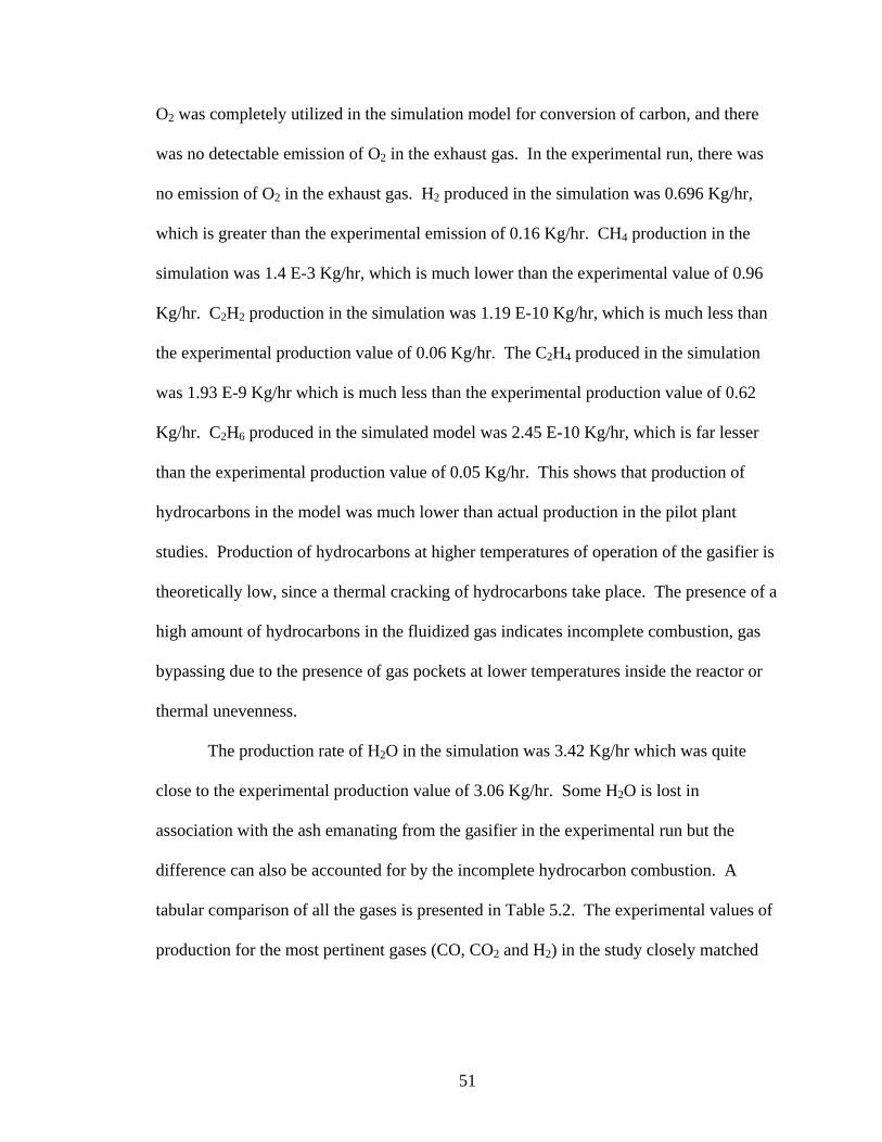
O2 was completely utilized in the simulation model for conversion of carbon, and there
was no detectable emission of O2 in the exhaust gas. In the experimental run, there was
no emission of O2 in the exhaust gas. H2 produced in the simulation was 0.696 Kg/hr,
which is greater than the experimental emission of 0.16 Kg/hr. CH4 production in the
simulation was 1.4 E-3 Kg/hr, which is much lower than the experimental value of 0.96
Kg/hr. C2H2 production in the simulation was 1.19 E-10 Kg/hr, which is much less than
the experimental production value of 0.06 Kg/hr. The C2H4 produced in the simulation
was 1.93 E-9 Kg/hr which is much less than the experimental production value of 0.62
Kg/hr. C2H6 produced in the simulated model was 2.45 E-10 Kg/hr, which is far lesser
than the experimental production value of 0.05 Kg/hr. This shows that production of
hydrocarbons in the model was much lower than actual production in the pilot plant
studies. Production of hydrocarbons at higher temperatures of operation of the gasifier is
theoretically low, since a thermal cracking of hydrocarbons take place. The presence of a
high amount of hydrocarbons in the fluidized gas indicates incomplete combustion, gas
bypassing due to the presence of gas pockets at lower temperatures inside the reactor or
thermal unevenness.
The production rate of H2O in the simulation was 3.42 Kg/hr which was quite
close to the experimental production value of 3.06 Kg/hr. Some H2O is lost in
association with the ash emanating from the gasifier in the experimental run but the
difference can also be accounted for by the incomplete hydrocarbon combustion. A
tabular comparison of all the gases is presented in Table 5.2. The experimental values of
production for the most pertinent gases (CO, CO2 and H2) in the study closely matched
51

the simulation and can be assumed to be generally predictive. A complete list of
components in the product gas is shown in Appendix A.1.
Table 5.2 Comparison of simulation and experimental data
Gas Experimental Output Simulation Output Kg/hr Kg/hr
H2 0.16 0.696 N2 23.11 23.250 O2 0.00 0.000 CO 6.43 10.550
Exhaust Gases CH4 0.96 1.40 E-3 CO2 10.48 9.727 C2H2 0.06 1.19 E-10 C2H4 0.62 1.93 E-9 C2H6 0.05 2.45 E-10 H2O 3.06 3.543
52
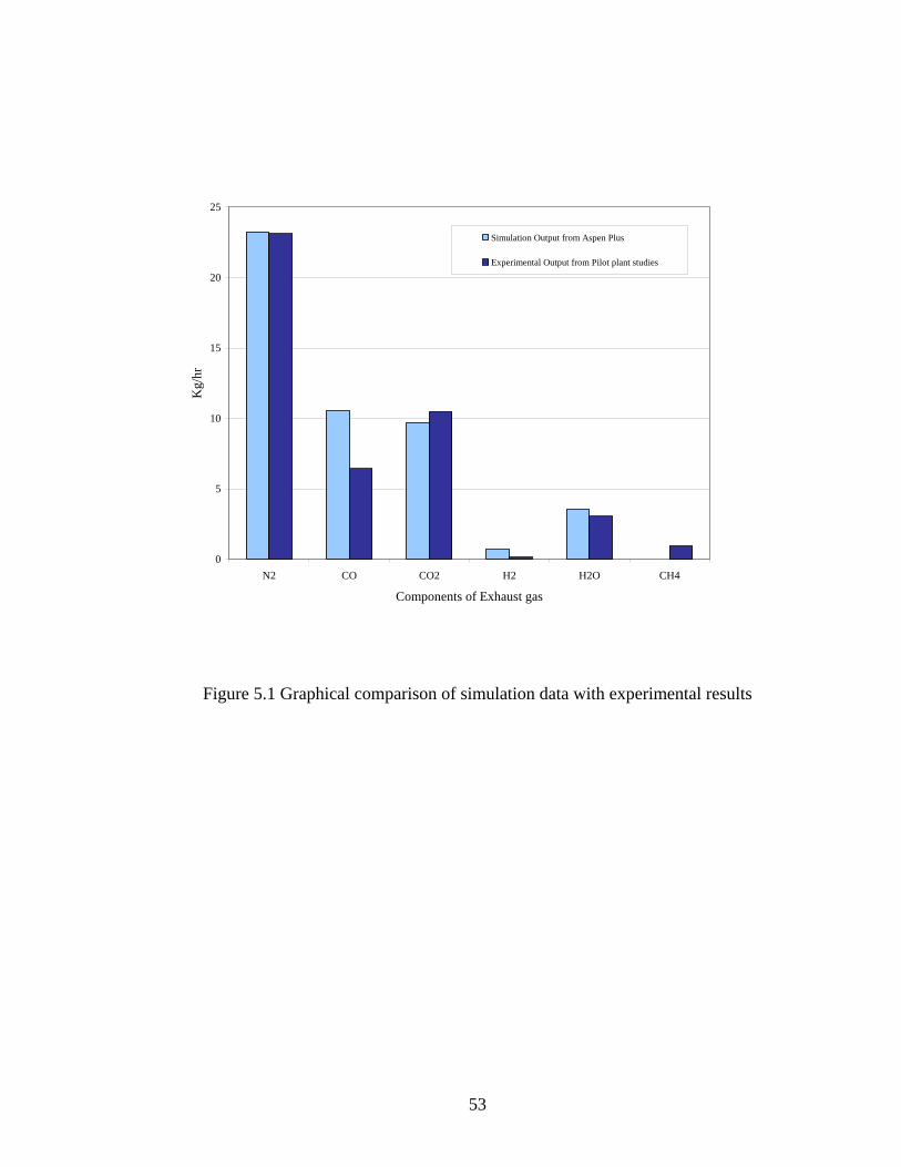
0
5
10
15
20
25
N2 CO CO2 H2 H2O CH4
Components of Exhaust gas
Kg/
hr
Simulation Output from Aspen Plus
Experimental Output from Pilot plant studies
Figure 5.1 Graphical comparison of simulation data with experimental results
53

5.1.2 Effect of Fuel Variation on Production of Syngas
The input biomass feed to the simulation was varied from 12.0 Kg/hr to 24.0
Kg/hr and individual gas production rates in the exhaust gas stream compared with the
variation in biomass feed. The results from this sensitivity analysis are charted in Figure
5.2. There was a linear increase in production of CO with an increase in biomass feed.
This indicates that the majority of conversion of biomass is predicted to go to CO in a
Gibbs reactor model. There was also an increase in the production of H2 with an increase
in the biomass feed. There is a slight reduction in H2O levels produced in the reactor
with an increase in the biomass feed. This indicates a prediction of almost complete
conversion of elemental H in the biomass feed to gaseous H2; only a small fraction of
elemental H gets converted into hydrocarbons. A decrease in the production of CO2 was
also shown in the simulation output. This could be partially the result of a decrease in the
Air Fuel ratio and hence lesser conversion of the fuel to CO2 by combustion. However a
more likely possibility, since there is a simultaneous decrease of H2O and increase of H2
in the model, is that the changes observed are a result of the effect of the water-gas shift
reaction occurring in the reactor at the operating temperature. Production of CH4 in the
model increased with an increase in biomass feed. The production figures were extremely
small to be compared on the same scale as the other gases and were omitted in the chart.
The increase in hydrocarbons with an increase in biomass feed is a result of the change in
the Air to Fuel ratio. Production of N2 increased linearly with biomass feed which shows
conversion of organic N present in biomass into N2 gas.
54

0.0
5.0
10.0
15.0
20.0
25.0
11.0 13.0 15.0 17.0 19.0 21.0 23.0 25.0 27.0
Biomass Flowrate (Kg/hr)
Exha
ust G
ases
Flo
wra
te (K
g/hr
)H2
N2
CO
CO2
H2O
Operatingpoint
Operating Range
Operating Point
Figure 5.2 Effect of variation in the biomass feed rate on the exhaust gas composition
5.1.3 Effect of Moisture Variation on Production of Syngas The moisture associated with biomass in the feed stream was varied from 0.5
Kg/hr to 8.0 Kg/hr while keeping the biomass (dry basis) at a constant feed of 16.0 Kg/hr
and its composition the same as the base case model to model natural moisture content
variability and effect on syngas composition. The results from this analysis are charted in
Figure 5.3. An increase of H2O in the exhaust gas was noted, although the increase was
not linearly proportional with the input of H2O to the model. An increase in CO2 shows
strong indication of the action of the water-gas shift reaction in the model since it is
accompanied by a decrease in CO output. There is also an increase in production of H2
55

which further supports the action of the water-gas shift reaction. An increase of CO2
could also mean an increase in combustion due to increased amount of oxidant in the
reactor. A part of the decrease in CO production could be attributed to the conversion of
CO to CO2 due to higher oxidation in the model. This is also shown by a decrease in the
production of CH4 with an increase in the moisture associated with the biomass feed.
The curve trends for all the gases in this analysis completely match with results from a
computer generated equilibrium model for a fluidized bed gasifier found in literature
(Bridgewater et al., 1989).
0.0
2.0
4.0
6.0
8.0
10.0
12.0
14.0
16.0
0.0 1.0 2.0 3.0 4.0 5.0 6.0 7.0 8.0 9.0
Moisture in Biomass (Kg/hr)
Prod
uct G
ases
(Kg/
hr)
H2O
CO
CO2
H2
CH4
Operating Range
Operating Point
Figure 5.3 Effect of variation in the moisture associated with biomass feed rate on the
exhaust gas composition
56

5.1.4 Effect of Temperature Variation on Syngas Production Temperature is a key variable in a gasification process since most of the reactions
occurring in the reactor are sensitive to temperature and the gasifier operates over a broad
range of temperatures. In this analysis, the temperature was varied from 873 K to 1123
K while keeping the biomass and air feed rates at the base case values. Operational
variables of the reactor remained same as the base case simulation. Production of CO
increased from 7.219 Kg/hr to 11.05 Kg/hr over the range of 300 K with the same
biomass input. This indicates the sensitivity of CO production to temperature and
suggests the possibility to control CO production by manipulating temperature. The
production of CO2 dropped from 13.469 Kg/hr to 8.946 Kg/hr in the temperature interval.
Production of N2 remained constant at a value of 23.250 Kg/hr. Since this is a very high
value as compared to the production values of other gases, it was not included in the
following production profile charts. A production chart on mass basis of gases is
compared with the increase in operation temperature and shown in Figure 5.4.
To better understand the relative behavior of the individual gases, a mole fraction
basis chart is shown in Figure 5.5. An increase in the mole fraction of CO is observed
with an increase in the operating temperature which is similar to the trends found in the
literature (Wang and Kinoshita, 1992, Wang and Kinoshita, 1993). A decrease in the
mole fraction of CO2 in the output correlated with an increase in the operating
temperature, a trend that is also found in the literature (Wang and Kinoshita, 1992,
Bingyan et al., 1992, Wang and Kinoshita, 1993). The mole fraction of H2 reaches a
maximum value a temperature of 948 K but then decreases on a further increase in
temperature.
57

0.0
3.0
6.0
9.0
12.0
15.0
18.0
21.0
24.0
27.0
850 875 900 925 950 975 1000 1025 1050 1075 1100 1125 1150 1175 1200
Temperature (K)
Exha
ust G
ases
Flo
wra
te (K
g/hr
)
H2
N2
CO
CO2
CH4
Operating Range
Operating Point
Figure 5.4 Effect of variation in the operation temperature on the exhaust gas
composition: mass basis
Since the temperature range is above our experimental pyrolysis temperature (<
873 K) and lower than the total combustion temperature (>1200 K), the effect of water-
gas shift reaction is most visible. The curve characteristics of gas mole fractions closely
match those found in literature for biomass gasification in air (Reed, 1981, Wang and
Kinoshita, 1992, Watkinson et al., 1991), and are in complete agreement with a modeling
study using IPSEproTM simulator (Schuster et al., 2001) and a computer program
developed for simulation of biomass gasification under equilibrium conditions (Kinoshita
et al., 1991). The variation in the mole fractions of CO, H2 and CH4 is closely matched
with previous studies using a mathematical model for biomass gasification (Bilodeau et
58

al., 1993, Watkinson et al., 1991) and experimental studies on biomass gasification
(Wang and Kinoshita, 1992). The mole fraction of CH4 decreases with an increase in
temperature, which is also seen in experimental studies in the literature (Wang and
Kinoshita, 1992, Watkinson et al., 1991). This could be attributed to a reverse
methanation reaction occurring in the gasifier at the operation temperature.
0.00
0.05
0.10
0.15
0.20
0.25
850 875 900 925 950 975 1000 1025 1050 1075 1100 1125 1150 1175 1200
Temperature (K)
Exha
ust G
ases
(mol
frac
tion)
H2
CO
CO2
CH4
Operatingpoint
Operating Range
Operating Point
Figure 5.5 Effect of variation in the operation temperature on the exhaust gas
composition: mole basis
Although in this analysis a simple change in temperature has been used to study a
variation in output gas composition, such a change is not possible in actual operation. To
vary the temperature, a change in the Air Fuel ratio is required which changes the amount
of combustion and hence the thermal output in the reactor which in turn affects the
59

operation temperature. However there are thermal losses from the gasifier, either due to
operational heat losses or due to calorific loss to the moisture present (Bridgewater et al.,
1989). Results from this analysis can be used to study other biomass feeds which may
have a different moisture content and hence a different operational temperature for the
same Air Fuel ratio. The hydrocarbons C2H2, C2H4 and C2H6 were produced in trace
quantities in the simulation and decreased with an increase in the operation temperature.
The variation in the mole fraction of these three hydrocarbons on a logarithmic scale is
charted against the variation in temperature and is shown in Figure 5.6.
1.00E-13
1.00E-12
1.00E-11
1.00E-10
1.00E-09
1.00E-08
1.00E-07
1.00E-06
1.00E-05
873 898 923 948 973 998 1023 1048 1073 1088 1098 1123 1148 1173
Temperature (K)
Mol
Fra
ctio
n
C2H2 Mol Fraction in Exhaust GasC2H4 Mol Fraction in Exhaust GasC2H6 Mol Fraction in Exhaust Gas
Figure 5.6 Effect of variation in the operation temperature on the hydrocarbons in the
exhaust gas
60

5.1.5 Effect of Air Fuel Ratio on Syngas Production Air Fuel (AF) ratio is an important variable in gasifier operation. In this analysis,
the air feed rate was varied from 20.0 Kg/hr to 61.0 Kg/hr while keeping the biomass
feed rate constant at the base case value; thus varying the AF ratio from 1.10 to 3.36.
The reactor temperature and all other operating conditions were kept constant at the base
case values. Production of CO decreased from 12.715 Kg/hr to 3.965 Kg/hr over the
manipulated range of AF ratios. Production of CO2 increased from 6.314 Kg/hr to
20.079 Kg/hr. The O2 output remained zero at all times. The variation of individual
gases on a mass flow basis is charted against the AF ratio in Figure 5.7.
0.0
5.0
10.0
15.0
20.0
25.0
30.0
35.0
40.0
45.0
50.0
0.8 1.0 1.2 1.4 1.6 1.8 2.0 2.2 2.4 2.6 2.8 3.0 3.2 3.4 3.6
Air Fuel Ratio
Prod
uct g
ases
(Kg/
hr)
H2
H2O
CO
CO2
N2
Operating Point
Figure 5.7 Effect of variation in the Air – Fuel Ratio on the exhaust gas composition:
mass basis
61

To better understand the relative changes of the individual gases a mole fraction
basis chart for the major product gases is shown in Figure 5.8. The mole fraction of N2
increases with an increase in the AF ratio; this indicates the increase in N2 production
which is associated with an increase in the air feed to the reactor. An increase in the AF
ratio suggests an increase in oxidation of the fuel, hence a higher production of CO2 from
elemental C and more conversion of CO into CO2. This is also indicated by the decrease
in the mole fraction curve of CO with a simultaneous increase in the mole fraction of
CO2. A high amount of CO2 present in the reactor tends to shift the equilibrium of the
water gas shift reaction towards greater production of H2O at higher temperatures.
This is seen in the increasing trend of the H2O mole fraction curve with an increase in
AF. The amount of CH4 produced decreased from 0.006 Kg/hr to 0.0 Kg/hr with an
increase in the AF ratio. This could be either the effect of increased combustion or an
effect of thermal cracking due to a higher internal energy of the reacting species, since
the reactor temperature is kept at the base case constant of 815 °C. Similar trend of CH4
variation were seen for coal gasification at 800-900 °C and 1 bar (Richard et al., 1989).
62
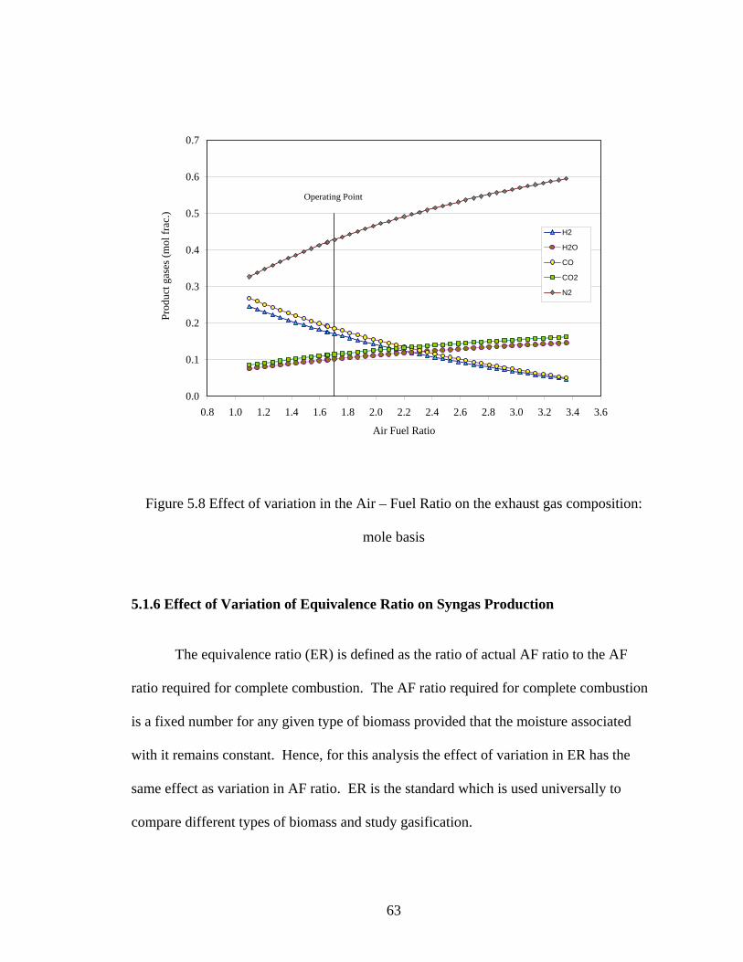
0.0
0.1
0.2
0.3
0.4
0.5
0.6
0.7
0.8 1.0 1.2 1.4 1.6 1.8 2.0 2.2 2.4 2.6 2.8 3.0 3.2 3.4 3.6
Air Fuel Ratio
Prod
uct g
ases
(mol
frac
.)
H2
H2O
CO
CO2
N2
Operating Point
Figure 5.8 Effect of variation in the Air – Fuel Ratio on the exhaust gas composition:
mole basis
5.1.6 Effect of Variation of Equivalence Ratio on Syngas Production
The equivalence ratio (ER) is defined as the ratio of actual AF ratio to the AF
ratio required for complete combustion. The AF ratio required for complete combustion
is a fixed number for any given type of biomass provided that the moisture associated
with it remains constant. Hence, for this analysis the effect of variation in ER has the
same effect as variation in AF ratio. ER is the standard which is used universally to
compare different types of biomass and study gasification.
63

This section describes the effect of variation of ER on the mole fractions of
individual components of produced syngas. The AF required for complete combustion of
wood chips or sawdust equivalent, which closely matches the composition of biomass
from crop residue is 6.36 (Reed, 1981). For this analysis the AF required for complete
combustion has been assumed to be the same as the AF required for complete combustion
of wood.
The ER was varied from 0.17 to 0.53 using a sensitivity analysis tool in Aspen
Plus™. The operating ER for the base case is 0.268. The mole fractions of gases in the
gasifier output are compared with the variation in ER and are shown in Figure 5.9.
0.0
0.1
0.2
0.3
0.4
0.5
0.6
0.7
0.15 0.18 0.21 0.24 0.27 0.30 0.33 0.36 0.39 0.42 0.45 0.48 0.51 0.54
Equivalence Ratio
Prod
uct g
ases
(mol
frac
tion)
H2
H2O
CO
CO2
N2
Operating ER
Figure 5.9 Effect of variation in the Equivalence Ratio on the exhaust gas composition
64
The product gases from the gasifier are CO, CO2, H2, N2, H2O and CH4. The mole
fraction of CO decreases from 0.27 to 0.05 and there is a simultaneous increase in the
mole fraction of CO2 from 0.08 to 0.16. These changes indicate an apparent increase in
oxidation of elemental C and CO in the reactor to CO2, which is a direct effect of
increasing the ER. A part of this effect could also be attributed to the presence of the
water-gas shift reaction in the model. The trend of mole fraction curves in this analysis
closely matches previous studies on ER sensitivity using kinetic modeling reported in
literature (Bettagli et al., 1995, Bingyan et al., 1992, Wang and Kinoshita, 1992).
Similar ER sensitivity analyses were run at operating temperatures of 750 °C, 875
°C and 925 °C. A set of curves for comparison of relative CO-CO2 and H2-N2 production
on a mole fraction basis over an ER range of 0.17 to 0.53 is shown in Figure 5.10 and
Figure 5.11.
65

0.00
0.05
0.10
0.15
0.20
0.25
0.30
0.15 0.18 0.21 0.24 0.27 0.30 0.33 0.36 0.39 0.42 0.45 0.48 0.51 0.54
Equivalence Ratio
Mol
Fra
ctio
nCO2-750Operating pointCO2-815CO2-875CO2-925CO-750CO-815CO-875CO-925
Operating Point
Figure 5.10 Effect of variation in the Equivalence Ratio on the production of CO and CO2
at other temperatures
66

0.00
0.10
0.20
0.30
0.40
0.50
0.60
0.70
0.15 0.18 0.21 0.24 0.27 0.30 0.33 0.36 0.39 0.42 0.45 0.48 0.51 0.54
Equivalence Ratio
Mol
Fra
ctio
n
H2-750Operating pointH2-815H2-875H2-925N2-750N2-815N2-875N2-925
Operating Point
Figure 5.11 Effect of variation in the Equivalence Ratio on the production of H2 and N2 at
other temperatures
5.1.7 Energy Balance
The energy balance of the gasifier model shows a net heat duty of - 113902.21
Kcal/hr for the base case, which shows the highly exothermic operation condition of the
gasifier.
5.2 Bioreactor Modeling
As described in Chapter 4, the bioreactor was simulated in Aspen Plus™ using
two approaches, a Gibbs free energy model approach and a stoichiometric model
67

68
approach for reactor modeling. Results and analysis from both these approaches are
discussed in the following sections.
5.2.1 Base Case Simulation Output and Model Validation: Gibbs Reactor
The base case simulation was developed on the basis of input data from a
standard experimental run of the bioreactor in a laboratory set-up. The experimental
input data and operating conditions were used for the simulation. The composition and
flowrate of gas feed stream and the media feed stream are listed in Table 5.3. The results
from simulation are presented in Table 5.4 and compared with experimental results.
Table 5.3 Experimental input data to the bioreactor Mole % Kmol/sec CO 16.52 2.1608 E-8 CO2 15.45 2.0208 E-8
Gasesa H2 5.21 6.8146 E-9 N2 62.82 8.2168 E-8
Media H2O 5.961 E-6 Kg/sec a At a flowrate of 160 cc/min at 25 °C and 1.2 atm

Table 5.4 Comparison of simulation and experimental data: Gibbs reactor model
Input Output Experimental Results Experimental Results Simulation Results Mole % Kmol/sec Mole % Kmol/sec Mole % Kmol/sec CO 16.52 2.1608 E-8 15.55 2.0339 E-8 2.85 E-5 3.284 E-14
CO2 15.45 2.0208 E-8 16.53 2.1621 E-8 28.22 3.248 E-8 Gases H2 5.21 6.8146 E-9 4.89 6.396 E-9 0.368 4.244 E-10
N2 62.82 8.2168 E-8 63.03 8.2168 E-8 71.41 8.2168 E-8 Media H2O 5.961 E-6 Kg/sec 5.961 E-6 Kg/sec 5.82 E-6 Kg/sec
Ethanol C2H6O 0.073 wt. % (max) 3.56 wt. %
69

The observed CO output from the model was at a rate of 3.284 E-13 Kmol/sec which is
much less than the observed experimental output of 2.0339 E-8 Kmol/sec. Production of
CO2 in the model was 3.248 E-8 Kmol/sec, which is higher than the experimental
production of 2.1621 E-8 Kmol/sec. Ethanol production in the model was 2.149 E-7
Kg/sec, which is much higher than the experimental production rate of 4.38 E-9 Kg/sec.
This indicates that in a Gibbs free energy model, operating at physical and chemical
equilibrium, the CO is almost completely converted into CO2 and C2H5OH according to
equation 2.8. The H2 output from the model was 4.244 E-10 Kmol/sec which is less than
the experimental production of 6.396 E-9 Kmol/hr, which shows that at equilibrium H2 is
expected to convert largely into C2H5OH and H2O according to equation 2.9. The
production of H2O in the simulation results is 5.82 E-6 Kg/sec which is less than the
experimental output value of 5.961 E-6. Since equations 2.8 and 2.9 combined show no
net molar production of H2O for similar conversions for both the reactions, this could
possibly be the effect of the water gas shift reaction in the reactor or that different
conversions of the two reactions are occurring. The N2 feed to the reactor was 8.2168 E-
8 Kmol/sec, which was the same as the output stream in the simulation results as well as
the experimental results.
The production of ethanol is reported in weight fraction in the liquid output from
the bioreactor on a media feed basis. In the experimental run, a maximum production of
ethanol was reported at 0.073 wt %, which is much less than the 3.56 wt % production of
ethanol in the simulation model. Since the model computes the maximum production of
ethanol by minimizing the Gibbs free energy for the reactor, the ethanol production
indicated can be considered the maximum feasible production at the operating conditions.
70
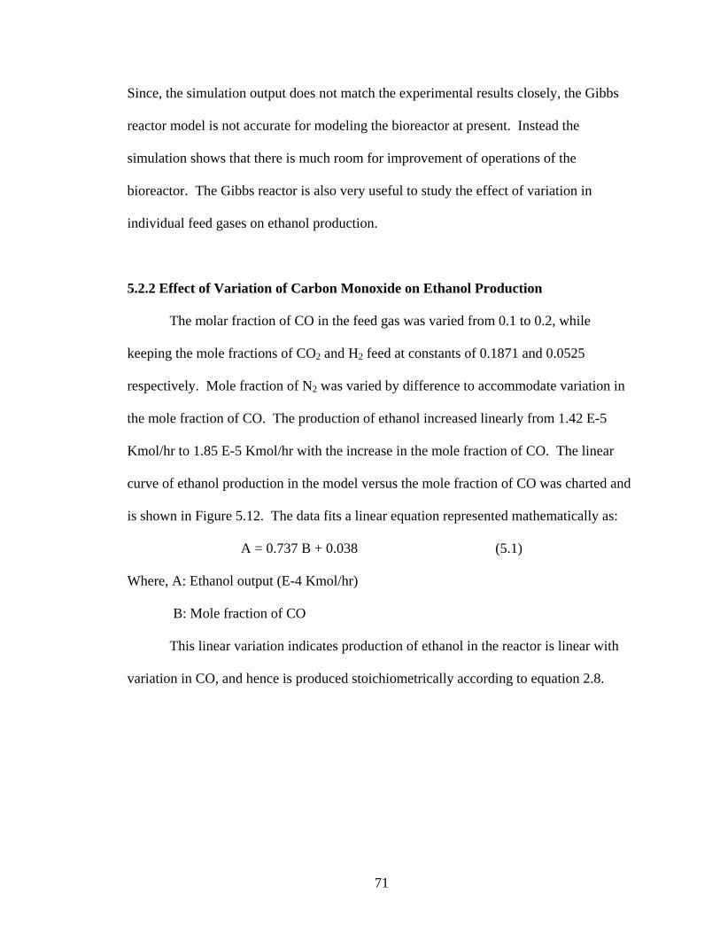
Since, the simulation output does not match the experimental results closely, the Gibbs
reactor model is not accurate for modeling the bioreactor at present. Instead the
simulation shows that there is much room for improvement of operations of the
bioreactor. The Gibbs reactor is also very useful to study the effect of variation in
individual feed gases on ethanol production.
5.2.2 Effect of Variation of Carbon Monoxide on Ethanol Production
The molar fraction of CO in the feed gas was varied from 0.1 to 0.2, while
keeping the mole fractions of CO2 and H2 feed at constants of 0.1871 and 0.0525
respectively. Mole fraction of N2 was varied by difference to accommodate variation in
the mole fraction of CO. The production of ethanol increased linearly from 1.42 E-5
Kmol/hr to 1.85 E-5 Kmol/hr with the increase in the mole fraction of CO. The linear
curve of ethanol production in the model versus the mole fraction of CO was charted and
is shown in Figure 5.12. The data fits a linear equation represented mathematically as:
A = 0.737 B + 0.038 (5.1)
Where, A: Ethanol output (E-4 Kmol/hr)
B: Mole fraction of CO
This linear variation indicates production of ethanol in the reactor is linear with
variation in CO, and hence is produced stoichiometrically according to equation 2.8.
71
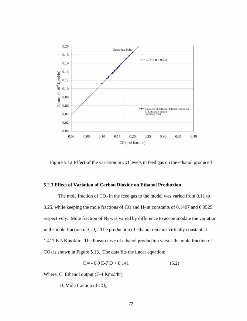
A = 0.7372 B + 0.038
0.00
0.02
0.04
0.06
0.08
0.10
0.12
0.14
0.16
0.18
0.20
0.00 0.05 0.10 0.15 0.20 0.25 0.30 0.35 0.40
CO (mol fraction)
Etha
nol (
x 10
-4 K
mol
/hr)
Bioreactor simulation - Ethanol ProductionVs CO Levels in feedOperating Point
Operating Point
Figure 5.12 Effect of the variation in CO levels in feed gas on the ethanol produced
5.2.3 Effect of Variation of Carbon Dioxide on Ethanol Production The mole fraction of CO2 in the feed gas to the model was varied from 0.11 to
0.25, while keeping the mole fractions of CO and H2 at constants of 0.1407 and 0.0525
respectively. Mole fraction of N2 was varied by difference to accommodate the variation
in the mole fraction of CO2. The production of ethanol remains virtually constant at
1.417 E-5 Kmol/hr. The linear curve of ethanol production versus the mole fraction of
CO2 is shown in Figure 5.13. The data fits the linear equation:
C = - 6.0 E-7 D + 0.141 (5.2)
Where, C: Ethanol output (E-4 Kmol/hr)
D: Mole fraction of CO2
72
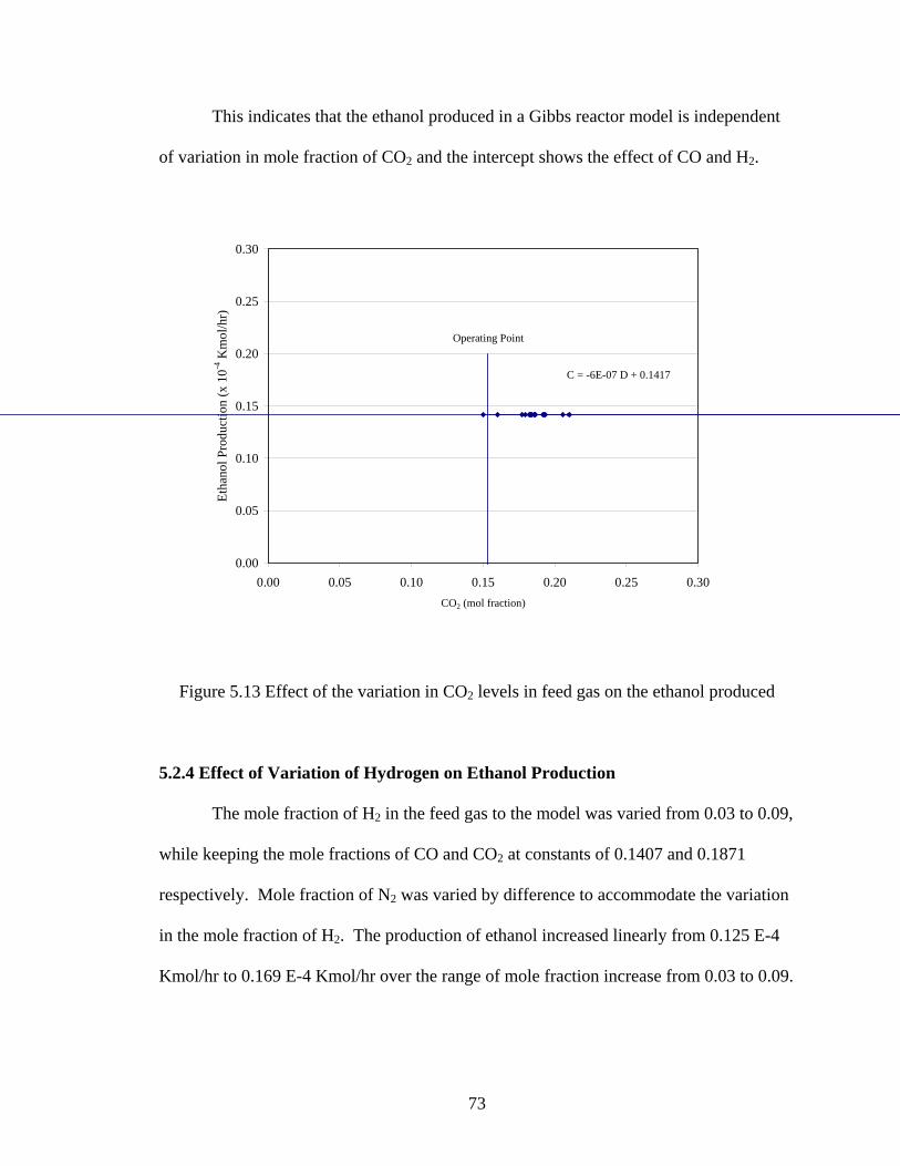
This indicates that the ethanol produced in a Gibbs reactor model is independent
of variation in mole fraction of CO2 and the intercept shows the effect of CO and H2.
0.00
0.05
0.10
0.15
0.20
0.25
0.30
0.00 0.05 0.10 0.15 0.20 0.25 0.30CO2 (mol fraction)
Etha
nol P
rodu
ctio
n (x
10-4
Km
ol/h
r)
C = -6E-07 D + 0.1417
Operating Point
Figure 5.13 Effect of the variation in CO2 levels in feed gas on the ethanol produced
5.2.4 Effect of Variation of Hydrogen on Ethanol Production
The mole fraction of H2 in the feed gas to the model was varied from 0.03 to 0.09,
while keeping the mole fractions of CO and CO2 at constants of 0.1407 and 0.1871
respectively. Mole fraction of N2 was varied by difference to accommodate the variation
in the mole fraction of H2. The production of ethanol increased linearly from 0.125 E-4
Kmol/hr to 0.169 E-4 Kmol/hr over the range of mole fraction increase from 0.03 to 0.09.
73

The variation in ethanol produced versus the variation in mole fraction in H2 is shown in
Figure 5.14.
The data fits the linear equation:
E = 0.737 F + 0.103 (5.3)
Where, E: Ethanol output (E-4 Kmol/hr)
F: Mole fraction of H2
This indicates that the ethanol production in a Gibbs reactor model is in linear
variance with a variation in the mole fraction of H2, and hence it is produced
stoichiometrically in a single reaction given by equation 2.9.
E = 0.7373 F + 0.103
0.10
0.11
0.12
0.13
0.14
0.15
0.16
0.17
0.18
0.19
0.20
0.00 0.02 0.04 0.06 0.08 0.10 0.12 0.14
H2 (mol fraction)
Etha
nol p
rodu
ctio
n (x
10-4
Km
ol/h
r)
Operating Point
Figure 5.14 Effect of the variation in H2 levels in feed gas on the ethanol produced
74
When equations 5.1, 5.2 and 5.3 are observed together, the linear variation in
equation 5.1 and equation 5.3 shows that the conversion of CO and H2 to form ethanol is
stoichiometrically similar. The intercept of equation 5.2 indicates that when no CO2 is
present in the reactor model, there is a production of 0.141 E-4 Kmol/hr of ethanol. The
intercepts of equation 5.1 and equation 5.3 add up to 0.141 E-4 Kmol/hr, which shows
that when CO2 is absent in the model, the net ethanol produced is due to the combined
individual effects of CO and H2. This validates the presence of a single reaction in the
reactor which is responsible for production of ethanol, in a Gibbs reactor model. This
reaction is a summation of equation 2.8 and equation 2.9, which can be represented as:
6 CO + 6 H2 2 C2H5OH + 2 CO2 (5.4)
This also shows that the simulated model can be used more accurately in prediction of
ethanol production if both the reactions are modeled individually in a reactor using Aspen
Plus™.
5.2.5 Effect of Variation of Media on Ethanol Production
The media feed to the reactor was increased from 1.0 E-6 Kg/sec to 5.0 E-5
Kg/sec while keeping the gas stream input at mole fractions of CO: 0.1407, CO2: 0.1871,
H2: 0.0525 and N2: 0.6197. The production of ethanol in the model increased from 1.748
E-7 Kg/sec to 1.763 E-7 Kg/sec on increasing the media input. This indicates that the
H2O is being consumed in the reactor according to equation 2.8. The mole fraction of
ethanol in the liquid output stream decreases exponentially due to dilution effects. A
75

chart of mole fractions of water and ethanol versus the media input to the reactor model is
shown in Figure 5.15.
y = 0.1982 Ln(x) + 0.6039
0.0
0.2
0.4
0.6
0.8
1.0
0.0 1.0 2.0 3.0 4.0 5.0 6.0
Media input to Reactor (x 10-5 Kg/sec)
Prod
uct s
tream
(mol
frac
)
Mol Fraction of Water
Mol Fraction of Ethanol
Operating Point
Operating Range
Operating Point
Figure 5.15 Effect of the variation in the media feed on the ethanol produced
5.2.6 Presence of Methane in the Model
In the model, when methane was defined as a possible product in the Gibbs
reactor mode, ethanol production was reduced drastically. In the absence of methane, the
base case model showed a production rate of ethanol of 2.149 E-7 Kg/sec. This is
reduced to 1.026 E-24 Kg/sec in the presence of 0.001 volume percent of CH4 in the feed
gas. An excessive amount of CH4 was produced in the model. This can be explained by
the thermodynamic stability of CH4 and preferential production of CH4 over ethanol. The
76

Gibbs reactor model assumes infinite reaction time and complete attainment of
equilibrium, which indicates that eventually most of the feed gases might get converted to
methane as the preferred product. For this reason, CH4 was excluded as an inlet or outlet
component for all bioreactor simulations using the Gibbs reactor model.
5.2.7 Base Case Simulation Output and Model Validation: Stoichiometric Reactor
A base case simulation was developed on the basis of input data from a standard
experimental run of the bioreactor in a laboratory set-up. The composition of the feed
gas stream and media stream are listed in Table 5.3. The reaction stoichiometry of
equation 2.8 and equation 2.9 were specified for the reactor model. The stoichiometric
conversions for both the reactions were varied simultaneously from 0.05 to 0.95 and
output results were matched to the experimental output. The output data from the model
at a conversion of 0.1 for both the reactions was found to closely fit the experimental
output. The results from the simulation are presented in Table 5.5 and compared with
experimental results.
The CO output from the model was at a rate of 1.944 E-8 Kmol/sec which is close
to the experimental output of 2.033 E-8 Kmol/sec. CO2 production in the model was
2.142 E-8 Kmol/sec which is close to the experimental production value of 2.162 E-8
Kmol/sec. H2 production in the model was 6.133 E-9 Kmol/sec which is close to the
experimental output value of 6.396 E-9 Kmol/sec. Ethanol production in the model was
2.182 E-8 Kg/sec which was higher than the experimental output of 4.38 E-9 Kg/sec. A
chart indicating the variation of output gases with the variation in E1 and E2 is shown in
Figure 5.16. A close fit of output data from the simulation indicates that the laboratory
77

set-up of the bioreactor is comparable to a stoichiometric reactor model working at 10%
efficiency.
Figure 5.16 Effect of variation in the stoichiometric conversions on the exit gas
composition
0
0.1
0.2
0.3
0.4
0 0.2 0.4 0.6 0.8
Stoichiometric Conversion
Mol
Fra
ctio
n 0.5
0.6
0.7
0.8
1
CO
CO2
H2
N2
78
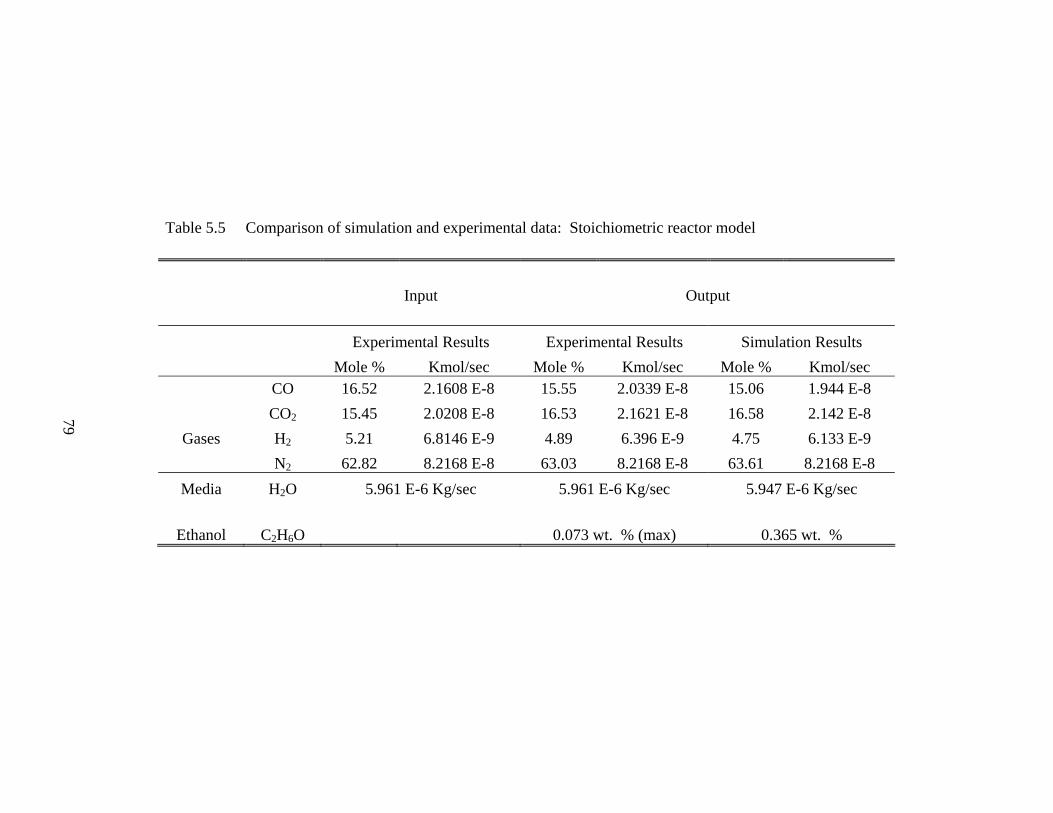
Table 5.5 Comparison of simulation and experimental data: Stoichiometric reactor model
Input Output Experimental Results Experimental Results Simulation Results Mole % Kmol/sec Mole % Kmol/sec Mole % Kmol/sec CO 16.52 2.1608 E-8 15.55 2.0339 E-8 15.06 1.944 E-8
CO2 15.45 2.0208 E-8 16.53 2.1621 E-8 16.58 2.142 E-8 Gases H2 5.21 6.8146 E-9 4.89 6.396 E-9 4.75 6.133 E-9
N2 62.82 8.2168 E-8 63.03 8.2168 E-8 63.61 8.2168 E-8 Media H2O 5.961 E-6 Kg/sec 5.961 E-6 Kg/sec 5.947 E-6 Kg/sec
Ethanol C2H6O 0.073 wt. % (max) 0.365 wt. %
79
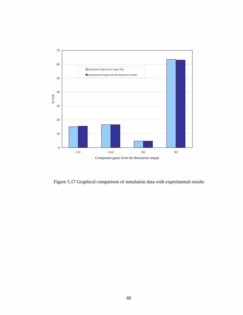
0
10
20
30
40
50
60
70
CO CO2 H2 N2
Component gases from the Bioreactor output
% V
ol
Simulation Output from Aspen Plus
Experimental Output from the Bioreactor studies
Figure 5.17 Graphical comparison of simulation data with experimental results
80

5.2.8 Effect of Stoichiometric Conversion on Ethanol Production In this analysis, stoichiometric conversions for reactions 2.8 and 2.9, defined as E1
and E2, were varied independently of each other to study their individual effects on
ethanol production as shown in Figure 5.20. A sensitivity tool was used to vary E1 while
keeping E2 at 0.1. The output mole fractions of CO, CO2, H2 and N2 were plotted against
E1, as shown in Figure 5.18. The production of ethanol increased linearly with an
increase in E1. The sensitivity analysis was run again by varying E2 while keeping E1 at
0.1. The variation in output mole fractions of CO, CO2, H2 and N2 were plotted against
E2 and are depicted in Figure 5.19. The production of ethanol increased linearly with an
increase in E2, although with a lesser influence when compared to variation in E1. A
comparison between variations in both E1 and E2 and their effect on ethanol production is
shown in Figure 5.20.
81

0
0.1
0.2
0.3
0.4
0.5
0.6
0.7
0.8
0 0.2 0.4 0.6 0.8 1
Stoichiometric Conversion (E1)
Mol
. Fra
ctio
n
CO
CO2
H2
N2
E2 = 0.1
Figure 5.18 Effect of variation in the stoichiometric conversion (E1) on the exit gas
composition
82

0
0.1
0.2
0.3
0.4
0.5
0.6
0.7
0.8
0 0.2 0.4 0.6 0.8 1
Stoichiometric Conversion (E2)
Mol
Fra
ctio
n
COCO2H2N2
E1 = 0.1
Figure 5.19 Effect of variation in the stoichiometric conversion (E2) on the exit gas
composition
83

y = 0.8453 x + 0.2735
y = 2.7349 x + 0.0846
0.0
0.5
1.0
1.5
2.0
2.5
3.0
0 0.2 0.4 0.6 0.8 1Stoichiometric Conversion
Etha
nol O
utpu
t (w
t. %
)
Ethanol Output Vs. E2 Ethanol Output Vs. E1
Figure 5.20 Effect of variation in the stoichiometric conversions on the ethanol produced
5.2.9 Energy Balance for the Bioreactor Model
The energy balance for the Gibbs reactor model of the bioreactor shows a net heat
duty of – 0.7616 Kcal/hr for the base case. The energy balance for the stoichiometric
reactor model shows a net heat duty of 0.4629 Kcal/hr for the base case.
84
CHAPTER 6
CONCLUSIONS AND RECOMMENDATIONS
6.1 Conclusions
A pilot plant gasifier and a laboratory bioreactor at Oklahoma State University,
used to study the production of ethanol from switchgrass, were simulated in this study.
Aspen Plus™, a commercial process simulation software was used to develop simulation
models for the gasifier and the bioreactor, based on experimental parameters of operation.
The results described in this thesis, based on the Aspen Plus™ simulations can be used to
help reduce time consuming and expensive experimentation. The conclusions from the
study are discussed in the following sections.
6.1.1 Gasifier simulation
The gasifier was modeled using a Gibbs free energy minimization model in Aspen
PlusTM. The Gibbs model is based on thermodynamic equilibrium and gave results which
were close to the experimental values. Sensitivity was tested based on varying operation
parameters and the results from the model were similar to other studies on gasifier
performance found in the literature. Since the model is an equilibrium model, it cannot
be used for scale up and design purposes. However, the sensitivity studies can be used to
85
predict the performance of the gasifier at unknown operating conditions. This work can
be used to:
• Predict exhaust composition of syngas at various biomass feed rates
• Predict exhaust gas composition at various moisture contents associated
with the biomass
• Predict exhaust composition of syngas and individual flowrates of gases
at various gasification temperatures
• Predict composition and variation of trace hydrocarbons produced during
biomass gasification
• Predict effect of the Air Fuel ratio on the syngas composition and the
individual gas flowrates
• Predict effect of the Equivalence Ratio on the syngas composition
• Predict effect of the Equivalence Ratio on the syngas at 750 ºC, 815 ºC,
875 ºC and 925 ºC.
Some of the chief conclusions are:
1) The base case simulation results show a 10.55 Kg/hr production of CO, which
is 64.1% greater than the experimental production of 6.43 Kg/hr. This indicates a
theoretical higher potential for CO production in the gasifier.
2) The base case simulation results show a 0.696 Kg/hr production of H2 which is
more than four times greater than the experimental production of 0.16 Kg/hr H2.
This indicates a theoretical higher potential for H2 production in the gasifier.
3) Production of CO drops with an increase in the moisture content of biomass.
Hence, preparation and drying of biomass are critical for greater CO production.
86

4) The Equivalence Ratio was found to be the most influential variable on syngas
composition. An increase in the ER leads to a decrease in the production of CO
and H2.
6.1.2 Bioreactor simulation
The bioreactor model was modeled in Aspen PlusTM using two approaches, an
equilibrium approach and a stoichiometric approach. The equilibrium model was based
on Gibbs free energy minimization and was used to estimate the maximum theoretical
ethanol production. The results from the equilibrium model were much greater than the
observed values from the laboratory studies, indicating that there is a potential for great
improvement in the laboratory reactor. The equilibrium model was also used to study the
sensitivity of the bioreactor model to changes in the composition of syngas. This work
can be used to benchmark the production of ethanol possible out of the present reactor set
up. The simulation studies can also be used to:
• Predict the maximum ethanol production possible
• Study the effect of changes in the feed syngas composition on the ethanol
produced
The stoichiometric model in Aspen Plus™ was based on the two main reactions
occurring in the bioreactor. The results from the model were close to the experimental
results. The stoichiometric conversions were varied for the two main reactants in the
reactions simultaneously and individually to study the effect on ethanol production and
output gas composition. These results can be used to:
• Predict the ethanol production at various stoichiometric conversions of
the two combined reactions
87
• Predict the influence of the stoichiometric conversion of the combined
reactions on the output gas composition from the bioreactor
• Predict the ethanol production with variation in individual stoichiometric
conversion of each reaction
• Predict the influence of stoichiometric conversion of each reaction
individually on the output gas composition from the bioreactor
Some of the chief conclusions are:
1) The base case analysis using the gibbs reactor model shows an ethanol
production of 3.56% by weight which is much greater than the experimental
production of 0.073% by weight. This shows that there is room for improvement
in the ethanol production in laboratory studies.
2) A higher input of CO and H2 results in an increase in the ethanol production in
the sensitivity analysis. This indicates that we can increase the production of
ethanol by increasing the composition of CO and H2 in the syngas. This could be
achieved by steam gasification.
3) A higher ethanol production results from increasing the stoichiometric
conversion in the stoichiometric reactor model. This indicates that CO and H2 are
not completely utilized in the bioreactor for ethanol production and we can
improve the consumption of CO and H2 further.
88

6.2 Recommendations for future work
The reactor models developed in this work were built in Aspen Plus™ and are
generic in nature. Although the gasifier model gives accurate predictions of gasifier
performance at unknown operation parameter ranges, it cannot be used for scale up or
design purposes. For scale up of the gasifier, kinetic data on biomass gasification is
required. With the help of kinetic data, a gasifier model could be developed in Aspen
Plus™ using the kinetic reactor, which would be useful for scaling up the gasifier for
industry level production.
For a precise fit of the reactor model for the bioreactor simulation, kinetic data and
biochemical equations governing the production of ethanol are required and need to be
programmed into Aspen Plus™ using FORTRAN subroutines. Future work on
bioreactor simulations could include user defined subroutines in Aspen Plus™ for local
use and a better fit of the model to laboratory experimentation for syngas conversion
using P7. With the use of kinetic data, this reactor model could be used for scale up
purposes.
A distillation model is required for complete simulation of the entire process of
conversion of switchgrass to ethanol. An integrated design of the entire plant at an
industry level of production is needed to successfully study the performance of the entire
plant. An optimization study aimed at optimizing performance of the gasifier, bioreactor
and distillation units is required as well as an optimization for the entire process as an
integrated plant. In such an optimization study, the amount of ethanol produced could be
used as an objective function and the effects of process parameters on the objective
89

function could be analyzed, thus developing a generalized correlation for the objective
function.
90

REFERENCES
Ahmed, A., Lewis, R. S. (2005). “Effects of Biomass-Generated Syngas Constituents on Cell Growth, Product Distribution and Hydrogenase Activity of Clostridium carboxidivorans P7T.” Biotechnology and Bioengineering, Paper under review.
Aspen Tech 12.1 User Manuals (2003), Aspen Technology: Cambridge, Massachusetts. Belgiorno, V., De Feo, G., Rocca, C. D. and Napoli, R. M. A. (2003). “Energy from
gasification of solid wastes.” Waste management, 23, 1-15. Bettagli, N., Desideri, U. and Fiaschi, D. (1995). “A biomass combustion – gasification
model: Validation and Sensitivity Analysis.” Journal of Energy Resources Technology, 117, 329-336.
Beukens, A. G. and Schoeters, J. G. (1989). “Modeling of biomass gasification.”
Fundamentals of thermochemical biomass conversion, Overend, R. P., Milne, T.A. and Mudge, L.K (eds.), Elsevier: New Hampshire, England, pp 619-689.
Bilodeau, J. F., Therien, N., Proulx, P., Czernik, S. and Chornet, E. (1993). “A
mathematical model of fluidized bed biomass gasification.” The Canadian Journal of Chemical Engineering, 71, 549-557.
Bingyan, X., Chuangzhi, W., Zhengfen, L. and Guang, Z. Xi (1992). “Kinetic study on
biomass gasification.” Solar Energy, 49, 3, 199-204. Bridgewater, A. V. (2003). “Renewable fuels and chemicals by thermal processing of
biomass.” Chemical Engineering Journal, 91, 87-102. Bridgewater, A.V., Double, J. M. and Smith, E. L. (1989). “Computer Modeling of
Fluidized bed gasification.” Gasification and Pyrolysis, Ferrero, G. L., Maniatis, K. and Beukens, A. (eds.), Elsevier Applied Science: New York, pp 651-655.
Carlson, E. E. (1996). “Don’t gamble with physical properties for simulations.” Chemical
Engineering Progress, October 1996, 35-46. Cateni, B. G., Bellmer, D. D., Huhnke, R. L., Lelo, M. M. and Bowser, T. J. (2000).
“Recirculation in a fluidized bed gasifier to minimize oxygen content in synthesis gas from biomass.” ASAE Paper No. 006033, July 2000.
91

Datar, R. P. (2003). Anaerobic fermentation of biomass generated producer gas to ethanol. Ph.D dissertation, Oklahoma State University, Stillwater, Oklahoma.
Datar, R. P., Shenkman, R. M., Cateni, B. G., Huhnke, R. L. and Lewis, R. S. (2004).
“Fermentation of biomass-generated producer gas to ethanol.” Biotechnology and Bioengineering, 86, 5, 587-594.
Esplin, G.J., Fung, D. P. C. and Hsu, C. C. (1986). “A comparison of the Energy and
Product distribution from biomass gasifiers.” The Canadian Journal of Chemical Engineering, 64, 651-662.
Furman, A. H., Kimura, S. G., Ayala, R. E. and Joyce, J. F. (1993). “Biomass
Gasification Pilot Plant Study.” EPA Project Summary, EPA/600/SR-93/170. Greene, D. L and Schafer, A. (2003). “Reducing green house gas emissions from U.S
transportation.” Prepared for the Pew Center on Global Climate Change, May 2003, 1-80.
Hatt, B. W., Iredale, P. J., Irlam, G. A., Shand, R. N., Sheena, H. H. and Smith, E. L.
(1985). “Research on the gasification of biomass at the University of Aston in Birmingham.” Fundamental of Thermochemical Biomass Conversion, Overend, R. P, Milne, T.A. and Mudge, L. K. (eds.), Elsevier Applied Science Publishers: New Hampshire, England, pp 473-484.
Hohenstein, W. G. and Wright, L. L. (1994). “Biomass energy production in the United
States: An overview.” Biomass and Bioenergy, 6, 3, 161-173. Kalil, S. J., Maugeri, F. and Rodrigues, M. I. (2000). “Response surface analysis and
simulation as a tool for bioprocess design and optimization.” Process Biochemistry, 35, 539-550.
Kinoshita, M. C., Wang, Y. and Takahashi, P. K. (1991). “Chemical equilibrium
computations for gasification of biomass to produce methanol.” Energy Sources, 13, 361-368.
Klasson, K. T., Ackerson, M. D., Clausen, E. C. and Gaddy, J. L. (1992). “Bioconversion
of synthesis gas into liquid or gaseous fuels.” Enzyme Microbial Technology, 14, 602-608.
Klasson, K. T., Elmore, B. B., Vega, J. L., Ackerson, M. D., Clausen, E. C. and Gaddy, J.
L. (1990). “Biological production of liquid fuels from synthesis gas.” Applied Biochemistry and Biotechnology, 24-25, 857-873.
Lee, J. M., Pollard, J. F. and Coulman, G. A. (1983). “Ethanol fermentation with cell
recycling: Computer simulation.” Biotechnology and Bioengineering, 25, 497-511.
92

Luyben, W. L. (2004). “Use of Dynamic Simulation to converge complex process flowsheets.” Chemical Engineering Education, Spring 2004, 142-149.
Lynd, L. R., Cushman, J. H., Nichols, R. J. and Wyman, C. E. (1991). “Fuel Ethanol
from Cellulosic Biomass.” Science, 251, 1318-1323. McKendry, P. (2002a). “Energy production from biomass (part 1): Overview of
biomass.” Bioresource Technology, 83, 37-46. McKendry, P. (2002b). “Energy production from biomass (part 2): Conversion
technologies.” Bioresource Technology, 83, 47-54. McLaughlin, S. B. and Walsh, M. E. (1998). “Evaluating environmental consequences of
producing herbaceous crops for bioenergy.” Biomass and Bioenergy, 14, 4, 317-324. Mussati, M., Aguirre, P. and Scenna, N. J. (1998). “Modeling of real biological reactors
for the treatment of complex substrates: Dynamic Simulation.” Computers and Chemical Engineering, 22, Supplement, S723-S726.
Nadim, F., Zack, P., Hoag, George E. and Liu, S. (2001). “United States experience with
gasoline additives” Energy Policy, 29, 1-5. Narvaez, I., Orio, A., Aznar, M. P. and Corella, J. (1996). “Biomass gasification with air
in an atmospheric bubbling fluidized bed. Effect of six operational variables on the quality of produced raw gas.” Industrial and Engineering Chemistry Research, 35, 2110-2120.
Natarajan, E., Nordin, A. and Rao, A. N. (1998). “Overview of combustion and
gasification of rice husk in fluidized bed reactors.” Biomass and Bioenergy, 14, 5/6, 533-546.
Nihtila, M. T., Tervo, J. and Kaipio, J. P. (1997). “Simulation of a nonlinear distributed
parameter bioreactor by FEM approach.” Simulation Practice and Theory, 5, 199-216. Pascal, F., Dagot, C., Pingaud, H., Corriou, J. P., Pons, M. N. and Engasser, J. M. (1995).
“Modeling of an Industrial Alcohol Fermentation and Simulation of the plant by a process simulator.” Biotechnology and Bioengineering, 46, 202-217.
Paul, J. K. (1979). Ethyl Alcohol production and its use as a motor fuel, Noyes Data:
Park Ridge, New Jersey, pp 1-2. Pimentel, D. and Patzek, T. W. (2005). “Ethanol production using corn, switchgrass, and
wood: biodiesel production using soybean and sunflower.” Natural Resources Research, 14, 1, 65-76.
93

Nihtila, M. T., Tervo, J. and Kaipio, J. P. (1997). “Simulation of nonlinear distributed parameter bioreactor by FEM approach.” Simulation practice and theory, 5, 199-216.
Rajagopalan, S. (2001). Microbial conversion of syngas to ethanol. Ph.D dissertation,
Oklahoma State University, Stillwater, Oklahoma. Rajagopalan, S., Datar, R. P. and Lewis, R. S. (2002). “Formation of ethanol from carbon
monoxide via a new microbial catalyst.” Biomass and Bioenergy, 23, 487-493. Raman, R. (1985). Chemical Process Computations, Elsevier Applied Science Publishers:
London and New York, pp 7-8. Reed, T. B. (1981). Biomass Gasification: Principles and Technology, Noyes Data
Corporation: New Jersey. Renewable Fuels Association. (2005). “Ethanol Industry Outlook 2005: Homegrown for
the Homeland”, 1-15. Richard, J. R., Cathonnet, M. and Rouan, J. P. (1989). “Gasification of charcoal:
Influence of water vapor.” Fundamentals of thermochemical biomass conversion, Overend, R. P., Milne, T. A. and Mudge, L. K (eds.), Elsevier: New Hampshire, London. pp 589-599.
Sanderson, M. S., Reed, R. L., McLaughlin, S. B., Wullschleger, S. D., Conger, B. V.,
Parrish, D. J., Wolf, D. D., Taliaferro, C., Hopkins, A. A., Ocumpaugh, W. R., Hussey, M. A., Read, J. C. and Tischler, C. R. (1996). “Switchgrass as a sustainable bioenergy crop.” Bioresource Technology, 56, 83-93.
Schuster, G., Loffler, G., Weigl, K. and Hofbauer, H. (2001). “Biomass steam
gasification – an extensive parametric modeling study.” Bioresource Technology, 77, 71-79.
Wang, Y. and Kinoshita, C. M. (1992). “Experimental analysis of biomass gasification
with steam and oxygen.” Solar Energy, 49, 3, 153-158. Wang, Y. and Kinoshita, C. M. (1993). “Kinetic model of biomass gasification.” Solar
Energy, 51, 1, 19-25. Wang, M., Saricks, C. and Santini, D. (1999). “Greenhouse gas emissions of fuel ethanol
produced from corn and cellulosic biomass.” EM: Air and waste management association’s magazine for environmental managers, October, 17-25.
Wood, H. G., Ragsdale, S. W. and Pezacka, E. (1986). “A new pathway of autotrophic
growth utilizing carbon monoxide or carbon dioxide and hydrogen.” Biochemistry International, 12, 3, 421-440.
94

Wooley, R. J. and Ibsen, K. N. (2000). Rapid evaluation of research proposals using Aspen Plus™. Presentation at AspenWorld 2000, Orlando, FL, Feb 2000.
Watkinson, A. P., Lucas, J. P. and Lim, C. J. (1991). “A prediction of performance of
commercial coal gasifiers.” Fuel, 70, April, 1991. Yacobucci, Brent D. and Womach, Jasper (2004). “Fuel Ethanol: Background and public
policy issues.” CRS Report for Congress, December 2004.
95

APPENDIX A
SIMULATION DATA TABLES
96

A.1 Complete list of exhaust gas components from the gasifier
Component Flowrate (Kg/hr) C 4.8061 E-27 H2 0.6966 O2 1.9237 E-17 N2 23.25
H2O 3.5437 CO 10.5504 CO2 9.7278 CH4 0.4016 E-3 NO 4.4215 E-12 NO2 2.4309 E-22 C2H2 1.1908 E-10 C2H4 1.9396 E-9 C2H6 2.4551 E-10
97

98
A.2 Simulation data from the gasifier model for biomass sensitivity analysis
Biomass Input Product Gases
H2 N2 CO CO2 CH4 H2O (Kg/hr) (Kg/hr) (Kg/hr) (Kg/hr) (Kg/hr) (Kg/hr) (Kg/hr) 12.000 0.339 23.205 5.116 9.862 0.000 3.608 12.750 0.387 23.211 5.838 9.846 0.000 3.598 13.500 0.434 23.217 6.561 9.829 0.000 3.589 14.250 0.482 23.223 7.283 9.812 0.000 3.580 15.000 0.529 23.229 8.006 9.795 0.001 3.571 15.750 0.576 23.235 8.729 9.777 0.001 3.562 16.500 0.624 23.241 9.452 9.759 0.001 3.553 17.250 0.671 23.247 10.175 9.741 0.001 3.544 17.640 0.696 23.250 10.551 9.732 0.001 3.540 18.000 0.718 23.253 10.898 9.723 0.002 3.536 18.750 0.766 23.259 11.621 9.705 0.002 3.528 19.500 0.813 23.265 12.344 9.687 0.002 3.519 20.250 0.860 23.271 13.067 9.668 0.003 3.511 21.000 0.907 23.277 13.790 9.650 0.003 3.503 21.750 0.955 23.283 14.513 9.631 0.004 3.495 22.500 1.002 23.288 15.236 9.613 0.005 3.487 23.250 1.049 23.294 15.958 9.594 0.005 3.479 24.000 1.096 23.300 16.681 9.576 0.006 3.471
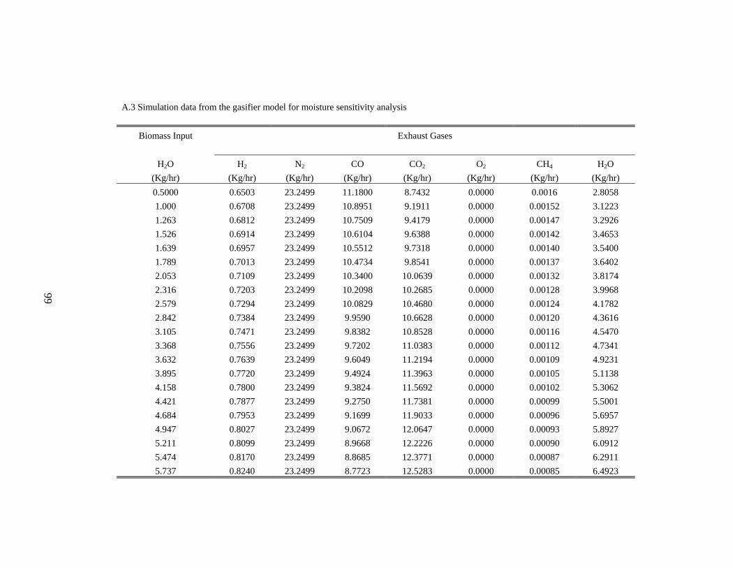
99
A.3 Simulation data from the gasifier model for moisture sensitivity analysis
Biomass Input Exhaust Gases
H2O H2 N2 CO CO2 O2 CH4 H2O (Kg/hr)
(Kg/hr) (Kg/hr) (Kg/hr) (Kg/hr) (Kg/hr) (Kg/hr) (Kg/hr)
0.5000 0.6503 23.2499 11.1800 8.7432 0.0000 0.0016 2.80581.000
0.6708 23.2499 10.8951 9.1911 0.0000 0.00152 3.12231.263 0.6812 23.2499 10.7509 9.4179 0.0000 0.00147 3.29261.526 0.6914 23.2499 10.6104 9.6388 0.0000 0.00142 3.46531.639 0.6957 23.2499 10.5512 9.7318 0.0000 0.00140 3.54001.789 0.7013 23.2499 10.4734 9.8541 0.0000 0.00137 3.64022.053 0.7109 23.2499 10.3400 10.0639 0.0000 0.00132 3.81742.316 0.7203 23.2499 10.2098 10.2685 0.0000 0.00128 3.99682.579 0.7294 23.2499 10.0829 10.4680 0.0000 0.00124 4.17822.842 0.7384 23.2499 9.9590 10.6628 0.0000 0.00120 4.36163.105 0.7471 23.2499 9.8382 10.8528 0.0000 0.00116 4.54703.368 0.7556 23.2499 9.7202 11.0383 0.0000 0.00112 4.73413.632 0.7639 23.2499 9.6049 11.2194 0.0000 0.00109 4.92313.895 0.7720 23.2499 9.4924 11.3963 0.0000 0.00105 5.11384.158 0.7800 23.2499 9.3824 11.5692 0.0000 0.00102 5.30624.421 0.7877 23.2499 9.2750 11.7381 0.0000 0.00099 5.50014.684 0.7953 23.2499 9.1699 11.9033 0.0000 0.00096 5.69574.947 0.8027 23.2499 9.0672 12.0647 0.0000 0.00093 5.89275.211 0.8099 23.2499 8.9668 12.2226 0.0000 0.00090 6.09125.474 0.8170 23.2499 8.8685 12.3771 0.0000 0.00087 6.29115.737 0.8240 23.2499 8.7723 12.5283 0.0000 0.00085 6.4923
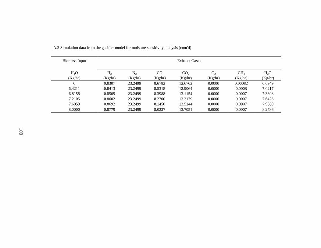
100
A.3 Simulation data from the gasifier model for moisture sensitivity analysis (cont'd)
Biomass Input Exhaust Gases
H2O H2 N2 CO CO2 O2 CH4 H2O (Kg/hr)
(Kg/hr) (Kg/hr) (Kg/hr) (Kg/hr) (Kg/hr) (Kg/hr) (Kg/hr)
6 0.8307 23.2499 8.6782 12.6762 0.0000 0.00082 6.69496.4211
0.8413 23.2499 8.5318 12.9064 0.0000 0.0008 7.02176.8158 0.8509 23.2499 8.3988 13.1154 0.0000 0.0007 7.33087.2105 0.8602 23.2499 8.2700 13.3179 0.0000 0.0007 7.64267.6053 0.8692 23.2499 8.1450 13.5144 0.0000 0.0007 7.95698.0000 0.8779 23.2499 8.0237 13.7051 0.0000 0.0007 8.2736

101
A.4 Simulation data from the gasifier model for temperature sensitivity analysis: mass basis
TEMP H2 N2 O2 H2O CO CO2 CH4 NO NO2
(K) (Kg/hr) (Kg/hr) (Kg/hr)
(Kg/hr) (Kg/hr) (Kg/hr) (Kg/hr) (Kg/hr) (Kg/hr)873 0.663 23.250 0.000 0.000 7.219 13.469 0.545 0.000 0.000898
0.714 23.250 0.000 0.000 8.158 12.644 0.309 0.000 0.000923 0.742 23.250 0.000 0.000 8.835 11.995 0.157 0.000 0.000948 0.750 23.250 0.000 0.000 9.296 11.496 0.075 0.000 0.000973 0.746 23.250 0.000 0.000 9.621 11.095 0.035 0.000 0.000998 0.738 23.250 0.000 0.000 9.873 10.750 0.017 0.000 0.000
1023 0.727 23.250 0.000 0.000 10.086 10.439 0.008 0.000 0.0001048 0.715 23.250 0.000 0.000 10.276 10.152 0.004 0.000 0.0001073 0.703 23.250 0.000 0.000 10.450 9.883 0.002 0.000 0.0001088 0.697 23.250 0.000 0.000 10.550 9.728 0.001 0.000 0.0001098 0.692 23.250 0.000 0.000 10.614 9.630 0.001 0.000 0.0001123 0.681 23.250 0.000 0.000 10.767 9.389 0.001 0.000 0.0001148 0.671 23.250 0.000 0.000 10.913 9.162 0.000 0.000 0.0001173 0.661 23.250 0.000 0.000 11.050 8.946 0.000 0.000 0.000
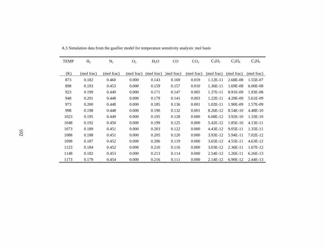
102
A.5 Simulation data from the gasifier model for temperature sensitivity analysis: mol basis
TEMP H2 N2 O2 H2O CO CO2 C2H2 C2H4 C2H6
(K) (mol frac) (mol frac) (mol frac) (mol frac) (mol frac) (mol frac) (mol frac) (mol frac) (mol frac)
873 0.182 0.460 0.000 0.143 0.169 0.019 1.12E-11 2.68E-08 1.55E-07898
0.193 0.453 0.000 0.159 0.157 0.010 1.36E-11 1.69E-08 6.00E-08923 0.199 0.449 0.000 0.171 0.147 0.005 1.37E-11 8.91E-09 1.93E-08948 0.201 0.448 0.000 0.179 0.141 0.003 1.22E-11 4.20E-09 5.61E-09973 0.200 0.448 0.000 0.185 0.136 0.001 1.02E-11 1.90E-09 1.57E-09998 0.198 0.448 0.000 0.190 0.132 0.001 8.26E-12 8.54E-10 4.48E-10
1023 0.195 0.449 0.000 0.195 0.128 0.000 6.68E-12 3.92E-10 1.33E-101048 0.192 0.450 0.000 0.199 0.125 0.000 5.42E-12 1.85E-10 4.13E-111073 0.189 0.451 0.000 0.203 0.122 0.000 4.43E-12 9.05E-11 1.35E-111088 0.188 0.451 0.000 0.205 0.120 0.000 3.93E-12 5.94E-11 7.02E-121098 0.187 0.452 0.000 0.206 0.119 0.000 3.65E-12 4.55E-11 4.63E-121123 0.184 0.452 0.000 0.210 0.116 0.000 3.03E-12 2.36E-11 1.67E-121148 0.182 0.453 0.000 0.213 0.114 0.000 2.54E-12 1.26E-11 6.26E-131173 0.179 0.454 0.000 0.216 0.111 0.000 2.14E-12 6.90E-12 2.44E-13
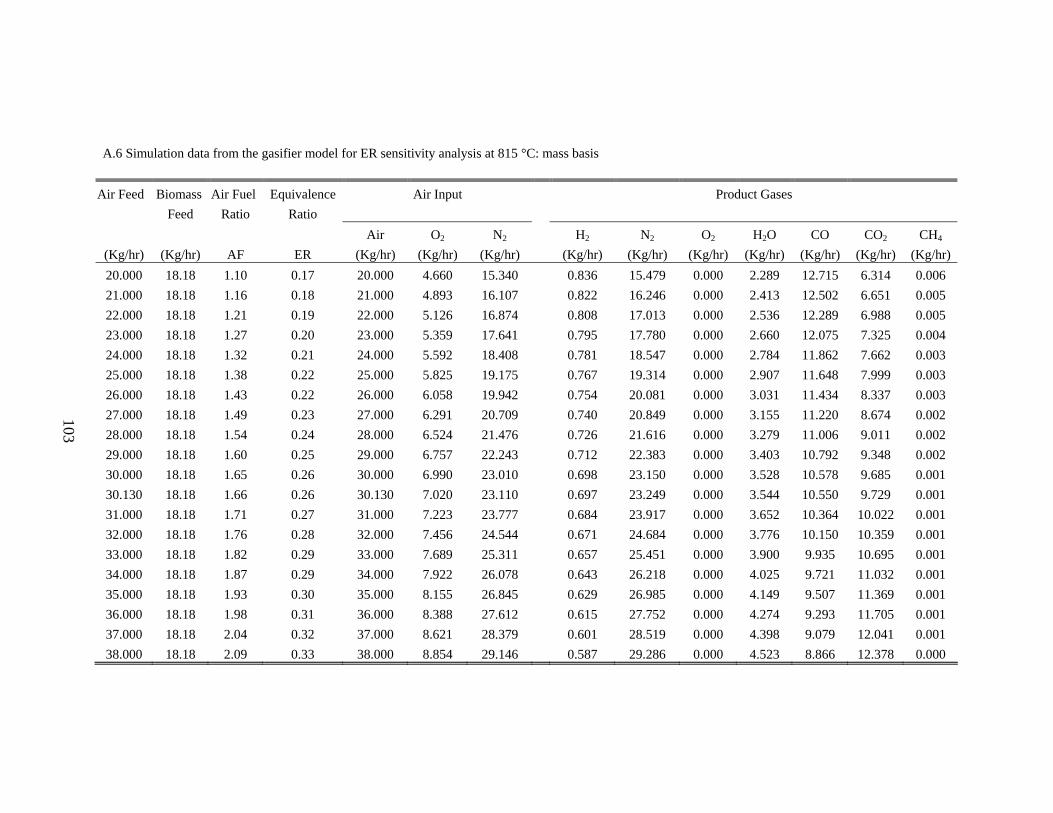
103
A.6 Simulation data from the gasifier model for ER sensitivity analysis at 815 °C: mass basis
Air Feed Biomass Air Fuel Equivalence Air Input Product Gases H
Feed Ratio Ratio Air O2 N2 2 N2 O2 H2O CO CO2 CH4
(Kg/hr)
(Kg/hr) AF ER (Kg/hr) (Kg/hr) (Kg/hr) (Kg/hr) (Kg/hr) (Kg/hr) (Kg/hr) (Kg/hr) (Kg/hr) (Kg/hr)20.000 18.18 1.10 0.17 20.000 4.660 15.340 0.836 15.479 0.000 2.289 12.715 6.314 0.00621.000
18.18 1.16 0.18 21.000 4.893 16.107 0.822 16.246 0.000 2.413 12.502 6.651 0.00522.000 18.18 1.21 0.19 22.000 5.126 16.874 0.808 17.013 0.000 2.536 12.289 6.988 0.00523.000 18.18 1.27 0.20 23.000 5.359 17.641 0.795 17.780 0.000 2.660 12.075 7.325 0.00424.000 18.18 1.32 0.21 24.000 5.592 18.408 0.781 18.547 0.000 2.784 11.862 7.662 0.00325.000 18.18 1.38 0.22 25.000 5.825 19.175 0.767 19.314 0.000 2.907 11.648 7.999 0.00326.000 18.18 1.43 0.22 26.000 6.058 19.942 0.754 20.081 0.000 3.031 11.434 8.337 0.00327.000 18.18 1.49 0.23 27.000 6.291 20.709 0.740 20.849 0.000 3.155 11.220 8.674 0.00228.000 18.18 1.54 0.24 28.000 6.524 21.476 0.726 21.616 0.000 3.279 11.006 9.011 0.00229.000 18.18 1.60 0.25 29.000 6.757 22.243 0.712 22.383 0.000 3.403 10.792 9.348 0.00230.000 18.18 1.65 0.26 30.000 6.990 23.010 0.698 23.150 0.000 3.528 10.578 9.685 0.00130.130 18.18 1.66 0.26 30.130 7.020 23.110 0.697 23.249 0.000 3.544 10.550 9.729 0.00131.000 18.18 1.71 0.27 31.000 7.223 23.777 0.684 23.917 0.000 3.652 10.364 10.022 0.00132.000 18.18 1.76 0.28 32.000 7.456 24.544 0.671 24.684 0.000 3.776 10.150 10.359 0.00133.000 18.18 1.82 0.29 33.000 7.689 25.311 0.657 25.451 0.000 3.900 9.935 10.695 0.00134.000 18.18 1.87 0.29 34.000 7.922 26.078 0.643 26.218 0.000 4.025 9.721 11.032 0.00135.000 18.18 1.93 0.30 35.000 8.155 26.845 0.629 26.985 0.000 4.149 9.507 11.369 0.00136.000 18.18 1.98 0.31 36.000 8.388 27.612 0.615 27.752 0.000 4.274 9.293 11.705 0.00137.000 18.18 2.04 0.32 37.000 8.621 28.379 0.601 28.519 0.000 4.398 9.079 12.041 0.00138.000 18.18 2.09 0.33 38.000 8.854 29.146 0.587 29.286 0.000 4.523 8.866 12.378 0.000

104
A.6 Simulation data from the gasifier model for ER sensitivity analysis at 815 °C: mass basis (cont’d)
Air Feed Biomass Air Fuel Equivalence Air Input Product Gases Feed Ratio Ratio H
Air O2 N2 2 N2 O2 H2O CO CO2 CH4
(Kg/hr)
(Kg/hr) AF ER (Kg/hr) (Kg/hr) (Kg/hr) (Kg/hr) (Kg/hr) (Kg/hr) (Kg/hr) (Kg/hr) (Kg/hr) (Kg/hr)39.000 18.18 2.15 0.34 39.000 9.087 29.913 0.573 30.053 0.000 4.648 8.652 12.714 0.00040.000
18.18 2.20 0.35 40.000 9.320 30.680 0.559 30.820 0.000 4.773 8.438 13.050 0.00041.000 18.18 2.26 0.35 41.000 9.553 31.447 0.545 31.587 0.000 4.897 8.224 13.386 0.00042.000 18.18 2.31 0.36 42.000 9.786 32.214 0.531 32.354 0.000 5.022 8.011 13.721 0.00043.000 18.18 2.37 0.37 43.000 10.019 32.981 0.517 33.121 0.000 5.147 7.797 14.057 0.00044.000 18.18 2.42 0.38 44.000 10.252 33.748 0.503 33.888 0.000 5.272 7.583 14.393 0.00045.000 18.18 2.48 0.39 45.000 10.485 34.515 0.489 34.655 0.000 5.397 7.370 14.728 0.00046.000 18.18 2.53 0.40 46.000 10.718 35.282 0.476 35.422 0.000 5.522 7.157 15.064 0.00047.000 18.18 2.59 0.41 47.000 10.951 36.049 0.462 36.189 0.000 5.647 6.943 15.399 0.00048.000 18.18 2.64 0.42 48.000 11.184 36.816 0.448 36.956 0.000 5.772 6.730 15.734 0.00049.000 18.18 2.70 0.42 49.000 11.417 37.583 0.434 37.723 0.000 5.898 6.517 16.069 0.00050.000 18.18 2.75 0.43 50.000 11.650 38.350 0.420 38.490 0.000 6.023 6.304 16.404 0.00051.000 18.18 2.81 0.44 51.000 11.883 39.117 0.405 39.257 0.000 6.148 6.091 16.739 0.00052.000 18.18 2.86 0.45 52.000 12.116 39.884 0.391 40.024 0.000 6.274 5.878 17.073 0.00053.000 18.18 2.92 0.46 53.000 12.349 40.651 0.377 40.791 0.000 6.399 5.665 17.408 0.00054.000 18.18 2.97 0.47 54.000 12.582 41.418 0.363 41.558 0.000 6.524 5.452 17.742 0.00055.000 18.18 3.03 0.48 55.000 12.815 42.185 0.349 42.325 0.000 6.650 5.239 18.076 0.00056.000 18.18 3.08 0.48 56.000 13.048 42.952 0.335 43.092 0.000 6.776 5.027 18.410 0.000

105
A.6 Simulation data from the gasifier model for ER sensitivity analysis at 815 °C: mass basis (cont’d)
Air Feed Biomass Air Fuel Equivalence Air Input Product Gases Feed
Ratio Ratio
H
Air O2 N2 2 N2 O2 H2O CO CO2 CH4
(Kg/hr)
(Kg/hr) AF ER (Kg/hr) (Kg/hr) (Kg/hr) (Kg/hr) (Kg/hr) (Kg/hr) (Kg/hr) (Kg/hr) (Kg/hr) (Kg/hr)57.000 18.18 3.14 0.49 57.000 13.281 43.719 0.321 43.859 0.000 6.901 4.814 18.744 0.00058.000
18.18 3.19 0.50 58.000 13.514 44.486 0.307 44.626 0.000 7.027 4.602 19.078 0.00059.000 18.18 3.25 0.51 59.000 13.747 45.253 0.293 45.393 0.000 7.153 4.389 19.412 0.00060.000 18.18 3.30 0.52 60.000 13.980 46.020 0.279 46.160 0.000 7.278 4.177 19.746 0.00061.000 18.18 3.36 0.53 61.000 14.213 46.787 0.265 46.927 0.000 7.404 3.965 20.079 0.000
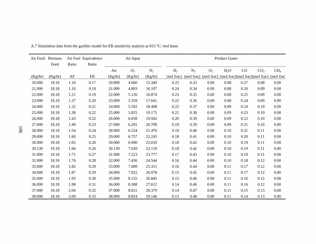
106
A.7 Simulation data from the gasifier model for ER sensitivity analysis at 815 °C: mol basis
Air Feed Biomass Air Fuel Equivalence Air Input Product Gases H
Feed Ratio Ratio Air O2 N2 2 N2 O2 H2O CO CO2 CH4
(Kg/hr) (Kg/hr) AF ER (Kg/hr) (Kg/hr) (Kg/hr) (mol frac) (mol frac) (mol frac) (mol frac)(mol frac)(mol frac) (mol frac)20.000 18.18 1.10 0.17 20.000 4.660 15.340 0.25 0.33 0.00 0.08 0.27 0.08 0.0021.000
18.18 1.16 0.18 21.000 4.893 16.107 0.24 0.34 0.00 0.08 0.26 0.09 0.0022.000 18.18 1.21 0.19 22.000 5.126 16.874 0.23 0.35 0.00 0.08 0.25 0.09 0.0023.000 18.18 1.27 0.20 23.000 5.359 17.641 0.22 0.36 0.00 0.08 0.24 0.09 0.0024.000 18.18 1.32 0.21 24.000 5.592 18.408 0.22 0.37 0.00 0.09 0.24 0.10 0.0025.000 18.18 1.38 0.22 25.000 5.825 19.175 0.21 0.38 0.00 0.09 0.23 0.10 0.0026.000 18.18 1.43 0.22 26.000 6.058 19.942 0.20 0.39 0.00 0.09 0.22 0.10 0.0027.000 18.18 1.49 0.23 27.000 6.291 20.709 0.19 0.39 0.00 0.09 0.21 0.10 0.0028.000 18.18 1.54 0.24 28.000 6.524 21.476 0.19 0.40 0.00 0.10 0.21 0.11 0.0029.000 18.18 1.60 0.25 29.000 6.757 22.243 0.18 0.41 0.00 0.10 0.20 0.11 0.0030.000 18.18 1.65 0.26 30.000 6.990 23.010 0.18 0.42 0.00 0.10 0.19 0.11 0.0030.130 18.18 1.66 0.26 30.130 7.020 23.110 0.18 0.42 0.00 0.10 0.19 0.11 0.0031.000 18.18 1.71 0.27 31.000 7.223 23.777 0.17 0.43 0.00 0.10 0.19 0.11 0.0032.000 18.18 1.76 0.28 32.000 7.456 24.544 0.16 0.44 0.00 0.10 0.18 0.12 0.0033.000 18.18 1.82 0.29 33.000 7.689 25.311 0.16 0.44 0.00 0.11 0.17 0.12 0.0034.000 18.18 1.87 0.29 34.000 7.922 26.078 0.15 0.45 0.00 0.11 0.17 0.12 0.0035.000 18.18 1.93 0.30 35.000 8.155 26.845 0.15 0.46 0.00 0.11 0.16 0.12 0.0036.000 18.18 1.98 0.31 36.000 8.388 27.612 0.14 0.46 0.00 0.11 0.16 0.12 0.0037.000 18.18 2.04 0.32 37.000 8.621 28.379 0.14 0.47 0.00 0.11 0.15 0.13 0.0038.000 18.18 2.09 0.33 38.000 8.854 29.146 0.13 0.48 0.00 0.11 0.14 0.13 0.00
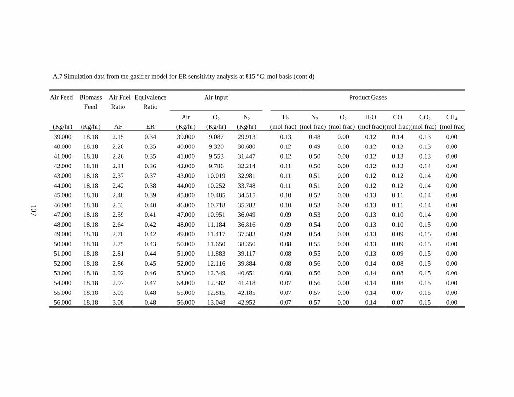
107
A.7 Simulation data from the gasifier model for ER sensitivity analysis at 815 °C: mol basis (cont’d)
Air Feed Biomass Air Fuel Equivalence Air Input Product Gases Feed Ratio Ratio H
Air O2 N2 2 N2 O2 H2O CO CO2 CH4
(Kg/hr) (Kg/hr) AF ER (Kg/hr) (Kg/hr) (Kg/hr) (mol frac) (mol frac) (mol frac) (mol frac)(mol frac)(mol frac) (mol frac)39.000 18.18 2.15 0.34 39.000 9.087 29.913 0.13 0.48 0.00 0.12 0.14 0.13 0.0040.000
18.18 2.20 0.35 40.000 9.320 30.680 0.12 0.49 0.00 0.12 0.13 0.13 0.0041.000 18.18 2.26 0.35 41.000 9.553 31.447 0.12 0.50 0.00 0.12 0.13 0.13 0.0042.000 18.18 2.31 0.36 42.000 9.786 32.214 0.11 0.50 0.00 0.12 0.12 0.14 0.0043.000 18.18 2.37 0.37 43.000 10.019 32.981 0.11 0.51 0.00 0.12 0.12 0.14 0.0044.000 18.18 2.42 0.38 44.000 10.252 33.748 0.11 0.51 0.00 0.12 0.12 0.14 0.0045.000 18.18 2.48 0.39 45.000 10.485 34.515 0.10 0.52 0.00 0.13 0.11 0.14 0.0046.000 18.18 2.53 0.40 46.000 10.718 35.282 0.10 0.53 0.00 0.13 0.11 0.14 0.0047.000 18.18 2.59 0.41 47.000 10.951 36.049 0.09 0.53 0.00 0.13 0.10 0.14 0.0048.000 18.18 2.64 0.42 48.000 11.184 36.816 0.09 0.54 0.00 0.13 0.10 0.15 0.0049.000 18.18 2.70 0.42 49.000 11.417 37.583 0.09 0.54 0.00 0.13 0.09 0.15 0.0050.000 18.18 2.75 0.43 50.000 11.650 38.350 0.08 0.55 0.00 0.13 0.09 0.15 0.0051.000 18.18 2.81 0.44 51.000 11.883 39.117 0.08 0.55 0.00 0.13 0.09 0.15 0.0052.000 18.18 2.86 0.45 52.000 12.116 39.884 0.08 0.56 0.00 0.14 0.08 0.15 0.0053.000 18.18 2.92 0.46 53.000 12.349 40.651 0.08 0.56 0.00 0.14 0.08 0.15 0.0054.000 18.18 2.97 0.47 54.000 12.582 41.418 0.07 0.56 0.00 0.14 0.08 0.15 0.0055.000 18.18 3.03 0.48 55.000 12.815 42.185 0.07 0.57 0.00 0.14 0.07 0.15 0.0056.000 18.18 3.08 0.48 56.000 13.048 42.952 0.07 0.57 0.00 0.14 0.07 0.15 0.00

108
A.7 Simulation data from the gasifier model for ER sensitivity analysis at 815 °C: mol basis (cont’d)
Air Feed Biomass Air Fuel Equivalence Air Input Product Gases Feed Ratio Ratio H
Air O2 N2 2 N2 O2 H2O CO CO2 CH4
(Kg/hr) (Kg/hr) AF ER (Kg/hr) (Kg/hr) (Kg/hr) (mol frac) (mol frac)(mol frac) (mol frac)(mol frac)(mol frac) (mol frac)57.000 18.18 3.14 0.49 57.000 13.281 43.719 0.06 0.57 0.00 0.14 0.07 0.16 0.00 58.000
18.18 3.19 0.50 58.000 13.514 44.486 0.06 0.58 0.00 0.14 0.06 0.16 0.0059.000 18.18 3.25 0.51 59.000 13.747 45.253 0.06 0.58 0.00 0.14 0.06 0.16 0.0060.000 18.18 3.30 0.52 60.000 13.980 46.020 0.05 0.59 0.00 0.14 0.06 0.16 0.0061.000 18.18 3.36 0.53 61.000 14.213 46.787 0.05 0.59 0.00 0.14 0.05 0.16 0.00

109
A.8 Simulation data from the gasifier model for ER sensitivity analysis at 750 °C: mol basis
Air Feed Biomass Air Fuel Equivalence Air Input Product Gases Feed Ratio Ratio H
Air O2 N2 2 N2 O2 H2O CO CO2 CH4
(Kg/hr) (Kg/hr) AF ER (Kg/hr) (Kg/hr) (Kg/hr) (mol frac) (mol frac) (mol frac) (mol frac)(mol frac)(mol frac) (mol frac)20.000 18.18 1.10 0.17 20.000 4.660 15.340 0.25 0.33 0.00 0.07 0.26 0.09 0.0021.000
18.18 1.16 0.18 21.000 4.893 16.107 0.24 0.34 0.00 0.07 0.25 0.10 0.0022.000 18.18 1.21 0.19 22.000 5.126 16.874 0.24 0.35 0.00 0.07 0.24 0.10 0.0023.000 18.18 1.27 0.20 23.000 5.359 17.641 0.23 0.36 0.00 0.08 0.23 0.10 0.0024.000 18.18 1.32 0.21 24.000 5.592 18.408 0.22 0.37 0.00 0.08 0.23 0.10 0.0025.000 18.18 1.38 0.22 25.000 5.825 19.175 0.22 0.38 0.00 0.08 0.22 0.11 0.0026.000 18.18 1.43 0.22 26.000 6.058 19.942 0.21 0.39 0.00 0.08 0.21 0.11 0.0027.000 18.18 1.49 0.23 27.000 6.291 20.709 0.20 0.40 0.00 0.09 0.20 0.11 0.0028.000 18.18 1.54 0.24 28.000 6.524 21.476 0.20 0.40 0.00 0.09 0.20 0.12 0.0029.000 18.18 1.60 0.25 29.000 6.757 22.243 0.19 0.41 0.00 0.09 0.19 0.12 0.0030.000 18.18 1.65 0.26 30.000 6.990 23.010 0.18 0.42 0.00 0.09 0.18 0.12 0.0030.130 18.18 1.66 0.26 30.130 7.020 23.110 0.18 0.42 0.00 0.09 0.18 0.12 0.0031.000 18.18 1.71 0.27 31.000 7.223 23.777 0.18 0.43 0.00 0.09 0.18 0.12 0.0032.000 18.18 1.76 0.28 32.000 7.456 24.544 0.17 0.44 0.00 0.10 0.17 0.12 0.0033.000 18.18 1.82 0.29 33.000 7.689 25.311 0.17 0.44 0.00 0.10 0.16 0.13 0.0034.000 18.18 1.87 0.29 34.000 7.922 26.078 0.16 0.45 0.00 0.10 0.16 0.13 0.0035.000 18.18 1.93 0.30 35.000 8.155 26.845 0.16 0.46 0.00 0.10 0.15 0.13 0.0036.000 18.18 1.98 0.31 36.000 8.388 27.612 0.15 0.46 0.00 0.10 0.15 0.13 0.0037.000 18.18 2.04 0.32 37.000 8.621 28.379 0.15 0.47 0.00 0.11 0.14 0.13 0.0038.000 18.18 2.09 0.33 38.000 8.854 29.146 0.14 0.48 0.00 0.11 0.14 0.14 0.00

110
A.8 Simulation data from the gasifier model for ER sensitivity analysis at 750 °C: mol basis (cont’d)
Air Feed Biomass Air Fuel Equivalence Air Input Product Gases Feed Ratio Ratio H
Air O2 N2 2 N2 O2 H2O CO CO2 CH4
(Kg/hr) (Kg/hr) AF ER (Kg/hr) (Kg/hr) (Kg/hr) (mol frac) (mol frac) (mol frac) (mol frac)(mol frac)(mol frac) (mol frac)39.000 18.18 2.15 0.34 39.000 9.087 29.913 0.14 0.48 0.00 0.11 0.13 0.14 0.0040.000
18.18 2.20 0.35 40.000 9.320 30.680 0.13 0.49 0.00 0.11 0.13 0.14 0.0041.000 18.18 2.26 0.35 41.000 9.553 31.447 0.13 0.50 0.00 0.11 0.12 0.14 0.0042.000 18.18 2.31 0.36 42.000 9.786 32.214 0.12 0.50 0.00 0.11 0.12 0.14 0.0043.000 18.18 2.37 0.37 43.000 10.019 32.981 0.12 0.51 0.00 0.12 0.11 0.14 0.0044.000 18.18 2.42 0.38 44.000 10.252 33.748 0.11 0.51 0.00 0.12 0.11 0.15 0.0045.000 18.18 2.48 0.39 45.000 10.485 34.515 0.11 0.52 0.00 0.12 0.10 0.15 0.0046.000 18.18 2.53 0.40 46.000 10.718 35.282 0.11 0.53 0.00 0.12 0.10 0.15 0.0047.000 18.18 2.59 0.41 47.000 10.951 36.049 0.10 0.53 0.00 0.12 0.10 0.15 0.0048.000 18.18 2.64 0.42 48.000 11.184 36.816 0.10 0.54 0.00 0.12 0.09 0.15 0.0049.000 18.18 2.70 0.42 49.000 11.417 37.583 0.09 0.54 0.00 0.13 0.09 0.15 0.0050.000 18.18 2.75 0.43 50.000 11.650 38.350 0.09 0.55 0.00 0.13 0.08 0.15 0.0051.000 18.18 2.81 0.44 51.000 11.883 39.884 0.09 0.55 0.00 0.13 0.08 0.16 0.0052.000 18.18 2.86 0.45 52.000 12.116 39.117 0.08 0.56 0.00 0.13 0.08 0.16 0.0053.000 18.18 2.92 0.46 53.000 12.349 40.651 0.08 0.56 0.00 0.13 0.07 0.16 0.0054.000 18.18 2.97 0.47 54.000 12.582 41.418 0.07 0.57 0.00 0.13 0.07 0.16 0.0055.000 18.18 3.03 0.48 55.000 12.815 42.185 0.07 0.57 0.00 0.13 0.06 0.16 0.0056.000 18.18 3.08 0.48 56.000 13.048 42.952 0.07 0.57 0.00 0.14 0.06 0.16 0.00

111
A.8 Simulation data from the gasifier model for ER sensitivity analysis at 750 °C: mol basis (cont’d)
Air Feed Biomass Air Fuel Equivalence Air Input Product Gases Feed Ratio Ratio H
Air O2 N2 2 N2 O2 H2O CO CO2 CH4
(Kg/hr) (Kg/hr) AF ER (Kg/hr) (Kg/hr) (Kg/hr) (mol frac) (mol frac) (mol frac)(mol frac)(mol frac)(mol frac) (mol frac)57.000 18.18 3.14 0.49 57.000 13.281 43.719 0.06 0.58 0.00 0.14 0.06 0.16 0.00 58.000
18.18 3.19 0.50 58.000 13.514 44.486 0.06 0.58 0.00 0.14 0.06 0.16 0.0059.000 18.18 3.25 0.51 59.000 13.747 45.253 0.06 0.59 0.00 0.14 0.05 0.16 0.0060.000 18.18 3.30 0.52 60.000 13.980 46.020 0.05 0.59 0.00 0.14 0.05 0.17 0.0061.000 18.18 3.36 0.53 61.000 14.213 46.787 0.05 0.60 0.00 0.14 0.05 0.17 0.00

112
A.9 Simulation data from the gasifier model for ER sensitivity analysis at 875 °C: mol basis
Air Feed Biomass Air Fuel Equivalence Air Input Product Gases H
Feed Ratio Ratio Air O2 N2 2 N2 O2 H2O CO CO2 CH4
(Kg/hr) (Kg/hr) AF ER (Kg/hr) (Kg/hr) (Kg/hr) (mol frac) (mol frac) (mol frac) (mol frac)(mol frac)(mol frac)(mol frac)20.000 18.18 1.10 0.17 20.000 4.660 15.340 0.24 0.33 0.00 0.08 0.27 0.08 0.0021.000
18.18 1.16 0.18 21.000 4.893 16.107 0.23 0.34 0.00 0.08 0.27 0.08 0.0022.000 18.18 1.21 0.19 22.000 5.126 16.874 0.22 0.35 0.00 0.09 0.26 0.08 0.0023.000 18.18 1.27 0.20 23.000 5.359 17.641 0.22 0.36 0.00 0.09 0.25 0.09 0.0024.000 18.18 1.32 0.21 24.000 5.592 18.408 0.21 0.37 0.00 0.09 0.24 0.09 0.0025.000 18.18 1.38 0.22 25.000 5.825 19.175 0.20 0.38 0.00 0.09 0.23 0.09 0.0026.000 18.18 1.43 0.22 26.000 6.058 19.942 0.20 0.39 0.00 0.10 0.23 0.10 0.0027.000 18.18 1.49 0.23 27.000 6.291 20.709 0.19 0.39 0.00 0.10 0.22 0.10 0.0028.000 18.18 1.54 0.24 28.000 6.524 21.476 0.18 0.40 0.00 0.10 0.21 0.10 0.0029.000 18.18 1.60 0.25 29.000 6.757 22.243 0.18 0.41 0.00 0.10 0.21 0.10 0.0030.000 18.18 1.65 0.26 30.000 6.990 23.010 0.17 0.42 0.00 0.11 0.20 0.11 0.0030.130 18.18 1.66 0.26 30.130 7.020 23.110 0.17 0.42 0.00 0.11 0.20 0.11 0.0031.000 18.18 1.71 0.27 31.000 7.223 23.777 0.16 0.43 0.00 0.11 0.19 0.11 0.0032.000 18.18 1.76 0.28 32.000 7.456 24.544 0.16 0.44 0.00 0.11 0.19 0.11 0.0033.000 18.18 1.82 0.29 33.000 7.689 25.311 0.15 0.44 0.00 0.11 0.18 0.11 0.0034.000 18.18 1.87 0.29 34.000 7.922 26.078 0.15 0.45 0.00 0.11 0.17 0.11 0.0035.000 18.18 1.93 0.30 35.000 8.155 26.845 0.14 0.46 0.00 0.12 0.17 0.12 0.0036.000 18.18 1.98 0.31 36.000 8.388 27.612 0.14 0.46 0.00 0.12 0.16 0.12 0.0037.000 18.18 2.04 0.32 37.000 8.621 28.379 0.13 0.47 0.00 0.12 0.16 0.12 0.0038.000 18.18 2.09 0.33 38.000 8.854 29.146 0.13 0.48 0.00 0.12 0.15 0.12 0.00
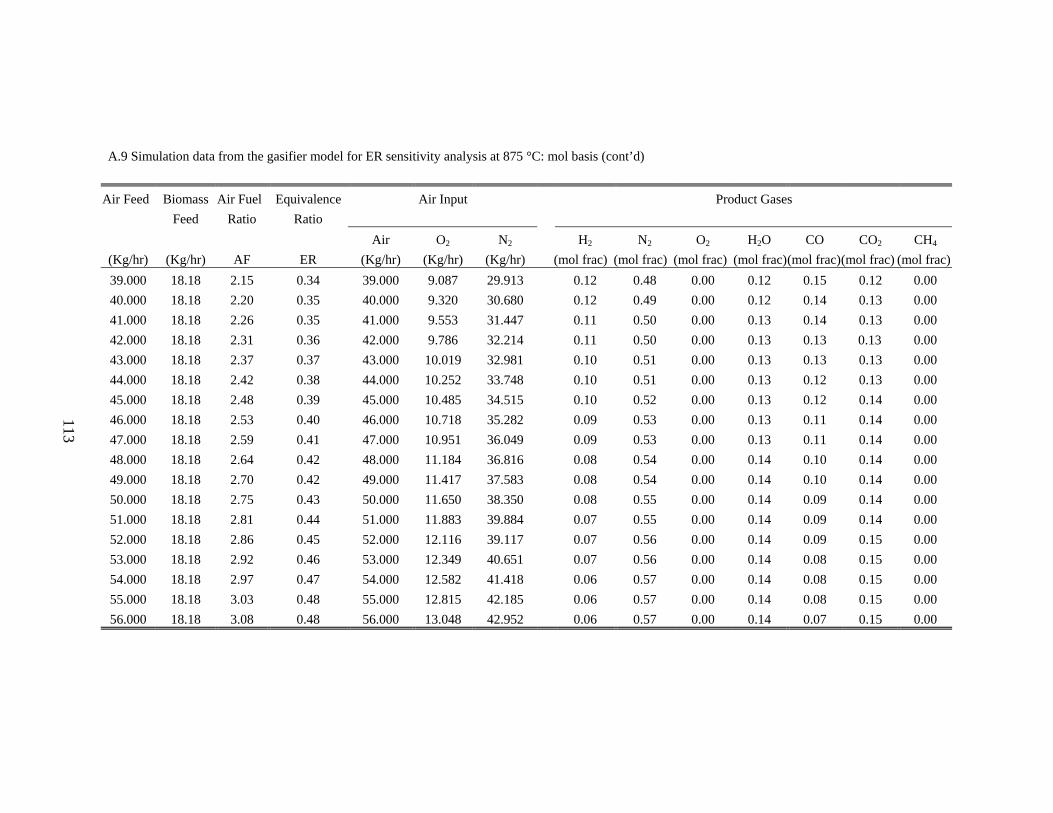
113
A.9 Simulation data from the gasifier model for ER sensitivity analysis at 875 °C: mol basis (cont’d)
Air Feed Biomass Air Fuel Equivalence Air Input Product Gases Feed Ratio Ratio H
Air O2 N2 2 N2 O2 H2O CO CO2 CH4
(Kg/hr) (Kg/hr) AF ER (Kg/hr) (Kg/hr) (Kg/hr) (mol frac) (mol frac) (mol frac) (mol frac)(mol frac)(mol frac) (mol frac)39.000 18.18 2.15 0.34 39.000 9.087 29.913 0.12 0.48 0.00 0.12 0.15 0.12 0.0040.000
18.18 2.20 0.35 40.000 9.320 30.680 0.12 0.49 0.00 0.12 0.14 0.13 0.0041.000 18.18 2.26 0.35 41.000 9.553 31.447 0.11 0.50 0.00 0.13 0.14 0.13 0.0042.000 18.18 2.31 0.36 42.000 9.786 32.214 0.11 0.50 0.00 0.13 0.13 0.13 0.0043.000 18.18 2.37 0.37 43.000 10.019 32.981 0.10 0.51 0.00 0.13 0.13 0.13 0.0044.000 18.18 2.42 0.38 44.000 10.252 33.748 0.10 0.51 0.00 0.13 0.12 0.13 0.0045.000 18.18 2.48 0.39 45.000 10.485 34.515 0.10 0.52 0.00 0.13 0.12 0.14 0.0046.000 18.18 2.53 0.40 46.000 10.718 35.282 0.09 0.53 0.00 0.13 0.11 0.14 0.0047.000 18.18 2.59 0.41 47.000 10.951 36.049 0.09 0.53 0.00 0.13 0.11 0.14 0.0048.000 18.18 2.64 0.42 48.000 11.184 36.816 0.08 0.54 0.00 0.14 0.10 0.14 0.0049.000 18.18 2.70 0.42 49.000 11.417 37.583 0.08 0.54 0.00 0.14 0.10 0.14 0.0050.000 18.18 2.75 0.43 50.000 11.650 38.350 0.08 0.55 0.00 0.14 0.09 0.14 0.0051.000 18.18 2.81 0.44 51.000 11.883 39.884 0.07 0.55 0.00 0.14 0.09 0.14 0.0052.000 18.18 2.86 0.45 52.000 12.116 39.117 0.07 0.56 0.00 0.14 0.09 0.15 0.0053.000 18.18 2.92 0.46 53.000 12.349 40.651 0.07 0.56 0.00 0.14 0.08 0.15 0.0054.000 18.18 2.97 0.47 54.000 12.582 41.418 0.06 0.57 0.00 0.14 0.08 0.15 0.0055.000 18.18 3.03 0.48 55.000 12.815 42.185 0.06 0.57 0.00 0.14 0.08 0.15 0.0056.000 18.18 3.08 0.48 56.000 13.048 42.952 0.06 0.57 0.00 0.14 0.07 0.15 0.00
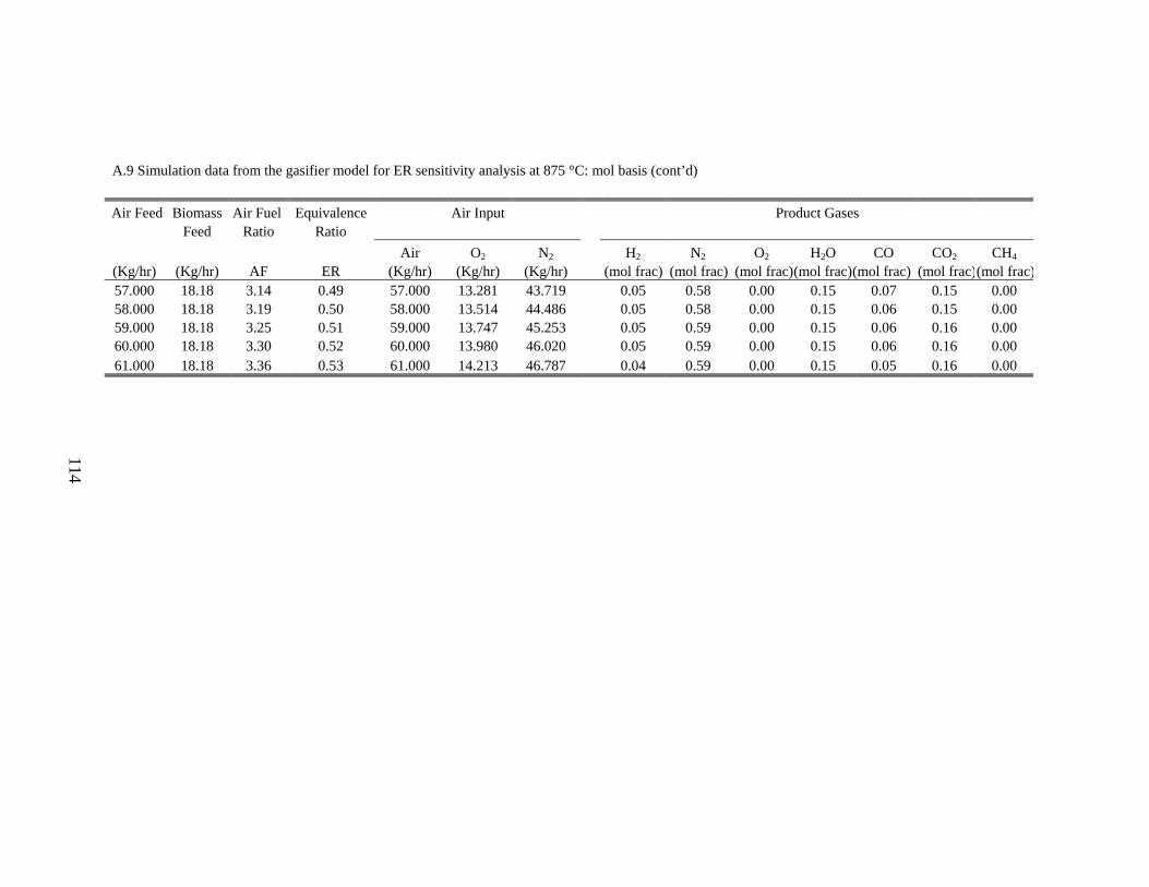
114
A.9 Simulation data from the gasifier model for ER sensitivity analysis at 875 °C: mol basis (cont’d)
Air Feed Biomass Air Fuel Equivalence Air Input Product Gases Feed Ratio Ratio H
Air O2 N2 2 N2 O2 H2O CO CO2 CH4
(Kg/hr) (Kg/hr) AF ER (Kg/hr) (Kg/hr) (Kg/hr) (mol frac) (mol frac) (mol frac)(mol frac)(mol frac) (mol frac)(mol frac)57.000 18.18 3.14 0.49 57.000 13.281 43.719 0.05 0.58 0.00 0.15 0.07 0.15 0.00 58.000
18.18 3.19 0.50 58.000 13.514 44.486 0.05 0.58 0.00 0.15 0.06 0.15 0.0059.000 18.18 3.25 0.51 59.000 13.747 45.253 0.05 0.59 0.00 0.15 0.06 0.16 0.0060.000 18.18 3.30 0.52 60.000 13.980 46.020 0.05 0.59 0.00 0.15 0.06 0.16 0.0061.000 18.18 3.36 0.53 61.000 14.213 46.787 0.04 0.59 0.00 0.15 0.05 0.16 0.00

115
A.10 Simulation data from the gasifier model for ER sensitivity analysis at 925 °C: mol basis
Air Feed Biomass Air Fuel Equivalence Air Input Product Gases H
Feed Ratio Ratio Air O2 N2 2 N2 O2 H2O CO CO2 CH4
(Kg/hr) (Kg/hr) AF ER (Kg/hr) (Kg/hr) (Kg/hr) (mol frac) (mol frac) (mol frac)(mol frac)(mol frac) (mol frac)(mol frac)20.000 18.18 1.10 0.17 20.000 4.660 15.340 0.24 0.33 0.00 0.09 0.28 0.07 0.0021.000
18.18 1.16 0.18 21.000 4.893 16.107 0.23 0.34 0.00 0.09 0.27 0.08 0.0022.000 18.18 1.21 0.19 22.000 5.126 16.874 0.22 0.35 0.00 0.09 0.26 0.08 0.0023.000 18.18 1.27 0.20 23.000 5.359 17.641 0.21 0.36 0.00 0.09 0.25 0.08 0.0024.000 18.18 1.32 0.21 24.000 5.592 18.408 0.20 0.37 0.00 0.10 0.25 0.09 0.0025.000 18.18 1.38 0.22 25.000 5.825 19.175 0.20 0.38 0.00 0.10 0.24 0.09 0.0026.000 18.18 1.43 0.22 26.000 6.058 19.942 0.19 0.39 0.00 0.10 0.23 0.09 0.0027.000 18.18 1.49 0.23 27.000 6.291 20.709 0.18 0.39 0.00 0.10 0.22 0.09 0.0028.000 18.18 1.54 0.24 28.000 6.524 21.476 0.18 0.40 0.00 0.11 0.22 0.10 0.0029.000 18.18 1.60 0.25 29.000 6.757 22.243 0.17 0.41 0.00 0.11 0.21 0.10 0.0030.000 18.18 1.65 0.26 30.000 6.990 23.010 0.16 0.42 0.00 0.11 0.20 0.10 0.0030.130 18.18 1.66 0.26 30.130 7.020 23.110 0.16 0.42 0.00 0.11 0.20 0.10 0.0031.000 18.18 1.71 0.27 31.000 7.223 23.777 0.16 0.43 0.00 0.11 0.20 0.10 0.0032.000 18.18 1.76 0.28 32.000 7.456 24.544 0.15 0.44 0.00 0.12 0.19 0.11 0.0033.000 18.18 1.82 0.29 33.000 7.689 25.311 0.15 0.44 0.00 0.12 0.18 0.11 0.0034.000 18.18 1.87 0.29 34.000 7.922 26.078 0.14 0.45 0.00 0.12 0.18 0.11 0.0035.000 18.18 1.93 0.30 35.000 8.155 26.845 0.14 0.46 0.00 0.12 0.17 0.11 0.0036.000 18.18 1.98 0.31 36.000 8.388 27.612 0.13 0.46 0.00 0.12 0.17 0.11 0.0037.000 18.18 2.04 0.32 37.000 8.621 28.379 0.13 0.47 0.00 0.12 0.16 0.12 0.0038.000 18.18 2.09 0.33 38.000 8.854 29.146 0.12 0.48 0.00 0.13 0.16 0.12 0.00

116
A.10 Simulation data from the gasifier model for ER sensitivity analysis at 925 °C: mol basis (cont’d)
Air Feed Biomass Air Fuel Equivalence Air Input Product Gases Feed Ratio Ratio H
Air O2 N2 2 N2 O2 H2O CO CO2 CH4
(Kg/hr) (Kg/hr) AF ER (Kg/hr) (Kg/hr) (Kg/hr) (mol frac) (mol frac) (mol frac) (mol frac)(mol frac)(mol frac)(mol frac)39.000 18.18 2.15 0.34 39.000 9.087 29.913 0.12 0.48 0.00 0.13 0.15 0.12 0.0040.000
0.13 0.07
51.000 0.07 52.000 0.07
54.000
18.18 2.20 0.35 40.000 9.320 30.680 0.11 0.49 0.00 0.13 0.15 0.12 0.0041.000 18.18 2.26 0.35 41.000 9.553 31.447 0.11 0.50 0.00 0.13 0.14 0.12 0.0042.000 18.18 2.31 0.36 42.000 9.786 32.214 0.10 0.50 0.00 0.13 0.14 0.13 0.0043.000 18.18 2.37 0.37 43.000 10.019 32.981 0.10 0.51 0.00 0.13 0.13 0.13 0.0044.000 18.18 2.42 0.38 44.000 10.252 33.748 0.10 0.51 0.00 0.13 0.13 0.13 0.0045.000 18.18 2.48 0.39 45.000 10.485 34.515 0.09 0.52 0.00 0.14 0.12 0.13 0.0046.000 18.18 2.53 0.40 46.000 10.718 35.282 0.09 0.53 0.00 0.14 0.12 0.0047.000 18.18 2.59 0.41 47.000 10.951 36.049 0.08 0.53 0.00 0.14 0.11 0.13 0.0048.000 18.18 2.64 0.42 48.000 11.184 36.816 0.08 0.54 0.00 0.14 0.11 0.14 0.0049.000 18.18 2.70 0.42 49.000 11.417 37.583 0.08 0.54 0.00 0.14 0.10 0.14 0.0050.000 18.18 2.75 0.43 50.000 11.650 38.350 0.55 0.00 0.14 0.10 0.14 0.00
18.18 2.81 0.44 51.000 11.883 39.884 0.55 0.00 0.14 0.09 0.14 0.0018.18 2.86 0.45 52.000 12.116 39.117 0.56 0.00 0.14 0.09 0.14 0.00
53.000 18.18 2.92 0.46 53.000 12.349 40.651 0.06 0.56 0.00 0.15 0.09 0.14 0.0018.18 2.97 0.47 54.000 12.582 41.418 0.06 0.57 0.00 0.15 0.08 0.15 0.00
55.000 18.18 3.03 0.48 55.000 12.815 42.185 0.06 0.57 0.00 0.15 0.08 0.15 0.0056.000 18.18 3.08 0.48 56.000 13.048 42.952 0.05 0.57 0.00 0.15 0.07 0.15 0.00

A.10 Simulation data from the gasifier model for ER sensitivity analysis at 925 °C: mol basis (cont’d)
Air Feed Biomass Air Fuel Equivalence Air Input Product Gases Feed Ratio Ratio Air O2 N2 H2 N2 O2 H2O CO CO2 CH4
(Kg/hr) (Kg/hr) AF ER (Kg/hr) (Kg/hr) (Kg/hr) (mol frac) (mol frac) (mol frac) (mol frac)(mol frac)(mol frac) (mol frac)57.000 18.18 3.14 0.49 57.000 13.281 43.719 0.05 0.58 0.00 0.15 0.07 0.15 0.00 58.000
18.18 3.19 0.50 58.000 13.514 44.486 0.05 0.58 0.00 0.15 0.07 0.15 0.0059.000 18.18 3.25 0.51 59.000 13.747 45.253 0.05 0.59 0.00 0.15 0.06 0.15 0.0060.000 18.18 3.30 0.52 60.000 13.980 46.020 0.04 0.59 0.00 0.15 0.06 0.15 0.0061.000 18.18 3.36 0.53 61.000 14.213 46.787 0.04 0.59 0.00 0.15 0.06 0.16 0.00
117
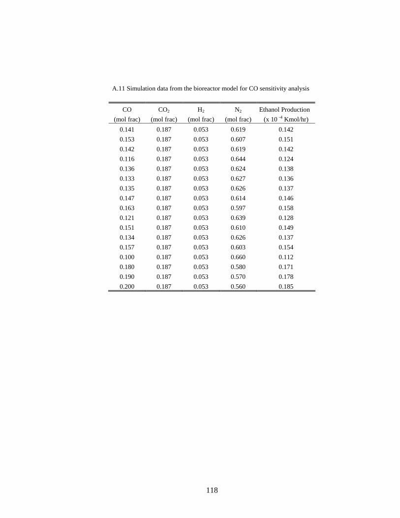
A.11 Simulation data from the bioreactor model for CO sensitivity analysis
CO CO2 H2 N2 Ethanol Production (mol frac) (mol frac) (mol frac) (mol frac) (x 10 -4 Kmol/hr)
0.141 0.187 0.053 0.619 0.142 0.153 0.187 0.053 0.607 0.151 0.142 0.187 0.053 0.619 0.142 0.116 0.187 0.053 0.644 0.124 0.136 0.187 0.053 0.624 0.138 0.133 0.187 0.053 0.627 0.136 0.135 0.187 0.053 0.626 0.137 0.147 0.187 0.053 0.614 0.146 0.163 0.187 0.053 0.597 0.158 0.121 0.187 0.053 0.639 0.128 0.151 0.187 0.053 0.610 0.149 0.134 0.187 0.053 0.626 0.137 0.157 0.187 0.053 0.603 0.154 0.100 0.187 0.053 0.660 0.112 0.180 0.187 0.053 0.580 0.171 0.190 0.187 0.053 0.570 0.178 0.200 0.187 0.053 0.560 0.185
118

A.12 Simulation data from the bioreactor model for CO2 sensitivity analysis
CO CO2 H2 N2
Ethanol Production (mol frac) (mol frac) (mol frac) (mol frac) (x 10 -4 Kmol/hr)
0.141 0.184 0.053 0.623 0.14171 0.141 0.182 0.053 0.625 0.14171 0.141 0.179 0.053 0.627 0.14171 0.141 0.177 0.053 0.629 0.14171 0.141 0.182 0.053 0.625 0.14171 0.141 0.183 0.053 0.623 0.14171 0.141 0.186 0.053 0.621 0.14171 0.141 0.192 0.053 0.614 0.14172 0.141 0.192 0.053 0.615 0.14172 0.141 0.205 0.053 0.601 0.14174 0.141 0.186 0.053 0.621 0.14171 0.141 0.193 0.053 0.613 0.14172 0.141 0.186 0.053 0.621 0.14171 0.141 0.150 0.053 0.657 0.14167 0.141 0.160 0.053 0.647 0.14168 0.141 0.210 0.053 0.597 0.14170 0.141 0.110 0.053 0.697 0.14170 0.141 0.250 0.053 0.557 0.14170
119

A.13 Simulation data from the bioreactor model for H2 sensitivity analysis
CO CO2 H2 N2
Ethanol Production (mol frac) (mol frac) (mol frac) (mol frac) (x 10 -4 Kmol/hr)
0.14 0.19 0.09 0.58 0.169 0.14 0.19 0.06 0.61 0.146 0.14 0.19 0.06 0.61 0.147 0.14 0.19 0.05 0.62 0.141 0.14 0.19 0.04 0.63 0.131 0.14 0.19 0.05 0.62 0.139 0.14 0.19 0.05 0.62 0.141 0.14 0.19 0.05 0.62
0.19
0.19 0.60
0.138 0.14 0.19 0.06 0.62 0.144 0.14 0.19 0.06 0.61 0.149 0.14 0.05 0.63 0.137 0.14 0.19 0.06 0.61 0.145 0.14 0.19 0.05 0.62 0.139 0.14 0.19 0.06 0.61 0.148 0.14 0.03 0.64 0.125 0.14 0.19 0.07 0.155
120
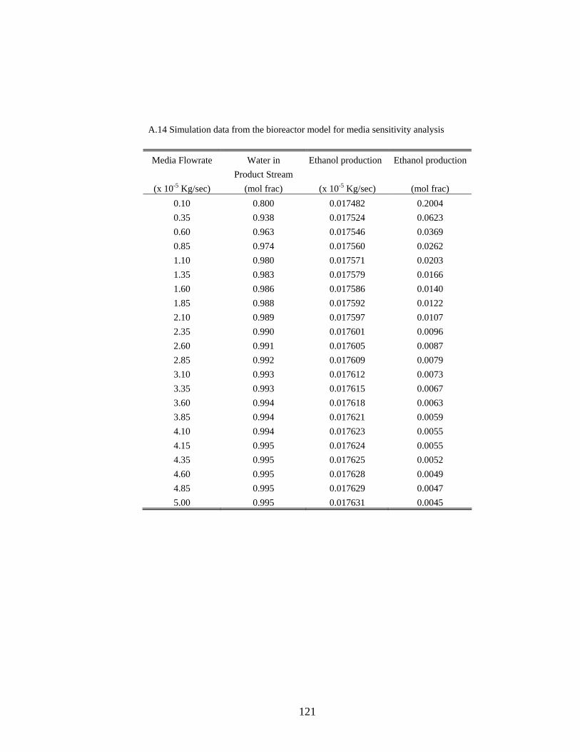
121
A.14 Simulation data from the bioreactor model for media sensitivity analysis
Media Flowrate Water in Ethanol production Ethanol production Product Stream
(x 10-5 Kg/sec) (mol frac) (x 10-5 Kg/sec) (mol frac) 0.10 0.800 0.017482 0.2004 0.35 0.938 0.017524 0.0623 0.60 0.963 0.017546 0.0369 0.85 0.974 0.017560 0.0262 1.10 0.980 0.017571 0.0203 1.35 0.983 0.017579 0.0166 1.60 0.986 0.017586 0.0140 1.85 0.988 0.017592 0.0122 2.10 0.989 0.017597 0.0107 2.35 0.990 0.017601 0.0096 2.60 0.991 0.017605 0.0087 2.85 0.992 0.017609 0.0079 3.10 0.993 0.017612 0.0073 3.35 0.993 0.017615 0.0067 3.60 0.994 0.017618 0.0063 3.85 0.994 0.017621 0.0059 4.10 0.994 0.0055 4.15 0.995 0.017624 0.0055 4.35 0.995 0.017625 0.0052 4.60 0.995
0.017623
0.017628 0.0049 4.85 0.995 0.017629 0.0047 5.00 0.995 0.017631 0.0045
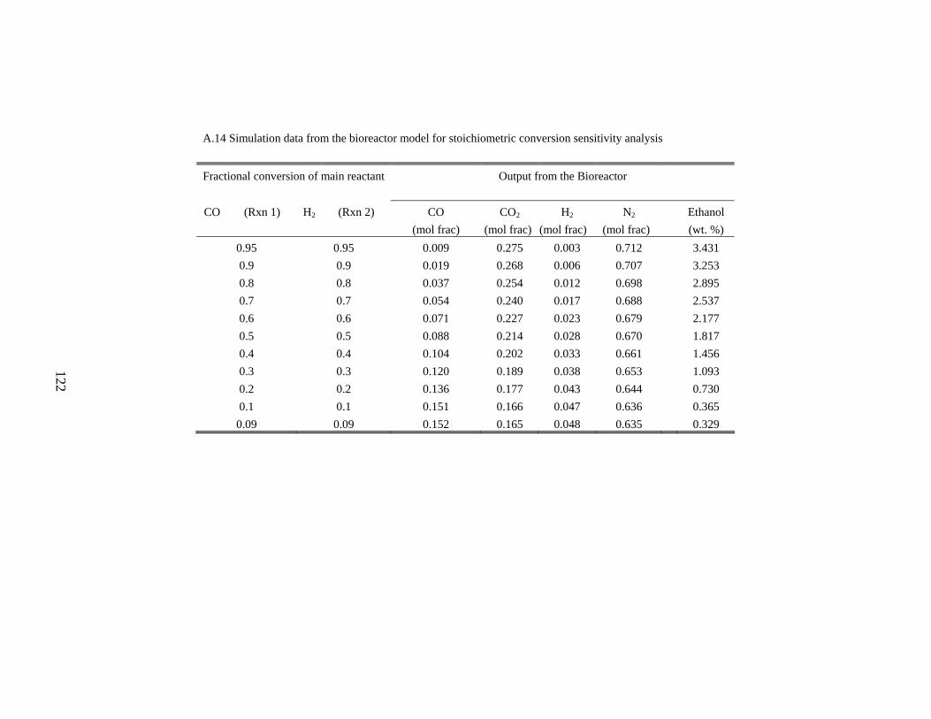
122
A.14 Simulation data from the bioreactor model for stoichiometric conversion sensitivity analysis
Fractional conversion of main reactant Output from the Bioreactor
(Rxn 1) H2 CO CO2 H2 N2
CO (Rxn 2) Ethanol (mol frac) (mol frac) (mol frac) (mol frac) (wt. %)
0.95 0.95 0.009 0.275 0.003 0.712 3.4310.9
0.9 0.019 0.268 0.006 0.707 3.2530.8 0.8 0.037 0.254 0.012 0.698 2.8950.7 0.7 0.054 0.240 0.017 0.688 2.5370.6 0.6 0.071 0.227 0.023 0.679 2.1770.5 0.5 0.088 0.214 0.028 0.670 1.8170.4 0.4 0.104 0.202 0.033 0.661 1.4560.3 0.3 0.120 0.189 0.038 0.653 1.0930.2 0.2 0.136 0.177 0.043 0.644 0.7300.1 0.1 0.151 0.166 0.047 0.636 0.365
0.09 0.09 0.152 0.165 0.048 0.635 0.329

123
A.15 Simulation data from the bioreactor model for stoichiometric conversion (E1) sensitivity analysis
Fractional conversion of main reactant Output from the Bioreactor
(Rxn 1) H2 CO CO2 H2 N2
CO (Rxn 2) Ethanol
(mol frac) (mol frac) (mol frac) (mol frac) (wt. %) 0.9 0.1 0.017 0.266 0.048 0.669 2.5460.8
0.1 0.034 0.253 0.048 0.665 2.2730.7 0.1 0.051 0.240 0.048 0.661 1.9990.6 0.1 0.068 0.227 0.047 0.657 1.7260.5 0.1 0.085 0.215 0.047 0.653 1.4520.4 0.1 0.101 0.202 0.047 0.650 1.1790.3 0.1 0.117 0.190 0.047 0.646 0.9050.2 0.1 0.133 0.178 0.046 0.643 0.6320.1 0.1 0.149 0.166 0.046 0.639 0.358

A.16 Simulation data from the bioreactor model for stoichiometric conversion (E2) sensitivity analysis
Fractional conversion of main reactant Output from the Bioreactor
(Rxn 1) H2 CO CO2 H2 N2
CO (Rxn 2) Ethanol
(mol frac) (mol frac) (mol frac) (mol frac) (wt. %) 0.1 0.9 0.157 0.161 0.005 0.676 1.0340.1
0.1 0.6 0.154 0.02
0.026 0.65 0.4 0.152 0.164 0.031 0.652 0.612
0.1 0.1
0.04
0.8 0.156 0.162 0.011 0.671 0.9500.1 0.7 0.155 0.162 0.016 0.666 0.865
0.163 1 0.662 0.7810.1 0.5 0.153 0.164 7 0.6960.1
0.3 0.151 0.165 0.036 0.648 0.5270.2 0.150 0.165 0.041 0.643 0.443
0.1 0.1 0.149 0.166 6 0.639 0.358
124

APPENDIX B
ASPEN PLUS™ INPUT AND OUTPUT FILES
125

The simulation output data in Aspen PlusTM is displayed in an output table form on the process flowsheet. The input and the output from the Base Case simulation for the Gibbs gasifier model is shown in Appendix B.1 and the input and the output from the Base Case simulation for the stoichiometric bioreactor model is shown in Appendix B.2.
126

B1. Simulation output data table from the Gibbs Gasifier model
Gsfr-RGIBBS-12
Stream ID AIR BIOMASS PRODUCT
From RGIBBS
To RGIBBS RGIBBS
Phase VAPOR MIXED VAPOR
Substream: MIXED
Mole Flow kmol/hr
C 0.0 .5977854 4.0015E-28
H2 0.0 .4514158 .3455666
O2 .2193832 .2428216 6.0119E-19
N2 .8249600 4.99759E-3 .8299576 H2O 0.0 .0910338 .1967083
CO 0.0 0.0 .3766608
CO2 0.0 0.0 .2210372
CH4 0.0 0.0 8.73577E-5
NO 0.0 0.0 1.4735E-13
NO2 0.0 0.0 5.2839E-24
C2H2 0.0 0.0 4.5733E-12
C2H4 0.0 0.0 6.9141E-11
C2H6 0.0 0.0 8.1647E-12
Mole Frac
C 0.0 .4306643 2.0312E-28
H2 0.0 .3252148 .1754129
O2 .2100681 .1749367 3.0517E-19
N2 .7899319 3.60043E-3 .4212945
H2O 0.0 .0655837 .0998510
CO 0.0 0.0 .1911966
CO2 0.0 0.0 .1122006
CH4 0.0 0.0 4.43436E-5
NO 0.0 0.0 7.4798E-14
NO2 0.0 0.0 2.6822E-24
C2H2 0.0 0.0 2.3214E-12
C2H4 0.0 0.0 3.5096E-11
C2H6 0.0 0.0 4.1445E-12Mass Flow kg/hr
C 0.0 7.180000 4.8061E-27
H2 0.0 .9100000 .6966208
O2 7.020000 7.770000 1.9237E-17
N2 23.11000 .1400000 23.25000
H2O 0.0 1.640000 3.543755
CO 0.0 0.0 10.55042
CO2 0.0 0.0 9.727804
CH4 0.0 0.0 1.40146E-3
NO 0.0 0.0 4.4215E-12
NO2 0.0 0.0 2.4309E-22
C2H2 0.0 0.0 1.1908E-10
C2H4 0.0 0.0 1.93965E-9
C2H6 0.0 0.0 2.4551E-10
Mass Frac
C 0.0 .4070295 1.0061E-28
H2 0.0 .0515873 .0145828
O2 .2329904 .4404762 4.0271E-19
N2 .7670096 7.93651E-3 .4867071
H2O 0.0 .0929705 .0741836
CO 0.0 0.0 .2208587
CO2 0.0 0.0 .2036383 CH4 0.0 0.0 2.93376E-5
NO 0.0 0.0 9.2559E-14
NO2 0.0 0.0 5.0887E-24
C2H2 0.0 0.0 2.4927E-12
C2H4 0.0 0.0 4.0604E-11
C2H6 0.0 0.0 5.1394E-12
Total Flow kmol/hr 1.044343 1.388054 1.970018
Total Flow kg/hr 30.13000 17.64000 47.77000
Total Flow l/min 354.8593 249.7050 2931.692
Temperature K 298.1500 298.1500 1088.150
Pressure atm 1.200000 1.200000 1.000000
Vap or Frac 1.000000 .5051573 1.000000
Liquid Frac 0.0 .4948427 0.0
Solid Frac 0.0 0.0 0.0
Enthalpy cal/mol 7.0286E-13 60663.34 -15074.27
Enthalpy cal/gm 2.4362E-14 4773.469 -621.6574
Enthalpy cal/sec 2.0390E-13 23390.00 -8249.049
Entropy cal/mol-K .6587547 113.9860 16.11036
Entropy cal/gm-K .0228332 8.969319 .6643853
Density mol/cc 4.90496E-5 9.26463E-5 1.11996E-5
Density gm/cc 1.41512E-3 1.17739E-3 2.71572E-4
Average MW 28.85067 12.70844 24.24851
Liq Vol 60F l/min .9322121 .7258234 1.642086
127

B.2 Simulation output data table from the stoichiometric bioreactor model
BR-Rstoic-7
Stream ID GASES MEDIA PRODGAS PRODMED PRODUCT
From SEP2 SEP2 RST OIC
To RST OIC RST OIC SEP2
Phase VAPOR LIQUID VAPOR LIQUID MIXED
Subst ream: MIXED
Mole Flow kmol/sec
ET HANOL 0.0 0.0 0.0 4.7371E-10 4.7371E-10
WATER 0.0 3.30891E-7 0.0 3.30151E-7 3.30151E-7
H2 6.81463E-9 0.0 6.13317E-9 0.0 6.13317E-9
N2 8.21680E-8 0.0 8.21680E-8 0.0 8.21680E-8
CO 2.16080E-8 0.0 1.94472E-8 0.0 1.94472E-8
CO2 2.02085E-8 0.0 2.14218E-8 0.0 2.14218E-8
Mole Frac
ET HANOL 0.0 0.0 0.0 1.43277E-3 1.03027E-3
WATER 0.0 1.000000 0.0 .9985672 .7180397
H2 .0521000 0.0 .0474813 0.0 .0133389
N2 .6282000 0.0 .6361218 0.0 .1787057
CO .1652000 0.0 .1505549 0.0 .0422953
CO2 .1545000 0.0 .1658420 0.0 .0465899
Mass Flow kg/sec
ET HANOL 0.0 0.0 0.0 2.18234E-8 2.18234E-8
WATER 0.0 5.96109E-6 0.0 5.94776E-6 5.94776E-6
H2 1.37375E-8 0.0 1.23637E-8 0.0 1.23637E-8
N2 2.30181E-6 0.0 2.30181E-6 0.0 2.30181E-6
CO 6.05249E-7 0.0 5.44724E-7 0.0 5.44724E-7
CO2 8.89370E-7 0.0 9.42770E-7 0.0 9.42770E-7
Mass Frac
ET HANOL 0.0 0.0 0.0 3.65576E-3 2.23343E-3
WATER 0.0 1.000000 0.0 .9963442 .6087000
H2 3.60548E-3 0.0 3.25219E-3 0.0 1.26532E-3
N2 .6041233 0.0 .6054737 0.0 .2355696
CO .1588510 0.0 .1432855 0.0 .0557475
CO2 .2334202 0.0 .2479886 0.0 .0964840
Total Flow kmol/sec 1.30799E-7 3.30891E-7 1.29170E-7 3.30625E-7 4.59795E-7
Total Flow kg/sec 3.81017E-6 5.96109E-6 3.80167E-6 5.96959E-6 9.77125E-6
Total Flow cum/sec 2.66667E-6 6.00000E-9 3.28734E-6 6.08510E-9 3.49050E-6
Temperature K 298.1500 298.1500 310.1500 310.1500 310.1500
Pressure N/sqm 1.21590E+5 1.21590E+5 1.01325E+5 1.01325E+5 1.01325E+5
Vapor Frac 1.000000 0.0 1.000000 0.0 .2977827
Liquid Frac 0.0 1.000000 0.0 1.000000 .7022173
Solid Frac 0.0 0.0 0.0 0.0 0.0
Enthalpy J/kmol -7.9057E+7 -2.8568E+8 -8.1535E+7 -2.8483E+8 -2.2691E+8
Enthalpy J/kg -2.7139E+6 -1.5858E+7 -2.7703E+6 -1.5775E+7 -1.0677E+7
Enthalpy Wat t -10.34056 -94.52996 -10.53191 -94.17258 -104 .3322
Entropy J/kmol-K 22259 .69 -1.6269E+5 23567 .62 -1.6014E+5 -1.0576E+5
Entropy J/kg-K 764.1518 -9030.528 800.7625 -8869.457 -4976.398
Density kmol/cum .0490496 55.14843 .0392932 54.33350 .1317276
Density kg/cum 1.428812 993.5145 1.156457 981.0171 2.799387
Average MW 29.12993 18.01528 29.43148 18.05547 21.25134
Liq Vol 60F cum/sec 7.00531E-9 5.97258E-9 6.91807E-9 5.98678E-9 1.29049E-8
128

VITA
Sirigudi Rahul Rao
Candidate for the Degree of
Master of Science
Thesis: BIOMASS TO ETHANOL: PROCESS SIMULATION, VALIDATION AND SENSITIVITY ANALYSIS OF A GASIFIER AND A BIOREACTOR
Major Field: Chemical Engineering Biographical Information:
Personal Data: Born in Mumbai, India, on the 24th of September, 1979, the son of Sirigudi Ramakrishna Rao and Sirigudi Vijayalakshmi Rao.
Education: Graduated from Holy Cross Higher Secondary School, Byron Bazar,
Raipur, India in May 1997; received Bachelor of Engineering degree in Chemical Engineering from National Institute of Technology, Karnataka, India, in June 2002. Completed the requirements for the Master of Science degree in Chemical Engineering at Oklahoma State University, Stillwater, Oklahoma, in December, 2005.
Experience: Summer Internship at Bhilai Steel Plant, India, 2000; employed as a
Graduate Engineer Trainee at Bharat Aluminum Company, Korba, India, June 2002 to May 2003; employed by Oklahoma State University, Department of Chemical Engineering as a Research Assistant, August 2003 to August 2005; Teaching Assistant, August 2003 to December 2003, August 2004 to December 2004 and January 2005 to May 2005.

Name: Sirigudi Rahul Rao Date of Degree: December, 2005 Institution: Oklahoma State University Location: Stillwater, Oklahoma Title of Study: BIOMASS TO ETHANOL: PROCESS SIMULATION, VALIDATION
AND SENSITIVITY ANALYSIS OF A GASIFIER AND A BIOREACTOR
Pages in Study: 128 Candidate for the Degree of Master of Science
Major Field: Chemical Engineering Scope and Method of Study: The Gasification-Fermentation process for the production of
fuel-grade ethanol from agricultural biomass is being investigated at Oklahoma State University, Stillwater. Process simulation software, Aspen Plus™ was used to study the gasifier and the bioreactor set-ups in this research. Process models were developed and validated with experimental data. Sensitivity studies were conducted for the gasifier by manipulating important process parameters like biomass feed rate, moisture content, operating temperature and equivalence ratio. Sensitivity of the bioreactor model was studied by manipulating the input gas composition of carbon monoxide, carbon dioxide and hydrogen gases, media flow rate, and stoichiometric conversion of substrates.
Findings and Conclusions: The results from this work indicate that, the amount of carbon
monoxide and hydrogen gases produced in the gasifier and the amount of ethanol produced in the bioreactor can theoretically be improved further.
ADVISER’S APPROVAL: Arland H. Johannes
Top Related