


Languages
Pages
Legal


21
3.5. GIS Data Models:
3.5.1. Spatial Data Models
Traditionally spatial data has been stored and presented in the form of a map. Three basic types of
spatial data models have evolved for storing geographic data digitally. These are referred to as :
• Vector
• Raster
• Image
The following diagram reflects the two primary spatial data encoding techniques. These are vector and
raster. Image data utilizes techniques very similar to raster data, however typically lacks the
internal formats required for analysis and modeling of the data. Images reflects pictures or photographs
of the landscape.
3.5.2. Vector Data Formats
All spatial data models are approaches for storing the spatial location of geographic features in a
database. Vector storage implies the use of vectors (directional lines) to represent a geographic feature.
Vector data is characterized by the use of sequential points or vertices to define a linear segment. Each
vertex consists of an X coordinate and a Y coordinate.
Vector lines are often referred to as arcs and consist of a string of vertices terminated by a node. A
node is defined as a vertex that starts or ends an arc segment. Point features are defined by one
coordinate pair, a vertex. Polygonal features are defined by a set of closed coordinate pairs. In vector
representation, the storage of the vertices for each feature is important, as well as the connectivity
between features, e.g. the sharing of common vertices where features connect.
Point representations

22
Points are defined as single coordinate pairs (x, y) when we work in 2D or coordinate triplets (x, y, z)
when we work in 3D. Points are used to represent objects that are best described as shape- and sizeless,
single-locality features. Whether this is the case really depends on the purposes of the spatial
application and also on the spatial extent of the objects compared to the scale applied in the
application. For a tourist city map, parks will not usually be considered as point features, but perhaps
museums will be, and certainly public phone booths could be represented as point features.
Besides the georeference, usually extra data is stored for each point object. This so-called administrative
or thematic data, can capture anything that is considered relevant about the object. For phone booth
objects, this may include the owning telephone company, the phone number, the data last serviced et
cetera.
Line representations
Line data are used to represent one-dimensional objects such as roads, railroads, canals, rivers and
power lines. Again, there is an issue of relevance for the application and the scale that the application
requires. For the example application of mapping tourist information, bus, subway and streetcar routes
are likely to be relevant line features. Some cadastral systems, on the other hand, may consider roads to
be two-dimensional features, i.e., having a width as well.
The two end nodes and zero or more internal nodes define a line. Another word for internal node is
vertex (plural: vertices); another phrase for line that is used in some GISs is polyline, arc or edge. A node
or vertex is like a point (as discussed above) but it only serves to define the line; it has no special
meaning to the application other than that.
The vertices of a line help to shape it, and to obtain a better approximation of the actual feature. The
straight parts of a line between two consecutive vertices or end nodes are called line segments. Many
GISs store a line as a simple sequence of coordinates of its end nodes and vertices, assuming that all its
segments are straight. This is usually good enough, as cases in which a single straight line segment is
considered an unsatisfactory representation can be dealt with by using multiple (smaller) line segments
instead of only one.
Still, there are cases in which we would like to have the opportunity to use arbitrary curvilinear features
as representation of real-world phenomena. Think of garden design with perfect circular or elliptical
lawns, or of detailed topographic maps representing roundabouts and the annex sidewalks. All of this
can be had in GIS in principle, but many systems do not at present accommodate such shapes. If a GIS
supports some of these curvilinear features, it does so using parameterized mathematical descriptions.

23
Collections of (connected) lines may represent phenomena that are best viewed as networks. With
networks, specific type of interesting questions arise, that have to do with connectivity and network
capacity. Such issues come up in traffic monitoring, watershed management and other application
domains. With network elements—i.e., the lines that make up the network—extra values are commonly
associated like distance, quality of the link, or carrying capacity.
Area representations
When area objects are stored using a vector approach, the usual technique is to apply a boundary
model. This means that each area feature is represented by some arc/node structure that determines a
polygon as the area's boundary. Common sense dictates that area features of the same kind are best
stored in a single data layer, represented by mutually non-overlapping polygons. In essence, what we
then get is an application-determined (i.e., adaptive) partition of space, similar to, but not quite like an
irregular tessellation of the raster approach.
Observe that a polygon representation for an area object is yet another example of a finite
approximation of a phenomenon that inherently may have a curvilinear boundary. In the case that the
object can be perceived as having a fuzzy boundary, a polygon is an even worse approximation, though
potentially the only one possible.
A simple but naive representation of area features would be to list for each polygon simply the list of
lines that describes its boundary. Each line in the list would, as before, be a sequence that starts with a
node and ends with one, possibly with vertices in between. But this is far from optimal.
3.5.3. Raster Data Formats
Raster data models incorporate the use of a grid-cell data structure where the geographic area is
divided into cells identified by row and column. This data structure is commonly called raster. While the

24
term raster implies a regularly spaced grid other tessellated data structures do exist in grid based
GIS systems.
The size of cells in a tessellated data structure is selected on the basis of the data accuracy and the
resolution needed by the user. There is no explicit coding of geographic coordinates required since
that is implicit in the layout of the cells. A raster data structure is in fact a matrix where any coordinate
can be quickly calculated if the origin point is known, and the size of the grid cells is known. Since grid-
cells can be handled as two-dimensional arrays in computer encoding many analytical operations are
easy to program. This makes tessellated data structures a popular choice for many GIS software.
Topology is not a relevant concept with tessellated structures since adjacency and connectivity are
implicit in the location of a particular cell in the data matrix.
Most raster based GIS software requires that the raster cell contain only a single discrete value.
Accordingly, a data layer, e.g. forest inventory stands, may be broken down into a series of raster maps,
each representing an attribute type, e.g. a species map, a height map, a density map, etc. These are
often referred to as one attribute maps. This is in contrast to most conventional vector data models that
maintain data as multiple attribute maps, e.g. forest inventory polygons linked to a database table
containing all attributes as columns. This basic distinction of raster data storage provides the
foundation for quantitative analysis techniques. This is often referred to as raster or map algebra. The
use of raster data structures allow for sophisticated mathematical modelling processes while vector
based systems are often constrained by the capabilities and language of a relational DBMS.
Real world road Vector Representation as Line Raster Representation
3.5.4. Attribute Data Models
A separate data model is used to store and maintain attribute data for GIS software. These data
models may exist internally within the GIS software, or may be reflected in external commercial

25
Database Management Software (DBMS). A variety of different data models exist for the storage and
management of attribute data. The Relational Model is the most commonly used data model.
The relational database organizes data in tables. Each table, is identified by a unique table name, and is
organized by rows and columns. Each column within a table also has a unique name. Columns store the
values for a specific attribute, e.g. cover group, tree height. Rows represent one record in the table. In a
GIS each row is usually linked to a separate spatial feature, e.g. a forestry stand. Accordingly, each
row would be comprised of several columns, each column containing a specific value for that
geographic feature. The following figure presents a sample table for forest inventory features. This table
has 4 rows and 5 columns. The forest stand number would be the label for the spatial feature as well as
the primary key for the database table. This serves as the linkage between the spatial definition of the
feature and the attribute data for the feature.
Data is often stored in several tables. Tables can be joined or referenced to each other by common
columns (relational fields). Usually the common column is an identification number for a selected
geographic feature, e.g. a forestry stand polygon number. This identification number acts as the
primary key for the table. The ability to join tables through use of a common column is the essence of
the relational model. Such relational joins are usually ad hoc in nature and form the basis of for querying
in a relational GIS product. Unlike the other previously discussed database types, relationships are
implicit in the character of the data as opposed to explicit characteristics of the database set up.
3.6. General spatial topology
Topology deals with spatial properties that do not change under certain transformations. These
relationships are invariant under a continuous transformation. Such properties are called topological
properties. There are a number of advantages when our computer representations of geographic
phenomena have built-in sensitivity of topological issues. Questions related to the 'neighbourhood' of
an area are a point in case. To obtain some 'topological sensitivity' simple building blocks have been
proposed with which more complicated representations can be constructed.
We can use the topological properties of interior and boundary to define relationships between spatial
features. Since the properties of interior and boundary do not change under topological mappings, we
can investigate their possible relations between spatial features.
Suppose we consider a spatial region A. It has a boundary and an interior, both seen as (infinite) sets of
points, and which are denoted by boundary(A) and interior (A), respectively. We consider all possible
combinations of intersections (n) between the boundary and the interior of A with those of another

26
region B, and test whether they are the empty set (Ø) or not. From these intersection patterns, we can
derive eight (mutually exclusive) spatial relationships between two regions. If, for instance, the interiors
of A and B do not intersect, but their boundaries do, yet a boundary of one does not intersect the
interior of the other, we say that A and B meet. These can be graphically represented as:
3.7. Map Projections
Maps of the world or large areas are often either 'political' or 'physical'. The most important purpose of
the political map is to show territorial borders; the purpose of the physical is to show features of
geography such as mountains, soil type or land use including infrastructures such as roads, railroads and
buildings. Topographic maps show elevations and relief with contour lines or shading. Geological maps
show not only the physical surface, but characteristics of the underlying rock, fault lines, and subsurface
structures.
Maps that depict the surface of the Earth also use a projection, a way of translating the three-
dimensional real surface of the geoid to a two-dimensional picture. Perhaps the best-known world-map
projection is the Mercator projection, originally designed as a form of nautical chart.
Aeroplane pilots use aeronautical charts based on a Lambert conformal conic projection, in which a cone
is laid over the section of the earth to be mapped. The cone intersects the sphere (the earth) at one or
two parallels which are chosen as standard lines. This allows the pilots to plot a great-circle route
approximation on a flat, two-dimensional chart. Azimuthal or Gnomonic map projections are often used
in planning air routes due to their ability to represent great circles as straight lines.
3.7.1. Map projection
A map projection is any method of representing the surface of a sphere or other three-dimensional body
on a plane. Map projections are necessary for creating maps. All map projections distort the surface in
some fashion. Depending on the purpose of the map, some distortions are acceptable and others are
27
not; therefore different map projections exist in order to preserve some properties of the sphere-like
body at the expense of other properties. There is no limit to the number of possible map projections.
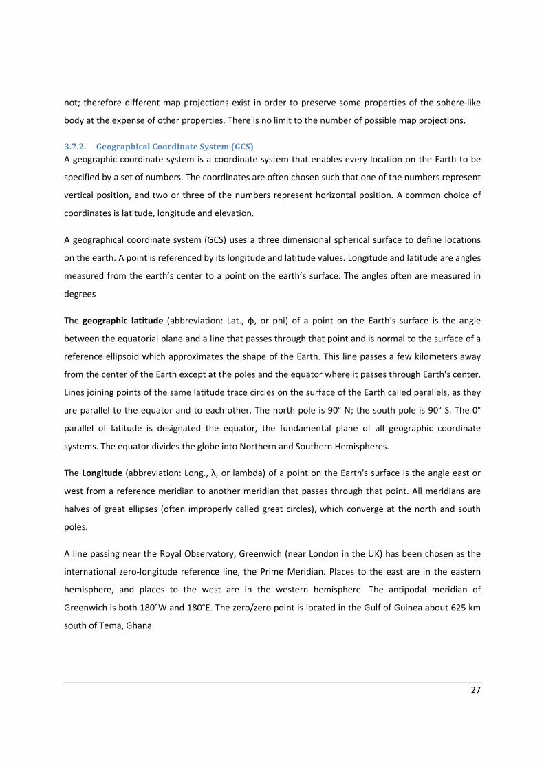
3.7.2. Geographical Coordinate System (GCS)
A geographic coordinate system is a coordinate system that enables every location on the Earth to be
specified by a set of numbers. The coordinates are often chosen such that one of the numbers represent
vertical position, and two or three of the numbers represent horizontal position. A common choice of
coordinates is latitude, longitude and elevation.
A geographical coordinate system (GCS) uses a three dimensional spherical surface to define locations
on the earth. A point is referenced by its longitude and latitude values. Longitude and latitude are angles
measured from the earth’s center to a point on the earth’s surface. The angles often are measured in
degrees
The geographic latitude (abbreviation: Lat., φ, or phi) of a point on the Earth's surface is the angle
between the equatorial plane and a line that passes through that point and is normal to the surface of a
reference ellipsoid which approximates the shape of the Earth. This line passes a few kilometers away
from the center of the Earth except at the poles and the equator where it passes through Earth's center.
Lines joining points of the same latitude trace circles on the surface of the Earth called parallels, as they
are parallel to the equator and to each other. The north pole is 90° N; the south pole is 90° S. The 0°
parallel of latitude is designated the equator, the fundamental plane of all geographic coordinate
systems. The equator divides the globe into Northern and Southern Hemispheres.
The Longitude (abbreviation: Long., λ, or lambda) of a point on the Earth's surface is the angle east or
west from a reference meridian to another meridian that passes through that point. All meridians are
halves of great ellipses (often improperly called great circles), which converge at the north and south
poles.
A line passing near the Royal Observatory, Greenwich (near London in the UK) has been chosen as the
international zero-longitude reference line, the Prime Meridian. Places to the east are in the eastern
hemisphere, and places to the west are in the western hemisphere. The antipodal meridian of
Greenwich is both 180°W and 180°E. The zero/zero point is located in the Gulf of Guinea about 625 km
south of Tema, Ghana.

28
Representation of Earth Latitude and Longitude
3.7.3. Spheroids, Spheres & Datum
While a spheroid approximates the shape of the earth, a datum defines the position of the spheroid
relative to the center of the earth. A datum provides a frame of reference for measuring locations on
the surface of the earth. It defines the origin and orientation of latitude and longitude lines.
Sphere and spherioid Datum
3.7.4. Geodetic datum
A geodetic datum (plural datums, not data) is a reference from which measurements are made. In
surveying, a datum is a set of reference points on the Earth's surface against which position
measurements are made, and (often) an associated model of the shape of the earth (reference ellipsoid)
to define a geographic coordinate system. Horizontal datums are used for describing a point on the
earth's surface, in latitude and longitude or another coordinate system. Vertical datums measure
elevations or depths.
A reference datum is a known and constant surface which is used to describe the location of unknown
points on the earth. Since reference datums can have different radii and different center points, a
specific point on the earth can have substantially different coordinates depending on the datum used to
make the measurement. There are hundreds of locally-developed reference datums around the world,

29
usually referenced to some convenient local reference point. Contemporary datums, based on
increasingly accurate measurements of the shape of the earth, are intended to cover larger areas.
Geodetic datum defines the size and shape of the earth, and the origin and orientation of the coordinate
systems used to map the earth. Reference surface used for map projections. Several models of geodetic
datums in use: eg. Everest ellipsoid, WGS84
Indian Standard is EVEREST ELLIPSOID. World Standard is WGS84 ELLIPSOID
3.7.5. The Universal Transverse Mercator (UTM)
The Universal Transverse Mercator (UTM) geographic coordinate system uses a 2-dimensional Cartesian
coordinate system to give locations on the surface of the Earth. It is a horizontal position representation,
i.e. it is used to identify locations on the earth independently of vertical position, but differs from the
traditional method of latitude and longitude in several respects.

30
The UTM system is not a single map projection. The system instead divides the Earth into sixty zones,
each a six-degree band of longitude, and uses a secant transverse Mercator projection in each zone.
3.7.6. World Geodetic System
The World Geodetic System is a standard for use in cartography, geodesy, and navigation. It comprises a
standard coordinate frame for the Earth, a standard spheroidal reference surface (the datum or
reference ellipsoid) for raw altitude data, and a gravitational equipotential surface (the geoid) that
defines the nominal sea level. WGS 84 is the reference coordinate system used by the Global Positioning
System.
3.8. Projected Coordinate Systems
A Projected Coordinate System is defined on a flat, two-dimensional surface. It has constant lengths,
angles, and areas across the two dimensions. It is always based on a geographic coordinate system that
is based on a sphere or spheroid.
Map projections can lead to distortions.
Conic Projection
• The most simple conic projection is tangent to the globe along a line of latitude. This line is
called the standard parallel. The meridians are projected onto the conical surface, meeting at
the apex, or point, of the cone.
• Parallel lines of latitude are projected onto the cone as rings.

31
• The cone is then ‘cut’ along any meridian to produce the final conic projection, which has
straight converging lines for meridians and concentric circular arcs for parallels. The meridian
opposite the cut line becomes the central meridian.
Cylindrical projections
• Meridians are geometrically projected onto the cylindrical surface, and parallels are
mathematically projected. This produces graticular angles of 90 degrees. The cylinder is ‘cut’
along any meridian to produce the final cylindrical projection. The meridians are equally spaced,
while the spacing between parallel lines of latitude increases toward the poles
Planar projections
Planar projections project map data onto a flat surface touching the globe. A planar projection is also
known as an azimuthal projection or a zenithal projection.

32
• The Gnomonic projection views the surface data from the center of the earth,
• The Stereographic projection views it from pole to pole.
• The Orthographic projection views the earth from an infinite point, as if from deep space
BEHRMANN EQUAL AREA CYLINDRICAL projection
Shape: Shape distortion is minimized near the standard parallels (30N and 30S).
Area: Area is maintained.
Direction: Directions are generally distorted.
Distance: Directions are generally distorted except along the equator.
USES AND APPLICATIONS: Only useful for world maps
Top Related