1 Meshless method theory

One of the reasons for this development is the fact that mesh-free and mesh-adaptive discretizations are oftenbetter suited to cope with geometric changes of the domain of interest, e.g. free surfaces and large deforma-tions, than the classical structured-mesh discretization techniques(FEM-finite element method, FDM-finitedifference method, FVM-finite volume method etc). Typically, more than 70 percent of the overall comput-ing time is spent by mesh generators. Since mesh-free discretization techniques are based only on a set ofindependent points which eliminates the costs of mesh generation. The classical FEM relies on the localapproximation properties of polynomials. The method fails when there is high local oscillatory solution orhigh deformation locally. This can also be understood as that there is a need of high Ck continuity func-tions( p-refinement) in the FEM literature. Meshless method provides the good solution for this p-refinementproblem of FEM with the help of shape functions called Kernel functions without increasing the cost of thesolution, and while keeping the reasonable degree of accuracy. Meshless method shape functions has moresmoothness which means that one can go to higher order derivative also.

Several meshfree methods have been proposed since the prototype of the meshfree methods(the smoothedparticle hydrodynamics (SPH) by Gingold and Monaghan [21] and L. B. Lucy[30]) was born. They are thediffuse element method (DEM) by Nayrole et al. [33], the element free Galerkin method(EFG) by Belytschkoet al. [8], the reproducing kernel particle method (RKPM) by Liu et al. [28], the partition of unity finiteelement method (PUFEM) by Babuska and Melenk [4], the h-p Clouds by Duarte and Oden [14], the movingleast-square reproducing kernel method(MLSRK) by Liu et al. [29], the meshless local boundary integralequation method (LBIE)by Zhu et al. [49], the meshless local PetrovGalerkin method (MLPG) by Atluri etal. [2], meshless point collocation methods by Aluru [1], meshless finite point method by Onate et al.[34]and more.

The development of this method is motivated by the need for new techniques for the solution of problemswhere the classical FEM approaches fail or are prohibitively expensive; for example, equations with roughcoefficients(arising e.g. in the modelling of composites, materials with microstructure, stiffeners, etc) andproblems with boundary layers or highly oscillatory solutions fall into that category.

2 SPH

In the traditional SPH method proposed by Gingold and Monaghan [21], the state of the art is representedby a set of particles which possess individual material properties and move according to the governing con-servation equations i.e equilibrium equation. Smoothed particle hydrodynamics, as a meshfree, Lagrangian,particle method, has its particular characteristics. It has some special advantages over the traditional grid-based numerical methods, the most significant one among which is the adaptive nature of the SPH method.This adaptability of SPH is achieved at the very early stage of the field variable approximation that is per-formed at each time step based on a current local set of arbitrarily distributed particles or in other wordswith the help of kernel function of compact support which make sure that the value at any particle is con-sistent with the neighbouring particles within the compact support. Because of this adaptive nature of theSPH approximation, the approximation is not affected by the arbitrariness of the particle motion. Therefore,it can naturally handle problems with extremely large deformation. This is, therefore, the most attractivefeature of the SPH method. SPH is derived in two step process: first the kernel approximation and thesecond is particle approximation as mention below. Theoretically exact value of any generic function at anypoint can be computed by taking the convolution of the function with dirac function.

f(x)|I =∫

Ω

f(x)δ(x− xI)dΩ (1)

1

The dirac delta function can be loosely thought of as a function on the real line which is zero everywhereexcept at the point location xI , where it is infinite

δ(x− xI) =∞, x = xI

0, x 6= xI(2)

and which is also constrained to satisfy the identity∫ ∞−∞

δ(x)dx = 1 (3)

Since the dirac function is hypothetical function, and its difficult to talk about its continuity and differentia-bility at any point. Therefore there is a need which can substitute well the dirac function. In the same spirit,the first approximation is introduced by using the smoothed function WI(x), also called Kernel function inplace of dirac function.

fh(x)|I =∫

Ω

f(x)W (x− xI , h)dΩ (4)

where h is called the smoothing length of the kernel function. The kernel function are compact in naturewhich means that they are non zero positive in small domain while zero elsewhere. The smoothing lengthgoverns the shape and the amplitude of the kernel function. When the smoothing length h → 0 the kernelcan be approximated by the Dirac delta function.

limh→0

W (x, h) = δ(x) (5)

The second approximation called particle approximation is employed at this stage to solve the above(eq. 4) numerically, which is being used in computational analysis. This can be achieved by discretizationof the continuous domain Ω into the small patches ∆ΩJ as

fh(x)|I =∑

J

fJWI(xJ)∆ΩJ (6)

In the similar way the approximation of the gradient of the generic function f(x) is derived. For examplereplacing the function f(x) in (eq. 4) by ∇f(x) can be represent as

∇fh(x)|I =∫

Ω

∇f(x)W (x− xI , h)dΩ (7)

By applying the integration by parts, above equation can be rewritten as

∇fh(x)|I =∫

∂Ω

f(x)W (x− xI , h)nd∂Ω−∫

Ω

f(x)∇W (x− xI , h)dΩ (8)

Due to the compact support property of the choosed kernel function, the first term of the right handside approaches to zero. But this term will not tends to zero when the particle location is on the boundaryor near boundary of the domain. Moving from (eq. 1) to (eq. 6) reproducibility is lost. This deficiency hasimportant consequences for the resolution of boundary value problems in terms of accuracy, stability and

2

convergence of the approximation[42].This convergence problem will be addressed later in this report. Nowfurther with the help of the second approximation, we can rewrite the equation as,

∇fh(x)|I = −∑

J

fJ∇WI(xJ)∆ΩJ (9)

But due to the convergence reason for the non-uniform particle distribution, the equation is modified tothe following

∇fh(x)|I =∑

J

[fI − fJ ]∇WI(xJ)∆ΩJ (10)

which adds one more property of the suitable kernel function should meet that the derivative of the kernelfunction is anti-symmetric in the domain at about any point location or mathematically by saying

∫Ω

∇WI(xJ)dΩ = 0 (11)

In particular, SPH methods are widely used for fast transient dynamic simulations, such as explosionsor impact problems, because of their low computational cost and its ability to handle severe distortions.Other meshless methods, such as EFG or RKPM, can also deal with large distortions and go beyond finiteelement computations, but with a higher computational cost(due to the use of Gauss quadratures or specifictechniques to accurately integrate the weak form). In its original form SPH had several weak points, describedin detail in Swegle et al. [43]and Belytschko et al. [6] and Xiao et al. [46], and also Huerta et al. [24] for areview. These problems listed as:

1. Lack of Consistency or completeness [7].

2. Tensile instability [46, 43, 15].

3. Applying essential boundary conditions.

4. Presence of zero-energy modes or the oscillatory modes in the numerical solution[46].

Some of the measures proposed in literature to cure these drawbacks are re-mentioned here in this worklater.

2.1 Kernel Functions

Since the kernel is the key element in the SPH methodology, this should be primary concern to any user ofSPH. In the paper[20] analyzed the measures of merit for one-dimensional SPH kernel functions. Variouskernels with a compact support have been established[20], such as super Gaussian kernels, spline kernels ,polynomial kernels and cosine kernels etc. The computational range of these kernels is usually no more thanthree times the smoothing length. Its concluded there that the key variables in a kernel’s worth is its shapeand the ration of the particle separation with respect to smoothing length, ∆x/h. Its being approved thatbell shaped kernel functions (Gaussian kernel functions) and Q-spline kernels can be regarded as the bestkernels [20, 23] in approximation as compared to other kernel functions. Kernel function should try to meetthe same properties as the dirac function listed below.

3

• Positive in its domain

• Integral of the kernel over entire domain is equal to one,∫

ΩWi(x)dΩ = 1

• Continuous higher derivatives.

• Defined in compact support

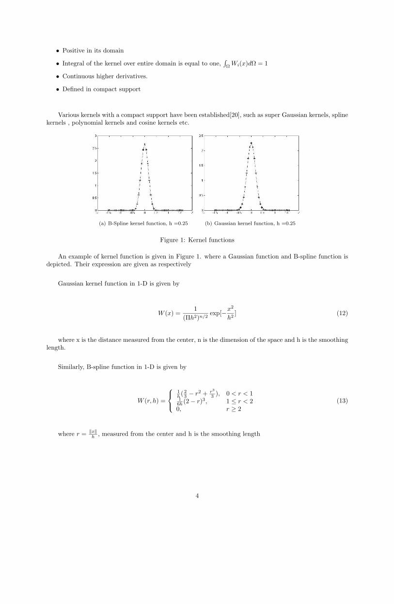
Various kernels with a compact support have been established[20], such as super Gaussian kernels, splinekernels , polynomial kernels and cosine kernels etc.

(a) B-Spline kernel function, h =0.25 (b) Gaussian kernel function, h =0.25

Figure 1: Kernel functions

An example of kernel function is given in Figure 1. where a Gaussian function and B-spline function isdepicted. Their expression are given as respectively

Gaussian kernel function in 1-D is given by

W (x) =1

(Πh2)n/2exp[−x

2

h2] (12)

where x is the distance measured from the center, n is the dimension of the space and h is the smoothinglength.

Similarly, B-spline function in 1-D is given by

W (r, h) =

1h ( 2

3 − r2 + r3

3 ), 0 < r < 11

6h (2− r)3, 1 ≤ r < 20, r ≥ 2

(13)

where r = ‖x‖h , measured from the center and h is the smoothing length

4

3 Consistency, Completeness and reproducing conditions

In the finite-difference literature the consistency of an approximation is defined by its ability to exactlyrepresent the differential equation in the limit as the number of grid points goes to infinity and the maximumdistance between neighbouring grid points goes to zero. Consistency plus stability implies convergence. . Asmentioned before moving from (eq. 1) to (eq. 6) reproducibility is lost, and there is great need of correctingthe kernel functions of traditional SPH to meet the convergence criterion at the boundary. Two types ofcorrection are proposed in literature. We can employ correction either to the approximating functions, or tothe derivatives in order to have the completeness of the approximating functions.

An approximation fh(x) is complete to order k if any polynomial up to order k can be representedexactly.

fh(x) =∑

I

ΦI(x)fI (14)

where ΦI(x) are approximating functions and fI are the nodal values. If the nodal values are given by apolynomial, i.e

fI = a0 + a1xI + a2x2I + . . .+ akx

kI (15)

then the reproducing conditions(and completeness)of order k are met if

fh(x) =∑

I

ΦI(x)fI = a0 + a1x+ a2x2 + . . .+ akx

k (16)

By the above equation we can obtain the following conditions

∑I

ΦI = 1 (17)

∑I

ΦIxI = x (18)

∑I

ΦIx2I = x2 (19)

. . . ∑I

ΦIxkI = xk (20)

As proposed in the literature that we can employ correction to the derivative also for reproducing theapproximating functions completely. Computationally the cost for the corrected derivative is less as comparedto the corrected approximating function for reproducing the functions completely. This can be obtained bytaking the derivatives of above equations. For example, the linear derivative reproducing conditions forfunctions in 1D can be written as

5

∑I

ΦI,x = 0 (21)

∑I

ΦI,xxI = 1 (22)

For correction of the approximating function, some following approaches are proposed. In the bracket it ismentioned the order of the polynomial that the following correction can able to reproduce exactly.

1. Shepard Correction.[41] (constant functions only)

2. Moving least square approach.[27](desired kth order function)

3. Reproducing kernel particle approach.[27](desired kth order function)

4. Radial basis function.

We can also employ the derivative corrections to reproduce function completely. Several approaches areexamined with some mentioned below:

1. Symmetrization given in Monaghan.[32]

2. Johnson and Beissel Correction.[25](linear functions)

3. Randles and Libersky renormalization.[40](constant or linear functions)

4. Krongauz and Belytschko correction.[26](linear functions)

3.1 Correction of approximating function

The first approach to insuring completeness in kernel approximations is to correct the approximation functionso that it satisfies the required reproducing conditions. After the correction is make on the approximation, thederivatives of the approximation will satisfy the corresponding derivative reproducing conditions. Expandingthe Taylor series for f(x) about xI , and multiplying both sides by a kernel function, and integrating overthe domainΩ yields,

∫Ω

f(x)WI(x)dx =f(xI)∫

Ω

WI(x)dx+ fx(xI)∫

Ω

(x− xI)WI(x)dx

+ fxx(xI)∫

Ω

(x− xI)2WI(x)dx+ . . .

(23)

where fx = dfdx ,fxx = d2f

dx2 , and WI(x) = W (x−xI , h). By the symmetry property of the kernel function,coefficients of the first derivative terms on the right side of the above equation tends to zero, except nearthe boundary, which means the following at the boundary,

6

∫Ω

(x− xI)WI(x)dx ∼=∫

Ω

Θ(h)WI(x)dx∫Ω

(x− xI)2WI(x)dx ∼=∫

Ω

Θ(h2)WI(x)dx(24)

The above equations can be corrected so that it tends to zero by making correction to the kernel functionor in other words make the inherent property of the choosed kernel function.

Therefore the (eq. 23) can be rewritten as by dropping the truncation error terms (eq. 24),

f(x)I∼=∫

Ωf(x)WI(x)dx∫

ΩWIdx

(25)

For those points xI far away from a boundary, the integral of WI(x) is equal to 1. Hence, (eq. 25) reducesto the conventional kernel estimate, (eq. 6). The truncation error is on the order of (x − xI)2 or h2 in theinterior of the domain whereas on the order of (x − xI) or h for xI near or on the boundary because theintegral of the product (x − xI)WI(x) is no longer equal to zero. The difference between (eq. 4) and (eq.25) is clear. Ignoring the correction term (denominator term), i.e. the integral of WI(x) in (eq. 25), is theessential factor for causing the boundary deficiency in the conventional kernel estimate. In the similar way,we can approach to the correction of the derivative of the approximating function by replacing WI(x) withWI,x = ∂WI(x)

∂x . The following expression is generated by manipulation of the (eq. 23)

f(x)I∼=∫

Ω[f(x)− f(xI)WI,xdx∫

Ω(x− xI)WI,xdx

(26)

Since by the property of the kernel function that the first derivative of the kernel function is antisymmetric,denominator of the (eq. 26) will not become zero. The truncation error is of order of h2 in the interiordomain and of order h near the boundary. The following section mention the two general approach forcorrecting the approximating function to the desired kth order reproducibility.

3.1.1 Moving Least Square approach

Moving least square is the approach to achieve the corrected kernel function. Moving least square is the sim-ilar term that is used in Statistics to fit the curve among the scattered data points. Assume the interpolatingfunction fh(x) in the form

fh(x) = fh(x, a0, a1, . . . , aI) (27)

where the parameters a0, . . . , aI are determined by minimizing the error.( for each fixed x; therefore, strictlyspeaking, the coefficients depend on x). The local character of the moving least-squares (MLS) approxima-tion, i.e. the moving part, arises from the dependence of parameters aI on x which further depends on thekernel window.

L = ΣI [fI − fh(xI , a0 . . . , aI)]2WI(x) (28)

This method is called moving least squares method. By minimization of the above equation, the parametersare determined, and the global approximation fh(x) takes the form

fh(x) = ΣIΦI(x)fI (29)

Construction: In the moving least square approximation, we let

fh(x) =∑

I

pI(x)aI(x) (30)

7

Here I is the number of terms in the basis, pI(x) are monomial basis functions, and aI(x) are theircoefficients, which as indicated, are functions of the spatial coordinates x. The commonly used bases for thelinear and quadratic basis in 1-D are

pT = (1, x) pT = (1, x, x2) in 1D, (31)

The coefficients aI(x) are obtained by minimizing the difference between the local approximation valueand the function value at any given point. This yields the quadratic form

J =∑

J

W (x− xJ)(fh(x, xJ)− f(xJ))2

=∑

J

W (x− xJ)[∑

I

pI(xJ)aI(x)− fJ ]2(32)

where W (x − xJ) is a weighting function with compact support; the same weight functions as in SPHare used. Note that the term corresponding to fh(x) in (eq. 32) consists of the monomials at xJ and thecoefficient at x Above equation can be rewritten in the form as

J = ((Pa− u)TW(x)(Pa− u) (33)

where fT = (f1, f2 . . . fn) = uT = (u1,u2 . . .un). The change of symbol is used here just for brevity.

P =

p1(x1) p2(x1) . . . pm(x1)p1(x2) p2(x2) . . . pm(x2)

......

. . ....

p1(xn) p2(xn) . . . pm(xn)

(34)

and

W(x) =

W (x− x1) 0 . . . 0

0 W (x− x2) . . . 0...

.... . .

...0 0 . . . W (x− xn)

(35)

To find the coefficients a(x), we obtain the extremum of J by

∂J

∂a= A(x)a(x)−B(x)u = 0, (36)

where B is called the moment matrix and is given by

A = PTW(x)P (37)

B = PTW(x) (38)

The approximation fh(x) can then be expressed as

fh(x) =∑

J

ΦkJ(x)fJ , (39)

8

where the shape functions are given by

Φk = [Φk1(x) . . .Φk

n(x)] = pTA−1(x)B(x), (40)

where the superscript k is the order of the polynomial basis. The above ΦkJ(x) are the corrected kernel

function of the consistency or reproducibility of order k. The spatial derivatives of the shape functions areobtained by

ΦI,x = (pTA−1BI),x

= pT,xA

−1BI + pT(A−1),xBI + pTA−1BI,x

(41)

whereBI,x =

dw

dx(x− xI)p(xI) (42)

and A−1,x is computed by

A−1,x = −A−1A,xA−1 (43)

where

A,x =n∑

I=1

w(x− xI)p(xI)pT(xI)

=dw

dx(x− x1)

[1 x1

x1 x21

]+dw

dx(x− x2)

[1 x2

x2 x22

]+ . . .

dw

dx(x− xn)

[1 xn

xn x2n

] (44)

Similarly, the second derivative expression can be derived by chain rule

(ΦI,x),x =(pT,x),xA−1BI),x + pT

,x(A−1),xBI + pT,xA

−1BI,x

pT,x(A−1),xBI + pT((A−1),x),xBI + pT(A−1),xBI,x

pT,xA

−1BI,x + pT(A−1),xBI,x + pTA−1(BI,x),x

(45)

where

(A−1,x),x = −(A−1A,xA−1),x

= −(A−1),xA,xA−1 −A−1(A,x),xA−1 −A−1A,x(A−1),x

(46)

9

3.1.2 Reproducing kernel particle approach

Reproduce Kernel approach was developed by Liu et al. [28] in order to reproduce the approximatingfunction correctly. By introducing the correction function, the kernel function in kernel estimate is modifiedto satisfy the consistency condition in any arbitrary domain of problems and, as a result, the shape functionof the method and its derivatives are derived.

It involves the correction to the kernel function as

KI(x) = CI(x)WI(x) (47)

In the above expression WI(x) is the SPH kernel function, while CI(x) function is the correction function.In order to obtain the desired reproducing properties CI(x) assumes the following relationship

CI(x) = b0I + b1I(x− xI) + . . . (48)

As mentioned in the section 3.1, the truncation error can be pushed to higher order terms if the choosedkernel function posses the following property.

p0 =∫

Ω

KI(X)dx = 1 (49)

p1 =∫

Ω

(x− xI)KI(X)dx = 0 (50)

p2 =∫

Ω

(x− xI)2KI(X)dx = 0 (51)

The above equation can be rewritten again with the help of the (eq. 48) as following considering theconsistency only upto first order term.

p0 =∫

Ω

(b0I + b1I(x− xI))WI(X)dx = 1 (52)

p1 =∫

Ω

(x− xI)(b0I + b1I(x− xI))WI(X)dx = 0 (53)

Further defining the following in the discretized form,

m0 =∑

J

WI(xJ)dxJ (54)

m1 =∑

J

(xJ − xI)WI(xJ)dxJ (55)

m2 =∑

J

(xJ − xI)2WI(xJ)dxJ (56)

Then, the following system of equation is obtained from (eq. 52-53)

10

b0Im0 + b1Im1 = 1b0Im1 + b1Im2 = 0

(57)

Solving for b0I , b1I from the above equations and back substitution to the (eq. 47) will give the requiredcorrected kernel function of first order consistency.

The basic idea of meshless methods[42] is to use shape functions which are used in fitting of points.More precisely, given a distribution of nodes xI , the fitting algorithm (moving least square or reproducingkernel approximant ) is invoked to produce to produce the shape functions, ΦI which are then used in thediscretization of the continuum in either method Galerkin or Collocation method. These shape functionsare used in a Galerkin or collocation discretization process to set up a linear system of equations. All thesedata fitting approaches do not depend (at least to a great extent)upon a mesh or any fixed relation betweengrid points (particles). However, the realization and implementation of such a method is not so simple ingeneral: there are often problems with stability and consistency conditions.

4 Discretization

The discretization scheme employed in the meshfree numerical simulation is presented in this section. In thework reported so far, the following method of discretization schemes are well renowned, namely

1. Collocation methods [1]

2. Galerkin methods [8, 37, 17]

3. Mixed Galerkin-Collocation methods.[11]

Each methods has some advantages and disadvantages in itself. Galerkin-based meshless method arecomputational intensive, whereas collocation-based meshless methods suffer from instability(Tensile insta-bility and rank deficiency). Lets consider the example of imposing collocation method and Galerkin methodson the conservation of linear momentum equation in Lagrangian formulation.

ρ0u = ∇X · P + ρ0b (58)

where ρ0 initial densities, u material time derivatives of displacment vector,∇X is the gradient or diver-gence operator expressed in material derivatives, P is the nominal stress tensor and b is the body force. Theboundary conditions are following

u(X, t) = u(X, t) Γu0 (59)

n0 ·P(X, t) = t(X, t) Γt0 (60)

where u and t are the prescribed displacement and traction values on the boundary, respectively, n0 is theoutward normal to the domain and Γu

0 ∪ Γt0 = Γ0, Γu

0 ∩ Γt0 = 0

11

4.1 Collocation Based Method

In collocation methods the discrete equations are obtained by enforcing the equilibrium equation on the setof nodes. Now by enforcing the kernel approximation mentioned in (eq. 9) to the governing (eq. 58) atparticle I in domain is represented as

ρ0uI =∑

J

∇XWIJ · PJ∆ΩJ + ρ0b (61)

The above equation are simply linear algebraic equation system and could be solved by any of the stan-dard methods. It should me noted that some more algebraic linear system equations comes from boundaryconditions. Hence in this method there are more number of equations than actually the number of unknowns.Nodal integration is used to solve the above equation which encompasses instability due to rank deficiencyand tensile instability. Stress point integration could be used to remove rank deficiency, but tensile instabilitycould not be eliminated [46].

As an attempt to avoid the weak form Galerkin method, a least-square formulation was suggested [38] butproved to be adequate only for lower-order schemes such as those for first-order partial differential equations.As an alternative approach, Onate et al. [35] developed a point collocation scheme for fluid flow problem onthe basis of weighted least-squares procedure, which they called the finite point method. The finite pointmethod includes additional terms in the strong form to stabilize the convective term. Onate et al. [36]also applied this method to elasticity problems. Aluru [1] and Zhang et al. [48] presented point collocationmethods based on the reproducing kernel approximation and radial basis functions, respectively. Zhang etal. [47] proposed a least-squares collocation meshfree method which uses auxiliary points to improve thesolution accuracy.

4.2 Galerkin Based Method

Galerkin Based formulation is the standard method that is used in FEM formulation also. One of the essentialingredient of the Galerkin formulation is the integration by parts and the application of the divergencetheorem. Using the same idealogy (eq. 58) can be framed in galerkin method as

∫Ω0

ρ0δu · udΩ =∫

Ω0

ρ0δu · bdΩ−∫

Ω0

(∇Xδu)T : PdΩ +∫

Γ0

δu · tdΓ (62)

where δu is the test function from its right candidate Hilbert space set which is here in this case thesubset of corrected Kernel functions. Now imposing corrected SPH approximation to the above equationwill give

mI uI = fextI − f int

I , (63)

fextI =

∫Ω0

ρ0WIbdΩ +∫

Γ0

WItdΓ (64)

12

f intI =

∫Ω0

(∇XWI)T · PdΩ (65)

Galerkin methods require some type of cell structure for integration over the problem domain. Thisprocedure assumes exact integration and thus inaccuracy in the integration is directly related to the solutionaccuracy. Although Galerkin-based meshfree methods have advantageous features, difficulties of imposingessential boundary conditions and undeniable usage of background cell for Galerkin formulation erode meritsof meshfree methods. Nodal integration, cell or octree quadrature, and background finite element meshquadrature have been used. The first of these is the fastest, but appears to suffer from instability [5]and several stabilization schemes have been developed. The second and third have the disadvantage thatthe resulting method is not truly meshless. In Galerkin based meshless method (GBMM), derivatives indomain integrals are lowered by using the divergence theorem to establish the weak form. The inaccuracy inintegration will result in significant error in the solution. However, the shape functions in meshless methodare very complex. Delicate background cells and a large number of quadrature points must generally beemployed to integrate the weak form as accurate as possible. As a consequence, the GBMM is much moreexpensive than FEM.

4.3 Integration Schemes

The computational efficiency of mesh free Galerkin methods hinges critically on the choice of domain quadra-ture, and the issue is more computationally critical in fast dynamics and iterative equilibrium. The shapefunctions in meshfree methods are rational functions of the spatial coordinates and their local supports maynot align with the integration domains. This misalignment is the more significant source of error and affectsthe accuracy and convergence of meshfree methods[13]. The article [13]also proposes the technique boundingbox to impose the alignment of the kernel supports with the integration domain. Note that in case of FEMssupports and integration domains always coincide. Accurate integration of the weak form requires for morequadrature points than in finite element methods. Hence the computational demand of mesh free methodsto employ quadrature rules is quiet high as compared to FEMs. The major issues with discretization ofthe continuum via Galerkin is the evaluation of the integrals of the eq. 61 and eq. 64-65. There has someproposed approaches mentioned here.

1. Nodal integration , where the integral is evaluated by

∫Ω

f(x)dΩ =n∑

I=1

f(xI)∆ΩI (66)

This is the nodal integration scheme[17] posses the same stability properties as of SPH, which is truelymeshless method. The nodal integration is used in collocation methods for evaluating the integrals term.Though this integration is very fast and most suitable e.g for fast transient dynamics problems but thisapproach gives unstable results for integrating higher order differential equation i.e second order orhigher. This need the further careful study for this instabilities which is also not much touched part inthe literature. Quadrature schemes that employ only the nodes (also called the particles) as quadraturepoints, are only moderately slower than the FEM; however, they tend to exhibit instabilities[6, 39].This problem has been addressed by Beissel and Belytschko [5] and Chen et al. [10], where least-squares stabilization for nodal integration is proposed. Nevertheless, many remarkable solutions havebeen obtained by standard SPH.

2. Cell or octree quadrature where a regular array of domains in the background is used for quadra-ture. This approach cost more than the finite element method computationally because the mesh freeapproximants are non-polynomial in character and required more integration points.

13

3. Stress point integration approach.

Actually its not the new approach but a remedy proposed by Dyka et al. [15, 16] to stabilize thestandard SPH method or nodal integration method. The convergence and stability properties ofstress-point integration are between full integration and nodal integration; the later can be consideredunstable. The numerical studies that for uniform arrangements of particles, stress point integrationachieves good convergence rates. However, for non-uniform arrangements of particles fail to converge.Least square stabilization is used with stress point integration to get more stabilization and convergencefor non-uniform arrangement of particles[19]. Randles et al. [40] extended stress point integrationto higher dimensions to stabilize the normalized form of SPH. Stress point integration eliminatesinstabilities due to rank deficiency but not those due to the tensile instability, see Belytschko et al.[46]. Stress point integration is used when nodal integration is employed either in collocation methodor Galerkin method for removing spurious modes or oscillatory modes (rank deficiency instability).This is used only in evaluating the internal force term. eq. 65 can be represented as the following usingextra integration points called stress points by

f intI =

∑J1

V 0J1∇XWI(XJ1) · PJ1 +

∑J2

V 0J2∇XWI(XJ2) · PJ2 (67)

where J1 and J2 are subsets of master nodes and stress points respectively.

In the second and third cases Gauss quadratures or specific techniques are employed to accuratelyintegrate[42] the weak form. In the EFG method, the integrals of eq. 64-65 are usually evaluated overbackground cells based on an octree structure. Full quadrature in the cells is computationally expensive fornonlinear and or dynamic problems. SPH collocation is equivalent to EFG method when nodal integrationstrategy is employed, so it will exhibit the same instabilities.

5 Boundary Conditions

Imposing essential boundary conditions is a key issue in mesh-free methods. The shape functions in meshlessmethods are not strict interpolants, i.e they do not satisfy the Kronecker delta condition

NA(xB) 6= δAB 6=

1 ifA = B0 otherwise

(68)

where NA(xB) is the shape function of node A evaluated at node B, and δAB is the Kronecker delta. Inother words the shape function associated to a particle does not vanish at other particles, which is not thecase with Finite element method. A consequence of this is that the approximated value on the boundarydepends on interior nodes as well as boundary nodes. For example this prevents the treatment like finiteelement method for Dirichlet boundary conditions, where boundary nodes are simply omitted from thesolution procedure. Some of the proposed technique for implementing the essential boundary conditions inmesh free methods are mentioned. These techniques can be classified in following groups:

1. methods based on a modification of the weak form, such as Lagrange multiplier method[8], the penaltymethod [49]and Nitsche’s method[22, 3]

2. methods in which coupling is achieved between the meshfree shape functions and the finite elementshape function near the boundary, which allows directly to impose prescribed values. Coupling betweenFE and SPH [31]or between FE and EFG or RKPM [9, 24]is used to deal with boundary conditions

14

problem. On the other hand, bridge scale method proposed in [44] is a general technique to mix amesh-free approximation with any other interpolation space, in particular with finite elements near theessential boundary.

The most excellent review for imposing the boundary conditions in mesh free method could be found in[18].

6 Stability and Convergence of Meshfree methods

The stability of the particle (meshfree ) method is essential to their robustness. Three kinds of instabilitiesmainly results from the discretization of the continua are mentioned in literature so far namely:

1. a high frequency instability which results from the rank deficiency of the discrete divergence operatorand makes the equilibrium equations singular; this occurs regardless of the value of the stress.

2. a tensile instability which results from the interaction of the second derivative of kernel and the tensilestress, it occurs even in one-dimensional plane response or also defined premature fragmentation of theSPH grid in tension.

3. Material instability which is also found in continua.

The tensile instability was first identified by Swegle et al. [43] by a Neumann analysis of the one-dimensional equation. This behavior is synonym to the under-integration of the Galerkin form which leadsto spurious singular modes( also called node to node oscillation in some of the reviews) in the solution space.This is analogous to hourglass control for reduced integration in finite element techniques. Stability is aprimary concern for any nodal integration method since large oscillations in the solution can often occurunless some measures are taken to mitigate them. In lieu of stabilization, stress points are often introducednear the nodes to avoid these oscillations.

Stress-point integration was first proposed by Dyka and Ingel [15] and Dyka et al. [16] for tensioninstabilities in SPH. In fact, stress points do not suppress tension instabilities, which are due to a ratheranomalous description of the motion in SPH, see [6]. Instead, in many cases they restore the positive definite-ness of the linear equations, i.e. they correct rank deficiency. Stress-point integration for multi-dimensionswas proposed by Randles et al.[40], who use only the stress points for quadrature. The convergence andstability properties of stress-point integration are between full integration and nodal integration; the lattercan be considered unstable.

Some review is mentioned in the article[6] regarding the stability analysis of meshfree methods withEulerian and Lagrangian kernels formulation. It was concluded in the article that instability due to rankdeficiency occurs for both Lagrangian and Eulerian kernels with nodal integration or collocation. Thisinstability can be eliminated by stress points. However, it is found stress points cannot completely stabilizeEulerian kernels. It will be shown that the tensile instability is to a large extent the idiosyncrasy of what wecall Eulerian kernels. In an Eulerian kernel, the stability depends on the stress and the second derivative ofthe kernel. This generates the tensile instability. When the kernel is function of the material(Lagrangian)co-ordinates, a so- called Lagrangian kernel, the tensile instability does not occur. It was also concluded thatthe best approach to stable particle discretizations is to use Lagrangian kernels with stress points. Howeverthe convergence and stability depends on the distribution of the particles on the domain, which give verypoor convergence for non-uniform particle distribution. It was concluded that stability can be achieved in

15

irregular particle distribution by least-square stabilization. The following methods proposed so far in therealm for the stabilization of meshfree methods.

1. Swegle et al. [45] have proposed a conservative smoothing scheme to eliminate the tensile instability.

2. The short wave length modes can be suppressed with Least square stabilization [5, 10]for nodal in-tegration stability which contains the square of the residual of the momentum equation in the weakform.

3. Stabilization by stress point technique which suppresses high frequency instability.

7 Numerical Simulation

Some of the numerical simulation for the solution of the differential equationis presented in this section. Itshould be noted that Gaussian kernel, WI is used with smoothing length (h = 0.225)in all the examples. Thefollowing example illustrates the significance of the uncorrected and corrected standard SPH kernel functionin approximating the function. The following function is approximated by the standard SPH method.

f(x) = sinx 0 ≤ x ≤ Π (69)

The equations that are used in approximating the above function and its derivative are as.

fh(x)|I =∑

J

fJWI(xJ)∆ΩJ (70)

∇fh(x)|I =∑

J

[fI − fJ ]∇WI(xJ)∆ΩJ (71)

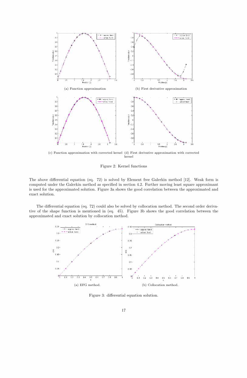
Figure 2.a-2.b clearly mention the inaccuracy in reproducing the function and its first derivative near theboundaries. After correcting the kernel function by Moving least square approach mentioned in section 3.1.1,Figure 2.c-2.d shows excellent correlation between the exact and approximated function.

7.1 Spatial differential equation

Consider the following one-dimensional second order differential equation on the domain 0 ≤ x < 1

d2u

dx2+ x = 0 (72)

with the following boundary conditions

u(0) = 0du

dx|x=1= 0

(73)

The exact solution to the above problem is given by

u(x) = (x

2− x3

6) (74)

16

(a) Function approximation (b) First derivative approximation

(c) Function approximation with corrected kernel (d) First derivative approximation with correctedkernel

Figure 2: Kernel functions

The above differential equation (eq. 72) is solved by Element free Galerkin method [12]. Weak form iscomputed under the Galerkin method as specified in section 4.2. Further moving least square approximantis used for the approximated solution. Figure 3a shows the good correlation between the approximated andexact solution.

The differential equation (eq. 72) could also be solved by collocation method. The second order deriva-tive of the shape function is mentioned in (eq. 45). Figure 3b shows the good correlation between theapproximated and exact solution by collocation method.

(a) EFG method. (b) Collocation method.

Figure 3: differential equation solution.

17

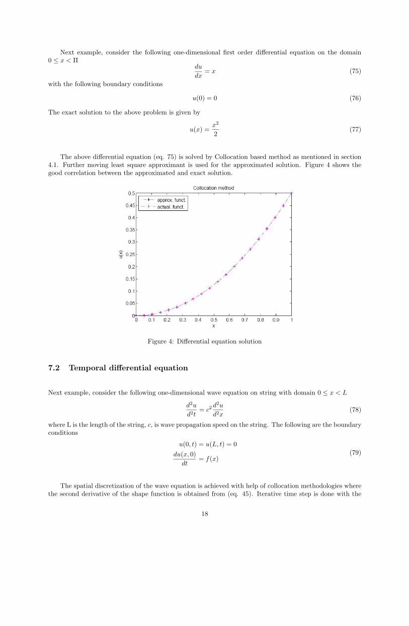
Next example, consider the following one-dimensional first order differential equation on the domain0 ≤ x < Π

du

dx= x (75)

with the following boundary conditions

u(0) = 0 (76)

The exact solution to the above problem is given by

u(x) =x2

2(77)

The above differential equation (eq. 75) is solved by Collocation based method as mentioned in section4.1. Further moving least square approximant is used for the approximated solution. Figure 4 shows thegood correlation between the approximated and exact solution.

Figure 4: Differential equation solution

7.2 Temporal differential equation

Next example, consider the following one-dimensional wave equation on string with domain 0 ≤ x < L

d2u

d2t= c2

d2u

d2x(78)

where L is the length of the string, c, is wave propagation speed on the string. The following are the boundaryconditions

u(0, t) = u(L, t) = 0du(x, 0)dt

= f(x)(79)

The spatial discretization of the wave equation is achieved with help of collocation methodologies wherethe second derivative of the shape function is obtained from (eq. 45). Iterative time step is done with the

18

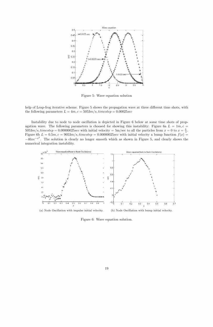
Figure 5: Wave equation solution

help of Leap-frog iterative scheme. Figure 5 shows the propagation wave at three different time shots, withthe following parameters L = 4m, c = 5053m/s, timestep = 0.00025sec

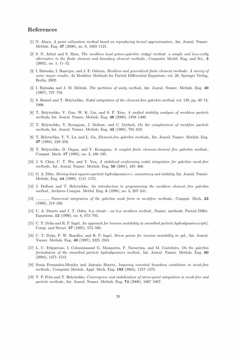
Instability due to node to node oscillation is depicted in Figure 6 below at some time shots of prop-agation wave. The following parameters is choosed for showing this instability: Figure 6a L = 1m, c =5053m/s, timestep = 0.00000025sec with initial velocity = 5m/sec to all the particles from x = 0 to x = L

4 .Figure 6b L = 0.5m, c = 9053m/s, timestep = 0.00000025sec with initial velocity a bump function f(x) =−40xe−x2

. The solution is clearly no longer smooth which as shown in Figure 5, and clearly shows thenumerical integration instability.

(a) Node Oscillation with impulse initial velocity. (b) Node Oscillation with bump initial velocity.

Figure 6: Wave equation solution.

19

References

[1] N. Aluru, A point collocation method based on reproducing kernel approximation., Int. Journl. Numer.Methds. Eng. 47 (2000), no. 6, 1083–1121.

[2] S. N. Atluri and S. Shen, The meshless local petrov-galerkin (mlpg) method: a simple and less-costlyalternative to the finite element and boundary element methods., Computer Model. Eng. and Sci., 3(2002), no. 1, 11–52.

[3] I. Babuska, I. Banerjee, and J. E. Osborn, Meshless and generalized finite element methods: A survey ofsome major results., In Meshfree Methods for Partial Differential Equations, vol. 26, Springer Verlag,Berlin, 2002.

[4] I. Babuska and J. M. Melenk, The partition of unity method., Int. Journl. Numer. Methds. Eng. 40(1997), 727–758.

[5] S. Beissel and T. Belytschko, Nodal integration of the element-free galerkin method, vol. 139, pp. 49–74,1996.

[6] T. Belytschko, Y. Guo, W. K. Liu, and S. P. Xiao, A unified stability analysis of meshless particlemethods, Int. Journl. Numer. Methds. Eng. 48 (2000), 1359–1400.

[7] T. Belytschko, Y. Krongauz, J. Dolbow, and C. Gerlach, On the completeness of meshfree particlemethods, Int. Journl. Numer. Methds. Eng. 43 (1998), 785–819.

[8] T. Belytschko, Y. Y. Lu, and L. Gu, Element-free galerkin methods., Int. Journl. Numer. Methds. Eng.37 (1994), 229–256.

[9] T. Belytschko, D. Organ, and Y. Krongauz, A coupled finite element-element free galerkin method.,Comput. Mech. 17 (1995), no. 3, 186–195.

[10] J. S. Chen, C. T. Wu, and Y. You, A stabilized conforming nodal integration for galerkin mesh-freemethods., Int. Journl. Numer. Methds. Eng. 50 (2001), 435–466.

[11] G. A. Dilts, Moving-least squares-particle hydrodynamics-i. consistency and stability, Int. Journl. Numer.Methds. Eng. 44 (1999), 1115–1155.

[12] J. Dolbow and T. Belytschko, An introduction to programming the meshless element free galerkinmethod., Archives Comput. Methd. Eng. 5 (1998), no. 3, 207–241.

[13] , Numerical integration of the galerkin weak form in meshfree methods., Comput. Mech. 23(1999), 219–230.

[14] C. A. Duarte and J. T. Oden, h-p clouds - an h-p meshless method., Numer. methods. Partial Differ.Equations, 12 (1996), no. 6, 673–705.

[15] C. T. Dyka and R. P. Ingel, An approach for tension instability in smoothed particle hydrodynamics(sph),Comp. and Struct. 57 (1995), 573–580.

[16] C. T. Dyka, P. W. Randles, and R. P. Ingel, Stress points for tension instability in sph., Int. Journl.Numer. Methds. Eng. 40 (1997), 2325–2341.

[17] L. C. Felgueroso, I. Colominasand G. Mosqueira, F. Navarrina, and M. Casteleiro, On the galerkinformulation of the smoothed particle hydrodynamics method., Int. Journl. Numer. Methds. Eng. 60(2004), 1475–1512.

[18] Sonia Fernandez-Mendez and Antonio Huerta, Imposing essential boundary conditions in mesh-freemethods., Computer Methds. Appl. Mech. Eng. 193 (2004), 1257–1275.

[19] T. P. Fries and T. Belytschko, Convergence and stabilization of stress-point integration in mesh-free andparticle methods., Int. Journl. Numer. Methds. Eng. 74 (2008), 1067–1087.

20

[20] D. A. Fulk and D. W. Quinn, An analysis of 1-d smoothed particle hydrodynamics., Journl. Comput.Physics 126 (1996), 165–180.

[21] R. A. Gingold and J. J. Monaghan, Smoothed particle hydrodynamics: theory and application to non-spherical stars., Mon. Not. Royal. Astr. Soc. 181 (1977), 375–389.

[22] M. Griebel and M. A. Schweitzer, A particle-partition of unity method. part v: Boundary conditions,Geometric Analysis and Nonlinear Partial Differential Equations, Springer-Verlag, Berlin, 2002.

[23] J. Hongbin and D. Xin, On criterions for smoothed particle hydrodynamics kernels in stable field.,Journl. Comput. Physics 202 (2005), 699–709.

[24] A. Huerta, T. Belytschko, S. Fernandez-Mendez, and T. Rabczuk, Meshfree methods, In Encyclopediaof Computational Mechanics, vol. 1, ch. 10, pp. 279–309, John Wiley and Sons, 2004.

[25] G. R. Johnson and S. R. Beissel, Normalized smoothing functions for sph impact calculations, Int. Journl.Numer. Methds. Eng. 39 (1996), 2725–2741.

[26] Y. Krongauz and T. Belytschko, Consistent pseudo-derivative in meshless methods, Comput. Meth.Appl. Mech. Eng. 146 (1997a), 371–386.

[27] P. Lancaster and K. Salkauskas, Surface generated by moving least squares methods, Mathematics ofComputation. 37 (1981), no. 155, 141–158.

[28] W. K. Liu, S. Jun, and Y. Zhang, Reproducing kernel particle methods., Int. Journl. Numer. Methds.Eng. 20 (1995), 1081–1106.

[29] W. K. Liu, S. Li, and T. Belytschko, Moving least square reproducing kernel methods part i: Methodologyand convergence., Computer Methds. Appl. Mech. Eng. 143 (1997), no. 1-2, 113–154.

[30] L. B. Lucy, A numerical approach to the testing of the fission hypothesis., The Astronomical Journal.82 (1977), no. 12, 1013–1024.

[31] S. F. Mendez, J. Bonet, and A. Huerta, Continuous blending of sph with finite elements., Computerand Structures. 83 (2005), no. 6, 1448–1458.

[32] J. Monaghan, An introduction to sph, Comput. Phys. Commun. 48 (1988), 89–96.

[33] B. Nayroles, G. Touzot, and P. Villon, Generalizing the finite element method:diffuse approximation anddiffuse elements., Comput. Mech. 10 (1992), 307–318.

[34] E. Onate and S. Idelsohn, A mesh-free finite point method for advective-diffusive transport and fluidflow problems., Comput. Mech. 21 (1998), no. 4-5, 283–292.

[35] E. Onate, S. Idelsohn, O.C .Zienkiewicz, R. L. Taylor, and C. A. Sacco, A stabilized finite point methodof analysis of fluid mechanics problems., Computer Model. Eng. and Sci., 139 (1996), 315–346.

[36] E. Onate, F. Perazzo, and J. Miquel, A finite point method for elasticity problems., Computer andStructures. 79 (2001), 2151–2163.

[37] X. F. Pan, X. Zhang, and M. W. Lu, Meshless galerkin least-squares method, Computational Mechanics35 (2005), 182–189.

[38] S. H. Park and S. K. Youn, The least squares meshfree method., Int. Journl. Numer. Methds. Eng. 52(2001), 997–1012.

[39] T. Rabczuk, T. Belytschko, and S. P. Xiao, Stable particle methods based on lagrangian kernels, Comput.Meth. Appl. Mech. Eng. 193 (2004), 1035–1063.

[40] P. W. Randles and L. Libersky, Smoothed particle hydrodynamics: some recent improvements and ap-plications, Comp. Methds. Appld. Mec. and Eng. 139 (1996), 375–408.

[41] D. Shepard, A two dimensional function for irregularly spaced data, ACM National Conf. (1968).

21

[42] H. Stolarski and T. Belytschko, Membrane locking and reduced integration for curved elements, J. Appl.Mech 49 (1982), 172–176.

[43] J. W. Swegel, D. L. Hicks, and S. W. Attaway, Smoothed particle hydrodynamics stability analysis, Jourl.Computational Physics 116-1 (1995), no. 1, 123–134.

[44] G. J. Warner and W. K. Liu, Hierarchical enrichment for bridging scales and meshfree boundary condi-tions, Int. Journl. Numer. Methds. Eng. 50 (2000), no. 3, 507–524.

[45] Y. Wen, D. L. Hicks, and J. W. Swegle, Stabilizing sph with conservative smoothing, Tech. ReportSAND94-1932-UC-705, Sandia National Laboratories, Albuquerque, NM, 1994.

[46] S. P. Xiao and T. Belytschko, Material stability analysis of particle methods, Advanc. ComputationalMathematics 23 (2005), 171–190.

[47] X. Zhang, X. H. Liu, K. Z. Song, and M. W. Lu, Least-squares collocation meshless method., Int. Journl.Numer. Methds. Eng.. 51 (2000), 1089–1100.

[48] X. Zhang, K. Z. Song, M. W. Lu, and X. H. Liu, Meshless methods based on collocation with radial basisfunctions., Comput. Mech. 51 (2000), 1089–1100.

[49] T. Zhu and S. N. Atluri, A modified collocation method and a penalty formulation for enforcing theessential boundary conditions in the element free galerkin method, Comput. Mech. 21 (1998), no. 3,211–222.

22