ZILLOW HOUSE PRICE PREDICTION -...
106
MILESTONE 3 Group Members: Lingzi Hong and Pranali Shetty ZILLOW HOUSE PRICE PREDICTION
Transcript of ZILLOW HOUSE PRICE PREDICTION -...

MILESTONE 3
Group Members: Lingzi Hong and Pranali Shetty
ZILLOW HOUSE PRICE PREDICTION

Zillow House Price Prediction
Research Question Research Question: To understand the factors that affect the house prices in Seattle and predict it.
Dataset Description After the above processes we have 6383 rows of data and about 19 attributes. Please note, we have not excluded any NA or blank fields at this point. They are tackled as per the modelling requirements later. The dataset has four main sections, from which attributes can be picked to help in prediction: (Factors as explicitly specified, others are continuous data or are converted to scale during analysis) Inner House Properties:
Bed (Factor but Converted to Scale)
Bath
Built_Year (Factor)
Price_Sqft (this is just Price/Sqft Area technically same as Price so not used in analysis)
Lot_Area
Sqft_Area
School Properties:
School (Number of Schools within 1km of the house)
SchoolDist (Distance of nearest school to house)
SchoolTSRatio (Student-Teacher Ratio at School)
SchoolRating (1-10, Rank of School. 10—best and then decreases to 1)
SchoolType (Factor)
Zipcode Features: (These are factors taken to describe a community)
MedIncome
Postal (Factor)
Population
College.Graduates
Rank (Education Rank in a particular Zipcode) (Factor)
MedAge
Environmental Data:
TranEnvi (Distance to the nearest water body)
TransDist (Distance to the nearest transportation medium)

Crime (Number of criminal incidents within 3kms of the house)
Envi (Number of water bodies in the area)
Data Pre-Processing and Data Splitting (references: caret package) 1. Data Pre-processing
After data cleaning in milestone2, we did the following steps to pre-process data.
1.1 Remove Zero- and Near Zero- Variance Predictors
Zero- variance predictor: predictors that only have a single unique value. Near zero- variance:
predictors that have a handful of unique values that occur with very low frequencies. For many models
(excluding tree-based models), these predictors may cause model to crash or fit to be unstable. When
subsample the data, samples that have unique values might have special effect to the model.
According to our calculation, two variables will be remove from the following models (except decision
tree): TranEnvi- number of transportations in the neighbor, TranDist- distance to the nearest
transportation.
> nzv <- nearZeroVar(house, saveMetrics = TRUE) > nzv[nzv$nzv, ] freqRatio percentUnique zeroVar nzv TranEnvi 33.81967 0.06266646 FALSE TRUE TransDist 687.66667 2.89832367 FALSE TRUE
1.2 Identifying Correlated Predictors
For our models, we might benefit if some of the highly inter-correlated predictors are removed.
summary(HouseCor[upper.tri(HouseCor)]) Min. 1st Qu. Median Mean 3rd Qu. Max. -0.909800 -0.098940 0.001871 0.034050 0.130900 0.733100
College.Graduates (percentage of college graduates in the population) and Rank (education level rank
in nationwide) is highly correlated with correlation value -0.9098, other pairs have absolute correlation
less than 0.75.
Thus we might remove Rank from the dataset.
1.3 Find Linear Dependencies
Caret package offers findLinearCombos to identify linear combinations if they exist.
> comboInfo <- findLinearCombos(filteredhouse) > comboInfo $linearCombos list() $remove

NULL
So no attributes should be removed because of linear combination in our case.
1.4 Normalization
For neural networks, normalization of data usually lead to better model. We will normalize data before
training neural networks model.
> normalize<-function(x) + { + return((x-min(x))/(max(x)-min(x))) + } > normhouse<-as.data.frame(lapply(house,normalize))
1.5 Transforming Predictors
Here we use principal component analysis (PCA) to transform data and get new variables that are
uncorrelated with one another. However because there is no specific meaning of the new variables, it
is hard to explain the model. We will use PCA in SVM and neural networks and compare with models
with none PCA
> preProc <- preProcess(training,method="pca") > preProc Call: preProcess.default(x = training, method = "pca") Created from 2819 samples and 18 variables Pre-processing: principal component signal extraction, scaled, centered PCA needed 14 components to capture 95 percent of the variance
2. Data Splitting
Three methods has been used to separate data in to training and testing data.
2.1 Randomly select subset sample of data set for training and testing.
> set.seed(12345) > house_rand<-house[order(runif(6634)),] > hou_train<-house_rand[1:5307,] > hou_test<-house_rand[5308:6634,]
2.2 Split into training and testing based on the outcome
> set.seed(12345) > trainIndex <- createDataPartition(filteredhouse$Price, p = .8, + list = FALSE, + times = 1) > training <- filteredhouse[trainIndex,] > test <- filteredhouse[-trainIndex,]
2.3 Split into training and testing based on the predictor and outcome

> library(mlbench) > library(proxy) > testing <- scale(filteredhouse[, c("Price", "Sqft_Area")]) > set.seed(5) > startSet <- sample(1:dim(testing)[1], 20) > samplePool <- testing[-startSet, ] > start <- testing[startSet, ] > newSamp <- maxDissim(start, samplePool, n = 939) > training <- filteredhouse[-newSamp,] > test <- filteredhouse[newSamp,]
Classification Models
Question1: SVMs Packages Used: Kernlab, Caret
Formula to calculate Accuracy=1-(Prevalence+Detection Prevalence-2*DetectionRate) F-measure= (2* Pos Pred Value* Sensitivity)/ ( Pos Pred Value+Sensitivity)
Approach used by classifier: One Vs All
Model1: Support Vector Machines with Linear Kernel boostrapped 25 repeats
> confusionMatrix(pred, testPrice) Confusion Matrix and Statistics Reference Prediction 1 2 3 4 5 1 273 109 32 3 7 2 54 130 63 27 13 3 17 62 101 46 35 4 1 4 5 7 3 5 11 21 46 85 255 Overall Statistics Accuracy : 0.5433 95% CI : (0.5168, 0.5695) No Information Rate : 0.2525 P-Value [Acc > NIR] : < 2.2e-16 Kappa : 0.4122 Mcnemar's Test P-Value : < 2.2e-16 Statistics by Class: Class: 1 Class: 2 Class: 3 Class: 4 Class: 5 Sensitivity 0.7669 0.3988 0.40891 0.041667 0.8147 Specificity 0.8567 0.8552 0.86242 0.989533 0.8514 Pos Pred Value 0.6439 0.4530 0.38697 0.350000 0.6100 Neg Pred Value 0.9158 0.8255 0.87293 0.884173 0.9415 Prevalence 0.2525 0.2312 0.17518 0.119149 0.2220 Detection Rate 0.1936 0.0922 0.07163 0.004965 0.1809 Detection Prevalence 0.3007 0.2035 0.18511 0.014184 0.2965 Balanced Accuracy 0.8118 0.6270 0.63567 0.515600 0.8331

The precision, recall, specificity, accuracy and the F1 measure for each class:
Class: 1 Class: 2 Class: 3 Class: 4 Class: 5
Precision (Pos Pred
Value) 0.6439 0.453 0.38697 0.35 0.61
Recall (Sensitivity)
0.7669 0.3988 0.40891 0.041667 0.8147
Specificity (Specificity)
0.8567 0.8552 0.86242 0.989533 0.8514
Accuracy 0.834 0.7497 0.78297 0.876597 0.8433
F1 measure 0.700038 0.424176 0.397638 0.074469 0.697644
Model2: Support Vector Machines with Polynomial Kernel, 10 folds Cross Validation
> confusionMatrix(pred, testPrice) Confusion Matrix and Statistics Reference Prediction 1 2 3 4 5 1 267 98 20 1 7 2 67 151 77 22 9 3 13 55 102 39 29 4 1 5 12 25 13 5 8 17 36 81 255 Overall Statistics Accuracy : 0.5674 95% CI : (0.541, 0.5934) No Information Rate : 0.2525 P-Value [Acc > NIR] : < 2.2e-16 Kappa : 0.4449 Mcnemar's Test P-Value : 1.088e-14 Statistics by Class: Class: 1 Class: 2 Class: 3 Class: 4 Class: 5 Sensitivity 0.7500 0.4632 0.41296 0.14881 0.8147 Specificity 0.8805 0.8386 0.88306 0.97504 0.8706 Pos Pred Value 0.6794 0.4632 0.42857 0.44643 0.6423 Neg Pred Value 0.9125 0.8386 0.87628 0.89439 0.9427 Prevalence 0.2525 0.2312 0.17518 0.11915 0.2220 Detection Rate 0.1894 0.1071 0.07234 0.01773 0.1809 Detection Prevalence 0.2787 0.2312 0.16879 0.03972 0.2816 Balanced Accuracy 0.8152 0.6509 0.64801 0.56192 0.8426

The precision, recall, specificity, accuracy and the F1 measure for each class:
Class: 1 Class: 2 Class: 3 Class: 4 Class: 5
Precision (Pos Pred
Value) 0.6794 0.4632 0.42857 0.44643 0.6423
Recall (Sensitivity)
0.75 0.4632 0.41296 0.14881 0.8147
Specificity (Specificity)
0.8805 0.8386 0.88306 0.97504 0.8706
Accuracy 0.8476 0.7518 0.80071 0.87659 0.8582
F1 measure 0.712956 0.4632 0.42062 0.223215 0.7183
Model 3: Support Vector Machines with Radial Basis Function Kernel boostrapped 25 repeats
> confusionMatrix(pred, testPrice) Confusion Matrix and Statistics Reference Prediction 1 2 3 4 5 1 261 88 18 1 7 2 73 154 80 21 13 3 13 63 109 53 25 4 1 3 8 16 13 5 8 18 32 77 255 Overall Statistics Accuracy : 0.5638 95% CI : (0.5375, 0.5899) No Information Rate : 0.2525 P-Value [Acc > NIR] : < 2.2e-16 Kappa : 0.4404 Mcnemar's Test P-Value : < 2.2e-16 Statistics by Class: Class: 1 Class: 2 Class: 3 Class: 4 Class: 5 Sensitivity 0.7331 0.4724 0.4413 0.09524 0.8147 Specificity 0.8918 0.8275 0.8676 0.97987 0.8769 Pos Pred Value 0.6960 0.4516 0.4144 0.39024 0.6538 Neg Pred Value 0.9082 0.8391 0.8797 0.88897 0.9431 Prevalence 0.2525 0.2312 0.1752 0.11915 0.2220 Detection Rate 0.1851 0.1092 0.0773 0.01135 0.1809 Detection Prevalence 0.2660 0.2418 0.1865 0.02908 0.2766 Balanced Accuracy 0.8125 0.6499 0.6544 0.53755 0.8458
The precision, recall, specificity, accuracy and the F1 measure for each class:

Class: 1 Class: 2 Class: 3 Class: 4 Class: 5
Precision (Pos Pred
Value) 0.696 0.4516 0.4144 0.39024 0.6538
Recall (Sensitivity)
0.7331 0.4724 0.4413 0.09524 0.8147
Specificity (Specificity)
0.8918 0.8275 0.8676 0.97987 0.8769
Accuracy 0.8517 0.7454 0.7929 0.87447 0.8632
F1 measure 0.714068 0.461766 0.427427 0.153112 0.725435
Model 4: PCA Prep-Processing and Radial Basis Function Kernel Bootstrapped 25 repeats
> confusionMatrix(pred, testPrice) Confusion Matrix and Statistics Reference Prediction 1 2 3 4 5 1 270 102 21 2 8 2 64 148 73 26 16 3 13 55 105 43 23 4 1 5 11 17 9 5 8 16 37 80 257 Overall Statistics Accuracy : 0.5652 95% CI : (0.5389, 0.5913) No Information Rate : 0.2525 P-Value [Acc > NIR] : < 2.2e-16 Kappa : 0.4414 Mcnemar's Test P-Value : < 2.2e-16 Statistics by Class: Class: 1 Class: 2 Class: 3 Class: 4 Class: 5 Sensitivity 0.7584 0.4540 0.42510 0.10119 0.8211 Specificity 0.8738 0.8349 0.88478 0.97907 0.8715 Pos Pred Value 0.6700 0.4526 0.43933 0.39535 0.6457 Neg Pred Value 0.9146 0.8356 0.87874 0.88954 0.9447 Prevalence 0.2525 0.2312 0.17518 0.11915 0.2220 Detection Rate 0.1915 0.1050 0.07447 0.01206 0.1823 Detection Prevalence 0.2858 0.2319 0.16950 0.03050 0.2823 Balanced Accuracy 0.8161 0.6444 0.65494 0.54013 0.8463

The precision, recall, specificity, accuracy and the F1 measure for each class:
Class: 1 Class: 2 Class: 3 Class: 4 Class: 5
Precision (Pos Pred
Value) 0.67 0.4526 0.43933 0.39535 0.6457
Recall (Sensitivity)
0.7584 0.454 0.4251 0.10119 0.8211
Specificity (Specificity)
0.8738 0.8349 0.88478 0.97907 0.8715
Accuracy 0.8447 0.7469 0.80426 0.87447 0.8603
F1 measure 0.711465 0.453299 0.432098 0.161137 0.722913
Model 5: PCA Prep-Processing and Radial Basis Function Kernel 5-fold Cross Validation
> confusionMatrix(pred, testPrice) Confusion Matrix and Statistics Reference Prediction 1 2 3 4 5 1 263 88 18 1 7 2 72 152 81 21 13 3 13 65 108 54 25 4 1 3 8 16 13 5 7 18 32 76 255 Overall Statistics Accuracy : 0.5631 95% CI : (0.5368, 0.5892) No Information Rate : 0.2525 P-Value [Acc > NIR] : < 2.2e-16 Kappa : 0.4395 Mcnemar's Test P-Value : < 2.2e-16 Statistics by Class: Class: 1 Class: 2 Class: 3 Class: 4 Class: 5 Sensitivity 0.7388 0.4663 0.4372 0.09524 0.8147 Specificity 0.8918 0.8275 0.8650 0.97987 0.8788 Pos Pred Value 0.6976 0.4484 0.4075 0.39024 0.6572 Neg Pred Value 0.9100 0.8375 0.8786 0.88897 0.9432 Prevalence 0.2525 0.2312 0.1752 0.11915 0.2220 Detection Rate 0.1865 0.1078 0.0766 0.01135 0.1809 Detection Prevalence 0.2674 0.2404 0.1879 0.02908 0.2752 Balanced Accuracy 0.8153 0.6469 0.6511 0.53755 0.8467

The precision, recall, specificity, accuracy and the F1 measure for each class:
Class: 1 Class: 2 Class: 3 Class: 4 Class: 5
Precision (Pos Pred
Value) 0.6976 0.4484 0.4075 0.39024 0.6572
Recall (Sensitivity)
0.7388 0.4663 0.4372 0.09524 0.8147
Specificity (Specificity)
0.8918 0.8275 0.865 0.97987 0.8788
Accuracy 0.8531 0.744 0.7901 0.87447 0.8646
F1 measure 0.717609 0.457175 0.421828 0.153112 0.727523
SVM Comparison
> results<-resamples(list(svmLinear=SVMLinear,svmPoly=SVMPoly,svmRadial=SVMRadial)) > summary(results) Call: summary.resamples(object = results) Models: svmLinear, svmPoly, svmRadial Number of resamples: 25 Accuracy Min. 1st Qu. Median Mean 3rd Qu. Max. NA's svmLinear 0.5120 0.5211 0.5309 0.5319 0.5419 0.5598 0 svmPoly 0.5275 0.5399 0.5477 0.5466 0.5526 0.5656 0 svmRadial 0.5302 0.5474 0.5519 0.5516 0.5561 0.5740 0 Kappa Min. 1st Qu. Median Mean 3rd Qu. Max. NA's svmLinear 0.3748 0.3860 0.3979 0.3997 0.4121 0.4357 0 svmPoly 0.3950 0.4137 0.4222 0.4210 0.4275 0.4440 0 svmRadial 0.4000 0.4222 0.4276 0.4275 0.4332 0.4547 0

Question 2: Neural Network Packages Used: nnet, neuralnet, caret
Model 1: NNet only one layer without plot
The implemented activation function in nnet
sigmoid(double sum)
{
if (sum < -15.0)
return (0.0);
else if (sum > 15.0)
return (1.0);
else
return (1.0 / (1.0 + exp(-sum)));
}
Predict with type=”class”
> confusionMatrix(predprice, testPrice) Confusion Matrix and Statistics

Reference Prediction 1 2 3 4 5 1 182 62 22 4 3 2 68 116 50 18 5 3 17 47 72 54 30 4 0 0 0 0 0 5 6 15 58 77 222 Overall Statistics Accuracy : 0.5248 95% CI : (0.4952, 0.5543) No Information Rate : 0.242 P-Value [Acc > NIR] : < 2.2e-16 Kappa : 0.3914 Mcnemar's Test P-Value : < 2.2e-16 Statistics by Class: Class: 1 Class: 2 Class: 3 Class: 4 Class: 5 Sensitivity 0.6667 0.4833 0.35644 0.0000 0.8538 Specificity 0.8936 0.8412 0.84017 1.0000 0.8203 Pos Pred Value 0.6667 0.4514 0.32727 NaN 0.5873 Neg Pred Value 0.8936 0.8576 0.85683 0.8644 0.9493 Prevalence 0.2420 0.2128 0.17908 0.1356 0.2305 Detection Rate 0.1613 0.1028 0.06383 0.0000 0.1968 Detection Prevalence 0.2420 0.2278 0.19504 0.0000 0.3351 Balanced Accuracy 0.7801 0.6623 0.59830 0.5000 0.8371
The precision, recall, specificity, accuracy and the F1 measure for each class:
Class: 1 Class: 2 Class: 3 Class: 4 Class: 5
Precision (Pos Pred
Value) 0.6667 0.4514 0.32727 NaN 0.5873
Recall (Sensitivity)
0.6667 0.4833 0.35644 0 0.8538
Specificity (Specificity)
0.8936 0.8412 0.84017 1 0.8203
Accuracy 0.8386 0.765 0.75354 0.8644 0.828
F1 measure 0.6667 0.466806 0.341233 Na 0.695908
Model 2: Neuralnet 1 layer 1 node
Activation function: Logistic function ∅(ε) =1
1+exp(−𝜀)
> confusionMatrix(trueprice, predprice) Confusion Matrix and Statistics Reference Prediction 1 2 3 4 5 1 243 0 0 0 30 2 167 0 0 0 73
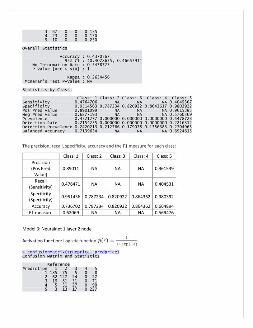
3 67 0 0 0 135 4 23 0 0 0 130 5 10 0 0 0 250 Overall Statistics Accuracy : 0.4370567 95% CI : (0.4078635, 0.4665791) No Information Rate : 0.5478723 P-Value [Acc > NIR] : 1 Kappa : 0.2634456 Mcnemar's Test P-Value : NA Statistics by Class: Class: 1 Class: 2 Class: 3 Class: 4 Class: 5 Sensitivity 0.4764706 NA NA NA 0.4045307 Specificity 0.9514563 0.787234 0.820922 0.8643617 0.9803922 Pos Pred Value 0.8901099 NA NA NA 0.9615385 Neg Pred Value 0.6877193 NA NA NA 0.5760369 Prevalence 0.4521277 0.000000 0.000000 0.0000000 0.5478723 Detection Rate 0.2154255 0.000000 0.000000 0.0000000 0.2216312 Detection Prevalence 0.2420213 0.212766 0.179078 0.1356383 0.2304965 Balanced Accuracy 0.7139634 NA NA NA 0.6924615
The precision, recall, specificity, accuracy and the F1 measure for each class:
Class: 1 Class: 2 Class: 3 Class: 4 Class: 5
Precision (Pos Pred
Value) 0.89011 NA NA NA 0.961539
Recall (Sensitivity)
0.476471 NA NA NA 0.404531
Specificity (Specificity)
0.951456 0.787234 0.820922 0.864362 0.980392
Accuracy 0.736702 0.787234 0.820922 0.864362 0.664894
F1 measure 0.62069 NA NA NA 0.569476
Model 3: Neuralnet 1 layer 2 node
Activation function: Logistic function ∅(ε) =1
1+exp(−𝜀)
> confusionMatrix(trueprice, predprice) Confusion Matrix and Statistics Reference Prediction 1 2 3 4 5 1 185 75 5 0 8 2 62 127 24 0 27 3 19 81 31 0 71 4 5 31 27 0 90 5 3 13 17 0 227

Overall Statistics Accuracy : 0.5053191 95% CI : (0.4757175, 0.534893) No Information Rate : 0.375 P-Value [Acc > NIR] : < 0.00000000000000022204 Kappa : 0.3630047 Mcnemar's Test P-Value : < 0.00000000000000022204 Statistics by Class: Class: 1 Class: 2 Class: 3 Class: 4 Class: 5 Sensitivity 0.6751825 0.3883792 0.29807692 NA 0.5366430 Specificity 0.8969555 0.8589263 0.83300781 0.8643617 0.9531915 Pos Pred Value 0.6776557 0.5291667 0.15346535 NA 0.8730769 Neg Pred Value 0.8959064 0.7747748 0.92116631 NA 0.7741935 Prevalence 0.2429078 0.2898936 0.09219858 0.0000000 0.3750000 Detection Rate 0.1640071 0.1125887 0.02748227 0.0000000 0.2012411 Detection Prevalence 0.2420213 0.2127660 0.17907801 0.1356383 0.2304965 Balanced Accuracy 0.7860690 0.6236528 0.56554237 NA 0.7449173
The precision, recall, specificity, accuracy and the F1 measure for each class:
Class: 1 Class: 2 Class: 3 Class: 4 Class: 5
Precision (Pos Pred
Value) 0.677656 0.529167 0.153465 NA 0.873077
Recall (Sensitivity)
0.675183 0.388379 0.298077 NA 0.536643
Specificity (Specificity)
0.896956 0.858926 0.833008 0.864362 0.953192
Accuracy 0.843085 0.722518 0.783688 0.864362 0.796986
F1 measure 0.676417 0.447972 0.202614 NA 0.664714
Model 4: Neuralnet 2 layer c=(3,2)
Activation function: Logistic function ∅(ε) =1
1+exp(−𝜀)
> confusionMatrix(trueprice, predprice) Confusion Matrix and Statistics Reference Prediction 1 2 3 4 5 1 195 69 1 0 8 2 66 141 6 0 27 3 21 108 13 0 60 4 6 50 7 0 90 5 2 32 4 0 222 Overall Statistics Accuracy : 0.5062057 95% CI : (0.4766023, 0.5357766)

No Information Rate : 0.3608156 P-Value [Acc > NIR] : < 0.00000000000000022204 Kappa : 0.3622215 Mcnemar's Test P-Value : < 0.00000000000000022204 Statistics by Class: Class: 1 Class: 2 Class: 3 Class: 4 Class: 5 Sensitivity 0.6724138 0.3525000 0.41935484 NA 0.5454545 Specificity 0.9069212 0.8640110 0.82771194 0.8643617 0.9472954 Pos Pred Value 0.7142857 0.5875000 0.06435644 NA 0.8538462 Neg Pred Value 0.8888889 0.7083333 0.98056156 NA 0.7868664 Prevalence 0.2570922 0.3546099 0.02748227 0.0000000 0.3608156 Detection Rate 0.1728723 0.1250000 0.01152482 0.0000000 0.1968085 Detection Prevalence 0.2420213 0.2127660 0.17907801 0.1356383 0.2304965 Balanced Accuracy 0.7896675 0.6082555 0.62353339 NA 0.7463750
The precision, recall, specificity, accuracy and the F1 measure for each class:
Class: 1 Class: 2 Class: 3 Class: 4 Class: 5
Precision (Pos Pred
Value) 0.714286 0.5875 0.064356 NA 0.853846
Recall (Sensitivity)
0.672414 0.3525 0.419355 NA 0.545455
Specificity (Specificity)
0.906921 0.864011 0.827712 0.864362 0.947295
Accuracy 0.846631 0.682624 0.816489 0.864362 0.802305
F1 measure 0.692718 0.440625 0.111588 NA 0.665667
Model 5: Neuralnet 2 layer c=(2,2)
Activation function: Logistic function ∅(ε) =1
1+exp(−𝜀)
> confusionMatrix(trueprice, predprice) Confusion Matrix and Statistics Reference Prediction 1 2 3 4 5 1 191 64 11 0 7 2 64 120 33 0 23 3 20 61 57 0 64 4 6 19 38 0 90 5 4 7 31 0 218 Overall Statistics Accuracy : 0.5195035 95% CI : (0.4898853, 0.5490198) No Information Rate : 0.356383 P-Value [Acc > NIR] : < 0.00000000000000022204 Kappa : 0.3828717

Mcnemar's Test P-Value : < 0.00000000000000022204 Statistics by Class: Class: 1 Class: 2 Class: 3 Class: 4 Class: 5 Sensitivity 0.6701754 0.4428044 0.33529412 NA 0.5422886 Specificity 0.9027284 0.8599767 0.84864301 0.8643617 0.9421488 Pos Pred Value 0.6996337 0.5000000 0.28217822 NA 0.8384615 Neg Pred Value 0.8900585 0.8299550 0.87796976 NA 0.7880184 Prevalence 0.2526596 0.2402482 0.15070922 0.0000000 0.3563830 Detection Rate 0.1693262 0.1063830 0.05053191 0.0000000 0.1932624 Detection Prevalence 0.2420213 0.2127660 0.17907801 0.1356383 0.2304965 Balanced Accuracy 0.7864519 0.6513905 0.59196856 NA 0.7422187
The precision, recall, specificity, accuracy and the F1 measure for each class:
Class: 1 Class: 2 Class: 3 Class: 4 Class: 5
Precision (Pos Pred
Value) 0.699634 0.5 0.282178 NA 0.838462
Recall (Sensitivity)
0.670175 0.442804 0.335294 NA 0.542289
Specificity (Specificity)
0.902728 0.859977 0.848643 0.864362 0.942149
Accuracy 0.843972 0.759752 0.771277 0.864362 0.799645
F1 measure 0.684588 0.469667 0.306452 NA 0.65861
Model 6: Neuralnet 2 layer c=(5,3)
Activation function: Logistic function ∅(ε) =1
1+exp(−𝜀)
> confusionMatrix(trueprice, predprice) Confusion Matrix and Statistics Reference Prediction 1 2 3 4 5 1 147 105 18 0 3 2 39 140 51 0 10 3 11 66 88 0 37 4 4 18 58 0 73 5 3 11 45 0 201 Overall Statistics Accuracy : 0.5106383 95% CI : (0.4810277, 0.5401933) No Information Rate : 0.3014184 P-Value [Acc > NIR] : < 0.00000000000000022204 Kappa : 0.3763037 Mcnemar's Test P-Value : < 0.00000000000000022204 Statistics by Class:

Class: 1 Class: 2 Class: 3 Class: 4 Class: 5 Sensitivity 0.7205882 0.4117647 0.33846154 NA 0.6203704 Specificity 0.8636364 0.8730964 0.86866359 0.8643617 0.9266169 Pos Pred Value 0.5384615 0.5833333 0.43564356 NA 0.7730769 Neg Pred Value 0.9333333 0.7747748 0.81425486 NA 0.8582949 Prevalence 0.1808511 0.3014184 0.23049645 0.0000000 0.2872340 Detection Rate 0.1303191 0.1241135 0.07801418 0.0000000 0.1781915 Detection Prevalence 0.2420213 0.2127660 0.17907801 0.1356383 0.2304965 Balanced Accuracy 0.7921123 0.6424306 0.60356257 NA 0.7734936
The precision, recall, specificity, accuracy and the F1 measure for each class:
Class: 1 Class: 2 Class: 3 Class: 4 Class: 5
Precision (Pos Pred
Value) 0.538462 0.583333 0.435644 NA 0.773077
Recall (Sensitivity)
0.720588 0.411765 0.338462 NA 0.62037
Specificity (Specificity)
0.863636 0.873096 0.868664 0.864362 0.926617
Accuracy 0.837766 0.734043 0.746454 0.864362 0.838653
F1 measure 0.616352 0.482759 0.380952 NA 0.688356
Model 7: Neuralnet 1 layer c=2
Activation function: Tanh function f(z) = tanh(z) =𝑒𝑧−𝑒𝑧
𝑒𝑧+𝑒𝑧
> confusionMatrix(trueprice, predprice) Confusion Matrix and Statistics Reference Prediction 1 2 3 4 5 1 243 0 0 0 30 2 167 0 0 0 73 3 67 0 0 0 135 4 23 0 0 0 130 5 10 0 0 0 250 Overall Statistics Accuracy : 0.4370567 95% CI : (0.4078635, 0.4665791) No Information Rate : 0.5478723 P-Value [Acc > NIR] : 1 Kappa : 0.2634456 Mcnemar's Test P-Value : NA Statistics by Class: Class: 1 Class: 2 Class: 3 Class: 4 Class: 5 Sensitivity 0.4764706 NA NA NA 0.4045307 Specificity 0.9514563 0.787234 0.820922 0.8643617 0.9803922 Pos Pred Value 0.8901099 NA NA NA 0.9615385

Neg Pred Value 0.6877193 NA NA NA 0.5760369 Prevalence 0.4521277 0.000000 0.000000 0.0000000 0.5478723 Detection Rate 0.2154255 0.000000 0.000000 0.0000000 0.2216312 Detection Prevalence 0.2420213 0.212766 0.179078 0.1356383 0.2304965 Balanced Accuracy 0.7139634 NA NA NA 0.6924615
The precision, recall, specificity, accuracy and the F1 measure for each class:
Class: 1 Class: 2 Class: 3 Class: 4 Class: 5
Precision (Pos Pred
Value) 0.89011 NA NA NA 0.961539
Recall (Sensitivity)
0.476471 NA NA NA 0.404531
Specificity (Specificity)
0.951456 0.787234 0.820922 0.864362 0.980392
Accuracy 0.736702 0.787234 0.820922 0.864362 0.664894
F1 measure 0.62069 NA NA NA 0.569476
Plot of best model:
Layer 2, c= (2, 2), activation function: logistic
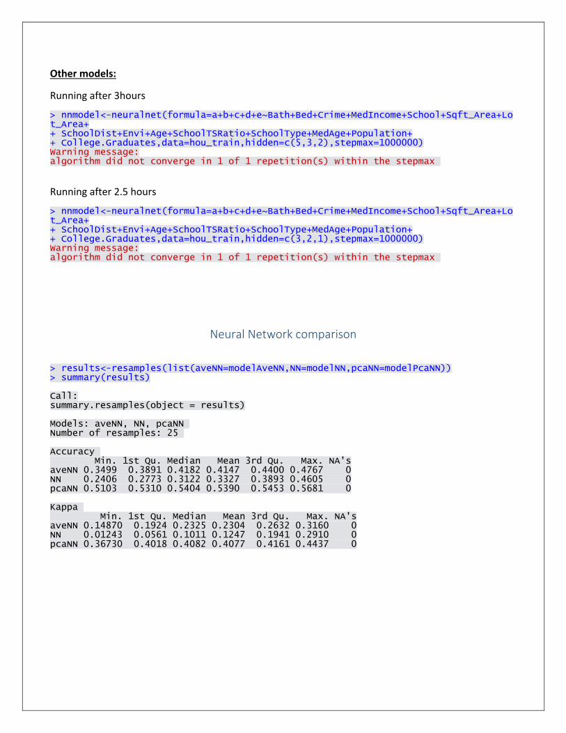
Other models:
Running after 3hours
> nnmodel<-neuralnet(formula=a+b+c+d+e~Bath+Bed+Crime+MedIncome+School+Sqft_Area+Lot_Area+ + SchoolDist+Envi+Age+SchoolTSRatio+SchoolType+MedAge+Population+ + College.Graduates,data=hou_train,hidden=c(5,3,2),stepmax=1000000) Warning message: algorithm did not converge in 1 of 1 repetition(s) within the stepmax
Running after 2.5 hours
> nnmodel<-neuralnet(formula=a+b+c+d+e~Bath+Bed+Crime+MedIncome+School+Sqft_Area+Lot_Area+ + SchoolDist+Envi+Age+SchoolTSRatio+SchoolType+MedAge+Population+ + College.Graduates,data=hou_train,hidden=c(3,2,1),stepmax=1000000) Warning message: algorithm did not converge in 1 of 1 repetition(s) within the stepmax
Neural Network comparison
> results<-resamples(list(aveNN=modelAveNN,NN=modelNN,pcaNN=modelPcaNN)) > summary(results) Call: summary.resamples(object = results) Models: aveNN, NN, pcaNN Number of resamples: 25 Accuracy Min. 1st Qu. Median Mean 3rd Qu. Max. NA's aveNN 0.3499 0.3891 0.4182 0.4147 0.4400 0.4767 0 NN 0.2406 0.2773 0.3122 0.3327 0.3893 0.4605 0 pcaNN 0.5103 0.5310 0.5404 0.5390 0.5453 0.5681 0 Kappa Min. 1st Qu. Median Mean 3rd Qu. Max. NA's aveNN 0.14870 0.1924 0.2325 0.2304 0.2632 0.3160 0 NN 0.01243 0.0561 0.1011 0.1247 0.1941 0.2910 0 pcaNN 0.36730 0.4018 0.4082 0.4077 0.4161 0.4437 0

Question 3: Clustering
We ran the following clustering methods:
• K-means
• K-Medoids
• Hierarchical
• Density‐based
• Mixture model
K-Means Clustering Step 1: Divide Price Range into 5 Categories.
Step 2: Make sure all data values are numeric
K-Means cannot handle non-numeric or categorical values
Step 3: Standardize all data
Step 4: Remove the response variable (Price)
Step 3: Run K-Means Analysis for cluster numbers 3 and 5.

K-Means Clustering: (5 clusters)
Number of clusters and number of elements per cluster:
> kmeans.result # Display values K-means clustering with 5 clusters of sizes 23, 56, 1093, 1957, 295
Means of Clusters
Cluster means: Latitude Longitude Bath Bed Postal Crime MedIncome School Sqft_Area Lot_Area SchoolDist 1 47.70171 -122.3378 1.760870 4.913043 98133.74 0.3142468 -0.195018414 1.695652 1277.6957 78408.000 0.6740977 2 47.72415 -122.3434 1.473214 5.928571 98132.04 0.2129911 -0.752875977 1.625000 962.1964 208123.457 0.3063229 3 47.61045 -122.3258 1.729414 2.814273 98120.46 -0.1073124 0.034888745 3.093321 1822.3898 4880.782 0.4662398 4 47.60653 -122.3287 2.014262 2.622892 98125.53 0.2596665 0.007965796 2.856413 1807.8401 5512.804 0.4933124 5 47.64879 -122.3206 1.930000 3.498305 98128.99 0.2108353 -0.247995762 2.911864 1887.0475 13064.866 0.5324636 Built_Year Price_Sqft Envi Age SchoolType SchoolTSRatio SchoolRating MedAge Population College.Graduates 1 1973.217 221.7826 2.739130 1789.478 7.695652 17.39130 4.956522 39.24348 0.6572639 41.43130 2 1982.268 194.5714 0.750000 1075.875 8.000000 16.78571 4.107143 38.84464 0.9597902 37.04250 3 1917.283 287.7402 5.591949 9434.624 7.365965 18.25892 6.160110 36.75215 -0.1388636 43.47220 4 1966.412 250.1579 3.170669 2900.260 7.120082 17.51865 4.980072 37.95968 -0.1509776 37.43829 5 1964.369 234.6983 2.620339 3159.983 6.386441 16.76610 4.528814 38.38610 0.2326572 38.40654 Rank 1 -0.09823492 2 -0.02066822 3 -0.02152379 4 0.35099686 5 0.15977362
Within cluster sum of squares
Within cluster sum of squares by cluster: [1] 5887803872 27215557012 7071976251 16113352985 9513281345 (between_SS / total_SS = 97.3 %)
97.3% is the measure of the total variance that is explained by the clustering.
Check Clustering against actual price
> # Check clustering against actual Price > table(hou$Price,kmeans.result$cluster) 1 2 3 4 5 100,000 to <200,000 14 46 84 116 68 200,000 to <400,000 3 9 313 914 90 400,000 to <600,000 2 1 358 589 59

600,000 to <800,000 2 0 228 236 45 800,000 to 1,000,000 2 0 110 102 33
The clusters are not too good a representation of our data. Ideally, each cluster should be well
separated from the others and there should be minimum overlap. However, 3, 4, 5 clusters show high
overlapping. The first two (second cluster is better represented) are still comparable ok and they
mostly are the ‘100,000 to <200,000’ range with slight overlapping with other ranges.
Number of Elements in each cluster:
> kmeans.result$size [1] 23 56 1093 1957 295
For intuitive purpose, we picked ‘Postal’ and ‘College.Graduates’ and plotted it to observe the cluster
Looking at the model although the clusters obtained are not too good at least they show some
separation (better than the various other runs we tried). Some clusters are well separated while some
are close. This could also be the case as we considered 5 clusters.

Multiple Runs: (4 runs results displayed) (They are grouped as below for better viewing of results)
Number of clusters and number of elements per cluster:
Run1: > kmeans.result # Display values K-means clustering with 5 clusters of sizes 23, 1957, 1093, 295, 56
Run2: > kmeans.result # Display values K-means clustering with 5 clusters of sizes 1957, 56, 295, 23, 1093
Run3: > kmeans.result # Display values K-means clustering with 5 clusters of sizes 295, 23, 1093, 1957, 56
Run4: > kmeans.result # Display values K-means clustering with 5 clusters of sizes 1957, 295, 23, 1093, 56
Means of Clusters
Run1: Cluster means: Latitude Longitude Bath Bed Postal Crime MedIncome School Sqft_Area Lot_Area SchoolDist Built_Year 1 47.70171 -122.3378 1.760870 4.913043 98133.74 0.3142468 -0.195018414 1.695652 1277.6957 78408.000 0.6740977 1973.217 2 47.60653 -122.3287 2.014262 2.622892 98125.53 0.2596665 0.007965796 2.856413 1807.8401 5512.804 0.4933124 1966.412 3 47.61045 -122.3258 1.729414 2.814273 98120.46 -0.1073124 0.034888745 3.093321 1822.3898 4880.782 0.4662398 1917.283 4 47.64879 -122.3206 1.930000 3.498305 98128.99 0.2108353 -0.247995762 2.911864 1887.0475 13064.866 0.5324636 1964.369 5 47.72415 -122.3434 1.473214 5.928571 98132.04 0.2129911 -0.752875977 1.625000 962.1964 208123.457 0.3063229 1982.268 Price_Sqft Envi Age SchoolType SchoolTSRatio SchoolRating MedAge Population College.Graduates Rank 1 221.7826 2.739130 1789.478 7.695652 17.39130 4.956522 39.24348 0.6572639 41.43130 -0.09823492 2 250.1579 3.170669 2900.260 7.120082 17.51865 4.980072 37.95968 -0.1509776 37.43829 0.35099686 3 287.7402 5.591949 9434.624 7.365965 18.25892 6.160110 36.75215 -0.1388636 43.47220 -0.02152379 4 234.6983 2.620339 3159.983 6.386441 16.76610 4.528814 38.38610 0.2326572 38.40654 0.15977362 5 194.5714 0.750000 1075.875 8.000000 16.78571 4.107143 38.84464 0.9597902 37.04250 -0.02066822
Run2: Cluster means: Latitude Longitude Bath Bed Postal Crime MedIncome School Sqft_Area Lot_Area

1 47.60653 -122.3287 2.014262 2.622892 98125.53 0.2596665 0.007965796 2.856413 1807.8401 5512.804 2 47.72415 -122.3434 1.473214 5.928571 98132.04 0.2129911 -0.752875977 1.625000 962.1964 208123.457 3 47.64879 -122.3206 1.930000 3.498305 98128.99 0.2108353 -0.247995762 2.911864 1887.0475 13064.866 4 47.70171 -122.3378 1.760870 4.913043 98133.74 0.3142468 -0.195018414 1.695652 1277.6957 78408.000 5 47.61045 -122.3258 1.729414 2.814273 98120.46 -0.1073124 0.034888745 3.093321 1822.3898 4880.782 SchoolDist Built_Year Price_Sqft Envi Age SchoolType SchoolTSRatio SchoolRating MedAge 1 0.4933124 1966.412 250.1579 3.170669 2900.260 7.120082 17.51865 4.980072 37.95968 2 0.3063229 1982.268 194.5714 0.750000 1075.875 8.000000 16.78571 4.107143 38.84464 3 0.5324636 1964.369 234.6983 2.620339 3159.983 6.386441 16.76610 4.528814 38.38610 4 0.6740977 1973.217 221.7826 2.739130 1789.478 7.695652 17.39130 4.956522 39.24348 5 0.4662398 1917.283 287.7402 5.591949 9434.624 7.365965 18.25892 6.160110 36.75215 Population College.Graduates Rank 1 -0.1509776 37.43829 0.35099686 2 0.9597902 37.04250 -0.02066822 3 0.2326572 38.40654 0.15977362 4 0.6572639 41.43130 -0.09823492 5 -0.1388636 43.47220 -0.02152379
Run3: Cluster means: Latitude Longitude Bath Bed Postal Crime MedIncome School Sqft_Area 1 47.64879 -122.3206 1.930000 3.498305 98128.99 0.2108353 -0.247995762 2.911864 1887.0475 2 47.70171 -122.3378 1.760870 4.913043 98133.74 0.3142468 -0.195018414 1.695652 1277.6957 3 47.61045 -122.3258 1.729414 2.814273 98120.46 -0.1073124 0.034888745 3.093321 1822.3898 4 47.60653 -122.3287 2.014262 2.622892 98125.53 0.2596665 0.007965796 2.856413 1807.8401 5 47.72415 -122.3434 1.473214 5.928571 98132.04 0.2129911 -0.752875977 1.625000 962.1964 Lot_Area SchoolDist Built_Year Price_Sqft Envi Age SchoolType SchoolTSRatio 1 13064.866 0.5324636 1964.369 234.6983 2.620339 3159.983 6.386441 16.76610 2 78408.000 0.6740977 1973.217 221.7826 2.739130 1789.478 7.695652 17.39130 3 4880.782 0.4662398 1917.283 287.7402 5.591949 9434.624 7.365965 18.25892 4 5512.804 0.4933124 1966.412 250.1579 3.170669 2900.260 7.120082 17.51865 5 208123.457 0.3063229 1982.268 194.5714 0.750000 1075.875 8.000000 16.78571 SchoolRating MedAge Population College.Graduates Rank 1 4.528814 38.38610 0.2326572 38.40654 0.15977362 2 4.956522 39.24348 0.6572639 41.43130 -0.09823492 3 6.160110 36.75215 -0.1388636 43.47220 -0.02152379 4 4.980072 37.95968 -0.1509776 37.43829 0.35099686 5 4.107143 38.84464 0.9597902 37.04250 -0.02066822
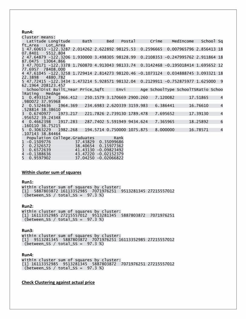
Run4: Cluster means: Latitude Longitude Bath Bed Postal Crime MedIncome School Sqft_Area Lot_Area 1 47.60653 -122.3287 2.014262 2.622892 98125.53 0.2596665 0.007965796 2.856413 1807.8401 5512.804 2 47.64879 -122.3206 1.930000 3.498305 98128.99 0.2108353 -0.247995762 2.911864 1887.0475 13064.866 3 47.70171 -122.3378 1.760870 4.913043 98133.74 0.3142468 -0.195018414 1.695652 1277.6957 78408.000 4 47.61045 -122.3258 1.729414 2.814273 98120.46 -0.1073124 0.034888745 3.093321 1822.3898 4880.782 5 47.72415 -122.3434 1.473214 5.928571 98132.04 0.2129911 -0.752875977 1.625000 962.1964 208123.457 SchoolDist Built_Year Price_Sqft Envi Age SchoolType SchoolTSRatio SchoolRating MedAge 1 0.4933124 1966.412 250.1579 3.170669 2900.260 7.120082 17.51865 4.980072 37.95968 2 0.5324636 1964.369 234.6983 2.620339 3159.983 6.386441 16.76610 4.528814 38.38610 3 0.6740977 1973.217 221.7826 2.739130 1789.478 7.695652 17.39130 4.956522 39.24348 4 0.4662398 1917.283 287.7402 5.591949 9434.624 7.365965 18.25892 6.160110 36.75215 5 0.3063229 1982.268 194.5714 0.750000 1075.875 8.000000 16.78571 4.107143 38.84464 Population College.Graduates Rank 1 -0.1509776 37.43829 0.35099686 2 0.2326572 38.40654 0.15977362 3 0.6572639 41.43130 -0.09823492 4 -0.1388636 43.47220 -0.02152379 5 0.9597902 37.04250 -0.02066822
Within cluster sum of squares
Run1: Within cluster sum of squares by cluster: [1] 5887803872 16113352985 7071976251 9513281345 27215557012 (between_SS / total_SS = 97.3 %)
Run2: Within cluster sum of squares by cluster: [1] 16113352985 27215557012 9513281345 5887803872 7071976251 (between_SS / total_SS = 97.3 %)
Run3: Within cluster sum of squares by cluster: [1] 9513281345 5887803872 7071976251 16113352985 27215557012 (between_SS / total_SS = 97.3 %)
Run4: Within cluster sum of squares by cluster: [1] 16113352985 9513281345 5887803872 7071976251 27215557012 (between_SS / total_SS = 97.3 %)
Check Clustering against actual price

Run1: > # Check clustering against actual Price > table(hou$Price,kmeans.result$cluster) 1 2 3 4 5 100,000 to <200,000 14 116 84 68 46 200,000 to <400,000 3 914 313 90 9 400,000 to <600,000 2 589 358 59 1 600,000 to <800,000 2 236 228 45 0 800,000 to 1,000,000 2 102 110 33 0
Run2: > table(hou$Price,kmeans.result$cluster) 1 2 3 4 5 100,000 to <200,000 116 46 68 14 84 200,000 to <400,000 914 9 90 3 313 400,000 to <600,000 589 1 59 2 358 600,000 to <800,000 236 0 45 2 228 800,000 to 1,000,000 102 0 33 2 110
Run3: > table(hou$Price,kmeans.result$cluster) 1 2 3 4 5 100,000 to <200,000 68 14 84 116 46 200,000 to <400,000 90 3 313 914 9 400,000 to <600,000 59 2 358 589 1 600,000 to <800,000 45 2 228 236 0 800,000 to 1,000,000 33 2 110 102 0
Run4: > table(hou$Price,kmeans.result$cluster) 1 2 3 4 5 100,000 to <200,000 116 68 14 84 46 200,000 to <400,000 914 90 3 313 9 400,000 to <600,000 589 59 2 358 1 600,000 to <800,000 236 45 2 228 0 800,000 to 1,000,000 102 33 2 110 0
Number of Elements in each cluster:
Run1: > kmeans.result$size [1] 23 1957 1093 295 56
Run2: > kmeans.result$size [1] 1957 56 295 23 1093
Run3: > kmeans.result$size [1] 295 23 1093 1957 56

Run4: > kmeans.result$size [1] 1957 295 23 1093 56
For intuitive purpose, we picked ‘Postal’ and ‘College.Graduates’ and plotted it to observe the cluster
Run1:
Run2:

Run3:
Run4:
It can be observed from the results of the multiple runs that the behavior of clusters doesn’t change.
It’s just the values of one cluster are represented by another cluster. Even the graph and overall
variance represented by the clusters are the same.

K-Means Clustering: (3 clusters)
Number of clusters and number of elements per cluster:
> kmeans.result # Display values K-means clustering with 3 clusters of sizes 1152, 2215, 57
Means of Clusters
Cluster means: Latitude Longitude Bath Bed Postal Crime MedIncome 1 47.61064 -122.3262 1.716797 2.831597 98120.53 -0.08768001 0.04340377 2 47.61291 -122.3276 2.015016 2.747178 98126.18 0.25301048 -0.03399338 3 47.72343 -122.3420 1.464912 5.947368 98131.74 0.22483636 -0.71558911 School Sqft_Area Lot_Area SchoolDist Built_Year Price_Sqft Envi 1 3.050347 1813.5061 4919.463 0.4680265 1918.231 287.5877 5.532118 2 2.868623 1817.6239 7223.020 0.5000488 1967.021 246.9201 3.057336 3 1.614035 957.3333 206482.042 0.3153170 1982.175 194.0877 0.877193 Age SchoolType SchoolTSRatio SchoolRating MedAge Population 1 9269.172 7.368056 18.27344 6.171875 36.80260 -0.14383482 2 2836.005 7.020316 17.38962 4.879910 38.03589 -0.08987959 3 1081.018 8.000000 16.80702 4.210526 38.82281 0.96559855 College.Graduates Rank 1 43.28285 -0.005963353 2 37.53440 0.323287360 3 37.51842 -0.037192464
Within cluster sum of squares
Within cluster sum of squares by cluster: [1] 8814471005 150456786996 35815743491 (between_SS / total_SS = 92.1 %)
92.1% is the measure of the total variance that is explained by the clustering. It decreased from the
above case where it was 97.3%.
Check Clustering against actual price
> table(hou$Price, kmeans.result$cluster) 1 2 3 >600,000 350 408 0 100,000 to <300,000 237 627 55 300,000 to <600,000 565 1180 2
The clusters are not too good a representation of our data. Ideally, each cluster should be well
separated from the others and there should be minimum overlap. However, 1, 2 clusters show high
overlapping. The third cluster is comparably ok and they mostly are the ‘100,000 to <300,000’ range
with slight overlapping with other ranges.
Number of Elements in each cluster: > kmeans.result$size [1] 1152 2215 57

For intuitive purpose, we picked ‘Postal’ and ‘College.Graduates’ and plotted it to observe the cluster
Looking at the model although the clusters obtained are not too good at least they show some separation
(better than the various other runs we tried)
Multiple Runs: (4 runs results displayed) (They are grouped as below for better viewing of results)
Number of clusters and number of elements per cluster:
Run1: > kmeans.result # Display values K-means clustering with 3 clusters of sizes 2215, 57, 1152
Run2: > kmeans.result # Display values K-means clustering with 3 clusters of sizes 1152, 2215, 57
Run3: > kmeans.result # Display values K-means clustering with 3 clusters of sizes 57, 2215, 1152
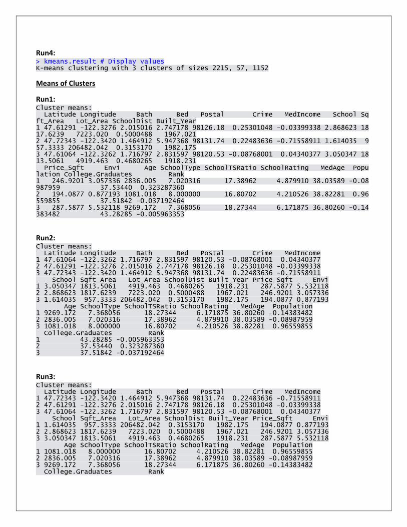
Run4: > kmeans.result # Display values K-means clustering with 3 clusters of sizes 2215, 57, 1152
Means of Clusters
Run1: Cluster means: Latitude Longitude Bath Bed Postal Crime MedIncome School Sqft_Area Lot_Area SchoolDist Built_Year 1 47.61291 -122.3276 2.015016 2.747178 98126.18 0.25301048 -0.03399338 2.868623 1817.6239 7223.020 0.5000488 1967.021 2 47.72343 -122.3420 1.464912 5.947368 98131.74 0.22483636 -0.71558911 1.614035 957.3333 206482.042 0.3153170 1982.175 3 47.61064 -122.3262 1.716797 2.831597 98120.53 -0.08768001 0.04340377 3.050347 1813.5061 4919.463 0.4680265 1918.231 Price_Sqft Envi Age SchoolType SchoolTSRatio SchoolRating MedAge Population College.Graduates Rank 1 246.9201 3.057336 2836.005 7.020316 17.38962 4.879910 38.03589 -0.08987959 37.53440 0.323287360 2 194.0877 0.877193 1081.018 8.000000 16.80702 4.210526 38.82281 0.96559855 37.51842 -0.037192464 3 287.5877 5.532118 9269.172 7.368056 18.27344 6.171875 36.80260 -0.14383482 43.28285 -0.005963353
Run2: Cluster means: Latitude Longitude Bath Bed Postal Crime MedIncome 1 47.61064 -122.3262 1.716797 2.831597 98120.53 -0.08768001 0.04340377 2 47.61291 -122.3276 2.015016 2.747178 98126.18 0.25301048 -0.03399338 3 47.72343 -122.3420 1.464912 5.947368 98131.74 0.22483636 -0.71558911 School Sqft_Area Lot_Area SchoolDist Built_Year Price_Sqft Envi 1 3.050347 1813.5061 4919.463 0.4680265 1918.231 287.5877 5.532118 2 2.868623 1817.6239 7223.020 0.5000488 1967.021 246.9201 3.057336 3 1.614035 957.3333 206482.042 0.3153170 1982.175 194.0877 0.877193 Age SchoolType SchoolTSRatio SchoolRating MedAge Population 1 9269.172 7.368056 18.27344 6.171875 36.80260 -0.14383482 2 2836.005 7.020316 17.38962 4.879910 38.03589 -0.08987959 3 1081.018 8.000000 16.80702 4.210526 38.82281 0.96559855 College.Graduates Rank 1 43.28285 -0.005963353 2 37.53440 0.323287360 3 37.51842 -0.037192464
Run3: Cluster means: Latitude Longitude Bath Bed Postal Crime MedIncome 1 47.72343 -122.3420 1.464912 5.947368 98131.74 0.22483636 -0.71558911 2 47.61291 -122.3276 2.015016 2.747178 98126.18 0.25301048 -0.03399338 3 47.61064 -122.3262 1.716797 2.831597 98120.53 -0.08768001 0.04340377 School Sqft_Area Lot_Area SchoolDist Built_Year Price_Sqft Envi 1 1.614035 957.3333 206482.042 0.3153170 1982.175 194.0877 0.877193 2 2.868623 1817.6239 7223.020 0.5000488 1967.021 246.9201 3.057336 3 3.050347 1813.5061 4919.463 0.4680265 1918.231 287.5877 5.532118 Age SchoolType SchoolTSRatio SchoolRating MedAge Population 1 1081.018 8.000000 16.80702 4.210526 38.82281 0.96559855 2 2836.005 7.020316 17.38962 4.879910 38.03589 -0.08987959 3 9269.172 7.368056 18.27344 6.171875 36.80260 -0.14383482 College.Graduates Rank

1 37.51842 -0.037192464 2 37.53440 0.323287360 3 43.28285 -0.005963353
Run4: Cluster means: Latitude Longitude Bath Bed Postal Crime MedIncome 1 47.61291 -122.3276 2.015016 2.747178 98126.18 0.25301048 -0.03399338 2 47.72343 -122.3420 1.464912 5.947368 98131.74 0.22483636 -0.71558911 3 47.61064 -122.3262 1.716797 2.831597 98120.53 -0.08768001 0.04340377 School Sqft_Area Lot_Area SchoolDist Built_Year Price_Sqft Envi 1 2.868623 1817.6239 7223.020 0.5000488 1967.021 246.9201 3.057336 2 1.614035 957.3333 206482.042 0.3153170 1982.175 194.0877 0.877193 3 3.050347 1813.5061 4919.463 0.4680265 1918.231 287.5877 5.532118 Age SchoolType SchoolTSRatio SchoolRating MedAge Population 1 2836.005 7.020316 17.38962 4.879910 38.03589 -0.08987959 2 1081.018 8.000000 16.80702 4.210526 38.82281 0.96559855 3 9269.172 7.368056 18.27344 6.171875 36.80260 -0.14383482 College.Graduates Rank 1 37.53440 0.323287360 2 37.51842 -0.037192464 3 43.28285 -0.005963353
Within cluster sum of squares
Run1: Within cluster sum of squares by cluster: [1] 150456786996 35815743491 8814471005 (between_SS / total_SS = 92.1 %)
Run2: Within cluster sum of squares by cluster: [1] 8814471005 150456786996 35815743491 (between_SS / total_SS = 92.1 %)
Run3: Within cluster sum of squares by cluster: [1] 35815743491 150456786996 8814471005 (between_SS / total_SS = 92.1 %)
Run4: Within cluster sum of squares by cluster: [1] 150456786996 35815743491 8814471005 (between_SS / total_SS = 92.1 %)
Check Clustering against actual price
Run1: > table(hou$Price, kmeans.result$cluster) 1 2 3 >600,000 408 0 350 100,000 to <300,000 627 55 237 300,000 to <600,000 1180 2 565
Run2: > table(hou$Price, kmeans.result$cluster)

1 2 3 >600,000 350 408 0 100,000 to <300,000 237 627 55 300,000 to <600,000 565 1180 2
Run3: > table(hou$Price, kmeans.result$cluster) 1 2 3 >600,000 0 408 350 100,000 to <300,000 55 627 237 300,000 to <600,000 2 1180 565
Run4: > table(hou$Price, kmeans.result$cluster) 1 2 3 100,000 to <300,000 237 627 55 300,000 to <600,000 565 1180 2 600,000 to <900,000 307 356 0 900,000+ 43 52 0
Number of Elements in each cluster:
Run1: > kmeans.result$size [1] 2215 57 1152
Run2: > kmeans.result$size [1] 1152 2215 57
Run3: > kmeans.result$size [1] 57 2215 1152
Run4: > kmeans.result$size [1] 1152 2215 57

For intuitive purpose, we picked ‘Postal’ and ‘College.Graduates’ and plotted it to observe the cluster
Run1:
Run2:

Run3:
Run4:
Not much changes can be seen in multiple runs.

K-Means Clustering: (7 clusters)
Number of clusters and number of elements per cluster:
> kmeans.result # Display values K-means clustering with 7 clusters of sizes 56, 197, 23, 617, 1425, 882, 224
Means of Clusters
Cluster means: Latitude Longitude Bath Bed Postal Crime MedIncome School Sqft_Area Lot_Area SchoolDist Built_Year 1 47.72415 -122.3434 1.473214 5.928571 98132.04 0.2129911 -0.75287598 1.625000 962.1964 208123.457 0.3063229 1982.268 2 47.65550 -122.3195 1.861929 4.060914 98129.27 0.1745379 -0.30784309 3.050761 1757.0558 14516.050 0.5416982 1971.234 3 47.70171 -122.3378 1.760870 4.913043 98133.74 0.3142468 -0.19501841 1.695652 1277.6957 78408.000 0.6740977 1973.217 4 47.59899 -122.3264 2.719222 2.359806 98123.12 0.1244455 -0.20427870 2.865478 2032.1442 3940.180 0.4837208 1999.815 5 47.61158 -122.3296 1.708561 2.724912 98126.86 0.3187644 0.09633281 2.839298 1727.2021 6410.587 0.4988943 1951.245 6 47.61693 -122.3266 1.747449 2.764172 98119.75 -0.1943697 0.07344092 3.157596 1834.7687 4235.337 0.4522494 1916.693 7 47.58595 -122.3210 1.700893 2.964286 98123.02 0.2638358 -0.15535889 2.812500 1816.9286 8107.064 0.5228157 1920.004 Price_Sqft Envi Age SchoolType SchoolTSRatio SchoolRating MedAge Population College.Graduates Rank 1 194.5714 0.750000 1075.8750 8.000000 16.78571 4.107143 38.84464 0.9597902 37.04250 -0.02066822 2 231.6041 2.573604 2544.2995 5.939086 16.60914 4.517766 38.45482 0.2820359 38.59838 0.10188719 3 221.7826 2.739130 1789.4783 7.695652 17.39130 4.956522 39.24348 0.6572639 41.43130 -0.09823492 4 236.4878 3.685575 374.8752 7.183144 17.26094 4.764992 37.60227 -0.1173300 35.64921 0.44840083 5 255.3642 2.902456 4048.5656 7.110877 17.60281 5.061053 38.15347 -0.1526263 38.27999 0.30089620 6 297.9819 6.035147 9549.0760 7.373016 18.47392 6.503401 36.48379 -0.1390476 45.52034 -0.14322954 7 245.7232 3.794643 8910.8527 7.281250 17.35268 4.629464 37.75670 -0.0966216 34.88580 0.49698598
Within cluster sum of squares
Within cluster sum of squares by cluster: [1] 27215557012 7344672718 5887803872 3127837088 6172138242 4061335623 1390049151 (between_SS / total_SS = 97.8 %)
97.8% is the measure of the total variance that is explained by the clustering.
Check Clustering against actual price
> # Check clustering against actual Price > table(hou$Price, kmeans.result$cluster)

1 2 3 4 5 6 7 <200,000 46 63 14 23 97 55 30 <300,000 8 36 3 92 315 95 42 <400,000 1 25 0 165 368 133 46 <500,000 1 14 2 117 268 161 38 <600,000 0 7 0 85 156 133 27 <700,000 0 17 1 53 103 128 11 700,000 to 1,000,000 0 35 3 82 118 177 30
The clusters are not too good a representation of our data. Ideally, each cluster should be well separated from
the others and there should be minimum overlap. However, 4, 5, 6, 7 clusters show high overlapping. The first
and third cluster is comparably ok and they mostly are the ‘100,000 to <200,000’ range with slight overlapping
with other ranges.
Number of Elements in each cluster:
> kmeans.result$size [1] 56 197 23 617 1425 882 224
For intuitive purpose, we picked ‘Postal’ and ‘College.Graduates’ and plotted it to observe the cluster

Even though 7 clusters give higher variance estimation, the number of cluster overlapping is high thus
we prefer 5 clusters over this.
Multiple Runs: (4 runs results displayed) (They are grouped as below for better viewing of results)
Number of clusters and number of elements per cluster:
Run1 > kmeans.result # Display values K-means clustering with 7 clusters of sizes 56, 197, 23, 617, 1425, 882, 224
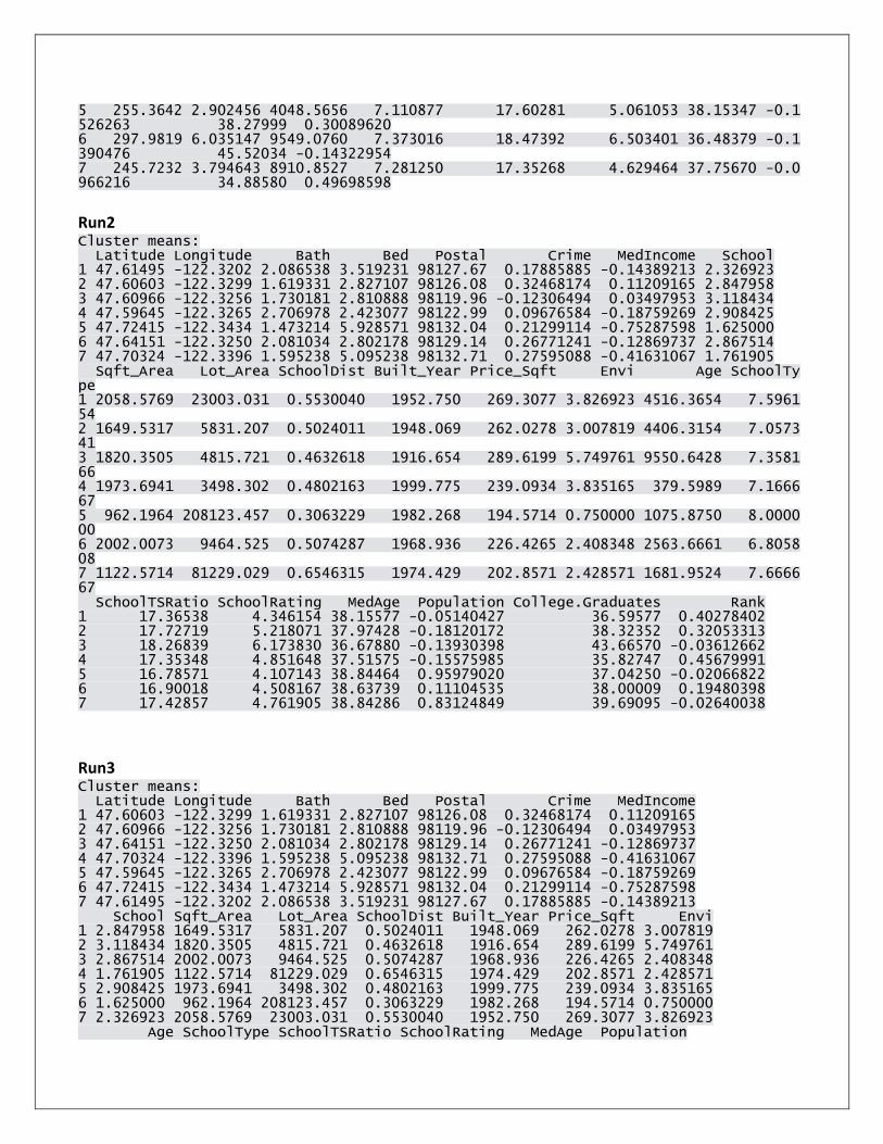
Run2 > kmeans.result # Display values K-means clustering with 7 clusters of sizes 52, 1151, 1047, 546, 56, 551, 21
Run3 > kmeans.result # Display values K-means clustering with 7 clusters of sizes 1151, 1047, 551, 21, 546, 56, 52
Run4 > kmeans.result # Display values K-means clustering with 7 clusters of sizes 729 1379 533 56 499 23 205
Means of Clusters
Run1 Cluster means: Latitude Longitude Bath Bed Postal Crime MedIncome School Sqft_Area Lot_Area SchoolDist Built_Year 1 47.72415 -122.3434 1.473214 5.928571 98132.04 0.2129911 -0.75287598 1.625000 962.1964 208123.457 0.3063229 1982.268 2 47.65550 -122.3195 1.861929 4.060914 98129.27 0.1745379 -0.30784309 3.050761 1757.0558 14516.050 0.5416982 1971.234 3 47.70171 -122.3378 1.760870 4.913043 98133.74 0.3142468 -0.19501841 1.695652 1277.6957 78408.000 0.6740977 1973.217 4 47.59899 -122.3264 2.719222 2.359806 98123.12 0.1244455 -0.20427870 2.865478 2032.1442 3940.180 0.4837208 1999.815 5 47.61158 -122.3296 1.708561 2.724912 98126.86 0.3187644 0.09633281 2.839298 1727.2021 6410.587 0.4988943 1951.245 6 47.61693 -122.3266 1.747449 2.764172 98119.75 -0.1943697 0.07344092 3.157596 1834.7687 4235.337 0.4522494 1916.693 7 47.58595 -122.3210 1.700893 2.964286 98123.02 0.2638358 -0.15535889 2.812500 1816.9286 8107.064 0.5228157 1920.004 Price_Sqft Envi Age SchoolType SchoolTSRatio SchoolRating MedAge Population College.Graduates Rank 1 194.5714 0.750000 1075.8750 8.000000 16.78571 4.107143 38.84464 0.9597902 37.04250 -0.02066822 2 231.6041 2.573604 2544.2995 5.939086 16.60914 4.517766 38.45482 0.2820359 38.59838 0.10188719 3 221.7826 2.739130 1789.4783 7.695652 17.39130 4.956522 39.24348 0.6572639 41.43130 -0.09823492 4 236.4878 3.685575 374.8752 7.183144 17.26094 4.764992 37.60227 -0.1173300 35.64921 0.44840083
5 255.3642 2.902456 4048.5656 7.110877 17.60281 5.061053 38.15347 -0.1526263 38.27999 0.30089620 6 297.9819 6.035147 9549.0760 7.373016 18.47392 6.503401 36.48379 -0.1390476 45.52034 -0.14322954 7 245.7232 3.794643 8910.8527 7.281250 17.35268 4.629464 37.75670 -0.0966216 34.88580 0.49698598
Run2 Cluster means: Latitude Longitude Bath Bed Postal Crime MedIncome School 1 47.61495 -122.3202 2.086538 3.519231 98127.67 0.17885885 -0.14389213 2.326923 2 47.60603 -122.3299 1.619331 2.827107 98126.08 0.32468174 0.11209165 2.847958 3 47.60966 -122.3256 1.730181 2.810888 98119.96 -0.12306494 0.03497953 3.118434 4 47.59645 -122.3265 2.706978 2.423077 98122.99 0.09676584 -0.18759269 2.908425 5 47.72415 -122.3434 1.473214 5.928571 98132.04 0.21299114 -0.75287598 1.625000 6 47.64151 -122.3250 2.081034 2.802178 98129.14 0.26771241 -0.12869737 2.867514 7 47.70324 -122.3396 1.595238 5.095238 98132.71 0.27595088 -0.41631067 1.761905 Sqft_Area Lot_Area SchoolDist Built_Year Price_Sqft Envi Age SchoolType 1 2058.5769 23003.031 0.5530040 1952.750 269.3077 3.826923 4516.3654 7.596154 2 1649.5317 5831.207 0.5024011 1948.069 262.0278 3.007819 4406.3154 7.057341 3 1820.3505 4815.721 0.4632618 1916.654 289.6199 5.749761 9550.6428 7.358166 4 1973.6941 3498.302 0.4802163 1999.775 239.0934 3.835165 379.5989 7.166667 5 962.1964 208123.457 0.3063229 1982.268 194.5714 0.750000 1075.8750 8.000000 6 2002.0073 9464.525 0.5074287 1968.936 226.4265 2.408348 2563.6661 6.805808 7 1122.5714 81229.029 0.6546315 1974.429 202.8571 2.428571 1681.9524 7.666667 SchoolTSRatio SchoolRating MedAge Population College.Graduates Rank 1 17.36538 4.346154 38.15577 -0.05140427 36.59577 0.40278402 2 17.72719 5.218071 37.97428 -0.18120172 38.32352 0.32053313 3 18.26839 6.173830 36.67880 -0.13930398 43.66570 -0.03612662 4 17.35348 4.851648 37.51575 -0.15575985 35.82747 0.45679991 5 16.78571 4.107143 38.84464 0.95979020 37.04250 -0.02066822 6 16.90018 4.508167 38.63739 0.11104535 38.00009 0.19480398 7 17.42857 4.761905 38.84286 0.83124849 39.69095 -0.02640038
Run3 Cluster means: Latitude Longitude Bath Bed Postal Crime MedIncome 1 47.60603 -122.3299 1.619331 2.827107 98126.08 0.32468174 0.11209165 2 47.60966 -122.3256 1.730181 2.810888 98119.96 -0.12306494 0.03497953 3 47.64151 -122.3250 2.081034 2.802178 98129.14 0.26771241 -0.12869737 4 47.70324 -122.3396 1.595238 5.095238 98132.71 0.27595088 -0.41631067 5 47.59645 -122.3265 2.706978 2.423077 98122.99 0.09676584 -0.18759269 6 47.72415 -122.3434 1.473214 5.928571 98132.04 0.21299114 -0.75287598 7 47.61495 -122.3202 2.086538 3.519231 98127.67 0.17885885 -0.14389213 School Sqft_Area Lot_Area SchoolDist Built_Year Price_Sqft Envi 1 2.847958 1649.5317 5831.207 0.5024011 1948.069 262.0278 3.007819 2 3.118434 1820.3505 4815.721 0.4632618 1916.654 289.6199 5.749761 3 2.867514 2002.0073 9464.525 0.5074287 1968.936 226.4265 2.408348 4 1.761905 1122.5714 81229.029 0.6546315 1974.429 202.8571 2.428571 5 2.908425 1973.6941 3498.302 0.4802163 1999.775 239.0934 3.835165 6 1.625000 962.1964 208123.457 0.3063229 1982.268 194.5714 0.750000 7 2.326923 2058.5769 23003.031 0.5530040 1952.750 269.3077 3.826923 Age SchoolType SchoolTSRatio SchoolRating MedAge Population

1 4406.3154 7.057341 17.72719 5.218071 37.97428 -0.18120172 2 9550.6428 7.358166 18.26839 6.173830 36.67880 -0.13930398 3 2563.6661 6.805808 16.90018 4.508167 38.63739 0.11104535 4 1681.9524 7.666667 17.42857 4.761905 38.84286 0.83124849 5 379.5989 7.166667 17.35348 4.851648 37.51575 -0.15575985 6 1075.8750 8.000000 16.78571 4.107143 38.84464 0.95979020 7 4516.3654 7.596154 17.36538 4.346154 38.15577 -0.05140427 College.Graduates Rank 1 38.32352 0.32053313 2 43.66570 -0.03612662 3 38.00009 0.19480398 4 39.69095 -0.02640038 5 35.82747 0.45679991 6 37.04250 -0.02066822 7 36.59577 0.40278402
Run4 Cluster means: Latitude Longitude Bath Bed Postal Crime MedIncome 1 47.61133 -122.3311 1.723320 2.883402 98120.73 0.07080614 0.17205783 2 47.61146 -122.3273 1.810152 2.612038 98127.06 0.32613171 0.04157333 3 47.59757 -122.3271 2.704053 2.439024 98123.18 0.09731823 -0.17279802 4 47.72415 -122.3434 1.473214 5.928571 98132.04 0.21299114 -0.75287598 5 47.60885 -122.3231 1.673347 2.829659 98120.34 -0.27382900 -0.09413169 6 47.70171 -122.3378 1.760870 4.913043 98133.74 0.31424684 -0.19501841 7 47.65568 -122.3203 1.818293 4.024390 98129.00 0.17799060 -0.30791709 School Sqft_Area Lot_Area SchoolDist Built_Year Price_Sqft Envi 1 2.847737 1790.6461 4820.250 0.4860845 1927.486 288.2483 5.013717 2 2.822335 1804.4569 6710.267 0.4988395 1955.287 247.2088 2.826686 3 2.917448 1968.4709 3426.685 0.4817330 2000.295 240.7992 3.851782 4 1.625000 962.1964 208123.457 0.3063229 1982.268 194.5714 0.750000 5 3.366733 1778.6493 4833.092 0.4456095 1908.729 292.5852 5.917836 6 1.695652 1277.6957 78408.000 0.6740977 1973.217 221.7826 2.739130 7 3.058537 1736.7122 14496.743 0.5400544 1967.102 233.7317 2.590244 Age SchoolType SchoolTSRatio SchoolRating MedAge Population 1 7539.5432 7.318244 18.42112 6.238683 37.00219 -0.22843214 2 3679.7788 7.142132 17.44235 4.862944 38.20993 -0.09590001 3 363.2514 7.159475 17.39400 4.898687 37.55779 -0.15537402 4 1075.8750 8.000000 16.78571 4.107143 38.84464 0.95979020 5 11102.4489 7.312625 18.05411 6.058116 36.50461 -0.10554861 6 1789.4783 7.695652 17.39130 4.956522 39.24348 0.65726394 7 3002.7805 5.951220 16.70732 4.521951 38.44341 0.27145871 College.Graduates Rank 1 43.09450 0.04199167 2 37.59813 0.32900503 3 36.08675 0.43557036 4 37.04250 -0.02066822 5 43.51078 -0.05935849 6 41.43130 -0.09823492 7 38.54610 0.11541268
Within cluster sum of squares
Run1 Within cluster sum of squares by cluster: [1] 27215557012 7344672718 5887803872 3127837088 6172138242 4061335623 1390049151 (between_SS / total_SS = 97.8 %)

Run2 Within cluster sum of squares by cluster: [1] 3902547182 3363158394 6479651422 2107472376 27215557012 4548339385 3947874516 (between_SS / total_SS = 97.9 %)
Run3 Within cluster sum of squares by cluster: [1] 3363158394 6479651422 4548339385 3947874516 2107472376 [6] 27215557012 3902547182 (between_SS / total_SS = 97.9 %)
Run4 Within cluster sum of squares by cluster: [1] 3212304234 6513333912 2017415390 27215557012 2204667147 [6] 5887803872 7731861039 (between_SS / total_SS = 97.8 %)
Check Clustering against actual price
Run1 > # Check clustering against actual Price > table(hou$Price, kmeans.result$cluster) 1 2 3 4 5 6 7 <200,000 46 63 14 23 97 55 30 <300,000 8 36 3 92 315 95 42 <400,000 1 25 0 165 368 133 46 <500,000 1 14 2 117 268 161 38 <600,000 0 7 0 85 156 133 27 <700,000 0 17 1 53 103 128 11 700,000 to 1,000,000 0 35 3 82 118 177 30
Run2 > table(hou$Price, kmeans.result$cluster) 1 2 3 4 5 6 7 <200,000 9 88 79 22 46 70 14 <300,000 8 271 131 86 8 84 3 <400,000 8 292 168 152 1 117 0 <500,000 5 208 186 101 1 98 2 <600,000 3 124 153 73 0 55 0 <700,000 6 72 134 43 0 57 1 700,000 to 1,000,000 13 96 196 69 0 70 1
Run3 > table(hou$Price, kmeans.result$cluster) 1 2 3 4 5 6 7 <200,000 88 79 70 14 22 46 9 <300,000 271 131 84 3 86 8 8 <400,000 292 168 117 0 152 1 8 <500,000 208 186 98 2 101 1 5 <600,000 124 153 55 0 73 0 3 <700,000 72 134 57 1 43 0 6

700,000 to 1,000,000 96 196 70 1 69 0 13
Run4 > table(hou$Price, kmeans.result$cluster) 1 2 3 4 5 6 7 <200,000 51 89 22 46 42 14 64 <300,000 102 294 82 8 65 3 37 <400,000 124 358 147 1 82 0 26 <500,000 128 255 100 1 99 2 16 <600,000 106 152 70 0 70 0 10 <700,000 90 109 43 0 53 1 17 700,000 to 1,000,000 128 122 69 0 88 3 35
Number of Elements in each cluster:
Run1 > kmeans.result$size [1] 56 197 23 617 1425 882 224
Run2 > kmeans.result$size [1] 52 1151 1047 546 56 551 21
Run3 > kmeans.result$size [1] 1151 1047 551 21 546 56 52
Run4 > kmeans.result$size [1] 729 1379 533 56 499 23 205

For intuitive purpose, we picked ‘Postal’ and ‘College.Graduates’ and plotted it to observe the cluster Run1
Run2

Run3
Run4
___________________________________________________________________________________________

K-Means Clustering: (3 clusters with 5 data categories)
(Please not this is not a confusion matrix, but an attempt to see if data is biased towards a particular
range or rather see how it divides and which range is more likely to fall into another.)
Number of clusters and number of elements per cluster:
> kmeans.result # Display values K-means clustering with 3 clusters of sizes 57, 2215, 1152
Means of Clusters
Cluster means: Latitude Longitude Bath Bed Postal Crime MedIncome School Sqft_Area Lot_Area SchoolDist 1 47.70171 -122.3378 1.760870 4.913043 98133.74 0.3142468 -0.195018414 1.695652 1277.6957 78408.000 0.6740977 2 47.72415 -122.3434 1.473214 5.928571 98132.04 0.2129911 -0.752875977 1.625000 962.1964 208123.457 0.3063229 3 47.61045 -122.3258 1.729414 2.814273 98120.46 -0.1073124 0.034888745 3.093321 1822.3898 4880.782 0.4662398 4 47.60653 -122.3287 2.014262 2.622892 98125.53 0.2596665 0.007965796 2.856413 1807.8401 5512.804 0.4933124 5 47.64879 -122.3206 1.930000 3.498305 98128.99 0.2108353 -0.247995762 2.911864 1887.0475 13064.866 0.5324636 Built_Year Price_Sqft Envi Age SchoolType SchoolTSRatio SchoolRating MedAge Population College.Graduates 1 1973.217 221.7826 2.739130 1789.478 7.695652 17.39130 4.956522 39.24348 0.6572639 41.43130 2 1982.268 194.5714 0.750000 1075.875 8.000000 16.78571 4.107143 38.84464 0.9597902 37.04250 3 1917.283 287.7402 5.591949 9434.624 7.365965 18.25892 6.160110 36.75215 -0.1388636 43.47220 4 1966.412 250.1579 3.170669 2900.260 7.120082 17.51865 4.980072 37.95968 -0.1509776 37.43829 5 1964.369 234.6983 2.620339 3159.983 6.386441 16.76610 4.528814 38.38610 0.2326572 38.40654 Rank 1 -0.09823492 2 -0.02066822 3 -0.02152379 4 0.35099686 5 0.15977362
Within cluster sum of squares
Within cluster sum of squares by cluster: [1] 35815743491 150456786996 8814471005 (between_SS / total_SS = 92.1 %)
92.1% is the measure of the total variance that is explained by the clustering. It decreased from the
above case where it was 97.3%.
Check Clustering against actual price
> # Check clustering against actual Price

> table(hou$Price,kmeans.result$cluster) 1 2 3 100,000 to <200,000 47 191 90 200,000 to <400,000 9 987 333 400,000 to <600,000 1 629 379 600,000 to <800,000 0 276 235 800,000 to 1,000,000 0 132 115
The clusters are not too good a representation of our data. Ideally, each cluster should be well
separated from the others and there should be minimum overlap. However, 2, 3 clusters show high
overlapping. The first cluster is still comparable ok and they mostly are the ‘100,000 to <200,000’ range
with slight overlapping with other ranges.
Number of Elements in each cluster:
> kmeans.result$size [1] 57 2215 1152
For intuitive purpose, we picked ‘Postal’ and ‘College.Graduates’ and plotted it to observe the cluster

We even ran the above multiple times and it displayed the same behavior as the rest.
====================================================================================
====================================================================================
K-Medoids Clustering
Using pamk() (This automatically generates clusters)
Number of Clusters:
> pamk.result$nc [1] 2
Medoids:
> pamk.result $pamobject Medoids: ID Latitude Longitude Bath Bed Postal Crime MedIncome School Sqft_Area Lot_Area 3034 2037 47.65382 -122.3964 2 2 98199 0.4693082 1.5905190 2 1665 6000.0 5216 3169 47.72378 -122.3537 1 7 98133 0.2192121 -0.8596555 1 646 202989.6 SchoolDist Built_Year Price_Sqft Envi Age SchoolType SchoolTSRatio SchoolRating MedAge 3034 0.5060924 1945 339 1 4761 8 20 10 41.8 5216 0.1427896 1988 224 1 676 8 18 4 39.2 Population College.Graduates Rank 3034 -1.225655 55.13 -0.7858737 5216 1.221693 34.03 0.1478480
Check Clustering against actual price
> table(hou$Price, pamk.result$pamobject$clustering) 1 2 100,000 to <200,000 281 47 200,000 to <400,000 1320 9 400,000 to <600,000 1008 1 600,000 to <800,000 511 0 800,000 to 1,000,000 247 0
The clusters are not too good a representation of our data. Ideally, each cluster should be well
separated from the others and there should be minimum overlap. However, the first cluster show high
overlapping. The second cluster is still comparably ok and they mostly are the ‘100,000 to <200,000’
range with slight overlapping with other ranges.

Dataset has 5 classes. The above outputs show 2 clusters with sizes 3367 and 57. (In this case we
initially didn’t know how many clusters we would get, hence we ran it with 5 classes in our dataset.
Now that we know 2 clusters are generated, we modified the number of classes (2) in our dataset.)
Cluster Plot:
So Pamk() automatically generates 2 clusters, this we divide our response variables into two categories
and then run (for the appropriate confusion matrix)
Multiple runs (Results repeat!)
Number of Clusters:
Run1: > pamk.result$nc [1] 2
Run2: > pamk.result$nc [1] 2
Medoids:
Run1: > pamk.result > pamk.result $pamobject

Medoids: ID Latitude Longitude Bath Bed Postal Crime MedIncome School Sqft_Area Lot_Area SchoolDist Built_Year 3034 2037 47.65382 -122.3964 2 2 98199 0.4693082 1.5905190 2 1665 6000.0 0.5060924 1945 5216 3169 47.72378 -122.3537 1 7 98133 0.2192121 -0.8596555 1 646 202989.6 0.1427896 1988 Price_Sqft Envi Age SchoolType SchoolTSRatio SchoolRating MedAge Population College.Graduates Rank 3034 339 1 4761 8 20 10 41.8 -1.225655 55.13 -0.7858737 5216 224 1 676 8 18 4 39.2 1.221693 34.03 0.1478480
Run2: > pamk.result $pamobject Medoids: ID Latitude Longitude Bath Bed Postal Crime MedIncome School Sqft_Area Lot_Area SchoolDist Built_Year 3034 2037 47.65382 -122.3964 2 2 98199 0.4693082 1.5905190 2 1665 6000.0 0.5060924 1945 5216 3169 47.72378 -122.3537 1 7 98133 0.2192121 -0.8596555 1 646 202989.6 0.1427896 1988 Price_Sqft Envi Age SchoolType SchoolTSRatio SchoolRating MedAge Population College.Graduates Rank 3034 339 1 4761 8 20 10 41.8 -1.225655 55.13 -0.7858737 5216 224 1 676 8 18 4 39.2 1.221693 34.03 0.1478480
Check Clustering against actual price
Run1: > table(hou$Price, pamk.result$pamobject$clustering) 1 2 <500,000 2201 57 >500,000 1166 0
Ideally, each cluster should be well separated from the others and there should be minimum overlap. Second
cluster is good with respect to the requirements. However, the first one shows overlapping
Dataset has 2 classes. The above outputs show 2 clusters with sizes 3367 and 57.
Run2: > table(hou$Price, pamk.result$pamobject$clustering) 1 2 <500,000 2201 57 >500,000 1166 0

Cluster Plot:
Run1:
Run2:
Even with more than 2 runs the results repeat and are exactly the same.
---------------------------------------------------------------------------------------------------------------------

Using pam() and clusters=3 Number of Clusters: 3 (we cheated using a pre-defined number, but since we tried with others like
k=10 to k=3 an out of those k=3 and k=5 gave best results (mostly uniform behavior with multiple
runs))
Medoids: > pam.result Medoids: ID Latitude Longitude Bath Bed Postal Crime MedIncome School 1262 971 47.54414 -122.3921 2 2 98136 0.6604386 1.1121751 1 285 151 47.51578 -122.2644 2 1 98118 0.6014728 -0.6523872 5 5216 3169 47.72378 -122.3537 1 7 98133 0.2192121 -0.8596555 1 Sqft_Area Lot_Area SchoolDist Built_Year Price_Sqft Envi Age 1262 1820 6119.0 0.5869852 1955 209 3 3481 285 1780 5000.0 0.4774063 1917 116 6 9409 5216 646 202989.6 0.1427896 1988 224 1 676 SchoolType SchoolTSRatio SchoolRating MedAge Population 1262 8 18 5 42.8 -1.742958 285 8 16 2 38.0 1.004689 5216 8 18 4 39.2 1.221693 College.Graduates Rank 1262 46.72 -0.5266162 285 27.35 0.7854634 5216 34.03 0.1478480
Check Clustering against actual price > table(hou$Price,pam.result$clustering) 1 2 3 >600,000 418 340 0 100,000 to <300,000 641 223 55 300,000 to <600,000 1207 538 2
The clusters are not too good a representation of our data. Ideally, each cluster should be well separated from
the others and there should be minimum overlap. There are overlaps between the clusters.
Dataset has 3 classes. The above outputs show 3 clusters with sizes 2266, 1101 and 57.

Cluster Plot:
Multiple Runs: We ran this over 5 times and it gives the same results over all runs.

Using pam() and clusters=5 Number of Clusters: 5 (we cheated using a defined number)
Medoids:
> pam.result Medoids: ID Latitude Longitude Bath Bed Postal Crime MedIncome School Sqft_Area Lot_Area SchoolDist 56 44 47.50379 -122.3764 1.75 1 98146 0.7695591 -0.6916153 3 1500 6630.0 0.7043379 5418 3290 47.72827 -122.3486 1.00 5 98133 0.2490338 -0.8596555 2 999 84070.8 0.6932410 1209 918 47.54321 -122.3195 2.00 1 98108 0.4808303 -0.8037360 1 2000 4007.0 0.4869756 1876 1458 47.57004 -122.2854 2.00 2 98144 0.3066441 -0.7773961 3 2070 4634.0 0.4457621 5216 3169 47.72378 -122.3537 1.00 7 98133 0.2192121 -0.8596555 1 646 202989.6 0.1427896 Built_Year Price_Sqft Envi Age SchoolType SchoolTSRatio SchoolRating MedAge Population 56 1950 253 0 4096 8 19 5 38.3 -0.5640253 5418 1982 125 1 1024 8 18 4 39.2 1.2216931 1209 1997 155 2 289 8 23 10 36.7 -1.0125683 1876 1919 229 9 9025 8 13 2 38.1 -0.6321676 5216 1988 224 1 676 8 18 4 39.2 1.2216931 College.Graduates Rank 56 20.58 1.8899396 5418 34.03 0.1478480 1209 17.82 2.6265860 1876 34.28 0.1274495 5216 34.03 0.1478480
Check Clustering against actual price
> table(hou$Price,pam.result$clustering) 1 2 3 4 5 100,000 to <200,000 155 14 27 86 46 200,000 to <400,000 756 3 259 302 9 400,000 to <600,000 457 2 203 346 1 600,000 to <800,000 193 2 92 224 0 800,000 to 1,000,000 92 2 45 108 0
The clusters are not too good a representation of our data. Ideally, each cluster should be well
separated from the others and there should be minimum overlap. There are overlaps between the
clusters.
Dataset has 5 classes. The above outputs show 5 clusters with sizes 1653, 23, 626, 1066 and 56.

Cluster Plot:
Multiple Runs: We ran this over 5 times and it gives the same results over all runs.

Using pam() and clusters=7 Number of Clusters: 7 (we cheated using a defined number)
Medoids:
> pam.result Medoids: ID Latitude Longitude Bath Bed Postal Crime MedIncome School Sqft_Area Lot_Area SchoolDist Built_Year 159 159 47.50943 -122.2610 2 2 98178 0.69432695 60190 4 1440 NA 0.1587877 1936 1938 1937 47.57554 -122.3090 2 1 98144 -0.21591453 52128 1 1820 4575 0.4262011 1937 613 613 47.52740 -122.2661 1 5 98118 0.43677538 53903 2 900 NA 0.3710468 1948 2885 2877 47.64421 -122.3966 2 2 98199 0.58995079 85750 2 1980 5580 0.3995067 1941 3979 3971 47.68398 -122.3176 2 2 98115 -0.50938777 82654 5 2290 NA 0.1580934 1925 5260 5249 47.72487 -122.3128 2 5 98125 0.08162531 54301 4 1415 NA 0.4182407 1970 3892 3884 47.68223 -122.3436 2 1 98103 -0.34197924 69510 2 1920 3920 0.4035379 1925 Price_Sqft Envi Age SchoolType SchoolTSRatio SchoolRating MedAge Population College.Graduates Rank 159 184 4 6084 7 23 NA 38.0 21860 23.15 7537 1938 149 3 5929 8 18 6 38.1 24913 34.28 3725 613 308 8 4356 8 14 1 38.0 40791 27.35 5725 2885 328 5 5329 8 19 9 41.8 19156 55.13 949 3979 163 7 7921 2 6 NA 37.6 43567 64.17 412 5260 122 0 1936 8 13 4 37.7 34994 43.87 2064 3892 320 8 7921 8 19 9 34.4 41971 61.73 522
Check Clustering against actual price
> table(hou$Price,pam.result$clustering) 1 2 3 4 5 6 7 <200,000 95 56 187 3 3 148 1 <300,000 263 163 309 28 7 128 9 <400,000 245 232 292 121 83 196 33 <500,000 128 196 169 204 141 128 62 <600,000 92 119 104 178 114 39 70 <700,000 67 89 56 145 73 38 56 700,000 to 1,000,000 121 145 100 239 122 31 74
None of clusters even remotely identify a class. There are 7 clusters with 1101, 1000, 2278, 543, 708,
and 305.
Multiple Runs: We ran this over 5 times and it gives the same results over all runs.

Using pam() and clusters=3 with 5 classes (Please not this is not a confusion matrix, but an attempt to see if data is biased towards a particular
range or rather see how it divides and which range is more likely to fall into another.)
Number of Clusters: 3 (we cheated using a defined number)
Medoids:
> pam.result Medoids: ID Latitude Longitude Bath Bed Postal Crime MedIncome School Sqft_Area Lot_Area SchoolDist 1262 971 47.54414 -122.3921 2 2 98136 0.6604386 1.1121751 1 1820 6119.0 0.5869852 285 151 47.51578 -122.2644 2 1 98118 0.6014728 -0.6523872 5 1780 5000.0 0.4774063 5216 3169 47.72378 -122.3537 1 7 98133 0.2192121 -0.8596555 1 646 202989.6 0.1427896 Built_Year Price_Sqft Envi Age SchoolType SchoolTSRatio SchoolRating MedAge Population 1262 1955 209 3 3481 8 18 5 42.8 -1.742958 285 1917 116 6 9409 8 16 2 38.0 1.004689 5216 1988 224 1 676 8 18 4 39.2 1.221693 College.Graduates Rank 1262 46.72 -0.5266162 285 27.35 0.7854634 5216 34.03 0.1478480
Check Clustering against actual price
> table(hou$Price,pam.result$clustering) 1 2 3 100,000 to <200,000 196 85 47 200,000 to <400,000 1005 315 9 400,000 to <600,000 647 361 1 600,000 to <800,000 281 230 0 800,000 to 1,000,000 137 110 0
The clusters are not too good a representation of our data. Ideally, each cluster should be well
separated from the others and there should be minimum overlap. However, the first and seconds
cluster show high overlapping. The third cluster is still comparably ok and they mostly are the ‘100,000
to <200,000’ range with slight overlapping with other ranges.
Dataset has 5 classes. The above outputs show 3 clusters with sizes 2266, 1101 and 57.

Cluster Plot:

Hierarchical Clustering
With 40 samples: (first 40 samples)
Looking at the first cluster one might guess that ‘200,000 to <400,000’ could be separated from the rest. But
that’s not the case, these clusters pretty much show a combinations of the various classes.
Number of Clusters: 5
Elements in each:
C1: 1
C2: 3
C3: 7
C4: 20
C5: 9
Multiple runs give the same result, so randomize the data (Change the seed value)
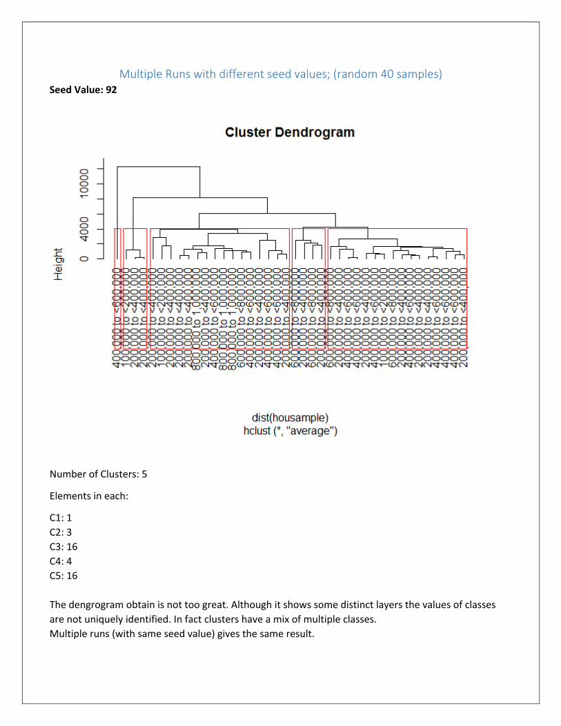
Multiple Runs with different seed values; (random 40 samples) Seed Value: 92
Number of Clusters: 5
Elements in each:
C1: 1
C2: 3
C3: 16
C4: 4
C5: 16
The dengrogram obtain is not too great. Although it shows some distinct layers the values of classes
are not uniquely identified. In fact clusters have a mix of multiple classes.
Multiple runs (with same seed value) gives the same result.

Set Value 120:
Number of Clusters: 5
Elements in each:
C1: 1
C2: 2
C3: 2
C4: 5
C5: 30
The dengrogram obtain is not too great.
Multiple runs (with same seed value) gives the same result.
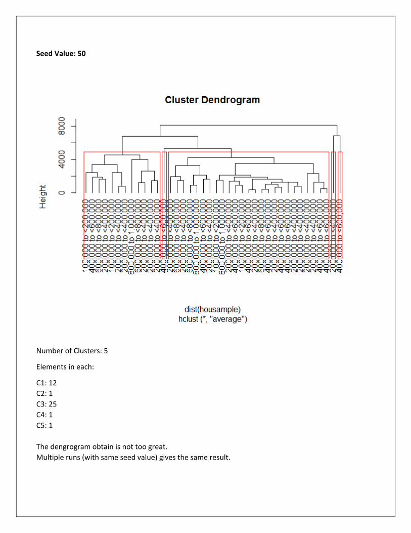
Seed Value: 50
Number of Clusters: 5
Elements in each:
C1: 12
C2: 1
C3: 25
C4: 1
C5: 1
The dengrogram obtain is not too great.
Multiple runs (with same seed value) gives the same result.

Seed Value=75
Number of Clusters: 5
Elements in each:
C1: 1
C2: 2
C3: 1
C4: 2
C5: 35
The dengrogram obtain is not too great.
Multiple runs (with same seed value) gives the same result.

We tried with three clusters as well, results didn’t improve. Below is one example.
Cut tree into 3 clusters:
Cut tree into 7 clusters:

We even tried three and seven clusters with multiple seeds. However, considering clusters of size 3,5
and 7, none of them work well for our model.
Considering all data points:
All the data points gives a practically unreadable dendogram.
Number of Clusters: 5
Density Based Clustering eps: reachability distance, which defines the size of neighborhood; (=0.42)
MinPts: minimum number of points. (=10)
We varied the values of eps and MinPts till we got appropriate clusters.
Trial1: (eps=0.42, MinPts=10) Check Clustering against actual price
> table(hou$Price, ds$cluster) 0 1 2 3 100,000 to <200,000 276 36 16 0 200,000 to <400,000 1313 0 0 16 400,000 to <600,000 1009 0 0 0 600,000 to <800,000 511 0 0 0
800,000 to 1,000,000 247 0 0 0
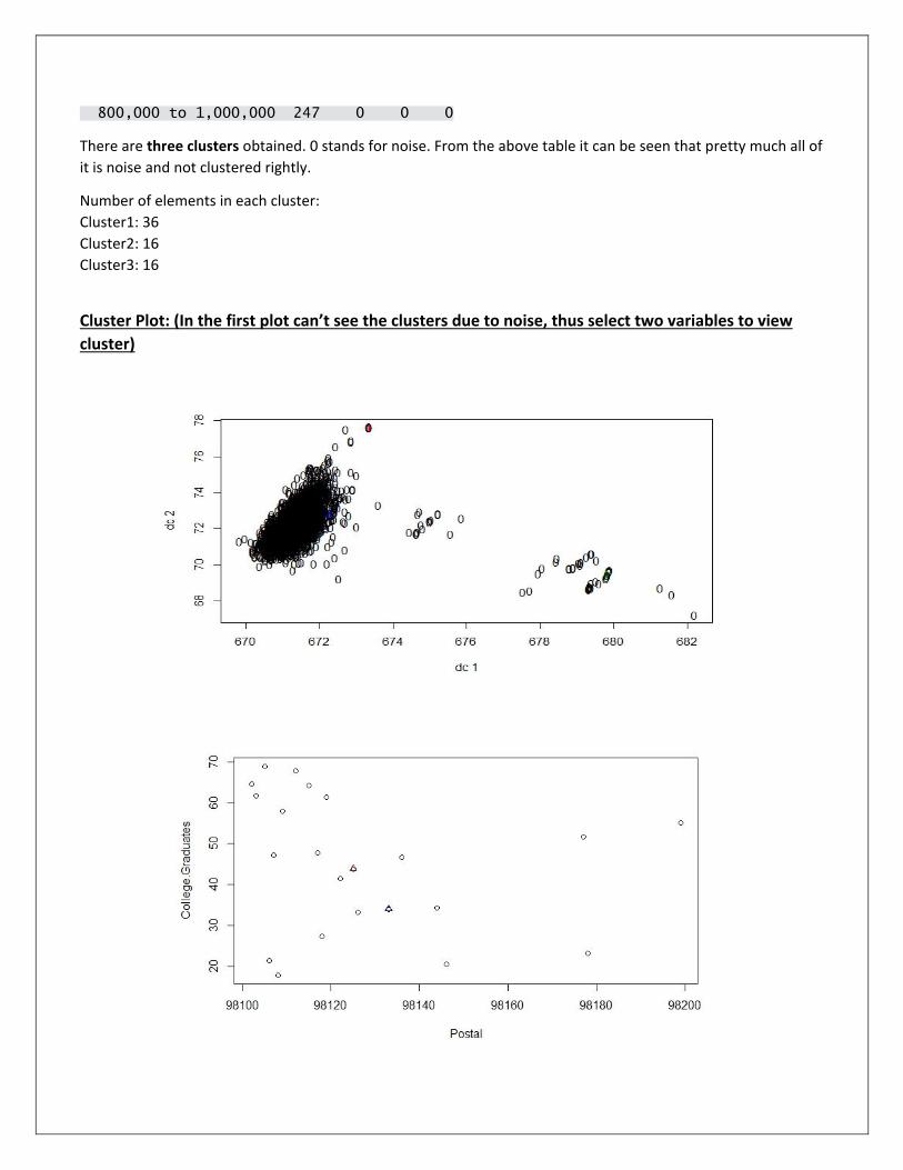
There are three clusters obtained. 0 stands for noise. From the above table it can be seen that pretty much all of
it is noise and not clustered rightly.
Number of elements in each cluster:
Cluster1: 36
Cluster2: 16
Cluster3: 16
Cluster Plot: (In the first plot can’t see the clusters due to noise, thus select two variables to view
cluster)

Cluster=3 (eps=0.2, MinPts=10)
Check Clustering against actual price
> table(hou$Price, ds$cluster) 0 1 2 3 >600,000 758 0 0 0 100,000 to <300,000 851 36 16 16 300,000 to <600,000 1747 0 0 0
There are three clusters obtained. 0 stands for noise. From the above table it can be seen that there are many
point classified as noise. However, it can be seen that the three clusters identify the class ‘100,000 to <300,000’.
Further looking into the data one reason this happens is that there are majority variables in that range.
Number of elements in each cluster:
Cluster1: 36
Cluster2: 16
Cluster3: 16
Values doesn’t change with multiple runs. Also the above identified values of eps and MinPts best identifies the
cluster size 3.
Cluster Plot: (In the first plot can’t see the clusters due to noise, thus select two variables to view
cluster)
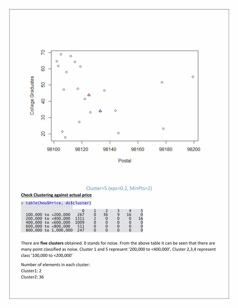
Cluster=5 (eps=0.2, MinPts=2) Check Clustering against actual price
> table(hou$Price, ds$cluster) 0 1 2 3 4 5 100,000 to <200,000 267 0 36 9 16 0 200,000 to <400,000 1311 2 0 0 0 16 400,000 to <600,000 1009 0 0 0 0 0 600,000 to <800,000 511 0 0 0 0 0 800,000 to 1,000,000 247 0 0 0 0 0
There are five clusters obtained. 0 stands for noise. From the above table it can be seen that there are
many point classified as noise. Cluster 1 and 5 represent ‘200,000 to <400,000’, Cluster 2,3,4 represent
class ‘100,000 to <200,000’
Number of elements in each cluster:
Cluster1: 2
Cluster2: 36

Cluster3: 9
Cluster4: 16
Cluster5: 16
Values don’t change with multiple runs. Also the above identified values of eps and MinPts best
identifies the cluster size 5.
Cluster Plot: (In the first plot can’t see the clusters due to noise, thus select two variables to view
cluster)

We tried varying eps and MinPts to get 7 clusters, however, in spite of trying different ways 7
clusters could not be obtained.
Mixture Model Clustering
# By default, the models considered are:
# "EII": spherical, equal volume
# "VII": spherical, unequal volume
# "EEI": diagonal, equal volume and shape
# "VEI": diagonal, varying volume, equal shape
# "EVI": diagonal, equal volume, varying shape
# "VVI": diagonal, varying volume and shape
# "EEE": ellipsoidal, equal volume, shape, and orientation
# "EEV": ellipsoidal, equal volume and equal shape
# "VEV": ellipsoidal, equal shape
# "VVV": ellipsoidal, varying volume, shape, and orientation
When we print the clusters in Mclust, we get 5 clusters with 72, 58, 603, 346, and 632 respectively.
(Also by now, we were aware that 5 clusters gives better results.)


The results obtained through various methods of clustering shows that this method does not suit our
model.
Question 4: Comparison of All classification Models Naïve Bayes
> modelNB<-train(Var,Price,method="nb",trControl=ctrl2) > modelNB Naive Bayes 5641 samples 15 predictor 5 classes: '1', '2', '3', '4', '5' No pre-processing Resampling: Cross-Validated (5 fold, repeated 3 times) Summary of sample sizes: 4512, 4513, 4513, 4513, 4513, 4513, ... Resampling results across tuning parameters: usekernel Accuracy Kappa Accuracy SD Kappa SD FALSE 0.4615024 0.3266840 0.01298926 0.01570184 TRUE 0.4976675 0.3520163 0.01114322 0.01458519 Tuning parameter 'fL' was held constant at a value of 0 Accuracy was used to select the optimal model using the largest value. The final values used for the model were fL = 0 and usekernel = TRUE. > varImp(modelNB) ROC curve variable importance variables are sorted by maximum importance across the classes X1 X2 X3 X4 X5 Sqft_Area 100.000 78.471 69.499 81.326 100.000 College.Graduates 99.299 73.865 68.284 85.861 99.299 Bath 76.251 55.191 47.273 50.985 76.251 Envi 63.406 52.552 31.531 45.462 63.406 Bed 61.850 32.924 31.324 49.915 61.850 Crime 53.431 27.903 42.319 53.431 49.409 MedIncome 50.713 31.872 31.974 46.674 50.713 Lot_Area 39.688 17.894 26.447 39.688 32.859 Age 21.714 17.406 16.976 18.250 21.714 SchoolType 20.085 6.556 1.425 20.085 5.782 SchoolTSRatio 9.356 12.711 3.998 9.956 12.711 MedAge 8.136 12.278 7.579 7.695 12.278 School 10.053 6.925 10.053 8.734 6.479 SchoolDist 8.046 4.993 8.046 2.487 1.172 Population 6.369 0.000 3.926 4.288 6.369
Bagged CART
> modeltreebag Bagged CART 5641 samples 15 predictor 5 classes: '1', '2', '3', '4', '5' No pre-processing

Resampling: Cross-Validated (5 fold, repeated 3 times) Summary of sample sizes: 4513, 4513, 4512, 4513, 4513, 4512, ... Resampling results Accuracy Kappa Accuracy SD Kappa SD 0.5624875 0.4442495 0.01139347 0.0141253
> varImp(modeltreebag) Loading required package: rpart treebag variable importance Overall Sqft_Area 100.000 Crime 81.718 Lot_Area 56.257 SchoolDist 46.850 Age 44.139 Bath 40.686 Envi 30.678 MedIncome 27.809 College.Graduates 26.228 Bed 26.220 School 20.935 SchoolTSRatio 16.639 MedAge 10.531 SchoolType 2.515 Population 0.000
Boosted tree
> modelboost Boosted Tree 5641 samples 15 predictor 5 classes: '1', '2', '3', '4', '5' No pre-processing Resampling: Cross-Validated (5 fold, repeated 3 times) Summary of sample sizes: 4512, 4513, 4512, 4514, 4513, 4512, ... Resampling results across tuning parameters: maxdepth mstop Accuracy Kappa Accuracy SD Kappa SD 1 50 0.2291585 0.02077718 0.031432165 0.035695731 1 100 0.2291585 0.02077718 0.031432165 0.035695731 1 150 0.2291585 0.02077718 0.031432165 0.035695731 2 50 0.3013064 0.10810104 0.005847599 0.007284788 2 100 0.3047924 0.11241402 0.005246116 0.006547050 2 150 0.3053834 0.11318029 0.005390346 0.006667195 3 50 0.3159016 0.12674376 0.009504368 0.011578665 3 100 0.3161971 0.12709896 0.009155411 0.011149314 3 150 0.3176151 0.12883710 0.008830094 0.010767948 Tuning parameter 'nu' was held constant at a value of 0.1 Accuracy was used to select the optimal model using the largest value. The final values used for the model were mstop = 150, maxdepth = 3 and nu = 0.1.

ROC curve variable importance variables are sorted by maximum importance across the classes X1 X2 X3 X4 X5 Sqft_Area 100.000 78.471 69.499 81.326 100.000 College.Graduates 99.299 73.865 68.284 85.861 99.299 Bath 76.251 55.191 47.273 50.985 76.251 Envi 63.406 52.552 31.531 45.462 63.406 Bed 61.850 32.924 31.324 49.915 61.850 Crime 53.431 27.903 42.319 53.431 49.409 MedIncome 50.713 31.872 31.974 46.674 50.713 Lot_Area 39.688 17.894 26.447 39.688 32.859 Age 21.714 17.406 16.976 18.250 21.714 SchoolType 20.085 6.556 1.425 20.085 5.782 SchoolTSRatio 9.356 12.711 3.998 9.956 12.711 MedAge 8.136 12.278 7.579 7.695 12.278 School 10.053 6.925 10.053 8.734 6.479 SchoolDist 8.046 4.993 8.046 2.487 1.172 Population 6.369 0.000 3.926 4.288 6.369
Random Forest
> modelRF<-train(Var,Price,method="cforest",trControl=ctrl2) > modelRF Conditional Inference Random Forest 5641 samples 15 predictor 5 classes: '1', '2', '3', '4', '5' No pre-processing Resampling: Cross-Validated (5 fold, repeated 3 times) Summary of sample sizes: 4513, 4514, 4512, 4512, 4513, 4513, ... Resampling results across tuning parameters: mtry Accuracy Kappa Accuracy SD Kappa SD 2 0.5591785 0.4307417 0.007903753 0.01031323 4 0.5725324 0.4516815 0.011046077 0.01380493 6 0.5750742 0.4560327 0.009765662 0.01223340 Accuracy was used to select the optimal model using the largest value. The final value used for the model was mtry = 6. > varImp(modelRF) cforest variable importance Overall College.Graduates 100.000 Sqft_Area 96.352 MedIncome 24.614 Envi 22.670 Bath 16.400 Crime 16.088 MedAge 14.864 Bed 12.910 Age 8.003 Lot_Area 6.279 Population 4.594 School 2.099 SchoolType 1.914 SchoolTSRatio 1.794 SchoolDist 0.000

C5.0
> modelC5T<-train(Var,Price,method="C5.0",trControl=ctrl2) > modelC5T C5.0 5641 samples 15 predictor 5 classes: '1', '2', '3', '4', '5' No pre-processing Resampling: Cross-Validated (5 fold, repeated 3 times) Summary of sample sizes: 4513, 4512, 4513, 4513, 4513, 4512, ... Resampling results across tuning parameters: model winnow trials Accuracy Kappa Accuracy SD Kappa SD rules FALSE 1 0.5470678 0.4242252 0.018888775 0.023333316 rules FALSE 10 0.5573456 0.4353997 0.011183682 0.014116430 rules FALSE 20 0.5611285 0.4397540 0.007823437 0.009873341 rules TRUE 1 0.5468882 0.4241672 0.013072039 0.016425107 rules TRUE 10 0.5549248 0.4322402 0.009516249 0.011607689 rules TRUE 20 0.5585877 0.4364002 0.008661465 0.011349713 tree FALSE 1 0.5370804 0.4117066 0.013402980 0.016913577 tree FALSE 10 0.5575249 0.4376829 0.006943332 0.008495978 tree FALSE 20 0.5611295 0.4420514 0.005715766 0.007483465 tree TRUE 1 0.5337117 0.4076954 0.012185291 0.015243445 tree TRUE 10 0.5548658 0.4342197 0.010639957 0.013594288 tree TRUE 20 0.5593583 0.4397243 0.011664038 0.014656314 Accuracy was used to select the optimal model using the largest value. The final values used for the model were trials = 20, model = tree and winnow = FALSE. > varImp(modelC5T) C5.0 variable importance Overall College.Graduates 100.00 Sqft_Area 100.00 Lot_Area 99.91 Envi 99.37 Age 99.19 Bed 98.79 Crime 96.82 MedAge 96.59 SchoolDist 94.57 School 81.70 MedIncome 80.76 SchoolType 78.52 Bath 62.87 SchoolTSRatio 60.72 Population 0.00
Glmnet
> modelglm glmnet 5641 samples

15 predictor 5 classes: '1', '2', '3', '4', '5' No pre-processing Resampling: Cross-Validated (5 fold, repeated 3 times) Summary of sample sizes: 4513, 4513, 4513, 4513, 4512, 4513, ... Resampling results across tuning parameters: alpha lambda Accuracy Kappa Accuracy SD Kappa SD 0.10 0.1000 0.5020370 0.350606687 0.0082568582 0.010898267 0.10 0.4625 0.4517518 0.277630180 0.0050883911 0.006743518 0.10 0.8250 0.4480294 0.272412267 0.0049204788 0.006504609 0.10 1.1875 0.4434196 0.266154401 0.0042467563 0.005655392 0.10 1.5500 0.4174189 0.231280063 0.0057603367 0.007672791 0.10 1.9125 0.2449328 0.001581399 0.0019491478 0.002629668 0.10 2.2750 0.2437512 0.000000000 0.0001460981 0.000000000 0.10 2.6375 0.2437512 0.000000000 0.0001460981 0.000000000 0.10 3.0000 0.2437512 0.000000000 0.0001460981 0.000000000 0.55 0.1000 0.4687700 0.303084057 0.0047406299 0.006165991 0.55 0.4625 0.2437512 0.000000000 0.0001460981 0.000000000 0.55 0.8250 0.2437512 0.000000000 0.0001460981 0.000000000 0.55 1.1875 0.2437512 0.000000000 0.0001460981 0.000000000 0.55 1.5500 0.2437512 0.000000000 0.0001460981 0.000000000 0.55 1.9125 0.2437512 0.000000000 0.0001460981 0.000000000 0.55 2.2750 0.2437512 0.000000000 0.0001460981 0.000000000 0.55 2.6375 0.2437512 0.000000000 0.0001460981 0.000000000 0.55 3.0000 0.2437512 0.000000000 0.0001460981 0.000000000 1.00 0.1000 0.4566554 0.285460500 0.0039473410 0.005316656 1.00 0.4625 0.2437512 0.000000000 0.0001460981 0.000000000 1.00 0.8250 0.2437512 0.000000000 0.0001460981 0.000000000 1.00 1.1875 0.2437512 0.000000000 0.0001460981 0.000000000 1.00 1.5500 0.2437512 0.000000000 0.0001460981 0.000000000 1.00 1.9125 0.2437512 0.000000000 0.0001460981 0.000000000 1.00 2.2750 0.2437512 0.000000000 0.0001460981 0.000000000 1.00 2.6375 0.2437512 0.000000000 0.0001460981 0.000000000 1.00 3.0000 0.2437512 0.000000000 0.0001460981 0.000000000 Accuracy was used to select the optimal model using the largest value. The final values used for the model were alpha = 0.1 and lambda = 0.1. > varImp(modelglm) glmnet variable importance variables are sorted by maximum importance across the classes 1 2 3 4 5 Bath 0.000 25.04 39.82 50.87 100.00 Envi 33.631 33.48 39.82 41.98 51.08 Bed 5.396 39.82 39.82 49.95 43.73 SchoolDist 46.210 21.52 19.62 39.82 39.82 SchoolType 45.619 39.82 37.75 37.39 39.82 College.Graduates 33.065 36.99 40.35 41.96 45.21 MedAge 39.818 43.69 39.82 39.73 34.03 SchoolTSRatio 38.437 38.52 39.82 40.09 41.86 School 39.818 40.11 39.82 39.82 39.82 Age 39.326 39.60 39.82 39.82 40.04 Sqft_Area 39.700 39.78 39.82 39.85 39.96 Crime 39.781 39.82 39.82 39.83 39.83 MedIncome 39.815 39.82 39.82 39.82 39.82 Lot_Area 39.820 39.82 39.82 39.82 39.82 Population 39.819 39.82 39.82 39.82 39.82

SVM
> modelSVM Support Vector Machines with Radial Basis Function Kernel 5641 samples 15 predictor 5 classes: '1', '2', '3', '4', '5' No pre-processing Resampling: Cross-Validated (5 fold, repeated 3 times) Summary of sample sizes: 4514, 4512, 4513, 4513, 4512, 4513, ... Resampling results across tuning parameters: C Accuracy Kappa Accuracy SD Kappa SD 0.25 0.5500195 0.4214639 0.01214735 0.01527634 0.50 0.5562233 0.4307591 0.01047647 0.01314805 1.00 0.5613642 0.4388601 0.01061579 0.01335557 Tuning parameter 'sigma' was held constant at a value of 0.05125158 Accuracy was used to select the optimal model using the largest value. The final values used for the model were sigma = 0.05125158 and C = 1. > varImp(modelSVM) ROC curve variable importance variables are sorted by maximum importance across the classes X1 X2 X3 X4 X5 Sqft_Area 100.000 78.471 69.499 81.326 100.000 College.Graduates 99.299 73.865 68.284 85.861 99.299 Bath 76.251 55.191 47.273 50.985 76.251 Envi 63.406 52.552 31.531 45.462 63.406 Bed 61.850 32.924 31.324 49.915 61.850 Crime 53.431 27.903 42.319 53.431 49.409 MedIncome 50.713 31.872 31.974 46.674 50.713 Lot_Area 39.688 17.894 26.447 39.688 32.859 Age 21.714 17.406 16.976 18.250 21.714 SchoolType 20.085 6.556 1.425 20.085 5.782 SchoolTSRatio 9.356 12.711 3.998 9.956 12.711 MedAge 8.136 12.278 7.579 7.695 12.278 School 10.053 6.925 10.053 8.734 6.479 SchoolDist 8.046 4.993 8.046 2.487 1.172 Population 6.369 0.000 3.926 4.288 6.369
Neural networks
> modelNN Neural Network 5641 samples 15 predictor 5 classes: '1', '2', '3', '4', '5' No pre-processing Resampling: Cross-Validated (5 fold, repeated 3 times) Summary of sample sizes: 4513, 4513, 4513, 4512, 4513, 4513, ... Resampling results across tuning parameters: size decay Accuracy Kappa Accuracy SD Kappa SD

1 0e+00 0.2630170 0.028241956 0.039462924 0.053039144 1 1e-04 0.2449328 0.002466057 0.003174852 0.006566703 1 1e-01 0.2641392 0.029882336 0.050174063 0.067296455 3 0e+00 0.2560977 0.020937996 0.020353386 0.027211100 3 1e-04 0.2710456 0.040569768 0.039030407 0.051771038 3 1e-01 0.3058417 0.087152176 0.058017594 0.076520735 5 0e+00 0.2626024 0.030591797 0.025633319 0.032564723 5 1e-04 0.2588796 0.024884554 0.027948045 0.037201053 5 1e-01 0.3277364 0.117896048 0.079093067 0.104216261 Accuracy was used to select the optimal model using the largest value. The final values used for the model were size = 5 and decay = 0.1.
Compare NB, Random Forest and SVM > results<-resamples(list(NB=modelNB,RF=modelRF,SVM=modelSVM)) > summary(results) Call: summary.resamples(object = results) Models: NB, RF, SVM Number of resamples: 15 Accuracy Min. 1st Qu. Median Mean 3rd Qu. Max. NA's NB 0.4805 0.4889 0.4991 0.4977 0.5055 0.5177 0 RF 0.5559 0.5696 0.5793 0.5751 0.5831 0.5847 0 SVM 0.5430 0.5534 0.5612 0.5614 0.5698 0.5798 0 Kappa Min. 1st Qu. Median Mean 3rd Qu. Max. NA's NB 0.3283 0.3404 0.3549 0.3520 0.3621 0.3782 0 RF 0.4312 0.4491 0.4624 0.4560 0.4653 0.4683 0 SVM 0.4158 0.4286 0.4377 0.4389 0.4495 0.4617 0
Compare boosted trees, random forest model and C5.0
> results1<-resamples(list(NB=modelNB,RF=modelRF,SVM=modelSVM)) > summary(results1) Call: summary.resamples(object = results1) Models: NB, RF, SVM Number of resamples: 15 Accuracy Min. 1st Qu. Median Mean 3rd Qu. Max. NA's NB 0.4805 0.4889 0.4991 0.4977 0.5055 0.5177 0 RF 0.5559 0.5696 0.5793 0.5751 0.5831 0.5847 0 SVM 0.5430 0.5534 0.5612 0.5614 0.5698 0.5798 0 Kappa Min. 1st Qu. Median Mean 3rd Qu. Max. NA's NB 0.3283 0.3404 0.3549 0.3520 0.3621 0.3782 0 RF 0.4312 0.4491 0.4624 0.4560 0.4653 0.4683 0 SVM 0.4158 0.4286 0.4377 0.4389 0.4495 0.4617 0


Compare between treebag, boost, C5.0 and Randomforest
> results<-resamples(list(Bag=modeltreebag,Boost=modelboost,RF=modelRF,C5=modelC5T)) > summary(results) Call: summary.resamples(object = results) Models: Bag, Boost, RF, C5 Number of resamples: 15 Accuracy Min. 1st Qu. Median Mean 3rd Qu. Max. NA's Bag 0.5417 0.5529 0.5660 0.5625 0.5702 0.5828 0 Boost 0.3047 0.3119 0.3156 0.3168 0.3196 0.3336 0 RF 0.5559 0.5696 0.5793 0.5751 0.5831 0.5847 0 C5 0.5537 0.5578 0.5598 0.5611 0.5638 0.5745 0 Kappa Min. 1st Qu. Median Mean 3rd Qu. Max. NA's Bag 0.4190 0.4327 0.4486 0.4442 0.4541 0.4703 0 Boost 0.1116 0.1213 0.1262 0.1277 0.1317 0.1481 0 RF 0.4312 0.4491 0.4624 0.4560 0.4653 0.4683 0 C5 0.4320 0.4371 0.4410 0.4421 0.4453 0.4593 0

Comparison between random forest, glmnet, SVM and Neural network
> results<-resamples(list(RF=modelRF,glm=modelglm,SVM=modelSVM,NN=modelNN)) > summary(results) Call: summary.resamples(object = results) Models: RF, glm, SVM, NN Number of resamples: 15 Accuracy Min. 1st Qu. Median Mean 3rd Qu. Max. NA's RF 0.5559 0.5696 0.5793 0.5751 0.5831 0.5847 0 glm 0.4885 0.4982 0.4991 0.5020 0.5078 0.5155 0 SVM 0.5430 0.5534 0.5612 0.5614 0.5698 0.5798 0 NN 0.2453 0.2614 0.2958 0.3277 0.3765 0.4672 0 Kappa Min. 1st Qu. Median Mean 3rd Qu. Max. NA's

RF 0.43120 0.44910 0.46240 0.4560 0.4653 0.4683 0 glm 0.33250 0.34510 0.34700 0.3506 0.3584 0.3682 0 SVM 0.41580 0.42860 0.43770 0.4389 0.4495 0.4617 0 NN 0.01008 0.03009 0.08621 0.1179 0.1796 0.3022 0

Regression Models
SVM
Model 1: PCA & SVM Linear kernel
> cor(pred,testPrice) [1] 0.74485 > rmse(pred, testPrice) [1] 285026.8
Model2: SVM linear kernel without PCA
> cor(hou_pred,test$Price) [,1] [1,] 0.760138 > rmse(hou_pred[,1],test$Price) [1] 241068

Model3: PCA & SVM polynomial kernel > cor(pred,testPrice) [1] 0.7961072 > rmse(pred, testPrice) [1] 250009.5
Model4: PCA & SVM radial kernel
> cor(pred2,testPrice) [1] 0.7916535 > rmse(pred2, testPrice) [1] 254747.9
Model5: SVM radial kernel without PCA
> cor(hou_pred,test$Price) [,1] [1,] 0.8395208 > rmse(hou_pred[,1],test$Price) [1] 200664.7
Model6: SVM anova kernel without PCA > cor(hou_pred,test$Price) [,1] [1,] -0.4300198 > rmse(hou_pred[,1],test$Price) [1] 386103786
Model7: Splitting with outcome SVM Linear kernel without PCA > cor(hou_pred,test$Price) [,1] [1,] 0.7776012 > rmse(hou_pred[,1],test$Price) [1] 257930.9
Model8: Splitting with predictors SVM Linear kernel without PCA
> cor(hou_pred,test$Price) [,1] [1,] 0.760138 > rmse(hou_pred[,1],test$Price) [1] 241068
Model9: Splitting with outcome SVM Radial kernel without PCA > cor(hou_pred,test$Price) [,1] [1,] 0.8389752 > rmse(hou_pred[,1],test$Price) [1] 201006.5

Model10: Splitting with predictors SVM Radial kernel without PCA
> cor(hou_pred,test$Price) [,1] [1,] 0.8761623 > rmse(hou_pred[,1],test$Price) [1] 198513.1
Neural Network Normalized so we don’t use rmse to evaluate the result
Model 1: neuralnet, One layer one node, Activation function: Logistic function ∅(ε) =1
1+exp(−𝜀)
> cor(test$Price,pred_price) [,1] [1,] 0.8339124945
Model 2: neuralnet, One layer three node, Activation function: Logistic function ∅(ε) =1
1+exp(−𝜀)
> cor(test$Price,pred_price) [,1] [1,] 0.8059231932
Model 3: neuralnet, two layers c=(3,2), Activation function: Logistic function ∅(ε) =1
1+exp(−𝜀)
> cor(test$Price,pred_price) [,1] [1,] 0.7838898422
Model 4: neuralnet, two layers c=(5,3,3), Activation function: Logistic function ∅(ε) =1
1+exp(−𝜀)
> cor(test$Price,pred_price) [,1] [1,] 0.745629228
Model 5: neuralnet, one layer with two nodes, Activation function: Tanh function f(z) = tanh(z) =𝑒𝑧−𝑒𝑧
𝑒𝑧+𝑒𝑧
> cor(test$Price,pred_price) [,1] [1,] 0.8074823746
Model 6: neuralnet, two layers c=(3,1), Activation function: Tanh function f(z) = tanh(z) =𝑒𝑧−𝑒𝑧
𝑒𝑧+𝑒𝑧
> cor(test$Price,pred_price) [,1]
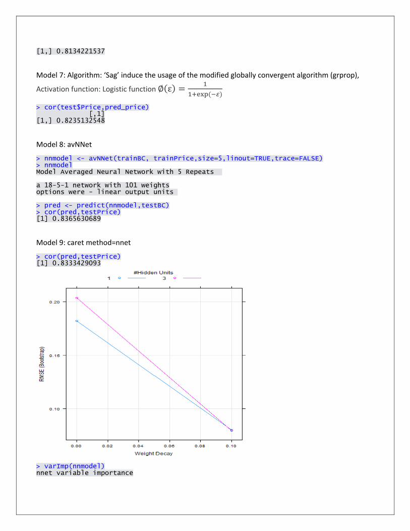
[1,] 0.8134221537
Model 7: Algorithm: ‘Sag’ induce the usage of the modified globally convergent algorithm (grprop),
Activation function: Logistic function ∅(ε) =1
1+exp(−𝜀)
> cor(test$Price,pred_price) [,1] [1,] 0.8235132548
Model 8: avNNet
> nnmodel <- avNNet(trainBC, trainPrice,size=5,linout=TRUE,trace=FALSE) > nnmodel Model Averaged Neural Network with 5 Repeats a 18-5-1 network with 101 weights options were - linear output units > pred <- predict(nnmodel,testBC) > cor(pred,testPrice) [1] 0.8365630689
Model 9: caret method=nnet
> cor(pred,testPrice) [1] 0.8333429093
> varImp(nnmodel) nnet variable importance

Overall Sqft_Area 100.000000 Bath 43.086821 MedAge 30.728180 Envi 26.503750 Lot_Area 24.902230 College.Graduates 22.397486 MedIncome 17.995196 SchoolDist 15.631032 SchoolRating 13.549307 Crime 11.729848 Postal 10.563251 School 9.374383 SchoolTSRatio 8.043920 Population 7.638119 Rank 6.985514 SchoolType 6.696112 Age 4.333750 Bed 0.000000
Regression Comparison > modelSVMLinear Support Vector Machines with Linear Kernel 5641 samples 15 predictor No pre-processing Resampling: Cross-Validated (5 fold, repeated 3 times) Summary of sample sizes: 4512, 4513, 4513, 4513, 4513, 4513, ... Resampling results RMSE Rsquared RMSE SD Rsquared SD 0.1471002022 0.5999477232 0.005009685209 0.02718982684 Tuning parameter 'C' was held constant at a value of 1
> varImp(modelSVMLinear) loess r-squared variable importance Overall Sqft_Area 100.0000000 College.Graduates 82.7538147 Bath 51.1962278 Envi 35.6840267 Crime 33.4441930 Bed 32.9283352 MedIncome 31.4933671 Lot_Area 14.0719613 MedAge 4.8664026 Age 3.1121048 SchoolType 1.7820851 Population 0.5485360 SchoolDist 0.3925719 SchoolTSRatio 0.2971874 School 0.0000000

> modelSVMPoly<- train(Var,Price,method = "svmPoly",trControl = ctrl2) > modelSVMPoly Support Vector Machines with Polynomial Kernel 5641 samples 15 predictor No pre-processing Resampling: Cross-Validated (5 fold, repeated 3 times) Summary of sample sizes: 4513, 4512, 4513, 4513, 4513, 4512, ... Resampling results across tuning parameters: degree scale C RMSE Rsquared RMSE SD Rsquared SD 1 0.001 0.25 0.1566427647 0.5820621175 0.004429881254 0.02403241936 1 0.001 0.50 0.1510080174 0.5898070310 0.004393366226 0.02376442121 1 0.001 1.00 0.1485760038 0.5949888565 0.004543168950 0.02378689302 1 0.010 0.25 0.1474256134 0.5984569453 0.004567268014 0.02361883112 1 0.010 0.50 0.1472122712 0.5991412412 0.004622792592 0.02373725587 1 0.010 1.00 0.1471916610 0.5992957230 0.004642187974 0.02379333257 1 0.100 0.25 0.1471662112 0.5994696539 0.004645148137 0.02373262562 1 0.100 0.50 0.1471605503 0.5995593481 0.004639455565 0.02367802163 1 0.100 1.00 0.1471605854 0.5995757353 0.004639757847 0.02368661903 2 0.001 0.25 0.1509352814 0.5902515619 0.004385477684 0.02372284041 2 0.001 0.50 0.1484338295 0.5958382717 0.004546753166 0.02378108675 2 0.001 1.00 0.1472955742 0.5994879136 0.004603988831 0.02372847918 2 0.010 0.25 0.1439351331 0.6173543292 0.005063695188 0.02447585706 2 0.010 0.50 0.1429713471 0.6221105988 0.005189393001 0.02461145186 2 0.010 1.00 0.1423579146 0.6253238558 0.005359853853 0.02513552723 2 0.100 0.25 0.1404799973 0.6357725448 0.005697832114 0.02766512014 2 0.100 0.50 0.1403523157 0.6366087170 0.005798508204 0.02807992182 2 0.100 1.00 0.1403800724 0.6366184355 0.005875507693 0.02830768463 3 0.001 0.25 0.1490936346 0.5945088207 0.004525263117 0.02388895252 3 0.001 0.50 0.1474606056 0.5992971481 0.004604203123 0.02386723715 3 0.001 1.00 0.1465328801 0.6031955086 0.004681296793 0.02383823631 3 0.010 0.25 0.1412998751 0.6306364078 0.004839212810 0.02343047579 3 0.010 0.50 0.1399899821 0.6373135744 0.004582224588 0.02285212820 3 0.010 1.00 0.1386186065 0.6443611055 0.004334712951 0.02233070740 3 0.100 0.25 0.1491537921 0.6128232823 0.025149660514 0.09189555329 3 0.100 0.50 0.1599580374 0.5765878941 0.031438008134 0.10782684085 3 0.100 1.00 0.1703413719 0.5466125939 0.037137191397 0.11894819055 RMSE was used to select the optimal model using the smallest value. The final values used for the model were degree = 3, scale = 0.01 and C = 1. > varImp(modelSVMPoly) loess r-squared variable importance Overall Sqft_Area 100.0000000 College.Graduates 82.7538147 Bath 51.1962278 Envi 35.6840267 Crime 33.4441930 Bed 32.9283352 MedIncome 31.4933671 Lot_Area 14.0719613 MedAge 4.8664026 Age 3.1121048 SchoolType 1.7820851 Population 0.5485360 SchoolDist 0.3925719
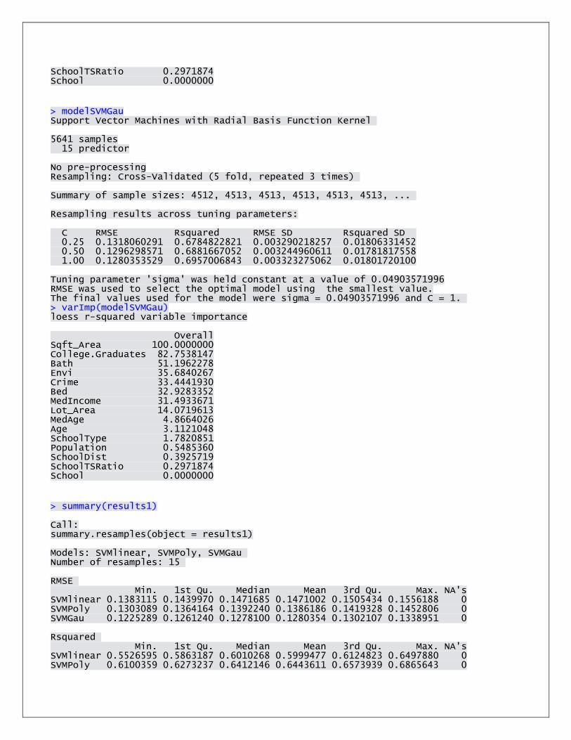
SchoolTSRatio 0.2971874 School 0.0000000
> modelSVMGau Support Vector Machines with Radial Basis Function Kernel 5641 samples 15 predictor No pre-processing Resampling: Cross-Validated (5 fold, repeated 3 times) Summary of sample sizes: 4512, 4513, 4513, 4513, 4513, 4513, ... Resampling results across tuning parameters: C RMSE Rsquared RMSE SD Rsquared SD 0.25 0.1318060291 0.6784822821 0.003290218257 0.01806331452 0.50 0.1296298571 0.6881667052 0.003244960611 0.01781817558 1.00 0.1280353529 0.6957006843 0.003323275062 0.01801720100 Tuning parameter 'sigma' was held constant at a value of 0.04903571996 RMSE was used to select the optimal model using the smallest value. The final values used for the model were sigma = 0.04903571996 and C = 1. > varImp(modelSVMGau) loess r-squared variable importance Overall Sqft_Area 100.0000000 College.Graduates 82.7538147 Bath 51.1962278 Envi 35.6840267 Crime 33.4441930 Bed 32.9283352 MedIncome 31.4933671 Lot_Area 14.0719613 MedAge 4.8664026 Age 3.1121048 SchoolType 1.7820851 Population 0.5485360 SchoolDist 0.3925719 SchoolTSRatio 0.2971874 School 0.0000000
> summary(results1) Call: summary.resamples(object = results1) Models: SVMlinear, SVMPoly, SVMGau Number of resamples: 15 RMSE Min. 1st Qu. Median Mean 3rd Qu. Max. NA's SVMlinear 0.1383115 0.1439970 0.1471685 0.1471002 0.1505434 0.1556188 0 SVMPoly 0.1303089 0.1364164 0.1392240 0.1386186 0.1419328 0.1452806 0 SVMGau 0.1225289 0.1261240 0.1278100 0.1280354 0.1302107 0.1338951 0 Rsquared Min. 1st Qu. Median Mean 3rd Qu. Max. NA's SVMlinear 0.5526595 0.5863187 0.6010268 0.5999477 0.6124823 0.6497880 0 SVMPoly 0.6100359 0.6273237 0.6412146 0.6443611 0.6573939 0.6865643 0

SVMGau 0.6654565 0.6843478 0.6962391 0.6957007 0.7067423 0.7261745 0

> modelavNN<-train(Var,Price,method="avNNet",trace=FALSE,trControl=ctrl2) > modelavNN Model Averaged Neural Network 5641 samples 15 predictor No pre-processing Resampling: Cross-Validated (5 fold, repeated 3 times) Summary of sample sizes: 4513, 4512, 4513, 4513, 4513, 4514, ... Resampling results across tuning parameters: size decay RMSE Rsquared RMSE SD Rsquared SD 1 0.0000 0.1442407843 0.6183253633 0.004858524546 0.02557004181 1 0.0001 0.1439102750 0.6183239790 0.005429549190 0.02553624430 1 0.1000 0.1433408820 0.6178789468 0.005034255393 0.02503575869

3 0.0000 0.1363835482 0.6573437912 0.005116149222 0.02340869139 3 0.0001 0.1359264681 0.6562175619 0.005145391664 0.02422242718 3 0.1000 0.1398453236 0.6363512617 0.005074969443 0.02430218281 5 0.0000 0.1360655744 0.6759521674 0.008331072349 0.02317691325 5 0.0001 0.1324807687 0.6750067232 0.005646282898 0.02396110947 5 0.1000 0.1391465116 0.6399237796 0.005038380773 0.02399215137 Tuning parameter 'bag' was held constant at a value of FALSE RMSE was used to select the optimal model using the smallest value. The final values used for the model were size = 5, decay = 0.0001 and bag = FALSE. > varImp(modelavNN) loess r-squared variable importance Overall Sqft_Area 100.0000000 College.Graduates 82.7538147 Bath 51.1962278 Envi 35.6840267 Crime 33.4441930 Bed 32.9283352 MedIncome 31.4933671 Lot_Area 14.0719613 MedAge 4.8664026 Age 3.1121048 SchoolType 1.7820851 Population 0.5485360 SchoolDist 0.3925719 SchoolTSRatio 0.2971874 School 0.0000000
> modelNN Neural Network 5641 samples 15 predictor No pre-processing Resampling: Cross-Validated (5 fold, repeated 3 times) Summary of sample sizes: 4512, 4513, 4513, 4513, 4513, 4514, ... Resampling results across tuning parameters: size decay RMSE Rsquared RMSE SD Rsquared SD 1 0.0000 0.1430968287 0.6189702451 0.004063692748 0.01537837268 1 0.0001 0.1431089253 0.6189154851 0.004028925793 0.01525104329 1 0.1000 0.1432205464 0.6186248942 0.003992856443 0.01546359267 3 0.0000 0.1448759403 0.6418808162 0.023409157755 0.01523849922 3 0.0001 0.1394457372 0.6382139611 0.004916504231 0.01984821939 3 0.1000 0.1398189346 0.6365474556 0.004240222978 0.01657643623 5 0.0000 0.1347891667 0.6622979542 0.004684207530 0.01866600785 5 0.0001 0.1367491986 0.6521490277 0.005675859037 0.02572711316 5 0.1000 0.1390072819 0.6407683902 0.004069146715 0.01643053366 RMSE was used to select the optimal model using the smallest value. The final values used for the model were size = 5 and decay = 0. > varImp(modelNN) nnet variable importance Overall Age 100.000000 Lot_Area 99.102320 Sqft_Area 85.225457

MedAge 50.562629 Bath 50.551308 MedIncome 47.945716 College.Graduates 31.548933 Population 24.038945 SchoolType 21.028919 Envi 20.147681 Crime 17.888144 Bed 15.652234 SchoolDist 15.529903 School 6.422972 SchoolTSRatio 0.000000
> modelpcaNN<-train(Var,Price,method="pcaNNet",trace=FALSE,trControl=ctrl2) > modelpcaNN Neural Networks with Feature Extraction 5641 samples 15 predictor No pre-processing Resampling: Cross-Validated (5 fold, repeated 3 times) Summary of sample sizes: 4512, 4513, 4513, 4513, 4513, 4512, ... Resampling results across tuning parameters: size decay RMSE Rsquared RMSE SD Rsquared SD 1 0.0000 0.1437670259 0.6152324800 0.004908875706 0.02404207231 1 0.0001 0.1437674784 0.6152306269 0.004908467175 0.02404270253 1 0.1000 0.1440596400 0.6138001185 0.004739665036 0.02312499048 3 0.0000 0.1391298140 0.6396471464 0.004974695225 0.02326461766 3 0.0001 0.1400310595 0.6349572666 0.005049410350 0.02440829999 3 0.1000 0.1383566964 0.6435292252 0.004910930166 0.02363679943 5 0.0000 0.1368383556 0.6514404439 0.005405281347 0.02651476398 5 0.0001 0.1360422194 0.6554949049 0.005004692178 0.02345590259 5 0.1000 0.1355870170 0.6576442632 0.004602091927 0.02109622283 RMSE was used to select the optimal model using the smallest value. The final values used for the model were size = 5 and decay = 0.1. > varImp(modelpcaNN) loess r-squared variable importance Overall Sqft_Area 100.0000000 College.Graduates 82.7538147 Bath 51.1962278 Envi 35.6840267 Crime 33.4441930 Bed 32.9283352 MedIncome 31.4933671 Lot_Area 14.0719613 MedAge 4.8664026 Age 3.1121048 SchoolType 1.7820851 Population 0.5485360 SchoolDist 0.3925719 SchoolTSRatio 0.2971874 School 0.0000000
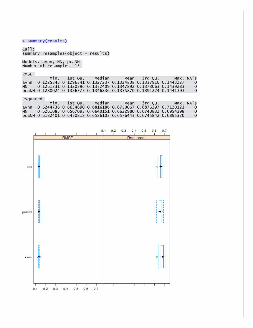
> summary(results) Call: summary.resamples(object = results) Models: avnn, NN, pcaNN Number of resamples: 15 RMSE Min. 1st Qu. Median Mean 3rd Qu. Max. NA's avnn 0.1225343 0.1296341 0.1327237 0.1324808 0.1337910 0.1443227 0 NN 0.1261231 0.1320396 0.1352409 0.1347892 0.1373063 0.1439283 0 pcaNN 0.1280024 0.1326375 0.1346836 0.1355870 0.1391224 0.1441393 0 Rsquared Min. 1st Qu. Median Mean 3rd Qu. Max. NA's avnn 0.6244736 0.6634690 0.6816186 0.6750067 0.6876297 0.7120121 0 NN 0.6261085 0.6567093 0.6640151 0.6622980 0.6740832 0.6954398 0 pcaNN 0.6182401 0.6450818 0.6586103 0.6576443 0.6745842 0.6895320 0

> modelglmboost Boosted Generalized Linear Model 5641 samples 15 predictor No pre-processing Resampling: Cross-Validated (5 fold, repeated 3 times) Summary of sample sizes: 4514, 4513, 4512, 4513, 4512, 4513, ... Resampling results across tuning parameters: mstop RMSE Rsquared RMSE SD Rsquared SD 50 0.1518451313 0.5831508787 0.003766052676 0.02818644018 100 0.1476325363 0.5974334064 0.004285973716 0.02692213146 150 0.1467641892 0.6001913276 0.004485016739 0.02638363524 Tuning parameter 'prune' was held constant at a value of no RMSE was used to select the optimal model using the smallest value.

The final values used for the model were mstop = 150 and prune = no. > varImp(modelglmboost) loess r-squared variable importance Overall Sqft_Area 100.0000000 College.Graduates 82.7538147 Bath 51.1962278 Envi 35.6840267 Crime 33.4441930 Bed 32.9283352 MedIncome 31.4933671 Lot_Area 14.0719613 MedAge 4.8664026 Age 3.1121048 SchoolType 1.7820851 Population 0.5485360 SchoolDist 0.3925719 SchoolTSRatio 0.2971874 School 0.0000000
> modellm Linear Regression 5641 samples 15 predictor No pre-processing Resampling: Cross-Validated (5 fold, repeated 3 times) Summary of sample sizes: 4512, 4513, 4513, 4513, 4513, 4514, ... Resampling results RMSE Rsquared RMSE SD Rsquared SD 0.1463922249 0.6016901809 0.00542678064 0.03245792673 > varImp(modellm) lm variable importance Overall Sqft_Area 100.000000 College.Graduates 76.459068 Population 37.887922 Envi 31.455262 Bath 26.414385 SchoolTSRatio 24.600588 Lot_Area 22.515233 Age 16.311331 MedAge 15.486737 School 12.229639 SchoolType 10.099096 Crime 8.718225 MedIncome 4.920911 SchoolDist 1.623632 Bed 0.000000
> modelglm glmnet 5641 samples

15 predictor No pre-processing Resampling: Cross-Validated (5 fold, repeated 3 times) Summary of sample sizes: 4512, 4513, 4514, 4513, 4512, 4512, ... Resampling results across tuning parameters: alpha lambda RMSE Rsquared RMSE SD Rsquared SD 0.10 0.1000 0.1556796619 0.5889892292 0.003203018760 0.01655369347 0.10 0.4625 0.1970868533 0.5595059616 0.004022137698 0.01946358987 0.10 0.8250 0.2198780123 0.5431975421 0.003957664764 0.02100859574 0.10 1.1875 0.2298261604 0.4390601748 0.003829352730 0.02509214294 0.10 1.5500 0.2317165010 NaN 0.003661417872 NA 0.10 1.9125 0.2317165010 NaN 0.003661417872 NA 0.10 2.2750 0.2317165010 NaN 0.003661417872 NA 0.10 2.6375 0.2317165010 NaN 0.003661417872 NA 0.10 3.0000 0.2317165010 NaN 0.003661417872 NA 0.55 0.1000 0.1789845586 0.5485412426 0.004096874417 0.01944059662 0.55 0.4625 0.2317165010 NaN 0.003661417872 NA 0.55 0.8250 0.2317165010 NaN 0.003661417872 NA 0.55 1.1875 0.2317165010 NaN 0.003661417872 NA 0.55 1.5500 0.2317165010 NaN 0.003661417872 NA 0.55 1.9125 0.2317165010 NaN 0.003661417872 NA 0.55 2.2750 0.2317165010 NaN 0.003661417872 NA 0.55 2.6375 0.2317165010 NaN 0.003661417872 NA 0.55 3.0000 0.2317165010 NaN 0.003661417872 NA 1.00 0.1000 0.2055380735 0.5278939900 0.004357359584 0.02408046024 1.00 0.4625 0.2317165010 NaN 0.003661417872 NA 1.00 0.8250 0.2317165010 NaN 0.003661417872 NA 1.00 1.1875 0.2317165010 NaN 0.003661417872 NA 1.00 1.5500 0.2317165010 NaN 0.003661417872 NA 1.00 1.9125 0.2317165010 NaN 0.003661417872 NA 1.00 2.2750 0.2317165010 NaN 0.003661417872 NA 1.00 2.6375 0.2317165010 NaN 0.003661417872 NA 1.00 3.0000 0.2317165010 NaN 0.003661417872 NA RMSE was used to select the optimal model using the smallest value. The final values used for the model were alpha = 0.1 and lambda = 0.1. > varImp(modelglm) glmnet variable importance Overall Sqft_Area 100.000000 Bath 51.554241 College.Graduates 32.521337 Envi 24.873893 MedIncome 21.091434 Bed 20.170027 Crime 14.834945 Age 12.199482 SchoolTSRatio 11.902154 School 9.587050 SchoolDist 9.587050 SchoolType 9.587050 Population 5.814378 MedAge 1.812784 Lot_Area 0.000000
> summary(results) Call:

summary.resamples(object = results) Models: glmboost, lm, glm Number of resamples: 15 RMSE Min. 1st Qu. Median Mean 3rd Qu. Max. NA's glmboost 0.1406669 0.1433445 0.1464334 0.1467642 0.1500557 0.1559712 0 lm 0.1338699 0.1450716 0.1459954 0.1463922 0.1495640 0.1565299 0 glm 0.1521615 0.1535458 0.1549178 0.1556797 0.1566197 0.1645875 0 Rsquared Min. 1st Qu. Median Mean 3rd Qu. Max. NA's glmboost 0.5592761 0.5851682 0.5911342 0.6001913 0.6240403 0.6423232 0 lm 0.5436076 0.5840372 0.6024809 0.6016902 0.6172231 0.6653351 0 glm 0.5654892 0.5801327 0.5877108 0.5889892 0.5948493 0.6252723 0

> modeltreebag Bagged CART 5641 samples 15 predictor No pre-processing Resampling: Cross-Validated (5 fold, repeated 3 times) Summary of sample sizes: 4513, 4513, 4512, 4514, 4512, 4513, ... Resampling results RMSE Rsquared RMSE SD Rsquared SD 0.1468711752 0.6000819707 0.003281957828 0.02083289701 > varImp(modeltreebag) Loading required package: rpart treebag variable importance
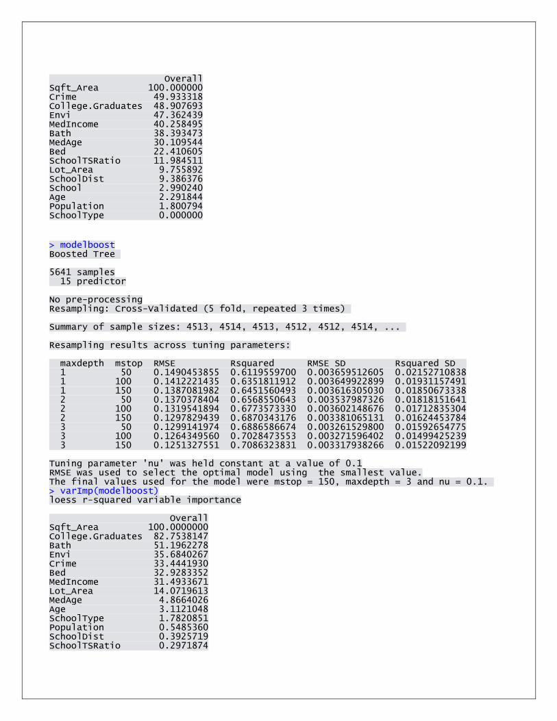
Overall Sqft_Area 100.000000 Crime 49.933318 College.Graduates 48.907693 Envi 47.362439 MedIncome 40.258495 Bath 38.393473 MedAge 30.109544 Bed 22.410605 SchoolTSRatio 11.984511 Lot_Area 9.755892 SchoolDist 9.386376 School 2.990240 Age 2.291844 Population 1.800794 SchoolType 0.000000
> modelboost Boosted Tree 5641 samples 15 predictor No pre-processing Resampling: Cross-Validated (5 fold, repeated 3 times) Summary of sample sizes: 4513, 4514, 4513, 4512, 4512, 4514, ... Resampling results across tuning parameters: maxdepth mstop RMSE Rsquared RMSE SD Rsquared SD 1 50 0.1490453855 0.6119559700 0.003659512605 0.02152710838 1 100 0.1412221435 0.6351811912 0.003649922899 0.01931157491 1 150 0.1387081982 0.6451560493 0.003616305030 0.01850673338 2 50 0.1370378404 0.6568550643 0.003537987326 0.01818151641 2 100 0.1319541894 0.6773573330 0.003602148676 0.01712835304 2 150 0.1297829439 0.6870343176 0.003381065131 0.01624453784 3 50 0.1299141974 0.6886586674 0.003261529800 0.01592654775 3 100 0.1264349560 0.7028473553 0.003271596402 0.01499425239 3 150 0.1251327551 0.7086323831 0.003317938266 0.01522092199 Tuning parameter 'nu' was held constant at a value of 0.1 RMSE was used to select the optimal model using the smallest value. The final values used for the model were mstop = 150, maxdepth = 3 and nu = 0.1. > varImp(modelboost) loess r-squared variable importance Overall Sqft_Area 100.0000000 College.Graduates 82.7538147 Bath 51.1962278 Envi 35.6840267 Crime 33.4441930 Bed 32.9283352 MedIncome 31.4933671 Lot_Area 14.0719613 MedAge 4.8664026 Age 3.1121048 SchoolType 1.7820851 Population 0.5485360 SchoolDist 0.3925719 SchoolTSRatio 0.2971874

School 0.0000000
> modelCRF Conditional Inference Random Forest 5641 samples 15 predictor No pre-processing Resampling: Cross-Validated (5 fold, repeated 3 times) Summary of sample sizes: 4513, 4513, 4513, 4513, 4512, 4513, ... Resampling results across tuning parameters: mtry RMSE Rsquared RMSE SD Rsquared SD 2 0.1584932274 0.6016451121 0.002750843150 0.01606171430 4 0.1333815548 0.6768557036 0.002953947721 0.01455815138 6 0.1284350658 0.6949495045 0.002713322586 0.01383200047 RMSE was used to select the optimal model using the smallest value. The final value used for the model was mtry = 6. > varImp(modelCRF) cforest variable importance Overall College.Graduates 100.0000000 Sqft_Area 90.3658731 Envi 19.9696139 MedIncome 19.0856859 MedAge 12.6408929 Bath 11.8764958 Crime 10.3536939 Bed 5.0099601 Age 4.0396785 Population 2.9658027 Lot_Area 2.2455409 SchoolDist 0.9589474 SchoolTSRatio 0.5632945 School 0.1160036 SchoolType 0.0000000
> modelRF Random Forest 5641 samples 15 predictor No pre-processing Resampling: Cross-Validated (5 fold, repeated 3 times) Summary of sample sizes: 4513, 4513, 4513, 4512, 4513, 4512, ... Resampling results across tuning parameters: mtry RMSE Rsquared RMSE SD Rsquared SD 2 0.1228370225 0.7237012977 0.004165306086 0.01927768143 8 0.1232090712 0.7180273534 0.004547151038 0.02034720904 15 0.1252951897 0.7082554393 0.004698949803 0.02091216882 RMSE was used to select the optimal model using the smallest value. The final value used for the model was mtry = 2.

> results<-resamples(list(treebad=modeltreebag,boost=modelboost, + CRF=modelCRF,RF=modelRF)) > summary(results) Call: summary.resamples(object = results) Models: treebad, boost, CRF, RF Number of resamples: 15 RMSE Min. 1st Qu. Median Mean 3rd Qu. Max. NA's treebad 0.1411368 0.1449034 0.1457785 0.1468712 0.1490169 0.1532344 0 boost 0.1206413 0.1231550 0.1243797 0.1251328 0.1278636 0.1309538 0 CRF 0.1242264 0.1267010 0.1284136 0.1284351 0.1304487 0.1338046 0 RF 0.1161424 0.1191386 0.1223180 0.1228370 0.1261773 0.1292430 0 Rsquared Min. 1st Qu. Median Mean 3rd Qu. Max. NA's treebad 0.5624958 0.5855010 0.6025259 0.6000820 0.6140623 0.6298769 0 boost 0.6846224 0.6992575 0.7088991 0.7086324 0.7183076 0.7363437 0 CRF 0.6699291 0.6867862 0.6963358 0.6949495 0.7049934 0.7154786 0 RF 0.6934433 0.7107682 0.7206473 0.7237013 0.7389190 0.7559046 0 > summary(results) Call: summary.resamples(object = results) Models: RF, SVM, avNNet, lm Number of resamples: 15 RMSE Min. 1st Qu. Median Mean 3rd Qu. Max. NA's RF 0.1161424 0.1191386 0.1223180 0.1228370 0.1261773 0.1292430 0 SVM 0.1225289 0.1261240 0.1278100 0.1280354 0.1302107 0.1338951 0 avNNet 0.1225343 0.1296341 0.1327237 0.1324808 0.1337910 0.1443227 0 lm 0.1338699 0.1450716 0.1459954 0.1463922 0.1495640 0.1565299 0 Rsquared Min. 1st Qu. Median Mean 3rd Qu. Max. NA's RF 0.6934433 0.7107682 0.7206473 0.7237013 0.7389190 0.7559046 0 SVM 0.6654565 0.6843478 0.6962391 0.6957007 0.7067423 0.7261745 0 avNNet 0.6244736 0.6634690 0.6816186 0.6750067 0.6876297 0.7120121 0 lm 0.5436076 0.5840372 0.6024809 0.6016902 0.6172231 0.6653351 0


Comparative analysis summary Comparison of Classification Models:
According to the comparison, SVM models with Gaussian kernel works best for our data, neural
network with preprocessing of normalization and prominent component analysis works best. In all
models, the accuracy of random forest is the best.
Comparison of Regression Models:
According to the comparison of regression models, SVM models with Gaussian kernel still works best
for our data, neural network with preprocessing of normalization and principle component analysis

works best. In comparative analysis of linear models, tree models, SVM models and neural network
models, random forest has the least RMSE (root mean square deviation) which indicate best
performance.
Others:
Meanwhile we find that when split data based on outcome or predictors, the model usually works
better than data splitting randomly.
PCA (Principle component analysis) works better for neural network however worse for SVM in our
data, which suggest more testing when using preprocessing of PCA.