Zheng Zhang, 27.05.2010 Exact Matching slide 1 Outline Graph matching – Definition – Manifold...
62
Zheng Zhang, 27.05.2010 Exact Matching slide 1 Outline • Graph matching – Definition – Manifold application areas • Exact matching – Definition – Different forms of exact matching – Necessary concepts • Algorithms for exact matching – Techniques based on tree search – Other techniques • Conclusion
-
Upload
brittany-brooke-armstrong -
Category
Documents
-
view
218 -
download
0
Transcript of Zheng Zhang, 27.05.2010 Exact Matching slide 1 Outline Graph matching – Definition – Manifold...
Zheng Zhang, 27.05.2010 Exact Matching slide 1
Outline
• Graph matching– Definition– Manifold application areas
• Exact matching– Definition– Different forms of exact matching– Necessary concepts
• Algorithms for exact matching– Techniques based on tree search– Other techniques
• Conclusion

Zheng Zhang, 27.05.2010 Exact Matching slide 2
Graph matching
• Definition:– Graph matching is the process of finding a correspondence between
the nodes and the edges of two graphs that satisfies some (more or less stringent) constraints ensuring that similar substructures in one graph are mapped to similar substructures in the other.
[D. Conte, Pasquale Foggia, Carlo Sansone, and Mario Vento. Thirty Years of Graph Matching in Pattern Recognition.]
• in comparison with matching (graph theory):– A matching or independent edge set in a graph is a set of edges without
common vertices. It may also be an entire graph consisting of edges without common vertices.
[Wikipedia]

Zheng Zhang, 27.05.2010 Exact Matching slide 3
Graph matching
• Manifold application areas– 2D and 3D image analysis– Document processing– Biometric identification– Image databases– Video analysis– Biological and biomedical applications
• Categories of matching– Exact matching– Inexact matching– Other matching problems

Zheng Zhang, 27.05.2010 Exact Matching slide 4
Exact matching
• Definition– Exact graph matching is characterized by the fact that the mapping
between the nodes of the two graphs must be edge-preserving in the sense that if two nodes in the first graph are linked by an edge, they are mapped to two nodes in the second graph that are linked by an edge as well.
• Different forms of exact matching– The most stringent form: graph isomorphism– A weaker form: subgraph isomorphism– A slightly weaker form: monomorphism– A still weaker form: homomorphism– Another interesting form: maximum common subgraph (MCS)

Zheng Zhang, 27.05.2010 Exact Matching slide 5
Necessary concepts
• Morphism– A morphism is an abstraction derived from structure-preserving
mappings between two mathematical structures. – In comparison with homomorphism: a homomorphism is a structure-
preserving map between two mathematical structures.– If a morphism f has domain X and codomain Y, we write f :X→Y. Thus
a morphism is represented by an arrow from its domain to its codomain. The collection of all morphisms from X to Y is denoted Hom(X,Y) or Mor(X,Y) .
• Isomorphism– An isomorphism is a bijective homomorphism.– An isomorphism is a morphism f :X→Y in a category for which there
exists an "inverse" f−1 :Y→X, with the property that both f−1·f = idX and f·f−1 =idY.

Zheng Zhang, 27.05.2010 Exact Matching slide 6
Necessary concepts
• Epimorphism– an surjective homomorphism
• Monomorphism– an injective homomorphism
• Endomoprphism– a homomorphism from an object
to itself
• Automoprphism– an endomorphism which is also
an isomorphisman isomorphism with itself
Homo
Mono Iso Epi
Auto
Endo

Zheng Zhang, 27.05.2010 Exact Matching slide 7
Different forms of exact matching
• Graph isomorphism – A one-to-one correspondence must be found between each node of
the first graph and each node of the second graph.– Graphs G(VG,EG) and H(VH,EH) are isomorphic if there is an invertible
F from VG to VH such that for all nodes u and v in VG, (u,v) E∈ G if and only if (F(u),F(v)) E∈ H.
4
1
23
5
4
1
23
5
C
A
B E
D

Zheng Zhang, 27.05.2010 Exact Matching slide 8
Different forms of exact matching
• Subgraph isomorphism – It requires that an isomorphism holds between one of the two
graphs and a node-induced subgraph of the other.
C
A
B E
D
3
1
2
• Monomorphism – It requires that each node of the first graph is mapped to a distinct
node of the second one, and each edge of the first graph has a corresponding edge in the second one; the second graph, however, may have both extra nodes and extra edges.

Zheng Zhang, 27.05.2010 Exact Matching slide 9
Different forms of exact matching
• Homomorphism – It drops the condition that nodes in the first graph are to be mapped
to distinct nodes of the other; hence, the correspondence can be many-to-one.
– A graph homomorphism F from Graph G(VG,EG) and H(VH,EH), is a mapping F from VG to VH such that {x,y} E∈ G implies {F(x),F(y)} E∈ H.
C
A
B E
D
3
1
2
4

Zheng Zhang, 27.05.2010 Exact Matching slide 10
Different forms of exact matching
• Maximum common subgraph (MCS) – A subgraph of the first graph is mapped to an isomorphic subgraph
of the second one.– There are two possible definitions of the problem, depending on
whether node-induced subgraphs or plain subgraphs are used.– The problem of finding the MCS of two graphs can be reduced to
the problem of finding the maximum clique (i.e. a fully connected subgraph) in a suitably defined association graph.
C
A
B E
D
3
1
2
4

Zheng Zhang, 27.05.2010 Exact Matching slide 11
Different forms of exact matching
• Properties – The matching problems are all NP-complete except for graph
isomorphism, which has not yet been demonstrated whether in NP or not.
– Exact graph matching has exponential time complexity in the worst case. However, in many PR applications the actual computation time can be still acceptable.
– Exact isomorphism is very seldom used in PR. Subgraph isomorphism and monomorphism can be effectively used in many contexts.
– The MCS problem is receiving much attention.

Zheng Zhang, 27.05.2010 Exact Matching slide 12
Algorithms for exact matching
• Techniques based on tree search – mostly based on some form of tree search with backtracking
Ullmann’s algorithmGhahraman’s algorithmVF and VF2 algorithmBron and Kerbosh’s algorithmOther algorithms for the MCS problem
• Other techniques– based on A* algorithm
Demko’s algorithm– based on group theory
Nauty algorithm


Zheng Zhang, 27.05.2010 Exact Matching slide 18
Techniques based on tree search
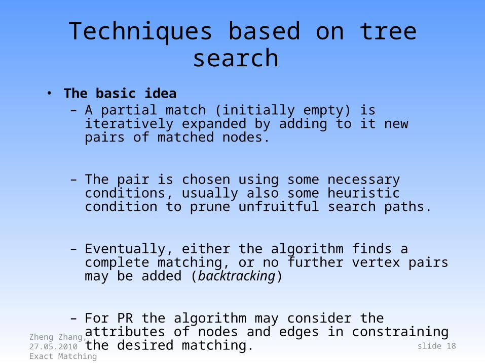
• The basic idea– A partial match (initially empty) is iteratively expanded by adding to
it new pairs of matched nodes.
– The pair is chosen using some necessary conditions, usually also some heuristic condition to prune unfruitful search paths.
– Eventually, either the algorithm finds a complete matching, or no further vertex pairs may be added (backtracking)
– For PR the algorithm may consider the attributes of nodes and edges in constraining the desired matching.

Zheng Zhang, 27.05.2010 Exact Matching slide 19
Techniques based on tree search
• The backtracking algorithm– depth-first search(DFS): it progresses by expanding the first child node of the search tree that
appears and thus going deeper and deeper until a goal node is found, or until it hits a node that has no children.
– Branch and bound(B&B): it is a BFS(breadth-first search)-like search for the optimal solution.
Branch is that a set of solution candidates is splitted into two or more smaller sets; bound is that a procedure upper and lower bounds.
10 11
12
1
2
3
4
6
7
5
8
9
11 12
8
1
2
5
9
6
3
10
4
7
Zheng Zhang, 27.05.2010 Exact Matching slide 20
Techniques based on tree search
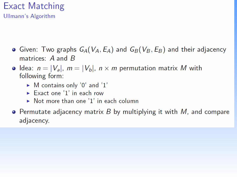
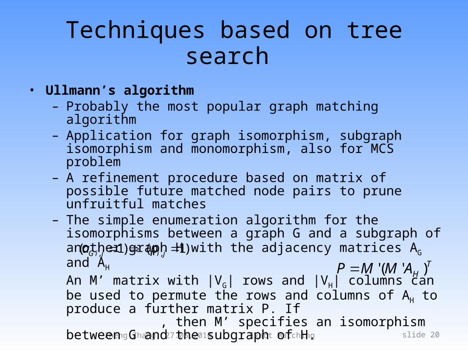
• Ullmann’s algorithm– Probably the most popular graph matching algorithm– Application for graph isomorphism, subgraph isomorphism and
monomorphism, also for MCS problem– A refinement procedure based on matrix of possible future matched
node pairs to prune unfruitful matches– The simple enumeration algorithm for the isomorphisms between a
graph G and a subgraph of another graph H with the adjacency matrices AG and AH
An M’ matrix with |VG| rows and |VH| columns can be used to permute the rows and columns of AH to produce a further matrix P. If , then M’ specifies an isomorphism between G and the subgraph of H.
[J.R.Ullmann.An algorithm for subgraph isomorphism.]
THAMMP )'('
)1()1( ,, jijiG pa

Zheng Zhang, 27.05.2010 Exact Matching slide 21
Techniques based on tree search
• Ullmann’s algorithm– Example for permutation matrix– The elements of M’ are 1’s and 0’s, such that each row contains 1 and
each column contains 0 or 1
3
1
2 4
2
1
3
H
4 )'(' MMP
011
100
100
100
100
011
100
.
0010
0100
0001
0010
0010
1101
0010
.
0010
0100
0001
0010
0100
0001
)'('T
THAMMP
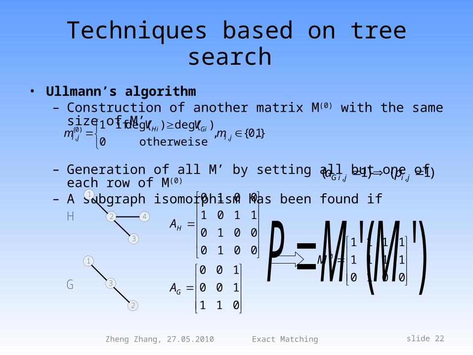
Zheng Zhang, 27.05.2010 Exact Matching slide 22
Techniques based on tree search
• Ullmann’s algorithm– Construction of another matrix M(0) with the same size of M’
– Generation of all M’ by setting all but one of each row of M(0)
– A subgraph isomorphism has been found if
)'(' MMP
}1,0{,otherweise0
)deg()deg(if1,
)0(,
jiGiHi
ji mVV
m
)1()1( ,, jijiG pa
3
1
2 4
2
1
3
H
G
011
100
100
0010
0010
1101
0010
G
H
A
A
0010
1111
11110M

Zheng Zhang, 27.05.2010 Exact Matching slide 23
Techniques based on tree search
• Ullmann’s algorithm– Example
)'(' MMP
0010
1111
1111
0010
1111
0001
0010
1111
0010
0010
1111
0100
0010
1111
1000
0010
0100
0001
0010
1000
0001
0010
0001
0100
0010
1000
0100
0010
0001
1000
0010
0100
1000
1
3
2
4 1
3
3
2 2
3
1
4 1
3
1
2
1
2
3
4
2
3
3
1 1
3
2
1
011
100
100
)'(' THAMMP
011
100
100
with compared GA
1
3
2

Zheng Zhang, 27.05.2010 Exact Matching slide 24
Techniques based on tree search
• Ghahraman’s algorithm– Application for monomorphism– Use of the netgraph obtained from the Cartesian product of the nodes
of two graph, monomorphisms correspond to particular subgraphs of the netgraph
– A strong necessary condition and a weak one, then two versions of the algorithm to detect unfruitful partial solutions
• VF and VF2 algorithm– Application for isomorphism and subgraph isomorphism– VF algorithm defines a heuristic based on the analysis of the sets of
nodes adjacent to the ones already considered in the partial mapping.– VF2 algorithm reduces the memory requirement from O(N2) to O(N).)'(' MMP

Zheng Zhang, 27.05.2010 Exact Matching slide 25
Techniques based on tree search
• Bron and Kerbosh’s algorithm– Application for the clique detection and the MCS problem– Based on the use of a heuristic for pruning the search tree– Simplicity and an acceptable performance in most cases
• Other algorithms for the MCS problem– Balas and Yu’s alogrithm also defines a heristic, but based on graph
colouring techniques.– McGregor’s alogrithm is not applicated for a maximum clique
problem.– Koch’s alogrithm is applicated for a slightly simplified version of the
MCS problem and suggests the use of the Bron and Kerbosh’s algorithm.

Zheng Zhang, 27.05.2010 Exact Matching slide 26
Other techniques
• Based on the A* algorithm– It uses a distance-plus-cost heuristic function to determine the order
in which the search visits nodes in the tree. The heuristic is a sum of two functions: the path-cost function, i.e. the cost from the starting node to the current node, and an admissible “heuristic estimate” of the distance to the goal.
– Demko’s algorithm investigates a generalization of MCS to hypergraphs.
• Based on group theory– McKay’s Nauty(No automorphisms yes?) algorithm deals only with the
isomorphism problem. It constructs the automorphism group of each of the input graphs and derives a canonical labeling. The isomorphism can be checked by verifying the equality of the adjacency matrices.

Zheng Zhang, 27.05.2010 Exact Matching slide 27
Conclusion
• The exact graph matching problem is of interest in a variety of different pattern recognition contexts.
• Of the exact graph matching problems, exact isomorphism is very seldom used in PR while subgraph isomorphism, monomorphism and the MCS problem are popularly proposed.
• Ullmann’ algorithm, VF2 algorithm and Nauty algorithm are mostly used algorithms, which based on the search methods, and may outperform others. Most modified algorithms adopt some conditions to prune the unfruitful partial matching.


)(
)()|()|(
yp
pypyp
Bayes for Beginners
)(
)()|()|(
yp
pypyp
)(
)()|()|(
yp
pypyp
Reverend Thomas Bayes (1702-61)
)(
)()|()|(
yp
pypyp
)(
)()|()|(
yp
pypyp
)(
)()|()|(
yp
pypyp
)(
)()|()|(
yp
pypyp

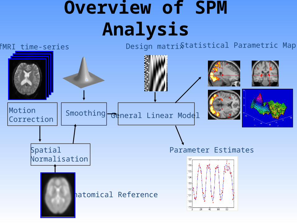
Overview of SPM Analysis
MotionCorrection
Smoothing
SpatialNormalisation
General Linear Model
Statistical Parametric MapfMRI time-series
Parameter Estimates
Design matrix
Anatomical Reference

Templateimage
Affine registration.(2 = 472.1)
Non-linearregistration
withoutBayes
constraints.(2 = 287.3)
Non-linearregistration
usingBayes.
(2 = 302.7)
Without Bayesian constraints, the non-linear spatial normalisation can introduce unnecessary warps.
Spatial Normalisation - Overfitting

Bayes and image segmentation• Want to automatically classify regions into grey matter, white matter, CSF and non-brain tissue.
• How do we use prior information? (probabilities of each voxel being of a particular type derived from a database of 152 scans)
•Bayes!
• Want to automatically classify regions into grey matter, white matter, CSF and non-brain tissue.
• How do we use prior information? (probabilities of each voxel being of a particular type derived from a database of 152 scans)
•Bayes!
A big advantage of a Bayesian approach
• Allows a principled approach to the exploitation of all available data …
• with an emphasis on continually updating one’s models as data accumulate
• as seen in the consideration of what is learned from a positive mammogram
Bayesian Reasoning
- Casscells, Schoenberger & Grayboys, 1978- Eddy, 1982- Gigerenzer & Hoffrage, 1995, 1999- Butterworth, 2001- Hoffrage, Lindsey, Hertwig & Gigerenzer, 2001
When PREVALENCE, SENSITIVITY, and FALSE POSITIVE RATES are given, most physicians misinterpret the information in a
way that could be potentially disastrous for the patient.

Bayesian Reasoning
ASSUMPTIONS1% of women aged forty who participate in a routine screening have breast cancer80% of women with breast cancer will get positive tests9.6% of women without breast cancer will also get positive tests
EVIDENCEA woman in this age group had a positive test in a routine screening
PROBLEMWhat’s the probability that she has breast cancer?

Bayesian Reasoning
ASSUMPTIONS10 out of 1000 women aged forty who participate in a routine screening have breast cancer800 out of 1000 of women with breast cancer will get positive tests95 out of 1000 women without breast cancer will also get positive tests
PROBLEMIf 1000 women in this age group undergo a routine screening, about what fraction of women with positive tests will actually have breast cancer?

Bayesian Reasoning
ASSUMPTIONS100 out of 10,000 women aged forty who participate in a routine screening have breast cancer80 of every 100 women with breast cancer will get positive tests950 out of 9,900 women without breast cancer will also get positive tests
PROBLEMIf 10,000 women in this age group undergo a routine screening, about what fraction of women with positive tests will actually have breast cancer?

Bayesian ReasoningBefore the screening:100 women with breast cancer9,900 women without breast cancer
After the screening:A = 80 women with breast cancer and positive testB = 20 women with breast cancer and negative testC = 950 women without breast cancer and positive
testD = 8,950 women without breast cancer and
negative test
Proportion of cancer patients with positive results, within the group of ALL patients with positive
results:A/(A+C) = 80/(80+950) = 80/1030 = 0.078 = 7.8%

Compact Formulation
C = cancer present, T = positive testp(A|B) = probability of A, given B, ~ = not
PRIOR PROBABILITYp(C) = 1%
CONDITIONAL PROBABILITIESp(T|C) = 80%
p(T|~C) = 9.6%
POSTERIOR PROBABILITY (or REVISED PROBABILITY)p(C|T) = ?
PRIORS

Bayesian ReasoningBefore the screening:100 women with breast cancer9,900 women without breast cancer
After the screening:A = 80 women with breast cancer and positive testB = 20 women with breast cancer and negative testC = 950 women without breast cancer and positive
testD = 8,950 women without breast cancer and
negative test
Proportion of cancer patients with positive results, within the group of ALL patients with positive
results:A/(A+C) = 80/(80+950) = 80/1030 = 0.078 = 7.8%

Bayesian ReasoningPrior Probabilities:
100/10,000 = 1/100 = 1% = p(C)
9,900/10,000 = 99/100 = 99% = p(~C)
Conditional Probabilities:
A = 80/10,000 = (80/100)*(1/100) = p(T|C)*p(C) = 0.008
B = 20/10,000 = (20/100)*(1/100) = p(~T|C)*p(C) = 0.002
C = 950/10,000 = (9.6/100)*(99/100) = p(T|~C)*p(~C) = 0.095
D = 8,950/10,000 = (90.4/100)*(99/100) = p(~T|~C) *p(~C) = 0.895
Rate of cancer patients with positive results, within the group of ALL patients with positive results:
A/(A+C) = 0.008/(0.008+0.095) = 0.008/0.103 = 0.078 = 7.8%


-----> Bayes’ theorem
p(T|C)*p(C)p(C|T) = ______________________
P(T|C)*p(C) + p(T|~C)*p(~C)
A
A + C

Comments
• Common mistake: to ignore the prior probability• The conditional probability slides the revised
probability in its direction but doesn’t replace the prior probability
• A NATURAL FREQUENCIES presentation is one in which the information about the prior probability is embedded in the conditional probabilities (the proportion of people using Bayesian reasoning rises to around half).
• Test sensitivity issue (or: “if two conditional probabilities are equal, the revised probability equals the prior probability”)
• Where do the priors come from?
-----> Bayes’ theorem
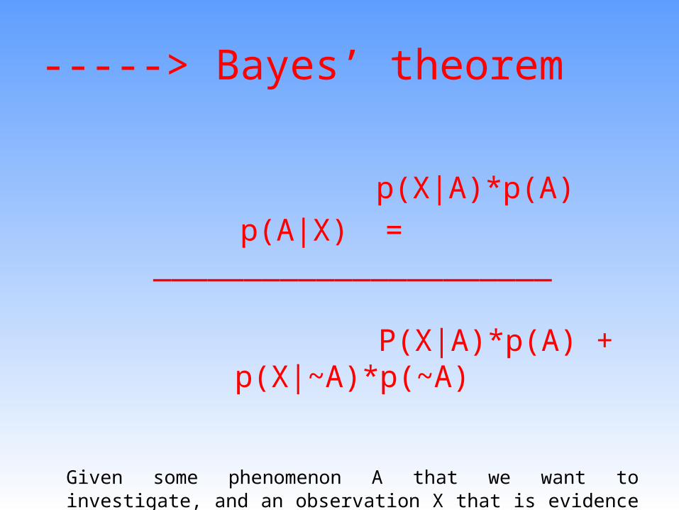
p(X|A)*p(A)p(A|X) = ______________________
P(X|A)*p(A) + p(X|~A)*p(~A)
Given some phenomenon A that we want to investigate, and an observation X that is evidence about A, we can update the original probability of A, given the new evidence X.

It relates the conditional density of a parameter (posterior probability) with its unconditional density (prior, since depends on information present before the experiment).
The likelihood is the probability of the data given the parameter and represents the data now available.
Bayes’ Theorem for a given parameter
p (data) = p (data) p () / p (data)
1/P (data) is basically a normalizing constant
Posterior likelihood x prior
The prior is the probability of the parameter and represents what was thought before seeing the data.
The posterior represents what is thought given both prior information and the data just seen.

Likelihood: p(y|) = N(Md, ld-1)
Prior: p() = N(Mp, lp-1)
Posterior: p(|y) ∝ p(y|)* p() = N(Mpost, lpost-1)
Mp
lp-1
Mpost
lpost-1
ld-1
Md
lpost = ld + lp Mpost = ld Md + lp Mp
lpost
Posterior Probability Distributionprecision = 1/2

Activations in fMRI….
• Classical – ‘What is the likelihood of getting these data
given no activation occurred?’
• Bayesian option (SPM2)– ‘What is the chance of getting these parameters,
given these data?

What use is Bayes in deciding what brain regions are active in a particular study?
• Problems with classical frequentist approach– All inferences relate to disproving the null hypothesis– Never fully reject H0, only say that the effect you see is
unlikely to occur by chance– Corrections for multiple comparisons
• significance depends on the number of contrasts you look at– Very small effects can be declared significant with enough
data• Bayesian Inference offers a solution through Posterior
Probability Maps (PPMs)
SPMs and PPMsSP
Mmip
[0, 0
, 0]
<
< <
PPM2.06
rest [2.06]
SPMresults:C:\home\spm\analysis_PET
Height threshold P = 0.95
Extent threshold k = 0 voxels
Design matrix1 4 7 10 13 16 19 22
147
1013161922252831343740434649525560
contrast(s)
4
SPMmip
[0, 0
, 0]
<
< <
SPM{T39.0
}
rest
SPMresults:C:\home\spm\analysis_PET
Height threshold T = 5.50
Extent threshold k = 0 voxels
Design matrix1 4 7 10 13 16 19 22
147
1013161922252831343740434649525560
contrast(s)
3
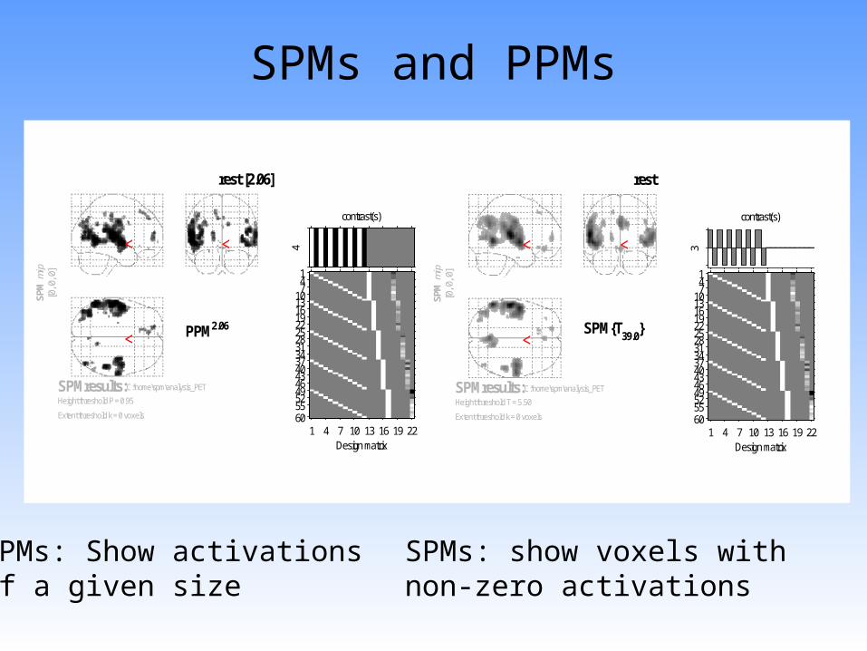
PPMs: Show activationsof a given size
SPMs: show voxels with non-zero activations

PPMs
Advantages Disadvantages
One can infer a causeDID NOT elicit a response
SPMs conflate effect-size and effect-variability
Computationally demanding (priors are determined empirically)
Utility of Bayesian approach is yetto be established

Frequentist vs. Bayesian by Berry
1. Probabilities of data vs. probabilities of parameters (& also data).
2. Evidence used:– Frequentist measures specific to experiment.– Posterior distribution depends on all available
information.Makes Bayesian approach appealing, but assembling, assessing, & quantifying information is work.

3. Depend on probabilities of results that could occur vs. did occur:– Frequentist measures (e.g., p values, confidence intervals)
incorporate probabilities of data that were possible but did not occur.
– Posterior depends on data only through the likelihood, which is calculated from observed data.
4. Flexibility:– Frequentist measures depend on design; require that
design be followed.– Bayesian view: update continually as data accumulate
(only requirement is honesty). Sample size: need not choose in advance. Weigh costs/benefits; decide whether to start experiment. After experiment starts, decide whether to continue—stop at any time, for any reason.

5. Decision making– Frequentist: historically avoided.– Bayesian: tailored to decision analysis; losses and
gains considered explicitly.

• Statistics: A Bayesian Perspective D. Berry, 1996, Duxbury Press.– excellent introductory textbook, if you really want to understand what it’s all about.
• http://ftp.isds.duke.edu/WorkingPapers/97-21.ps– “Using a Bayesian Approach in Medical Device Development”, also by Berry
• http://www.pnl.gov/bayesian/Berry/– a powerpoint presentation by Berry
• http://yudkowsky.net/bayes/bayes.html– Extremely clear presentation of the mammography example; highly polemical and fun
too!• http://www.stat.ucla.edu/history/essay.pdf
– Bayes’ original essay• Jaynes, E. T., 1956, `Probability Theory in Science and Engineering,' (No. 4 in
`Colloquium Lectures in Pure and Applied Science,' Socony-Mobil Oil Co. USA. http://bayes.wustl.edu/etj/articles/mobil.pdf– A physicist’s take on Bayesian approaches. Proposes an interesting metric of probability
using decibels (yes, the unit used for sound levels!).• http://www.sportsci.org/resource/stats/
– a skeptical account of Bayesian approaches. The rest of the site is very informative and sensible about basic statistical issues.
References

Bayes’ ending
)(
)()|()|(
yp
pypyp
)(
)()|()|(
yp
pypyp
)(
)()|()|(
yp
pypyp
)(
)()|()|(
yp
pypyp
)(
)()|()|(
yp
pypyp
)(
)()|()|(
yp
pypyp
)(
)()|()|(
yp
pypyp
Bunhill Fields Burial Groundoff City Road, EC1