1

Zebrafish Illumina Data Analysis Protocol

Accompanying the publication:

Efficient Mapping and Cloning of Mutations in Zebrafish by Low

Coverage Whole Genome Sequencing

Margot E. Bowen & Katrin Henke, Kellee Siegfried-Harris, Matthew L. Warman, Matthew P. Harris.

Genetics, 2012

Described in this protocol are the steps required for the analysis of low coverage Illumina whole genome sequence data from a pool of F2 mutants. This protocol utilizes whole genome sequence data from the Tü, WK, TLF and AB laboratory strains to: (1) facilitate the accurate identification of common polymorphisms present in a mutant pool, which can be used for homozygosity mapping; (2) identify the likely parental origin of alleles in a mutant pool, which can be used for mapping based on strain specific signatures; (3) within the linked interval, distinguish common polymorphisms from variants unique to the mutant pool, which will be candidates for the causative mutation. Contents

1. Software requirements……………………………………………….. 2 2. Downloading datasets………………………………………………… 2 3. Command line usage…………………………………………………. 3 4. Preparing the reference genome……………………………………. 3 5. Alignment of reads to the reference genome……………………… 4 6. Preparing BAM files……………………………………….………….. 5 7. Variant calling…………………………………………………………. 6 8. Rough Mapping……………………………………………………….. 7 9. Narrowing down the linked interval…………………………………. 8 10. Identifying candidate mutations…………………………………….. 10 11. Identifying candidate causative mutations in regions covered by only one read……..………………………… 11 12. Identifying candidate causative mutations: indels………………… 12 13. Appendix 1: visualizing the data used for calculating the mapping score…………………………………… 13

2

1. Software requirements The following publically available software should be installed:

1. Any suitable alignment software, such as Novoalign (http://www.novocraft.com/). 2. SAMtools (http://samtools.sourceforge.net/). 3. Picard (http://sourceforge.net/projects/picard/) 4. Genome Analysis Toolkit (GATK)

(http://www.broadinstitute.org/gsa/wiki/index.php/The_Genome_Analysis_Toolkit) 5. Integrative Genomics Viewer (IGV) (http://www.broadinstitute.org/igv/) 6. Annovar (http://www.openbioinformatics.org/annovar/)

2. Downloading datasets The following datasets should be downloaded from http://fishyskeleton.com/:

1. Whole genome sequence data for six reference strain pools

Folder name: aligned_sequences Example file name: TLF_chr1.bam, TLF_chr1.bam.bai

Illumina sequencing reads (100bp single end), for the Tü, WIK, AB, TLF laboratory strains, aligned to the zebrafish reference genome (Zv9/danRer7). For the Tü and WIK strains, sequencing was performed separately on fish maintained in Tübingen, Germany (referred to as TUG and WKG) and fish maintained at Children’s Hospital, Boston (referred to as TUB and WKB). Each aligned sequence file (in the BAM file format) is paired with an index file (.bai).

2. Coordinates of repetitive sequences

Folder name: repeat_mask Example file name: danRer7_repeatmask_chr1.bed Coordinates of all interspersed repeats and low complexity sequences in the zebrafish genome. This is the output of the RepeatMasker (http://www.repeatmasker.org/) that has been converted to the BED file format.

3. Physical coordinates of cM intervals Folder name: MGH_map Example file name: chr1_cM Estimated coordinates for each 0.25 cM interval in the genome. These estimates are based on the genetic distance of markers in the MGH meiotic map (http://zfin.org/zf_info/downloads.html#map) that have been mapped to the zv9 reference genome.

3

4. Zebrafish genes and dbSNPs

Folder name: zebradb Example file name: danRer7_ensGene.txt Coordinates and sequences of Ensembl and Refseq zebrafish genes (http://hgdownload.cse.ucsc.edu/goldenPath/danRer7/database/) and dbSNPs (http://useast.ensembl.org/info/data/ftp/index.html) that have been formatted for use in the Annovar software.

5. Coding exon bases Folder name: coding_exon_bases Example file name: coding_bases_chr1 The genomic coordinate of each coding exon base as well as bases up to 15 bp upstream and downstream of each coding exon. This list was constructed from the merged dataset of all Refseq and Ensemble coding exons.

6. Perl scripts

Folder name: perl Example file name: mapping_score.pl Perl scripts used for mapping and candidate mutation identification.

3. Command line usage Since it is often required to run the same command on multiple files, wild cards and for loops are used in this protocol. The wild card symbol “*” can be used to represent any character or characters in a file name, while the wild card symbol “?” can be used to represent any single character in a file name. For Loops can, for example, be used to run the same command on files from all 25 chromosomes (for f in {1..25} ; do echo $f ; command chr"$f" ; done). Users unfamiliar with these concepts are encouraged to consult an introductory Unix text. 4. Preparing the reference genome Some programs, such as the GATK, require the reference genome to have the .fasta extension, and that a .dict dictionary file and a .fai fasta index file are present in the same folder as the reference genome. See the GATK website for more details: http://www.broadinstitute.org/gsa/wiki/index.php/Preparing_the_essential_GATK_input_files:_the_reference_genome

4

1. Download the zebrafish genome sequence

The zebrafish genome sequence, danRer7.fa, can be downloaded from the UCSC Genome Bioinformatics site (http://hgdownload.cse.ucsc.edu/goldenPath/danRer7/bigZips/).

2. Rename the reference genome to .fasta mv danRer7.fa danRer7.fasta

3. Create a fasta sequence dictionary file, using the CreateSequenceDictionary.jar file from Picard

java -jar CreateSequenceDictionary.jar R=danRer7.fasta O=danRer7.dict

4. Create a fasta index file (.fai) using SAMtools samtools faidx danRer6.fasta 5. Aligning reads to the reference genome Alignment can be performed using any suitable alignment software. As an example, the commands for Novoalign are provided:

1. Prepare the reference genome for use in Novoalign: novoindex danRer7_novoindex danRer7.fasta

2. To speed up the alignment, the input file can first be split into multiple smaller files split -l 5000000 sequence.txt splitsequence_ This splits up the input fastq file (sequence.txt) into files each containing 5 million lines (1.25 million reads) that are named splitsequence_aa, splitsequence _ab, splitsequence _ac etc.

3. Align the reads to the reference genome using Novoalign for f in splitsequence_* ; do echo $f ; novoalign -f $f -d danRer7.fa_novoindex -o SAM -F ILMFQ -a AGATCGGAAGAGCGGTTCAGCAGGAATGCCGAGACCGATCTCGTATGCCGTCTTCTGCTTG > "$f".sam 3’ adaptor trimming (-a) is necessary if it is expected that a significant fraction of library fragments will have an insert size less than the Illumina read length. For example, libraries prepared from degraded genomic DNA in our laboratory had a significant fraction of fragments with an insert size below 100bp. When Illumina 100bp sequencing is performed on these fragments, the 3’ end of some reads will correspond to the adaptor sequence, which should be removed before alignment to the reference genome. The sequence listed above is the sequence corresponding to the Illumina paired end adaptor used in our laboratory (which can be used for both paired and single end sequencing).

5

6. Preparing BAM files

1. Convert SAM files to BAM files for f in splitsequence_*.sam ; do echo $f ; samtools import danRer7.fasta $f "$f".bam ; done

2. Sort reads based on their location in the genome for f in splitsequence_*.sam.bam ; do echo $f ; samtools sort $f "$f".sort ; done

3. Merge multiple BAM files samtools merge -rh readgroup.txt merge_mutant1.bam splitsequence_*.sam.bam.sort.bam For each read, a read group tag will be added which will specify which input file contained that read. Some programs, such as the GATK, require that all reads contain a read group tag. The readgroup.txt file must first be created as a text file. It should contain one line for each input file. Shown here are the first three lines: @RG ID:splitsequence_aa.sort SM:mutant1 LB:mutant1 PL:Illumina @RG ID:splitsequence_ab.sort SM:mutant1 LB:mutant1 PL:Illumina @RG ID:splitsequence_ac.sort SM:mutant1 LB:mutant1 PL:Illumina The ID tag must contain the input file name (excluding the .bam extension) The SM tag must contain the name of the sample (for example mutant1) The LB tag lists the name of the library. If only one library was made for each mutant, the library name will be the same as the sample name. The PL tag contains the name of the sequencing platform.

4. Index the merged BAM file samtools index merge_mutant1.bam

5. Remove PCR duplicates java -jar picard-tools/MarkDuplicates.jar I= merge_mutant1.bam O= merge_mutant1.PCR.bam METRICS_FILE= merge_mutant1_PCRmetrics ASSUME_SORTED=TRUE REMOVE_DUPLICATES=true

6. Index the merged PCR duplicate removed file samtools index merge_mutant1.PCR.bam

7. Create a file for each chromosome for f in {1..25} ; do echo $f ; samtools view -b merge_mutant1.PCR.bam chr"$f" -o mutant1_chr"$f".bam ; done To decrease the computational load, downstream analyses are performed on one chromosome at a time.

6

8. Index the BAM file for each chromosome

samtools index mutant1_chr*.bam

9. Determine the depth of coverage for each chromosome for f in {1..25} ; do echo $f ; java -jar GenomeAnalysisTK.jar -T DepthOfCoverage -R danRer7.fasta -I mutant1_chr"$f".bam -o depth_mutant1_chr"$f" -L chr"$f" --omitDepthOutputAtEachBase ; done 7. Variant calling

1. Perform variant calling on all mutants and reference strains simultaneously for f in {1..25} ; do echo $f ; samtools mpileup -ugf danRer7.fasta *_chr"$f".bam | samtools/bcftools view -vcg - > chr"$f".vcf ; done The BAM files for each chromosome for the reference strains must first be downloaded from http://fishyskeleton.com/ and stored in the same folder as the BAM files for your mutant. For example, for chromosome 1, variant calling will be performed on the BAM file(s) for your mutant(s), (mutant1_chr1.bam, mutant2_chr1.bam etc) as well as the reference strains (AB_chr1.bam, TLF_chr1.bam, TUB_ch1.bam, TUG_chr1.bam, WKB_chr1.bam, WKG_chr1.bam). Performing variant calling on all samples simultaneously increases the accuracy of variant calling on low coverage sequence data, and is also necessary for downstream analyses of the parental origin of SNPs used for calculating the mapping score.

2. Change the header to make the variant file compatible with GATK for f in chr*.vcf ; do echo $f ; sed 's/##fileformat=VCFv4.1/##fileformat=VCFv4.0/g' $f > "$f"_header ; done

3. Separate the indels from the SNPs for f in chr*vcf_header ; do echo $f ; grep -v INDEL $f > "$f"_noINDEL; done for f in chr*vcf_header ; do echo $f ; grep INDEL $f > "$f"_INDEL ; done

Due to the inaccuracy of aligning reads with insertions or deletions, only SNPs, and not indels, are used for mapping purposes. However, once the linked interval is identified, indels can then be analyzed to identify indels, as well as SNPs, unique to a mutant pool, which will be candidates for the causative mutation.

4. Identify higher quality SNPs

for f in {1..25} ; do echo $f ; java -jar GenomeAnalysisTK.jar -T VariantFiltration -R danRer7.fasta -B:variant,VCF chr"$f".vcf_header_noINDEL -o chr"$f".vcf_noINDEL_filtered -B:mask,Bed repeatmask/danRer7_repeatmask_chr"$f".bed --maskName RepeatMask --clusterWindowSize 10 --filterExpression "QUAL < 30" --filterName "QualFilter" --filterExpression "DP < 8" --filterName "LowDepth" --filterExpression "DP > 60" --filterName "HighDepth" --filterExpression "MQ < 40" --filterName "MapQual" ; done

7

Due to the frequent misalignment of reads containing repetitive sequences, SNPs lying in interspersed repeats or low complexity sequences are excluded from the analysis. The BED files of repeat masked sequences can be downloaded from http://fishyskeleton.com/. The filtering criteria can be adjusted as needed. See http://www.broadinstitute.org/gsa/wiki/index.php/VariantFiltrationWalker for details on the parameters used for filtering. 8. Rough mapping To identify regions of homozygosity-by-descent, a Mapping Score is calculated in sliding windows of 20 cM in size. This Mapping Score is designed to identify regions that have both a reduction in the number of heterogeneous SNPs and a reduction in the number of alleles inherited from the mapping strain. Mapping score = (homogeneous sites) X (reference genome alleles) (heterogeneous sites) (mapping strain alleles)

1. Identify SNPs useful for mapping for f in chr*.vcf_noINDEL_filtered; do echo $f ; perl ./perl/classifySNPs.pl $f mutant1 TU WK > "$f"_mutant1_TU_WK.cn ; done This program creates three output files for each chromosome, for example: chr1.vcf_noINDEL_filtered_mutant1_TU_WK.cn This file is used for calculating the mapping score (see below) and narrowing down the linked interval (see section 9) chr1.vcf_noINDEL_filtered_mutant1_homnovelSNPs This file contains homogeneous SNPs, unique to the mutant pool, that will be used for identifying candidate causative mutations (see section 10). chr1.vcf_noINDEL_filtered_mutant1_hetSNPs This file lists the coordinates and quality scores (in the SAMtools/BCFtools output format) of all SNPs classified as heterogeneous in the mutant pool.

2. Convert physical coordinates to cM coordinates for f in {1..25} ; do echo $f ; perl ./perl/convert_bp_to_cM.pl ./MGH_map/chr"$f"_cM chr"$f".vcf_noINDEL_filtered_mutant1_TU_WK.cn > chr"$f"_mutant1_TU_WK_cM.cn ; done The MGH_map folder must first be downloaded from http://fishyskeleton.com/.

3. Calculate the mapping score for f in {1..25} ; do echo $f ; perl ./perl/mapping_score.pl chr"$f"_mutant1_TU_WK_cM.cn 20 > chr"$f"_mutant1_TU_WK_mappingscore_20cM ; done We recommend using a window size of 20 cM. If necessary, a different window size can be specified by the number after the file name.

8

4. Combine the mapping score for each chromosome, in the correct order: cat chr1_mutant1_TU_WK*20cM chr2_mutant1_TU_WK*20cM chr3_mutant1_TU_WK*20cM chr4_mutant1_TU_WK*20cM chr5_mutant1_TU_WK*20cM chr6_mutant1_TU_WK*20cM chr7_mutant1_TU_WK*20cM chr8_mutant1_TU_WK*20cM chr9_mutant1_TU_WK*20cM chr10_mutant1_TU_WK*20cM chr11_mutant1_TU_WK*20cM chr12_mutant1_TU_WK*20cM chr13_mutant1_TU_WK*20cM chr14_mutant1_TU_WK*20cM chr15_mutant1_TU_WK*20cM chr16_mutant1_TU_WK*20cM chr17_mutant1_TU_WK*20cM chr18_mutant1_TU_WK*20cM chr19_mutant1_TU_WK*20cM chr20_mutant1_TU_WK*20cM chr21_mutant1_TU_WK*20cM chr22_mutant1_TU_WK*20cM chr23_mutant1_TU_WK*20cM chr24_mutant1_TU_WK*20cM chr25_mutant1_TU_WK*20cM > mutant1_TU_WK_mappingscore20cMall The mapping score file contains the following data:

Column 1: chromosome number Column 2: genomic coordinate (in bp) of the start of the window Column 4: mapping score Column 5: ratio of homogeneous to heterogeneous SNPs Column 6: ratio of reference alleles to mapping strain alleles

Any suitable graphing software can be used to create plots to visualize the mapping score across the genome. Regions with high mapping scores are candidates for the linked region. In our analyses, linked regions all had a mapping score greater than 100. However, the actual mapping score will depend on the location of the recombination events with respect to the causative mutation, and the accuracy of the MGH meiotic map in that region. Some regions with a very high recombination rate (eg. telomeric regions of chr21) are prone to false positive high mapping scores. This is because, since these regions of high recombination span a very small physical distance, the total number of SNPs in these regions is low, and therefore slight variation in, for example, the number of heterogeneous SNPs, can have a large effect on the mapping score. To visualize the data used to calculate the mapping score, see Appendix 1. 9. Narrowing down the linked region Once linkage to a broad window has been confirmed, the boundaries of the smaller region of homogeneity can be defined. To visualize the number of heterogeneous SNPs across the linked interval, the .cn files (section 8 step 1) can be visualized in IGV.

1. Open IGV and select “Zebrafish (Zv9/danRer7)” from the menu in the top left corner

2. Load the .cn file for the chromosome of interest.

File >> load from file >> select the .cn file of interest, for example: chr1.vcf_noINDEL_filtered_mutant1_TU_WK.cn

3. Select a chromosome number from the menu in the top left corner.

4. Convert heatmaps to line plots

9

In IGV, the default setting for this type of graph is a heatmap. Right click on the file names. A pop up menu will appear. Under “Type of Graph” select “Line Plot”.

5. Change track height if desired Right click on the track name, and under “Track Settings” select “Change Track Height” and type in a larger value.

6. Narrow down the interval by identifying the region of homogeneity Seven tracks are present for each .cn file. The first tracked is named mutant1het and represents the number of heterogeneous SNPs per bin size of 20,000 bp. This track is used to narrow down the interval. A region of homogeneity will appear as a region with only a very low number of heterogeneous SNPs that may be due to sequencing errors or alignment artifacts. Note: The six additional tracks are provided as extra information for users who are interested in seeing the data that was used to calculate the mapping score. These tracks are described in Appendix 1. Example for mutant sump: An IGV screen shot of the track showing the number of heterogeneous SNPs is shown for the mutant sump (described in our accompanying paper). For this mutant, a high mapping score was obtained on chromosome 16, from 35 Mb to 55 Mb. Linkage was confirmed to an SSLP marker located at 43.9 Mb on this chromosome. The name “NC31” was used for this mutant in our data analysis steps. Entire chromosome 16 for mutant NC31:

Note that the region of reduced heterogeneity spans from ~35 Mb to 55 Mb, which corresponds to the region that had a high mapping score. The additional region of reduced heterogeneity observed at ~18-25Mb would not be considered a candidate linked region, since it spans less than a few cM. Zoom in to the linked region by double clicking on the region of interest:

It can now be seen that the candidate region of homogeneity is ~42.4-50.2 Mb.

10

10. Identifying candidate causative mutations Once the linked interval has been identified, novel homogeneous SNPs lying in the linked region are selected as candidates for the causative mutation, and these are classifed as nonsynonymous, synonymous or noncoding.

1. Select unique homogeneous SNPs lying in linked interval For example, if the linked interval is identified as chr16:42000000-51000000: awk '($2 >= 42000000)&&($2 <= 51000000)' chr16.vcf_noINDEL_filtered_mutant1_homnovelSNPs > mutant1_homnovelSNPs_linked The chr16.vcf_noINDEL_filtered_mutant1_homnovelSNPs file was generated as the output of step 8-1. Each line in this file contains a homogeneous SNP that is unique to mutant1. Example of a SNP from this file: chr16 43278095 . C T 47.10 PASS AF1=0.1677;CI95=0.07143,0.2857;DP=42;DP4=17,16,8,1;FQ=47.9;MQ=60;PV4=0.06,3.5e-27,1,0.46 GT:PL:GQ 0/0:0,15,158:19 1/1:98,27,0:17 0/0:0,0,0:5 0/0:0,24,226:28 0/0:0,21,208:25 0/0:0,24,224:28 0/0:0,15,165:19 This format is described at http://samtools.sourceforge.net/mpileup.shtml. The order of the samples can be found in the last line of the header of the original vcf file. For example, mutant NC31 is the second sample:

#CHROM POS ID REF ALT QUAL FILTER INFO FORMAT AB NC31 … … TLF TUB TUG WKB WKG

2. Prepare the SNP file for Annovar

annovar/convert2annovar.pl -format vcf4 mutant1_homnovelSNPs_linked > mutant1_homnovelSNPs_linked_annovar

3. Filter out dbSNPs perl annovar/annotate_variation.pl -filter --genericdbfile danRer7_dbSNPs.txt --buildver danRer7 --dbtype generic mutant1_homnovelSNPs_linked_annovar annovar/zebradb The zebradb folder, downloaded from http://fishyskeleton.com/, should be stored in the annovar folder. Two files will be created: mutant1_homnovelSNPs_linked_annovar.danRer7_generic_dropped mutant1_homnovelSNPs_linked_annovar.danRer7_generic_filtered The dropped file contains SNPs that were listed in dbSNP. The filtered file contains SNPs that were not present in dbSNP.

4. Classify SNPs as synonymous, nonsynonymous or noncoding

11

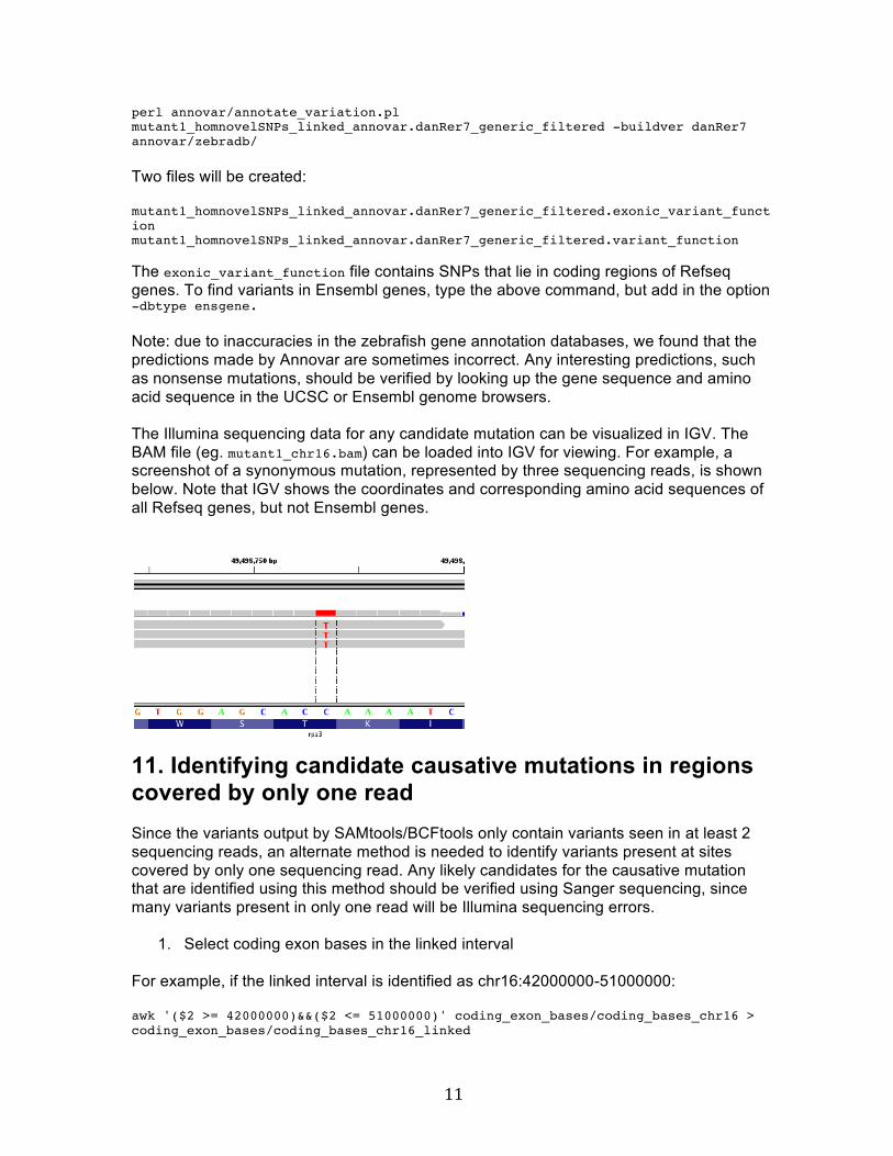
perl annovar/annotate_variation.pl mutant1_homnovelSNPs_linked_annovar.danRer7_generic_filtered -buildver danRer7 annovar/zebradb/ Two files will be created: mutant1_homnovelSNPs_linked_annovar.danRer7_generic_filtered.exonic_variant_function mutant1_homnovelSNPs_linked_annovar.danRer7_generic_filtered.variant_function The exonic_variant_function file contains SNPs that lie in coding regions of Refseq genes. To find variants in Ensembl genes, type the above command, but add in the option -dbtype ensgene. Note: due to inaccuracies in the zebrafish gene annotation databases, we found that the predictions made by Annovar are sometimes incorrect. Any interesting predictions, such as nonsense mutations, should be verified by looking up the gene sequence and amino acid sequence in the UCSC or Ensembl genome browsers. The Illumina sequencing data for any candidate mutation can be visualized in IGV. The BAM file (eg. mutant1_chr16.bam) can be loaded into IGV for viewing. For example, a screenshot of a synonymous mutation, represented by three sequencing reads, is shown below. Note that IGV shows the coordinates and corresponding amino acid sequences of all Refseq genes, but not Ensembl genes.

11. Identifying candidate causative mutations in regions covered by only one read Since the variants output by SAMtools/BCFtools only contain variants seen in at least 2 sequencing reads, an alternate method is needed to identify variants present at sites covered by only one sequencing read. Any likely candidates for the causative mutation that are identified using this method should be verified using Sanger sequencing, since many variants present in only one read will be Illumina sequencing errors.

1. Select coding exon bases in the linked interval For example, if the linked interval is identified as chr16:42000000-51000000: awk '($2 >= 42000000)&&($2 <= 51000000)' coding_exon_bases/coding_bases_chr16 > coding_exon_bases/coding_bases_chr16_linked

12

The coding_exon_bases folder should be downloaded from http://fishyskeleton.com/. These files contain a list of all coding exon bases as well as 15 bp of sequence flanking each exon (for the identification of splice site variants).

2. Generate a pileup for every coding exon base

samtools mpileup -l coding_exon_bases/coding_bases_chr16_linked -f danRer7.fasta -I *_chr16.bam > mpileup_codingexons_chr16_linked This lists the base pairs observed in each mutant and reference strain at each coding exon base. The BAM files for all reference strains and mutants must be stored in the same folder.

3. Indentify homogeneous mutations unique to a mutant pool perl perl/novelSNPs_oneread.pl mpileup_codingexons_chr16_linked 2 7 > mutant1_chr16_linked_homnovel_oneread This script requires three input values. Firstly, the name of the pileup file. Secondly, the number that to corresponds to the mutant pool when all samples are listed in alphabetical order. Thirdly, the total number of fish. For example, if one mutant (named mutant1) and the six reference pools were used for the pileup, the total number of fish is 7. The number corresponding to mutant1 will be 2, since the alphabetical order of the samples is AB, mutant1, TLF, TUB, TUG, WKB, WKG. The output file lists all homogeneous mutations unique to the mutant pool. This will include mutations at sites covered by only one read, as well as at sites covered by more than one read. For details on the pileup file format, please consult SAMtools documentation.

4. Filter out dbSNPs and classify SNPs as coding or noncoding Follow steps 10-3 and 10-4. The output file from the above command (mutant1_chr16_linked_homnovel_oneread) is already formatted for use in Annovar, so step 10-2 is not necessary. 12. Identifying candidate causative mutations: indels

1. Select indels in the linked interval

For example, if the linked interval is identified as chr16:42000000-51000000: awk '($2 >= 42000000)&&($2 <= 51000000)' chr16.vcf_INDEL > chr16.vcf_INDEL_linked The chr16.vcf_INDEL file was generated during step 7-3.

2. Identify homogeneous novel indels in the mutant pool perl perl/novelINDELS.pl chr16.vcf_INDEL_linked 2 > mutant1_hom_novel_INDEL_linked

13

The number corresponding to the mutant should be entered after the input file name (see section 11-3).

3. Classify indels as noncoding, frameshift, or non-frameshift Use Annovar, following step 10-2 to 10-4.

14

Appendix 1: visualizing the data used for calculating the mapping score Seven tracks are present in the .cn file that can be visualized in IGV (see section 9). These tracks represent data that is used for calculating the mapping score. IGV screen shot of chr16 for mutant NC31 (which maps to chr16:43.6Mb):

(note: the colors of the tracks were changed by right clicking on the track name, then selecting or “Change Track Color (Positive Values)”.) Description of each track: Track name Description* NC31het Heterogeneous (ie. both the reference allele and the

alternate allele are observed at a SNP site)

NC31hom_refornonref Homogeneous for either the reference or non-reference allele

NC31hom_nonref Homogeneous for the non-reference allele

TUSNP_sharedNC31 TUSNP_notsharedNC31

Tü SNPs were classified as non-reference alleles found in Tü (in either a homogeneous or heterogeneous state) but not in WIK. If at least one read representing the non-reference allele was also found in NC31, the Tü SNP was classified as being shared with NC31. If only reference genome alleles were found in NC31, the Tü SNP was classified as not shared with NC31.

WKSNP_sharedNC31 WKSNP_notsharedNC31

Same as above, but for non-reference alleles found in WIK but not Tü.

15

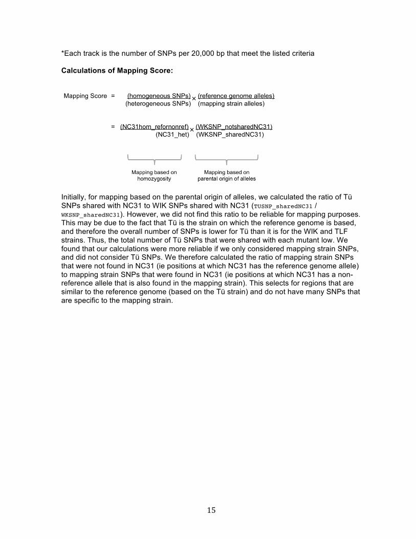
*Each track is the number of SNPs per 20,000 bp that meet the listed criteria Calculations of Mapping Score:

Initially, for mapping based on the parental origin of alleles, we calculated the ratio of Tü SNPs shared with NC31 to WIK SNPs shared with NC31 (TUSNP_sharedNC31 / WKSNP_sharedNC31). However, we did not find this ratio to be reliable for mapping purposes. This may be due to the fact that Tü is the strain on which the reference genome is based, and therefore the overall number of SNPs is lower for Tü than it is for the WIK and TLF strains. Thus, the total number of Tü SNPs that were shared with each mutant low. We found that our calculations were more reliable if we only considered mapping strain SNPs, and did not consider Tü SNPs. We therefore calculated the ratio of mapping strain SNPs that were not found in NC31 (ie positions at which NC31 has the reference genome allele) to mapping strain SNPs that were found in NC31 (ie positions at which NC31 has a non-reference allele that is also found in the mapping strain). This selects for regions that are similar to the reference genome (based on the Tü strain) and do not have many SNPs that are specific to the mapping strain.