Yield Curve Modelling with Skews and Stochastic Volatility

by

Leif Andersen and Jesper Andreasen

Bank of America Securities

April 2002 Modified August 2002

Abstract

This paper discusses a variety of techniques for modeling the evolution of interest rates in the presence of stochastic volatily. We cover both Libor Market models and low-dimensional Markovian HJM models. To facilitate model calibration, special emphasis is put on efficient pricing of plain-vanilla instruments. Effects of stochastic volatility on CMS structures as well as Bermudan swaptions are discussed.

2

1. Introduction.

There is currently great interest in improving fixed income models to better capture observed volatility skews and smiles in cap and swaption markets. Approaches suggested in the literature include state-dependent diffusions (see e.g. Andersen and Andreasen, 2000) and geometric Brownian motion overlaid with a jump process (as in Glasserman and Kou, 1999). While these approaches are both reasonable, they are not without problems and it is unlikely that they tell the whole story. For instance, as discussed in Rebonato (2001) and in a number of empirical studies, inclusion of stochastic volatility into fixed income models can significantly improve the realism of the models. This paper continues this line of research by focusing on flexible, yet practical techniques for the financial engineer to construct interest rate models with stochastic volatility. We work with both multi-factor Libor Market (LM) models and low-dimensional Markovian HJM models, and demonstrate that the proposed models are reasonable from an empirical perspective. To aid calibration and fast mark-to-market of simple derivatives, we pay particular attention to the development a variety of exact and approximative techniques to compute the prices of basic European derivatives such as caps, swaptions, and CMS options. Further, the paper introduces numerical methods for complex derivatives and gives examples of the effects of stochastic volatility on Bermudan swaptions. 2. Notation. Libor Market model.

Let 1 Ni iT = be a discrete tenor structure and let ( )kF t denote the time t value of the

discretely compounded forward rate spanning 1[ , ]k kT T + . Also, let , ( )s eR t denote the par rate of a plain-vanilla swap exchanging fixed for floating payments at points in the tenor structure 1 2, ,...,s s eT T T+ + . With 1i i iT Tδ +≡ − and ( , )P t T being the time t discount factor to time T, we have

( )11( ) ( , ) / ( , ) 1 , ;k k k k kF t P t T P t T t Tδ −

+= − ≤

, , 11,

( , ) ( , )( ) , ( ) ( , ), .( )

ee s

s e s e i i si ss e

P t T P t TR t A t P t T t TA t

δ −= +

−= = ≤∑

We now postulate model arbitrage-free forward rate dynamics of the form

( ) T( ) ( ) ( ) ( ) ( ) ( ) ( )k k k kdF t F t V t t V t t dt dW tϕ λ µ = + (1a)

where W is an n-dimensional Brownian motion, :ϕ + +→¡ ¡ is a well-behaved deterministic function satisfying (0) 0ϕ = , kλ is an n-dimensional deterministic volatility function loading each scalar Brownian motion, ( )V t is a scalar positive process to be specified, and kµ is an n-dimensional numeraire-specific drift that ensures lack of arbitrage across bonds. An expression for kµ can be found in Andersen and Andreasen (2000); for the special case where the bond 1( , )kP t T + is used as the numeraire asset ( ) 0k tµ = and the kth forward rate is a martingale. Notice that (1a) is non-standard as we have allowed the local variance 2| | ( ) | |k tλ to be multiplied by a scalar factor ( )V t . Setting ( ) 1V t ≡ (or some

3

deterministic function) recovers the extended Libor market model of Andersen and Andreasen (2000); letting V be random introduces the desired stochastic movements of rate volatilities. We note that these movements of the volatility surface are "parallel"; additional factors could, in principle, be added to make the fluctuations of volatilities more complicated, but the resulting abundance of hard-to-estimate process parameters would make the model difficult to populate, hard for traders to comprehend, and probably not much more flexible in terms of the types of volatility smiles and smirks that could be generated. The process for V is here assumed to be a classical mean-reverting process:

( ) ( )( ) ( ) ( ) ( )dV t V t dt V t dZ tκ θ εψ= − + , (1b) where , , 0κ θ ε > , :ψ + +→¡ ¡ is a smooth function with (0) 0ψ = , and Z is a scalar Brownian motion independent of W. V has the role of a scale factor, so typically (but not necessarily) (0) 1V θ= = . To ensure proper scale behavior, it is most natural to set

( ) px xψ = , 0p > , but for now we do not explicitly impose this choice. A few comments about the chosen framework: • The volatility functions , 1,2,..., 1k k Nλ = − are assumed exogenous and it is up to the

model builder to decide whether a parametric approach or a non-parametric approach should be used in estimating this function.

• The assumptions of (0) 0ψ = and (0) 0ϕ = ensure that variances and forward rates cannot go below zero. We shall occasionally violate the latter condition to gain tractability.

• The V-process generates a near-symmetric smile which is superimposed onto the base smile produced by the function ϕ . The smile generated by the V-process is "stationary" in the sense that the bottom of the smile will move along with fluctuations in the forward rate.

• If ( ) /x xϕ is a monotonically downward sloping function in x (e.g. ( ) , 0 1px x pϕ = < < ), the base smile is a downward-sloping skew. If ( ) /x xϕ is non-

monotonic (e.g. ( ) , 0 1, 1p qx x wx p qϕ = + < < > ), the base smile can be a true U-shaped smile, but will be non-stationary: when rates move, the bottom of the smile will not move with the forward.

• The smile effects of ϕ typically persist for much longer maturities than those of the stochastic volatility process (1b), a consequence of the fact that ϕ introduces dependency in log-increments of forward rate movements. Working with a general skew function ϕ thus allows the model builder some flexibility in shaping the long-term behavior of the smile (but see the point above for a caveat).

• While Z is assumed independent1 of W, as long as ( ) / .x x constϕ ≠ our model nevertheless is able to generate a range of effective correlations between the local forward rate volatility (defined as 2( , , ) || ( ) ( ) /k k k k kt F V V t F Fσ λ ϕ= ) and the forward itself.

1 The need to assume independence is primarily technical: without it, any change of probability measure introduces terms depending on forward rates in the process for V, thereby destroying the tractability of the model.

4

As shown in Andersen and Brotherton-Ratcliffe (2001), (1a-b) leads to swap par rate dynamics that for many practical choices of ϕ can be closely approximated by ( ), , , ,( ) ( ) ( ) ( ) ( )s e s e s e s edR t V t R t t dW tϕ λ≈ (2)

where ,s eW is a vector Brownian motion under the measure (“swap measure”) induced by using the annuity factor ,s eA as numeraire, and where , ( )s e tλ as usual can be approximated as a linear combination of the kλ ’s, , 1,..., 1k s s e= + − . Applications and tests of swap rate approximations such as (2) can be found in numerous sources; see for instance Andersen and Andreasen (2000), Glasserman and Kou (1999), and Rebonato (2001), to name a few. 3. Cap and Swaption Pricing by Asymptotic Expansions. To enable fast model calibration, we now seek efficient means of computing prices of European caps and swaptions. Specifically, consider now a caplet kC paying at time 1kT + the amount 1( ) ( ( ) )k k k k kC T F T Xδ +

+ = − , as well as a European payer swaption ,s eS paying at time sT the amount , , ,( ) ( )( ( ) )s e s s e s s e sS T A T R T K += − (X and K are thus the caplet strike and the fixed swap coupon, respectively). We have

( )11(0) (0, ) ( )k

k k k k kC P T E F T Xδ +++= − ,

( ),

, , ,(0) (0) ( )s eAs e s e s e sS A E R T K

+= − ,

where 1kE + and ,s eAE denote expectations with respect to the probability measures induced by the numeraires 1( , )kP t T + and , ( )s eA t , respectively. kF is a martingale under the former measure; ,s eR is a martingale under the latter. Notice that with the processes (1a) and (2) having identical form, caplet and swaption price formulas will be completely equivalent (short of numeraire scaling factors), and in this section we only consider the former. Specifically, we here propose a asymptotic expansion for the general caplet pricing problem; in the next section we present an exact transform-based formula for special choices of the function ϕ and ψ . To develop an asymptotic expansion, consider first the special case where V is non-random, e.g. 1V ≡ . Even for this simple case, caplet prices cannot be computed explicitly under our process assumption. However, for a large class of ϕ 's, accurate asymptotic expansions can be constructed. For instance, a small-time expansion around the special case ( )x xϕ = results in the following expression: Caplet Expansion for V ≡ 1.

Assume ( ) 1V t = for all t. Defining 1 2

0|| ( ) | |kT

k kc T t dtλ−= ∫ and writing

( )1(0) (0, ) (0);k k kC P T g F cδ+= for some function ( ; )g g F c= , we have

( ; ) ( ) ( )g F c F d X d+ −= Φ − Φ , 21

2ln( / ) ( , )( , )

F X F cdF c±± Ω=

Ω, (3)

5

where Φ is the cumulative Gaussian distribution function, and 1/2 1 / 2 3 / 2 3/2 5/2

0 1( , ) ( ) ( ) ( )k k kF c F c T F c T O TΩ = Ω + Ω + ,

Ω01

( )ln( / )

( )F

F X

u duX

F=−z ϕ

; Ω Ω Ω10

12 0

1 2

( ) ( )

( )ln ( )

( ) ( )

/

F F

u duF FX

F XX

F= − FH IK

FHG

IKJ

FHG

IKJ−z ϕ ϕ ϕ

.

Proof and tests of this result can be found in Andersen and Brotherton-Ratcliffe (2001) who also list the result for the limit kF X→ . While being constructed to be accurate for small maturities, the expansion turns out to often retain its precision for long maturities, even for options with strikes far from at-the-money. This is, for instance, the case for CEV-like specifications ( ) px xϕ = , as well as truncated exponentials, ( ) (1 )bxx x aeϕ −= + , , 0a b > . We now relax the assumption that 1V ≡ and instead assume that V follows (1b). A small-time expansion for the resulting caplet pricing equations turns out to be cumbersome; instead we adapt the small- ε expansions in Hull and White (1987) and Lewis (2000) to our purposes. The result is: Caplet Expansion for Stochastic V. Define ( )ln (0)/kY F X= and ( )1 2

0( ) || ( ) || [ ]kT t

k kc V T t V e dtκλ θ θ− −= + −∫ . Then

( )*1 1(0) (0, )( ) (0); ( (0))k k k kC P T T T g F c V+ += − with g given as in Eq. (3), and

2 2* 2 4 2 4 2 4 4 60 0 1 1 2( ) ( ) ( ) ( ) ( )Yc V c V Y Y e Oεα ε β ε α ε β ε β ε ε−Λ= + + + + + + (4)

for coefficients 0 1 0 1 2, , , ,α α β β β , and Λ an arbitrary positive number. The corresponding Black -Scholes implied volatility is given by

* * 3 / 2 20 1( ) ( ) ( )imp k kc V c V T O Tσ = Ω +Ω + .

The coefficients 0 1 0 1 2, , , ,α α β β β depend on the parameters of the process of V, including the chosen skew function ψ . Their computation is essentially a matter of tedious algebra, but the resulting expressions are lengthy and for space reasons we here must refer to Andersen and Brotherton-Ratcliffe (2001) for details (article is available on the Internet). Suffice to say that all coefficients can be computed almost instantaneously on a computer, making the resulting expression extremely efficient and fast enough even for production systems pricing and risk-managing many thousands of caplets. The parameter Λ is, essentially, a defense mechanism protecting the expansion from possible degeneration for options very deeply out-of-the money (where | |Y can grow large). In most cases, the exact value of Λ is of little importance.

6

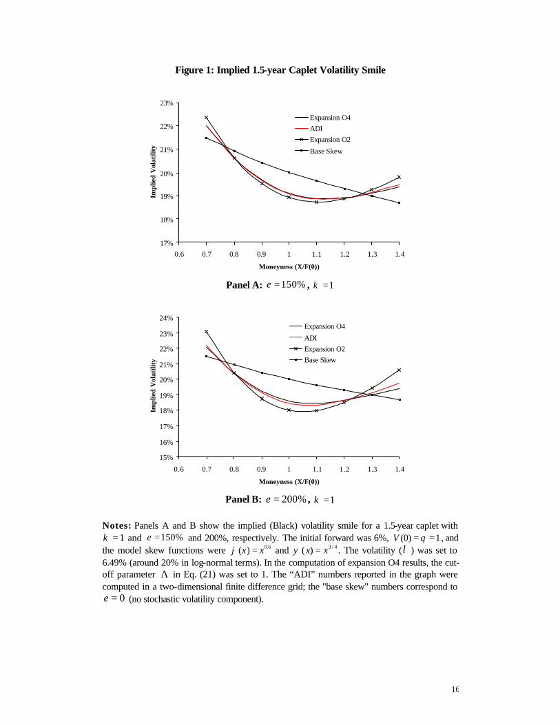
We note that for many typical parameters and option contracts, it often suffices to only include terms in (4) to order 2( )O ε (that is, set 0 1 2 0β β β= = = ), but the higher-order terms often become important when, say, the mean reversion speed ( )κ is low and the volatility-of-variance ( )ε is high. Figure 1 demonstrates typical performance of the

2( )O ε and 4( )O ε expansions (“O4” and “O2” in the figure). Many further tests can be found in Andersen and Brotherton-Ratcliffe (2001). 4. Exact Transform Solution.

In cases where very high volatility of variance and/or very low mean reversions are required, the expansions in Section 3 might have to be continued to inconveniently high order. In such situations it is sometimes safer and easier to instead rely on exact transform-based pricing expressions. To develop such expressions, however, we must simplify our setup somewhat. In particular, we specialize to an affine setting with ( )x xψ = and

( ) (1 )x mx m Lϕ = + − , where 0L ≥ and 0 1m< ≤ . As we shall show, this setup is tractable, although the tractability comes with the cost of permitting interest rates can become negative with positive probability. We also notice that the choice of ( )x xψ = allows the process (2) to reach 0 with positive probability if, as will often be the case in applications, 22κθ ε< . As 0 is non-absorbing, this has few practical ramifications, however.

As demonstrated in Section 3, caplet and swaption formulas have the same form in our setup; for variety we will here develop the latter. Dropping subscripts (i.e. , ( )s eR t becomes ( )R t , and so forth), we write

( ) ( )(0) (0)(0) (0) ( ) ( ) ' (0)A A

s s

A AS A E R T K E T K f

m mξ+ += − = − ≡

where ' (1 )K mK m L= + − and

( )( ) ( ) ( ), (0) (0) (1 )

( )d t

V t t mdW t mR m Lt

ξλ ξ

ξ= = + − .

Using the results of Heston (1993) and Lewis (2000) we find the swaption price formula by numerically solving the inverse Fourier integral

12

( )ln (0) / '

2 14

'(0) (0) (0, )2

i KK ef H dω ξ

ξ ω ωπ ω

− ++∞

−∞= −

+∫ (5)

where 1i = − and ( ; ) ( ; ) ( )( , ) a t b t V tH t e ω ωω += with ,a b given as the solutions to the Riccati ODEs

, ( ; ) 0s

dab a T

dtκθ ω= − = ,

2 2 2 2 21 12 2( ) , ( ; ) 0s

dbm t b b b T

dtλ ω κ ε ω= + − = .

7

For constant λ these ODEs can be solved in closed form (see e.g. Lewis (2000) or Lipton (2001)), a result which can also be used iteratively for piecewise constant λ . In the general case, a simple numerical Runge-Kutta scheme can be applied at little additional computational expense. We point out that the transform solution can easily accommodate non-zero correlation ρ between V and R by modifying the term bκ in the second ODE to

( )12( )b iκ ω ελρ+ − , but we shall rarely need this as non-zero correlation will hamper the

construction of practical models for the joint dynamics of the full yield curve (see footnote 1).

We finally note that when computing the integral (5) numerically, performance can often be improved by using the case 0ε = as a “control variate” through the split

( )

12 2 21

4

( )ln (0)/ '( ) / 2

2 14

'(0) (0) (0, ) '2

i Kv

BSK ef H e d K g

ω ξωξ ω ω

π ω

− ++∞ − +

−∞= − − −

+∫

where

( )(0)( ) 1 ( )

'BSg x xK

ξ− += Φ + − Φ ;

( )2 2 212 0

ln (0)/ ', ( ) ( (0) )

sT uKx v v m u V e du

vκξ λ θ θ −

± = ± = + −∫ .

With this trick, the combined scheme of Runge-Kutta and numerical Fourier inversion is fast and accurate, although some attention to step sizes is, as always, needed for long-dated options with strikes far from the at-the-money point. Typically, accurate option prices can be obtained in around 0.03 seconds per option on a regular PC (about three times faster for the constant parameter case). 5. A low-dimensional Markov model with stochastic volatility. In Section 2, we specified our stochastic interest rate model as an extension of the multi-dimensional Libor market model. In many cases, it is useful to work with approximating low-dimensional Markov models that allow for option pricing in finite difference grids. We shall here describe such a model which can be made approximately consistent with the cap and swaption expressions derived earlier.

As a starting point, let ( , ) ln ( , ) /f t T P t T T=−∂ ∂

be the usual continuously compounded forward rate at time t for deposit over the interval [ , ]T T dT+ . As shown by Heath, Jarrow, and Morton (HJM) (1992) any arbitrage free model with a single Brownian motion driving the yield curve level can be written as

( , ) ( , ) ( , ) ( )T

tdf t T t T t s dsdt dW tσ σ = + ∫

where W is a scalar Brownian motion under the risk-neutral measure and ( , )

T tt Tσ

≥ is a

collection of general stochastic processes adapted to the Brownian motion. The model is fully specified by the initial forward curve and a given volatility structure ( , )

T tt Tσ

≥. The

8

general one-factor HJM model requires as full continuum of all forward rates as state variables, with tree or lattice approximations of the model generally non-recombining and largely impractical.

Numerically tractable versions of the HJM model were treated in a range of papers in the early 90s, see for example Babbs (1993), Cheyette (1992), Jamshidian (1991), and Ritchken and Sankarasubrahmaniam (1992). In particular, it was noticed that when the forward rate volatility is of the separable form ( , ) ( ) ( )t T g T h tσ = where g is a deterministic function and h is some adapted stochastic process, a finite state variable Markov representation of the yield curve is possible. Specifically, defining

( ) '( ) / ( )t g t g tν = − and ( ) ( , ) ( ) ( )t t t g t h tη σ= = we get the bond reconstitution formula

21

2( )( , ) ( ) ( , ) ( )(0, )( , ) , ( , )

(0, )

u

tT s dsG t T x t G t T y t

t

P TP t T e G t T e duP t

ν−− − ∫= = ∫ (6)

where, in the risk-neutral measure, ( )( ) ( ) ( ) ( ) ( ) ( ), (0) 0dx t t x t y t dt t dW t xν η= − + + = , (7a)

( )2( ) ( ) 2 ( ) ( ) , (0) 0dy t t t y t dt yη ν= − = . (7b)

As long as ( )( ) , ( ), ( )t t x t y tη η= , (6) and (7a-b) show that the resulting model is Markovian in only two state variables, x and y. The first state variable x can be interpreted as a yield curve factor, with the instantaneous short rate given by ( ) ( , ) (0, ) ( )r t f t t f t x t≡ = + . The second state variable y has the interpretation of a convexity correction term ensuring that the model is arbitrage-free. It is worth noting that the model only collapses to a single state variable model in the case when η

is deterministic. In this case the model corresponds to the general Gaussian model as presented in, for example, Jamshidian (1991).

In traditional implementations of the model above it is customary to let the volatility of the yield factor be a function of the short rate, for example ( ) ( ) .pt r tη ∝ In this specification, however, the volatility skew induced by the coefficient p will tend to flatten for longer underlying tenors. To avoid this we here follow Andreasen (2000) and let η be a function of a longer tenor forward swap rate, i.e. ( ) ( , ( ))t t Y tη η= where Y is some forward swap rate, the identity of which can change over time. Which swap rate is chosen at

9

any point in time will depend on the instrument that we wish to price. For example when pricing a standard Bermudan swaption2 with final maturity eT we let , 1( ) ( ), [ , [k e k kY t R t t T T−= ∈ , whereas when pricing a Bermudan callable cap we could set , 1 1( ) ( ), [ , [k k k kY t R t t T T+ −= ∈ .

In any case, through (6), we would obviously have ( )( ) , ( ), ( )t t x t y tη η= . As a general rule, we notice that calibration and specification of low-dimensional Markovian models typically needs to be instrument-specific, unlike the Libor market models which are “large” enough to make possible calibration to the swaption and cap markets as a whole.

To incorporate stochastic volatility to our Markov model, we add to (7a-b) the third state variable V as given by (1b). The actual specification of our model is then ( )( ) ( ) ( ) ( )t V t t Y tη λ ϕ= ,

where λ is a deterministic function. As before, we will assume that 0dZ dW⋅ = .

For calibration of the model above to the swaption market closed-form or simple approximations for swaption prices are convenient. We note that under our assumptions the forward swap rate , ( )s eR t evolves according to

,, ,

( )( ) ( ) ( )s e

s e s e

R tdR t t dW t

xη

∂=

∂

where ,s eW is a scalar Brownian motion, and

1

, 1,

, ,

( , ) ( , )( ) ( , ) ( , ) ( , ) ( , )

( )( ) ( )

e

i i is e e e s s i s

s es e s e

P t T G t TR t P t T G t T P t T G t T

R tx A t A t

δ −= +∂ −= +

∂

∑.

To price swaptions we approximate this derivative as being approximately deterministic 3, and arrive at ( )*

, , ,( ) ( ) ( ) ( ) ( )s e s e s edR t V t t R t dW tλ ϕ≈ , (8)

( )( )

,*

, ( ) ( ) 0

( )( )( ) ( )

(0)s e

s e x t y t

Y tR tt t

x R

ϕλ λ

ϕ= =

∂= ∂

.

2 One might question whether it is sufficient to use only a single driving Brownian motion for the yield curve when pricing Bermudan swaptions. Andersen and Andreasen (2001) conclude that the answer is generally yes, provided that calibration of the mean reversion parameter ν is done carefully. 3 To understand why this is reasonable, we notice that if ,s e

R were the continuously compounded yield on a zero -coupon bond, it would be exactly linear in x.

10

We find that the approximation above provides sufficient accuracy for most applications, even for long-dated options out to, say, 30 years. Importantly, (8) allows us to use the results in Sections 3 and 4 to efficiently price swaptions and caps. Due to the structure of the model, once the mean-reversion of rate ν has been set4, the model volatilities ( )tλ can be bootstrap-calibrated to match a strip of swaption prices. On a standard PC, bootstrap calibration to, say, the swaption strip 1 29,2 28, ,29 1× × ×… can be done in less than 5 seconds when using transform inversion and in a few tenths of second using expansions (for comparison, the calibration can be done in less than one tenth of a second when volatilities are deterministic). Figure 2 demonstrates the quality of the fit for the case of

( ) (1 )x mx m Lϕ = + − , 0.2m = . 6. Numerical Methods. Numerical implementation of the general Libor market model (1a-b) presented in Section must virtually always be done through Monte Carlo simulation. Due to the zero correlation between the forward rate processes and the stochastic volatility process, it is possible to split the Monte Carlo generation of interest rate paths into two pieces: 1) draw a path of the variance process V through time; 2) draw a path of forward rates assuming that

( ) ( )k t V tλ is deterministic. Schemes for step 2) are well-known (see e.g. Andersen and Andreasen (2000)), so we here focus on simulating (1b) on some discrete time-grid

0,1,.. i it = . A direct Euler or log-Euler discretization of (1b) is prone to instability unless either

the time step or the mean-reversion parameter κ are small. Noticing the exact result ( ) ( ) 1( )

1( ) | ( ) ( ) i it ti i iE V t V t V t e κθ θ +− −+ = + −

it is generally better to resort to a moment matching scheme where, for instance, we can approximate 1( ) | ( )i iV t V t+ as a log-normal variable:

( )( ) 211 2

( ) ( )( )1

ˆ ˆ( ) ( ) i i ii i t t zt ti iV t V t e eκθ θ + − Γ +Γ− −+ = + − %

,

( ) ( )

( )( )1

1

2 2 ( )2 1122

2( )

ˆ( ) 1( ) ln 1

ˆ( )

i i

i i

t ti

t ti

V t et

V t e

κ

κ

ε ψ κ

θ θ

+

+

− −−

− −

− Γ = + + −

,

where the iz% ’s are a sequence of i.i.d. standard Gaussian draws. Monte Carlo schemes for the one-factor Markovian model presented in Section 5 are similar to those of the full LM model. Importantly, however, the limited number of state variables (a total of three) allows us to write down a low-dimensional PDE for option prices

4 To prevent the model from being too non-stationary, it is often best to let the rate mean reversion be constant. For instance, we could best-fit ν to reproduce the auto-correlation of the swap rates as computed approximately in a globally fitted LM yield curve model; see Andreasen (2000) for details.

11

which can feasibly be solved on a computer. Specifically, any contingent claim ϒ satisfies, subject to boundary conditions, the equation

0x y VD D Dt

∂ + + + ϒ = ∂ ,

where

2

21 13 2 2( ) ,xD r x y

x xν η

∂ ∂= − + − + +

∂ ∂

213 ( 2 ) ,yD r y

yη ν

∂= − + −

∂

2

2 21 13 2 2( ) ( ) ,VD r V V

V Vκ θ ε ψ∂ ∂= − + − +

∂ ∂

with (0, )r f t x= + .

The three-dimensional PDE above can be handled numerically using a number of available solvers. One good method which takes advantage of the fact that the PDE contains no mixed derivatives is the so-called Alternating Directions Implicit (ADI) finite difference method; see for instance the 3-dimensional Douglas scheme described Mitchell and Griffiths (1980). This scheme is uniformly stable, has the same order of computational effort as a multinomial tree, yet allows for complete freedom in grid design and has second order accuracy in the time-domain (as opposed to trees that only have first order time accuracy). Non-zero cross terms, i.e. correlation between the rates and the volatility, can be incorporated without loss of accuracy or stability but at a cost of making the scheme computationally more expensive5. In our implementation of the ADI scheme for the PDE above we use a standard three-point discretisation for the x - and V-dimensions, but a five-point discretisation for the y -dimension. This enables us to use a moderate number of grid points in the y dimension, around 10 or so, without sacrificing much accuracy. On a standard PC a 30-year Bermudan swaption can be priced in about 10 seconds in the stochastic volatility model. Switching off the stochastic volatility reduces the calculation time to about 0.5 seconds for the same contract. 7. Some empirical observations.

Estimation of the process (1b) is most easily done from observations of movements of implied volatilities (or their squares, the implied variances) of caps and swaptions. In particular, we notice that estimation needs to be done under a pricing measure, not the “real” historical measure, which makes traditional time-series estimation of historical volatility largely useless for our purposes.

The process (1b) implies that volatility of implied variance should decay with increasing option maturity, eventually reaching an asymptotic level. The asymptotic level is a

5 In certain special cases it is possible to change variables locally to eliminate the cross-terms, resulting in only a fairly moderate increase in computation time. More generally, we would need to modify the numerical scheme to explicitly incorporate correlation terms. Typical schemes for this (e.g. predictor-corrector schemes) would increase computation time by a factor of around two.

12

function of the skew specification ϕ ; the speed with which the volatility of implied variance approaches the asymptote is a function of the mean reversion parameter κ . Figure 3 demonstrates that this behavior is empirically observable for various swap tenors in USD. It is, however, obvious from the figure that the decay towards the asymptote is faster for short-tenor rates than for long-tenor ones. To make our model consistent with this behavior we find that we generally need mean-reversions κ of around 0.3-0.4 for medium-to-long-tenor rates in USD6, whereas short-dated rates (say, with tenors less than a year) are better fit with mean reversions of 1 or higher. It is also obvious from the figure that the volatility of variance parameter ε is higher for short-tenor rates than for long-tenor rates; in the US we find that rates with tenors less than 1-year typically require 150%ε ≈ , whereas longer-tenor swap rates are best described with 100%ε ≈ or less. The tenor-dependence of parameters can likely be explained as a diversification effect, as the variance processes of different forwards are, of course, less than perfectly correlated (which is what we effectively assume in our model with a single stochastic volatility factor). Still, we find empirically that movements of implied volatilities of most swap forward rates are quite high (typically above 80%, at least when the rate tenors exceed 3-5 years) and as such consider our setup a reasonable representation of reality. It is in principle not difficult to extend our LM model framework to multi-factor variance processes, but, as discussed earlier, the difficulties of populating the parameters of the model makes this of somewhat limited practical appeal.

Turning now to the question of how well stochastic volatility models can reproduce the observed volatility skews and smiles, we generally find that the model does a good job in both cap and swaptions markets. In Figure 4 we show typical fits for EUR and USD swaptions data. We typically find that parameters estimated from the historical decay-properties of volatility of implied variance are close to those required to match observed volatility smiles. In other words, out-of-the-money swaptions are priced approximately at the cost of vega-hedging with at-the-money swaptions. 8. Pricing Simple Exotics.

When applying stochastic volatility models to simple instruments, one can often get inspiration from the structure of the one-factor Markov model in Section 5 to come up with reasonable approximations. This, for instance, is useful when pricing European options on amortizing swaps, or options and swaps where the floating rate is a long-dated swap rate (so-called CMS rate). To illustrate this, consider the time 0 value (0)M of a CMS coupon paying a time7 sT the swap rate , ( )s e sR T :

( ) , ,, ,

,

(0)/ (0, )(0) (0, ) ( ) (0, ) ( )

( )s eA s e ss

s s e s s s e ss e s

A P TM P T E R T P T E R T

A T

= =

(9)

where ( )sE ⋅ as before denotes expectation under the martingale measure with the maturity

sT zero-coupon bond as numeraire.

6 In EUR, we generally find that mean reversions are slightly lower than in USD. See Figure 4. 7 We here ignore the fact that actual payments are typically made in arrears, that is at time 1s

T+ . The

adjustment for this payment delay can be performed using the same technique as shown here.

13

To evaluate (9) we need to be able to say something about the distribution of 1, ( )s e sA T− under the swap annuity measure. The idea is now to come up with an inspired

approximation for the annuity , ( )s e sA T as function of the terminal swap rate , ( )s e sR T and compute the expectation in (9) using earlier results. Dropping the subscripts on A and R, we first note that

( ) ( ) ( )2

( ) ( ) 0( )

( ) ( ) var ( ) var ( ) |s s

A A A ss s s s x T y T

R TE y T y T x T R T

x

−

= =∂ ≡ ≈ ≈ ∂

.

where ( )var ( )A

sR T is the variance in the annuity measure which can be implied from the swaption model of the first section. The swap rate derivative in the expression above can be obtained from a chosen level of rate mean-reversion ν . We can now use the reconstruction formula (6) to write ( ) ( )( ) , ( ), ( ) , ( ), ( )s s s s s s sR T R T x T y T R T x T y T= ≈ ;

( ) ( )( ) , ( ), ( ) , ( ), ( )s s s s s s sA T A T x T y T A T x T y T= ≈ .

As the first of these functional relationships is one-to-one, we get an expression

( ) ( , ( ))s sA T l T R T≈ , for some explicitly computable function l. To improve the approximation, we actually use ( )( ) , ( )s s sA T c l T R T= ⋅ (10)

where the constant c is chosen so that the Radon-Nikodyn satisfies the natural condition

( )

(0)/ (0, )1

, ( )A s

s s

A P TE

c l T R T

= ⋅

Equation (10) can now be inserted in (9) which again can be integrated on the density of R to value the CMS coupon. The density of R can, as always, be obtained by differentiation of swaption prices: ( ), 2 2 1

, , ,Prob ( ) [ , / (0; ) / (0)s eAs e s s e s eR T K K dK dK S K K A −∈ + = ∂ ∂ ⋅

where , (0; )s eS K is the time 0 price of a European payer swaption struck at K. Expressions for these prices have been derived in Sections 3 and 4. In Figure 5, we examine the performance of the above expression for different levels of mean-reversion ν . Notice that the convexity adjustments increase with mean reversion, a consequence of increased volatility of the short end of the curve (and thereby of the annuity A which has relatively short duration). 9. Pricing Exotics and Callable Instruments.

14

The techniques discussed in Section 8 are only useful for simple, European instruments. For more complicated instruments, such as Bermudan swaptions and other callable or path-dependent structures, the numerical methods discussed in Section 7 must be applied. For strongly path-dependent options, Monte Carlo simulation of the full Libor market model is the method of choice whereas Bermudan swaptions are probably best handled in a the low-dimensional Markov model coupled with an ADI finite difference solver. We do point out, however, that methods to price Bermudan/American options inside a Monte Carlo simulation of the full Libor market model exist (see e.g. Andersen and Broadie 2001 for a review) and will likely become more prevalent in the future as available computing power continues to increase.

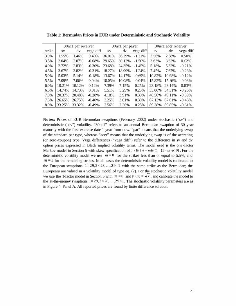
In Table 1 we use the ADI method to compare prices for 30 year Bermudan swaptions in the stochastic volatility model with those of the deterministic volatility model. Provided that the deterministic volatility model is calibrated to the European swaptions with strike equal to that of the underlying swap, the differences between Bermudan prices in the stochastic and deterministic volatility model are, perhaps suprisingly, not particularly significant.

References

Andersen, L. and M. Broadie (2001): “A practical primal-dual simulation algorithm for high-dimensional American options,” Working Paper, Gen Re Securities and Columbia University. Andersen, L. and J. Andreasen (2000): "Volatility Skews and Extension of the Libor Market Model," Applied Mathematical Finance, 7, 1-32. Andersen, L. and Andreasen, J. (2001). "Factor-Dependence of Bermudan Swaptions: Fact or Fiction?" Journal of Financial Economics, 62, 3-37. Andersen, L. and R. Brotherton-Ratcliffe (2001): “Extended Libor Market Models with Stochastic Volatility,” Working paper, Gen Re Securities. www.ssrn.com. Andreasen, J. (2000): “Turbo-charging the Cheyette Model,” Working paper, Gen Re Securities. Babbs, S. (1993):”’Generalised Vasicek’ Models of the Term Structure.” Applied Stochastic Models and Data Analysis, Vol 1, 49-62. Cheyette, O. (1992): “Markov Representation of the Heath-Jarrow-Morton Model.” Working paper, BARRA. Glasserman, P. and S. Kou (1999). “The term structure of simple forward rates with jump risk,” Working Paper, Columbia University

15

Heath, D., Jarrow, R. and A. Morton (1992): “Bond Pricing and the Term Structure of Interest Rates: A New Methodology for Contingent Claims Valuation.” Econometrica 60, 77-106. Heston, S. (1993): “A Closed-Form Solution for Options with Stochastic Volatility with Applications to Bond and Currency Options.” Review of Financial Studies 6, 327-344. Jamshidian, F. (1991): “Bond and Option Evaluation in the Gaussian Interest Rate Model.” Research in Finance 9, 131-710. Lewis, A. (2000): Option Valuation under Stochastic Volatility. Finance Press. Mitchell, A. and D. Griffiths (1980): The Finite Difference Method in Partial Differential Equations. John Wiley, New York. Rebonato, R. (2001), “The stochastic volatility LIBOR market model,” RISK, October, 105-110. Ritchken, P. and Sankarasubramaniam (1993): “On Finite State Markovian Representations of the Term Structure.” Working paper, Department of Finance, University of Southern California.

16

Figure 1: Implied 1.5-year Caplet Volatility Smile

17%

18%

19%

20%

21%

22%

23%

0.6 0.7 0.8 0.9 1 1.1 1.2 1.3 1.4

Moneyness (X/F(0))

Impl

ied

Vol

atili

ty

Expansion O4ADIExpansion O2

Base Skew

Panel A: 150%ε = , 1κ =

15%

16%

17%

18%

19%

20%

21%

22%

23%

24%

0.6 0.7 0.8 0.9 1 1.1 1.2 1.3 1.4

Moneyness (X/F(0))

Impl

ied

Vol

atili

ty

Expansion O4

ADIExpansion O2Base Skew

Panel B: 200%ε = , 1κ =

Notes: Panels A and B show the implied (Black) volatility smile for a 1.5-year caplet with

1κ = and 150%ε = and 200%, respectively. The initial forward was 6%, (0) 1V θ= = , and the model skew functions were 0.6( )x xϕ = and 3 / 4( )x xψ = . The volatility (λ ) was set to 6.49% (around 20% in log-normal terms). In the computation of expansion O4 results, the cut-off parameter Λ in Eq. (21) was set to 1. The “ADI” numbers reported in the graph were computed in a two-dimensional finite difference grid; the "base skew" numbers correspond to

0ε = (no stochastic volatility component).

17

Figure 2: Swaption Volatility Smile. Yield Curve Model versus Approximation

Notes: Sample of implied Black swaption volatility smiles of yield curve model (“Model”) in Section 5, vs. the approximation eq. (8). The yield curve model is calibrated to ATM European swaption prices in EUR (February, 2002) for the strip 1 29,2 28, ,29 1× × ×… . The graph use the simple displaced diffusion skew function ( ( )) ( ) (1 ) (0)R t mR t m Rϕ = + − , 0.2m = , and

( )x xψ = . Other process parameters were 1, 0.1, (0) 1Vε κ θ= = = = . In the full yield curve model prices are found by finite-difference solution.

6%

8%

10%

12%

14%

16%

18%

20%

-3% -2% -1% 0% 1% 2% 3%

Moneyness (K-R(0))

Impl

ied

Vol

atili

tyModel, 5x25

Approx., 5x25

Model, 15x15

Approx. 15x15

18

Figure 3: Volatility of Implied Variance of Various Rates in US

0.25 0.5 1 2 3 5 101

23

57

100

0.2

0.4

0.6

0.8

1

1.2

Volatility of Implied

Variance

Option Expiry

Tenor

Notes: The graphs shows the volatility of implied variance (= the square of implied volatility) implied for US swaptions on 1-, 2-, 3-, 5-, 7-, and 10-year rates, as estimated from two years of weekly data from Bloomberg.

19

Figure 4: Volatility Smile of Stochastic Volatility Model vs. Market

Panel A: EUR data, February 2002

Panel B: USD data, February 2002 Notes: the graphs show swaption smile as implied by a stochastic volatility model (2) and as observed in the market. The graph use the simple displaced diffusion skew function

( ( )) ( ) (1 ) (0)R t mR t m Rϕ = + − and ( )x xψ = . Parameters of the stochastic volatility process in USD were 0.3, 1, 0.3m ε κ= = = ; in EUR the parameters were 0, 1, 0.1m ε κ= = = . In both currencies we set (0) 1V θ= = .

5%

10%

15%

20%

-3% -2% -1% 0% 1% 2% 3%

Moneyness (K-S(0))

Impl

ied

Vol

atili

ty

Market 5x10

Model 5x10

Market 20x10

Model 20x10

5%

10%

15%

20%

25%

-3% -2% -1% 0% 1% 2% 3%

Moneyness (K-S(0))

Impl

ied

Vol

atili

ty

Market 5x10

Model 5x10

Market 20x10

Model 20x10

20

Figure 5: CMS Adjustment as Function of Expiry in EUR

Notes: CMS forward rate adjustment as function of maturity and rate mean reversion ν . The rate tenor is 20 years and the market is EUR, February 2002. The “Model” numbers were computed in a finite difference grid; the “Approximation” numbers were computed as outlined in Section 8. Model parameters were as in Figure 4, Panel A.

0.0%

0.1%

0.2%

0.3%

0.4%

0.5%

0.6%

0.7%

0.8%

0.9%

0 5 10 15 20 25

Maturity (Years)

For

war

d R

ate

Adj

ustm

ent

Approximation Modelapprox, kappa=0 ycm, kappa=0

v = 8%

v = 4%

v = 0%

21

Table 1: Bermudan Prices in EUR under Deterministic and Stochastic Volatility

30nc1 par receiver 30nc1 par payer 30nc1 accr receiver

strike sv dv vega diff sv dv vega diff sv dv vega diff 3.0% 1.55% 1.46% 0.40% 36.01% 36.29% -1.31% 2.56% 2.38% 0.50% 3.5% 2.04% 2.07% -0.08% 29.65% 30.12% -1.50% 3.63% 3.62% 0.02% 4.0% 2.72% 2.83% -0.30% 23.68% 24.35% -1.45% 5.18% 5.32% -0.21% 4.5% 3.67% 3.82% -0.31% 18.27% 18.99% -1.24% 7.45% 7.67% -0.23% 5.0% 5.03% 5.14% -0.18% 13.67% 14.17% -0.69% 10.82% 10.98% -0.12% 5.5% 7.09% 7.06% 0.04% 10.05% 10.08% -0.04% 15.82% 15.86% -0.03% 6.0% 10.21% 10.12% 0.12% 7.39% 7.15% 0.25% 23.18% 23.14% 0.03% 6.5% 14.74% 14.73% 0.01% 5.51% 5.29% 0.23% 33.86% 34.31% -0.26% 7.0% 20.37% 20.48% -0.28% 4.18% 3.91% 0.30% 48.56% 49.11% -0.39% 7.5% 26.65% 26.75% -0.40% 3.25% 3.01% 0.30% 67.13% 67.61% -0.46% 8.0% 33.25% 33.32% -0.49% 2.56% 2.36% 0.28% 89.38% 89.85% -0.61%

Notes: Prices of EUR Bermudan swaptions (February 2002) under stochastic (“sv”) and deterministic (“dv”) volatility. “30nc1” refers to an annual Bermudan swaption of 30 year maturity with the first exercise date 1 year from now. “par” means that the underlying swap of the standard par type, whereas “accr” means that the underlying swap is of the accreting (or zero-coupon) type. Vega differences (“vega diff”) refer to the difference in sv and dv option prices expressed in Black implied volatility terms. The model used is the one-factor Markov model in Section 5 with skew specification of ( ( )) ( ) (1 ) (0)R t mR t m Rϕ = + − . For the deterministic volatility model we use 0m = for the strikes less than or equal to 5.5%, and

1m = for the remaining strikes. In all cases the deterministic volatility model is calibrated to the European swaptions 1 29,2 28, ,29 1× × ×… with the same strike as the Bermudan; the Europeans are valued in a volatility model of type eq. (2). For the stochastic volatility model we use the 1-factor model in Section 5 with 0m = and ( )x xψ = , and calibrate the model to the at-the-money swaptions 1 29,2 28, ,29 1× × ×… . The stochastic volatility parameters are as in Figure 4, Panel A. All reported prices are found by finite difference solution.