YET ANOTHER ALGORITHM FOR PITCH TRACKING - Binghamton University
91
i YET ANOTHER ALGORITHM FOR PITCH TRACKING (YAAPT) by Kavita Kasi B.Eng. June 1999, Andhra University, India A Thesis Submitted to the Faculty Of Old Dominion University in Partial Fulfillment of the Requirement for the Degree of MASTER OF SCIENCE ELECTRICAL ENGINEERING OLD DOMINION UNIVERSITY December 2002 Approved by: ______________________________ Stephen A. Zahorian (Director) ______________________________ Vijayan Asari (Member) ______________________________ Glenn Gerdin (Member)
Transcript of YET ANOTHER ALGORITHM FOR PITCH TRACKING - Binghamton University

i
YET ANOTHER ALGORITHM FOR PITCH TRACKING
(YAAPT) by
Kavita Kasi B.Eng. June 1999, Andhra University, India
A Thesis Submitted to the Faculty Of Old Dominion University in Partial
Fulfillment of the Requirement for the Degree of
MASTER OF SCIENCE
ELECTRICAL ENGINEERING
OLD DOMINION UNIVERSITY December 2002
Approved by:
______________________________
Stephen A. Zahorian (Director)
______________________________
Vijayan Asari (Member)
______________________________
Glenn Gerdin (Member)

ii
ABSTRACT
YET ANOTHER ALGORITHM FOR PITCH TRACKING (YAAPT)
Kavita Kasi Old Dominion University, 2002
Director: Dr. Stephen A. Zahorian
This thesis presents a pitch detection algorithm that is extremely robust for both high
quality and telephone speech. The kernel method for this algorithm is the Normalized
Cross Correlation (NCCF) reported by David Talkin [16]. Major innovations include:
processing of the original acoustic signal and a nonlinearly processed version of the
signal to partially restore very weak F0 components; intelligent peak picking to select
multiple F0 candidates and assign merit factors; and, incorporation of highly robust pitch
contours obtained from smoothed versions of low frequency portions of spectrograms.
Dynamic programming is used to find the “best” pitch track among all the candidates,
using both local and transition costs. The algorithm has been evaluated using the Keele
pitch extraction reference database as “ground truth” for both “high quality” and
“telephone” speech. For both types of speech, the error rates obtained are lower than the
lowest reported in the literature.

iii
© 2002 Kavita Kasi. All Rights Reserved.

iv
This thesis is dedicated to Sri Saibaba, my parents and my advisor, Dr.Stephen Zahorian.

v
ACKNOWLEDGMENTS I wish to express my sincere gratitude to my thesis advisor, Dr. Stephen A. Zahorian, for
his invaluable advice, guidance, motivation and patience throughout the research work.
Without his support, this thesis would not have been possible. I also thank the National
Science Foundation, which partially funded the research under grant BES-9977260.
I would like to thank Dr.Vijayan Asari and Dr.Glenn Gerdin for graciously agreeing to
be on my committee and for their valuable time and generous assistance.
I would like to thank all my friends in the Speech Communication Lab for establishing a
positive working environment.
Finally, I wish to thank my family for their love and support in completion of my thesis.

vi
TABLE OF CONTENTS Page
LIST OF TABLES ..……........…………………………………………….............................ix
LIST OF FIGURES ...………………………………………………………………......…….x LIST OF EQUATIONS ..………………………………………........................……............xii
CHAPTERS
I. INTRODUCTION .......... ................................................................................................ 1
1.1 General Introduction………………………………………....................................1 1.2 Speech Production and Various Properties of Speech Signal..................................2 1.3 How Does Pitch Relate to Speech Production and what is Pitch Tracking.……....7 1.4 The Difficulty of Pitch Tracking……………………………………......................8 1.5 Basic Overview of Pitch Tracking Approaches.....……………………………......9 1.5.1 Pre-processing.....................…………………………………………............9 1.5.2 F0 Candidate Estimation.………………………………………….....................11 1.5.3 Post Processing..............……………………………………………..................13 1.6 Objectives and Overview of the Thesis.……………………………………..............14
II. BACKGROUND .......................................................................................................... .16
2.1 General Information……………………………………………………………...16 2.2 Survey of Existing Pitch Tracking Algorithms..……………………………........16 2.2.1 Comparison Study..............………………………………………...............17
2.2.2 Average Magnitude Difference Function (AMDF) Approach …………..................……………………………………………..........................18 2.2.3 Maximum Posteriori Pitch Tracking.....………………………………........20 2.2.4 Pitch Tracking for Telephone Speech Using Frequency Domain Methods ………................…………………………………………………………...........23 2.2.5 Application of Pitch Tracking for Prosodic Modeling to Improve ASR for Telephone Speech.………………………………………………………….........26
2.3 Summary............................……………………………………………................27
III. THE ALGORITHM.................................................................................. ........................28
3.1 General Overview of Pitch Estimation Steps..……………………………….......29 3.1.1 Pre-processing..............…………………………………………...............30 3.1.2 F0 Candidate Estimation..........…………………………………...............37 3.1.3 Candidate Refinement Based on Spectral Information…………...............42 3.1.4 Candidate Modification Based on Plausibility and Continuity Constraints …………......................…………………………………………………………..45 3.1.5 Final Path Determination Using Dynamic Programming ………...….........49

vii
3.1.6 Determination of Pitch Period Markers for Voiced Regions of the Speech Signals...........…………………………………………………………….............50
3.2 Summary……………………………………………............................................57
IV. EXPERIMENTAL VERIFICATION.............................................................................. 59
4.1 Introduction...........................…………………………………………….............59 4.2 Brief Description of The Test Database....………………………………….........61 4.3 Error Measures.....…………………………………………..................................63
4.3.1 Error type I.......…………………………………………….........................65 4.3.2 Error type II.........…………….…………………………….........................66 4.3.3 Error type III.....................…………………………………………............68 4.3.4 Error type VI....………………………………………….............................69 4.3.5 Error type V.......…………………………………………...........................70 4.3.6 Error type VI.............…………………………………………....................71 4.4 Results and Discussion........………………………………………......................72 4.4.1 Comparison With Results from Literature Survey……………………….. 82 4.5 Summary........................……………………………………………....................84
V. CONCLUSIONS AND FUTURE IMPROVEMENTS.................................................... .85
5.1 Overview...........…………………………………………….................................85 5.2 Conclusions and Future Work…………………………………………………..85
REFERENCES ....................................................................................................................... 88
APPENDIX VARIABLE NAMES AND HELP FILE........................................................ 91
1. Variable Names……..............….……………………………………….......................91 2. Help File……................…………………………………………….............................92
CURRICULAM VITA ........................................................................................................... 95

viii
LIST OF TABLES Table Page
2.1 Error rates indicating relative comparision of Maximum Likelihod,Vwaves and MAP Pitch Trackers……. …...............…………………………………..............23
2.2 Error table for the performance comparision of DLFT and Xwaves..…………...26 4.1 Pitch Tracking error summary for several databases to minimize BIG errors ….77
4.2 Pitch Tracking error summary for several databases to minimize GROSS errors ……….….………………………………………………………………………..78
4.3 Pitch Tracking error summary for several databases to minimize overall BIG
errors………………………………………………………………………….….79 4.4 Summary of BIG errors and Gross voiced errors for Keele database with different
controls….......................……………………………………………....................80 4.5 Parameter values for experiments….……….………………………....................81
4.6 Table of summary of performance of available algorithms……….......…............84

ix
LIST OF FIGURES Figure Page
1.1 Illustrations of physiologic components of human speech production ...................3 1.2 Illustrations of an acoustic speech signal, the spectrogram view and the voiced spectrogram view and the voiced-unvoiced portions of speech.….........................5 1.3 Illustration of adult human vocal track elaborating the mechanism of human
speech....………………………………………………………………...................6 1.4 Illustration of effect of center clipping on a typical speech signals.......................10 3.1 Illustrations of effects of nonlinear processing of speech signals on the F0 of
spectrogram of the signals….………………………............................................31 3.2 Presence of five prominent peaks for a pulse train with fundamental of 100 Hz for
four duty cycles……………………………………………………………..........33 3.3 Spectra of a highpass filtered pulse train illustrating the nearly eliminated
fundamental at 100Hz....……………………………............................................34 3.4 Spectra of absolute valued highpass filtered pulse train, illustrating the restoration
of missing fundamental………………………………………………………......35 3.5 Illustration of effect autocorrelation and NCCF signals on a typical voiced frame
of speech……………………………………………………………………........39 3.6 Illustration of the overall pitch tracking algorithm…............................................50 3.7 Illustration of the identified locations of the pitch period markers in the LPC
residual signal………………………………………………………………........52 3.8 Depiction of the overall pitch tracking algorithm in the form of flowchart ........54 4.1 Illustration where the reference contour contains non-zero pitch values while the
estimated contour contains zero pitch values (voiced to unvoiced errors) ...........66 4.2 Illustration where the reference contour contains zero pitch values while the
estimated contour contains the zero pitch values (unvoiced to voiced errors)......67 4.3 Illustration of final pitch contour estimation by the algorithm to represent the lack
of gross errors estimations as pitch halving or pitch doubling for a typical case ……………………………………………………………………..……………..73

x
4.4 Illustration of cases of pitch halving for Keele reference (Cntrl_1) and the subsequent correction by setting a threshold to create a second reference (Cntrl_2) ………………………………………………………............................................76

xi
LIST OF EQUATIONS Table Page
1.1 Equation illustrating the process of Center clipping.................….........................10 1.2 Equation illustrating the process of Auto Correlation.....................................…..11 1.3 Equation illustrating for the process of CEPSTRUM ..........................................12 2.1 Equation for Average Magnitude Difference Function (AMDF) Approach.........19 2.2 Equation for computing the pitch periods using modified Normalized Cross-
Correlation function…………………………………...........................................21 3.1 Equation for Normalized Cross Correlation function (NCCF)..............................37 3.2 Equation for Normalized Low Frequency Energy Ratio (NFLER).......................43 3.3 Equation for estimating LOCAL COST for dynamic programming.…................47 3.4 Equation for estimating TRANSITION COST for dynamic programming for
successive voiced frames…………………………...............................................47 3.5 Equation for estimating the TRANSITION COST from unvoiced to voiced
transition for dynamic programming………………............................….............48 3.6 Equation for estimating the TRANSITION COST from voiced to unvoiced
transition for dynamic programming………………….........................................48 4.1 Equation for calculation of Error Type I………………………………...............65 4.2 Equation for calculation of Error Type II………………………………..............65 4.3 Equation for calculation of voicing correlation ………....................................…68 4.4 Equation for calculation of Overall Big Errors………………………………......69 4.5 Equation for calculation of MEAN of Errors....…………………………….......70 4.6 Equation for calculation of STANDARD DEVIATION of errors .......................70

1
CHAPTER I INTRODUCTION
1.1 General Introduction
Speech has been the principal mode of communication throughout human history.
Both the vocal organs and our hearing mechanisms are intensely complex and
sophisticated systems well-suited for hearing and receiving oral messages. As acoustical
and physiological measurement techniques have evolved over the years, there has been a
considerable increase in the understanding of the speech and the hearing systems.
For quite some time, a significant amount of research work has been focused on
Automatic Speech Recognition [1]. Providing computers with the ability to speak has
also been the objective for a substantial amount of research. A primary underlying task is
the extraction of features from speech signals, which can be used for both recognition and
speech synthesis applications. One such very important feature is “fundamental
frequency,” more commonly referred to as “pitch.” Note that in this thesis, the terms
pitch and its primary acoustical correlate fundamental frequency are used
interchangeably.
Fundamental frequency (or F0, as it shall be primarily referred to in this document)
corresponds to the rate at which the human vocal cords vibrate.
Over the past thirty years, a number of F0 tracking algorithms have been
developed and reported [2]. This raises the obvious question of why new work is still
being carried out in this field. The complexity of F0 estimation stems from the variability
and highly irregular nature of human speech, as will be discussed in detail later. As a
consequence, none of the many reported algorithms have proved to be entirely
satisfactory; hence, researchers continue to strive for improved F0 estimation algorithms.
The research is motivated by the many applications for which a really robust pitch-

2
tracking algorithm could be used. Among these applications is the modeling of
“prosodic” features in speech, that is, modeling of qualities such as stress, emotion and
intonation patterns. Such information would be very helpful in, for example,
automatically determining questions from declarative statements. Another big reason for
renewed interest in F0 tracking is the many telephone applications for which speech
processing can be very useful.
1.2 Speech Production and Various Properties of Speech Signals
The human vocal organs are depicted in figure 1.1 to give a basic understanding of
how speech is produced and what the mechanism of the voice source is. The operation
of this voice source, shown below, determines F0.
Figure 1.1: Illustrations of the physiologic components of human speech production
[5].
The lungs act as reservoir and an energy source. When a person speaks, air is
pushed out from the lungs through the larynx into the vocal tract. To produce speech

3
sounds, this airflow is interrupted by the vocal cords or by a constriction of the vocal
tract.
From the point of view of F0 considerations, the most important part of the human
vocal system is the larynx, which contains the vocal cords, also known as the vocal folds.
It is the activity of the vocal cords that determines whether speech is produced as
“voiced” or “unvoiced” sounds. For voiced speech (all vowel sounds and parts of many
consonants), the vocal cords modulate the airflow with rapid openings and closings. The
rate of vibration of the vocal cords, known as the F0, depends primarily on the mass and
the tension of the cords. For the case of unvoiced speech (many consonants such as “s,”
“sh,” “z,” etc.), the vocal cords are positioned to allow a non-periodic turbulent flow,
and there is no periodic component in the resultant speech.
In Figure 1.2, the first panel depicts the time-domain representation of the signal
(“beet,” spoken by a male speaker). As can be seen in the figure, the voiced regions of
speech are clearly cyclic while the unvoiced regions are much more noise-like. The
second panel depicts the time-frequency-intensity representation (called a “spectrogram”)
of the same signal. Note the highly intense regions where the speech is voiced and the
less intense regions showing the unvoiced or the background sections of the speech
signal. The third panel illustrates what the signal looks like in the voiced regions of
speech. Note the highly cyclic pattern of the signal. It is these highly cyclic regions of
speech that help determine the F0.

4
Voiced speech
unvoiced/silence
Highly periodic regions that depict strong voicing
Figure 1.2: The top panel illustrates the acoustic speech signal and the middle panel
illustrates the spectrogram of the speech signal, while the bottom panel illustrates the
voiced and the unvoiced portions of speech.

5
For voiced speech, typical F0 ranges are of the order of 50-250 Hz for male
speakers, 120-400 Hz for female speakers and around 150-450 Hz for child speakers,
these ranges differ for different speaker conditions [6]. However, there are wide
variations from one individual to another. Even during the normal speech of a single
speaker, there can be pitch variations spanning from one to four octaves. These wide
variations, and other factors, make it very difficult to detect pitch with 100% accuracy
with any set of parameters.
Figure 1.3: Illustration of adult human vocal track elaborating the mechanisms
involved in human speech production [5].
The vocal tract is depicted in the figure 1.3. The function of the vocal tract is to
transform the signals from the vocal cords and other sources into intelligible sounds of
speech. This is achieved by modifying the shape of the vocal tract so that it produces
acoustic resonances specific to the desired speech sound. Thus, the relatively flat
envelope spectrum of the voice source is modified in shape to encode speech
information. Unfortunately, sometimes these resonances of the vocal tract make pitch
tracking more difficult, especially if the resonances are very prominent.

6
1.3 How does Pitch Relate to Speech Production and what is Pitch
Tracking?
Broadly speaking, speech features are divided into segmental features, which are
primarily indicators of very short speech events such as individual phonemes, and supra-
segmental features, which span a longer interval, such as a whole sentence or multiple
sentences. The supra-segmental features, also called prosodic features, include “pitch,”
“intensity” and “voice quality.” These prosodic features help convey meaning, emphasis
and emotions.
“Pitch” is the perception of overall frequency in a speech sound. The primary
acoustic correlate of pitch is fundamental frequency, which is directly determined by the
vocal cord vibrations. However, as mentioned above, typically the terms pitch and
fundamental frequency are used interchangeably. “Intensity” corresponds mainly to the
amplitude of the speech signal. “Voice quality” is defined as the combination of several
parameters including clarity, audibility and intelligibility. Pitch tracking consists of
determining whether speech is voiced and unvoiced, at each time instant, and if voiced,
what the F0 is for each time interval. Usually the primary interest is the overall pitch
track over a long interval such a whole word or sentence.
1.4 The Difficulty of Pitch Tracking
There are a number of factors that make accurate pitch tracking a very difficult
problem [7]. The fundamental reason is that the speech signal is not really periodic, and
it is highly non-stationary. That is, even over short time intervals on the order of 50 ms
the speech signal is often changing in F0, in amplitude and in overall spectral
characteristics. Generally speaking, the more rapidly varying the speech signal is, the
more difficult F0 tracking becomes since virtually all algorithms assume that speech is
not changing over some short analysis interval. Typically this analysis interval must be

7
long enough to contain at least a few pitch periods in order to take advantage of some
type of averaging to determine the pitch. In essence, the pitch-tracking problem is an
example of the fundamental time/frequency resolution problem, extensively studied in
signal processing. The pitch tracking problem is further compounded by the voiced
versus unvoiced decisions which must be made, and by some important applications
(telephone speech) for which the fundamental is absent or very weak. Even in normal
speech, for some cases, the first harmonic may be much larger than the fundamental,
which causes problems in many pitch trackers.
1.5 Basic Overview of Pitch Tracking Approaches
Each of the usual three steps involved in most pitch estimation algorithms are
briefly discussed in this section.
1.5.1 Preprocessing
The first step of pre-processing is usually low-pass filtering (cutoff = 600-1000
Hz) to remove the higher harmonics of the speech signal. Some algorithms also use a
linear predictive inverse filter to remove vocal tract resonances.
Another signal processing technique often used for pre-processing is center
clipping.
Center clipping is performed by setting the low amplitude sections of the
waveform to zero, while still preserving the shape of the larger amplitude pulses. This
operation tends to reduce the harmonic structure but preserve periodicity.
The operation can be described as:

8
(1.1)
clip_levelx(n)where0
clip_levelx(n)wherel)(clip_levex(n)y(n)
clippercentertheofoutputy(n)udemax_amplittheof
percentagefixedaiswhichlevelclippingtheclip_levelsignaltheofamplitudemaximumudemax_amplit
signalspeechx(n)thatGiven
<=
>=
=
==
=
Figure 1.4: Illustration of how center clipping affects a typical signal. In the first
panel, an acoustic waveform of a vowel sound by a child speaker is depicted. The
second panel of the figure shows the same data after center clipping. The fundamental
frequency is more apparent in the second panel, as there are fewer non-fundamental
components.

9
1.5.2 F0 Candidate Estimation
Pitch tracking algorithms can be broadly classified into the following categories:
frequency domain based (e.g., power spectral density, cepstrum etc.); time domain based
pitch tracking (e.g., waveform pitch period labeling, time-autocorrelation etc.); or joint
time-frequency domain. We briefly discuss the autocorrelation and cepstrum method in
the remainder of this section. The auto-correlation approach is the most widely used
method for estimating the pitch of a periodic signal. Mathematically the auto-correlation
is given the formula:
∑−
=
+=KN
nknsnskAUTO
0)()()(
For 0≤ k ≤ K-1. (1.2)
Where,
s(n) = the signal.
s(n + k) = the time lagged version of the original signal.
Thus, auto-correlation basically consists of convolving a signal with a time-lagged
version of itself. To be useful, the auto-correlation must be computed over a wide range
of lag values. If the speech signal is periodic then the auto-correlation function will also
be periodic. For periodic signals, the autocorrelation function attains a maximum at
sample lags of 0, +-P, +-2P, etc., where P is the period of the signal.
A major limitation of the auto-correlation function is that it may contain many
other peaks other than those due to basic periodic components. For speech signals, the
numerous peaks present in the auto-correlation function are due to the damped
oscillations of the vocal tract response. It is difficult for any simple peak picking process

10
to discriminate those peaks due to periodicity from these “extraneous” peaks. The peak
picking is more robust if a relatively large time window is used, but has the disadvantage
that the rapid changes in pitch cannot be tracked properly.
As mentioned above, another method for pitch tracking technique is computation
of the Cepstrum, followed by peak picking over a suitable range. The Cepstrum is
defined as the inverse Fourier Transform of the short time log magnitude spectrum.
( )( )( )22log)( txFFc =τ
( )( )( )21 log)( txFFc −=τ (1.3)
Where,
X(t) = the input signal under consideration.
For voiced speech, the Cepstrum tends to have local maxima at times, kT,
corresponding to integer multiples of the glottal periods. The “log” in the Cepstrum
equation tends to flatten the harmonic peaks in the spectrum and thus leads to more
distinct peaks in the Cepstrum function, as compared to the peaks in the autocorrelation
function.
The interval of speech over which the spectrum and hence the Cepstrum has to be
computed introduces a number of flaws in the F0 candidate estimation. It requires a
relatively large time window over which the Cepstrum must be computed in order to
cover the F0 ranges of human speech. Thus, as for autocorrelation methods, in regions
where there are rapid changes in F0, the method does not perform well.
Some of the shortcomings in the auto-correlation method are overcome using the
cross-correlation function.

11
The Normalized Cross Correlation function is very similar to the auto-correlation
function, but is better able to follow the rapid changes in pitch and amplitude. The major
disadvantage is an increase in the computational complexity.
1.5.3 Post-Processing
There are a number of gross and fine errors that result in erroneous tracking of the
pitch. The most common gross errors are pitch doubling and pitch halving. The pitch
doubling occurs whenever the first harmonic is mistaken for F0. Pitch halving occurs
when two pitch cycles are mistaken for a single cycle. This pitch halving occurs in
autocorrelation methods when the peak at a time lag corresponding to 2 F0 is large than
the peak at a lag corresponding to F0. The other main type of gross error is a mistake in
the voicing decision—either voiced speech is classified as unvoiced or unvoiced speech
is classified as voiced. Post processing is otherwise called as gross error reduction as
well.
One traditional post-processing step, intended to remove some of the gross errors
in F0 candidates, is median smoothing of the pitch contour obtained from a succession of
frame-based measurements.
Median smoothing does introduce some unwanted overall smoothing, although it
has been found to be more effective than a linear low-pass filter. Small deviation errors
are less of a problem.
1.6 Objective and an Overview of the Thesis
The basic objective of this thesis is to develop yet another pitch tracking
algorithm, with desirable properties as follows:

12
1. To obtain higher accuracy, for both studio quality and telephone speech, than for any
pitch tracker previously reported in the literature with a single set of parameters for all
purposes.
2. The pitch tracking should be developed as a series of software routines, which can
easily be integrated with other speech processing applications.
3. The tracking should be based on multiple sources of information, from both the time
and frequency domain.
Note that the portions of this thesis work have been presented as a conference paper to
the International Conference For Acoustic Speech and Signal Processing (ICASSP 2002)
[8].

13
CHAPTER II BACKGROUND
2.1 General Information
Various pitch detection algorithms have been developed in the past [9]. While
some have very high accuracy for regions that the algorithm identifies as voiced, the
overall error rate is still high since many voicing decision errors are usually made. The
performance degrades even more as the signal condition deteriorates, such as for the very
important case of telephone speech. Hence, there does not yet appear to be a single pitch
determination algorithm that operates reliably and accurately for all applications.
Nevertheless, new work can benefit by first examining the existing algorithms.
Therefore, this chapter is devoted to a brief overview of some of the existing methods for
pitch tracking.
2.2 Survey Of Existing Pitch Tracking Algorithms
In the remainder of this chapter, five papers in the area of F0 estimation are
summarized. The first study is itself a survey of three different F0 estimation methods,
and the study compares the pros and cons of each method. The second study discusses an
error correction technique used for overall improvement in F0 tracking performance. The
third study discusses a new F0 estimation algorithm using a time-pitch energy
distribution based on predictable energy to improve the normalized cross correlation
function and hence improve the accuracy of F0 estimation. This paper also presents a
number of modifications that can be applied to the core method, which can also be
applied to other methods. Once such modification is the use of a variable frame length.
The fourth study discusses a new F0 estimation algorithm for telephone speech. The fifth
study uses the F0 estimation algorithm based on the algorithm from paper four. This

14
study has been mentioned to emphasize the potential use of prosodic features for speech
recognition, in this case a tonal language.
2.2.1 Comparison Study
Eric Mousset, William A. Ainsworth and Jose A. R. Fonollosa in “A comparison
of several recent methods of fundamental frequency and voicing decision estimation”
[10] compare a number of existing methods for F0 tracking, including time domain,
frequency domain and joint time-frequency domain methods. The conclusion of the work
is that no one algorithm out performs all the others, with respect to either global or
individual criteria. The authors present a performance evaluation of a SIFT based
algorithm, a Frobenius norm based method and two bilinear time-frequency
representation based methods. Of these last two methods, one uses the Born Jordan
Kernel and the other uses the cone kernel method. All the methods are compared using
databases that had been recorded and labeled for the purpose of comparing pitch tracking
algorithms.
The author claims that among the above mentioned algorithms, the simplified
inverse filter-tracking (SIFT) algorithm is best suited for inter-speaker variability. Hence,
in this section we only summarize the F0 estimation steps for the SIFT algorithm.
The SIFT algorithm is considered a time domain algorithm. The signal is first low
pass filtered and pre-emphasized to improve the accuracy of the LPC (Linear Predictive
Coding) inverse filter. The LPC coefficients are then used to inverse filter the signal to
remove the effects of the vocal tract resonances. In order to increase the amplitude of
the signal prior to inverse filtering, the signal for the voiced frames is weighted by the
energy ratio between the original and the pre-emphasised signal. This signal is then
again low-pass filtered and clamped to remove any DC components. The autocorrelation
is then computed. To account for the discontinuity of the F0 space, the auto-correlation is
interpolated and the F0 candidates are determined by simple peak picking. The
autocorrelation is first used to determine whether each frame is voiced or unvoiced. For

15
each voiced frame, each autocorrelation peak is marked and then validated or rejected
based on the relevance of the time interval between consecutive markers. It is this cluster
of markers that constitute the pitch track.
2.2.2 Average Magnitude Difference Function (AMDF) Approach
A probabilistic error correction technique is used in conjunction with an averaged
magnitude difference function (AMDF), in the pitch detection method discussed in
Goangshiuan S. Ying, Leah H. Jamieson and Carl D. Michell [11].
The signal is first pre-processed to remove the effects of intensity variations and
background noise by low-pass filtering the signal and then center clipping it for each
frame. The average magnitude difference function (AMDF) is a time domain based pitch
estimation method. It is said to have advantages of relatively low computational cost and
easy implementation. The function is computed as the normalized sum of the absolute
difference between the signal and its time-lagged version using:
( ) ( ) ( )
..max,1
,11
framepergeneratedvaluesAMDFofnumberMMj
where
jixixN
jAMDFN
innn
=≤≤
+−= ∑=
(2.1)
The AMDF is used for the initial pass of peak picking. In this method, multiple
candidates per frame are found. This gives rise to local maxima for each frame as well as
global maxima for the whole utterance. The pitch track is then found by considering
several constraints such as the highest ratio of the local maximum to the global maximum
among others.

16
Since these techniques can give rise to gross errors and voicing decision errors, a
global error correction technique was formulated to work in conjunction with the main
routine. The claim has been that this method provides a means to correct errors in pitch
period estimation and actually provides for fast and accurate pitch detection. In the
process, first an estimate of the distribution of initial pitch estimates for the entire
utterance is obtained from a set of initial local estimates. This distribution is then
approximated as a normal distribution. The pitch estimates for each frame are then
weighed by the normal distribution values. The pitch estimate with the highest “weight”
(computed a the product of the original AMDF peak values and the normal distribution)
is then considered to be the new correct pitch estimate for that frame. Thus, the estimates
located around the mean of the distribution are more likely to be chosen as final
candidates rather than those far away from the mean of the distribution.
2.2.3 Maximum Posteriori Pitch Tracking
Maximum posteriori pitch tracking algorithm [12] by James Droppo and Alex
Acero creates a time-pitch energy distribution based on predictable energy to improve the
normalized cross correlation function used in prediction of F0 estimates for an utterance.
The first step in this method is to band-pass filter the signal to remove any low-frequency
noise and to diminish the energy of the unvoiced frames, thus strengthening the voicing
decisions made. The algorithm uses the assumption that for a periodic signal, x(n), a
sample of the signal can be predicted from a series samples in the past.
The prediction of the pitch periods for each frame is computed using the modified
normalized cross correlation function given by:

17
∑ ∑
∑
−
−=
−
−=
−
−=
+++
−++
=1
2
2
12
2
22
12
2
)(*)(
)(*)(
)(N
Nn
N
Nn
N
Nn
Pntxntx
Pntxntx
Ps (2.2)
After pitch candidates are computed for each frame, the energy distribution
function is formed using the concept of predicting the energy of the present frame using
the previous pitch periods. Whenever spectral discontinuities occur in the signal, the
forward and backward prediction energies are used to predict the energy of the present
frame. The sub-harmonics are suppressed using a weighting factor less than one. This
is done since if the signal is periodic with a period of “P” around the time “T,” then it is
likely that peaks of comparable magnitude can be found at sub-harmonics of “P.” Since
such peaks can result in erroneous tracking, the weighting just mentioned is used. The
final decision for the pitch estimate is based on two passes of dynamic programming. The
first pass is used to select the best candidate for each frame; the second pass combines a
voicing decision module to determine whether or not a frame is voiced or unvoiced and
then determines the final pitch track estimate.
This performance of the MAP algorithm has been tested and compared to the
performance of a commercially available pitch tracker (Xwaves) and maximum
likelihood pitch estimation (Maximum likelihood) algorithm, on a database of 200
sentences each from one female (Melanie) and one male (Mark) speaker. The “ground
truth” was derived as the pitch estimates of the electro-glottogram (EGG) signal. There
are two types of errors reported, voicing decision errors (Err_1) and the standard
deviation of relative pitch errors (Err_2). The table that follows summarizes the errors for
the three pitch estimators and shows the improvement in performance of the MAP
algorithm compared to the other pitch estimators. All the errors are percentages unless
otherwise mentioned.

18
Err_1 Err_2
Pitch tracker Mark Melanie
Pitch tracker Mark Melanie
Maximum
likelihood
0.46 1.08 Maximum
likelihood
13.2 20.8
Xwaves 0.34 0.74 Xwaves 8.0 10.7
MAP pitch 0.23 0.27 MAP pitch 7.2 9.6
Table 2.1: Error rates (percent) indicating relative comparison of Maximum likelihood,
Xwaves and MAP pitch trackers.
2.2.4 Robust Pitch Tracking for Telephone Speech using Frequency Domain
Methods
The focus of this paper [13] is pitch tracking for telephone speech, due to the many
applications where ASR is uniquely important over the telephone. Since the fundamental
frequency is often weak or missing for telephone speech, and the signal is distorted and
noisy and overall degraded in quality, pitch detection for telephone speech is a difficult
task [13,14]. It is important that pitch routines overcome the difficulties associated with
these signal degradations and perform well even in a telephone environment.
In this paper the algorithm (Discrete Logarithmic Fourier Transform, DLFT), a
frequency domain based F0 estimation method uses a logarithmically sampled spectral
representation of speech signals. If the signal has periodic peaks spaced at period P, then,
on the log scale, the harmonic peaks appear at log P, log P + log 2, log P + log 3 etc. One

19
can obtain the F0 estimate by summing the spectral energy spaced by log 2, log 3 etc.,
which is essentially the same as correlating the spectrum with a pulse template that
includes the number of harmonics considered. To estimate ∆ log f0 and provide
constraints for ∆ log f0 and logf0, which are used for guiding the final pitch track, two
sets of correlation functions are used. One is the “template frame” and the other is the
“cross frame.”
A template-frame correlation function is defined as the correlation of the weighted
DLFT spectrum of a Hamming windowed impulse train (the template) and the µ law
converted DLFT spectrum. This function is then normalized by the signal energy. The
correlation maximum will now correspond to the difference of logf0 between the signal
and the template. A cross-frame correlation function is defined as the normalized
correlation of the adjacent DLFT signal frames. The maximum of this correlation
function now gives a robust estimation of the logf0 difference between voiced frames.
The two constraints defined by the “template frame” and “cross frame” correlation
functions are used to define the search constraints for dynamic programming for
estimating the final pitch track.
The performance comparison of the DLFT algorithm with a commercially
available pitch tracker (Xwaves) has been reported. Each of the pitch trackers were tested
on a speech database (studio and telephone quality speech) comprised of five female and
five male speakers each reading a story of approximately 35 seconds long. The “ground
truth” was a manually checked pitch track derived as the pitch estimates of the
laryngograph signal. The study reports “gross” errors, and the standard deviation and the
mean of the absolute errors. The gross error is defined as the percentage (usually 10-
20%) by which the computed pitch track differs from the “ground truth.” The mean and
the standard deviation of the computed pitch track from the “ground truth” are calculated
for the absolute value of deviation of the computed estimate from the “ground truth”
estimate.

20
The table below shows the numerical comparison of both the DLFT and the
Xwaves trackers for both the studio and the telephone quality speech. All the errors
reported are percentages unless otherwise mentioned.
Xwaves:v
Xwaves:UV Overall
CONFIGURATION Ger Mean(Hz) Std.(Hz) v->uv
Ger
Xwaves 1.74 3.81 15.52 6.63 ------ 8.37
Studio DLFT 3.24 4.61 15.58 ---- 1.01 4.25
Xwaves 2.56 6.12 25.10 20.84 ---- 23.41 Telephone
DLFT 2.10 4.49 14.35 ---- 2.24 4.34
TABLE 2.2: Error table for the performance comparison of DLFT and Xwaves.
2.2.5 Application of Pitch Tracking for Prosodic Modeling to Improve ASR for
Telephone Speech
Chao Wang and Stephanie Seneff, in their paper “A study of tones and tempo in
continuous mandarin digit strings and their application in telephone quality speech
recognition” [15], discuss the use the F0 tracking algorithm described in the above
paragraph [13]. They make use of parameters based on orthonormal decomposition of
the F0 contour for tone recognition in Mandarin speech. The performance evaluation
clearly suggests the potential use of prosodic features for improved speech recognition.

21
F0 tracking is thus especially important for ASR in tonal languages as Mandarin speech,
for which pitch patterns are phonemically important.
2.3 Summary
This chapter presented a brief overview of the existing algorithms for F0
estimation. The final study was to emphasize the use of a robust pitch-tracking algorithm
for speech recognition purposes.
CHAPTER III THE ALGORITHM

22
This chapter presents the complete algorithm developed in this thesis for pitch
tracking of speech. This chapter is divided into a number of sub-sections. Each sub-
section described deals with a single signal-processing step. The sections have been
arranged according to the order in which the various steps are implemented in the code.
This order of processing is generally the same as that previously reported for pitch
tracking, such as for the algorithms mentioned in Chapter II.
The algorithms described in this Chapter have been implemented and tested using
MATLAB ver5.3. For the convenience of the reader, who may wish to compare
algorithm descriptions with the actual code, the code has been provided in Appendix A.
Key variable names contained in the code are placed in parentheses when these
variables are referred to in the main body of this chapter. Note that the code in the
appendix also contains numerous comments, and explanations about each variable, so
that the code can be more easily understood, and re-used as part of other speech signal
processing applications. At the end of this chapter, a brief overview of the code is given,
including a description of which portions of the code contain the various signal
processing steps mentioned in this chapter.
3.1 General Overview Of Pitch Estimation Steps
Our algorithm consists of six main steps, as listed below:
3.1.1.Pre-processing
3.1.2. F0 candidate estimation
3.1.3. Candidate refinement based on spectral information (both local and global)
3.1.4. Candidate modification based on plausibility and continuity constraints
3.1.5. Final path determination using dynamic programming
3.1.6. Determination of pitch period markers for voiced regions of the signal.

23
Note that most pitch algorithms in the literature only mention 3 main processing
steps, pre-processing, frame-based pitch estimation, and post-processing. Step 1 above
is pre-processing, step 2 is analogous to frame-based pitch estimation, steps 3,4, and 5 are
post processing, and step 6 is a final algorithm designed to estimate even finer pitch
details, after the overall pitch track has been determined. The signal processing used to
implement each of these steps is explained in detail in the following paragraphs.
3.1.1 Pre-processing
The first step of preprocessing is to create two versions of the signal, the original
and absolute value of the signal. The motivation for the nonlinear operation (absolute
value) is illustrated in figure 3.1 and in the explanation and example that follow figure
3.1.
In figure 3.1 for a certain sentence, the low-frequency portion of the spectrogram
of the studio quality version of the signal is shown in the top panel, the same portion of
the spectrogram is shown in the middle panel for the telephone version of the same
sentence, and the bottom panel is the spectrogram of the telephone version of the signal,
but after the absolute value processing. Computed pitch tracks are overlaid on each
spectrogram, using the processing methods described in more detail later in this chapter.
This figure clearly illustrates that the F0 track computed from the absolute value
telephone signal is quite similar to the F0 track of the studio version of the sentence,
whereas the F0 track computed directly from the telephone version of the sentence is
mainly in error, apparently due to the missing fundamental. Similar effects were noted for
many other sample telephone signals. Even for the case of some studio quality signals,
the absolute value processing appeared to make the fundamental more prominent. The
general strategy adopted in the remaining steps of processing was to completely process
both signals (i.e. the original and the absolute value), computing multiple F0 candidates
from each one, and then ultimately determining a “single” best track.

24
Weak fundamental or missing fundamental Strong fundamental
Figure 3.1: Illustration of the effects of nonlinear processing of the speech signal on
the F0 of the spectrograms of the signals, as explained in the text. In the top panel
(studio quality), the fundamental is clearly apparent, but appears to be missing in the
telephone version (middle panel). The fundamental reappears in the absolute value
of the telephone version (bottom panel).
To more thoroughly illustrate the benefits of using the absolute value nonlinear
operation to partially restore the “missing fundamental” a straightforward MATLAB
simulation was performed. In particular, a 100 Hz fundamental pulse train was created
using a sampling rate of 5000 samples per second. These values correspond to a period

25
of 50 samples. The spectra of various versions of this pulse train, as listed below, were
examined and plotted over a frequency range of 0 to 500 Hz.
The cases considered were:
1. Original pulse train.
2. High pass filtered pulse train (100 point FIR filter with cutoff at 200 Hz.).
3. Pulse train after high pass filtering, and absolute value.
Additionally, each of the conditions a, b, c listed were repeated using duty cycles
of 10% (5 point pulse), 30% (15 point pulse), 40% (20 point pulse), and 50% (25 point
pulse). Spectral plots are given in figure 3.2 (original signal), figure 3.3 (highpass
filtered signal), and figure 3.4 (highpass filtered and the absolute value signal). In all
cases a 512-point FFT was used to compute the spectra of a 512-point signal, using a
Hamming window. The plots clearly indicate that the highpass filter removes the
fundamental component at 100 Hz, but that the absolute value operation restores this
fundamental for all cases except the 50% duty cycle square wave.

26
Figure 3.2: The five prominent peaks in the range (0-500 Hz) for a pulse train with
fundamental of 100 Hz, for four duty cycles as noted. The spectra have peaks at all
harmonics, except for the 50% duty cycle case (square wave), which has only odd
indexed harmonics.

27
Figure 3.3: The spectra of the highpass filtered pulse trains, illustrating that the
fundamental frequency component at 100 Hz has been nearly eliminated.

28
Figure 3.4: Spectra of the absolute value of highpass filtered pulse trains, clearly
showing that the “missing” fundamental of 100 Hz has been restored for all cases,
except for the 50% duty cycle pulse train.
Thus this Matlab simulation with a variable duty cycle pulse train (simplified
model of a speech signal) clearly shows that the nonlinear absolute value operation can
be used to restore a missing fundamental component. The results with real speech
signals, especially when computed pitch tracks were overlaid on the low-frequency
portions of spectrograms, also clearly illustrated that the nonlinear processing was
beneficial for pitch tracking for the case of weak or missing fundamental frequency
components.

29
The next processing step is band-pass filtering of both the original and absolute
value signals, using FIR filters for each case. The filter cutoff frequencies and orders
were determined empirically by inspection of many signals in time and frequency, and
also by overall pitch tracking accuracy. In the final version of the tracking algorithm,
filter orders and pass band edge frequencies are parameters which can be user specified
in a setup file, and actual values to use depend on the error measure which is to be
minimized, as discussed in chapter IV. Typically, 150-point filters with passbands of
approximately 100Hz to 900 Hz are used for each signal. Each of these band pass
filtered signal is then decimated by a factor of 2, provided that the original sampling
frequency is 11 kHz or higher. If the sampling rate is less than 11 kHz then the signal is
not decimated. Each of the signals is then broken into overlapping frames (typically 35-
55 ms in duration, with a frame advance of 10 ms), thus forming the signals for frame
based processing. Each of the signals is then (optionally) center clipped on a frame basis,
using a center-clipping ratio of up to 0.25. That is, for each frame, the maximum
absolute value of the signal is determined, and all signal values with absolute values less
than the center clipping ratio times this maximum are set to zero. As described
previously in chapter I, center clipping reduces the harmonic structure of the speech
signals while still preserving the fundamental. At this point, the frame level signal is
ready for initial F0 candidate estimation.
3.1.2 F0 Candidate Estimation
The two preprocessed versions of the signal, as mentioned above, are now
processed frame by frame. The fundamental assumption is that the speech signal is
stationary over a frame interval, and thus the voicing properties are well defined and
constant for the duration of each frame considered. However, as mentioned in chapter I,
one of the difficulties of pitch tracking is that this assumption is not entirely valid.

30
The basic signal processing used for each frame is an autocorrelation-type
processing followed by peak picking. That is, the correlation signal will have a peak of
large magnitude at a lag corresponding to the pitch period. If the magnitude of the
largest peak is above some threshold (about 0.6) then the frame of speech is usually
considered as voiced.
A modification to the basic autocorrelation [16], and the one used in this work, is
the normalized cross correlation function (NCCF), [17], defined as follows:
Given a frame of speech sampled, s(n), 0 ≤ n ≤ N-1
Then:
ke0e
∑KN
0=n)k+n(s)n(s
=)k(NCCF (3.1)
Where , 0 ≤ k ≤ K-1 ∑KN+k=n
k=n)n(2s=ke
As reported in [17], NCCF is better suited for pitch detection than the “standard”
autocorrelation function, more commonly used in pitch tracking algorithms [2]. As
compared to the normal autocorrelation, the peaks in the NCCF are more prominent and
less affected by the rapid variations in the signal amplitude. The advantage of the
NCCF over the autocorrelation in terms of peak definition is illustrated in figure 3.5.

31
Figure 3.5: Illustration of the autocorrelation and NCCF signals for a typical
voiced frame of speech. Note the well-defined peaks in the NCCF signal in the
second panel as compared to the peaks defined in the AUTO_CORR signal in the
third panel.
Despite the relative robustness of the NCCF for pitch determination, it is still possible
that the largest peak in the NCCF will not be at the “correct” lag, or that the magnitude of
the largest peak is not a reliable indicator of whether the speech segment is voiced or
unvoiced. That is, in the basic method for pitch tracking, it is the magnitude of the
largest peak that determines whether or not a frame of speech is voiced. If the frame of
speech is classed as voiced, then the lag corresponding to the highest peak is considered

32
to be the pitch period. Unfortunately, this basic method is prone to problems resulting in
a number of errors. For example, due to the harmonic structure of speech, as explained
before, the largest peak may occur at half or double the “correct” lag value, or sometimes
may even occur at a slightly different correct value.
In our approach, we assume that for voiced speech there will not only be a peak at a
lag corresponding to the F0 period, but also there may be additional peaks of even higher
magnitude at different lags. Based on this assumption, instead of identifying only the
single largest peak per frame the algorithm searches for multiple peaks (F0 candidates)
per frame for each of the two signals using a multi-pass search algorithm, as described
below.
Intelligent peak picking
In the process of developing the algorithm described in this thesis, a multi-pass
algorithm was developed for searching for multiple candidates per frame. This peak
picking method, which we call “intelligent peak picking,” is described in detail below.
Despite the ability of the intelligent peak picking to generally identify the “correct”
peaks, some errors remain, most of which are eliminated by the spectrographic methods
described below. On final experimental testing of the pitch tracking algorithm, it was
determined that not all the steps in the intelligent peak picking result in more accuracy of
tracking, and therefore the final algorithm allows these additional steps to be optionally
used as controlled by parameters in a setup file.
In the first pass of the search algorithm, all local peaks in the NCCF signal (over
lag values in the range of the maximum to the minimum F0 specified) are found. A point
in the correlation is considered to be a peak, if it is larger than L points (typically L=2) on
either side of the peak. Those peaks that have a magnitude greater than a specified
threshold (Merit_thresh1, typically .4) are further processed. Thus these large local
peaks are considered to be the potential F0 indicators and saved for further consideration.
Additionally, for those cases where there is a very large peak (i.e., a peak whose

33
magnitude is greater than Merit_thresh3, or typically 0.96), then all other peaks in the
same frame are eliminated or ignored. Note that the searching is done from a lower lag
to a higher lag, so that higher F0 values are first found. Thus this refinement is used to
reduce the likelihood of pitch halving problems. Such problems generally arise for
strongly voiced, highly periodic speech signals, for which the NCCF (or in general any
correlation) function usually has strong peaks corresponding to both F0 (low lag) and
F0/2 (high lag).
In the second pass of the search algorithm, all the peaks remaining from the first
pass are tested to determine if there are any “close” larger peaks. “Close” is defined as a
range of lag values of 2 milliseconds on either side of the peak in question. This step is
used to eliminate peaks that are close to even larger peaks, while still allowing the same
size peaks to be considered for further processing if they are not close to other peaks.
In the third pass of the search algorithm, each peak is tested to determine if there is
also a peak at a lag value corresponding to twice the lag value. When such cases are
found, the amplitude (or “merit”) of the peaks at the shorter lag values are increased by a
factor (Merit_boost, typically 0.10) since the presence of the peaks at higher lag values
are additional evidence that the peaks at the lower lag values correspond to the correct
pitch period of the signal.
The peaks still retained, with their associated merit values, are the F0 candidates
considered for the final F0 track. In those cases where no peaks are found which satisfy
the constraints just mentioned, the frame is considered to be unvoiced. Despite the
relative robustness of the NCCF and the intelligent peak picking mentioned above,
considerable experimental testing indicated that some errors still occurred in a final F0
track obtained from this information alone. Errors were most likely to occur for telephone
speech or weakly voiced sections of studio quality speech. Therefore, additional
information and processing, as described in the next two sections, was used to improve
the overall robustness of the algorithm.

34
3.1.3 Candidate Refinement Based on Spectral Information
For all signals examined, the patterns in the spectrogram appeared to clearly show
voiced versus unvoiced regions of speech, and clearly showed the approximate F0
contour.
In this section we describe the empirically determined methods used to compute an
additional measure useful for making voiced/unvoiced decisions [18], and methods used
to determine a very smooth pitch contour with extremely few gross errors. This very
smooth spectrographically based pitch contour is then used to help select the “correct”
NCCF based candidates. Spectrograms were computed for both the original and
nonlinearly processed versions of the signal, as mentioned above.
The normalized low-frequency energy ratio (NLFER) is the additional measure
computed to help indicate voiced versus unvoiced regions. The sum of absolute values of
spectral samples (the average energy per frame) over the low frequency regions is taken,
and then normalized by dividing by the average low frequency energy per frame over the
utterance.
In equation form NLFER is given by:
indexframe=jandectrogram,spofregions
frequencylowofmagnitudelog=j)x(i,indexfrequency=iframes,of#total=N
where
∑i∑j
j)x(i,N1
∑i
j)x(i,=NFLER
(3.2)
In general, NLFER is high for voiced regions, and low for unvoiced regions, with
a threshold value (Threshold1) of approximately 0.50 representing a good boundary
point between the two regions. Note, however, that final voiced/unvoiced decisions did
not use such a hard threshold. The smooth but robust pitch track is obtained using the
following steps:

35
1.The low frequency portion of the spectrogram is smoothed using a mask
approximately 60 Hz wide in frequency and 3 frames in time.
2. Simple peak picking is used to determine the first peak in the search range
(F0_min: F0_max). If no peak is found, the frame is assumed to be unvoiced.
3. The track found from step 2 is median smoothed with a 3-point median filter.
4. An estimate of the average F0, and standard deviation of F0, is computed using
the middle third (voiced frames are sorted in order of frequency) of the voiced frames
from step 3.
5. All voiced frames in the estimate from step 3, and all those frames that differ
significantly from the average F0, are replaced by the average F0 value.
6. The track from step 5 is again “median smoothed” with a 5-point median filter.
7. Simple heuristics are used to combine the two spectral F0 tracks to determine an
overall smooth track. For example, if the average F0 of one track is significantly lower
than the average F0 from the other track, the track with the lower F0 is used.
This spectrogram-based F0 track is then used to determine the validity of the F0
candidates from the NCCF and peak picking. For voiced frames in the speech, the F0
candidates from the NCCF are tested for “closeness” to the corresponding spectral F0
point. For candidates less than 1.5 F0_min away from the spectral F0 value, the merit is
increased by a factor of 1.25, whereas peaks far away from the spectral F0 are reduced in
merit according to distance. Candidates which are farther away than 1.5 * F0_min from
the spectral F0 track are eliminated from further consideration.
3.1.4 Candidate Modification Based on Plausibility and Continuity Constraints
The end result of the processing steps, mentioned above are the F0 candidate
matrix, a merit matrix consisting of the amplitudes of the NCCF peaks for each of the F0

36
candidates, an NLFER curve (from the original signal), and the spectrographic F0 track,
as explained in the last section. These data are used to obtain local and transition cost
matrices, from which the lowest cost pitch track through all available candidates can be
found using dynamic programming. Several processing steps, as outlined below, are used
to compute the two cost matrices.
The main idea is to use the sources of information mentioned in the preceding
paragraph so that (1 – local cost) is a rough measure of the correctness of each candidate
based on the local (i.e., individual frame) information, and transition costs reflect the
notion that F0 should not change too rapidly within a voiced region. Thus, to a first
approximation, the merits mentioned above are the primary factors, which determine
local costs, and frequency differences between successive (in time) pitch candidates are
the main factors, which determine transition costs. The proper assignment of costs is
made considerably more difficult by the fact that the speech stream typically contains
voiced and unvoiced regions, and it is generally unknown apriori which part of the
speech is voiced and which is unvoiced. Thus, for example, the transition between an
F0 value of 150Hz to 0 Hz (unvoiced) should be assigned a low transition cost if the 0 Hz
candidate frame is really unvoiced, but should be assigned a high transition cost if the 0
Hz candidate frame is really voiced. Before costs are computed from the candidate and
merit matrices, the following steps are used to modify these matrices, with the goals of
improving the cost computations.
First, the frames are pre-classified according to the NFLER as either definitely
unvoiced (region 1, NLFER <= .5) or probably voiced (region 2, NFLER > .5). Thus, for
the definitely unvoiced region (region 1), all F0 candidates are set to 0, and the associated
merit is set to 0.99. For region 2, which could be either voiced or unvoiced, every frame
is assigned at least one viable pitch estimate, and a single unvoiced candidate, and merits
for both voiced and unvoiced candidates are assigned to roughly approximate
probabilities of “correctness” for each candidate. The majority of frames for region 2
already have at least one voiced candidate remaining from the NCCF/peak peaking
candidate modification steps mentioned above. The merits of these candidates, already
on a 0 to 1 scale with highest merit values more likely to be the correct candidates, are

37
left unchanged. Additionally, for each frame in region 2, the spectral F0 is also
included as a candidate, with a merit set at a midpoint (Merit_pivot, typically = 0. 55).
The merit of the unvoiced candidate is set equal to [1 – (merit of best voiced candidate)].
Thus, frames in region 2 that have strongly voiced candidates (i.e., candidates with merit
values close to 1.0), the merit for the unvoiced candidate will be close to 0.0. However,
for frames in region 2 that do not have strongly voiced candidates (i.e., highest merit
values for voiced candidates are not much larger than .5), the unvoiced candidate will
have a higher merit value.
Local costs
After all of the merits are assigned, as mentioned above, the local cost is computed
as:
merit.-1 local = (3.3)
, using a single matrix operation in MATLAB.
Transition costs
The transition costs are computed according to the following algorithm. Note that
“i” is the present frame index in these equations:
1. For each pair of successive voiced candidates (i.e., non zero F0 candidates)
2min)_0(
2))1(0)(0((
min_0
)1(0)(0*05.0)(cos
F
iFiF
F
iFiFittransition
−−+
−−∝ (3.4)
2. For each pair of successive candidates, only one of which is voiced (i.e., for
voiced to unvoiced transition options),

38
)_()(cos frameunvoicedNFLERittransition ∝ (3.5)
3. For each pair of successive candidates, both of which are unvoiced, (i.e., for the
unvoiced to the unvoiced decision making),
)1(*)(∝)(cos iNFLERiNFLERittransition (3.6)
The various proportionality constants mentioned above, plus one additional
constant used to adjust the overall ratio of local to dynamic costs, were empirically
determined based on an inspection of several hundred sample recordings, and
minimization of various error measures, as discussed in chapter 4. These factors are
included as parameters in the setup file for running the pitch tracker. Typical values are:
1. k1 = 17.0, as proportionality constant for successive voiced frames.
2. k2 = .9, as proportionality constant for unvoiced to voiced transitions.
3. k3 = 1.5, as proportionality constant for voiced to unvoiced transitions.
4. k4 = 0.1, as proportionality constant for successive unvoiced frames.
5. k5 = 1.0, as proportionality constant to weight transition costs relative to local
costs.
3.1.5 Final tracking using dynamic programming
The four panels in figure 3.6 illustrate the overall algorithm. The panels illustrate
the steps involving the use of the NFLER; the modifications of the possible F0 candidate
estimates based on plausibility and continuity constraints and finally depict the final pitch
tracking based on the F0 candidates.

39
Figure 3.6: Illustration of the overall pitch-tracking algorithm.
3.1.6 Determination of Pitch Period Markers for Voiced Regions of the Speech
Signals
One possible use of a robust pitch tracking routine is to determine and analyze the
fine details of the pitch track. One particular application is an examination of pitch jitter,
or small variations in the pitch period from cycle to cycle. Since most pitch trackers,
including the one described in this thesis, use considerable averaging (such as that
implicit in correlation calculations), the fine details of the pitch are eliminated. However,

40
these details can be recovered if the computed pitch track is used in conjunction with an
acoustic signal to locate the "start" points of each glottal (pitch) cycle. In this section, a
technique to locate these start points is summarized.
The basic approach is to first compute the linear predictive residual signal using a
12th order LP inverse filter. This LP residual, for which the beginning of each pitch
cycles is indicated with a large peak, is then used to locate the endpoints of each pitch
period via peak picking. The peak picking is done on a frame-by-frame basis, for each
frame indicated as voiced by the tracker. The first step is in peak picking is to locate the
largest overall peak near the center of the frame, using the same procedure as described
above in the first step of intelligent peak picking. From this center peak, locations of
additional peaks on either side of the center peak were found, with the constraint that the
peaks be located approximately one pitch period apart (using the pitch values found from
the tracking).
In the following figures, an original speech signal, the LP residual signal, and the
resultant pitch markers, after modulation by the energy of the speech signal are
illustrated. Although this pitch-marking algorithm still needs additional refinements
(since errors do occur), this brief description is included as a starting point for future
work.

41
Figure 3.7: The first panel shows the acoustic signal, the second shows the LPC
residual signal and the third panel shows the identified locations of the pitch period
markers in the LPC residual.
All the algorithms mentioned in this paper were developed as a set of MATLAB
functions, designed for easy integration with other software. Key routines include one
for computing multiple F0 candidates and merits for each frame, routines for spectral F0
42
tracking, and a routine for overall tracking. Another routine determines individual pitch
period markers, given the pitch track.
Figure 3.8 depicts in form of a flowchart the order of processing carried out with
respect to the MATLAB routines used in the algorithm. The rectangular boxes depict the
different MATLAB routines used in the development of the algorithm. The arrowheads
depict the direction of the data passage. The different outputs of the signal processing
blocks are depicted within parentheses. Each output has been named and its functionality
described alongside. Note that the ** notation depicts that passing of defined or estimated
estimates along with the signals mentioned.

43

44
Ptch_trk.m: This main routine is used for pitch tracking of a series of files. This
routine uses three “set up” files. The first setup file, ptch-trk.dat, is the main setup file,
which contains the names of two other set up files (which here we call list.dat and ptch-
trk.ini) and some other basic information concerning file formats. “List.dat” contains a
list of the speech files to be processed. “Ptch_trk.ini,” described more fully below,
contains parameter values, which specify the various thresholds and other constants used
in the tracking.
Ptch_trk.ini: This file specifies the user-defined parameters such as the frame
length (frame_length), the frame space (frame_space), minimum fundamental frequency
(F0_min), maximum fundamental frequency (F0_max) and the Fast Fourier transform
length used (fft_length). It also holds parameters such as the filter order (Filter_order)
used for filtering the original signal (Filter_order_o) and the absolute valued signal
(Filter_order_a), filter cut offs for filtering the original signal (F_hp_o, F_lp_o) and the
absolute valued signal (F_hp_a, F_lp_a), where the lower band edge is given by F_hp
and the upper band edge is given by F_lp; the various thresholds that affect the voicing
and voiceless decision-making; and finally the weighting proportionality constants used
for formulation of the transition matrix (k1, k2, k3, k4 and k5), as described in detail
above.
Ptch_tls.m: This routine makes a call to the routines used for signal processing. It
is in ptch_tls.m that the two versions of the signal are created, namely the original signal
(sig_org) and the absolute valued signal (sig_abs). Ptch_tls.m also makes calls to the
F0_track.m and the dynamic3.m routines, the functions of which are explained below.
F0_track.m: The inputs to this routine are the two versions of the signal and the
user-defined parameters. This routine then computes the pitch candidates for the speech
signal in processing. This routine segments the signal to the frame level and makes calls
to the frame level routines, and also to the spectrographic pitch tracking routines. The
main outputs of the routine are the pitch candidate matrix and the associated merit
matrix. Other outputs include the smooth spectrographic pitch track and the normalized
low frequency energy ratio.

45
spec_f0_org.m: This routine, called from the F0_track.m routine, with an input of
the entire original signal, computes the smoothed spectral track (F_peak_org). In
addition to F_peak_org, the routine computes and has as output the minimum pitch for
the utterance (Speaker_min_org), maximum pitch for the utterance (Speaker_max_org),
and the standard deviation of the pitch (determined from voiced intervals only)
(Speaker_std).
spec_f0_abs.m: This routine is the same as spec_f0_org.m, except that it operates
on the absolute value signal and has some small differences in the details of the code.
F0_frame.m: The inputs to this routine are a single frame of signal and some user
defined parameters. The routine makes calls to crs_corr.m and cmp_rate.m to compute
pitch candidates and associated merits for each frame.
Crs_corr.m: This routine computes the Normalized Cross Correlation sequence
for each frame as explained above. The signal is first center-clipped.
Cmp_rate.m: The inputs to this routine are the normalized cross-correlation
signal and some user defined parameters. The main function of this routine is the peak
picking of the NCCF signal. The outputs are the pitch candidates and associated merits
for a single frame.
Dynamic3.m: The primary inputs to this routine are the pitch candidate matrix,
merit matrix, spectrographic pitch track, and the normalized low frequency energy ratio.
The routine first compute the local and transition cost matrices, and then it determines the
lowest cost pitch track. The output is the final pitch track of the overall algorithm.
periods.m, ptch_mrk.m: used to determine the pitch period markers for the
speech signal. The inputs to the routine are the LP residual and the computed pitch
track. The output is an array of the same length as the original speech signal, which is
all zero, except for "markers” at identified beginnings of each pitch period.

46
3.2 Summary
This chapter details the derivation and the implementation of the pitch-tracking
algorithm. Example plots depict the functionality of the F0 estimation method employed
in this thesis. An attempt has been made to address the problems associated with the
harmonic structure of normal speech. Pitch tracking problems resulting from the missing
fundamental in some normal and telephone speech are discussed and the procedures used
to correct these problems are presented. The step-by-step explanation of the main
routines in the thesis work is intended to enable the interested reader to be able to make
use of these routines.
The following chapter presents the results of an experimental validation of the
pitch tracking routines for a variety of databases.

47
CHAPTER IV
EXPERIMENTAL VERIFICATION
4.1 Introduction
Research on pitch extraction has been conducted for more than 30 years. The result
of this research is a number of pitch detecting algorithms for a variety of applications.
Performance comparison of these algorithms is very difficult as each study tends to be
carried out on a unique data set. Performance comparison between algorithms increases
further as the number of methods and algorithms currently available increase. Literature
has shown that “there exists not one algorithm, that works perfectly for every voice,
application and environmental condition.” [2]. The problem is further aggravated because
the evaluations are typically restricted to limited sets of algorithms because of the
availability of limited data sets.
Thus attempts have been made by researchers to provide a “reference,” often
called the “ground truth,” for a widely available speech corpus so that a performance
comparison of different algorithms can be made. This reference then provides a common
tool to estimate the accuracy of the pitch tracking algorithms. Providing “ground truth”
(as we shall refer to it from now on) for a given speech database, is an elaborate process.
In the next two paragraphs to follow, the process involved in extracting the “ground
truth” for a given speech corpus is described.
For some speech databases, the laryngograph signal, which is more directly
associated with the rate of vocal cords expansion and closure, has been simultaneously
recorded with the acoustic signal. The laryngograph signal can thus be used to establish
the durations of each individual vocal fold cycle for a given speech signal. Thus, the
instantaneous fundamental frequency value can be reliably estimated from the

48
laryngograph signal. A stream of such pitch values from an utterance plotted against the
time at which they occur gives us a pitch contour.
In establishing, the ground truth, first the pitch track is computed using the
laryngograph database. Then these pitch estimates are evaluated manually and corrected
as needed. First the microphone signal is compared to the laryngograph signal (Lx). In
cases where there appears to be corruption of Lx (acoustic signal shows voicing and Lx
does not, or vice versa), the pitch estimates are changed accordingly. It is this manually
checked pitch track that forms the “ground truth.” The track obtained when the
algorithm is run over original speech corpus (with no manual corrections) forms the “test
data.” Different types of errors are estimated when the “test data” is compare to the
“ground truth,” as discussed in more detail below.
Both qualitative and quantitative measures can be used to evaluate pitch detection
algorithms. Many of the existing algorithms give fewer errors with short signals such as
words, consonants or small sentences spoken for duration of few milliseconds. Usually,
pitch tracking performance is found to degrade as the complexity of the signal increases.
To be more specific, many pitch trackers work well with short CVC syllables and
isolated words but when conversational speech is involved, the errors reported are higher.
Sometimes the errors reported are also found to increase or decrease for certain speaker
conditions, such as accent, tonal quality, microphone quality used for recording,
background noise, etc. The same can be said about the degradation of the performance of
the algorithm when telephone speech is involved. Telephone speech usually lacks the
fundamental, makeing it extremely difficult to correctly track the pitch.
Keeping this in mind, the pitch detection algorithm reported in this thesis has been
tested over a wide range of databases. These include CVCs, isolated words and sentences
spoken by a large variety of speakers (male, female and child speakers) over a range of
speaker and signal conditions. An attempt has been made to optimize the algorithm to
function reliably for a variety of conditions.

49
4.2 Brief Description of the Test Database
The overall robustness and accuracy of this algorithm was tested using four
databases. The databases used for testing are VOWEL-CVC, TIMIT-NITIMIT,
MOCHA, KEELE studio and KEELE telephone databases. In the next few paragraphs, a
brief description about each database is given.
VOWEL-CVC is a database collected by the Speech Communication Lab in the
Electrical and Computer Engineering Department at Old Dominion University. The
CVC(s) are the consonant-vowel-consonant such as bag (e.g., “b” is a consonant, “a” is a
vowel, “g” is a consonant) while the VOWEL(s) are the English vowel sounds as “a,”
“e,” “i,” “o,” “u”. The database employed for testing the algorithm consists of 46
consonant-vowel-consonants and 46 vowels spoken by different child, female and male
speakers chosen at random.
The TIMIT-NTIMIT databases employed for testing consist of 10 male and 10
female speakers each having spoken 10 sentences, giving a total of 200 test sentences.
The sentences average about 2 seconds in length. The TIMIT sentences are the studio
quality signals recorded under low background noise. The NTIMIT are the telephone
quality signals recorded when the speaker’s voice has been transmitted over noisy
telephone lines and hence undergo signal degradation. Note that the overall database
consists of 10 sentences spoken by each of 630 speakers, but only the subset of 20
speakers was used for this study. These 20 speakers were the first 20 (alphabetically
listed) speakers from 8 major dialect regions of the United States, broken down by sex. A
speaker's dialect region is the geographical area of the U.S. where they lived during their
childhood years [19,20].
The MOCHA database from the Center for Speech Technology Research at the
University of Edinburgh consists of studio quality signals and their respective
laryngograph signals, among the others. The pitch estimates from the laryngograph
signals form the “ground truth” database for testing the algorithm with the MOCHA

50
database. The MOCHA database consists of 460 sentences each by a male and a female
speaker. Speech signals in the database average 300 ms in length [21].
Keele University, UK provided the KEELE database, consisting of 10 sentences
spoken by 5 different male and 5 different female speakers. Speech signals average about
35 seconds in length. For algorithm evaluation purposes, the Keele pitch extraction
reference database was used. This reference database provides a reference pitch obtained
from a simultaneously recorded layngograph trace as the “ground truth.” This database
consists of studio quality speech signals sampled at 20KHz [22].
The Spoken Language Systems Group at the Laboratory of Computer Science at
the Massachusetts Institute of Technology, Cambridge, MA, provided the telephone
version of the KEELE studio database. This database consists of telephone quality speech
signals, formed by transmitting the studio quality speech signals through noisy telephone
and re-sampling at 8KHz.
4.3 Error Measures
In the following paragraphs we first define and then discuss the different error
measures involved in performance evaluation of the algorithm [23,24] presented in this
thesis.
In all, the performance of the algorithm is based on the following types of error
measures:
4.3.1. Voiced in reference track called as unvoiced in computed track (Error Type I).
4.3.2. Unvoiced in reference track called as voiced in computed track (Error Type II).
4.3.3. Overall big errors (Error Type III).
4.3.4. Mean of the errors between the reference and computed track (Error Type IV).

51
4.3.5. Standard deviation of the errors between reference and computed track (Error Type V).
4.3.6 Gross errors (Error Type VI).
In equations that follow, the following notations are used.
Fx = The reference F0 track.
Fe = The estimated or computed F0 track.
length( ) = The length of the reference F0 track. Fx
length( ) = The length of the estimated F0 track. Fe
For the following notations, all the non-zero pitch values in the reference track are
denoted by logic 1 and the zero values in the F0 tracks are denoted by logic 0.
length( ≠ ) = The length of non-zero reference F0 track. Fx 0
length( ≠ ) = The length of the non-zero estimated track. Fe 0
length( 0≡ ) = The length of zero reference F0 track. Fx
length( ≡ ) = The length of zero estimated F0 track. Fe 0
An explanation of each of the error types mentioned above is provided in sections
4.3.1 onwards:
4.3.1 Error Type I
When Fx is non-zero while is zero, then a voiced regions is incorrectly
classified as unvoiced by the pitch tracking algorithm gives rise to the voiced-unvoiced
error. The percent of this type error is determined by summing over all frames such that
such that Fe ≡ and Fx
Fe
0 0≠ , and dividing by the number of frames for which Fx
, as given below. Then the voiced to unvoiced error is given by: 0≠

52
Voiced_unvoiced_err = ( )
( )0 ≠Fx length0 ≡ Fe and 0 ≠Fx length
(4.1)
Non-zero pitch values
in the reference signal.
Corresponding zero
pitch values in the
estimated signal
Figure 4.1: Illustration where the reference contour contains non-zero pitch values
while the estimated contour contains zero pitch values (voiced to unvoiced errors).
4.3.2 Error Type II
When Fx is zero while is non-zero, an unvoiced region is incorrectly classified
as voiced by the pitch tracking algorithm gives rise to the voiced-unvoiced error. The
percent of this type error is determined by summing over all frames such that Fe ≠
Fe
0

53
and Fx ≡ , and dividing by the number of frames for which Fx , as given
below.
0 0≡
Then the voiced to unvoiced error is given by:
Voiced_unvoiced_err = ( )( )0 Fx
0 Fe and 0 Fx ≡
≠≡length
length (4.2)
Zero pitch values in the range specified by the arrows in the
reference contour
Figure 4.2: Illustration where the reference contour contains zero pitch values
while the estimated contour contains non-zero pitch values (unvoiced to voiced
errors).
Non-zero pitch values in the range specified by the arrows in the
estimated contour

54
Thus the overall voicing decision errors which also forms a common grade for PDA
evaluation among researchers is given by the following equation:
Voicing errors
= Voiced_unvoiced_err + Unvoiced_voiced_err (4.3)
4.3.3 Error Type III
Calculation Of Big Error
When, the reference F0 track is non-zero and the estimated F0 track is also non-
zero then (i.e., and Fx 0≠ Fe 0≠ respectively), then the speech in that frame is
classified as “clearly voiced.”
In such conditions, the ratio Fx
FeFx − is first tested against a certain threshold. If
the conditions, as described below, are met then the algorithm is considered to have made
a “Big Error.”
The ratio is tested against thresholds of the order 0.2 and –0.2 according to the
following dictations:
If the ratio Fx
FeFx − 0.2, then the pitch tracking algorithm is considered to
have made a gross error in estimating the fundamental frequency of more than 20% of the
reference and the error categorized as pitch halving. These types of errors are
categorized as gross_low_err and are used as defined later.
≥
Fx
In an otherwise case i.e. if the ratio Fx
FeFx − ≤ 0.2, then the pitch tracking
algorithm is considered to have made a gross error in estimating the fundamental
frequency of less than 20% of the reference and the error categorized as pitch Fx

55
doubling. These types of errors are categorized as gross_high_err and are used as defined
later.
Otherwise the pitch-tracking algorithm is assumed to have estimated the
fundamental frequency with an acceptable accuracy.
The +/- 20% threshold of acceptability is chosen because all pitch-tracking
algorithms are expected to provide a pitch estimate within this range with due
consideration of time quantisation errors and the finite frequency resolution of the
analysis technique [10.].
All the frames for which the computed track does not satisfy the above mentioned
condition is noted and returned back as “Big error.”
Hence the overall big errors are calculated based on the following formula:
Overall Big Errors = Big Errors + Voicing Errors. (4.4)
4.3.4 Error Type IV
Calculation of Mean of the Errors
The mean of the errors is defined as the mean of the amount by which the
computed track differs from the reference track for all the clearly voiced frames. i.e. for
all cases where
Voiced_length = length ( Fx 0≠ and Fe 0≠ )
MEAN = ∑ (4.5) gthVoiced_len
-(Fe

56
Since the mean is computed using Fe – Fx, whenever the difference is a negative
value it indicates that the computed track has a lower pitch value as compared to the pitch
value of the reference track.
4.3.5 Error Type V
Calculation Of Standard Deviation Of The Errors
The standard deviation of the errors if defined as the standard deviation for all the
frames in which the computed pitch value differs from reference pitch value when both
the tracks are voiced.
Hence for every clearly voiced frame:
Voiced_length = length ( Fx 0≠ and Fe 0≠ )
STANDARD DEVIATION = ∑ gthVoiced_lenMEAN) - Fx)-((Fe 2
(4.6)
A large standard deviation means that there is a large difference between the pitch
values of the estimated pitch and reference pitch values.
These errors are then estimated for all the utterances in the database for each
speaker. The sum of the individual durations of such erroneous regions is expressed as a
percentage of the total duration of the unvoiced and voiced speech respectively for the
respective databases.

57
4.3.6 Error Type VI
Calculation Of Gross Errors
The overall gross errors are categorized for deeper probe into the algorithms
functioning as:
(a) Overall gross (a) error for voiced portion, with weighting.
(b) Overall gross (b) error in voiced reference, without weighting.
The overall gross (a) error for the voiced portion is defined as the sum of the
voiced_unvoiced_err, gross_low_err and gross_high_err (all as defined above), but
normalized by a weighting factor equal to the number of frames where the reference pitch
track is unvoiced. This error takes into account only the regions where the reference track
is voiced and therefore averages (over a database) are computed using weighting factors
proportional to the number of voiced frames in each reference sentence.
The gross error (b) is computed identically to gross error (a), except averages are
computed without weighting factors proportional to lengths of voiced portions. In
experiments, it was found that gross errors results were very similar with or without the
weighting. Results are reported for gross error (b), without weighting.
4.4 Results and Discussion
The algorithm described in this thesis is used to compute a pitch contour for each
utterance in each of the test databases mentioned above.
Considerable initial testing was done to check for the presence of gross errors such
as pitch halving and pitch doubling for a variety of speakers and speaker conditions. This
testing was done primarily with the shorter signals in the VOWEL-CVC database as
these short signals allowed more accurate visual inspection. Plots of each of the
following were first examined for each test utterance:

58
1. Time-domain signal
2. Spectrogram
3. The final pitch contour
When these plots were manually inspected for each frame of the signal, as
expected, the algorithm provided no gross errors as pitch halving or pitch doubling for all
the cases tested. It was found that the algorithm tracked pitch even in some weakly
voiced regions. The algorithm resulted in no gross errors for varied signal and speaker
conditions, at least for the 46 signals checked (Note that these type inspections did
indicate many errors in earlier versions of the algorithm, while it was under
development.). The signals used for the final testing with the CVC –VOWEL database
were those utterances for which pitch tracking had appeared to be most difficult with
earlier versions of the algorithm.

59
Figure 4.3: Illustration of the final pitch contour estimation by the algorithm to
represent the lack of gross error estimations as pitch halving and pitch doubling.
The time domain acoustic signal is plotted in the first panel, the second panel
shows the final pitch contour overlaid on the spectrogram of the signal.
The second round of testing was conducted with the TIMIT-NTIMIT databases. It
has been shown that the performance of any pitch tracker degrades for telephone quality
speech. Based on this notion, it was decided to test the algorithm over the telephone
signals and compare it with the performance of the algorithm for the studio quality
version of the same utterances. This was done since no “ground truth” was available for
this data, but it was felt that the pitch track for the studio quality versions of the sentences
would provide a reasonable ground truth, at least with respect to the telephone versions
of the sentences. The algorithm was first tested with the 200 TIMIT signals and the
pitch contour kept for the “ground truth.” Then the corresponding 200 telephonic
sentences (NTIMIT) were tested with the algorithm and the error results noted.
The third round of testing was done with the MOCHA database. This database, as
mentioned earlier, provides the microphone signal and laryngograph signals (plus other

60
signals not used in this work). As mentioned previously, the laryngograph signal closely
follows the vocal cord activity; hence, the laryngograph signals are processed by the
pitch-tracking algorithm to determine a resultant pitch contour, which can be considered
as the “ground truth” (LARYN). Note that this ground truth was not “manually altered”
as would have been the case for an available reference database. The pitch track extracted
from the microphone signal with the algorithm forms the test data. The test data was then
tested against the “ground truth” for the error calculations.
The fourth round of testing was done with the KEELE database for both the studio
(K_std) and the telephone database (K_tele). This database contains the ‘ground truth’
(Cntrl_1) and the microphone signal. With this ground truth it was found that the number
of frames in the ground truth and the test track did not exactly match, despite using the
same frame spacing as was reported for the ground truth. To match the number of frames
as determined by our algorithm to the number of frames in the ground truth, a small
number of unvoiced frames were inserted in the beginning and/or end of the ground truth
signal. Note that this number of frames was typically a very small number such as 2 or
3 frames, with tracks typically over 3000 frames in length. After this the errors were
computed and tabulated, for the various error types mentioned above.
The fifth round of testing was done with modified “ground truth” in the KEELE
database issue. Although the Keele database includes what should be a very reliable
control (which we call Cntrl_1), inspection of this track showed several instances of what
appeared to be pitch halving. This type of error is considered as a gross error, and to
avoid this type of error, a second “ground truth,” called Cntrl_2 was formed. Manual
frame level inspection showed that any values below 70Hz for the male speakers and
110Hz for the female speakers appeared to be pitch-halving errors. Hence a threshold
was set and all values below the 70Hz range for the male speakers and 110Hz range for
the female speakers were set to zero (unvoiced). This formed the Cntrl_2 as described
above. These thresholds were determined as averages based on all the speakers.

61
Figure 4.4: The upper panel (Cntrl_1) exhibits apparent pitch having for a number of
voiced frames. Using a threshold, to reduce these low pitch values to unvoiced,
(Cntrl_2, in the lower panel) eliminates most of these large jumps in pitch. This is a
typical example for a female speaker.
Tables of errors for all the databases mentioned above are presented here. The
errors are reported as percentages. The errors of most interest are the BIG ERRORS,
which gives a single overall figure of merit for the performance of the algorithm with
respect to large errors of any type. The error of next-most most interest is the GROSS
VOICED ERRORS, which indicates the performance of the algorithm in the voiced
sections of speech.
Each of these databases was tested with three different sets of parameters (listed in
Table 4.5). Each parameter setting was intended to minimize one of the error types
mentioned above. The tests are for different parameter settings are referred to as
Experiments I, II and III.
The results for Table 4.1 were obtained with parameter settings (see Table 4.5) that
were selected to minimize the big errors (Experiment I in the parameter table).

62
Type of
data
Type of
control
V_uv_err Uv_v_err Big
errors
Mean STD Gross_high Gross_low
K_std Cntrl_1 11.20 7.29 10.16 -0.23 11.12 1.54 0.21
K_std Cntrl_2 10.00 8.13 9.45 -1.13 7.54 0.61 0.22
K_tele Cntrl_1 22.73 5.73 15.31 -0.02 11.50 1.69 0.38
K_tele Cntrl_2 21.41 6.19 14.37 -0.63 8.95 1.18 0.39
MOCHA LARYN 4.92 6.18 6.17 0.42 7.43 0.71 0.33
NTIMIT TIMIT 18.37 4.22 12.06 -1.11 6.15 0.36 0.61
TABLE 4.1: Pitch tracking error summary for several databases mentioned above to
minimize BIG errors. The results are obtained by a simple (non-weighted) average of
all the utterances in each database. Parameters settings were adjusted to attempt to
minimize the BIG errors (Experiment I).
The results in Table 4.2 were obtained with parameter settings (see Table 4.5) that
were selected to minimize the gross voiced errors (Experiment II).
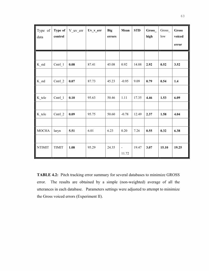
63
Type of
data
Type of
control
V_uv_err Uv_v_err Big
errors
Mean STD Gross_
high
Gross_
low
Gross
voiced
error
K_std Cntrl_1 0.08 87.41 45.08 0.92 14.88 2.92 0.52 3.52
K_std Cntrl_2 0.07 87.73 45.23 -0.95 9.09 0.79 0.54 1.4
K_tele Cntrl_1 0.10 95.63 50.46 1.11 17.35 4.46 1.53 6.09
K_tele Cntrl_2 0.09 95.75 50.60 -0.78 12.49 2.37 1.58 4.04
MOCHA laryn 5.51 6.01 6.23 0.20 7.26 0.55 0.32 6.38
NTIMIT TIMIT 1.08 95.29 24.35 -
11.72
19.47 3.07 15.10 19.25
TABLE 4.2: Pitch tracking error summary for several databases to minimize GROSS
error. The results are obtained by a simple (non-weighted) average of all the
utterances in each database. Parameters settings were adjusted to attempt to minimize
the Gross voiced errors (Experiment II).

64
Type of
data
Type of
control V_uv_err Uv_v_err Overall
Big
errors
Mean STD Gross
high
Gross
low
K_std Cntrl_1 12.56 7.96 11.25 0.09 11.19 1.69 0.15
K_std Cntrl_2 11.48 8.87 10.58 -0.93 7.09 0.68 0.16
K_tele Cntrl_1 27.47 6.25 18.60 2.47 14.73 3.39 0.23
K_tele Cntrl_2 26.22 6.69 17.63 1.82 12.26 2.91 0.23
MOCHA LARYN 4.06 4.50 4.65 0.09 6.18 0.42 0.24
NTIMIT TIMIT 14.36 4.69 10.02 0.37 5.39 0.53 0.13
TABLE 4.3: Pitch tracking error summary for several databases mentioned above to
minimize overall BIG errors. The results are obtained by a simple (non-weighted)
average of all the utterances in each database. Parameters settings were adjusted,
with the aid of visual inspection, to attempt to minimize the overall big errors
(Experiment III).
Summary of the different results obtained from different parameter settings are
depicted below for the Keele database with different controls.

65
Type of
data
Type of
control
Big errors
(Optimized)
Gross voiced errors
(Optimized)
K_std Cntrl_1 10.16 3.48
K_std Cntrl_2 9.45 1.35
K_tele Cntrl_1 15.31 6.19
K_tele Cntrl_2 14.37 4.09
Table 4.4: Summary of BIG errors and Gross voiced errors for the Keele database
with different controls. Note that different parameters settings were used to
minimize each type of error.
The different sets of parameters used for carrying out the different experiments
mentioned above are listed respectively in a separate table, Table 4.5. Note that the
software used a single file to control all these parameters.
Parameter Experiment I Experiment II Experiment III

66
Frame_length 50 35 35
F0_min 60 60 60
F0_max 450 450 500
Fft_length 1024 512 512
Filter_order_o 150 150 125
F_hp_o 25 25 150
F_lp_o 900 900 900
Filter_order_a 150 150 125
F_hp_a 50 15 100
F_lp_a 900 900 900
Merit_thresh1 0.4 0.3 0.3
Merit_thresh3 0.96 0.7 0.96
Merit_boost 0.1 0.1 0.0
Merit_thresh_final 0.1 0.40 0.40
Threshold1 0.1 0.5 0.5
Merit_pivot 0.45 0.55 0.55
K1 2.0 17.0 17.0
K2 5.0 1.0 0.9
K3 5.0 1.0 1.5
K4 5.0 0.1 0.1
K5 1.0 1.0 1.0
Merit delta 0.1 0.1 0.1
Clip ratio 0.00 0.0 0.25
Table 4.5: Parameter values used for Experiments.

67
4.4.1 Comparison with results from the literature survey
A thorough study of the available literature revealed that the MIT speech
laboratory, for the DLFT algorithm, reported the best errors analysis. The study was
reported using the KEELE database and hence provides a common ground for
performance comparison of this algorithm. The literatures also provided the error
measures for another pitch tracker XWAVES and therefore the XWAVES results are
included in this thesis to compare the performance of this thesis work with that
commercial tracker. A complete evaluation for the studio and the telephone speech
database, as given above, is compared with comparable results from the XWAVES and
MIT pitch trackers.
The following table compares the performance of the above-mentioned three
algorithms for the KEELE database (both studio and telephone). The error measures
reported are the Gross Voiced Errors (as defined above), the voiced (in reference) called
unvoiced (in computed track) (V_uv_err), and the mean and the standard deviation of the
pitch error for the voiced regions (when both reference and computed track are
considered voiced).
The YAAPT algorithm outperforms XWAVES for all error measures. The
YAAPT algorithm also has better performance in regard to the overall error as compared
to the DLFT algorithm by the MIT speech group in studio quality speech but the
performance of the DLFT is better than YAAPT for the telephone speech.

68
Type GER
(%)
V_uv_err
(%)
Mean
(Hz)
Std (Hz) Overall_err
(%)
Xwaves 1.74 6.63 3.81 15.52 8.37
DLFT
4.25
--
4.61 15.58 4.25
Studio
YAAPT
3.40 0.08 0.92 14.88 3.48
Xwaves 2.56 20.84 6.12 25.10 23.41
DLFT 4.34 --- 4.49 14.35 4.34
Telephone
YAAPT 5.99 0.10 1.11 17.35 6.19
TABLE 4.6: Summary of performance of the available algorithms.
4.5 Summary
In this chapter the various errors and the techniques used for the error analysis
were reported. A description of the possible values for the parameters that have been
used for obtaining the errors have also been depicted in a table.

69
In the next chapter a discussion of the possible future applications of this algorithm
and related routines is discussed in detail. The next chapter also provides a preview of the
likely enhancements that are likely to enhance the performance of this algorithm further.

70
CHAPTER V
CONCLUSIONS AND FUTURE IMPROVEMENTS
5.1 Introduction
In this thesis, Yet Another Algorithm for Pitch Tracking (YAAPT) was developed,
described and tested. The base frame level algorithm is based on the Normalized Cross
Correlation function as discussed in [2.]. YAAPT can be used to extract fundamental
frequency from speech signals with high accuracy. YAAPT can be used with other
speech processing algorithms and possibly be used to make improvements in end point
detection, or perhaps be used for pitch synchronous spectral envelope feature extraction
for vowel classification. This chapter discusses the achievements of the work and
outlines suggestions for future research.
5.2 Achievements and Future Work
The following conclusions can be made based on the results of the experiments
conducted. The research showed that the algorithm did not produce many big errors such
as pitch halving or pitch doubling. The various tests carried out on several databases
showed that the error rates obtained were very low. The algorithm proved to be robust
and accurate for a variety of speaker and signal conditions as well.
The use of the non-linear absolute value operation on the signal showed that in the
cases where the fundamental is weak or missing (such as for telephone signals), the
fundamental could be restored thus providing for better F0 tracking. The other non-linear
operation of center clipping also helped to improve the signal condition by reducing the
harmonics while still retaining the fundamental information. The use of the spectral
information for making a better voiced-unvoiced decision-making helped improve the
peak search algorithm as discussed in Chapter III. The spectrogram was also used to

71
provide a skeleton pitch contour to guide the peak search algorithm for picking the
correct F0 candidate.
Speech signals sometimes contain peaks of comparable magnitude at the correct
F0 period and also at double or half the correct lag value or simple at a different correct
lag value thus giving rise to small and large errors. These type problems motivated the
multi-pass peak searching approach.
The performance of the algorithm can be further improved by designing a robust
pitch- marking algorithm, i.e., the zero-cross detection algorithm based on the final F0
estimation. An attempt has been made in this research work to design an algorithm that
can detect pitch period markers from a time domain speech signal, with the goal of
finding an even more precise overall pitch track. The algorithm implemented is based
on intelligent peak picking of the LPC residual signal, using the information that the
approximate spacing between peaks should equal the already determined pitch period.
Although the method developed shows promise, further work is needed to improve
reliability. Ultimately this technique could be used to help estimate such important
quantities as pitch jitter.
The different parameter settings controls are available for the user. This enables
the user to adjust the algorithm for different applications tasks. Some applications require
only an estimate of the F0 information while others still require highly accurate F0
information. The different routines developed can be easily integrated with other speech
signal processing specific tasks as well.
In summary, a very accurate pitch-tracking algorithm has been developed. The
algorithm uses multiple estimates of the pitch, and associated merits, along with dynamic
programming to obtain a final result.

72
REFERENCES
[1] Zimmer, A., Dai, B. and Zahorian, S., Personal Computer Software Vowel
Training Aid for the Hearing Impaired, Proc. ICASSP 98, pp. 3625-3628,
Seattle, WA, May 1998.
[2] Wolfgang Hess, Pitch Determination Of Speech Signals, Springher-Verlag,
Berlin Heidelberg, New York, Tokyo, 1983.
[3] Rabiner, L. and Schafer, R., Digital Processing of Speech Signals, Prentice-
Hall, Englewood Cliffs, NJ, 1978.
[4] Oppenheim, A. V. and Johnson, D. H., Discrete Representation of Signals,
Proc. of the IEEE, vol.60, no. 6, June 1972.
[5] Lieberman, P. And Blumstein S., Speech Physiology, Speech Perception and
Acoustic Phonetics, Cambridge University Press, 1988.
[6] Baken, R., J. Clinical Measurement of Speech and Voice, Taylor and Francis
Limited, London, 1987.
[7] Jack, M. and Laver J., Aspects of Speech Technology, Edinburgh University
Press, Edinburgh, 1988.
[8] Kavita, Kasi, and Zahorain, S., Yet Another Algorithm For Pitch Tracking, Proc.
ICASSP 2002, Orlando, Fl, May 2002.
[9] Rabiner Lawrence R., Cheng, Michael, J. Rosenberg, Aaron E. And
McGonegal, Carol A., A comparative performance Study of several pitch
detection algorithms, in IEEE Transaction on Acoustics, Speech and Signal
Processing, Vol. ASSP-24, 399-417,No-5, Oct’76.
[10] Eric Mousset, William A. Ainsworth, Jose A.R. Fonollosa, A comparision of
several recent methods of fundamental frequency and voicing decision
estimation, ICSLP’96, pp. 1273-1276,Philadelphia.
[11] Goangshiuan S. Ying, Leah H. Jamieson, and Carl D. Mitchell, A Probabillistic
Approach To AMDF Pitch Detection, Proceedings of the 1996 International

73
Conference on Spoken Language Processing, Philadelphia, PA, Oct. 1996,
pp.1201-1204.
[12] Droppo, J. And Acero, A., Maximum a Posteriori Pitch Tracking, ICSLP’98,
Vol.3, PP 943, Sydney, Australia.
[13] Chao Wang and Stephanie Seneff, Robust Pitch Tracking For Prosodic
Modeling In Telephone Speech, ICASSP’00, Turkey.
[14] Moreno, PJ and Stern, RM, Source of degradation of speech recognition in the
telephone Network, ICASSP’94, May 1994, Adelaide, Australia.
[15] Chao Wang and Stephanie Seneff, A study of tones and tempo in continuous
mandarin digit strings and their application in telephone quality speech
recognition, Proceedings of the 5th International Conference on Spoken
Language Processing, Sydney - Australia, November, 1998.
[16] Cosi, P., Frigo, L., Mian, G. A., and Sinigallia, T., On The Use Of
Autocorrelation For Pitch Extraction: Some Statistical Considerations and Their
Application To The SIFT Algorithm, in Speech Communication, Vol.3, NO-4,
December 1984.
[17] Talkin, D., A Robust Algorithm For Pitch Tracking, in Speech Coding and
Synthesis, pp-495-518, 1995.
[18] Knorr, Siegfried G., Reliable Voiced/Unvoiced Decision, IEEE Transactions
On Acoustics, Speech, And Signal Processing, Vol.ASSP-27, June 1979.
[19] Charles Jankowski, Ashok Kalyanswamy, Sara Basson, and Judith Spitz,
NTIMIT: A Phonetically Balanced, Continuous Speech, Telephone Bandwidth
Speech Database, Proceedings of ICASSP-90, April 1990.
[20] Fisher, W. M., Doddingtion, G. And Goudie-Marshall, K.M., The DARPA
Speech Recognition Research Database: Specifications and Status, Proceedings
of the DARPA Speech Recognition Workshop, Report No. SAIC-86/1546.
[21] Manuel Rodrigues, Nick Roussopoulos, MOCHA: A Self-Extensible Database
Middleware System For Distributed Data Sources, Proceedings of the ACM

74
SIGMOD International Conference On Management Of Data, Dallas, Texas,
USA, May 2000.
[22] Plante F., Meyer G. And Ainsworth W. A., A pitch extraction reference
database, in EUROSPEECH’95, Madrid, pp. 837-840.
[23] Bagshaw, P., C., Miller S., M., Jack M., A., Enhanced Pitch Tracking and the
processing of the F0 contours for computer aided intonation teaching, Proc.
EUROSPEECH’93, Berlin, pp. 1003-1006.
[24] Bagshaw, P., C., Automatic Prosodic Analysis For Computer Aided
Pronunciation Teaching, PhD. Of Edinburgh University, 1994.

75
APPENDIX.
Variable Names and Help File
1. Variable Names
1. Threshold1 = the threshold value used to determine the voiced regions from the
unvoiced regions. Whenever the Normalized Low Frequency Energy Ration
falls below this threshold value, the region is termed as unvoiced; if it falls
above the value, it is termed as voiced region.
2. F0_min = the minimum F0 value being considered for estimation of F0 values.
It is set common for all speaker conditions.
3. F0_max = the maximum F0 value being considered for estimation of F0 values.
It is set common for all speaker conditions.
4. Merit_pivot = Whenever there occurs a region which probably maybe voiced, a
spectral F0 candidate is considered as the viable case and a merit value equal to
Merit_pivot associated with it.
2. Help File
2.1 Ptch_trk.hlp
creation date: January 2, 2002
revison date: April 6, 2002
Ptch_trk.m is the main routine used to compute the pitch track of a series of acoustic
wave files.
The input signals are files of the form *.wav, each of which should be an acoustic file in
either NIST or RIFF format.

76
The outputs are text pitch files, one for each waveform file. Note that the output files are
placed in the same directory as the waveform files are located in.
The setup files needed to run the program are:
ptch_trk.dat %Contains overall information
ptch_trk.ini %Some overall parameters for using the program
list.dat %List of files to process
Note that the names of the second two of these setup files can easily be changed, by
simply changing the names in the ptch_trk.dat file.
Sample files
// Sample setup file for pitch_trk
// Creation date: August 2, 2001
FILE_ID:PARAMETER_SPEC // FILE_ID must be on the first line
LST_FILE:bth_wav.dat // list of sentences
PAR_SPEC_FILE:ptch_trk.ini //setup file for pitch routines
FILE_TYPE:TYPEA1 //TYPEA1, TYPEB1, or HTK
2.2 Ptch_evl.hlp
creation date: April 6, 2002
revison date: April 6, 2002
Ptch_evl.m is the main routine used to evaluate the accuracy of the ptch_trk program.
The ptch_trk program must have first been run, and control pitch tracks must also be
located in same directories as pitch tracks.
The input signals are files of the form *.wav, each of which should be an acoustic file in
either NIST or RIFF format.

77
The outputs are text pitch files, one for each waveform file. Note that the output files are
placed in the same directory as the waveform files are located in.
The setup files needed to run the program are:
ptch_evl.dat % contains overal information
list.dat % list of files to process
Note that the names of the second of these setup files can easily be changed, by simply
changing the name in the ptch_evl.dat file.
Sample files
//Setup file for ptch_evl.m
//NOTE: Except the FILE_ID the rest of the files can be mentioned without any specific
order.
FILE_ID: PARAMETER_SPEC // FILE_ID must be on the first line
LST_FILE: std_ref.dat // list of pitch tracks
FILE_TYPE: TYPEA1 // TYPEA1, TYPEB1, or HTK
CURRICULUM VITA For

78
KAVITA KASI
NAME:
Kavita Kasi
DEGREES:
Bachelor of Engineering (Electronics and Communications Engineering),
Andhra University, Andhra Pradesh, India, July 1999.
PROFESSIONAL CHRONOLOGY:
Free Electron Laser Division
Thomas Jefferson National Accelerator Facility,
Newport News, Virginia.
Intern, January 2002-present
Department of Electrical and Computer Engineering
Old Dominion University, Norfolk, Virginia
Graduate Research Assistant, August 1999-May 2002
Student Support Services
Old Dominion University, Norfolk, Virginia
Graduate Teaching Assistant, August 1999-December 1999
SCHOLARLY ACTIVITIES COMPLETED:

79
Kavita Kasi, Zahorian, S. A., (2002), Yet Another Algorithm for Pitch Tracking,
International Conference on Acoustics, Speech, and Signal Processing, ICASSP 2002,
Orlando, Florida.

54
m
Data_org: original signal; **
THE FINAL PITCH TRACK
Spec_org_trk := pitch track from original signal. **
Spec_org_trk = pitch track from original signal. **
Pitch_array: F0 candidates for entire utterence. ; Merit_array: merit candidates for entire utterence. : NFLER:low frequency energy ratio; Est_track = estimated track from spectrogram processings from original and absolute valued. **
Frame_Rate = pitch
Frame_Rate = pitch candidates per frame. Crs_corr_sig: normalized cross correlated signal
**
Sig_part ; **
Sig_part = signal segmented into frames; Other defined/estimated
Data_abs: absolute valued signal ; **
Fs: sampling frequency. LenData: no. of data samples. Data_org : original signal. Data abs: absolute valued signal. **
Fs = sampling frequency. Data = the signal.
Dynamic.m
Cmp_rate.
Crs_corr.m
F0_frame.m
Spec_F0_abs.m Spec_F0_org.m
F0_track.m
Toolbox.m
Read_audio.m
Figure 3.8: Depiction of overall pitch tracking algorithm in form of a flowchart.