1/12

YEDITEPE UNIVERSITY ENGINEERING FACULTY

COMMUNICATION SYSTEMS LABORATORY

EE 354 – COMMUNICATION SYSTEMS

EXPERIMENT 3: SAMPLING & TIME DIVISION MULTIPLEX (TDM)

Objective:

Experimental verification of the sampling theorem; sampling and message

reconstruction. Time division multiplex (TDM) and its recovery.

Equipment:

Twin Pulse Generator Module

Audio Oscillator Module

Master Signals Module

Dual Analog Switch Module

Multiplier Module

Headphone Amplifier Module

Integrate & Dump Module

Oscilloscope

General Information:

Sampling is the first step of the transformation of an analog signal into a digital format.

Before it is possible to transmit analog information via a digital system the analog signal must

be first transformed into a digital format. Sampling can be made by two types of procedures. In

natural sampling, a slice of the waveform is taken and thus, the shape of the top of each sample

is the same as that of the message. In sampling with sample and hold, called also as flat top

sampling, a slide of the waveform is taken but the top of the slice does not preserve the shape

of the waveform. These two sampling types are compared in Figure 4.1.

Figure 4. 1 Natural Sampling (above) and Flat Top Sampling (below)

2/12

The arrangement to take samples of a sinewave is shown in Figure 4.2

Figure 4. 2 Sampling a Sine Wave

The natural sampling is shown in Figure 4.3 and the sampling by sample-and-hold is

shown in Figure 4.4.

Figure 4. 1 Natural Sampling

Figure 4. 4 Sampling by Sample-and Hold

3/12

Mathematical Review of Sampling

Using elementary trigonometry it is possible to derive an expression for the spectrum of

the sampled signal. The sampled signal is;

𝑠𝑎𝑚𝑝𝑙𝑒𝑑 𝑠𝑖𝑔𝑛𝑎𝑙 𝑦(𝑡) = 𝑚(𝑡). 𝑠(𝑡) (4.1)

where, 𝑚(𝑡) = 𝑉. 𝑐𝑜𝑠𝜇𝑡 is the message signal as a single cosine wave applied to the

input of a switch having the switching function 𝑠(𝑡) which is shown in Figure 4.5 and is

expressed analytically by the Fourier series expansion as;

𝑠(𝑡) = 𝑎0 + 𝑎1𝑐𝑜𝑠1𝜔𝑡 + 𝑎2𝑐𝑜𝑠2𝜔𝑡 + 𝑎3𝑐𝑜𝑠3𝜔𝑡 + ⋯ (4.2)

𝑠(𝑡) is a periodic function of period T = (2.π)/ω.sec. When 𝑠(𝑡) has the value “1” the

switch is closed, and when “0” the switch is open.

Figure 4. 2 The Switching Function

Expansion of 𝑠(𝑡), using equations (4.1) and (4.2), shows it to be a series of DSBSC

signals located on harmonics of the switching frequency ω, including the e zeroeth harmonic,

which is at DC, or baseband. The magnitude of each of the coefficients ai will determine the

amplitude of each DSBSC term. The frequency spectrum of this signal is illustrated in graphical

form in Figure 4.6.

Figure 4. 3 The Sampled Signal in the Frequency Domain

Inspection of Figure 4.6 reveals that, provided ω≥2µ, there will be no overlapping of

the DSBSC, and, specifically, the message can be separated from the remaining spectral

components by a low pass filter. This means that, if a signal is band limited, i.e., if its Fourier

transform is zero outside a finite band of frequencies, and if the samples are taken sufficiently

close together in relation to the highest frequency present in the signal, then the samples

uniquely specify the signal, and we can reconstruct it perfectly. This result is known as the

sampling theorem. This theorem also says that the slowest usable sampling rate is twice the

highest message frequency (ω≥2µ).

4/12

Reconstruction / Interpolation

From Fourier series analysis, and the consideration of the nature of the sampled signal,

it can be seen that the spectrum of the sampled signal will contain components at and around

harmonics of the switching signal and the message itself. Thus, a low pass filter can be used to

extract the message from the s samples. The reconstruction circuitry is illustrated in Figure

4.7.

Figure 4. 4 Reconstruction Circuit

If the reconstruction filter does not remove all of the unwanted components-specifically

the lower sideband of the nearest DSBSC, then these will be added to the message. Thus, the

unwanted DSBSC was derived from the original message. It will be a frequency inverted

version of the message, shifted from its original position in the spectrum. The distortion

introduced by these components, if present in the reconstructed message, is known as aliasing

distortion.

If message reconstructions by low pass filtering of natural samples results in no

distortion, then there must be e distortion when flat top pulses are involved. The pulse width

determines the amount of energy in each pulse, and so can determine the amplitude of the

reconstructed message. But, in n a linear and noise free system, the width of the samples plays

no part in determining the amount of distortion of a reconstructed message.

Time Division Multiplex (TDM)

In this experiment we will sample several messages, and their samples will be interlaced

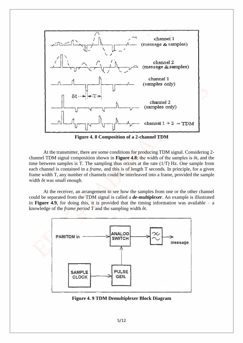
to form a composite, or Time Division Multiplexed – TDM signal. In Figure 4.8 the

composition of a 2-channel TDM signal is shown. If two messages were sampled, at the same

rate but at slightly different times, then the two trains of samples could be added without mutual

interaction.

5/12

Figure 4. 8 Composition of a 2-channel TDM

At the transmitter, there are some conditions for producing TDM signal. Considering 2-

channel TDM signal composition shown in Figure 4.8; the width of the samples is δt, and the

time between samples is T. The sampling thus occurs at the rate (1/T) Hz. One sample from

each channel is contained in a frame, and this is of length T seconds. In principle, for a given

frame width T, any number of channels could be interleaved into a frame, provided the sample

width δt was small enough.

At the receiver, an arrangement to see how the samples from one or the other channel

could be separated from the TDM signal is called a de-multiplexer. An example is illustrated

in Figure 4.9, for doing this, it is provided that the timing information was available – a

knowledge of the frame period T and the sampling width δt.

Figure 4. 9 TDM Demultiplexer Block Diagram

6/12

The switching function s(t) has a period T. It is aligned under the samples from the

desire channel. The switch is closed during the time the samples from the desired channel are

at its input. Consequently, at the switch output appear only the samples of the desired channel.

From these the message can be reconstructed.

To recover individual channels it is necessary to have a copy of the sampling clock. This

is generally derived from the TDM signal itself. The TDM signal contains no explicit

information to indicate the start of a frame. Channel identification is of course vital in a

commercial system, but we can dispense it for this experiment.

A PCM encoder is shown in Figure 4.10. Here, samples are coded into binary digital

words, and placed into frames of eight slots, each slot being of length equal to a bit clock period.

Each frame contained a coded version of a “flat top” sample of an analog signal (obtained with

a sample-and-hold operation), together with a frame synchronization bit.

Figure 4. 10 PCM Encoder Timing Diagram

If the contents of every alternate frame were removed from the serial data, then it would

appear that the sampling rate had been halved. Then, the allowable bandwidth of the signal to

be sampled would have been halved. The message could still be decoded if each alternate frame

could be identified. Thus, the empty spaces in the data stream could be filled with frames

derived by sampling another message. These would not interfere with frames of the first

message. Thus, two messages could be contained in the one data stream. This is a Time Division

Multiplexed Pulse Code Modulated (PCM TDM) signal.

7/12

Procedure:

1. Build the sampling system shown in Figure 4.2 for natural sampling. In order to

generate the switching function in the figure use the TWIN PULSE GENERATOR

module. Take the sampling frequency as 8.333 kHz. Observe the message signal and its

sampled version on the oscilloscope and draw them on a scope sheet.

2. Recover the message signal by using the LPF output of the HEADPONE AMPLIFIER

module which has the response of a 3 kHz LPF. Draw the recovered signal on a scope

sheet.

3. Change the frequency of the message signal within the full frequency range of the

module used for message signal generation. Explain the significant changes, if any, on

the reconstructed signal as the message frequency changes.

4. Observe the changes when the width of the switching pulses is changed. Comment on

the results.

5. To realize flat top sampling, use the INTEGRATE & DUMP module. Draw the

waveforms of the message signal and the sampled signals on a scope sheet.

6. Use the TUNABLE LPF module to recover the message signal. Turn the tune knob of

the TUNABLE LPF within its full range and explain the significant changes, if any, on

the reconstructed signal.

7. Use 2 kHz sinusoidal signals to observe a 2-channel TDM signal on the oscilloscope

and draw the waveform on a scope sheet. Take the sampling frequency as 8.333 kHz.

8. Change the time and the width of the samples of the input signals and draw again the

waveforms on a scope sheet.

9. Build the circuit of Figure 4.9. Observe the resulting waveform on the oscilloscope and

draw it on a scope sheet.

10. Pass the TDM signal through a LPF and observe the result on the oscilloscope. Draw

the scheme on a scope sheet.

8/12

YEDITEPE UNIVERSITY

DEPARTMENT of ELECTRICAL & ELECTRONICS ENGINEERING E X P E R I M E N T R E S U L T S H E E T

Course: EE 354 Communication Systems Experiment : 3 Semester: 2016 Spring

Group Information

Group No

Date Lab. Instructor’s Notes

Student Signature

Student No Student Name

1

2

3

4

SAMPLING & TIME DIVISION MULTIPLEX (TDM)

PROCEDURE 1. Build the natural sampling system in Figure 4.2 (see Experiment

Sheet). In order to generate the switching function in the Figure 4.2, use the TWIN PULSE

GENERATOR and DUAL ANALOG SWITCH modules. Take the sampling frequency as

8.333 kHz. You can use AUDIO OSCILLATOR module as a message signal with a variable

operation frequency.

Select an appropriate message frequency to obey Nyquist Criteria!

CHANNEL 1

(Message signal)

............. V/Div

............. s/Div

CHANNEL 2

(Sampled signal)

............. V/Div

............. s/Div

Message Signal at ……. Hz.

Sampling Frequency at 8.333 kHz.

9/12

Comment: What are the maximum operation frequencies of the message signal to

obey Nyquist Critea? Explain, briefly.

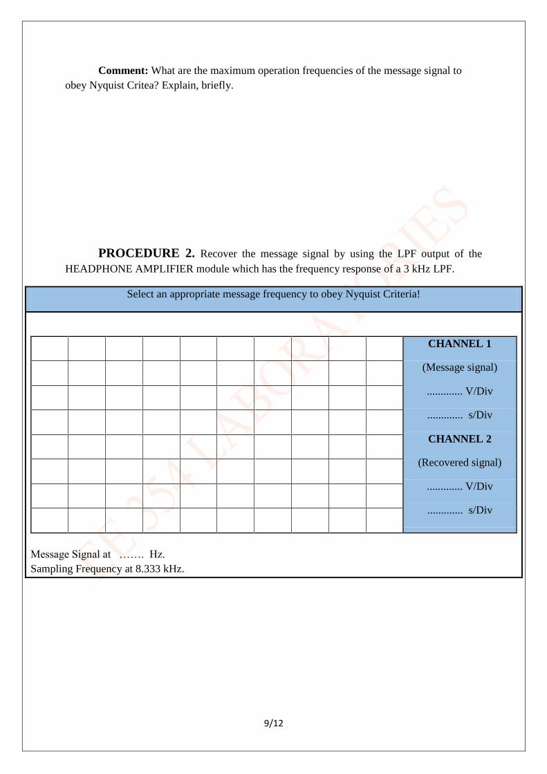
PROCEDURE 2. Recover the message signal by using the LPF output of the

HEADPHONE AMPLIFIER module which has the frequency response of a 3 kHz LPF.

Select an appropriate message frequency to obey Nyquist Criteria!

CHANNEL 1

(Message signal)

............. V/Div

............. s/Div

CHANNEL 2

(Recovered signal)

............. V/Div

............. s/Div

Message Signal at ……. Hz.

Sampling Frequency at 8.333 kHz.

10/12

PROCEDURE 3-4. Answer the following questions

Comment: What do you observe, when you change the pulse width of the TWIN

PULSE GENERATOR?

Comment: What do you observe, when you change the message signal frequency?

PROCEDURE 5-6. To realize flat top sampling, use the INTEGRATE & DUMP

module. Take the sampling frequency as 8.333 kHz. You can use AUDIO OSCILLATOR

module as a message signal with a variable operation frequency.

CHANNEL 1

(Message signal)

............. V/Div

............. s/Div

CHANNEL 2

(Sampled signal)

Flat Top Sampling

............. V/Div

............. s/Div

Message Signal “sine” at ……. Hz.

11/12

Message Recovery by Tunable LPF module!

CHANNEL 1

(Message signal)

............. V/Div

............. s/Div

CHANNEL 2

(Recovered signal)

............. V/Div

............. s/Div

Message Signal at ……. Hz.

12/12

PROCEDURE 7-8. Use 2 kHz sinusoidal signals to observe a 2-channel TDM

signal on the oscilloscope and draw the waveform on a scope sheet. Take the sampling

frequency as 8.333 kHz.

2-Channel TDM Signal

CHANNEL 1

(Message signal)

............. V/Div

............. s/Div

CHANNEL 2

(Sampled signal)

Flat Top Sampling

............. V/Div

............. s/Div

Message Signal at ……. Hz.

Comment: What do you observe, when you change the time and the width of the

samples of the input signals?