Y= X - wdv.com · example, f(x) = x , says that the function named f maps its input x to its output...

Lecture 19: ANTIDERIVATIVES & THE INDEFINITE INTEGRAL

- Three Antiderivatives of Y=X2

Y=C+X3

C

Y=1+C+X3

Y=-1+C+X3

Y=X2

Lecture 19 – Antiderivatives 2

LECTURE TOPIC

19 ANTIDERIVATIVES20 INTEGRATION: AREA AND DISTANCE

21 THE DEFINITE INTEGRAL

22 FUNDAMENTAL THEOREM OF CALCULUS

Chapter 5: Integration

3

Inspiration

1903 - 1995


Anonymous Functions:

Up to now we have often used functions that have names. For example, f(x) = x, says that the function named f maps its input x to its output with no change. Another, named, square(x), multiplies its input by itself and outputs the result, x2.

It is possible to accomplish the same process without naming the functions. Instead we write:

x x2

This notion, due to Church, can be greatly amplified and extended. For further information see the wiki.

square x2x

( )2 x2x

5

Undo, Inverse, Unmap:

The Inverse of a function “undoes” the function:

f-1(f(x)) = x AND f(f-1 (x)) = x

A Map is a pairing or connection between values of x and f(x).

The Inverse “undoes” the map.

The Inverse “unmaps” the map.

How would you represent these equations anonymously?


Uniqueness

UniqueColor

UniqueShape

Unique Combinations

7

Uniqueness Implies Invertibility

If only one output value exists for any input value we say the relation is Unique.

Unique relations have one x value for every f(x) value.

Uniqueness implies Invertibility.

This means we can undothe operation and recoverthe original value.


0.5 1.0 1.5 2.0 2.5 3.0 3.5-0.5-1.0-1.5-2.0-2.5

0.5

1.0

1.5

2.0

2.5

3.0

3.5

4.0

Y=Xn

n

Y=X

1

n

1/n

Reviewing a Certain Inverse:Lecture19-ACertainInverse.gx

Exercise:1) Open the example, drag point labeled n.2) Notice the symmetry of n and 1/n.3) Are these functions inverses?4) If so, under what conditions?

9

1 2 3 4 5 6 7 8 9-1-2-3

1

2

3

4

5

6

-1

-2

1 2 3 4 5 6 7 8 9-1-2-3

1

2

3

4

5

6

-1

-2

X

Y=f(X)

X-Interval

Y-Interval

Y

Mapping-Interval

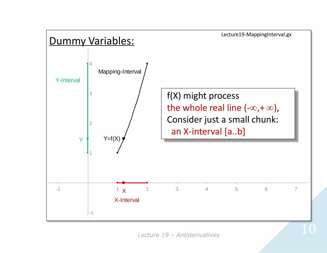
Dummy Variables:Lecture19-MappingInterval.gx

Consider a function f(X)that maps:an X-interval [a..b]

to a Y-interval [f(a)..f(b)]


1 2 3 4 5 6 7 8 9-1-2-3

1

2

3

4

5

6

-1

-2

1 2 3 4 5 6 7 8 9-1-2-3

1

2

3

4

5

6

-1

-2

X

Y=f(X)

X-Interval

Y-Interval

Y

Mapping-Interval


f(X) might processthe whole real line (-,+ ),Consider just a small chunk:an X-interval [a..b]

11

1 2 3 4 5 6 7 8 9-1-2-3

1

2

3

4

5

6

-1

-2

1 2 3 4 5 6 7 8 9-1-2-3

1

2

3

4

5

6

-1

-2

X

Y=f(X)

X-Interval

Y-Interval

Y

Mapping-Interval


When we compose g(f(x)),the interval that g() processesis notthe interval that f() processes.g() processes the output of f(),not the input x.


1 2 3 4 5 6 7 8 9-1-2-3

1

2

3

4

5

6

-1

-2

1 2 3 4 5 6 7 8 9-1-2-3

1

2

3

4

5

6

-1

-2

X

Y=f(X)

X-Interval

Y-Interval

Y

Mapping-Interval


As we work with antiderivatives we compose functions. You may hear the term “dummy variable”. When we have f=f(X) and g= g(X) we can reduce confusion by using different names for the domains of f and g. We might say that f=f(X) and g = f(U), so that when we compose f() and g() we understand that the output of one function is being used as the input of another.

13

1 2 3 4 5 6 7 8 9-1-2-3

1

2

3

4

5

6

-1

-2

1 2 3 4 5 6 7 8 9-1-2-3

1

2

3

4

5

6

-1

-2

X

Y=f(X)

X-Interval

Y-Interval

Y

Mapping-Interval

Domains & Ranges, Inputs & Outputs:Lecture19-MappingInterval.gx

Intervals on x are called the domain of f().Intervals on f(x) are called the range of f().The domain can be finite or infinite.The range can be finite or infinite.

Bounded on Lower & Upper

Lower Upper Neither

domain [a..b] [a..) (-..b] (-..+)

range [f(a)..f(b)] [f(a)..f(+)) (f(-)..f(b)] (f(-)..f(+))


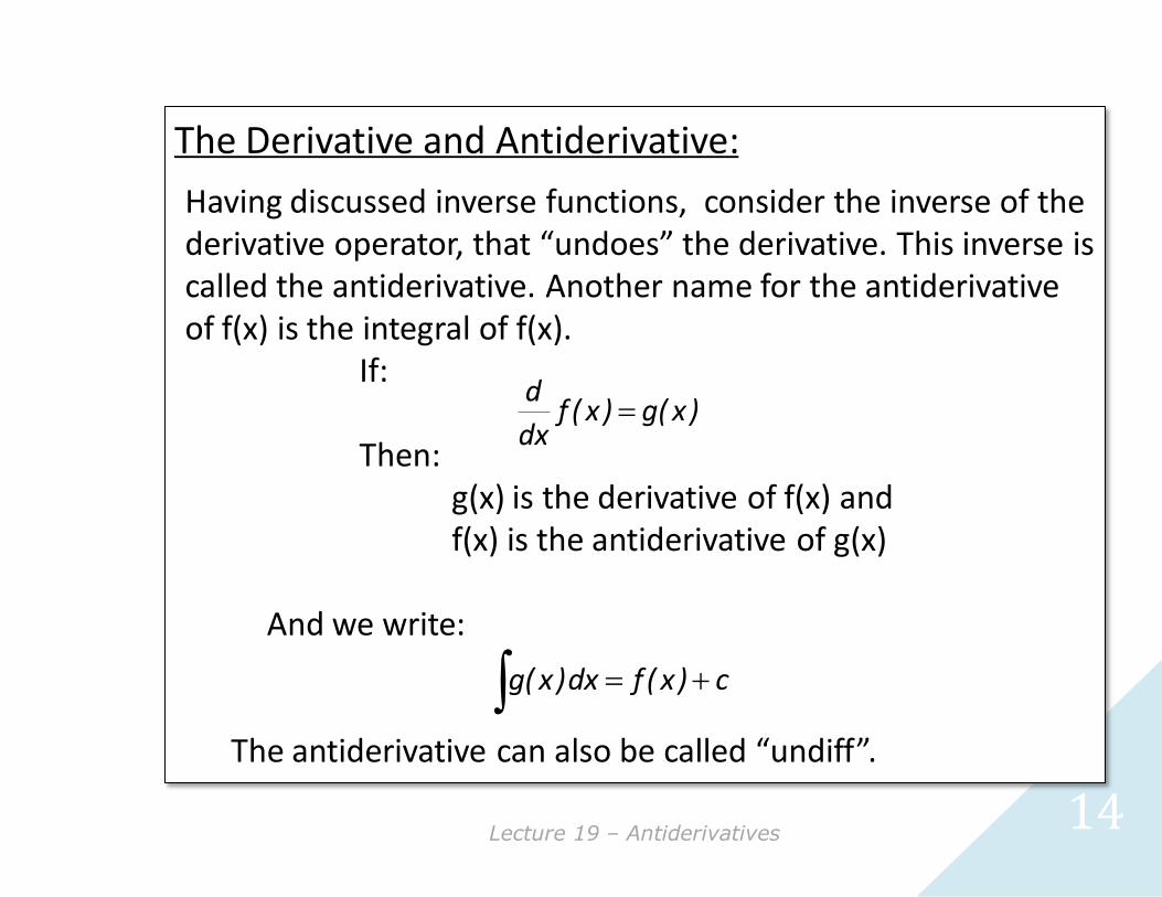
Having discussed inverse functions, consider the inverse of the derivative operator, that “undoes” the derivative. This inverse is called the antiderivative. Another name for the antiderivative of f(x) is the integral of f(x).

If:

Then:g(x) is the derivative of f(x) andf(x) is the antiderivative of g(x)

And we write:

The antiderivative can also be called “undiff”.

The Derivative and Antiderivative:

)x(g)x(fdx

d

c)x(fdx)x(g

15

Y=C+X3

C

Y=1+C+X3

Y=-1+C+X3

Y=X2

A Certain Antiderivative:Lecture19-ACertainAntiderivative.gx

Exercises:1) Open the example, drag point labeled C.2) Differentiate each green cubic function by hand.3) For large X, what values do the green functions have?4) Intersect the red function with each of its three antiderivative

functions, to discover three intersection points.

c3

XdXX

22


Previously we wrote the position of a falling object as:

Assuming “up” is positive, differentiating yields:

Differentiating again we are left like our friendhere with the acceleration due to gravity:

The minus sign reminds us that gravity pulls.

Differentiating in Reverse for Falling:

21y f (t ) gt

2

'dyf (t ) v gt

dt

2''

2

d yf (t ) a g

dt

-Li Wei

17

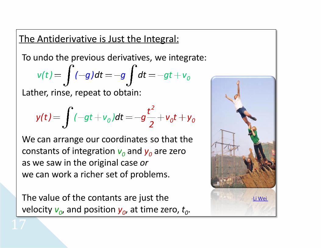
To undo the previous derivatives, we integrate:

Lather, rinse, repeat to obtain:

We can arrange our coordinates so that theconstants of integration v0 and y0 are zeroas we saw in the original case orwe can work a richer set of problems.

The value of the contants are just thevelocity v0, and position y0, at time zero, t0.

The Antiderivative is Just the Integral:

0( g)dtv(t ) gt vg dt

0

2

0 0dtt

y(t ) g v t y2

( gt v )

-Li Wei


The Falling Integral:Lecture19-Falling.gx

Exercise:1) Open the example, drag the two constants v0 and y0.2) Change the gravitational acceleration g to match:

the Moon (1.6 m/s), Earth (9.8 m/s) and Mars 3.7 (m/s).Add horizontal lines corresponding to these values of g.Note how sensitive the path of the object is to g.

3) The position of the object initially increases with time, why?4) Where does max-min theory appear in this example?

0

2

0 0dtt

y(t ) g v t y2

( gt v )

0( g)dtv(t ) gt vg dt

19

The Falling Integral: Symbolically

1) Integrate acceleration to obtain velocity.

2) Integrate velocity to obtain position.

3) Find the critical x value.

4) Find the critical y value.

Lecture19-Falling.wxm


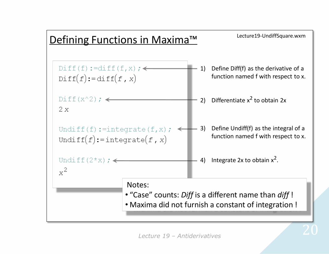
Defining Functions in Maxima™

1) Define Diff(f) as the derivative of a function named f with respect to x.

2) Differentiate x2 to obtain 2x

3) Define Undiff(f) as the integral of a function named f with respect to x.

4) Integrate 2x to obtain x2.

Lecture19-UndiffSquare.wxm

Notes:• “Case” counts: Diff is a different name than diff !• Maxima did not furnish a constant of integration !

21

We have used several notations for the same idea. We know:

We could just as well write:

and then take the antiderivative or “undiff” of both sides:

This is what we do with the integrate command in Maxima™.

Antiderivative as Undiff:

sin( x)d

cos( x)dx

sin( xDiff ( ) )) cos( x

Undiff ( sin( x) ) Undiff ( )

sin( x) Undiff (

Diff ( ) cos( x)

cos( x )

sin( x

)

co) x)ds( x


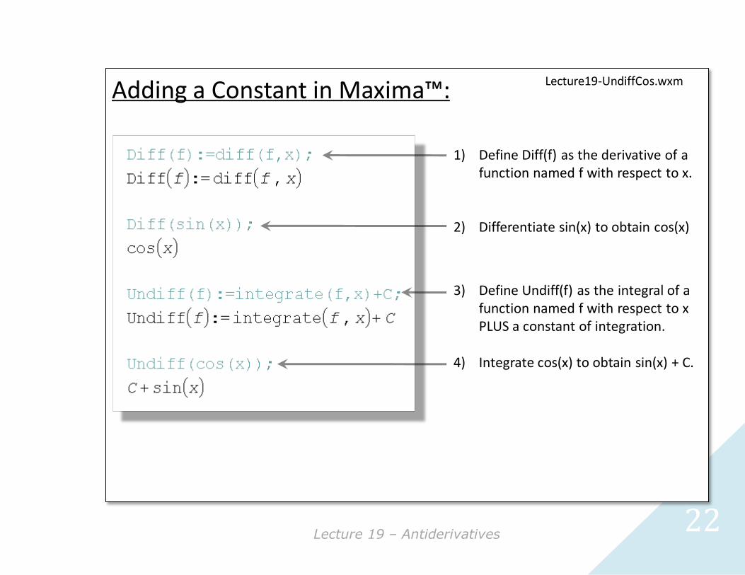
Adding a Constant in Maxima™:

1) Define Diff(f) as the derivative of a function named f with respect to x.

2) Differentiate sin(x) to obtain cos(x)

3) Define Undiff(f) as the integral of a function named f with respect to xPLUS a constant of integration.

4) Integrate cos(x) to obtain sin(x) + C.

Lecture19-UndiffCos.wxm

23

2 4 6 8-2-4-6-8

2

4

6

8

10

-2

2 4 6 8-2-4-6-8

2

4

6

8

10

-2

sin(t)+C

cos(t)

C

By adding the constant wepreserve the inverse.

Lecture19-UndiffCos.gx Diff Sine, Undiff Cosine in GX™:

Exercises:1) Open the example, drag point labeled C.2) Note that when we integrate we must

always introduce a constant of integration. dx sin( x) Ccos( x)


The power law states:

For the special case of n = 1 we have:

We can write this as:

And Undiff both sides:

The Antiderivative Power Law n = 1:

n n 1dn

xx x

d

1 11 0d1 x 1 x 1 1 1

dxx

Diff ( x) 1

Undiff ( x ) UndifDiff ( ) 1f ( ) x C

dx dx x C1

-Li Wei

25

For the case of n = 2 we have:




2 2 1 1d2 x 2 x 2xx

dx

2xDiff ( )x

2

2 2

2

x xUndiff ( ) Undiff ( ) C

2

Diff ( )x

2

xx

dx C2

-Li Wei


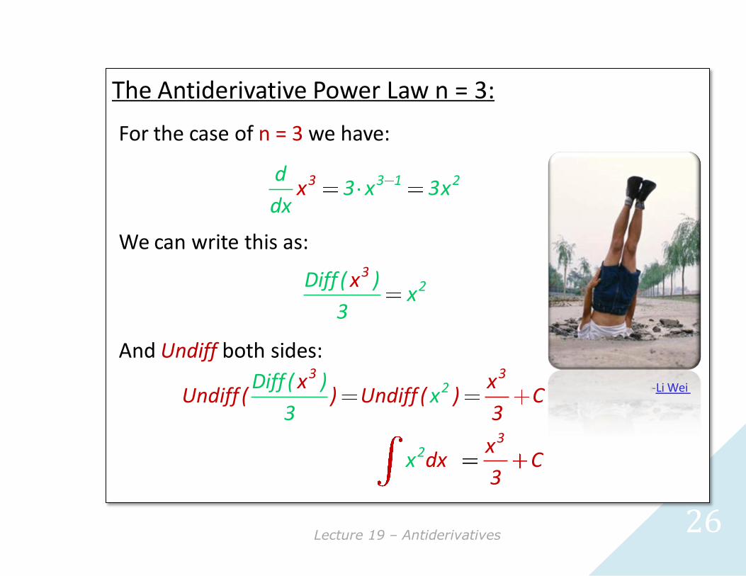
For the case of n = 3 we have:




3 3 1 2d3 x 3x

dxx

32Diff ( )

3

xx

3 3

3

2

2

x xUndiff ( ) Undif

Difff ( ) C

3

( )x

3

xx

dx C3

-Li Wei

27

1 2 3 4 5 6 7-1

1

2

3

4

5

1 2 3 4 5 6 7-1

1

2

3

4

5

Y=Xn

n

Y=X-1+n

·n

1/n

Lecture19-ACertainInverseSequel.gx

Exercise:1) Open the example, drag point labeled n.2) Notice the symmetry of n and 1/n.3) Are these functions inverses?4) If so, under what conditions?

A Certain Inverse, The Sequel:


End

cf ( x) c f ( x)

[ f ( x) g( x)]

dx dx

dx f ( x) g( x d)dx x

Y= X - wdv.com · example, f(x) = x , says that the function named f maps its input x to its output...

Documents

Transcript of Y= X - wdv.com · example, f(x) = x , says that the function named f maps its input x to its output...