S O C I A L A N D P S Y C H O L O G I C A L F A C T O R S A F F E C T I N G F E R T I L I T Y

XVI. FERTILITY RATES AND FERTILITY PLANNING BY CHARACTEROF MIGRATION1

J. F. K a n t n e r a n d P. K. W h e l p t o n

THIS study deals with some of the relationships between physical mobility and patterns of reproductive behavior. Specifically, frequency of movement is studied in rela­

tion to (a ) number of live births and (b ) the extent to which fertility is planned. In addition, the relationship of the size and location of the migrant’s community of origin to his fer­tility and fertility planning is investigated. Some attempt will also be made to deal with the interaction among these variables.

As formulated by the Committee2 the nature of these rela­tionships is not specified. Perhaps a fair amount of agreement could be obtained to the following statement:

Frequency of movement is inversely related to the size of planned families and directly related to the extent of fertility planning.8 [Hypothesis (a ) ]

In support of Hypothesis (a ) one might point to the secu­larizing effect of movement on such attitudinal systems as the “ large family ideal.” Or, approaching the matter somewhat differently, it appears that movement involves certain costs and that these vary directly with the frequency of movement. Other things equal, the restriction of family size and extent of planning would vary directly with the costs and therefore the

1 This is the sixteenth of a series of reports on a study conducted by the Com­mittee on Social and Psychological Factors Affecting Fertility, sponsored by the Milbank Memorial Fund with grants from the Carnegie Corporation of New York. The Committee consists of Lowell J. Reed, Chairman; Daniel Katz; E. Lowell Kelly; C. V. Kiser; Frank Lorimer; Frank W. Notestein; Frederick Osborn; S. A. Switzer; Warren S. Thompson; and P. K. Whelpton.

2 Hypothesis 11 of the list originally formulated by the Committee reads as fol­lows: The number, size, and location of communities in which couples have lived affect the proportion practicing contraception effectively and the size of planned families.

8 “ Planned families” and “extent of planning fertility” are explained in footnote 19.

153frequency of movement. Obviously the costs of movement are a function of factors besides frequency; both distance and dis­similarity of milieu are undoubtedly involved. To some extent all of these considerations are taken into account when number of moves and size of community or origin are cross tabulated.

The second part of this study investigates the relationship between (a ) the size and location of the migrant’s community of origin, and (b ) fertility and fertility planning. At least two inquiries could be followed up here: (1 ) How do birth rates and contraceptive practices of migrants differ from those of nonmigrants in the community of destination (Indianapolis)? Related to this is the question of how these behaviors vary within the group of migrants classified by size and location of community of origin. (2 ) How do the birth rates and contra­ceptive practices of migrants differ from those of nonmigrants in their communities of origin? For reasons discussed below this question cannot be satisfactorily answered in this study.

The first question, which can be investigated with present data, probes an area in which our knowledge is incomplete. Cities are commonly viewed as consumers and rural areas as suppliers of population. This circulation of population is vital to our scheme of organization. The fertility patterns of popu­lations at various points along the rural-urban continuum are well documented but the fertility patterns of those caught up in the population flow are less well known.4 In order to focus this part of the investigation two additional hypotheses are set up:

Planned families of urban migrants to Indianapolis are smaller in size than those of nonmigrants in Indianapolis. Planned families of rural migrants to Indianapolis are larger than those of Indianapolis nonmigrants. [Hypothesis (b -1 )] Urban migrants to Indianapolis are more effective in fertility planning than Indianapolis nonmigrants. Rural migrants to Indianapolis are less effective in fertility planning than In-

4 See Whelpton, P. K .: N eeded P opulation R esearch. The Science Press, Lan­caster, Pa. 1938. pp. 46-47.

Factors Affecting Fertility: Part X V I

dianapolis nonmigrants. [Hypothesis (b-2) ] In the formula­tion of Hypotheses (b-1) and (b-2) it is recognized that al­though transition between different environments may tend to depress fertility and encourage effective fertility planning this may not be sufficient to overcome the inertia of habit patterns acquired in the community of origin. Thus it is predicted that high fertility and ineffective fertility planning patterns devel­oped in the rural community will survive the migration process.

One additional hypothesis will be tested. This is: Within the migrant group, the size of the community in which couples lived before coming to Indianapolis is inversely related to the the size of planned families and directly related to the extent of fertility planning. [Hypothesis ( c ) ] Although Hypothesis (c ) may appear to be self evident, it is conceivable that it might not be true. For example, it is possible that the resist­ances to movement vary inversely with community size. Thus, it could be that what we might call the marginal encumbrance of children is greater in small than in large communities and leads to the selection of relatively unencumbered (small) fami­lies for migration from small communities.

P r e v io u s S t u d ie s o f t h e R e l a t io n s h ip B e t w e e n M o b il it y a n d F e r t i l i t y

Evidence from previous studies is not in full agreement with Hypothesis (a). Two studies yield a direct relationship, two an inverse relationship, and another no relationship between mobility and fertility. No study relating mobility and fertility planning was found in a survey of the literature. Manschke,5 using Swiss data for an earlier period, found that migrants gen­erally have higher fertility rates than nonmigrants. This is con­sistent with a positive correlation between mobility and num­ber of children found by Winkler.6

Two different studies made in Baltimore indicate an indirect5 Cited in Thomas, Dorothy Swaine: Research Memorandum on Migration Dif­

ferentials, (Bulletin 43) New York, Social Science Research Council, 1938, pp. 320-321.

6 Ibid. pp. 339-340.

154 The Milbank Memorial Fund Quarterly

155

relationship. Luykx7 shows that for both Negroes and Whites large families tended to be more permanent in the area studied than smaller families. Downes, Collins, and Jackson8 present data showing that the mean family size is greater for “ stable” than for “ mobile” families.

Edin9 found no relationship when a correction was made for the higher percentage of employed wives among the migrants.10

In general, the crude definitions of mobility, the apparent lack of controls for such relevant items as age, duration of mar­riage, ethnic composition, etc. as well as lack of agreement among these studies, justify further inquiry.

S iz e o f C o m m u n i t y o f O r ig in a n d F e r t i l i t y

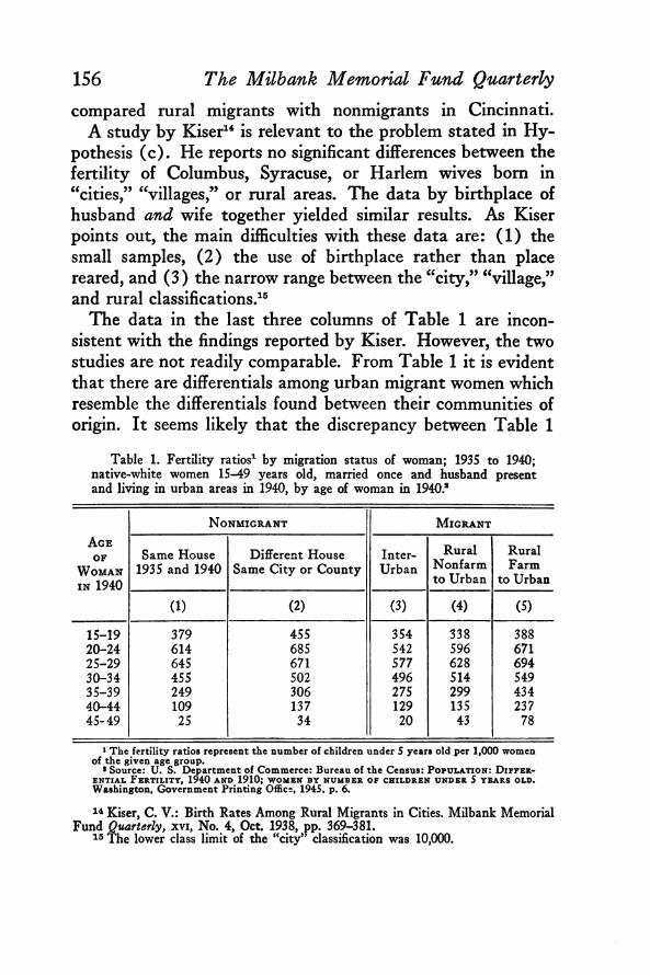
Data consistent with the argument in Hypothesis (b-1) may be found in the 1940 Census. Table 1 indicates that interurban migrants in 1940 had lower age-specific fertility ratios at ages under thirty11 than the more stable of the two groups of non­migrants (col. 1). The fertility ratios of interurban migrants were lower at all ages than were those of intra-urban “ mi­grants” (col. 2 ). The “ rural-farm to urban” migrants (col. 5) exhibited consistently higher fertility ratios than the more stable group of nonmigrants. The ratios of the “ rural-farm to urban” migrants were also higher than those of the intra-urban migrants except in the ages 15-24. This is consistent with studies by Feld12 who compared the rates of rural-born women in Zurich with Zurich-born women and by Leyboume13 who

7 Luykx, H. M. C.: Family Studies in the Eastern Health District, IV. Perma­nence of Residence with Respect to Various Family Characteristics, Human Biology, Vol. 19, No. 3, Sept. 1947, pp. 91-132.

8 Downes, Jean; Collins, Selwyn D.; and Jackson, Elizabeth H.: Characteristics of Stable and Non-Stable Families in the Morbidity Study in the Eastern Health District of Baltimore, Milbank Memorial Fund Quarterly, xxvn, No. 13, July 1949,pp. 260-282.

9 Thomas, op. cit. p. 92.10 This factor is not directly controlled in the present study but is perhaps par­

tially caught up in the control for socio-economic status.11 It is fairly well established that the years under thirty are the years of

greatest mobility so that the data in Table 1 may also support Hypothesis (a).12 Thomas, D. S.: op. cit. pp. 307-308.13 Leyboume, Grace G.: Urban Adjustments of Migrants from the Southern

Appalachian Plateaus, Social Forces, xvi, No. 4, Dec. 1937, pp. 238-247.

Factors Affecting Fertility: Part X V I

156compared rural migrants with nonmigrants in Cincinnati.

A study by Kiser14 is relevant to the problem stated in Hy­pothesis (c ) . He reports no significant differences between the fertility of Columbus, Syracuse, or Harlem wives bom in “ cities,” “ villages,” or rural areas. The data by birthplace of husband and wife together yielded similar results. As Kiser points out, the main difficulties with these data are: (1 ) the small samples, (2 ) the use of birthplace rather than place reared, and (3 ) the narrow range between the “ city,” “ village,” and rural classifications.15

The data in the last three columns of Table 1 are incon­sistent with the findings reported by Kiser. However, the two studies are not readily comparable. From Table 1 it is evident that there are differentials among urban migrant women which resemble the differentials found between their communities of origin. It seems likely that the discrepancy between Table 1

The Milbank Memorial Fund Quarterly

Table 1. Fertility ratios1 by migration status of woman; 1935 to 1940; native-white women 15-49 years old, married once and husband present and living in urban areas in 1940, by age of woman in 1940*

A ceof

W o m a n in 1940

N o n m ig r a n t M ig r a n t

Same House 1935 and 1940

Different House Same City or County

Inter-Urban

Rural Nonfarm to Urban

Rural Farm

to Urban

(1 ) (2 ) (3) (4) (S)

15-19 379 455 354 338 38820-24 614 685 542 596 67125-29 645 671 577 628 69430-34 455 502 496 514 54935-39 249 306 275 299 43440-44 109 137 129 135 23745-49 25 34 20 43 78

1 The fertility ratios represent the number of children under 5 years old per 1,000 women of the given age group.

* Source: U . S. Department of Commerce: Bureau of the Census: P o p u l a t io n : D if f e r ­e n t ia l F e r t il it y , 1940 a n d 1910; w o m e n b y n u m b e r o f c h il d r e n u n d e r 5 y e a r s o l d . Washington, Government Printing Office, 1945, p. 6.

14 Kiser, C. V.: Birth Rates Among Rural Migrants in Cities. Milbank Memorial Fund Quarterly, xvi, No. 4, Oct. 1938, pp. 369-381.

15 The lower class limit of the “ city” classification was 10,000.

and Kiser’s findings are explicable in terms of the relative re­moteness in time of the residential classifications.

Although the data from the 1940 Census are probably the best that have been available up to the present time, they leave unanswered certain questions. For example, we do not know how much mobility is associated with the various migrant clas­sifications since only two points in the woman’s migration his­tory are known, i.e. residence in 1935 and 1940. We do not know what differences in fertility might appear if classification were based on the husband’s migration status or on the joint migration status of husband and wife. On these matters the In­dianapolis data throw some light.16

T he Data

A detailed description of the methods of collecting data and the nature of the data has been given in previous reports in this series.17 All tabulations in this study are for “ relatively fecund” couples. The “ inflated” sample of 1,444 couples is used as the basis for all tabulations but the application of chi square takes

16 The chief superiority of the Census data is the possibility of making con­trolled comparisons between the rates of migrants and nonmigrants, urban against urban; rural-nonfarm against rural-nonfarm; rural-farm against rural-farm, even though the degree of control achieved is not great. The difficulties in the way of setting up outside control groups in the present study are discussed in the next section.

17 The following summary is repeated from an earlier study:Briefly stated, short schedules were filled out for 41,498 native-white couples

with wife under 45 in a Household Survey of Indianapolis. The Intensive Study was restricted to 2,589 native-white Protestant couples whose marriages were contracted during 1927-1929, and were unbroken at the time of the interview in 1941. Additional requirements for inclusion were: the wife was under 30 and the husband under 40 at marriage, neither had been previously married, the couple had resided in a large city most of the time since marriage, and both husband and wife had at least completed grammar school.

At the conclusion of the field work long schedules had been completed for 860 “ relatively fecund” couples and briefer ones for 220 “ relatively sterile” couples, a total of 1,080. The adjusted or “ inflated” sample consists of 1,444 “ relatively fecund” and 533 “ relatively sterile” couples, a total of 1,977. Couples refusing to cooperate in the Study comprise about 11 per cent of those contacted. Despite their absence, the inflated sample is quite similar to the original universe of 2,589 eligible couples not only with respect to the distribution by number of live births but also with respect to such distributions as dwelling units by rental value and husbands and wives by age and educational attainment.

Kiser, C. V. and Whelpton, P. K.: Social and Psychological Factors Affecting Fertility, IX Fertility Planning and Fertility Rates by Socio-Economic Status, Mil- bank Memorial Fund Quarterly, April, 1949, x x v ii , No. 2, p. 192. (Reprint p. 363.)

Factors Affecting Fertility: Part X V I 157

into account the fact that only 860 cases were independently drawn.18

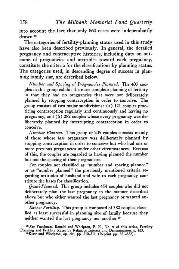
The categories of fertility-planning status used in this study have also been described previously. In general, the detailed pregnancy and contraceptive histories, including data on out­come of pregnancies and attitudes toward each pregnancy, constitute the criteria for the classifications by planning status. The categories used, in descending degree of success in plan­ning family size, are described below.

Number and Spacing of Pregnancies Planned. The 403 cou­ples in this group exhibit the most complete planning of fertility in that they had no pregnancies that were not deliberately planned by stopping contraception in order to conceive. The group consists of two major subdivisions: (a ) 121 couples prac­ticing contraception regularly and continuously and having no pregnancy, and (b ) 282 couples whose every pregnancy was de­liberately planned by interrupting contraception in order to conceive.

Number Planned. This group of 205 couples consists mainly of those whose last pregnancy was deliberately planned by stopping contraception in order to conceive but who had one or more previous pregnancies under other circumstances. Because of this, the couples are regarded as having planned the number but not the spacing of their pregnancies.

For couples not classified as “ number and spacing planned” or as “ number planned” the previously mentioned criteria re­garding attitudes of husband and wife to each pregnancy con­stitute the bases for classification.

Quasi-Planned. This group includes 454 couples who did not deliberately plan the last pregnancy in the manner described above but who either wanted the last pregnancy or wanted an­other pregnancy.

Excess Fertility. This group is composed of 382 couples classi­fied as least successful in planning size of family because they neither wanted the last pregnancy nor another.19

19 See Freedman, Ronald and Whelpton, P. K., No. x of this series, Fertility Planning and Fertility Rates by Religious Interest and Denomination, p. 423.

19Kiser and Whelpton, op. cit., pp. 210-211 (Reprint pp. 381-382).

158 The Milbank Memorial Fund Quarterly

159

Data relating to movement are available by number of moves for the ten years before marriage and the period since marriage. Only moves between communities are considered. Movement of husband and wife is tabulated separately for the premarital period.

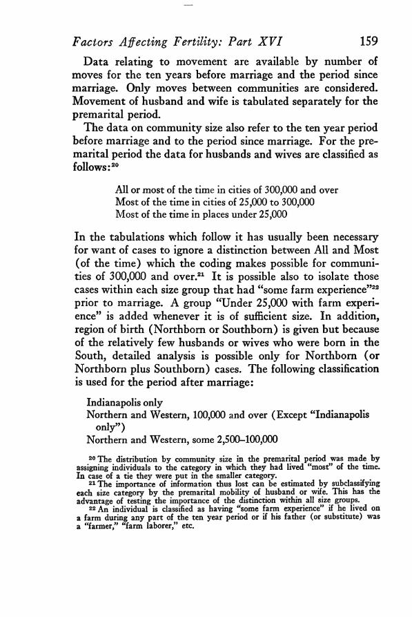
The data on community size also refer to the ten year period before marriage and to the period since marriage. For the pre­marital period the data for husbands and wives are classified as follows:20

All or most of the time in cities of 300,000 and over Most of the time in cities of 25,000 to 300,000 Most of the time in places under 25,000

In the tabulations which follow it has usually been necessary for want of cases to ignore a distinction between All and Most (of the time) which the coding makes possible for communi­ties of 300,000 and over.21 It is possible also to isolate those cases within each size group that had “ some farm experience”22 prior to marriage. A group “ Under 25,000 with farm experi­ence” is added whenever it is of sufficient size. In addition, region of birth (Northbom or Southbom) is given but because of the relatively few husbands or wives who were born in the South, detailed analysis is possible only for Northborn (or Northborn plus Southbom) cases. The following classification is used for the period after marriage:

Indianapolis onlyNorthern and Western, 100,000 and over (Except “ Indianapolis

only” )Northern and Western, some 2,500-100,000

20 The distribution by community size in the premarital period was made by assigning individuals to the category in which they had lived “most” of the time. In case of a tie they were put in the smaller category.

21 The importance of information thus lost can be estimated by subclassifying each size category by the premarital mobility of husband or wife. This has the advantage of testing the importance of the distinction within all size groups.

22 An individual is classified as having “some farm experience” if he lived on a farm during any part of the ten year period or if his father (or substitute) was a “farmer,” “ farm laborer,” etc.

Factors Affecting Fertility: Part X V I

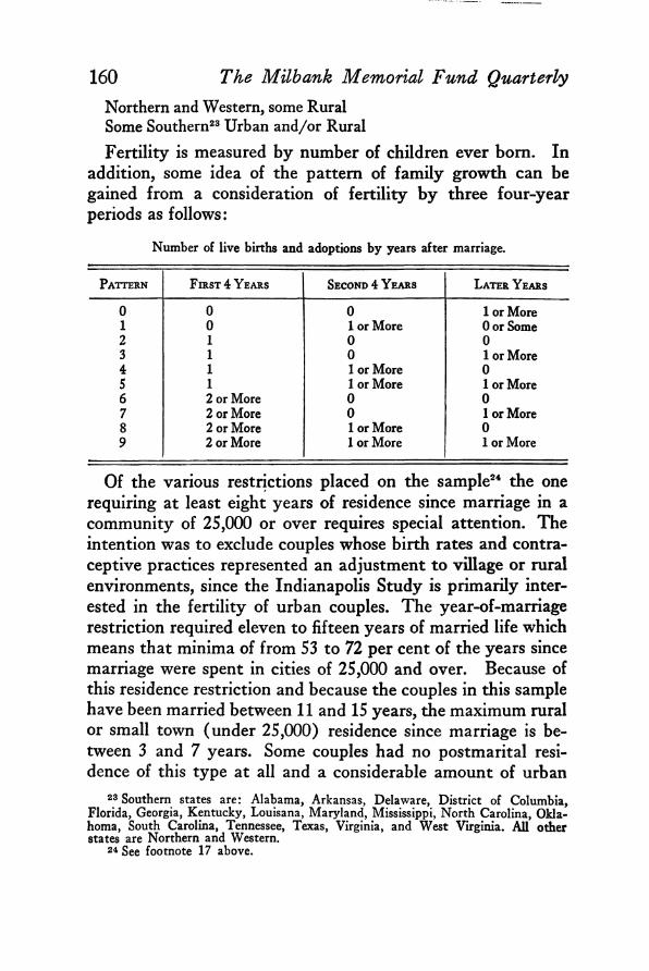
160Northern and Western, some RuralSome Southern23 Urban and/or RuralFertility is measured by number of children ever bom. In

addition, some idea of the pattern of family growth can be gained from a consideration of fertility by three four-year periods as follows:

The Milbank Memorial Fund Quarterly

Number of live births and adoptions by years after marriage.

Pattern F irst 4 Y ears Second 4 Y ears L ater Y ears

0 0 0 1 or More1 0 1 or More 0 or Some2 1 0 03 1 0 1 or More4 1 1 or More 0S 1 1 or More 1 or More6 2 or More 0 07 2 or More 0 1 or More8 2 or More 1 or More 09 2 or More 1 or More 1 or More

Of the various restrictions placed on the sample24 the one requiring at least eight years of residence since marriage in a community of 25,000 or over requires special attention. The intention was to exclude couples whose birth rates and contra­ceptive practices represented an adjustment to village or rural environments, since the Indianapolis Study is primarily inter­ested in the fertility of urban couples. The year-of-marriage restriction required eleven to fifteen years of married life which means that minima of from 53 to 72 per cent of the years since marriage were spent in cities of 25,000 and over. Because of this residence restriction and because the couples in this sample have been married between 11 and 15 years, the maximum rural or small town (under 25,000) residence since marriage is be­tween 3 and 7 years. Some couples had no postmarital resi­dence of this type at all and a considerable amount of urban

23 Southern states are: Alabama, Arkansas, Delaware, District of Columbia, Florida, Georgia, Kentucky, Louisana, Maryland, Mississippi, North Carolina, Okla­homa, South Carolina, Tennessee, Texas, Virginia, and West Virginia. All other states are Northern and Western.

24 See footnote 17 above.

161experience is characteristic of all categories. The likelihood is very great that this tends to reduce the size of the differences in fertility and fertility planning to be found when couples are classified by their postmarital residence.

The residence requirement undoubtedly has the effect also of reducing the size of the group having rural or village residence before marriage. The consequences of the restriction for pre­marital and postmarital mobility are less apparent.25

As suggested earlier in this paper, it is not possible to com­pare the fertility rates of migrant couples with those of non­migrant couples in the communities of origin. Even if data for nonmigrants were available there would be the difficulty that

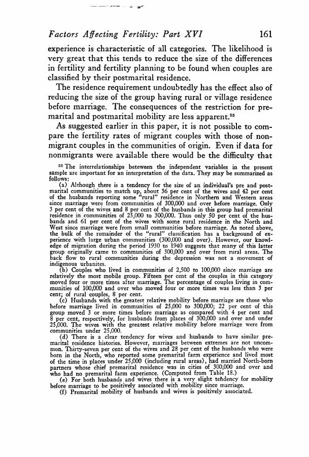
25 The interrelationships beteween the independent variables in the present sample are important for an interpretation of the data. They may be summarized as follows:

(a) Although there is a tendency for the size of an individual’s pre and post­marital communities to match up, about 36 per cent of the wives and 42 per cent of the husbands reporting some “rural” residence in Northern and Western areas since marriage were from communities of 300,000 and over before marriage. Only 3 per cent of the wives and 8 per cent of the husbands in this group had premarital residence in communities of 25,000 to 300,000. Thus only 50 per cent of the hus­bands and 61 per cent of the wives with some rural residence in the North and West since marriage were from small communities before marriage. As noted above, the bulk of the remainder of the “ rural” classification has a background of ex­perience with large urban communities (300,000 and over). However, our knowl­edge of migration during the period 1930 to 1940 suggests that many of this latter group originally came to communities of 300,000 and over from rural areas. The back flow to rural communities during the depression was not a movement of indigenous urbanites.

(b) Couples who lived in communities of 2,500 to 100,000 since marriage are relatively the most mobile group. Fifteen per cent of the couples in this category moved four or more times after marriage. The percentage of couples living in com­munities of 100,000 and over who moved four or more times was less than 3 per cent; of rural couples, 8 per cent.

(c) Husbands with the greatest relative mobility before marriage are those who before marriage lived in communities of 25,000 to 300,000; 22 per cent of this group moved 3 or more times before marriage as compared with 4 per cent and 8 per cent, respectively, for husbands from places of 300,000 and over and under 25,000. The wives with the greatest relative mobility before marriage were from communities under 25,000.

(d) There is a clear tendency for wives and husbands to have similar pre­marital residence histories. However, marriages between extremes are not uncom­mon. Thirty-seven per cent of the wives and 28 per cent of the husbands who were born in the North, who reported some premarital farm experience and lived most of the time in places under 25,000 (including rural areas), had married North-born partners whose chief premarital residence was in cities of 300,000 and over and who had no premarital farm experience. (Computed from Table 18.)

(e) For both husbands and wives there is a very slight tehdency for mobility before marriage to be positively associated with mobility since marriage.

(f) Premarital mobility of husbands and wives is positively associated.

Factors Affecting Fertility: Part X V I

162for the Indianapolis couples there tends to be an inverse rela­tionship between the age of the wife at the time of enumeration and the number of children ever bom. This results from the way in which age at marriage and duration of marriage were handled in the selection of the sample.26 Thus, simple age standardized rates do not provide a basis for comparison, and age and duration specific rates are not available for, say, the population of Indiana by appropriate population size groups.

But in spite of the fact that these data are in some ways not ideal for an investigation of the general relationship between migration and fertility, they are superior in several other ways to data available to previous investigators. Their advantages are: the provision of an improved measure of mobility (number of moves instead of migrant-nonmigrant status); information regarding migration in the premarital and postmarital periods; the possibility of dealing with mobility and community size jointly; the use of a better set of class intervals for community size; the ability to deal with fertility planning both as a control and as a dependent variable.

F in d in g s

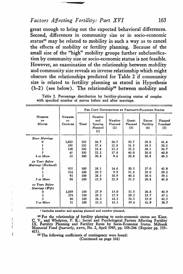
Hypothesis ( a)Number of Moves and Fertility-Planning Status. The data

in Table 2 do not indicate a relationship, either positive or nega­tive, between frequency of movement before or after marriage and fertility planning. The relationships in columns 1 to 4 for each section of the table were tested by chi square and found not to be significant. This lack of relationship is surprising in view of the importance attributed to mobility in sociological theory. Several post factum interpretations suggest them­selves.27 First, the range of differences in mobility may not be

Whelpton, P. K. and Kiser, C. V.: Social and Psychological Factors Affecting Fertility V. The Sampling Plan, Selection, and the Representativeness of Couples in the Inflated Sample. Milbank Memorial Fund Quarterly, xxiv, No. 1, Jan. 1946. pp. 88-90 (Reprint pp. 202-204).

27 That the negative findings reported in this paper may be a function of small numbers should be kept in mind constantly.

The Milbank Memorial Fund Quarterly

163

great enough to bring out the expected behavioral differences. Second, differences in community size or in socio-economic status28 may be related to mobility in such a way as to cancel the effects of mobility or fertility planning. Because of the small size of the “ high” mobility groups further subclassifica­tion by community size or socio-economic status is not feasible. However, an examination of the relationship between mobility and community size reveals an inverse relationship which might obscure the relationships predicted for Table 2 if community size is related to fertility planning as stated in Hypothesis (b-2) (see below). The relationship29 between mobility and

Table 2. Percentage distribution by fertility-planning status of couples with specified number of moves before and after marriage.

Factors Affecting Fertility: Part X V I

P e r C e n t D is t r ib u t io n b y F e r t il it y - P l a n n in g St a t u s

N u m b e r

o f

M o v e s

N u m b e r

o f

C o u p l e s Total

Numberand

SpacingPlanned

(1)

NumberPlanned

(2)

Quasi-Planned

(3)

ExcessFertility

(4)

PlannedFamilies1

(5)

S in ce M a rria ge0 1,023 100 26.7 14.7 30.7 28.0 41.41 195 100 37.4 12.8 31.3 18.5 50.22 128 100 23.4 13.3 35.2 28.1 36.73 45 100 22.2 17.8 40.0 20.0 40.0

4 or More 52 100 30.8 9.6 30.8 28.8 40.3i o Y ears B efore

M a rria g e (H u sb a n d )0 935 100 28.1 14.6 30.3 27.0 42.81 314 100 29.3 9.9 31.8 29.0 39.22 92 100 28.3 10.9 40.2 20.6 39.1

3 or More 96 100 22.9 22.9 33.3 20.8 45.8i o Y ea rs B e fo re M a rria g e ( W i fe )

0 1,059 100 27.9 13.0 32.3 26.8 40.91 274 100 29.2 17.9 29.2 23.7 47.12 80 100 26.2 16.2 32.5 25.0 42.5

3 or More 31 100 22.6 16.1 19.4 41.9 38.7

1 Includes number and spacing planned and number planned.

28 For the relationship of fertility planning to socio-economic status see Kiser, C. V., and Whelpton, P. K.: Social and Psychological Factors Affecting Fertility IX. Fertility Planning and Fertility Rates by Socio-Economic Status. Milbank Memorial Fund Quarterly, x x v ii , No. 2, April 1949, pp. 188-244 (Reprint pp. 359- 415).

29 The following coefficients of contingency were found:(Continued on page 164)

socio-economic status30 does not seem to be of sufficient mag- tude to cancel the relationship expected between mobility and fertility planning.

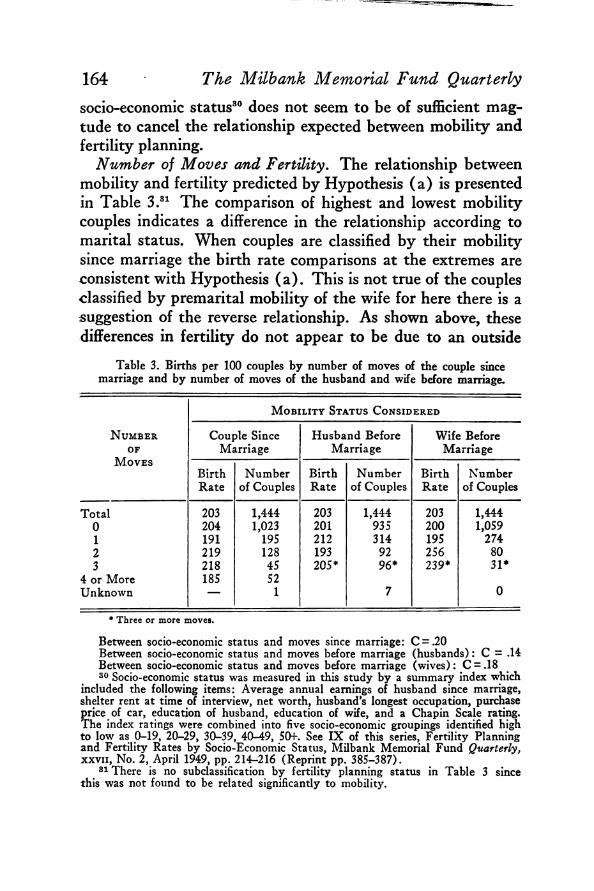
Number of Moves and Fertility. The relationship between mobility and fertility predicted by Hypothesis (a ) is presented in Table 3.31 The comparison of highest and lowest mobility couples indicates a difference in the relationship according to marital status. When couples are classified by their mobility since marriage the birth rate comparisons at the extremes are consistent with Hypothesis (a ). This is not true of the couples classified by premarital mobility of the wife for here there is a suggestion of the reverse relationship. As shown above, these differences in fertility do not appear to be due to an outside

Table 3. Births per 100 couples by number of moves of the couple since marriage and by number of moves of the husband and wife before marriage.

164 The Milbank Memorial Fund Quarterly

M o b il it y St a t u s C o n s id e r e d

N u m b e rOF

M o v e s

Couple Since Marriage

Husband Before Marriage

Wife Before Marriage

BirthRate

Number of Couples

BirthRate

Number of Couples

BirthRate

Number of Couples

Total 203 1,444 203 1,444 203 1,4440 204 1,023 201 935 200 1,0591 191 195 212 314 195 2742 219 128 193 92 256 803 218 45 205* 96* 239* 31*

4 or More 185 52Unknown — 1 7 0

* Three or more moves.

Between socio-economic status and moves since marriage: C = .20 Between socio-economic status and moves before marriage (husbands): C = .14 Between socio-economic status and moves before marriage (wives): C = .18 30 Socio-economic status was measured in this study by a summary index which

included the following items: Average annual earnings of husband since marriage, shelter rent at time of interview, net worth, husband’s longest occupation, purchase price of car, education of husband, education of wife, and a Chapin Scale rating. The index ratings were combined into five socio-economic groupings identified high to low as 0-19, 20-29, 30-39, 40-49, SOf. See IX of this series, Fertility Planning and Fertility Rates by Socio-Economic Status, Milbank Memorial Fund Quarterly, x x v ii , No. 2, April 1949, pp. 214-216 (Reprint pp. 385-387).

81 There is no subclassification by fertility planning status in Table 3 since this was not found to be related significantly to mobility.

Factors Affecting Fertility: Part X V I 165

N u m b e r of M o ves of t h e H u sb a n d

N u m b e r of M o v e s of t h e W if e

0 1 2 or More

BirthRate

Number of Couples

BirthRate

Number of Couples

BirthRate

Number of Couples

0 201 724 201 211 193 1211 187 160 204 80 209 32

2 or More 241 51 335 23 214 35

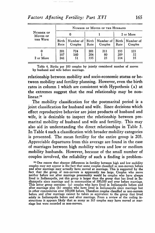
Table 4. Births per 100 couples by jointly considered number of moves by husband and wife before marriage.

relationship between mobility and socio-economic status or be­tween mobility and fertility planning. However, even the birth rates in column 1 which are consistent with Hypothesis (a ) at the extremes suggest that the real relationship may be non­linear.32

The mobility classification for the postmarital period is a joint classification for husband and wife. Since decisions which effect reproductive behavior are joint products of husband and wife, it is desirable to inspect the relationship between pre­marital mobility of husband and wife and fertility. This may also aid in understanding the direct relationships in Table 3. In Table 4 such a classification with broader mobility categories is presented. The mean fertility for the entire group is 203. Appreciable departures from this average are found in the case of marriages between high mobility wives and low or medium mobility husbands. However, because of the small number of couples involved, the reliability of such a finding is problem-

32 One reason that sharper differences in fertility between high and low mobility couples may not appear is the fact that some couples classified as non-movers before and after marriage may actually have moved at marriage. This is suggested by the fact that the group of non-movers is apparently too large. Couples who move neither before nor after marriage presumably would be couples who have always lived in Indianapolis, yet this group is larger than the group that has lived in In­dianapolis since marriage and in communities of 300,000 and over before marriage. This latter group contains: (a) couples who have lived in Indianapolis before and after marriage plus (b) couples who have lived in Indianapolis since marriage but in other communities over 300,000 before. Therefore couples classified as non-movers before and after marriage cannot be taken as equivalent to the group that lived solely in Indianapolis before and after marriage. From a review of the coding in­structions it appears likely that as many as 163 couples may have moved at mar­riage but were recorded as non-movers.

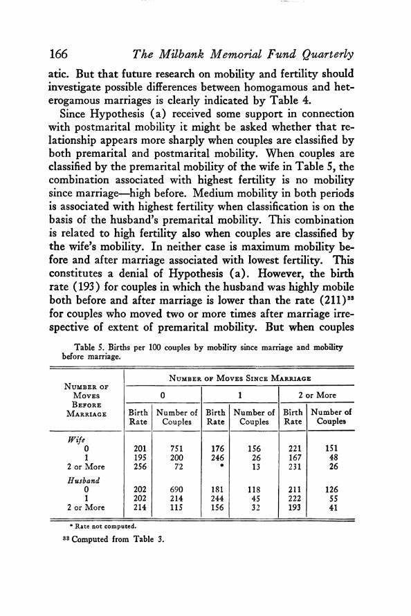
166atic. But that future research on mobility and fertility should investigate possible differences between homogamous and het- erogamous marriages is clearly indicated by Table 4.

Since Hypothesis (a ) received some support in connection with postmarital mobility it might be asked whether that re­lationship appears more sharply when couples are classified by both premarital and postmarital mobility. When couples are classified by the premarital mobility of the wife in Table 5, the combination associated with highest fertility is no mobility since marriage—high before. Medium mobility in both periods is associated with highest fertility when classification is on the basis of the husband’s premarital mobility. This combination is related to high fertility also when couples are classified by the wife’s mobility. In neither case is maximum mobility be­fore and after marriage associated with lowest fertility. This constitutes a denial of Hypothesis (a ). However, the birth rate (193 ) for couples in which the husband was highly mobile both before and after marriage is lower than the rate (211)ss for couples who moved two or more times after marriage irre­spective of extent of premarital mobility. But when couples

The Milbank Memorial Fund Quarterly

Table 5. Births per 100 couples by mobility since marriage and mobility before marriage.

N u m b e r of M o ves B e f o r e

M a r r ia g e

N u m b e r of M o v e s Sin c e M a r r ia g e

0 1 2 or More

BirthRate

Number of Couples

BirthRate

Number of Couples

BirthRate

Number of Couples

Wife0 201 751 176 156 221 1511 195 200 246 26 167 48

2 or More 256 72 ♦ 13 231 26Husband

0 202 690 181 118 211 1261 202 214 244 45 222 SS

2 or More 214 115 156 32 193 41

* Rate not computed.

33 Computed from Table 3.

Factors Affecting Fertility: Part X V I 167

P a t t e r n o f F a m il y G r o w t h N u m b e r of M o v e s S in c e M a r r ia g e

PatternNumber

Number of Births Occurring Within Successive Four-Year

Periods of Married Life 0 1 2 34 or

More

FirstPeriod

SecondPeriod

ThirdPeriod

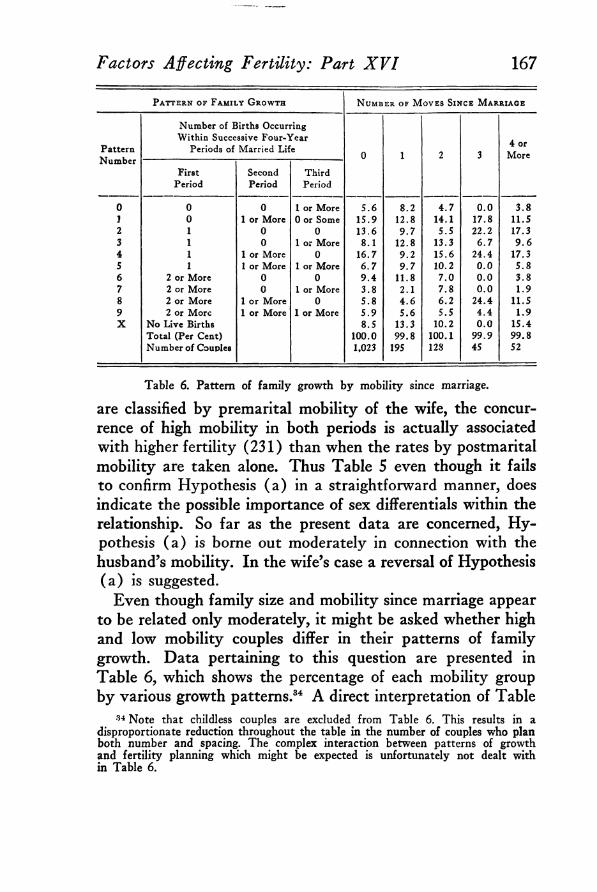
0 0 0 1 or More 5.6 8.2 4.7 0.0 3.81 0 I or More 0 or Some 15.9 12.8 14.1 17.8 11.52 1 0 0 13.6 9.7 5.5 22.2 17.33 1 0 1 or More 8.1 12.8 13.3 6.7 9 .64 1 1 or More 0 16.7 9.2 15.6 24.4 17.35 1 1 or More 1 or More 6.7 9.7 10.2 0.0 5.86 2 or More 0 0 9.4 11.8 7.0 0.0 3.87 2 or More 0 1 or More 3.8 2.1 7.8 0.0 1.98 2 or More 1 or More 0 5.8 4.6 6.2 24.4 11.59 2 or More 1 or More 1 or More 5.9 5.6 5.5 4.4 1.9X No Live Births 8.5 13.3 10.2 0.0 15.4

Total (Per Cent) 100.0 99.8 100.1 99.9 99.8Number of Couples 1,023 195 128 45 52

Table 6. Pattern of family growth by mobility since marriage.

are classified by premarital mobility of the wife, the concur­rence of high mobility in both periods is actually associated with higher fertility (231) than when the rates by postmarital mobility are taken alone. Thus Table 5 even though it fails to confirm Hypothesis (a ) in a straightforward manner, does indicate the possible importance of sex differentials within the relationship. So far as the present data are concerned, Hy­pothesis (a ) is borne out moderately in connection with the husband’s mobility. In the wife’s case a reversal of Hypothesis (a ) is suggested.

Even though family size and mobility since marriage appear to be related only moderately, it might be asked whether high and low mobility couples differ in their patterns of family growth. Data pertaining to this question are presented in Table 6, which shows the percentage of each mobility group by various growth patterns.34 A direct interpretation of Table

34 Note that childless couples are excluded from Table 6. This results in a disproportionate reduction throughout the table in the number of couples who plan both number and spacing. The complex interaction between patterns of growth and fertility planning which might be expected is unfortunately not dealt with in Table 6.

1686 is made difficult by the fact that family size is not controlled. Thus the relatively greater occurrence of non-movers than of high mobility couples in pattern 9 may be a function of the larger families of the former group. This difficulty can be over­come to some extent by comparing pairs of patterns— 3 and 4,7 and 8—in which size of family may be fairly similar. An­other difficulty is that we do not know in which period since marriage the migrations occurred. On the basis of general knowledge we might expect a tendency for movement to be con­centrated in the first four years after marriage. The way in which this general tendency may have been modified by the conditions affecting this group of migrants in the years 1930 to 1934 is difficult to estimate. It is nevertheless of interest to look for differences in family growth patterns between high and low mobility couples.

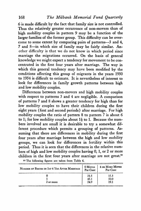
Differences between non-movers and high mobility couples with respect to patterns 3 and 4 are negligible. A comparison of patterns 7 and 8 shows a greater tendency for high than for low mobility couples to have their children during the first eight years (first and second periods) after marriage. For high mobility couples the ratio of pattern 8 to pattern 7 is about 6 to 1; for low mobility couples about H to 1. Because the num­bers involved are small it is desirable to try a somewhat dif­ferent procedure which permits a grouping of patterns. As­suming that there are differences in mobility during the first four years after marriage between the high and low mobility groups, we can look for differences in fertility within this period. Thus it is seen that the differences in the relative num­bers of high and low mobility couples having 0, 1, or 2 or more children in the first four years after marriage are not great.35

The Milbank Memorial Fund Quarterly

35 The following figures are taken from Table 6.

N um ber of B irths in 1st 4 Y rs A fter M arriage0 M oves Per Cent

4 or M ore M oves Per Cent

0 21.5 15.31 45.1 50.02 or more 24.9 19.1

169Factors Affecting Fertility: Part X V I

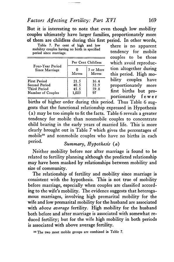
But it is interesting to note that even though low mobility couples ultimately have larger families, proportionately more of them are childless during this first period. In other words,

Table 7. Per cent of high and low mobility couples having no birth in specified period since marriage.

there is no apparent tendency for mobilecouples to be those which avoid reproduc­tion altogether during this period. High mo­bility couples have proportionately more first births but pro-

_______________ portionately f e w e rbirths of higher order during this period. Thus Table 6 sug­gests that the functional relationship expressed in Hypothesis (a ) may be too simple to fit the facts. Table 6 reveals a greater tendency for mobile than nonmobile couples to concentrate child bearing in the early years of married life. This is more clearly brought out in Table 7 which gives the percentages of mobile36 and nonmobile couples who have no births in eachperiod. Summary, Hypothesis (a)

Four-Year Period Since Marriage

Per Cent Childless

0Moves

3 or More Moves

First Period 21.5 16.4Second Period 40.5 32.9Third Period 45.5 59.8Number of Couples 1,023 97

Neither mobility before nor after marriage is found to be related to fertility planning although the predicted relationship may have been masked by relationships between mobility and size of community.

The relationship of fertility and mobility since marriage is consistent with the hypothesis. This is not true of mobility before marriage, especially when couples are classified accord­ing to the wife’s mobility. The evidence suggests that heteroga- mous marriages, involving high premarital mobility for the wife and low premarital mobility for the husband are associated with above average fertility. High mobility for the husband both before and after marriage is associated with somewhat re­duced fertility; but for the wife high mobility in both periods is associated with above average fertility.

36 The two most mobile groups are combined in Table 7.

Some differences are found in pattern of family growth be­tween high and low mobility couples. High mobility couples do not appear to reduce their fertility rates in the early periods of married life as much as do low mobility couples. To the extent that these early years are the years of greatest mobility this finding is inconsistent with Hypothesis (a ). However, pattern of family growth does not appear to be a simple linear function of mobility.

The fact that Hypothesis (a ) receives only qualified sub­stantiation from this analysis may be due in part to the rather high degree of homogeneity of the sample, one aspect of which is a limited range of mobility. However, the importance given to mobility in sociological theory would lead one to expect it to produce differences in behavior even among a fairly homo­geneous group. Perhaps the most important implication of this analysis of Hypothesis (a ) is the question it raises concerning the sufficiency of the concept of mobility in sociological gen­eralizations.

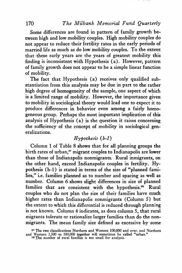
Hypothesis ( b-1)Column 1 of Table 8 shows that for all planning groups the

birth rates of urban,37 migrant couples to Indianapolis are lower than those of Indianapolis nonmigrants. Rural inmigrants, on the other hand, exceed Indianapolis couples in fertility. Hy­pothesis (b-1) is stated in terms of the size of “ planned fami­lies,” i.e. families planned as to number and spacing as well as number. Column 6 shows slight differences in size of planned families that are consistent with the hypothesis.88 Rural couples who do not plan the size of their families have much higher rates than Indianapolis nonmigrants (Column 5) but the extent to which this differential is reduced through planning is not known. Column 4 indicates, as does column 5, that rural migrants tolerate or rationalize larger families than do the non­migrants. The mean family size defined as excessive by some

87 The two classifications Northern and Western 100,000 and over, and Northern and Western 2,500 to 100,000 together will sometimes be called “ urban.”

38 The number of rural families is too small for analysis.

170 The Milbank Memorial Fund Quarterly

171nonmigrants is 44 per cent greater than the family size “ ac­cepted” by other nonmigrants whereas the comparable figure for rural migrants is 56 per cent. If it is assumed that this same relative difference persists between Quasi-planned and Planned Families, an “ estimated” rate of rural Planned Families may be computed. This rate is shown in column 6. The rates of migrant and nonmigrant couples in column 6 are consistent with Hypothesis (b-1) but perhaps the more important obser­vation is the relative convergence of rates among Planned Families in contrast to the spread in columns 4 and 5.

An investigation of Hypothesis (b-1) with respect to resi-

Factors Affecting Fertility: Part X V I

Table 8. Births per 100 couples by fertility-planning status and by residence since marriage.

F e r t il it y - P l a n n in g S t a t u s

C o m m u n it y S iz e All NumberNumberPlanned

Quasi-Planned

PlannedFamilies*a n d L o c a t io n Planning

Groups(1)

andSpacing

ExcessFertility

Planned(2)

(3) (4) (5) (6)

BIRTHS PER 100 COUPLES

Indianapolis Only Northern and Western,

204 110 229 199 286 152

100,000 and Over 184 104 * 203 • 140Northern and Western, Some

2,500-100,000 Northern and Western,

185 109 200 194 287 138

Some Rural 279 • • 242 377 169bNorthern Urban and Rural Some Southern Urban and

203 * * * * 140

Rural 192 * • • • 126

NUMBER OF COUPLES

Indianapolis Only Northern and Western

1,023 273 150 314 286 423

100,000 and Over 110 46 17 32 15 63Northern and Western, Some

2,500-100,000 Northern and Western,

179 55 26 67 31 81

Some Rural 72 13 4 24 31 17Northern Urban and Rural Some Southern Urban and

361 114 47 123 77 161

Rural 59 15 8 17 19 23

* Rate not computed.* Includes number and spacing planned and number planned. b Rate estimated. Procedure described in text.

dence before marriage was not undertaken for the following reasons: (a ) the analysis would not be especially meaningful if postmarital residence were not controlled, (b ) the only post- marital residential classification of sufficient size to withstand subclassification is “ Indianapolis Only,” and (c ) this would re­quire the isolation of couples who lived in Indianapolis before and after marriage as the nonmigrant group. However, (d ) as discussed in footnote 32, this group cannot be satisfactorily identified.

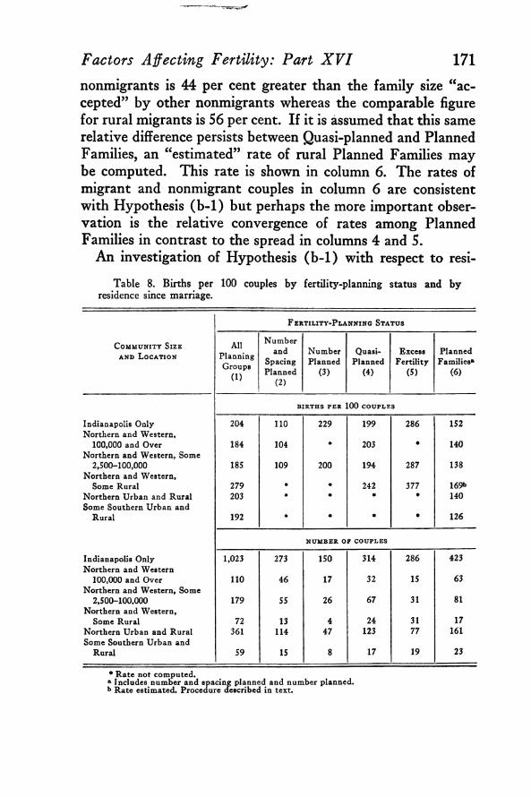
Although a migrant-nonmigrant comparison by community size for the premarital period cannot be made, we can still

;examine the relationship between postmarital migrant and nonmigrant couples subclassified by premarital residence. The data for all planning groups are presented in Table 9; subclas­sification by fertility planning status is not feasible. Nonmi-

172 The Milbank Memorial Fund Quarterly

Table 9. Births per 100 couples by residence before and after marriage.

C o m m u n it y S iz e S in c e M a r r ia g e

C o m m u n it y S iz e B e f o r e M a r r ia g e

Husband Wife

300,000. or Over

25,000-300,000

Under25,0001

Under 25,000

With Farm Experience

300,000 or Over

25,000-300,000

Under25,000*

Under 25,000

With Farm Experience

BIRTHS PER 100 COUPLES

Indianapolis Only 210 226 182 200 209 204 193 198Northern and Western, K\1

100,000 and Over 160 194* • • 128 190 227 •Northern and Western, -

Some 2,500-100,000 184 175 ^ 195 157 208 179 170 190Northern and Western,

Some Rural * • • 238 315 • 268 •

N U M B E R OF COUPLES

Indianapolis Only 592 27 98 121 586 28 122 132Northern and Western,

100,000 and Over 35 32 19 15 42 20 22 14Northern and Western,

Some 2,500-100,000 44 44 49 21 39 39 56 29Northern and Western,

Some Rural 19 3 15 21 20 2 22 19

1 Without farm experience. • Rate not computed.

173

grants since marriage classified by husband’s premarital resi­dence generally have higher fertility rates than urban migrants. Couples with some rural residence since marriage and in which the husband was rural before marriage have higher rates than nonmigrant couples in which the husband was rural before marriage. When couples are classified according to the wife’s premarital residence, the nonmigrant couples also tend to have higher rates than urban migrants and lower rates than rural migrants.

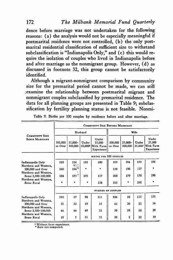
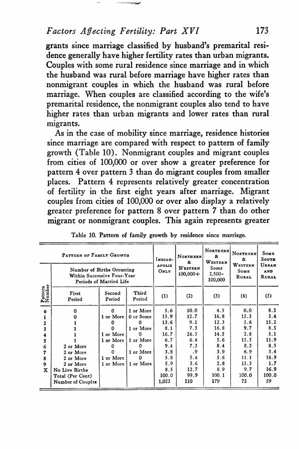
As in the case of mobility since marriage, residence histories since marriage are compared with respect to pattern of family growth (Table 10). Nonmigrant couples and migrant couples from cities of 100,000 or over show a greater preference for pattern 4 over pattern 3 than do migrant couples from smaller places. Pattern 4 represents relatively greater concentration of fertility in the first eight years after marriage. Migrant couples from cities of 100,000 or over also display a relatively greater preference for pattern 8 over pattern 7 than do other migrant or nonmigrant couples. This again represents greater

Factors Affecting Fertility: Part X V I

Table 10. Pattern of family growth by residence since marriage.

P a t t e r n o f F a m il y G r o w t hI n d ia n ­a p o l is

O n l y

N o r t h e r n

&W e s t e r n

10 0 ,00 0+

N o r t h e r n

&W e s t e r n

Some2,5 00 -100,000

N o r t h e r n

&W e s t e r n

S o m e

R u r a l

S o m e

S o u t h

U r b a n

a n d

R u r a l

Pat

tern

Num

ber

N um ber o f Births Occurring W ithin Successive F our-Y ear

Periods o f M arried Life

FirstPeriod

SecondP eriod

ThirdPeriod (1) (2) (3) (4 ) (5 )

0 0 0 1 or M ore 5 .6 10 .0 4 .5 0.0 8 .51 0 1 or M ore 0 or Some 1 5 .9 12 .7 16 .8 15.3 3 .42 1 0 0 1 3 .6 9 .1 12.3 5 .6 15 .23 1 0 1 or M ore 8 .1 7 .3 16 .8 9 .7 8 .54 1 1 or M ore 0 16 .7 24 .5 14.5 2 .8 5 .15 1 1 or M ore 1 or M ore 6 .7 6 .4 5 .6 15.3 1 1 .96 2 or M ore 0 0 9 .4 7 .3 8 .4 8 .3 8 .57 2 or M ore 0 1 or M ore 3 .8 .9 3 .9 6 .9 3 .48 2 or M ore 1 or M ore 0 5 .8 5 .4 5 .6 11.1 16 .99 2 or M ore 1 or M ore 1 or M ore 5 .9 3 .6 2 .8 15.3 1 .7X N o L ive Births 8 .5 12 .7 8 .9 9 .7 16 .9

T ota l (P er C ent) 100.0 9 9 .9 100.1 100 .0 100 .0N um ber o f Couples 1,023 110 179 72 59

concentration of reproduction in early years of married life. Apart from this tendency for residents of larger cities to spread their fertility over a shorter time span, other differences in Table 10 appear to be a function of family size.

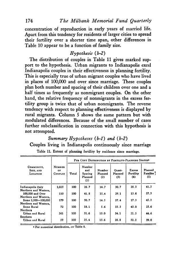
Hypothesis ( b-2)The distribution of couples in Table 11 gives marked sup­

port to the hypothesis. Urban migrants to Indianapolis excel Indianapolis couples in their effectiveness in planning fertility. This is especially true of urban migrant couples who have lived in places of 100,000 and over since marriage. These couples plan both number and spacing of their children over one and a half times as frequently as nonmigrant couples. On the other hand, the relative frequency of nonmigrants in the excess fer­tility group is twice that of urban nonmigrants. The reverse tendency with respect to planning effectiveness is displayed by rural migrants. Column 5 shows the same pattern but with modulated differences. Because of the small number of cases further subclassification in connection with this hypothesis is not attempted.

Summary Hypotheses ( b-1) and (b-2)Couples living in Indianapolis continuously since marriage

174 The Milbank Memorial Fund Quarterly

Table 11. Extent of planning fertility by residence since marriage.

P e r C e n t D is t r ib u t io n b y F e r t il it y - P l a n n in g S t a t u s*

C o m m u n it y , S iz e , a n d L o c a t io n

N u m b e r

OFC o u p l e s T ota l

N um berand

SpacingPlanned

(1 )

N um berPlanned

(2 )

Quasi-Planned

(3 )

ExcessFertility

(4)

Planned Families ^

(S)

Indianapolis Only N orthern and W estern,

1,023 100 2 6 .7 1 4 .7 3 0 .7 28 .3 41 .3

100,000 and Over N orthern and W estern,

110 100 4 1 .8 1 5 .4 29 .1 1 3 .6 57 .3

Som e 2,500— 100,000 N orthern and W estern,

179 100 3 0 .7 14 .5 3 7 .4 17 .3 45 .2

Some Rural N orthern

72 100 18 .1 5 .6 3 3 .3 4 3 .0 23 .6

Urban and Rural Southern

361 100 3 1 .6 1 3 .0 34 .1 21 .3 4 4 .6

Urban and Rural 59 100 2 5 .4 1 3 .6 2 8 .8 3 2 .2 39 .0

* For numerical distribution, see Table 8.

175

have larger planned families and are somewhat less effective planners than urban migrants to Indianapolis. The birth rate for planned families with some rural residence after marriage had to be estimated and in so far as the estimate has any value it indicates that rural couples since marriage have larger planned families than Indianapolis nonmigrants. These rural couples are less effective with respect to fertility planning than Indianapolis couples.

Wherever comparisons can be made, similar differences in fertility between nonmigrants and the urban and rural mi­grants are observable when their premarital residence history is taken into account.

Some differences in patterns of family growth are apparent. Urban migrants from large places tend to complete their re­productive life earlier than other groups. This cannot be ex­plained simply by their greater planning effectiveness which enables them to avoid pregnancy in the later periods of married life, because the pregnancy avoidance of other groups in the earlier periods of married life must also be explained. It is possible that the fertility planning status classification, which relies heavily on the attitude toward the last pregnancy for its definition of ineffectiveness, may not be realistic. This problem needs further exploration.

Hypothesis (b-1) cannot be tested adequately within socio­economic groups because of the small number of medium and high status couples with rural residence after marriage. Within the two lowest socio-economic categories, however, the data are consistent with the hypothesis. Among couples of medium and high status the birth rates of nonmigrants, and urban mi­grants are fairly similar. Medium status urban migrants have a rate of childlessness that is twice that of nonmigrants of like status. This is consistent with the hypothesis.

Hypothesis (c )The findings with respect to Hypothesis (c ) have already

been indirectly presented. Obviously, if urban migrants have

Factors Affecting Fertility: Part X V I

176 The Milbank Memorial Fund Quarterly

C o m m un ity , P er C ent D istribution by F er tility -P l a n n in g Status

Size , andTotal Number and Number Quasi- Excess

L ocation Spacing Planned Planned Planned Fertility

high status

North and West Cities:

100,000 and Over 100 44.1 13.6 37.3 5.12,500— 100,000 100 39.5 15.1 26.8 18.6Some Rural — — — — —

MEDIUM STATUS

North and West Cities:

100,000 and Over 100 53.8 26.9 15.4 3.82,500— 100,000 100 19.0 11.9 54.8 14.3Some Rural — — — — —

LOW STATUS

North and West Cities:

100,000 and Over 100 24.0 8.0 24.0 44.02,500— 100,000 100 25.5 15.7 41.2 17.6Some Rural 100 5.8 9.5 21.0 66.7

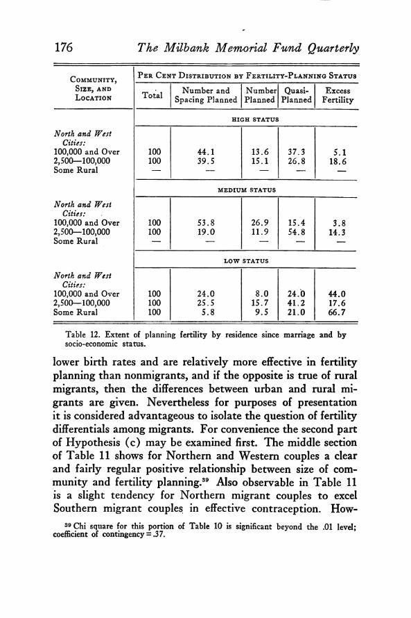
Table 12. Extent of planning fertility by residence since marriage and by socio-economic status.

lower birth rates and are relatively more effective in fertility planning than nonmigrants, and if the opposite is true of rural migrants, then the differences between urban and rural mi­grants are given. Nevertheless for purposes of presentation it is considered advantageous to isolate the question of fertility differentials among migrants. For convenience the second part of Hypothesis (c ) may be examined first. The middle section of Table 11 shows for Northern and Western couples a dear and fairly regular positive relationship between size of com­munity and fertility planning.89 Also observable in Table 11 is a slight tendency for Northern migrant couples to excel Southern migrant couples in effective contraception. How-

39 Chi square for this portion of Table 10 is significant beyond the .01 level; coefficient of contingency = .37.

177

ever, these differences are not great and cannot be analyzed further without knowledge of the internal, rural-urban, com­position of the two regional categories.

Table 12 tests the relationship between residence since mar­riage and fertility planning within socio-economic status cate­gories. In general, the relationship stands up within the three socio-econpmic groups.40 This is most apparent if the extreme planning status groups within each socio-economic level are considered. Differences consistent with Hypothesis (c ) appear in comparisons between places of 100,000 and over and places of 2,500 to 100,000 for high and medium socio-economic status

Factors Affecting Fertility: Part X V I

Table 13. Extent of planning fertility by residence of wife before marriage.

P e r C e n t D is t r ib u t io n b y F e r t il it y - P l a n n in g St a t u s

C o m m u n it y , S i z e , a n d L o c a t io n

N u m b e r

OFC o u p l e s T ota l

N um berand

SpacingPlanned

(1 )

N um berPlanned

(2 )

Quasi-Planned

(3 )

ExcessFertility

(4)

PlannedFam ilies

(5 )

Northborn and Southborn

300,000 and Over1 756 100 28 .1 1 3 .6 3 0 .6 2 7 .8 4 1 .725,000-300,0001 107 100 33 .3 14 .7 23 .3 2 8 .7 4 8 .0Under 25,000' 258 100 2 6 .2 15 .1 3 5 .0 2 3 .7 4 1 .3Under 25,000 with

Farm Experience 242 100 2 3 .0 1 5 .4 32 .2 29 .3 3 8 .4

N orthborn1300,000 and Over 704 100 2 8 .4 13 .3 2 9 .9 28 .3 4 1 .825,000-300,000 92 100 3 7 .0 13 .9 2 5 .0 24 .1 5 0 .9Under 25,000 223 100 26 .5 14 .1 35 .2 2 4 .2 4 0 .6

N orthborn ( W ith F a rm E xperien ce)

300,000 and Over 48 100 4 7 .9 6 .2 2 2 .9 2 2 .9 5 4 .125,000-300,000 0 — — — — — —Under 25,000 203 100 2 2 .2 16 .2 3 3 .0 2 8 .6 3 8 .4

Southborn300,000 and Over1 52 100 2 7 .6 15 .5 3 9 .7 17 .2 4 3 .125,000-300,000' 15 100 14 .3 1 9 .0 14 .3 5 2 .4 33 .3Under 25,000' 35 100 2 3 .9 21 .1 33 .8 21 .1 4 5 .0U nder 25,000 with

Farm Experience 3 9 100 2 7 .8 11 .1 2 7 .8 33 .3 3 8 .9

1 W ithout farm experience.

40 High = 0-19, 20-29; Medium = 30-39; Low = 40-49, 50 and over. For a de­scription of this socio-economic index see footnote 30 above.

groups. For low status couples the hypothesis is confirmed only in comparisons between rural places and cities of 100,000 and over. Chi square is significant only for the differences within the medium status group.41

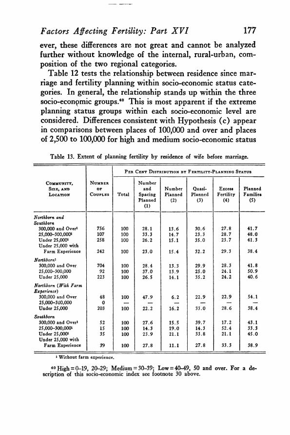
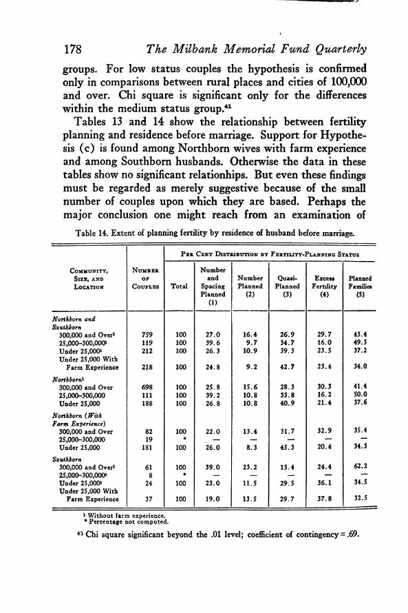
Tables 13 and 14 show the relationship between fertility planning and residence before marriage. Support for Hypothe­sis (c ) is found among Northbom wives with farm experience and among Southbom husbands. Otherwise the data in these tables show no significant relationhips. But even these findings must be regarded as merely suggestive because of the small number of couples upon which they are based. Perhaps the major conclusion one might reach from an examination of

178 The Milbank Memorial Fund Quarterly

Table 14. Extent of planning fertility by residence of husband before marriage.

P e r C e n t D is t r ib u t io n b y F e r t il it y - P l a n n in g St a t u s

C o m m u n it y , S i z e , a n d L o c a t io n

N u m b e r

o p

C o u p l e s T ota l

N um berand

SpacingPlanned

(1)

N um berPlanned

(2 )

Quasi-Planned

(3 )

ExcessFertility

(4 )

PlannedFamilies

(S)

N o rth b o m and S ou th bom

300,000 and Over1 759 100 2 7 .0 1 6 .4 2 6 .9 2 9 .7 43 .425,000-300,000' 119 100 3 9 .6 9 .7 3 4 .7 1 6 .0 49.3U nder 25,000 ' 212 100 2 6 .3 1 0 .9 3 9 .3 2 3 .5 37.2U nder 25,000 W ith

Farm Experience 218 100 2 4 .8 9 .2 4 2 .7 2 3 .4 34 .0

N o rth b o m 1300,000 and Over 698 100 2 5 .8 1 5 .6 2 8 .3 30 .3 41 .425,000-300,000 111 100 3 9 .2 1 0 .8 3 3 .8 16 .2 50 .0U nder 25,000 188 100 2 6 .8 1 0 .8 4 0 .9 2 1 .4 37.6

N o rth b o m ( W ith F a rm E xp erien ce)

35.4300,000 and Over 82 100 2 2 .0 1 3 .4 3 1 .7 3 2 .925,000-300,000 19 * — — — — —U nder 25,000 181 100 2 6 .0 8 .3 4 5 .3 2 0 .4 34.3

S ou th bom300,000 and Over1 61 100 3 9 .0 2 3 .2 1 3 .4 2 4 .4 62 .225,000-300,000' 8 • — — — — —Under 25,000' 24 100 2 3 .0 11 .5 2 9 .5 3 6 .1 34.5U nder 25,000 W ith

Farm Experience 37 100 1 9 .0 13 .5 2 9 .7 3 7 .8 32.5

1 W ithout farm experience.* Percentage not com puted.

41 Chi square significant beyond the .01 level; coefficient of contingency = .69.

179

Tables 11, 13, and 14 is that with respect to fertility planning, the postmarital environment appears to be of greater impor­tance than the premarital environment. It may be that the findings for Northborn wives with farm experience and South- bom husbands are interpretable in terms of the postmarital environment they represent.

Data bearing on the first part of Hypothesis (c ) are pre­sented in Table 8. There is virtually no difference between the birth rates of migrant couples, All Planning Groups, who lived in cities of 100,000 and over and those who lived in cities of 2,500 to 100,000 after marriage. However, there is a sharp birth rate differential between these urban migrants and those having some rural experience after marriage. The relationship cannot be tested among Planned Families because of the small number with rural experience.

A comparison of the rates for Northern and Southern couples indicates that regional differences are not great. The rates of Northern couples are slightly higher regardless of planning status. The relative contributions of urban and rural com­ponents to this result are not known.

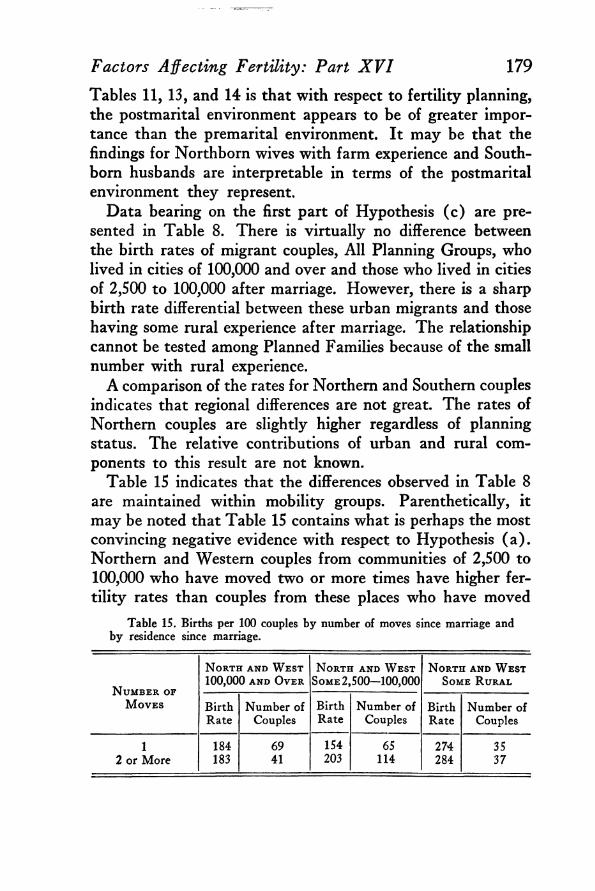
Table 15 indicates that the differences observed in Table 8 are maintained within mobility groups. Parenthetically, it may be noted that Table 15 contains what is perhaps the most convincing negative evidence with respect to Hypothesis (a ). Northern and Western couples from communities of 2,500 to100,000 who have moved two or more times have higher fer­tility rates than couples from these places who have moved

Factors Affecting Fertility: Part X V I

Table IS. Births per 100 couples by number of moves since marriage and by residence since marriage.

N u m b e r of M o v e s

N o r t h a n d W e st 100,000 a n d O v e r

N o r t h a n d W e st S om e 2,500— 100,000

N o r th a n d W e st So m e R u r a l

BirthRate

Number of Couples

BirthRate

Number of Couples

BirthRate

Number of Couples

12 or More

184183

6941

154203

65114

274284

3537

180only once. If Hypothesis (a ) were to hold anywhere it should be within this group since, as already pointed out, this popula­tion size group has the greatest relative representation in the high mobility categories.

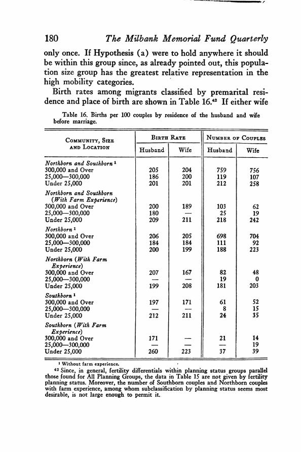
Birth rates among migrants classified by premarital resi­dence and place of birth are shown in Table 16.42 If either wife

The Milbank Memorial Fund Quarterly

Table 16. Births per 100 couples by residence of the husband and wife before marriage.

C om m u n ity , SizeB irth R at e N u m ber of C ouples

an d L ocation Husband Wife Husband Wife

Northborn and Southborn1300,000 and Over 205 204 759 75625,000— 300,000 186 200 119 107Under 25,000 201 201 212 258Northborn and Southborn

( With Farm Experience)300,000 and Over 200 189 103 6225,000— 300,000 180 — 25 19Under 25,000 209 211 218 242Northborn 1300,000 and Over 206 205 698 70425,000— 300,000 184 184 111 92Under 25,000 200 199 188 223Northborn (With Farm

Experience)300,000 and Over 207 167 82 4825,000— 300,000 — — 19 0Under 25,000 199 208 181 203Southborn 1300,000 and Over 197 171 61 5225,000— 300,000 — — 8 15Under 25,000 212 211 24 35Southborn (With Farm

Experience)300,000 and Over 171 — 21 1425,000— 300,000 — — — 19Under 25,000 260 223 37 39

1 Without farm experience.42 Since, in general, fertility differentials within planning status groups parallel

those found for All Planning Groups, the data in Table 15 are not given by fertility planning status. Moreover, the number of Southborn couples and Northborn couples with farm experience, among whom subclassification by planning status seems most desirable, is not large enough to permit it.

181

or husband was bom in the South or if the Northborn wife has had some farm experience, there is an inverse relationship between birth rates and community size before marriage. This seems to be the consequence both of below average rates among the most urban couples in these two groups and higher than average rates among the rural couples. That these rates are related to differences in contraceptive effectiveness is evident if one refers again to Tables 13 and 14. Beyond this however, it is not possible to go with the present data. Clearly here is an area needing further inquiry.

Also noteworthy in Table 16 is the fact that, in contrast to the wife, the fertility of Northborn husbands does not appear to be influenced by their contact with rural life. It is possible of course that under the rather broad definition being em­ployed, the type of “ farm experience” may differ between hus­bands and wives. The interpretation made of Table 16 should also take account of the possibility that in those cases where high fertility is associated with the classification “Under25,000 with Farm Experience” it may not be farm experience per se which is important but the selection of smaller com­munities under 25,000 which results from the combination with farm experience.

Factors Affecting Fertility: Part X V I

Table 17. Births per 100 couples living in Indianapolis since marriage by residence before marriage and by socio-economic status.

I n d e x of Socio-E conomic Status

R esidence B efore M arr iag e 0-19(High) 20-29 30-39 40-49

50 and Over (Low)

BIRTHS PER 100 COUPLES

Husband—Northborn and Southborn 300,000 and Over 182 153 134 196 309Under 25,000 and Rural 154 145 193 192 284Wife— Northborn and Southborn 300,000 and Over 178 164 190 196 303Under 25,000 and Rural 162 131 170 187 307

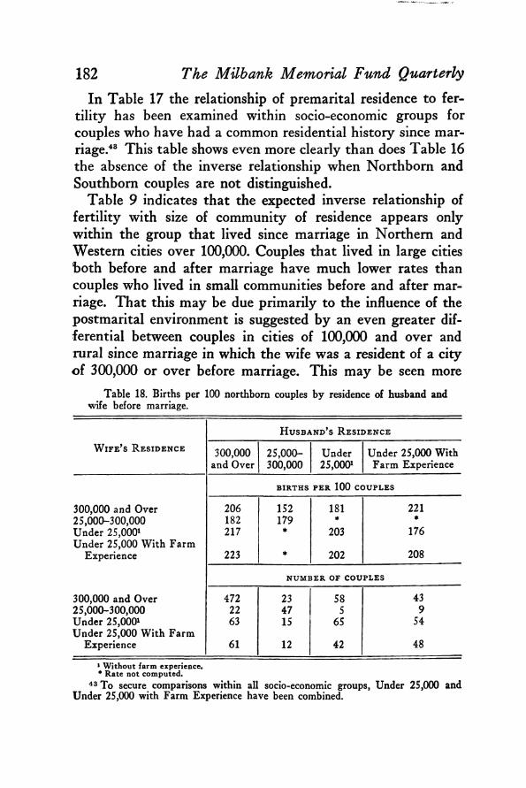
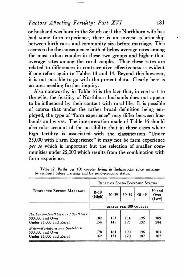
182In Table 17 the relationship of premarital residence to fer­

tility has been examined within socio-economic groups for couples who have had a common residential history since mar­riage.48 This table shows even more clearly than does Table 16 the absence of the inverse relationship when Northborn and Southbom couples are not distinguished.

Table 9 indicates that the expected inverse relationship of fertility with size of community of residence appears only within the group that lived since marriage in Northern and Western cities over 100,000. Couples that lived in large cities both before and after marriage have much lower rates than couples who lived in small communities before and after mar­riage. That this may be due primarily to the influence of the postmarital environment is suggested by an even greater dif­ferential between couples in cities of 100,000 and over and rural since marriage in which the wife was a resident of a city o f 300,000 or over before marriage. This may be seen more

The Milbank Memorial Fund Quarterly

Table 18. Births per 100 northborn couples by residence of husband and wife before marriage.

W ife ’ s R esidence

H u sban d ’s R esidence

300,000 and Over

25,000-300,000

Under25,000*

Under 25,000 With Farm Experience

BIRTHS PER 100 COUPLES

300,000 and Over 206 152 181 2212S,000-300,000 182 179 ♦ *Under 2S.0001 217 * 203 176Under 25,000 With Farm

Experience 223 * 202 208

n u m b er of couples

300,000 and Over 472 23 58 4325,000-300,000 22 47 5 9Under 25,000* 63 15 65 54Under 25,000 With Farm

Experience 61 12 42 48

1 W ithout farm experience.* R ate not com puted.

43 To secure comparisons within all socio-economic groups, Under 25,000 and Under 25,000 with Farm Experience have been combined.

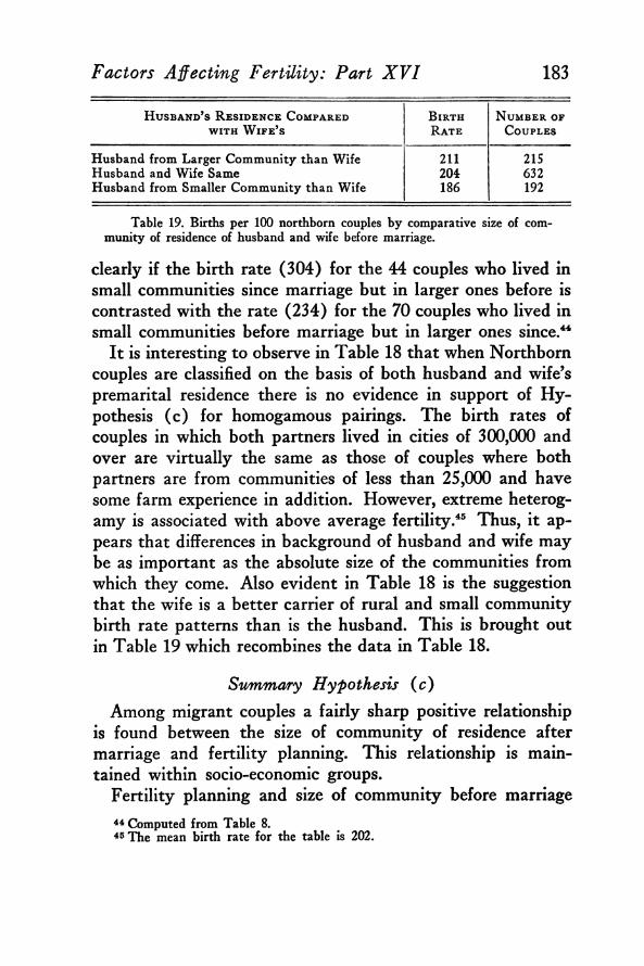
Factors Affecting Fertility: Part X V I 183

H usban d ’ s R esid ence C ompared B irth N um ber ofw it h W if e ’ s R ate C ouples

Husband from Larger Community than Wife 211 215Husband and Wife Same 204 632Husband from Smaller Community than Wife 186 192

Table 19. Births per 100 northborn couples by comparative size of com­munity of residence of husband and wife before marriage.

clearly if the birth rate (304) for the 44 couples who lived in small communities since marriage but in larger ones before is contrasted with the rate (234) for the 70 couples who lived in small communities before marriage but in larger ones since.4*

It is interesting to observe in Table 18 that when Northborn couples are classified on the basis of both husband and wife’s premarital residence there is no evidence in support of Hy­pothesis (c ) for homogamous pairings. The birth rates of couples in which both partners lived in cities of 300,000 and over are virtually the same as those of couples where both partners are from communities of less than 25,000 and have some farm experience in addition. However, extreme heterog- amy is associated with above average fertility.45 Thus, it ap­pears that differences in background of husband and wife may be as important as the absolute size of the communities from which they come. Also evident in Table 18 is the suggestion that the wife is a better carrier of rural and small community birth rate patterns than is the husband. This is brought out in Table 19 which recombines the data in Table 18.

Summary Hypothesis (c )Among migrant couples a fairly sharp positive relationship

is found between the size of community of residence after marriage and fertility planning. This relationship is main­tained within socio-economic groups.

Fertility planning and size of community before marriage44 Computed from Table 8.45 The mean birth rate for the table is 202.

are not positively related except among Northbom wives with farm experience and among Southbom husbands. (Tables 13- 14.) The existence of the relationship among Northbom wives with farm experience and among Southbom husbands seems to be due to the relatively high effectiveness of planning that results when these backgrounds are combined with residence before marriage in communities of 300,000 and over. It seems reasonable that these combinations represent a greater range of experience48 than any of the others and if so, the association with enhanced fertility planning is consistent with the argu­ment underlying the hypothesis. This argument, it will be re­called, stresses a positive relationship between degree of en­vironmental difference or, subjectively stated, range of new experience and tendency to plan. Presumably narrower ranges of experience before marriage are not sufficient to influence sub­sequent fertility planning. The suggestion that the postmarital environment is more important than the premarital environ­ment with respect to fertility planning is offered, although dif­ferences in the classifications make such a generalization haz­ardous.

An inverse relationship between family size and size of com­munity is found for the period since marriage. Whether this relationship is found among planned families cannot be deter­mined directly but it does appear when an estimated rate for rural couples is used.

Couples in which the husband or wife was bom in the South show an inverse relationship between fertility and size of com­munity before marriage. In the husband’s case this seems to be due to the high fertility of Southbom husbands from places under 25,000 and having some farm experience. In the wife’s case the relationship appears to result from low fertility among Southbom wives from places of 300,000 and over. Thus it may be that the social and psychological dynamics associated with being born (and perhaps reared) in the South are different for

46 Or perhaps greater adversity.

184 The Mtibank Memorial Fund Quarterly

185males and females. Further analysis is prevented by the small number of Southborn cases. This applies also to testing the relationhip with respect to the size of planned families.

Northborn wives with farm experience also show an inverse relationship between fertility and size of community before marriage. The low birth rates of the wives in this group who are from communities of 300,000 and over seem to be respon­sible for the relationship. It will be recalled that over 50 per cent of this group planned the number of children they had. The comparable husbands have higher birth rates. This dif­ference in response to a large urban environment might be due to substantive differences in the specification “ farm experi­ence” between males and females. Or it might represent a dif­ference in postmarital experience of males and females. It does not appear to be attributable to the fact that females are su­perior “ carriers” of rural behavior patterns.

When postmarital residence is controlled an inverse relation­ship between fertility and size of community before marriage appears only within the group that has lived in places of 100,000 and over since marriage. This relationship does not depend upon region of birth or upon having “ farm experience.” It is attributable both to low fertility among couples who have large city experience before and after marriage, and to rela­tively high fertility among couples who have small town or rural experience before marriage. The relationship is more pro­nounced for the wife. Like many of the findings reported in this paper, this one needs further investigation with a larger sample. Otherwise, the size of the community of residence be­fore marriage seems to be less closely associated with fertility than size of the community since marriage. Couples who lived in large communities before marriage and in small ones after­ward have higher birth rates than those who lived in large ones after and small ones before. However, this should be viewed with caution since “ small” places are not necessarily defined the same way in the two periods.

Finally it appears that combinations of large and small com-

Factors Affecting Fertility: Part X V I

186munity experience for husband and wife leads to greatest de­partures from average fertility. Extreme heterogamy in this respect is associated with highest fertility. In addition, the husband appears to be a less effective carrier of small com­munity birth rates than the wife. This may have something to do with known sex differences in migration. The longer dis­tances traveled by male migrants may entail greater uprooting than in the case of female migrants. This interpretation is con­sistent with the basic argument of the hypothesis but cannot be readily checked with the present data.

C o n c l u s io n

The data available from the Indianapolis study are not ideal for the investigation of the foregoing hypotheses. Small num­bers make some of the findings unreliable. Yet the examina­tion of the data has pointed up certain areas of critical inquiry and has indicated that the original hypotheses are sometimes oversimplified. Since the Indianapolis study was conceived as a pilot study by the Committee it is pertinent to conclude this paper with a list of problems to which special attention might be given in future studies. Therefore in addition to reexamin­ing all of the relationships of this study with a larger and per­haps less homogeneous sample, the following queries are sug­gested for consideration:

1. What is the critical range for mobility with respect to fer­tility and fertility planning? The present study indicates that neither fertility nor fertility planning is closely associated with variations in mobility within the range considered.

2. What differences in group structure are there between mar­riages of high mobility wives and low mobility husbands that are associated with higher fertility than either homoganous situation (i.e. low mobility for wife and husband or high mobility for both wife and husband ) ?

3. Similarly, what differences in group structure are there be­tween marriages that are homogamous and those that are hetero- gamous with respect to premarital residence?

The Milbank Memorial Fund Quarterly

4. What is relevant to fertility and fertility planning in the designation “ Southborn” ?

5. What is relevant to fertility and fertility planning in the designation “Northbom with farm experience” ? What sex differ­ences are there with respect to this background characteristic?

6. What would be the relationship of mobility or community size to fertility if couples were classified by postmarital experi­ence and premarital experience of husband and wife?

Other and perhaps more fruitful queries may occur to the reader.

Factors Affecting Fertility: Part X V I 187