XSophe, a Computer Simulation Software Suite

for the Analysis of

Electron Paramagnetic Resonance Spectra.

M. Griffin, A. Muys, C. Noble, D. Wang, C. Eldershaw,1a,b 1b 1b 1b 1a

K. E. Gates, K. Burrage and G. R. Hanson, 1a 1a 1b†

Department of Mathematics and Centre for Magnetic Resonance,1a 1b

The University of Queensland, St. Lucia, Queensland, Australia, 4072.

Author to whom correspondence should be addressed.†

Dr. Graeme HansonCentre for Magnetic ResonanceThe University of QueenslandSt. Lucia, Qld., Australia, 4072.Email address: Graeme.Hanson@CMR.uq.edu.auPh: +61-7-3365-3242Fax: +61-7-3365-3833

2

ABSTRACT

The XSophe computer simulation software suite consisting of a daemon, the XSophe interface

and the computational program Sophe is a state of the art package for electron paramagnetic

resonance simulation. The Sophe program performs the computer simulation and includes a number

of new technologies including; the SOPHE partition and interpolation schemes, a field segmentation

algorithm, homotopy, parallelisation and spectral optimisation. The SOPHE partition and

interpolation scheme along with a field segmentation algorithm greatly increases the speed of

simulations for most systems. The multidimensional homotopy provides an efficient method for

accurately tracing energy levels and hence tracing transitions in the presence of energy level

anticrossings and looping transitions and allowing computer simulations in frequency space. For

complex systems the parallelisation enables the simulation of these systems on a parallel computer

and the optimisation algorithms in the suite provide the experimentalist with the possibili ty of finding

the spin Hamiltonian parameters in a systematic manner rather than a trial-and-error process.

3

Keywords:

Electron Paramagnetic Resonance

Computer Simulation

Homotopy

Electron Spin Resonance

Spectral Optimisation

�A � S � D � S � � B � g � S � S � A � I � I � Q � I � � I (1 � ) � B

Total � � N

i � 1

�Ai � �

N

i , j � 1 , j � i

�Ai j

�Ai j � JAi j

SAi � SAj � dAi jSAi

× SAj � SAi � DAi j � SAj

4

(1)

(2)

1. Introduction

Multifrequency electron paramagnetic resonance (EPR) spectroscopy [1-7] is a powerful tool

for characterising paramagnetic molecules or centres within molecules that contain one or more

unpaired electrons. EPR spectra are often complex and are interpreted with the aid of a spin

Hamiltonian. For an isolated paramagnetic centre (A) a general spin Hamiltonian is [1,2,8]:

where S and I are the electron and nuclear spin operators respectively, D the zero field splitting

tensor, g and A are the electron Zeeman and hyperfine coupling matrices respectively, Q the

quadrupole tensor, � the nuclear gyromagnetic ratio, � the chemical shift tensor, � the Bohr

magneton and B the applied magnetic field.

Additional hyperfine, quadrupole and nuclear Zeeman interactions will be required when

superhyperfine splitting is resolved in the experimental EPR spectrum. When two or more

paramagnetic centres (A , i = 1, ..., N) interact, the EPR spectrum is described by a total spini

Hamiltonian (�

) which is the sum of the individual spin Hamiltonians (�

, Eq. [1]) for theTotal Ai

isolated centres (A ) and the interaction Hamiltonian (�

) which accounts for the isotropici Aij

exchange, antisymmetric exchange and the anisotropic spin-spin (dipole-dipole coupling) interactions

between a pair of paramagnetic centres [1,9,10].

Computer simulation of the experimental randomly orientated or single crystal EPR spectra

from isolated or coupled paramagnetic centres is often the only means available for accurately

extracting the spin Hamiltonian parameters required for the determination of structural information

S(B, � c ) � � M

i � 0

� M

j � i 1C ! "# $

0

% &' (

0

|µij |2 f [ ) c * ) 0(B) , + , ] dcos- d.

5

(3)

[1,2,9-21]. Computer simulation of randomly orientated EPR spectra is performed in frequency

space through the following integration [1,22]

where S(B, / ) denotes the spectral intensity, 0 1 0 ² is the transition probabili ty, 2 the microwavec ij c

frequency, 2 (B) the resonant frequency, 3 the spectral line width, ƒ[ 2 - 2 (B), 3 ] a spectralo v c o 4lineshape function which normally takes the form of either Gaussian or Lorentzian, and C a constant

which incorporates various experimental parameters. The summation is performed over all the

transitions (i, j) contributing to the spectrum and the integrations, approximated by summations, are

performed over half of the unit sphere (for ions possessing triclinic symmetry), a consequence of time

reversal symmetry [1,8]. For paramagnetic centres exhibiting orthorhombic or monoclinic symmetry,

the integrations in Eq. [3] need only be performed over one or two octants respectively. Whilst

centres exhibiting axial symmetry require integration only over 5 , those possessing cubic symmetry

require only a single orientation.

In this article we will describe the functionality of the XSophe computer simulation software

suite for the simulation of general EPR spectra where the following new technologies have been

incorporated into the computational side of XSophe (Sophe).

6 the SOPHE partition and interpolation schemes,

6 a field segmentation algorithm,

6 homotopy,

6 the calculation of S(B, 7 ) in field or frequency space,c

6 parallelisation and

6 new optimisation algorithms for minimising the difference between the experimental and

6

computer simulated spectra.

2. A Brief Overview of XSophe

XSophe-Sophe provides scientists with an easy-to-use research tool for the analysis of

isotropic, randomly orientated and single crystal continuous wave (CW) EPR spectra. XSophe

provides an X Windows interface (Figure 1) to the Sophe program allowing; the creation of multiple

input files, the local and remote execution of Sophe and display of sophelog (output from Sophe) and

input parameters/files. XSophe allows transparent transfer of EPR spectra and spectral parameters

between XSophe, Sophe and Xepr , using state of the art platform independent Corba libraries. This®

interactivity allows the execution and interaction of the XSophe interface with Sophe on the same

computer or a remote host through a simple change of the hostname. XSophe contacts the Sophe

daemon, which if provided with a correct combination of username/password forks a Sophe which

then performs the simulation. Sophe is a sophisticated computer simulation software programme

written in C++ using the most advanced computational techniques, including: the SOPHE partition

and interpolation schemes, field segmentation algorithm, homotopy, optimisation algorithms for

optimising spin Hamiltonian parameters and parallelisation for reducing computational times. [16-18]

The functionality of Sophe is shown below:

Experiments

8 Energy level diagrams, transition surfaces, continuous wave EPR spectra, pulsed EPR

spectra under development.

Spin Systems

8 Isolated and magnetically coupled spin systems. An unlimited number of electron and nuclear

spins is supported with nuclei having multiple isotopes.

8 Interactions as listed in Table 1.

7

Continuous Wave EPR Spectra

9 Spectra types: Solution, randomly orientated and single crystal

9 Symmetries: Isotropic, axial, orthorhombic, monoclinic and triclinic

9 Multidimensional spectra: Variable temperature, multifrequency and the simulation of single

crystal spectra in a plane.

Methods

9 Matrix diagonalization, sophe interpolation and homotopy. 1 order perturbation theory canst

be chosen for superhyperfine interactions.

Optimisation (Direct Methods)

9 Hooke and Jeeves, Quadratic, Simplex, and Simulated Annealing.

9 Spectral Comparison: Raw data and Fourier transform.

For nuclear superhyperfine interactions Sophe offers two different approaches; full matrix

diagonalization or first order perturbation theory. If all the interactions were to be treated exactly, a

Mn(II) (S=5/2, I=5/2) coupled to four N nuclei would span an energy matrix of 2,916 by 2,916. To14

fully diagonalise [23] a Hermitian matrix of this size, it would take some 13 hours on a Sili con

Graphics O2 (R5K) workstation, let alone the memory requirement (~68 MB for a single matrix of

this size with double precision). In fact, in most systems the electronic spin only interacts strongly

with one or two nuclei but weakly with other nuclei and the latter approach of first order

perturbation may be a satisfactory treatment which will ease the computational burden for large spin

systems.

The specification of transition labels is not necessary in Sophe. In the absence of labels a

threshold value for the transition probabili ty is required. The program will then perform a search for

8

all transitions which have a transition probabili ty above this threshold value at a range of selected

orientations. For a single the octant the following orientations ( : , ; ) are chosen: (0 ,0 ), (45 ,0 ),o o o o

(90 ,0 ), (45 ,90 ), (90 ,45 ), (90 ,90 ). The transitions found then act as "input" transitions. o o o o o o o o

The program is designed to simulate CW EPR spectra measured in either the perpendicular ( B0

< B ) or parallel (B = B ) modes, where B and B are the steady and oscill ating magnetic fields,1 0 1 0 1

respectively. It can also easily generate single crystal spectra for any given orientation of B and B0 1

with respect to a reference axis system which is normally either the laboratory axis system or the

principal axis system of a chosen interaction tensor or matrix in the spin Hamiltonian. Computer

simulation of single crystal spectra measured in a plane perpendicular to a rotation axis can be

performed by defining the rotation axis and the beginning and end angles in the plane perpendicular

to this axis.

Whilst the output of CW EPR spectra (1D and 2D) from the Sophe program can be visualised in

conjunction with the experimental spectrum in Xepr , transition roadmaps and transition surfaces®

can be displayed in View3DSophe which provide users with a better understanding and appreciation

of the anisotropy and angular variation of resonances associated with various interactions in EPR.

3. The Choice of Angular Grid: the SOPHE Partition Scheme

Partitioning the surface of the unit sphere is encountered in scientific, artistic, architectural and

computational applications. The simplest and most popular partition scheme is that of using the

geophysical locations on the surface of the Earth for the presentation of world maps. However, the

solid angle subtended by the grid points is uneven and alternative schemes have been invented and

used in the simulation of magnetic resonance spectra. For example, in order to reduce computational

> ? @2

iN

A B C @2

i D 1N

(B

2 D B1)

A B C A(

B2 D B

1) D @2

i D 1N

(B

2 D B1),(i

C1, 2, ....., N)

9

(4a)

(4b)

(4c)

times involved in numerical integration over the surface of the unit sphere, the igloo [19], triangular

[24] and spiral [25] methods have been invented for numerical investigations of spatial anisotropy.

Recently, we described a new partition scheme, the SOPHE partition scheme [16] in which any

portion of the unit sphere (A E [0, F /2], G E [ G , G ] or H E [ F /2, F ], G E [ G , G ]) can be1 2 1 2

partitioned into triangular convexes. For a single octant ( H E [0, F /2], G E [0, F /2]) the triangular

convexes can be defined by three sets of curves

where N is defined as the partition number and gives rise to N+1 values of H . Similar expressions

can be easily obtained for H E [ F /2, F ], G E [ G , G ]. A three dimensional visualisation of the1 2

SOPHE partition scheme is given in Figure 2b. As can be seen this method partitions the surface of

the unit sphere into triangular convexes which resemble the roof of the famous Sydney Opera

House. In SOPHE there are N curves in each set with the number of grid points varying from 2 to

N+1 in steps of 1. Though the triangular convexes in a given partition do not subtend the same solid

angle, the solid angle can be easily and accurately calculated. We can define a band as consisting of

all triangles between H =(i-1) I J and J = i I J and will , apart from the first band, contain i up ( I ) and1 2

i-1 down ( K ) triangles. With the help of Eq. [4b] and Eq. [4c], the analytical expression for the solid

angle for each of the up and down triangles in the band defined above are given as follows

dL M N O P Q 2

Q 1

dcosR PS2 T U2 V W (i T p) / W

U2 V W (p T 1) / WdX

Y Z2

(cos[ 1 \ cos[ 2) \ Z2

(i \ 1) ] ^ _ ` 2

` 1

sin̂^ d̂

da b c d e f 2

f 1

dcosg eh2 i f q / fh

2 j h2 i f (i j q) / f

dk

c d l2

(cosg 1 d cosg 2) m l2

i n g e f 2

f 1

singg dg

10

(5)

where p is the up triangle index taking values from 1 to i and q the down triangle index having values

from 1 to i-1. Both d o and d o are independent of the indices p and q proving that all of the up andp qtriangles subtend the same solid angle and all of the down triangles subtend the same solid angle.

The total solid angle subtended by the given band is equal to id r + (i-1)d r = s /2(cost -cost )u q 1 2

as expected. Both d r and d r involve the evaluation of the integral sint / t dt . This integral can beu qexpanded into a fast converging series so that it can be easily evaluated numerically. However, for

typical partition numbers (N) used in the simulation of randomly oriented powder spectra the

difference between d r and d r is very small. For example, when N = 19 ( v t = 5 ) d r -d r /d r isu q q u qo

1.76 x 10 for the band defined by t =85 and t =90 , the band in which the largest difference is-2 o o1 2

found. This difference diminishes to 1.27 x 10 for the band defined by t =5 and t =10 , the band-3 o o1 2

of the smallest difference. With a larger N, the difference becomes smaller, which is as expected.

Taking N=91 as another example, ( v t =1 ), the respective values are 3.7 x 10 and 5.08 x 10 . o -3 -5

11

Each triangle in Figure 2b can be easily subpartitioned into smaller triangles, referred to as tiny

triangles. In Figure 2c, a selected triangle is further partitioned into 81 tiny triangles with a

subpartion number M=10. The grid formed in such a subpartition can still be described by Eq. [4]. In

this particular case, w is stepped in a smaller step of x /(2(N-1)* (M-1)) from w = 45 to w = 54 , theo o

two corresponding curves which bound the triangle (Figure 2c). A similar process is applied to

curves in sets 2 and 3. Solid angles for these tiny triangles can be calculated from Eq. [5].

4. A New Interpolation Scheme

In numerical terms, computer simulation of randomly oriented EPR spectra involves the

calculation of the resonant field positions and transition probabili ties at all vertex points of a given

partition for all contributing transitions. In order to produce simulated spectra of high quality, the

unit sphere is often required to be finely partitioned, in other words, a large number of vertex points

are required. Various interpolation schemes have been developed for simulating randomly oriented

EPR spectra [20,24-26]. Recently, we developed a highly efficient interpolation scheme, the SOPHE

interpolation scheme [16].

The SOPHE interpolation scheme is divided into two levels of interpolation, a global

interpolation using cubic spline [27] and a local interpolation using simple linear interpolation. Given

the function values which may represent the resonant field position or the transition probabili ty at

the vertex points (Figure 2a), we use the cubic spline interpolation method to interpolate the function

values at all other points on the curves described by Eq. [4] (Figure 2b). This is actually carried out

in three different sets. In each set, there are N interpolations with the number of knots (vertex points)

varying from 2 to N+1. Although in two of the three sets (Eqs. 4b and 4c) both variables w and y are

involved, variable y can be treated as a parameter [16]. First derivative boundary conditions [27]

12

have been employed in our program which has been proved to produce high-quality interpolated

data [16].

After the global interpolation, the integration over the unit sphere can be viewed as integrating

through individual triangularly shaped convexes. A second level of interpolation is carried out based

on the values globally interpolated and this is schematically shown in Figure 2c. The resonant field

position and transition probabili ty are calculated at the vertices (tiny triangles) formed by linear

interpolation of the points on adjacent sides of the triangular convex. This is repeated for the other

two pairs of sides of the triangular convex and the results averaged. Linear interpolation is based on

a subpartition scheme and each triangular convex can be subpartitioned differently[16]. Intuitively

speaking, the global cubic spline interpolation can be viewed as building up a “ skeleton” based on

the SOPHE grid and the local linear interpolation can be viewed as a “ tile filli ng process” .

Although we can calculate the solid angles corresponding to each of these tiny triangles by using

Eq. [5], such exact calculations are hardly justifiable in view of the approximations involved in the

linear interpolation. For example, for the N=19 partition with a subpartition number M=51, (in other

words, each triangle is subpartitioned into 2500 tiny triangles), the biggest difference among the solid

angles subtended by the tiny triangles in a given triangle was found to be less than 5%. Thus, in

XSophe we assume all the tiny triangles in a given triangle subtend the same solid angle.

An example demonstrating the efficiency of the SOPHE partition and interpolation schemes is

shown in Figure 3 where we have calculated a randomly orientated spectrum for a high spin

rhombically distorted Cr(III) ion for which an appropriate spin Hamiltonian is

z {ge | B } S ~ D[S2

z � 13

S(S~ 1)] ~ E(S2x � S2

y ) ~ S.A.I � gn | B.I

13

(6)

The spin Hamiltonian parameters employed were g = 1.990, D = 0.10 (cm ), E/D = 0.25, g = 1.50,e n -1

A = 120, A = 120, A = 240 (10 cm ). A narrow line width was chosen (30 MHz) in order tox y z-4 -1

demonstrate the high efficiency of these schemes. The unit sphere has to be partitioned very finely in

order to produce simulated spectra with high signal to noise ratios when there is large anisotropy

and the spectral linewidths are narrow. The simulated spectra without and with the SOPHE

interpolation scheme with a partition number N=18 are shown in Figures 3a and 3b respectively.

Without the SOPHE interpolation scheme, the spectral information is completely lost in the sea of

computing noise (computational time was 29.36 sec.) whereas with the SOPHE interpolation

scheme, a virtually noise-free spectrum was produced in 63.11 sec. In order to appreciate this better,

a simulation without interpolation with a much larger partition number (N=400) produced a

spectrum of lower quality (Figure 3c) and consumed 3 hrs. 47.94 min. of CPU time. To make the

comparison in more detail, for Figure 3b an average of 5.6 milli on data points were generated

through the SOPHE interpolation scheme for each of the 12 allowed transitions whereas for Figure

3c there were only 80,200 data points, a mere portion of the interpolated points. Clearly, spectra of

comparable quality can be simulated with the SOPHE interpolation scheme at a significantly reduced

computational time by approximately two orders of magnitude.

The use of the SOPHE interpolation scheme significantly reduces the time-consuming process of

locating the resonance field positions and evaluation of the transition probabili ties in the full matrix

diagonalization. Having demonstrated the advantages of the SOPHE interpolation scheme, we

should also point out its limitations. Firstly, the interpolation scheme will fail when there are multiple

14

resonant field positions present at a given orientation ( � , � ) and when looping transitions are

present. We have implemented two solutions to solve these problems. The user can use the brute

force matrix diagonalization or alternatively homotopy (Section 6).

5. The Field Segmentation Method

The very nature of EPR spectroscopy as a field-swept technique imposes a computational

challenge to computer simulation of randomly oriented spectra. In essence, during an EPR

experiment, the spin system under investigation is constantly modified through the Zeeman

interactions as the magnetic field is swept. In a general situation where two or more interactions have

comparable energies, search for resonance field positions is not a trivial task as the dependence of the

energies of the spin states on field strength ( B ) can be very complex. The complication involved is0

best manifested by the presence of multiple transitions between a given pair of energy levels.

A number of search schemes have been used in the full matrix diagonalization approach for

locating resonance field positions [14,20,28-30]. Generally, they can be grouped into two categories.

In category I, the resonance field position is searched independently for every transition. Among the

schemes belonging to this category, the so-called iterative bisection method is the safest but

probably the most inefficient method [14]. Other more efficient methods such as the Newton-

Raphson method have also been used [14]. In general, these search schemes are time-consuming as

a large number of diagonalizations are normally required.

The search schemes belonging to category II may be called segmentation methods. In these

schemes, the field sweep range is divided equally into K segments and for each segment, the whole

energy matrix is diagonalised once for the centre field value of that segment. Thus only K

15

diagonalizations are performed for each orientation. A perturbation theory is then employed for

determining the presence of a transition in each segment. This search scheme is still limi ted to

situations where in each segment there is no more than one possible transition. However, if K is not

too small , the chance of having two resonances in a single segment is rare. Reijerse et al. [20] use a

first-order perturbation approach for exploring transitions in each segment. However, from our

experience, first-order perturbation theory cannot be guaranteed to produce resonance field positions

with satisfactory precision. Thus we have adopted the second-order eigenfield perturbation theory

originally developed by Belford et al [31] in our program which has also been used by other

groups[29]. The segment number, K, is a user-input parameter. We have found that second-order

eigenfield perturbation theory used in conjunction with our segmentation scheme cannot only deal

with complicated situations such as multiple transitions but also proved to be efficient and reliable for

locating the resonance field positions in field-swept EPR spectra.

A saving factor in the segmentation method lies in the fact that full matrix diagonalization is only

performed K times irrespective of the number of transitions involved. By contrast, in the other

schemes, a few diagonalizations are required for each transition and for large spin systems this

number can become very large. The precision of the resonance field positions normally depends on

the segment number K as well as on the spin system. How large the segment number should be

depends on the nature of the system under study. However, simulations can be performed with

different segmentation numbers providing an easy test of precision.

6. Homotopy

Homotopy, also known as the continuation or embedding method, has been shown to be efficient

and useful for tracing eigenvalues and eigenvectors of a known diagonalization to an unknown

F � � � � h� c � Ei( � 1, � 1, Bres) � Ej( � 1, � 1,Bres)

16

(7)

diagonalization [32,33] by constructing a function which connects through smooth curves the

eigenvalues and eigenvectors of one matrix to another. In CW-EPR spectroscopy homotopy can be

used to trace the eigenvalues and eigenvectors (termed an eigenpair) for a given spin system as a

function of orientation and magnetic field. Consequently, given a fixed microwave quantum (h� ),c

transitions between a pair of eigenvectors can also be traced as functions of orientation and magnetic

field, producing a complete eigensurface of eigenvalues and associated eigenvectors. This enables

homotopy to uniquely follow the transition surface in the vicinity of anti-level crossings and looping

transitions. A similar method based on least squares has been developed by Misra for the analysis of

resonant field positions in single crystal spectra [34]. Since the eigenvalues and eigenvectors are

known as a function of orientation and magnetic field, the simulation of magnetic resonance spectra

and in particular continuous wave EPR spectra can be correctly performed in frequency space.

The initial step in homotopy is the construction of a spin Hamiltonian matrix (H) based on an

appropriate spin Hamiltonian (Eq. [1] or [1] and [2]). This results in a matrix function in three

variables, the Euler angles � and � , which reflect the angular dependence of the transitions, and the

magnetic field B. For ease in further calculations this Hamiltonian matrix is split into field

independent � and field dependent � ( � , � , B) components. The eigenvalues (E) andindep dep

eigenvectors ( � ) at an initial orientation, for example � = � =0 are calculated from these matrices byo

solving the eigenvalue problem ( � � =E� ).

The second step is to use an appropriate search algorithm to locate the resonant field positions

B using the resonance conditionres

E �i ( � 0, � 0, B0) � � i ( � 0, � 0, B0)T( � ( � 0, � 0,B0) � � ( � 1, � 1, B1)) � i ( � 0, � 0, B0)

(   ( ¡ 1, ¢ 1, B0) £ Ei ( ¡ 1, ¢ 1, B0)) ¤ i ( ¡ 1, ¢ 1, B0) ¥ 0

17

(8)

(9)

for an initial fixed set of Euler angles and a constant microwave quantum. The result of this search

algorithm is two eigenpairs, corresponding to each transition, and a corresponding resonant field

strength B . The probabili ty of observing a transition between this pair of eigenvectors isres

proportional to |< ¤ | S |¤ >| .i x j2

The third step is to keep the magnetic field strength constant and calculate the resonant energy

difference between the eigenvalues based strictly on changes to the Euler angles. In particular, the

energy levels are traced from one fixed position ( ¡ , ¢ ) to another fixed position ( ¡ , ¢ ) which0 0 1 1

involves a change in one or both of the Euler angles. From the theory developed for homotopy we

know that for an energy level E( ¡ , ¢ , B ) with a corresponding eigenvector ¤ ( ¡ , ¢ , B ), [33] the0 0 0 I 0 0 0

derivative of the eigenvalue E with respect to the homotopy variable T is given byi

This equation is equivalent to the Rayleigh quotient [35] of the difference of the field dependent

Hamiltonian at the two points. By using this formula and varying only ¡ and ¢ we can find an

approximate spatial derivative of the eigenvalue, and thus the change in spin state due to spatial

variations. Having found the derivatives for the two eigenvalues of interest, we can then estimate the

eigenvalues at the new orientation ( ¡ , ¢ ). With these estimates of the new eigenvalues we can find1 1

the eigenvectors by solving the equation

We can then get a better estimate of each eigenvalue from the Rayleigh quotient [35] of the new

eigenvector,

E( ¦ 1, § 1, B0) ¨ © i ( ¦ 1, § 1, B0)TH( ¦ 1, § 1, B0) © i ( ¦ 1, § 1, B0)

F ªB « E ªi ( ¬ 1, ­ 1, B0) ® E ªj ( ¬ 1, ­ 1, B0)

¯B « ® F/F ªB

B1 « B0 ° ¯B

18

(10)

(11)

(12)

and then calculate a new eigenvector corresponding to this new eigenvalue. Thus we iterate between

estimates of the eigenvalue and the eigenvector until convergence (defined by the tolerance

parameter ± =1.0x10 x epsilon x |E|), or the maximum number of iterations (n , typically 5) is1 14

exceeded. Epsilon is defined as the smallest difference between two double precision numbers (1,

1+ ² ) and for a Sili con Graphics R5000 O2 workstation with 32 bit libraries equals 2.220446x10 .-16

If the maximum number of iterations is exceeded for either eigenvalue, the total spatial distance is

halved, and this step is repeated.

After having independently traced the two eigenpairs of interest from one spatial location ( ³ ,

´) to another, the next step, step four, is to find the resonant field positions at the new orientation.

This is accomplished by using another variation of the Homotopy algorithm. From Eq. [7] and [8]

where B is varied and ³ and ́ are held constant, we can find the derivative of the function F at ( ³ ,1´, B )1 0

We can now update the correction to the resonant field position B .res

Using this new value for B we can update the energies, E and E with the Rayleigh Quotient methodi j

and check the resonance condition (Eq. [7]). If the condition is not satisfied, we continue to take

new steps µ B until Eq. [7] is satisfied, or until the maximum number of steps (n , typically 7) is2

19

exceeded. Upon convergence we return to step three and take a new spatial step. In general, this

step ¶ B is confined to be within some tolerance range ( · = 1.0x10 x epsilon = 2.220446x10 ). If26 -6

this is not achieved, or if too many steps are required, then the algorithm goes back to step three

halving the total spatial distance. This method will allow the calculation of the transition probabili ty

(from the eigenvectors) across a given transition line and in turn enables simulations to be performed

in frequency space. Full details of the implementation of homotopy into XSophe have been described

previously. [18]

Application of homotopy to a continuously varying transition surface is straight forward

(Figure 4c). Given a single point on the surface, a method could just produce a line of eigenpair

points along the ̧ axis, and then from every point on the line sweep out along the ¹ axis. However,

such an algorithm will not find the complete surface if looping transitions are present (Figure 4d).

Using this fundamental method, there are three possible cases when the surface will not be

completed. The first two cases involve the comparison between two adjacent lines (ie. two lines

along the ¹ axis). If one line turns and the other doesn’t, or if there is a great difference in B values

between adjacent points, then part of the surface could be missing, for example Figure 4e. The third

case is a surface that has a fairly complicated boundary and does not exist for the entire spatial

dimension field.

The following modifications to homotopy provide a solution to these problems. In step three,

homotopy attempts to trace the eigenvalues from one angular position to another. If homotopy is

unsuccessful, then the spatial distance is halved and the step is repeated. If the spatial distance falls

below a certain level, then there are two possibili ties - either the edge of the surface has been reached

or a turn has been found. To investigate the possibili ty of a turn, homotopy is used to trace the

º »g ¼ B ½ S ¾ D [S2

z ¿ 13

S(S ¾ 1)] ¾ E(S2x ¿ S2

y ) ¾ Àl(4,6),m(even)

b ml O m

l

20

(13)

eigenvalues in the reverse spatial direction. There is then the problem of whether a turn is being

followed, or whether the previously found eigenpairs are being rediscovered. To ensure that a turn is

indeed being followed the adjustments of B are checked. In general when B is adjusted, Á B is

confined to be within plus or minus a given tolerance, otherwise an error is produced. In the vicinity

of a possible turn, Á B is restricted further. If B was increasing prior to the possible turn, then B is

confined to increase after the turn. If B was decreasing before the turn, then it will decrease after the

turn. If homotopy continues to find eigenvalues with these restrictions imposed then a turn occurred,

otherwise the edge of the surface was found.

Herein we present two examples of the application of Homotopy to the analysis of randomly

orientated EPR spectra. The first example is a high spin Fe(III) ( S = 5/2, D = 0.1 cm , E/D = 0.25, g-1

= 2.0, fourth order fine structure terms are set to zero) spin system for which the spin Hamiltonian is

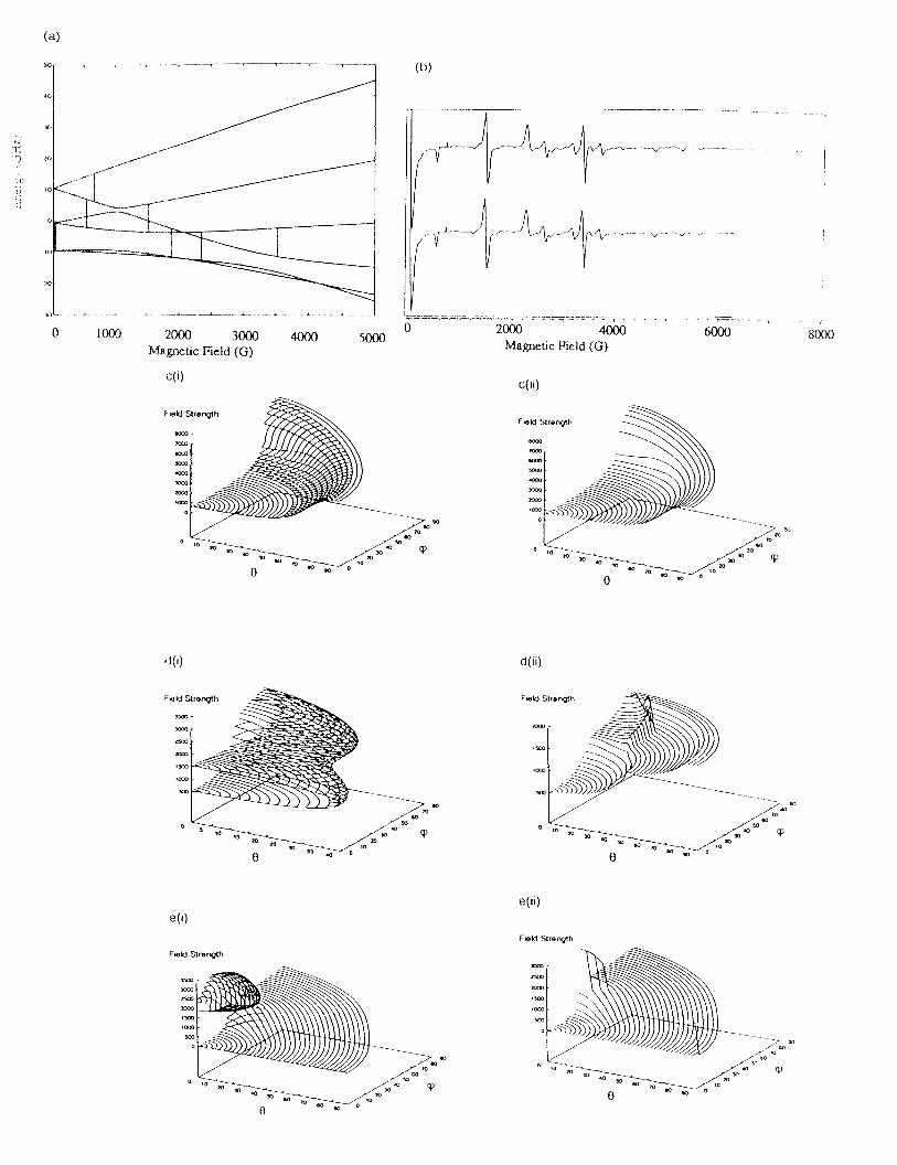
In the high spin Fe(III) example, if the microwave frequency ( Â = 9.0 GHz) is set slightly

smaller than the zero-field splitting, then multiple transitions can occur between a given pair of

energy levels. For example, three transitions at B = 3.525, 189.2 and 235.50 mT are observedres

between energy levels 2 and 4 (numbered in increasing energy), Figure 4a.

The power of homotopy in comparison to matrix diagonalization is clearly demonstrated in

Figure 4c-e which compares transition surfaces from the two methods for particular transitions

arising from an S=5/2 spin system. Figure 4c shows the transition surfaces between levels 5 and 6.

The homotopy surface (Figure 4c(i)) shows exactly the same structure as calculated by matrix

diagonalization (Figure 4c(ii)). This transition surface varies continuously as a function of the Euler

21

angles and the magnetic field B. Clearly, homotopy reproduces the surface obtained by matrix

diagonalization between levels 5 and 6 as the relative error [18] between the two methods is very

small 4.104334x10 . The transition surface from level 3 to level 5 shown in Figure 4d is an example-5

of a looping transition in which the transition surface folds back on itself. Whilst the surface is fully

defined by homotopy (Figure 4d(i)), the surface calculated by matrix diagonalization is incomplete

and erroneous since there no transitions between levels 3 and 5 when à > 40 (Figure 4d(ii)). InO

Figure 4e an anti-level crossing between levels 2 and 4 is graphed. Homotopy (Figure 4e(i)) resolves

the complete structure while matrix diagonalization completes only the mostly continuous lower

transition (Figure 4e(ii)). In this case matrix diagonalization may have found multiple points. Matrix

diagonalization may have discarded some points in completing the surface, as it is unable to make a

connection between the multivalued points. Note that the unmatched homotopy points indicate

structure not revealed with matrix diagonalization, while the points where matrix diagonalization and

homotopy do not agree indicate erroneous points calculated by matrix diagonalization. Randomly

orientated spectra calculated with homotopy and matrix diagonalization are shown in Figure 4b and

clearly there is excellent agreement between the two methods for this spin system.

The second example is a high spin (S=7/2) Gd(III) spin system for which the spin Hamiltonian

is given in Eq. [13]. The spin Hamilonian parameters are as follows: g = 1.9923, g = 1.9911, D =Ä Å1.8703 GHz, E/D = 0.19857, b =-0.0331, b =0.0288, b =0.0010, b =0.0011, b =0.0300,4 4 4 6 6

0 2 4 0 2

b =0.0309, b =0.0176 GHz and the microwave frequency was 9.4327 GHz. The transition surfaces6 64 6

(Figure 5a,b), calculated with Homotopy, for the transitions between energy levels 2-5 and 4-7 reveal

the presence of looping transitions. Interestingly, the randomly orientated spectra calculated with

matrix diagonalization (Figure 5a) and Homotopy (Figure 5b) are almost identical as revealed by the

difference spectrum (Figure 5c).

Æ Ç È a É bMI É cM 2I É dM 3

I

22

(14)

The comparison of a complexity analysis [18] reveals that Homotopy (~4/3 d N m ) will be3 2

more eff icient than matrix diagonalization (~ 1000 N m ) when the number of transitions (d) is less3 2

than seventy hundred and fifty. For the high spin Fe(III) and Gd(III) spin systems described above,

homotopy (Fe(III) , 149s; Gd(III) ,550s) was three and a half times faster than matrix diagonalization

(Fe(III) , 536s; Gd(III) , 1965s) on a Sili con Graphics R5000 O2 workstation with 256Mb of memory.

7. L inewidth Models

A number of linewidth models originally developed for magnetically isolated paramagnetic

species have been incorporated into the XSophe computer simulation software suite. For all the

linewidth models discussed below the linewidth parameter, Ê , is given in energy units. In SopheË(field space version), Ì is converted to a field-domain linewidth parameter Í through Í = |dB/dEË B B ij

| Ì (where B is the magnetic field and E = E - E ) [1, 22]. |dB/dE | is calculated for each transitionË ij i j ij

by using eigenfield perturbation theory [31]. This correction is not required with Homotopy when

the simulation is performed in frequency space (Section 8).

Although Sophe was primarily written for simulating randomly oriented EPR spectra, it can

also simulate solution (isotropic) EPR spectra. Incomplete averaging of the anisotropic g and A

matrices is dealt with using Kivelson's linewidth model [36]

The coeff icients a, b, c, and d can be related to the solvent viscosity, correlation time, molecular

hydrodynamics radius and the anisotropy of the spin system under study [36]. For systems with

couplings to multiple nuclei, the user can choose the nucleus on which the model is based.

The simplest anisotropic linewidth model is based on the angular variation of the g-values [1].

Î 2Ï Ð ( Î 2x g2

x l 2x Ñ Î 2

y g2y l 2

y Ñ Î 2z g2

z l 2z ) /g2

Î 2Ï Ð ( Òi Ó x,y,z

{ Ô 2Ri Õ [ Ö gi

gi × 0(B) Ø Ù Ai MI ]2} g2

i l 2i ) / g2

23

(15)

(16)

where g = g l + g l + g l , Ú 's (i=x,y,z) are the input linewidth parameters and l 's (i=x,y,z)2 2 2 2 2 2 2x x y y z z i i

are the direction cosines of the magnetic field with respect to the principal axes of the g matrix.

A more sophisticated approach is correlated g-A strain model which was originally developed

by Froncisz and Hyde [37] and has been used successfully to account for the linewidth variations

encountered in spin S=1/2 systems particularly in copper and low spin cobalt ( S=1/2 ) complexes

[1,3,37]. When expressed in the frequency-domain [1,22], the linewidth in this model is based on the

formulae

where the Ú (i =x, y, z) are the residual linewidths due to unresolved metal and/or ligand hyperfineRi

spli tting, homogeneous linewidth broadening, and other sources, Û g 's and Û A 's are the widths ofi i

the Gaussian distributions of the g and A values. The g-A strain model involves nine parameters for

a rhombically distorted metal ion site.

For S > ½ spin systems, the distribution of D and E values is likely to be the dominant factor

contributing to the linewidth. The distribution of D and E values arising from local strains at the

paramagnetic site results in a broadening of the spectral lines. Wenzel and Kim [38] have described a

statistical D-E strain model. In their model, the distributions of D and E are assumed to be

Gaussian and independent of each other, the resulting full width at maximum slope due to strain

alone is given by

Ü 2DE Ý Ü 2

D { < Þ i |S2z | Þ i > ß < à j |S

2z | à j>} 2á â 2

E{ < à i |S2x ß S2

y | à i > ß < à j |S2x ß S2

y | à j >} 2

ã 2ä å æ 2DE ç è 2

R

24

(17)

(18)

where é and é are the half-widths at maximum slope of the distributions of D and E in energy units,D E

respectively, and ê and ê are the wavefunctions associated with transition i ë j. This model wasi j

easily implemented in our program as full matrix diagonalisation employed in the program allows the

expectation values of the spin operators in Eq. [17] to be easily evaluated. In order to include other

sources of line broadening such as unresolved hyperfine interactions, a term representing the

residual linewidth, ì , is convoluted with the D-E strain effectsR

Here an assumption is made that the strain effects ( ì ) and other sources of line broadening ( ì )DE R

are statistically independent and they are all Gaussian distributions.

8. Computer Simulations in Frequency Space

In practice the EPR experiment is a field swept experiment in which the microwave frequency

( í ) is kept constant and the magnetic varied. Computer simulations performed in field space assumec

a symmetric lineshape function f in Eq. [1] (f(B-B ), î ) which must be multiplied by d í /dB and ares B

constant transition probabili ty across a given resonance.[1,22] In fact Pilbrow has described the

limitations of this approach in relation to asymmetric lineshapes observed in high spin Cr(III) spectra

and the presence of a distribution of g-values (or g-strain broadening). The following approach has

been employed by Pilbrow et al. in implementing Eq. [1] (frequency swept) into computer simulation

programmes based perturbation theory [1,9]. Firstly, at a given orientation of ( ï , ð ), the resonant

field positions (B ) are calculated with perturbation theory and then transformed into frequencyres

25

space ( ñ (B)). Secondly, the lineshape (f( ñ - ñ (B), ò ) and transition probabili ty are calculated in0 c 0 ófrequency space across a give resonance and the intensity at each frequency stored. Finally, the

frequency swept spectrum is transformed back into field space. Performing computer simulations in

frequency space produces assymmetric lineshapes (without having to artificially use an asymmetric

lineshape function) and secondly, in the presence of large distribution of g-values will correctly

reproduce the downfield shifts of resonant field positions.[9]

Unfortunately, the above approach cannot be used in conjunction with matrix diagonalization

as an increased number of matrix diagonalizations would be required to calculate f and the transition

probabili ty across a particular resonance. However, since Homotopy is in general three to five times

faster than matrix diagonalization we have adapted Homotopy to allow simulations to be performed

in frequency space. In order to determine how the microwave frequency varies with respect to the

magnetic field, the corresponding pair of eigenvalues are evaluated at a distribution of field strengths

across the lineshape. Also, since the transition probabili ty may not be constant over the lineshape, the

pair of eigenvectors and hence the probabili ty is also evaluated at each of these field strengths. A

cubic spline is then fit over these field strengths to accurately produce the lineshape.

An example which shows the difference between field and frequency space computer

simulations are shown in Figure 6. A single crystal EPR spectrum of the Cr(III) ( S=3/2, I=3/2) in

ruby calculated with matrix diagonalization in field space (Figure 6a) clearly shows symmetric

lineshapes, whilst the simulation performed in frequency with Homotopy (Figure 6b) reveals

asymmetric lineshapes arising from a variation in the transition probabili ty across the resonance.

Similar observations have been made by Pilbrow et al. who used perturbation based programmes

[1,22,39].

GF ô ( õ N

i ö 1

( Yexp ÷ S(B, ø c) ù ú )2)1/2 / ( N û ü )

26

(19)

9. Parallelisation

With the advent of multiprocessor computers and the new algorithms described above the

simulation of EPR spectra from complex spin systems consisting of multiple electron and or nuclear

spins becomes feasible with Sophe. Optimisation of the spin Hamiltonian parameters by the

computer will also be possible for these spin systems. Parallelisation of the matrix diagonalization

method has been performed at the level of the vertices in the Sophe grid. For example, if a computer

has 5 processors then the number of Sophe grid points is divided into groups of five and each group

is then processed by a one of the processors with the resultant spectra being added to an array shared

by the five processors. For the hypothetical Cr(III) spin system shown in Figure 3 a three-fold

reduction in computational time is observed. Greater reductions are observed for more complex spin

systems.

Parallelisation of homotopy, not yet implemented, is envisioned to occur at the transition

surface level, whereby the multiple surfaces are calculated simultaneously by multiple processors.

10. Optimisation Methods

A unique set of spin Hamiltonian parameters for an experimental EPR spectrum is obtained

through minimising the goodness of fit parameter (GF)

where the experimental spectrum (Y ) has been baseline corrected assuming a linear baseline andexp

the simulated spectrum has been scaled ( ú ) to Y . N is the number of points in common betweenexp

the experimental and simulated spectra and ü is the magnitude of noise in the spectrum. In the past

minimising GF has been performed through a process of trial-and-error by visually comparing the

27

simulated and experimental spectra until a close match was found. Recent progress in reducing

computational times for computer simulations (Sections 3-7) and the improved speed of

workstations allows the use of computer-based optimisation procedures to find the correct set of spin

Hamiltonian parameters from a given EPR spectrum.

The most appropriate technique for optimising a set of spin Hamiltonian parameters is

nonlinear least squares [40]. This method has the advantage that the differences (Y - S(B, ý ), Eq.exp c

14) associated with the more extreme positive or negative values are exaggerated, which emphasises

genuine peak mis-matching whilst tending to reduce the impact of noise. Unfortunately, evaluation

of S(B, ý ) can take a long time and as there is no analytic derivative information available, thisc

method is not really an option for general spin systems. Consequently, we have considered direct

search and Monte-Carlo methods.

Direct search methods are characterised by evaluating the function at several points within the

spin Hamiltonian parameter space ( þ -space) [41] and then using the knowledge gained during theP

last few evaluations in an attempt to choose a more promising point. These methods have lost

popularity over time, and have been largely superseded by methods using derivative information,

although they are still used in places where noise is prevalent. They suffer only two drawbacks: the

algorithms are particularly susceptible to becoming trapped in local minima; and they tend to be fairly

inefficient in their use of function evaluations (at least in comparison with derivative-based methods

on functions where derivatives are available). Three of these direct methods were considered

particularly promising, the Hooke and Jeeve's [42], Simplex [43] and a Quadratic method based on

the Hooke and Jeeves method.

28

The classic Monte-Carlo method is simply a random walk about the ÿ -space. Usually, stepsP

which lead to a function decrease are accepted, and those which do not are rejected (ie. another

point is chosen within a given radius of the current point). These methods are considerably more

wasteful of function evaluations than even the ad-hoc methods. However one of the Monte-Carlo

methods, simulated annealing, has the attraction of being a global optimisation strategy [44]. Global

minimisers are those which are not defeated by local minima, but rather given enough time find the

smallest minimum, or “global” minimum.

10.1 Hooke and Jeeve’s Method

The Hooke and Jeeve's method [42] was first publicised in 1961 and has been widely used for

some time. The method starts with an "exploratory" move. Each parameter is considered in turn, and

checks are made to see how changes made to the parameter affect the error. A fixed step is made in

the positive direction, and it is observed whether the error increases or decreases. If no improvement

is made, then a fixed step is made in the negative direction. Again it is observed whether the error is

improved. Based upon which fixed steps improved the error (but ignoring how much the error

changes), a direction for "pattern" moves is then determined. Fixed steps are then made along the

"pattern" direction until no further progress is made, at which stage another exploratory move is

made [41].

10.2 Quadratic Method

One of the problems observed while using the Hooke and Jeeve's method is that fixed steps are

made simply based on whether the error is increasing or decreasing, but ignoring how much each

parameter affects the error. During the "exploratory" move, three points are typically evaluated with

respect to each parameter. A quadratic can hence be drawn through these three points, and a

29

prediction can be made for the value of each parameter which minimises the error. Hence a quadratic

method was designed which is similar to the Hooke and Jeeve's method, but instead of using fixed

steps makes steps based upon a quadratic with respect to each parameter.

10.3 Simplex Method

The Spendley, Hext and Himsworth (or Simplex) method [43] has a very geometrical

interpretation. It works by taking an � + 1 vertex simplex (ie. a regular � + 1 sided figure inP P

� -space) and evaluating GF at each of the vertices. It then takes the vertex point with the largestP

value of GF (subject to a few restrictions) and replaces it with its reflection in the hyper-plane formed

by the other � points. P

The elegant nature of this algorithm is apparent in considering the case where � =2. TheP

problem can now be visualized by a three dimensional surface (ie. GF vs. the two � parameters)P

whose lowest point (valley/well) we aim to find. The simplex in this case is an equilateral triangle

which “rests” upon the three dimensional surface. The algorithm, simply dictates that the highest of

the three points will li ft over the other two, causing the triangle to “flip” over (so the highest point

now points down hill ). This process is repeated, and the triangle “flips” its way down to bottom of a

nearby minimum. If the triangle cannot flip to a new minimum, the size of the triangle is contracted

and termination takes place when the number of contractions reaches a defined limit.

The simplex method has two advantages over the Hooke and Jeeve's method. The first is its

use of � +1 evaluations of GF in determining the next point at which to evaluate S(B, � ) comparedP c

with the Hooke and Jeeve's method which uses at most two points (and then only during the pattern

step, it normally uses only one). The second advantage is that the simplex method is somewhat more

30

resili ent to local minima. This is because even if one of the points is very close to a local minimum,

then, if the simplex is still l arge enough, the simplex may well “flip out” of the well. Unfortunately, in

some circumstances, the simplex method can fail. To take a two-dimensional case, it is susceptible to

becoming trapped in a deep, narrow “valley” if one of the points lands very close to the bottom and

the other two points are different walls. Having reached this stage, no progress can be made except

along the valley (the sides are too steep to allow any climbing). If the point near the bottom is on the

down-hill side of the valley, then no movement can be made as the triangle cannot flip over a point,

only a line. Consequently, improvement is only possible with contractions occurring about the

lowest point which will result in early termination in a local minimum. A possible way to overcome

this diff iculty, is to combine the standard simplex algorithm described above with a stochastic process

(such as simulated annealing). This method would hopefully “break-out” of such minima. A brief

discussion of how this could be implemented is given after the description on simulated annealing.

10.4 Simulated Annealing

Simulated annealing is one of a class of methods known as Monte-Carlo methods[44]. The

simplest Monte-Carlo method starts at a point � and makes a random step of length l in � -spaceP P0

to the new point � . If GF ( � ) is less than � then the step is accepted and � is set to �P P P P P’ 0 ’ 0 0 1 ’ 0

at which point the process is repeated by taking a step from � . However if GF increases, then theP1

step is rejected and another step is taken from � . This process gradually forms a sequence of �P P0 s

with decreasing values of GF. The algorithm terminates with answer � when no more progress isPk

being made. At this point the algorithm may be restarted from this answer with a decreased step

size.

The concept of simulated annealing comes (somewhat loosely) from the annealing (solidifying)

31

of liquids (especially molten metals). The molecules in their liquid state have a high kinetic energy

which allows (indeed, forces) them to change their location and orientation. By cooling, their energy

is depleted and so they gradually “settle down” into what eventually becomes their fixed location.

The structure which results differs significantly depending upon the rate of cooling.

Simulated annealing attempts to emulate the slow cooling process by using one very significant

change from the standard Monte-Carlo method [44]. Rather than rejecting all function-increasing

steps, it accepts the “uphill ” kth step with probabili ty P( � , T), where P satisfies lim P=0. TheP k � �k

value T is known as the temperature of the system and decreases as k increases in accordance with a

cooling schedule. The hope is that the acceptance of a detrimental step will have long-term benefits

by allowing the sequence of � to “escape” from a local minimum. Ps

Two approaches for choosing a random point have been implemented into Sophe. In the first

method a random jump is performed by choosing a random point on a hypershere of radius r about

the current point. Both the temperature and the radius are decreased periodically throughout the

search. The benefit of this approach is that all � dimensions are searched simultaneously. In theP

second approach, each of the � axes are searched in turn. P

10.5 Parameter and Spectral Scaling

An important part of practical multi-variable optimisation is the sensitivity of scaling the

various spin Hamiltonian parameters. Since the Hooke and Jeeves and Simplex algorithms take finite

steps along various co-ordinate axes, there must be some uniformity in the rate of change in GF in

each of these directions. Since a change of � in one of the g values would have significantly less

effect on S(B, � ) than a step of � in one of the A values, then, without scaling, for any given stepc

32

size, only some of the variables will be usefully optimised. To solve this problem, the -spaceP

formed by the parameters to be varied is transformed to one where a given step length will have a

more uniform effect on GF in each of the directions. Given the necessity of avoiding costlyP

evaluations of S(B, ) and derivative information this can be done by performing a linearc

transformation by multiplying each of the spin Hamiltonian parameters by h. The h’s are manuallyi i

chosen to keep fluctuations in GF to approximately the same order of magnitude. Parameter scaling

is not required in the quadratic and simulated annealing approaches as the step size is dynamically

adjusted.

The simulated spectrum is multiplied by � (Eq. [14]) so that it can be directly compared to the

experimental spectrum, Y . In Sophe we have three methods for scaling, double integration (forexp

derivative EPR spectra), peak to peak extrema and optimisation of the scaling factor.

10.6 Spectral Comparison

Many complex randomly orientated EPR spectra contain overlapping resonances with complex

lineshapes. Optimisation of such spectra often leads to the computer broadening (increase in

linewidth) of one of the resonances to reduce the error. Although we do not profess to have the

ultimate solution to this problem, we have employed two approaches to help solve this problem. The

first approach involves the abili ty to control the sensitivity of parameter adjustment throughout the

optimisation procedure, whilst the second involves the comparison of the Fourier transformed

experimental and simulated spectra. The latter method provides increased resolution through

separating the high and low frequency components [45]. As an aid to optimising the computer

simulation XSophe/Xepr has the capabili ty of displaying intermediate spectra (Magnetic Field vs.

Intensity vs. Iteration Number) and the corresponding spin Hamiltonian parameters. An example of

33

such a display is shown in Figure 7 for the simulation of an isotropic spectrum arising from a Ag(II )

porphyrin like complex.

11. Concluding Remarks

Herein we have described a number of new developments (Sophe partition and interpolation

schemes, field segmentation, parallelisation and optimisation methods) which will provide scientists

with the tools for analysing randomly orientated, single crystal and isotropic EPR spectra. Inclusion

of Homotopy into the XSophe/Sophe EPR computer simulation suite has enabled:

� the tracing of a given transition as a function of orientation ( =0 � 180 , � =0 � 180) in theo o

presence of energy level anti-crossing,

� the tracing of looping transitions,

� computer simulations to be performed in frequency space and

� a reduction in the computational time.

When Homotopy is combined with the Sophe interpolation scheme we should obtain further

reductions in computational times without sacrificing accuracy. Homotopy may also be used in

conjunction with other partition schemes, for example the "Apple-peel" [1], "Igloo" [19], "Spiral"

[25], and "Triangular" [24] methods and perturbation theory.

Consequently, in conjunction with the Sophe partition scheme Homotopy improves the quality

of simulated spectra, allows the analysis of more complicated EPR spectra from complex spin

systems and reduces the computational time compared with matrix diagonalization. The method is

being currently extended to the simulation of field dependent CW-ENDOR, ESEEM, pulsed

ENDOR, solid state NMR and nuclear quadrupole resonance spectra.

34

12. Acknowledgements

The authors would like to thank the Australian Research Council and the EPR Division of

Bruker Analytik for financial support. MG and CE acknowledge the University of Queensland for the

provision of PhD and Bsc (Hons) scholarships respectively.

35

13. References

[1] J. R. Pilbrow, “Transition Ion Electron Paramagnetic Resonance”, Clarendon Press, Oxford,

(1990).

[2] F. E. Mabbs and D. C. Colli son, “Electron Paramagnetic Resonance of Transition Metal

Compounds” , Elsevier, Amsterdam, (1992).

[3] R. Basosi, W.E. Antholine, J.S. Hyde, “Multifrequency ESR of Copper Biophysical

Applications” in “Biological Magnetic Resonance” (L.J. Berliner, J. Reuben Eds.) Vol. 13,

New York, Plenum Press, (1993).

[4] G.R. Hanson, A.A. Brunette, A.C. McDonell, K.S. Murray, and A.G. Wedd, J. Amer. Chem.

Soc., 103, (1981) 1953.

[5] Y.S. Lebedev, Appl. Magn. Reson., 7, (1994) 339.

[6] L.C. Brunel, Appl. Magn. Reson., 11, (1996) 417.

[7] E.J. Reijerse, P.J. vanDam, A.A.K. Klaassen, W.R. Hagen, P.J.M. vanBentum, G.M. Smith,

Appl. Magn. Reson., 14, (1998) 153.

[8] Abragam, A., Bleaney, B.,: Electron Paramagnetic Resonance of Transition Ions. Clarendon

Press, Oxford (1970).

[9] A. Bencini and D. Gatteschi, “EPR of Exchange Coupled Systems”, Springer-Verlag, Berlin,

(1990).

[10] T. D. Smith and J. R. Pilbrow, Coord. Chem. Rev., 13, (1974) 173.

[11] P. C. Taylor, J. F. Baugher and H. M. Kriz, Chem. Rev., 75, (1975) 203.

[12] (a) J. D. Swalen and H. M. Gladney, IBM J. Res. Dev., 8, (1964) 515.

(b) J. D. Swalen, T. R. L. Lusebrink and D. Ziessow, Magn. Reson. Rev., 2, (1973) 165.

[13] H. L. Vancamp and A. H. Heiss, Magn. Reson. Rev., 7, (1981) 1.

[14] B.J. Gaffney, H.J. Silverstone, “Simulation of the EMR Spectra of the High-Spin iron in

36

proteins” in “Biological Magnetic Resonance”, (L.J. Berliner, J. Reuben Eds.) Vol. 13, New

York, Plenum Press, (1993).

[15] S. Brumby, J. Magn. Reson., 39, (1980) 1, ibid 40, (1980) 157.

[16] D. Wang, G.R. Hanson, J. Magn. Reson. A, 117, (1995) 1.

[17] D. Wang, G.R. Hanson, Appl. Magn. Reson., 11, (1996) 401.

[18] K.E. Gates, M. Griff in, G.R. Hanson, K. Burrage, J. Magn. Reson., 135, (1998) 104.

[19] (a) R. L. Belford and M. J. Nilges, EPR Symposium 21st Rocky Mountain Conference,

Denver, Colorado, (1979).

(b) A. M. Maurice. PhD thesis, University of Illi nois, Urbana, Illi nois, (1980).

(c ) M. J. Nilges, “Electron Paramagnetic Resonance Studies of Low Symmetry Nickel(I) and

Molybdenum(V) Complexes” , PhD thesis, University of Illi nois, Urbana, Illi nois, (1979).

[20] M. C. M. Gribnau, J. L. C. van Tits, E. J. Reijerse, J. Magn. Reson., 90, (1990) 474.

[21] A.Kretter, J. Huttermann, J. Magn. Reson. 93, (1991) 12.

[22] J. R. Pilbrow, J. Magn. Reson., 58, (1984) 186.

[23] E. Anderson, Z. Bai, C. Bischof, J. Demmel, J. Dongarra, J. Du Croz, A. Greenbaum, S.

Hammarling, A. McKenney, S. Ostrouchov, and D. Sorensen, “LAPACK Users' Guide”,

SIAM, Philadelphia, (1992).

[24] D. W. Alderman, M. S. Solum and D. M. Grant, J. Chem. Phys., 84, (1986) 3717.

[25] M. J. Mombourquette and J. A. Weil, “Simulation of Magnetic Resonance Powder Spectra. J.

Magn. Reson., 99, (1992) 37.

[26] G. van Veen, J. Magn. Reson., 38, (1978) 91.

[27] B.-Q. Su, D.-Y. Liu, “Computational geometry - Curves and Surface Modelli ng” , Academic

Press, Singapore, (1989).

[28] D. Nettar, N.I. Vill afranca, J. Magn. Reson., 64, (1985) 61.

37

[29] M.I. Scullane, L.K. White, N.D. Chasteen, J. Magn. Reson., 47, (1982) 383.

[30] D.G. McGavin, M.J. Mombourquette, J.A. Weil, “EPR ENDOR User’s manual” , University of

Saskatchewan, Saskatchewan, Canada, (1993).

[31] G.G. Belford, R.L. Belford, J.F. Burkhalter, J. Magn. Reson., 11, (1973) 251.

[32] T. Y. Li and N. H. Rhee, Numer. Math., 55, (1989) 265.

[33] M. Oettli, Technical Report 205, Department Informatik, ETH, Zürich, Dec. (1993). and

references therein.

[34] S. K. Misra, P. Vasilopoulos, J. Phys. C: Solid St. Phys., 13, (1980) 1083.

[35] G. H. Golub, C. F. Van Loan, Matrix Computations. Johns Hopkins University Press,

Baltimore, Maryland, (1983).

[36] (a) D. Kivelson, J. Chem. Phys. 33, (1960) 1094.

(b) R. Wilson, D. Kivelson, J. Chem. Phys. 44, (1966) 154, ibid 44, (1966) 4440.

(c) P.W. Atkins, D. Kivelson, J. Chem. Phys. 44, (1966) 169.

[37] (a) W. Froncisz, J.S. Hyde, J. Chem. Phys. 73, (1980) 3123.

(b) J.S. Hyde, W. Froncisz, Ann. Rev. Biophys. Bioeng. 11, (1982) 391.

[38] R.F. Wenzel, Y.W. Kim, Phys. Rev. 140, (1965) 1592.

[39] (a) G. R. Sinclair, “Modelli ng Strain Broadened EPR Spectra”, PhD thesis, Monash University,

(1988).

(b) J.R. Pilbrow, G.R. Sinclair, D.R. Hutton, G.J. Troup, J. Mag. Reson., 52, (1983) 386.

[40] (a) S.K. Misra, J. Mag. Reson., 23, (1976) 403.

(b) S.K., Misra, Mag. Reson. Rev., 10, (1986) 285.

(c) S.K., Misra, Physica, 121B, (1983) 193.

(d) S.K., Misra, S. Subramanian, J. Physics C, 15, (1982) 7199.

[41] Spin Hamiltonian parameters are constrained to a portion of � -space as this will prevent theP

38

generation of a NULL spectrum.

[42] R. Hooke, T.A. Jeeves, J. Assoc. Computing Machinery, 8, (1961) 212.

[43] W. Spendley, G.R. Hext, F.R. Himsworth, Technometrics, 4, (1962) 441.

[44] (a) D.M. Nicholson, A. Chowdhary, L. Schwartz, Physical Review B, 29, (1984) 1633.

(b) I.O. Bohachevsky, M.E. Johnson, L.S. Myron, Technometrics, 28, (1986) 209.

(c) A. Corana, M. Marchesi, C. Martini, S. Ridella, ACM Trans. Math. Software, 13, (1987)

262.

(d) H. Heynderickx, H. De Raedt, D. Schoemaker, J. Magn. Reson., 70, (1986) 134.

[45] R. Basosi, G. Della Lunga, R. Pogni, Appl. Magn. Reson., 11, (1996) 437.

39

List of Figures

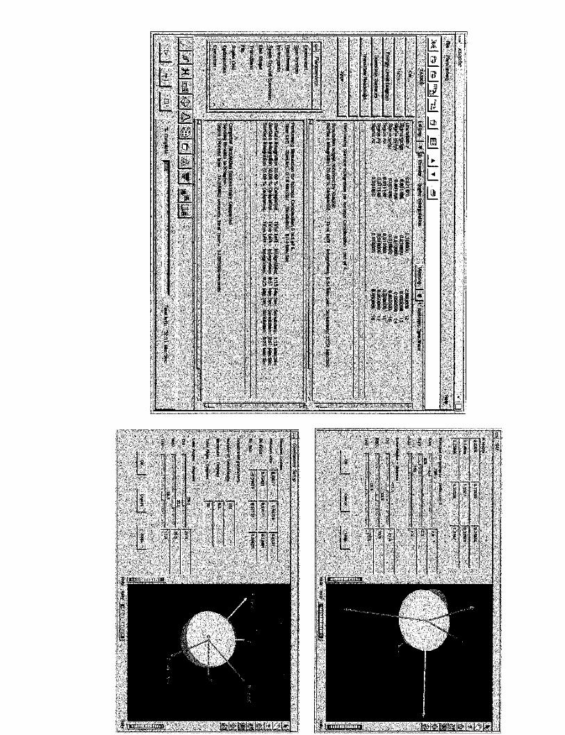
Figure 1. The XSophe interface allows the creation and execution of multiple input files on the

local or remote hosts. There are macro task buttons to guide the novice through the

various menus and two button bars to allow easy access to the menus. For example the

bottom bar (left to right), Experimental Parameters, Spin System, Spin Hamiltonian,

Instrumental Parameters, Single Crystal Settings, Lineshape Parameters, Transition

Labels/Probabili ties, File Parameters, Sophe Grid Parameters, Optimisation Parameters,

Execution Parameters and Batch Parameters. (a) Main window, (b) Anisotropic

hyperfine parameter dialog, (c) Single crystal parameter dialog.

Figure 2. A schematic representation of the SOPHE partition scheme. (a) Vertex points with a

SOPHE partition number N = 10; (b) the SOPHE partition grid in which the three sets of

curves are described by Eq. [4]. (c) Subpartitioning into smaller triangles can be

performed by using either Eq. [4] or alternatively the points along the edge of the triangle

are interpolated by the cubic spline interpolation method [24] and each point inside the

triangle is linearly interpolated three times and an average is taken.

Figure 3. Computer simulations of the powder EPR spectrum from a fictitious spin system (S=3/2;

I=3/2) which demonstrates the efficiency of the SOPHE interpolation scheme. (a)

Without the SOPHE interpolation scheme, N=18, (b) With the SOPHE interpolation

scheme, N=18 and (c) Without the SOPHE interpolation scheme, N=400. The

computational times were obtained on a SGI O2 R5K (180 MHz). � =34 GHz; field axis

resolution: 4096 points; an isotropic Gaussian lineshape with a half width at half

maximum of 30 MHz was used in the simulation.

Figure 4 A comparison of Homotopy and matrix diagonalization methods for the computer

simulation of a randomly orientated EPR spectrum for a high spin Fe(III) complex with

40

D=0.1 cm , E/D=0.25, g=2.0, � =9.0 GHz. (a) Energy level diagram, (b) Randomly-1

orientated spectra calculated with (i) homotopy and (ii) matrix diagonalization, (c)

Transition surfaces as a function of � , � and B for transitions between levels 5 and 6, (i)

homotopy, (ii) matrix diagonalization, (d) as for (c) except the surfaces relate to the

thransition between levels 3 and 5, (e) as for (c) except the surfaces relate to the

thransition between levels 2 and 4.

Figure 5 Computer simulation of a Gd(III) EPR spectrum (g = 1.9923, g = 1.9911, D = 1.8703� �

GHz, E/D = 0.19857, b =-0.0331, b =0.0288, b =0.0010, b =0.0011, b =0.0300,4 4 4 6 60 2 4 0 2

b =0.0309, b =0.0176 GHz and � =9.4327 GHz). with Homotopy. (a) Transition6 64 6

surfaces between levels between energy levels 2 and 5, (b) Transition surfaces between

levels between energy levels 4 and 7, (c) Randomly orientated EPR spectra calculated

with matrix diagonalization (top), Homotopy (middle) and the difference spectrum

(bottom).

Figure 6 Computer simulated EPR spectrum from a single crystal of ruby. (a) Frequency swept

simulation employing Homotopy, (b) Field swept simulation employing matrix

diagonalization, (c) Difference spectrum.

Figure 7 Spectral optimisation using the Hooke and Jeeve’s method for optimising the spin

Hamiltonian parameters for a Ag(II) porphyrin like complex. g = 2.05986, A( Ag) =iso107

32.83, A( N) = 20.95 10 cm . The two dimensional (Magnetic field vs. Iteration14 -4 -1

number) plot reveals the progress in minimising GF.

44

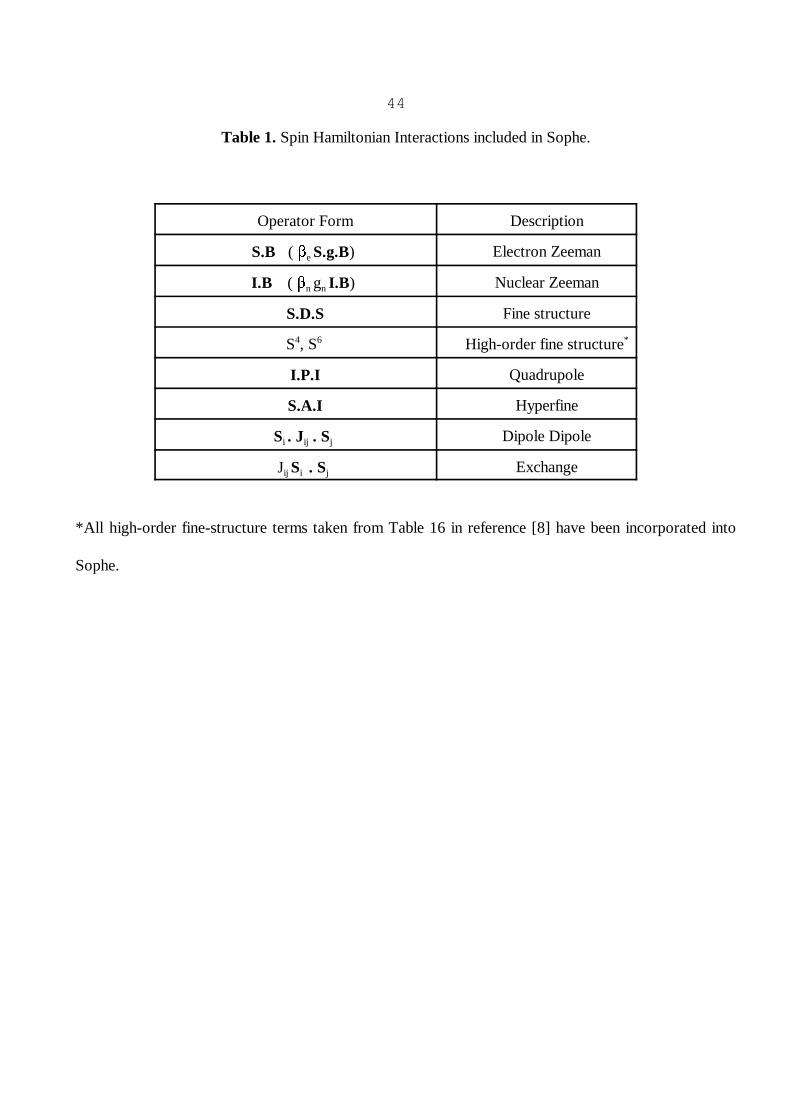
Table 1. Spin Hamiltonian Interactions included in Sophe.

Operator Form Description

S.B ( � S.g.B) e Electron Zeeman

I .B ( � g I .B) n n Nuclear Zeeman

S.D.S Fine structure

S , S High-order fine structure4 6 *

I .P.I Quadrupole

S.A.I Hyperfine

S . J . S i ij j Dipole Dipole

J S . S ij i j Exchange

*All high-order fine-structure terms taken from Table 16 in reference [8] have been incorporated into

Sophe.