Xplor-NIH: An Introduction

Charles SchwietersCenter for Information Technology

National Institutes of Health

Bethesda, MD USA

Charles@Schwieters.org

January 13, 2016

1

outline1. description, history, installation

2. Scripting Languages: XPLOR, Python, TCL

• Introduction to Python

3. Overview of an Xplor-NIH Python script

4. Potential terms available from Python

5. IVM: dynamics and minimization in internal coordinates

6. Parallel determination of multiple structures

7. Water Refinement

8. VMD molecular graphics interface

9. Refinement against solution scattering data.

10. Ensemble refinement for a dynamical representation.

11. The PASD facility for automatic NOE assignment

goal of this session:

Overview of NMR structure determination. Xplor-NIH’s Python interface will be

introduced, described in enough detail such that scripts can be understood, and modified.

2

Major Contributors at NIHGuillermo Bermejo John Kuszewski

Yaroslav Ryabov Robin Thottungal

Marius Clore Nico Tjandra

Support:

Andy Byrd, Yun-Xing Wang, Ad Bax

developed in the Imaging Sciences Laboratory, DCB, CIT, NIH

Many contributions from the community

3

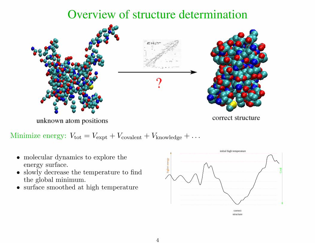
Overview of structure determination

Minimize energy: Vtot = Vexpt + Vcovalent + Vknowledge + . . .

• molecular dynamics to explore theenergy surface.

• slowly decrease the temperature to findthe global minimum.

• surface smoothed at high temperature

correctstructure

high

er e

nerg

y

initial high temperature

Coo

l

4

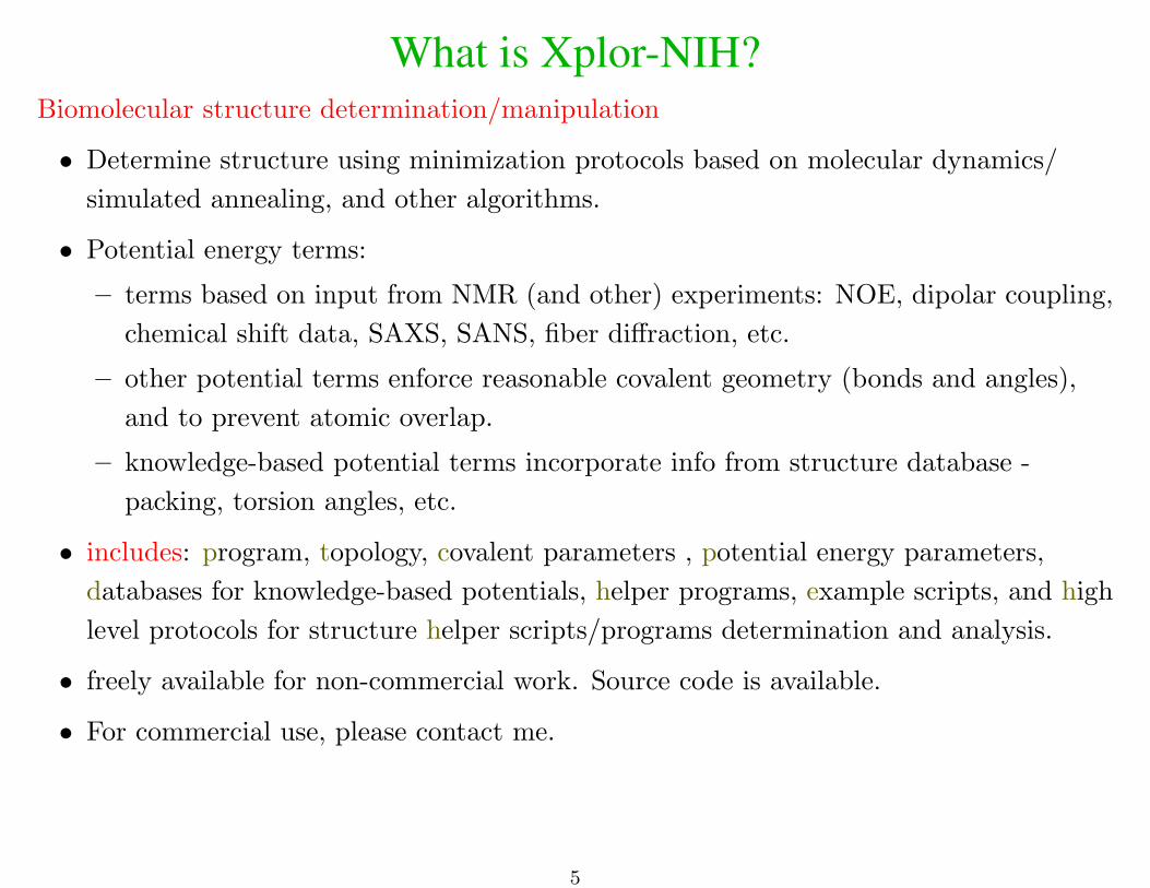
What is Xplor-NIH?Biomolecular structure determination/manipulation

• Determine structure using minimization protocols based on molecular dynamics/

simulated annealing, and other algorithms.

• Potential energy terms:

– terms based on input from NMR (and other) experiments: NOE, dipolar coupling,

chemical shift data, SAXS, SANS, fiber diffraction, etc.

– other potential terms enforce reasonable covalent geometry (bonds and angles),

and to prevent atomic overlap.

– knowledge-based potential terms incorporate info from structure database -

packing, torsion angles, etc.

• includes: program, topology, covalent parameters , potential energy parameters,

databases for knowledge-based potentials, helper programs, example scripts, and high

level protocols for structure helper scripts/programs determination and analysis.

• freely available for non-commercial work. Source code is available.

• For commercial use, please contact me.

5

Xplor-NIH Description

New contributions, additions are encouraged.

Source code of Xplor-NIH:

• original XPLOR Fortran source, with contributions from many groups.

• current work uses C++ for compute-intensive work.

• scripts and much code are written in Python, TCL scripting languages.

• SWIG used to “glue” scripting languages to C++.

• bazaar (bzr) repository of source code is available online.

6

XPLOR History1. approx. 1984. Initially a fork of CHARMM by Axel Brunger – for NMR and X-ray

structure determination.

2. rights sold to what is now Accelrys corp.

3. 1998. A. Brunger and coworkers develop replacement program CNS.

4. approx 2000. Xplor-NIH started.

5. 2002. Agreement between Accelrys and NIH allowing distribution of legacy XPLOR

code with Xplor-NIH. This allows complete backward compatibility with legacy

XPLOR scripts. C++, Python and TCL code has no restrictions.

6. approx 2007. Accelrys agreement expired, but no one cared. Accelrys will not

respond to NIH queries regarding Xplor-NIH. This complicates commercial use.

7. 2015. Issues with commercial distribution are being overcome.

7

Installation1. download two files from http://nmr.cit.nih.gov/xplor-nih/ (visit)

a) a -db file: e.g. xplor-nih-2.41.1-db.tar.gz

b) a platform-specific file: e.g. xplor-nih-2.41.1-Linux_x86_64.tar.gz

2. unpack these files where you wish them to live:

zcat xplor-nih-2.41.1-db.tar.gz | (cd /opt ; tar xf -)

zcat xplor-nih-2.41.1-Linux_x86_64.tar.gz | (cd /opt ; tar xf -)

3. perform initial configuration:

cd /opt/xplor-nih-2.41.1

./configure -symlinks /usr/local/bin

The optional -symlinks argument creates symbolic links in the specified directory for

xplor and other commands. It is intended that you specify a directory in your PATH.

For instance, if installing in your home directory, you might specify

-symlinks ~/bin.

4. test the new installation:

bin/testDist

8

Scripting Languages- three choicesscripting language:

• flexible interpreted language

• used to input filenames, parameters, protocols

• flexible enough to program non compute-intensive logic

• relatively user-friendly

XPLOR language:

strong point:

atom selection language quite powerful.

weaknesses:

String, Math support problematic.

no support for subroutines: difficult to encapsulate functionality.

Parser is hand-coded in Fortran: difficult to update.

XPLOR reference manual:

http://nmr.cit.nih.gov/xplor-nih/doc/current/xplor/

NOTE: all old XPLOR 3.851 scripts should run unmodified with Xplor-NIH.

9

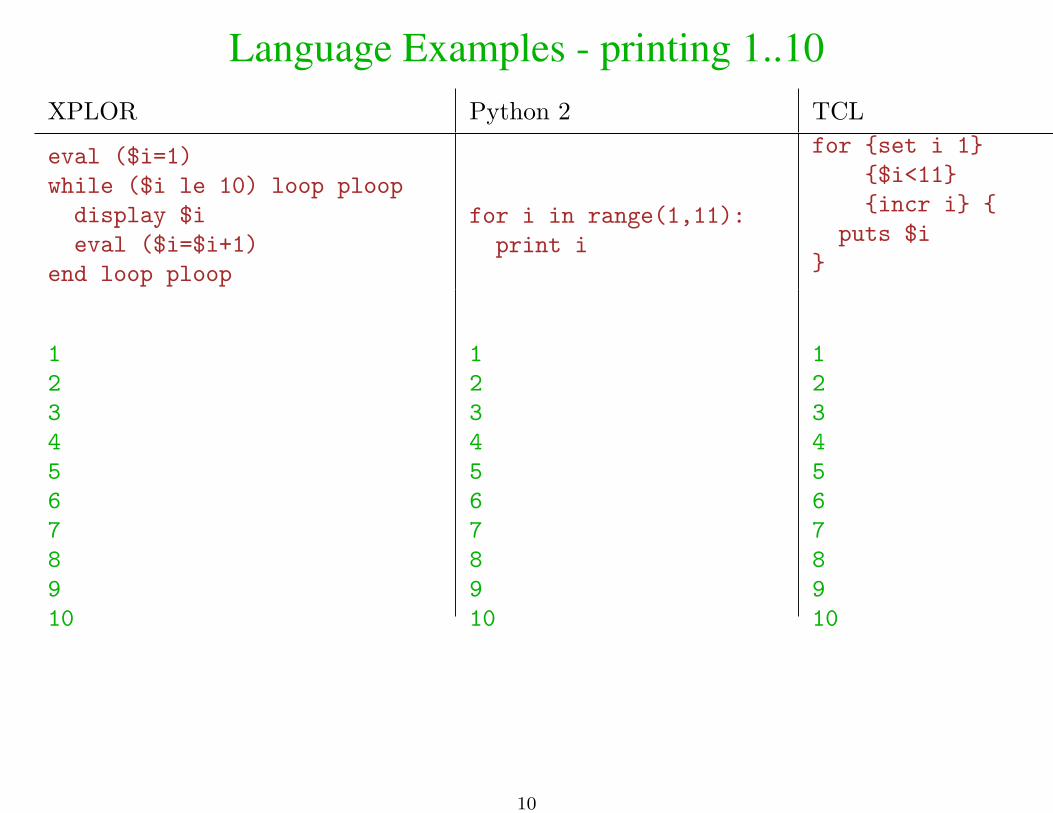
Language Examples - printing 1..10XPLOR Python 2 TCL

eval ($i=1)

while ($i le 10) loop ploop

display $i

eval ($i=$i+1)

end loop ploop

for i in range(1,11):

print i

for set i 1

$i<11

incr i

puts $i

1

2

3

4

5

6

7

8

9

10

1

2

3

4

5

6

7

8

9

10

1

2

3

4

5

6

7

8

9

10

10

General purpose scripting languages: Python and TCL• excellent string support.

• languages have functions and modules: can be used to better encapsulate protocols (

e.g. call a function to perform simulated annealing. )

• well known: these languages are useful for other computing needs: replacements for

AWK, shell scripting, etc.

• contain extensive libraries with additional functionality (e.g. file processing, web

access, GUI library, etc).

• Facilitate interaction, tighter coupling with other tools.

– NMRWish has a TCL interface.

– pyMol has a Python interface.

– VMD has TCL and Python interfaces.

– Allow tight integration with CING structure validation suite (currently being

implemented).

separate processing of input files (assignment tables) is unnecessary: can all be done

using Xplor-NIH.

11

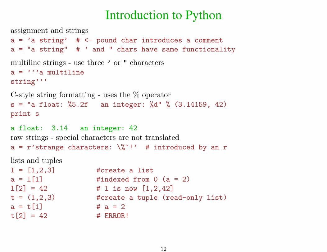
Introduction to Pythonassignment and stringsa = ’a string’ # <- pound char introduces a comment

a = "a string" # ’ and " chars have same functionality

multiline strings - use three ’ or " charactersa = ’’’a multiline

string’’’

C-style string formatting - uses the % operators = "a float: %5.2f an integer: %d" % (3.14159, 42)

print s

a float: 3.14 an integer: 42

raw strings - special characters are not translateda = r’strange characters: \%~!’ # introduced by an r

lists and tuplesl = [1,2,3] #create a list

a = l[1] #indexed from 0 (a = 2)

l[2] = 42 # l is now [1,2,42]

t = (1,2,3) #create a tuple (read-only list)

a = t[1] # a = 2

t[2] = 42 # ERROR!

12

Introduction to Pythoncalling functionsbigger = max(4,5) # max is a built-in function

defining functions - leading whitespace scopingdef sum(item1,item2,item3=0):

"return the sum of the arguments" # comment string

retVal = item1+item2+item3 # note indentation

return retVal

print sum(42,1) #un-indented line: not in function

43

using keyword arguments - specify arguments using the argument nameprint sum(item3=2,item1=37,item2=3) # argument order is not important

42

loops - the for statementfor cnt in range(0,3): # loop over the list [0,1,2]

cnt += 10

print cnt

10

11

12

13

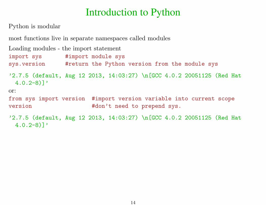
Introduction to PythonPython is modular

most functions live in separate namespaces called modules

Loading modules - the import statementimport sys #import module sys

sys.version #return the Python version from the module sys

’2.7.5 (default, Aug 12 2013, 14:03:27) \n[GCC 4.0.2 20051125 (Red Hat

4.0.2-8)]’

or:from sys import version #import version variable into current scope

version #don’t need to prepend sys.

’2.7.5 (default, Aug 12 2013, 14:03:27) \n[GCC 4.0.2 20051125 (Red Hat

4.0.2-8)]’

14

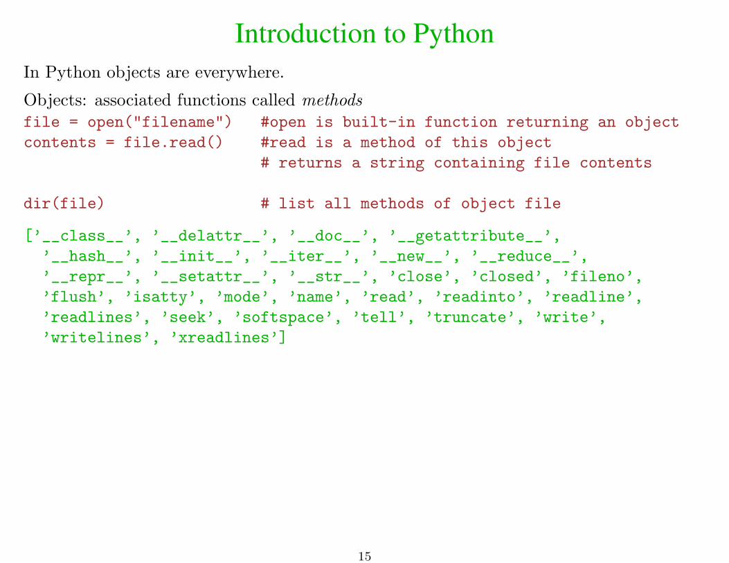
Introduction to PythonIn Python objects are everywhere.

Objects: associated functions called methodsfile = open("filename") #open is built-in function returning an object

contents = file.read() #read is a method of this object

# returns a string containing file contents

dir(file) # list all methods of object file

[’__class__’, ’__delattr__’, ’__doc__’, ’__getattribute__’,

’__hash__’, ’__init__’, ’__iter__’, ’__new__’, ’__reduce__’,

’__repr__’, ’__setattr__’, ’__str__’, ’close’, ’closed’, ’fileno’,

’flush’, ’isatty’, ’mode’, ’name’, ’read’, ’readinto’, ’readline’,

’readlines’, ’seek’, ’softspace’, ’tell’, ’truncate’, ’write’,

’writelines’, ’xreadlines’]

15

Introduction to PythonA mapping type: Dictionariesd=

d[’any’] = 4 #elements indexed like arrays

d[’string’] = 5 # but the index can be (almost) any type

print d[’string’]

5

d.keys() #return list of all index keys

d.values() #return list of all indexed values

Tools for List Processing:

List Comprehensions - convert a list to another liststringList=[’1’,’2’,’3’]

[ int(i) for i in stringList ] # convert list of string to ints

[1, 2, 3]

List comprehension:

• expression within square brackets containing for, in and optionally if

[ 2*int(c) for c in [’3’,’2’,’1’] if c!=’2’ ]

[6, 2]

16

Introduction to Pythoninteractive help functionality: dir() is your friend!import sys

dir(sys) #lists names in module sys

dir() # list names in current (global) namespace

dir(1) # list of methods of an integer object

the help functionimport ivm

help( ivm ) #help on the ivm module

help(open) # help about the built-in function open

help(sys.exit) # help about the exit function in the imported sys module

browse the Xplor-NIH python library using your web-browser on your local workstation:

% xplor -py -pydoc -g

Xplor-NIH Python module reference:

http://nmr.cit.nih.gov/xplor-nih/doc/current/python/ref/index.html

17

Linear Algebra Facilities in PythonDirect access to efficient C++ routines for matrix/vector manipulation. Includes

Numerical Python-like operations.

from cdsMatrix import RMat, transpose, inverse

from cdsMatrix import svd, trace, det, eigen

m=RMat([[1,2], #create a matrix object

[3,4]])

print m

print m[0,1] #element access

m[0,1]=3.14 #element assignment

print trace(m) #matrix trace

print det(m) #determinant

print transpose(m)#matrix transpose

print inverse(m) #matrix inverse

print 0.5*m # multiplication by scalar

print m+m,m-m # matrix addition, subtraction

print m*m # matrix multiplication

from cdsVector import CDSVector_double as vector

from cdsVector import norm

v=vector([1,2]) # vectors

print norm(v) # vector norm

print 2*v,v+v,v-v # vector arithmetic

print m*v # matrix multiplication

# 3-dimensional vectors

from vec3 import Vec3, cross, dot, unitVec

v = Vec3(1,2,3)

cross(Vec3(1,0,0),v) ; dot(Vec3(1,0,0),v)

unitVec(v)

# singular value decomposition

r= svd(m)

print r.u, r.vT, r.sigma

# eigenvalue decomposition

e= eigen(m)

print e[0].value() #first eigenvalue

print list(e[0].vector()) #first eigenvector

18

Additional Mathematical FacilitiesThese modules are distributed with Xplor-NIH.

• cminpack: nonlinear least squares.

• fft: real and complex FFTs.

• moremath: special functions and constants.

• spline: 1-, 2-, and 3- dimensional cubic splines.

• numpy: Numeric Python library is distributed with Xplor-NIH.

• matplotlib: powerful plotting package.

19

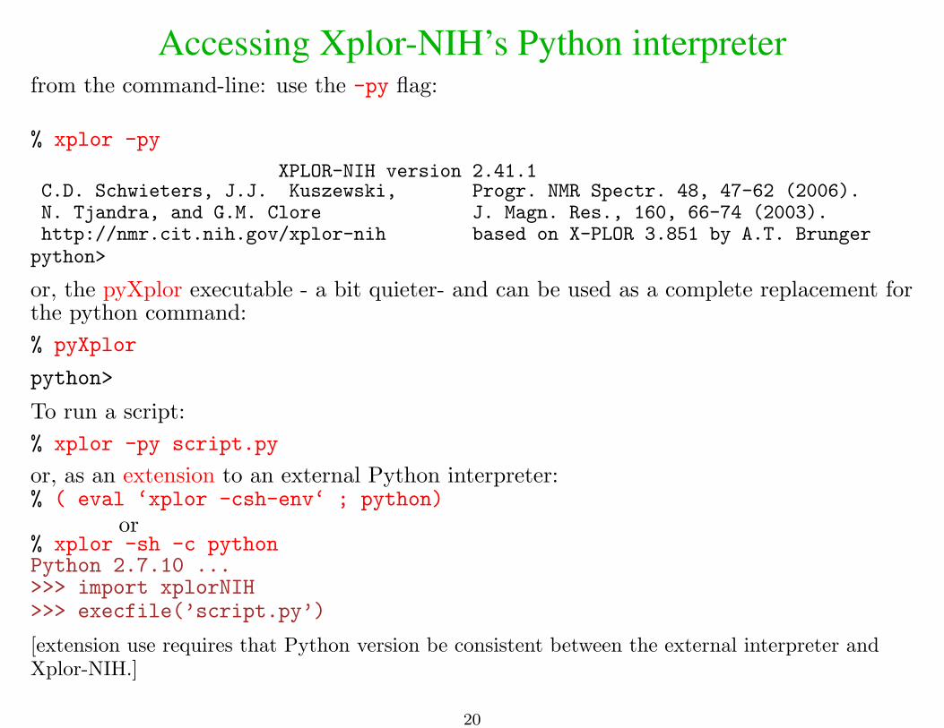
Accessing Xplor-NIH’s Python interpreterfrom the command-line: use the -py flag:

% xplor -py

XPLOR-NIH version 2.41.1C.D. Schwieters, J.J. Kuszewski, Progr. NMR Spectr. 48, 47-62 (2006).N. Tjandra, and G.M. Clore J. Magn. Res., 160, 66-74 (2003).http://nmr.cit.nih.gov/xplor-nih based on X-PLOR 3.851 by A.T. Brungerpython>

or, the pyXplor executable - a bit quieter- and can be used as a complete replacement forthe python command:

% pyXplor

python>

To run a script:

% xplor -py script.py

or, as an extension to an external Python interpreter:% ( eval ‘xplor -csh-env‘ ; python)

or% xplor -sh -c pythonPython 2.7.10 ...>>> import xplorNIH>>> execfile(’script.py’)

[extension use requires that Python version be consistent between the external interpreter andXplor-NIH.]

20

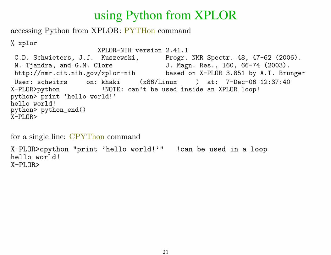
using Python from XPLORaccessing Python from XPLOR: PYTHon command

% xplorXPLOR-NIH version 2.41.1

C.D. Schwieters, J.J. Kuszewski, Progr. NMR Spectr. 48, 47-62 (2006).N. Tjandra, and G.M. Clore J. Magn. Res., 160, 66-74 (2003).http://nmr.cit.nih.gov/xplor-nih based on X-PLOR 3.851 by A.T. Brunger

User: schwitrs on: khaki (x86/Linux ) at: 7-Dec-06 12:37:40X-PLOR>python !NOTE: can’t be used inside an XPLOR loop!python> print ’hello world!’hello world!python> python_end()X-PLOR>

for a single line: CPYThon command

X-PLOR>cpython "print ’hello world!’" !can be used in a loophello world!X-PLOR>

21

using XPLOR, TCL from Pythonto call the XPLOR interpreter from Pythonxplor.command(’’’struct @1gb1.psf end

coor @1gb1.pdb’’’)

xplor is a built-in module - no need to import it for simple scripts.

to call the TCL interpreter from Pythonfrom tclInterp import TCLInterp #import functiontcl = TCLInterp() #create TCLInterp objecttcl.command(’xplorSim setRandomSeed 778’) #initialize random seed

22

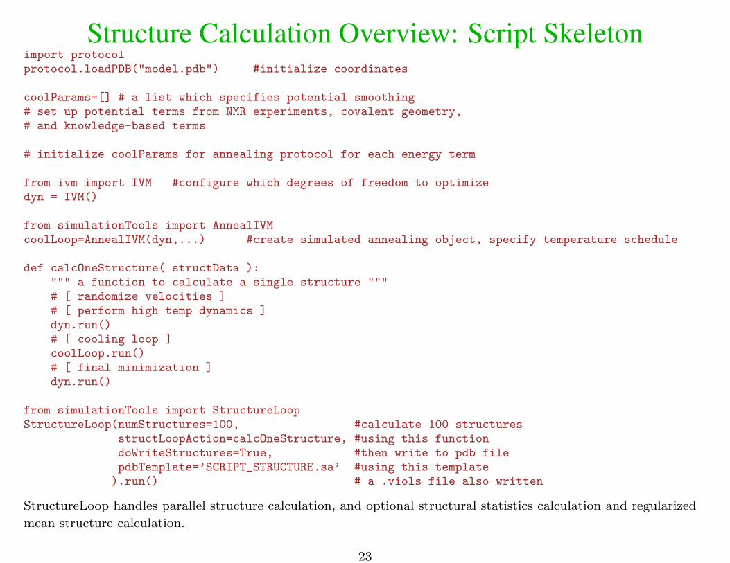
Structure Calculation Overview: Script Skeletonimport protocolprotocol.loadPDB("model.pdb") #initialize coordinates

coolParams=[] # a list which specifies potential smoothing# set up potential terms from NMR experiments, covalent geometry,# and knowledge-based terms

# initialize coolParams for annealing protocol for each energy term

from ivm import IVM #configure which degrees of freedom to optimizedyn = IVM()

from simulationTools import AnnealIVMcoolLoop=AnnealIVM(dyn,...) #create simulated annealing object, specify temperature schedule

def calcOneStructure( structData ):""" a function to calculate a single structure """# [ randomize velocities ]# [ perform high temp dynamics ]dyn.run()# [ cooling loop ]coolLoop.run()# [ final minimization ]dyn.run()

from simulationTools import StructureLoopStructureLoop(numStructures=100, #calculate 100 structures

structLoopAction=calcOneStructure, #using this functiondoWriteStructures=True, #then write to pdb filepdbTemplate=’SCRIPT_STRUCTURE.sa’ #using this template

).run() # a .viols file also written

StructureLoop handles parallel structure calculation, and optional structural statistics calculation and regularized

mean structure calculation.

23

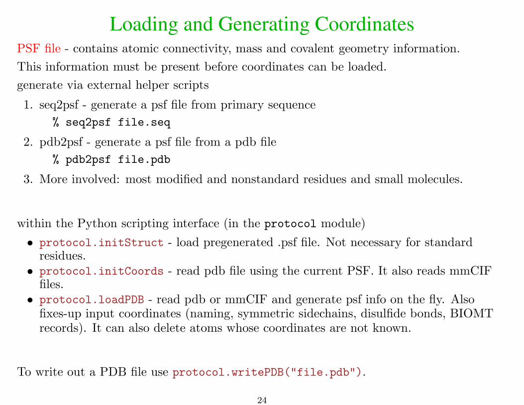
Loading and Generating CoordinatesPSF file - contains atomic connectivity, mass and covalent geometry information.

This information must be present before coordinates can be loaded.

generate via external helper scripts

1. seq2psf - generate a psf file from primary sequence

% seq2psf file.seq

2. pdb2psf - generate a psf file from a pdb file

% pdb2psf file.pdb

3. More involved: most modified and nonstandard residues and small molecules.

within the Python scripting interface (in the protocol module)

• protocol.initStruct - load pregenerated .psf file. Not necessary for standardresidues.• protocol.initCoords - read pdb file using the current PSF. It also reads mmCIF

files.• protocol.loadPDB - read pdb or mmCIF and generate psf info on the fly. Also

fixes-up input coordinates (naming, symmetric sidechains, disulfide bonds, BIOMTrecords). It can also delete atoms whose coordinates are not known.

To write out a PDB file use protocol.writePDB("file.pdb").

24

Loading and Generating Coordinates - detailsA Simulation object contains atom name, position, mass, etc and bonding information.

The default Simulation is xplor.simulation

A completely separate PSF can be loaded by creating a new XplorSimulation:from xplorSimulation import XplorSimulationnew_xsim = XplorSimulation()import protocolprotocol.initStruct(’other.psf’,simulation=new_xsim)

Each XplorSimulation has a separate XPLOR process associated with it.

Initial atomic coordinate values: (x,y,z) = (9999.999, 9999.999, 9999.999) theseare the values if coordinates are not initialized.

To delete these atoms:xplor.simulation.deleteAtoms("not known")

To add atomic coordinates if some are not defined:from protocol import addUnknownAtomsaddUnknownAtoms()

These coordinates will have proper covalent geometry.

To correct covalent geometry (bonds, angles and impropers):from protocol import fixupCovalentGeomfixupCovalentGeom(’resid 30:50’) # this may cause significant changes in

# the selected atomic positions

25

Topology and Parameters

Topology specifies how residues and (small)

molecules are connected.

Parameters specify force constants, bond lengths,

atomic radii, etc.

For standard proteins and nucleic acids, no special

action required.

For modified or artificial residues or small molecule

ligands, may need to generate new topology and

parameters:

• PRODRG http://davapc1.bioch.dundee.ac.

uk/cgi-bin/prodrg

• ACPYPE

http://webapps.ccpn.ac.uk/acpype/

Topology Entry for Alanineresidue ALA

group

atom N type=NH1 charge=-0.36 end

atom HN type=H charge= 0.26 end

group

atom CA type=CT charge= 0.00 end

atom HA type=HA charge= 0.10 end

group

atom CB type=CT charge=-0.30 end

atom HB1 type=HA charge= 0.10 end

atom HB2 type=HA charge= 0.10 end

atom HB3 type=HA charge= 0.10 end

group

atom C type=C charge= 0.48 end

atom O type=O charge=-0.48 end

bond N HN

bond N CA bond CA HA

bond CA CB bond CB HB1 bond CB HB2 bond CB HB3

bond CA C

bond C O

improper HA N C CB !stereo CA

improper HB1 HB2 CA HB3 !stereo CB

end

For water refinement (see Water Refinement below), alternate topology and parametersare required. Please see the examples.

26

Atom Selections in PythonWe use a subset of the XPLOR atom selection language, described here.from atomSel import AtomSelsel = AtomSel(’’’resid 22:30 and

(name CA or name C or name N)’’’)print sel.string() #AtomSel objs remember their selection string

resid 22:30 and(name CA or name C or name N)

AtomSel objects can be used as lists of Atom objectsprint len(sel) # prints number of atoms in selfor atom in sel: # iterate through atoms in sel

print atom.string(), atom.pos() # prints atom string, and its position.

AtomSel objects can be reevaluated:xplor.simulation.deleteAtoms("resid 1:2")sel.reevaluate()print len(sel) # prints the correct number of atoms

Atomwise AtomSel operations:from atomSel import intersection, union, notSelectionsel2 = AtomSel(’name C’)intersection(sel,sel2); union (sel,sel2); notSelection(sel)

Named atom selections:import atomSelLangatomSelLang.setNamedSelection(xplor.simulation,"nTerminus",

AtomSel("resid 1:140").indices())atoms = AtomSel(’recall nTerminus’)

27

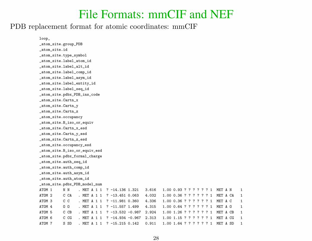
File Formats: mmCIF and NEFPDB replacement format for atomic coordinates: mmCIF

loop_

_atom_site.group_PDB

_atom_site.id

_atom_site.type_symbol

_atom_site.label_atom_id

_atom_site.label_alt_id

_atom_site.label_comp_id

_atom_site.label_asym_id

_atom_site.label_entity_id

_atom_site.label_seq_id

_atom_site.pdbx_PDB_ins_code

_atom_site.Cartn_x

_atom_site.Cartn_y

_atom_site.Cartn_z

_atom_site.occupancy

_atom_site.B_iso_or_equiv

_atom_site.Cartn_x_esd

_atom_site.Cartn_y_esd

_atom_site.Cartn_z_esd

_atom_site.occupancy_esd

_atom_site.B_iso_or_equiv_esd

_atom_site.pdbx_formal_charge

_atom_site.auth_seq_id

_atom_site.auth_comp_id

_atom_site.auth_asym_id

_atom_site.auth_atom_id

_atom_site.pdbx_PDB_model_num

ATOM 1 N N . MET A 1 1 ? -14.136 1.321 3.616 1.00 0.93 ? ? ? ? ? ? 1 MET A N 1

ATOM 2 C CA . MET A 1 1 ? -13.451 0.063 4.032 1.00 0.36 ? ? ? ? ? ? 1 MET A CA 1

ATOM 3 C C . MET A 1 1 ? -11.981 0.360 4.336 1.00 0.36 ? ? ? ? ? ? 1 MET A C 1

ATOM 4 O O . MET A 1 1 ? -11.557 1.499 4.315 1.00 0.64 ? ? ? ? ? ? 1 MET A O 1

ATOM 5 C CB . MET A 1 1 ? -13.532 -0.987 2.924 1.00 1.26 ? ? ? ? ? ? 1 MET A CB 1

ATOM 6 C CG . MET A 1 1 ? -14.934 -0.967 2.313 1.00 1.15 ? ? ? ? ? ? 1 MET A CG 1

ATOM 7 S SD . MET A 1 1 ? -15.215 0.142 0.911 1.00 1.64 ? ? ? ? ? ? 1 MET A SD 1

28

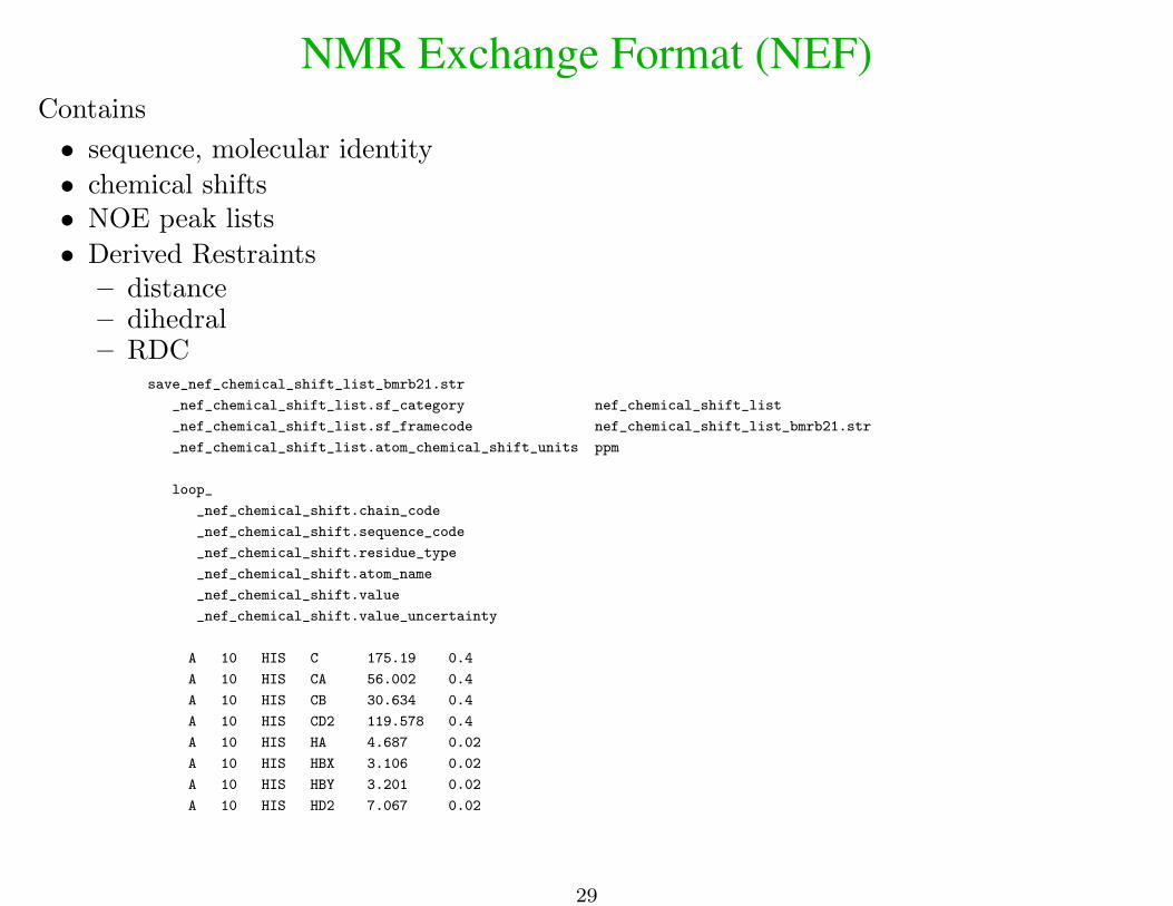
NMR Exchange Format (NEF)Contains

• sequence, molecular identity

• chemical shifts• NOE peak lists

• Derived Restraints– distance– dihedral– RDC

save_nef_chemical_shift_list_bmrb21.str

_nef_chemical_shift_list.sf_category nef_chemical_shift_list

_nef_chemical_shift_list.sf_framecode nef_chemical_shift_list_bmrb21.str

_nef_chemical_shift_list.atom_chemical_shift_units ppm

loop_

_nef_chemical_shift.chain_code

_nef_chemical_shift.sequence_code

_nef_chemical_shift.residue_type

_nef_chemical_shift.atom_name

_nef_chemical_shift.value

_nef_chemical_shift.value_uncertainty

A 10 HIS C 175.19 0.4

A 10 HIS CA 56.002 0.4

A 10 HIS CB 30.634 0.4

A 10 HIS CD2 119.578 0.4

A 10 HIS HA 4.687 0.02

A 10 HIS HBX 3.106 0.02

A 10 HIS HBY 3.201 0.02

A 10 HIS HD2 7.067 0.02

29

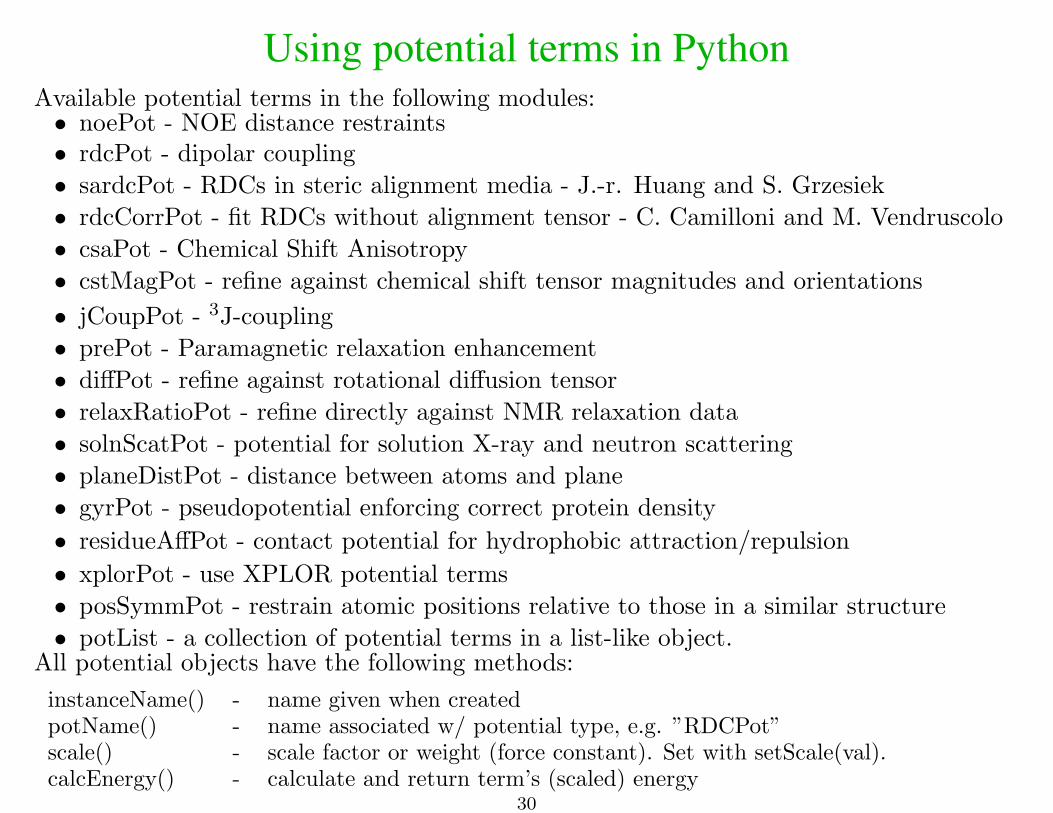
Using potential terms in PythonAvailable potential terms in the following modules:• noePot - NOE distance restraints• rdcPot - dipolar coupling

• sardcPot - RDCs in steric alignment media - J.-r. Huang and S. Grzesiek

• rdcCorrPot - fit RDCs without alignment tensor - C. Camilloni and M. Vendruscolo

• csaPot - Chemical Shift Anisotropy

• cstMagPot - refine against chemical shift tensor magnitudes and orientations

• jCoupPot - 3J-coupling

• prePot - Paramagnetic relaxation enhancement

• diffPot - refine against rotational diffusion tensor

• relaxRatioPot - refine directly against NMR relaxation data

• solnScatPot - potential for solution X-ray and neutron scattering

• planeDistPot - distance between atoms and plane

• gyrPot - pseudopotential enforcing correct protein density

• residueAffPot - contact potential for hydrophobic attraction/repulsion

• xplorPot - use XPLOR potential terms

• posSymmPot - restrain atomic positions relative to those in a similar structure

• potList - a collection of potential terms in a list-like object.All potential objects have the following methods:

instanceName() - name given when createdpotName() - name associated w/ potential type, e.g. ”RDCPot”scale() - scale factor or weight (force constant). Set with setScale(val).calcEnergy() - calculate and return term’s (scaled) energy

30

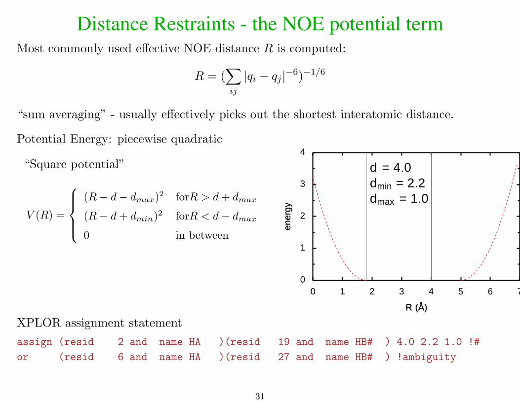
Distance Restraints - the NOE potential termMost commonly used effective NOE distance R is computed:

R = (∑ij

|qi − qj |−6)−1/6

“sum averaging” - usually effectively picks out the shortest interatomic distance.

Potential Energy: piecewise quadratic

“Square potential”

V (R) =

(R− d− dmax)2 forR > d+ dmax

(R− d+ dmin)2 forR < d− dmax0 in between

d = 4.0dmin = 2.2dmax = 1.0

0

1

2

3

4

ener

gyen

ergy

0 1 2 3 4 5 6 7

R (A)R (A)

XPLOR assignment statement

assign (resid 2 and name HA )(resid 19 and name HB# ) 4.0 2.2 1.0 !#

or (resid 6 and name HA )(resid 27 and name HB# ) !ambiguity

31

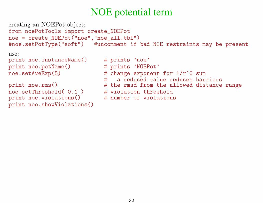
NOE potential termcreating an NOEPot object:from noePotTools import create_NOEPotnoe = create_NOEPot("noe","noe_all.tbl")#noe.setPotType("soft") #uncomment if bad NOE restraints may be present

use:print noe.instanceName() # prints ’noe’print noe.potName() # prints ’NOEPot’noe.setAveExp(5) # change exponent for 1/r^6 sum

# a reduced value reduces barriersprint noe.rms() # the rmsd from the allowed distance rangenoe.setThreshold( 0.1 ) # violation thresholdprint noe.violations() # number of violationsprint noe.showViolations()

32

Residual Dipolar Couplings

+

+

+

+

+

+

+

+

+

+

+

+

+

+

+

+

+

+

+

+

+

+

+

+

B

partial alignment in aligning medium

33

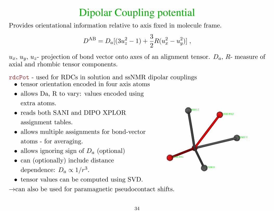
Dipolar Coupling potentialProvides orientational information relative to axis fixed in molecule frame.

DAB = Da[(3u2z − 1) +

3

2R(u2

x − u2y)] ,

ux, uy, uz- projection of bond vector onto axes of an alignment tensor. Da, R- measure ofaxial and rhombic tensor components.

rdcPot - used for RDCs in solution and ssNMR dipolar couplings• tensor orientation encoded in four axis atoms

• allows Da, R to vary: values encoded using

extra atoms.

• reads both SANI and DIPO XPLOR

assignment tables.

• allows multiple assignments for bond-vector

atoms - for averaging.

• allows ignoring sign of Da (optional)

• can (optionally) include distance

dependence: Da ∝ 1/r3.

• tensor values can be computed using SVD.

ANI500:Y

ANI500:PA2

ANI500:Z

ANI500:PA1

ANI500:X

→can also be used for paramagnetic pseudocontact shifts.

34

How to use the rdcPot potentialfrom varTensorTools import create_VarTensor, calcTensor, calcTensorOrientationptensor = create_VarTensor(’phage’) #create a tensor object

ptensor.setDa(7.8) #set initial tensor Da, rhombicityptensor.setRh(0.3)ptensor.setFreedom(’varyDa, varyRh’) #allow Da, Rh to vary

from rdcPotTools import create_RDCPotrdcNH = create_RDCPot("NH",oTensor=ptensor,file=’NH.tbl’)

calcTensor(ptensor) #calc tensor parameters from current structure#using SVD

calcTensorOrientation(ptensor) #calc tensor orientation (with fixed Da, Rh)#from current structure using SVD

NOTE: no need to introduce psf files or coordinates for axis/parameter atoms- this isautomatic.

analysis, accessing potential values:print rdcNH.rms(), rdcNH.violations() # calculates and prints rms, violationsprint ptensor.Da(), ptensor.Rh() # prints these tensor quantitiesrdcNH.setThreshold(0) # violation thresholdprint rdcNH.showViolations() # print out list of violated termsfrom rdcPotTools import Rfactorprint Rfactor(rdcNH) # calculate and print a quality factor

35

RDCPot: additional detailsusing multiple media:btensor=create_VarTensor(’bicelle’)rdcNH_2 = create_RDCPot("NH_2",tensor=btensor,file=’NH_2.tbl’)#[ set initial tensor parameters ]btensor.setFreedom(’fixAxisTo phage’) #orientation same as phage

#Da, Rh vary

multiple expts. single medium:rdcCAHA = create_RDCPot("CAHA",oTensor=ptensor,file=’CAHA.tbl’)

rdcCAHA is a new potential term using the same alignment tensor as rdcNH.

Normally, experiments are normalized to NH Da values.from rdcPotTools import scale_toNHscale_toNH(rdcCAHA,’CAHA’) #rescales RDC prefactor relative to NH

# includes gyromagnetic ratios and# bond lengths

Sign convention: the default is to consider the 15N gyromagnetic ratio to be positive, i.e.the sign of NH experiments is flipped in the input tables. If you do not follow thisconvention, place the following at the beginning of your script:from rdcPotTools import correctGyromagneticSignscorrectGyromagneticSigns()

Scaling convention: scale factor of non-NH terms is determined using the experimentalerror relative to the NH term:rdcCAHA.setScale( (5/2)**2 )# inverse error ^^^ in expt. measurement relative to that for NH

Note: the square well potential is only used for nonbonded (e.g. H-H) experiments.

36

RDCs in Steric Alignment MediaWhen alignment is due solely to molecular shape.from sardcPotTools import create_SARDCPot

sardc = create_SARDCPot("saRDC","NH.tbl")J.-R. Huang and S. Grzesiek, “Ensemble calculations ofunstructured proteins constrained by RDC and PRE data: a casestudy of urea-denatured ubiquitin,” J. Am. Chem. Soc. 132,694-705 (2010).

• Important for ensemble calculations where RDCPot leads to underdeterminedalignment tensors.

• Input tables are the same format used in RDCPot.

One can extract a traditional Xplor-NIH alignment tensor:from varTensorTools import saupeToVarTensorfrom sardcPotTools import saupeMatrix

#generate a VarTensor representation of the SARDC alignment tensormedium = saupeToVarTensor( saupeMatrix(sardc),dmax )

print medium.Rh() #print rhombicity

37

Chemical Shift Anisotropy potentialProvides additional orientational information from the full chemical shift tensor frommeasurements in an aligning medium.

∆δ =∑i,j

Aiσj cos2(θi,j)

Ai - a principal moment of the alignment tensorσj - a principal moment of the CSA tensor

θi,j - angle between the ith orientation tensor principal axis and the jth CSA tensorprincipal axis.

How to use the csaPot potentialfrom csaPotTools import create_CSAPotcsaP = create_CSAPot(name,oTensor=tensor,file=’csaP.tbl’)

csaP.setDaScale( val ) # s.t. can be used with RDC alignment tensorcsaP.setScale( forceConstant )calcTensor(tensor) #use if the structure is approximately correct

NOTE: create_CSAPot uses built-in values for the chemical shift tensor. Alternate valuescan be specified by modifying csaPotTools.csaData.

→can be used with ssNMR CSA or chemical shift tensor data.

38

J-coupling potentialKarplus relationship

3J = A cos2(θ + θ∗) +B cos(θ + θ∗) + C,

θ is a torsion angle, defined by four atoms.A, B, C and θ∗ are set using the COEF statement in the j-coupling assignment table (orusing object methods).

Use in Pythonfrom jCoupPotTools import create_JCoupPot# set Karplus parameters while creating the potential term.

jCoup = create_JCoupPot("hnha","jna_coup.tbl",A=15.3,B=-6.1,C=1.6,phase=0)

analysis:print Jhnha.rms()print Jhnha.violations()print Jhnha.showViolations()

39

Paramagnetic Relaxation Enhancement

Γ = SAB(τc)r−6AB,

rAB - distance between paramagnetic center and amide proton.

SAB(τc) - function of correlation time τc.

from prePotTools import create_PREPotpre = create_PREPot("pre","file.tbl",

eSpinQuantumNumber=2.5,freq=500, # Larmor frequency in MHztauc=3.0, # correlation time in nsfixTau=True)

potList.append(pre)

• uses modified Solomon-Bloembergen Eq. which can account for tag motion andmultiple tag conformations.

• can simultaneously determine correlation time.

Example in eginput/pre/refine/newRefine.py

Iwahara, et. al. JACS 126, 5879 (2004).

[in old XPLOR interface: PMAG term - Donaldson, et. al. JACS 123, 9843 (2001).]

40

Solvent Paramagnetic Relaxation Enhancement dataEmpirical relationship:

ΓsPRE ≈ ASAcc +B

with effective surface area:

SAcc ≈(∑

i

r−2i

)−1

ri is distance of amide proton in question to a heavy atom, and the sum is over all heavyatoms.

from nbTargetPotTools import create_NBTargetPot, calibratepsol = create_NBTargetPot(’psol’,’file.tbl’,restraintFormat=’xplor’)#psol.setPotType("correlation")calibrate(psol) # determine A and B by fit to experimentpotList.append(psol)

also used to describe solvent NOE.

Wang, et. al. J. Magn. Res. 221, 76 (2012).

Another, more rigorous term available, not yet published.

41

Use of Relaxation Data in Structure CalculationYaroslav Ryabov

Ratio of transverse to longitudinal relaxation rates: ρ = R2/R1 contains information onbond vector orientation relative to a diffusion tensor.

The diffusion tensor can be computed from atomic coordinates.

Thus: relaxation data can be used to obtain bond vector and overall shape information.

# read in relaxation data from file relax.dat# data format specified by tablePatternfrom diffPotTools import readInRelaxData, mergeRelaxData, make_ratiorelax_data = readInRelaxData("relax.dat",

pattern=tablePattern,verbose=True)

from diffPotTools import make_ratiofor item in relax_data: make_ratio(item)

from relaxRatioPotTools import create_RelaxRatioPotpot =create_RelaxRatioPot(’relax’,

data_in = relax_data,freq = freq, #spectrometer freqtemperature =temperature, # expt. temp.)

42

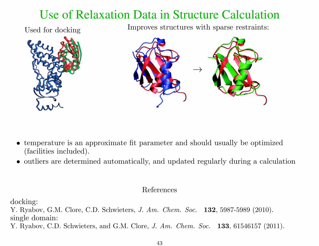
Use of Relaxation Data in Structure CalculationUsed for docking Improves structures with sparse restraints:

→

• temperature is an approximate fit parameter and should usually be optimized(facilities included).

• outliers are determined automatically, and updated regularly during a calculation

References

docking:Y. Ryabov, G.M. Clore, C.D. Schwieters, J. Am. Chem. Soc. 132, 5987-5989 (2010).single domain:Y. Ryabov, C.D. Schwieters, and G.M. Clore, J. Am. Chem. Soc. 133, 61546157 (2011).

43

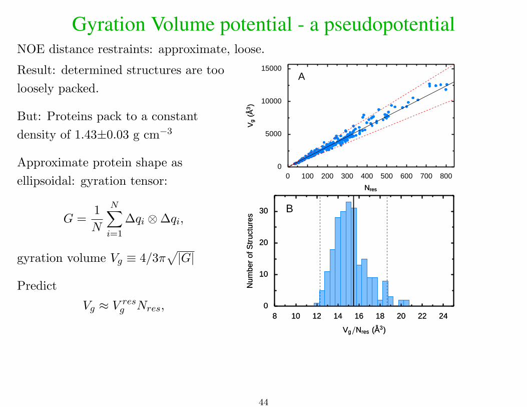
Gyration Volume potential - a pseudopotentialNOE distance restraints: approximate, loose.

Result: determined structures are too

loosely packed.

But: Proteins pack to a constant

density of 1.43±0.03 g cm−3

Approximate protein shape as

ellipsoidal: gyration tensor:

G =1

N

N∑i=1

∆qi ⊗∆qi,

gyration volume Vg ≡ 4/3π√|G|

Predict

Vg ≈ V resg Nres,

A

0

5000

10000

15000

Vg

(A3)

Vg

(A3)

0 100 200 300 400 500 600 700 800

NresNres

B

0

10

20

30

Num

ber

ofS

truc

ture

sN

umbe

rof

Str

uctu

res

8 10 12 14 16 18 20 22 24

Vg/Nres (A3)Vg/Nres (A3)

0

10

20

30

8 10 12 14 16 18 20 22 24

44

The Vg potential

Egyr = wgyr(w(1)gyrEp(Vg − V res

g ; 0)

+w(2)gyrEp(Vg − V res

g ; ∆Vg))

Ep(x,∆x) =

(x−∆x)2 for x > ∆x

(x+ ∆x)2 for x < −∆x

0 otherwise

Example of use of this term:from gyrPotTools import create_GyrPotgyr = create_GyrPot(’Vgyr’,’not resname ANI’)potList.append(gyr)

Reference: C.D. Schwieters and G.M. Clore, J. Phys. Chem. B 112, 6070-6073 (2008).

45

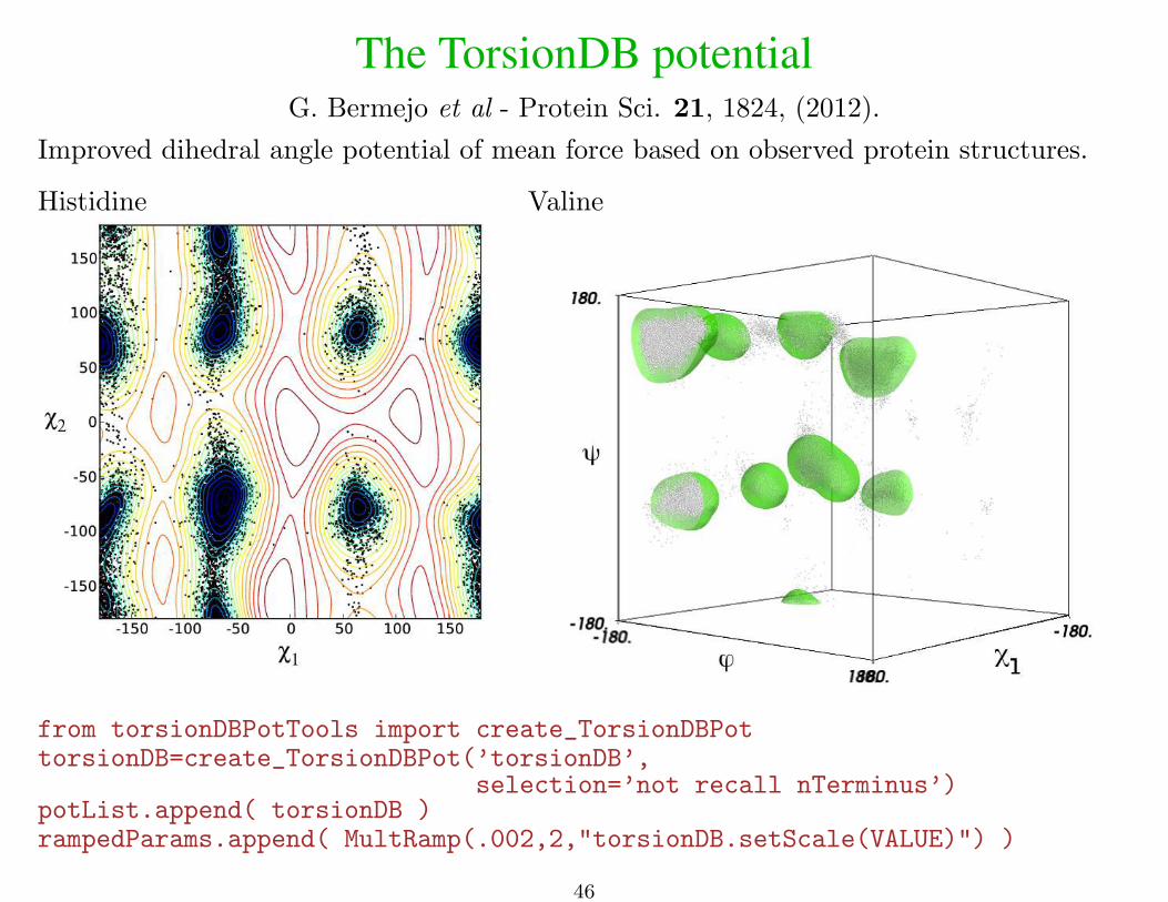
The TorsionDB potentialG. Bermejo et al - Protein Sci. 21, 1824, (2012).

Improved dihedral angle potential of mean force based on observed protein structures.

Histidine Valine

from torsionDBPotTools import create_TorsionDBPottorsionDB=create_TorsionDBPot(’torsionDB’,

selection=’not recall nTerminus’)potList.append( torsionDB )rampedParams.append( MultRamp(.002,2,"torsionDB.setScale(VALUE)") )

46

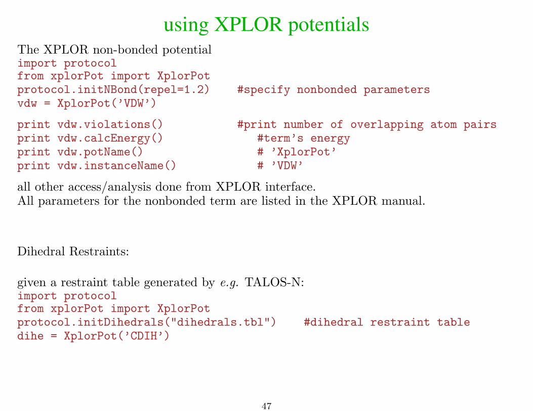
using XPLOR potentialsThe XPLOR non-bonded potentialimport protocolfrom xplorPot import XplorPotprotocol.initNBond(repel=1.2) #specify nonbonded parametersvdw = XplorPot(’VDW’)

print vdw.violations() #print number of overlapping atom pairsprint vdw.calcEnergy() #term’s energyprint vdw.potName() # ’XplorPot’print vdw.instanceName() # ’VDW’

all other access/analysis done from XPLOR interface.All parameters for the nonbonded term are listed in the XPLOR manual.

Dihedral Restraints:

given a restraint table generated by e.g. TALOS-N:import protocolfrom xplorPot import XplorPotprotocol.initDihedrals("dihedrals.tbl") #dihedral restraint tabledihe = XplorPot(’CDIH’)

47

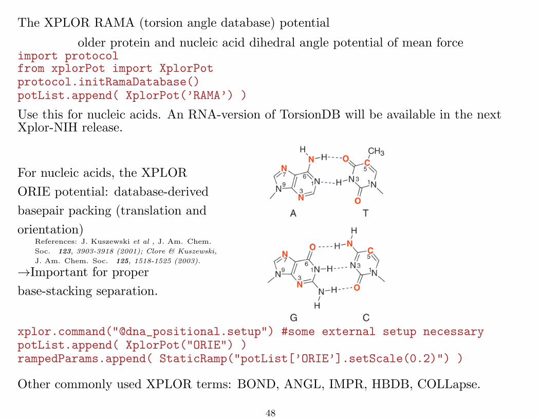
The XPLOR RAMA (torsion angle database) potential

older protein and nucleic acid dihedral angle potential of mean forceimport protocolfrom xplorPot import XplorPotprotocol.initRamaDatabase()potList.append( XplorPot(’RAMA’) )

Use this for nucleic acids. An RNA-version of TorsionDB will be available in the nextXplor-NIH release.

For nucleic acids, the XPLOR

ORIE potential: database-derived

basepair packing (translation and

orientation)References: J. Kuszewski et al , J. Am. Chem.

Soc. 123, 3903-3918 (2001); Clore & Kuszewski,

J. Am. Chem. Soc. 125, 1518-1525 (2003).

→Important for proper

base-stacking separation.

xplor.command("@dna_positional.setup") #some external setup necessarypotList.append( XplorPot("ORIE") )rampedParams.append( StaticRamp("potList[’ORIE’].setScale(0.2)") )

Other commonly used XPLOR terms: BOND, ANGL, IMPR, HBDB, COLLapse.

48

using XPLOR potentialsExample using a Radius of Gyration (COLLapse) potentialimport protocolfrom xplorPot import XplorPot

#helper setup functionprotocol.initCollapse(’resid 3:72’) #specify globular portion

# GyrPot (gyration volume) can be# used for non-globular domains

rGyr = XplorPot(’COLL’)xplor.command(’collapse scale 0.1 end’) #manipulate in XPLOR interface

default target=2.2 ∗N0.38res − 1

(empirical relationship for compact globular proteins)

accessing associated valuesprint rGyr.calcEnergy() #term’s energyprint rGyr.potName() # ’XplorPot’print rGyr.instanceName() # ’COLL’

all other access/analysis done from XPLOR interface.

49

using XPLOR potentialsother terms have no Python helpers, and must be configured via the XPLOR interface.

XRay Diffractionxplor.command(r’’’xref

.

.

.end’’’)potList.append( XplorPot("xref") )

Fiber XRay Diffractionxplor.command(r’’’fiber

.

.

.end’’’)potList.append( XplorPot("xref") )

References:R.C. Denny et al , Fibre Diffr. Rev 6, 30-33 (1997) ; H. Wang and G.

Stubbs, Acta Cryst A49, 504-513 (1993).

50

Collections of potentials - PotListpotential term which is a collection of potentials:from potList import PotListpots = PotList()pots.append(noe); pots.append(Jhnha); pots.append(gyr)pots.calcEnergy() # total energy

nested PotLists:rdcs = PotList(’rdcs’) #convenient to collect like termsrdcs.append( rdcNH ); rdcs.append( rdcNH_2 )rdcs.setScale( 0.5) #set overall scale factorpots.append( rdcs )for pot in pots: #pots looks like a Python list

print pot.instanceName()

noehnhaCOLLrdcs

51

Implementing a new potential term - in Pythonfrom pyPot import PyPot ; from vec3 import norm, Vec3class BondPot(PyPot):

’’’ example class to evaluate energy, derivs of a single bond’’’def __init__(self,name,atom1,atom2,length,forcec=1):

’’’ constructor - force constant is optional.’’’PyPot.__init__(self,name) #first call base class constructorself.a1 = atom1 ; self.a2 = atom2self.length = length; self.forcec = forcecreturn

def calcEnergy(self):self.q1 = self.a1.pos() ; self.q2 = self.a2.pos()self.dist = norm(self.q1-self.q2)return 0.5 * self.scale() * self.forcec * (self.dist-self.length)**2

def calcEnergyAndDerivList(self,derivs):energy = self.calcEnergy()deriv1 = Vec3(map(lambda x,y:x*y,

[self.forcec * (self.dist-self.length) / self.dist]*3 ,( self.q1[0]-self.q2[0],

self.q1[1]-self.q2[1],self.q1[2]-self.q2[2] )))

derivs[self.a1] = self.scale() *deriv1derivs[self.a2] = -self.scale() * deriv1return energy

pass

to use:p = BondPot(’bond’,AtomSel(’resid 1 and name C’)[0],

AtomSel(’resid 1 and name O’)[0], length=1.5)

52

The IVM (internal variable module)Used for dynamics and minimization

in biomolecular NMR structure determination, many internal coordinates are known orpresumed to take usual values:

• bond lengths, angles- take values from high-resolution crystal structures.

• aromatic amino acid side chain regions - assumed rigid.

• nucleic acid base regions - assumed rigid.

• refinement against RDC data can’t distort covalent geometry.

• non-interfacial regions of protein and nucleic acid complexes (component structuresmay be known- only interface needs to be determined)

Can we take advantage of this knowledge (find the minima more efficiently)?

• can take larger MD timesteps (without high freq bond stretching)

• configuration space to search is smaller:Ntorsion angles ∼ 1/9 NCartesian coordinates

• don’t have to worry about messing up known coordinates.

53

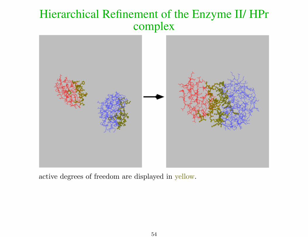
Hierarchical Refinement of the Enzyme II/ HPrcomplex

active degrees of freedom are displayed in yellow.

54

MD in internal coordinates is nontrivialConsider Newton’s equation:

F = Ma

for MD, we need a, the acceleration in internal coordinates, given forces F .Problems:

• express forces in internal coordinates

• solve the equation for a.

In Cartesian coordinates a is (vector of) atomic accelerations. M is diagonal.

In internal coordinates M is full and varies as a function of time: solving for a scales asN3

internal coordinates.

Solution: comes to us from the robotics community. Involves clever solution of Newton’sequation: The molecule is decomposed into a tree structure, a is solved for by iteratingfrom trunk to branches, and backwards.

Xplor-NIH implementation: C.D. Schwieters and G.M. Clore; J. Magn. Reson. 152, 288-302 (2001).A copy of the IVM paper with some corrections is available athttp://nmr.cit.nih.gov/xplor-nih/doc/intVar.pdf

55

Tree Structure of a Molecule

TYR3:CG

TYR3:CD1

1a

2a

3a

4a

5a

6a

7a

8a

9a

10a

11a

12a13a

14a

15a

16a

8b

11b

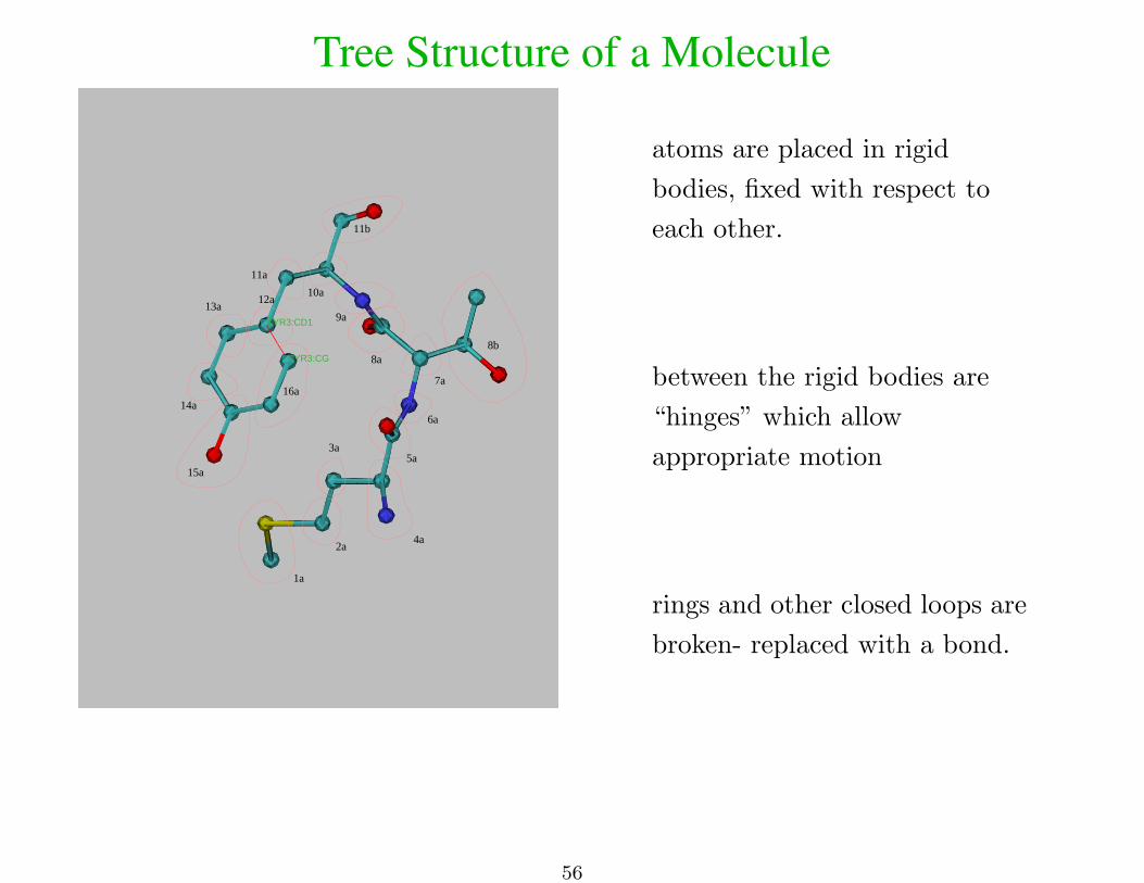
atoms are placed in rigid

bodies, fixed with respect to

each other.

between the rigid bodies are

“hinges” which allow

appropriate motion

rings and other closed loops are

broken- replaced with a bond.

56

Topology Setuptorsion angle dynamics with fixed region:

from ivm import IVMintegrator = IVM() #create an IVM objectintegrator.fix( AtomSel("resid 100:120") ) # these atoms are fixed in spaceintegrator.group( AtomSel("resid 130:140") ) # fix relative to each other,

# but translate, rotate in space

from protocol import torsionTopologytorsionTopology(integrator) # group rigid side chain regions

# break proline rings# group and setup all remaining# degrees of freedom for# torsion angle dynamics## topology setup of pseudoatoms# e.g. alignment tensor atoms:# - tensor axis should rotate# only - not translate.# - only single dof of Da and Rh# parameter atoms is significant.

57

IVM Implementation details:other coordinates also possible: e.g. mixing Cartesian, rigid body and torsion anglemotions.

convenient features:

• variable-size timestep algorithm

• will also perform minimization

• facility to constrain bonds which cause loops in tree.

full example script in eginput/gb1_rdc/refine.py of the Xplor-NIH distribution.

Dynamics with variable timestepimport protocolbathTemp=2000protocol.initDynamics(ivm=integrator, #note: keyword arguments

bathTemp=bathTemp,finalTime=1, # use variable timestepprintInterval=10, # print info every ten stepspotList=pots)

integrator.run() #perform dynamics

58

High-Level Helper ClassesAnnealIVM: perform simulated annealingfrom simulationTools import AnnealIVManneal= AnnealIVM(initTemp =3000, #high initial temperature

finalTemp=25, #final temperaturetempStep =25, # temperature incrementivm=integrator, # ivm object used for molecular dynamicsrampedParams = coolParams) #list of energy parameters to scale

anneal.run() # actually perform simulated annealing

Force constants of some terms are geometrically scaled during refinement: duringsimulated annealing step n of N , the force constant is

k(n) = γnk(0)

• k(0) and k(N) - initial and final force constants

• γN = k(N)/k(0)

from simulationTools import MultRamp #multiplicatively ramped parametercoolParams=[]coolParams.append( MultRamp(2,30, #change NOE scale factor

"noe.setScale( VALUE )") )

59

StructureLoop: calculate multiple structuresfrom simulationTools import StructureLoopStructureLoop(structureNums=range(10), # calculate 10 structures

structLoopAction=calcStructure, # calcStructure is functionpdbTemplate=pdbTemplate) # template for output structures

pdbTemplate = ’SCRIPT_STRUCTURE.sa’#SCRIPT -> replaced with the name of the input script (e.g. ’anneal.py’)#STRUCTURE -> replaced with the number of the current structure

StructureLoop also helps with analysis:from simulationTools import StructureLoop, FinalParamsStructureLoop(structureNums=range(10),

structLoopAction=calcStructure,pdbTemplate=outFilename,pdbFilesIn="file_*.pdb" # specify input filesdoWriteStructures=True, # after calcStructure, write structure, violsaverageTopFraction=0.5, # fraction of structures to useaverageFitSel="not hydro", #atoms used for fitting structuresaveragePotList=potList, #terms to use to compute of ave. structaverageContext=FinalParams(rampedParams), #force constants usedaverageFilename="ave.pdb", #output filenamegenViolationStats=True, # generate a .stats file with

# energy/violation/structure stats).run()

StructureLoop transparently takes care of parallel structure calculation.

60

Parallel computation of multiple structuresComputation of multiple structures with different initial velocities and/or coordinates:gives idea of structure precision, convergence of calculation.

on a multi-processor computer:xplor -smp <number of CPUs> -py ...

on a cluster running PBS: [Supported implementations: PBSPro and Torque]pbsxplor -l nodes=<number of nodes> -py ...

on a cluster running SLURM: [use this on Biowulf]slurmXplor -py -nodes < num > [options] script.py

on a Scyld clusterxplor -scyld <number of CPUs> -py ...

or manual node specificationxplor -parallel -machines <machine file> -py ...

convenient Xplor-NIH parallelization• spawns multiple versions of xplor on multiple machines via ssh or rsh.• structure and log files collected in the current local directory.• robust to crashing compute nodes, crashing XPLOR runs, and the presence of dead

nodesrequirements:• ability to login to remote nodes via ssh or rsh, without password• shared filesystem which looks the same to each node

• fully populated /bin and /usr/bin directories.

following environment variables set: XPLOR NUM PROCESSES, XPLOR PROCESS

61

Integrative Approaches to Structure CalculationCombine multiple sources of data

Combine NMR data with

• Solution Scattering - SAXS, SANS

• Cryo-EM

• X-ray crystallogaphy

• Fiber Diffraction

• EPR

62

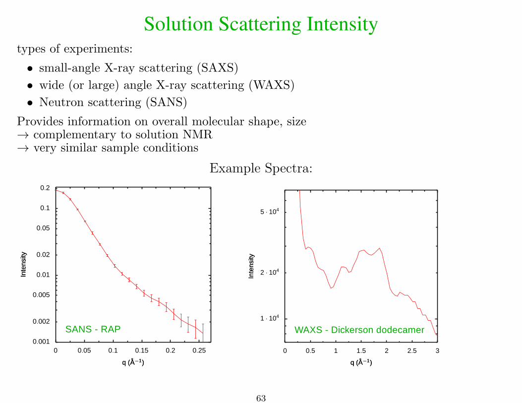
Solution Scattering Intensitytypes of experiments:

• small-angle X-ray scattering (SAXS)

• wide (or large) angle X-ray scattering (WAXS)

• Neutron scattering (SANS)

Provides information on overall molecular shape, size→ complementary to solution NMR→ very similar sample conditions

Example Spectra:

SANS - RAP0.001

0.002

0.005

0.01

0.02

0.05

0.1

0.2

Inte

nsity

Inte

nsity

0 0.05 0.1 0.15 0.2 0.25

q (A−1)q (A−1)

WAXS - Dickerson dodecamer1 · 104

2 · 104

5 · 104

Inte

nsity

Inte

nsity

0 0.5 1 1.5 2 2.5 3

q (A−1)q (A−1)

63

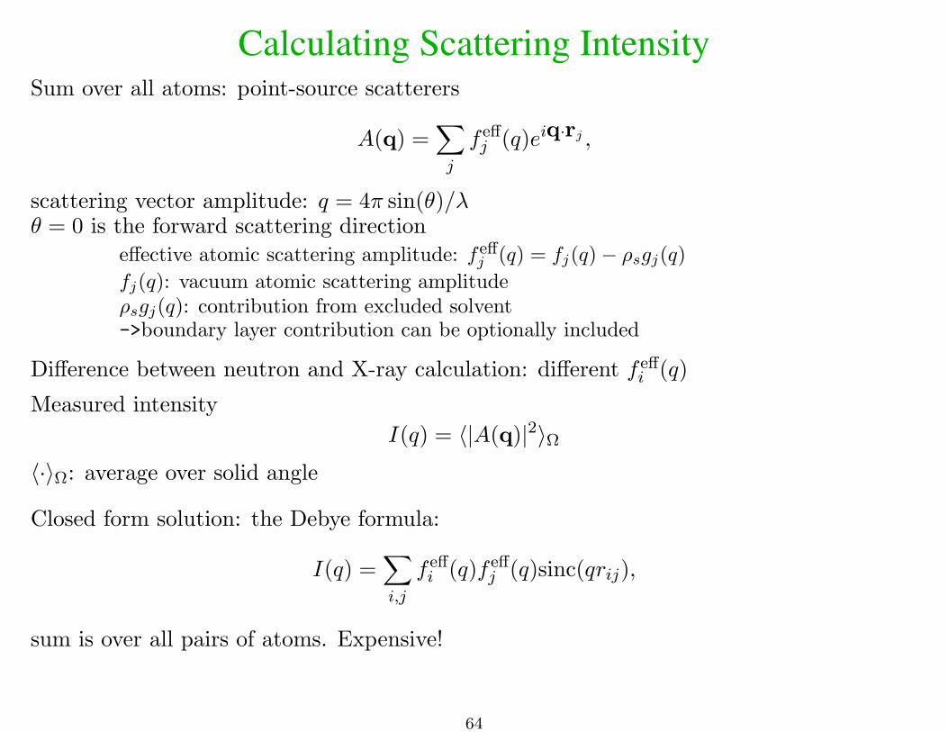
Calculating Scattering IntensitySum over all atoms: point-source scatterers

A(q) =∑j

f effj (q)eiq·rj ,

scattering vector amplitude: q = 4π sin(θ)/λθ = 0 is the forward scattering direction

effective atomic scattering amplitude: feffj (q) = fj(q)− ρsgj(q)

fj(q): vacuum atomic scattering amplitudeρsgj(q): contribution from excluded solvent->boundary layer contribution can be optionally included

Difference between neutron and X-ray calculation: different f effi (q)

Measured intensity

I(q) = 〈|A(q)|2〉Ω〈·〉Ω: average over solid angle

Closed form solution: the Debye formula:

I(q) =∑i,j

f effi (q)f eff

j (q)sinc(qrij),

sum is over all pairs of atoms. Expensive!

64

Scattering Intensity Approximations

Instead, compute A(q) on a sphere and integrate

over solid angle numerically.

Points are selected quasi-uniformly on the sphere

using the Spiral algorithm:

Additionally, combine atoms in “globs”:

fglob(q) = [∑i,j

f effi (q)f eff

j (q)sinc(qrij)]1/2,

Correct globbing, numerical integration errors with a multiplicative q-dependentcorrection factor ccorrect:

I(q) = ccorrect(q)Iapprox(q),

65

Calculated intensity for DNA scattering: numerical and globbing approximations:

5 · 103

1 · 104

2 · 104

5 · 104

Inte

nsity

Inte

nsity

0 0.5 1 1.5 2 2.5 3

q (A−1)q (A−1)

exact100 points on sphere100 points on sphere - using globs

66

Boundary layer contributionBound water contributes to the scattering amplitude.

Model as a layer of uniform thickness around the molecular structure with density ρb.

• Use the Varshneya algorithm to efficiently generate an

outer surface: roll solvent molecule over atoms whose

radii are increased by rb.

• Inner surface is generated using the points and surface

normals.

• Each voxel defined by the tesselization procedure

contributes to the scattering amplitude:∑k

f sph(q; rk)eiq·yk ,

with

f sph(q; rk) = ρb4π/q2[sin(qrk)/q − rk cos(qrk)]

aA. Varshney, F.P. Brooks, W.V. Wright, IEEE Comp. Graphics App.14, 19-25 (1994)

Alternate fit procedure available if buffer subtraction is significant source of error.

67

Determining Solvent Scattering Parametersas in Crysola three parameters are fit

Effective atomic scattering amplitude:

f effj (q) = fj(q)− ρsgj(q),

fj(q): vacuum atomic scattering

amplitude

ρs: bulk solvent electron density

amplitude due to excluded solvent:

gj(q) = sV Vj exp(−πq2V2/3j )×

exp[−π(qrm)2(4π/3)2/3(sr2 − 1)]

Vj : atomic volume

rm: is the radius corresponding to the

average atomic volume

sV , sr: scale factors to be fit.

Bound solvent scattering amplitude

f sph(q; rk) = ρb4π/q2[ sin(qrk)/q −

rk cos(qrk)]

ρb: boundary layer electron density

rk: radius corresponding to voxel

volume.

three parameters are fit using a grid search.

For SANS: one additional parameter: isotropic background added to calculated I(q).aD. Svergun, C. Barberato and M.H.J. Koch, J. Appl. Cryst. 28, 768-773 (1995).

68

Solution Scattering of Rigid BodiesFor atoms within a rigid body, the relative atom positions do not change, so after aninitial calculation the corresponding contribution to the scattering amplitude can becomputed without referring to atomic positions. If r′j is the atomic position of atom j

after displacement of the rigid body with initial posistion given by rj , then

r′j = Rrj + ∆r,

where R and ∆r, respectively, describe the rotation and translation of the rigid body, thecorresponding rigid body scattering amplitude is:

Arigid(q; r) = ei∆r·qA0rigid(q′; r),

where r denotes the dependence on the set of initial atomic coordinates and

q′ = RTq.

In practice, Arigid(q; r) is computed using a spline over a spherical surface of constant q

to evaluate A0rigid(q′; r), the scattering amplitude at initial atomic position, but rotated

scattering vector amplitude, q′.

The use of this expression yields vast speedups when a calculation can be decomposedinto a small number of rigid bodies, as it becomes independent of the number of atoms.

69

Refinement against solution scattering dataRefinement target function

Escat = wscat

∑j

ωj(I(qj)− Iobs(qj))2,

wscat, ωj : weight factors

Typically set ωj = 1/∆Iobs(qj)2 - inverse square of error. → so Escat ∼ χ2.

• Correction factor ccorrect periodically recomputed.

• Non-zero scattering contribution from surface-bound solvent- periodically computed,effect included in ccorrect

• Rigid subunits’ scattering contribution computed very efficiently during dynamics,minimization.• Buffer background subtraction can be included usingsolnScatPotTools.fitSolventBuffer.• SANS data is also supported

70

Example Xplor-NIH SAXS setupfrom solnXRayPotTools import create_solnXRayPotimport solnXRayPotToolsxray=create_solnXRayPot(’xray’,

experiment=’saxs.dat’,numPoints=26,normalizeIndex=-3,preweighted=False)

xrayCorrect=create_solnXRayPot(’xray-c’,experiment=saxs.dat’,numPoints=26,normalizeIndex=-3,preweighted=False)

solnXRayPotTools.useGlobs(xray)xray.setNumAngles(50)xrayCorrect.setNumAngles(500)potList.append(xray)crossTerms.append(xrayCorrect)

#corrects I(q) for globbing, small angular grid and# includes solvent contribution correctionsfrom solnScatPotTools import fitParamsrampedParams.append( StaticRamp("fitParams(xrayCorrect)") )rampedParams.append(StaticRamp("xray.calcGlobCorrect(xrayCorrect.calcd())"))

71

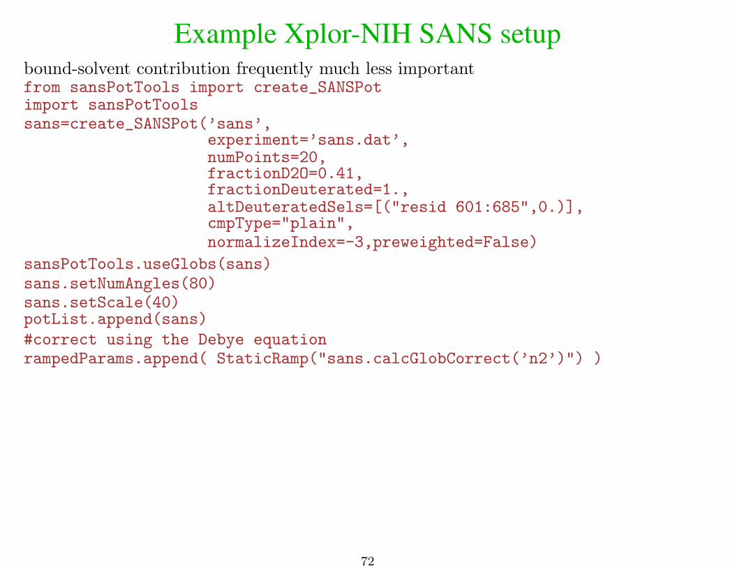
Example Xplor-NIH SANS setupbound-solvent contribution frequently much less importantfrom sansPotTools import create_SANSPotimport sansPotToolssans=create_SANSPot(’sans’,

experiment=’sans.dat’,numPoints=20,fractionD2O=0.41,fractionDeuterated=1.,altDeuteratedSels=[("resid 601:685",0.)],cmpType="plain",normalizeIndex=-3,preweighted=False)

sansPotTools.useGlobs(sans)sans.setNumAngles(80)sans.setScale(40)potList.append(sans)

#correct using the Debye equationrampedParams.append( StaticRamp("sans.calcGlobCorrect(’n2’)") )

72

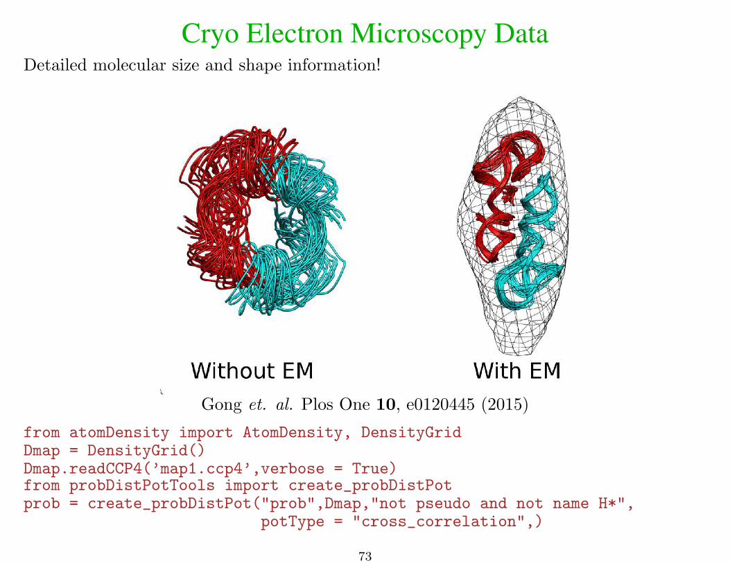
Cryo Electron Microscopy DataDetailed molecular size and shape information!

Gong et. al. Plos One 10, e0120445 (2015)

from atomDensity import AtomDensity, DensityGridDmap = DensityGrid()Dmap.readCCP4(’map1.ccp4’,verbose = True)from probDistPotTools import create_probDistPotprob = create_probDistPot("prob",Dmap,"not pseudo and not name H*",

potType = "cross_correlation",)

73

Cryo EM + NMR: TRPV1 with bound double-knot toxin

Bae et. al. eLife, accepted (2015).

74

Refinement against an ensembleRefinement of DNA 12-mer using NOE, RDC and X-ray scattering data

four calculated structures One four-membered ensemble

75

Refinement against an ensemble

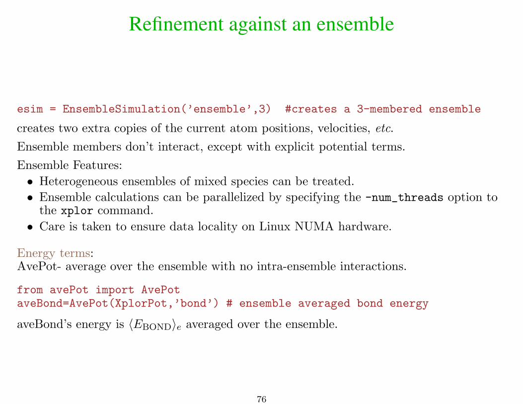
esim = EnsembleSimulation(’ensemble’,3) #creates a 3-membered ensemble

creates two extra copies of the current atom positions, velocities, etc.

Ensemble members don’t interact, except with explicit potential terms.

Ensemble Features:

• Heterogeneous ensembles of mixed species can be treated.

• Ensemble calculations can be parallelized by specifying the -num_threads option tothe xplor command.

• Care is taken to ensure data locality on Linux NUMA hardware.

Energy terms:AvePot- average over the ensemble with no intra-ensemble interactions.

from avePot import AvePotaveBond=AvePot(XplorPot,’bond’) # ensemble averaged bond energy

aveBond’s energy is 〈EBOND〉e averaged over the ensemble.

76

Refinement against an ensembleMost NMR observables must be averaged appropriately- AvePot is not appropriate- itonly averages ensemble energies.

For example, the appropriate RDC value is 〈DAB〉e averaged over the ensemble. The

resulting energy is then E(〈DAB〉e).Most Python energy terms will do proper ensemble averaging. XPLOR terms will not.

Additional potential terms: RAPPot, ShapePot - restrain atom positions within anensemble - so members don’t drift too far apart.

Example: restrain the positions of Cα atoms to be the same in all members of theensemble.

from posRMSDPotTools import RAPPotrap = RAPPot("ncs","name CA") # create termrap.setScale( 100.0 )rap.setPotType( "square" ) # harmonic potential has a flat regionrap.setTol( 0.3 ) # 1/2-width of flat region

77

Can also refine against bond-vector order parameter for ensemble of size Ne, with unitvector ui along the appropriate bond vector in ensemble member i

S2 =1

2N2e

∑ij

(3 cos(ui · uj)2 − 1)

[can use data from e.g. relaxation experiments.]

from orderPot import OrderPotorderPot = OrderPot("s2_nh",open("nh_s2.tbl").read())

and crystallographic temperature factor for atom j in terms of qij , it’s position inensemble i, and it’s ensemble-averaged value qj

Bj = 8π2/Ne

∑i

|qij − qj |2

from posRMSDPotTools import create_BFactorPotbFactor = PotList("bFactor")

78

Variable Ensemble WeightsSetting ensemble weightsesim = EnsembleSimulation(’ensemble’,3)esim.setWeights( [0.2,0.1,0.7] ) # set weights for all ensemble membersnoe = NOEPot(’noe’)noe.setEnsWeights( [0.2,0.1,0.7] ) # set weight for only this NOE term

Ensemble Weights can be optimized during structure calculation.

from ensWeightsTools import create_EnsWeightsensw = create_EnsWeights(’ensw’)ensw.setWeights([0.2,0.2,0.6]) # set the initial/target weights

from sardcPotTools import create_SARDCPotrdc = create_SARDCPot("RDC",restraints=stericRDC)rdc.addEnsWeights(ensw) # specify that this potential term use this set

# of ensemble weights

different potential terms can have different ensemble weights

potList.append(ensw) #potential term biases the weights towards# initial values

Using the EnsWeights energy term avoids situations with zero ensemble weight.

79

Symmetric MultimersMaintain C2 Symmetry

“NCS” term - keep dimer subunits identical

from posDiffPotTools import create_PosDiffPotdiNCS = create_PosDiffPot("diNCS", "segid A", "segid B")potList.append(diNCS)

Distance symmetry to enforce C2 symmetry

from distSymmTools import create_DistSymmPot, genDimerRestraintsdSymm = create_DistSymmPot(’dSymm’)for r in genDimerRestraints(segids=[’A’,’B’],

resids=range(10,150,10)):dSymm.addRestraint(r)pass

dSymm.setShowAllRestraints(True)potList.append(dSymm)

Proper NOE distance calculation for SUM averaging subunit ambiguous restraint: thenMono setting

noe.setNMono(2)

80

Refinement in Explicit Solvent

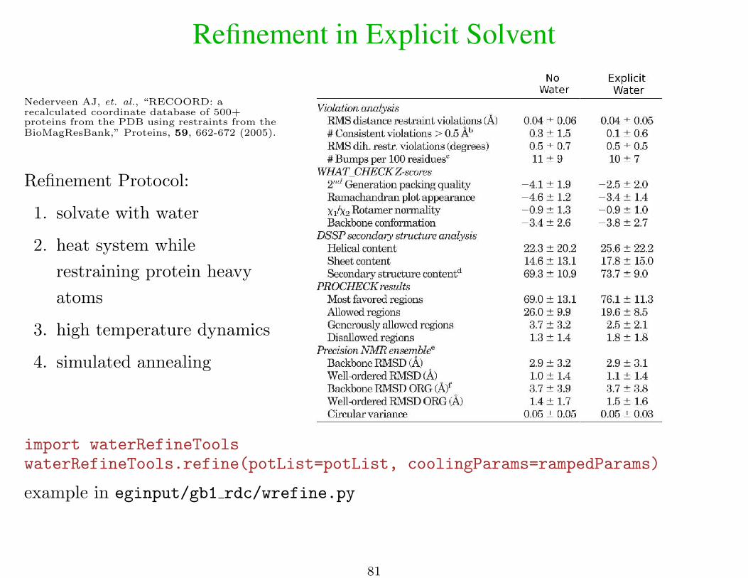
Nederveen AJ, et. al., “RECOORD: arecalculated coordinate database of 500+proteins from the PDB using restraints from theBioMagResBank,” Proteins, 59, 662-672 (2005).

Refinement Protocol:

1. solvate with water

2. heat system while

restraining protein heavy

atoms

3. high temperature dynamics

4. simulated annealing

import waterRefineToolswaterRefineTools.refine(potList=potList, coolingParams=rampedParams)

example in eginput/gb1 rdc/wrefine.py

81

Calculations Using Implicit Solvent: EEFxThe EEFx Implicit Solvent Model

Y. Tian, et. al., “A Practical Implicit SolventPotential for NMR Structure Calculation ,” J. Magn.Res. 243, 54-64 (2014).

Can be used at all stages of

structure determination.

Example in

eginput/gb1 rdc/wrefine.py

Now also includes implicit

membrane potential.

Reference No Solvent Using EEFx

from eefxPotTools import create_EEFxPot, param_LKeefxpot=create_EEFxPot("eefxpot","not name H*",paramSet=param_LK)

82

Implicit Solvent with a membrane: EEFxYe Tian, C.D. Schwieters, S.J. Opella and F.M. Marassi, “A Practical Implicit MembranePotential for NMR Structure Calculations of Membrane Proteins,” Biophys J. 109, 574-585 (2015).

No Membrane Using EEFx+membrane

Example in eginput/eefx/membrane

83

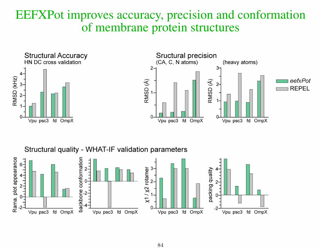
EEFXPot improves accuracy, precision and conformationof membrane protein structures

84

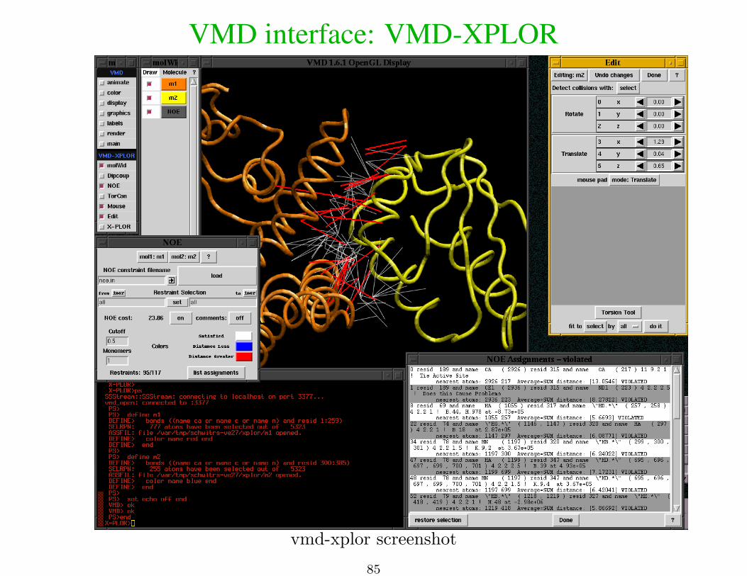
VMD interface: VMD-XPLOR

vmd-xplor screenshot

85

• visualize molecular structures• visualize restraint info• manually edit structures

• generate publication-quality figures

load multiple files at once

% vmd-xplor -noxplor refine*.pdb

command-line invocation of separate Xplor-NIH and VMD-XPLOR jobs:

% vmd-xplor -port 3359 -noxplor% xplor -port 3359 -py

Xplor-NIH snippet to draw bonds between backbone atoms, and labels:import vmdInter

vmd = VMDInter()x = vmd.makeObj("x")x.bonds( AtomSel("name ca or name c or name n") )label = vmd.makeObj("label")label.labels( AtomSel("name ca") )

86

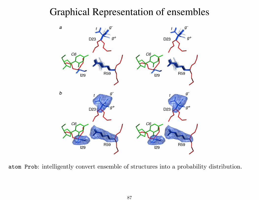
Graphical Representation of ensembles

atom Prob: intelligently convert ensemble of structures into a probability distribution.

87

The PASD facility for automatic NOE assignmentdeveloped by John Kuszewski

sometimes referred to as Marvin

main features:

• implemented in TCL interface.

• initial assignment likelihoods set by topological network of interconnected distancerestraints.• probabilistic selection of good NOE assignments

• for a given NOE peak, multiple possible assignments are simultaneously enabledduring initial passes.

• inverse (repulsive) NOE restraints are used, consistent with the current set of activeassignments.

• soft linear NOE energy.

• during structure calculation assignment likelihoods slowly change from relying onprior data to reflecting structures.

• successive passes of assignment calculation are not based on previously determinedstructures.• in addition to NOE data, TALOS dihedral restraints are used.

88

The PASD facilityeach NOE cross-peak generates a Peak

each Peak can have zero or

more Peak Assignments

each Peak Assignment contains a from- and a to- Shift Assignment - selections of one ormore atoms (containing generally indistinguishable atoms such as stereo pairs).

distances calculated between these selections using 1/r6 summing.

89

The PASD facility

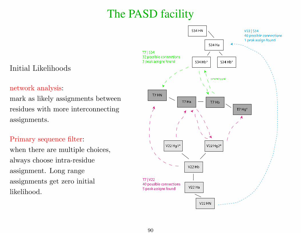
Initial Likelihoods

network analysis:

mark as likely assignments between

residues with more interconnecting

assignments.

Primary sequence filter:

when there are multiple choices,

always choose intra-residue

assignment. Long range

assignments get zero initial

likelihood.

90

The PASD facilityInitial Likelihoods

network analysis: a contact map

25 50 75 100

Residue Number

25

50

75

100

Resi

due N

um

ber

contact map

91

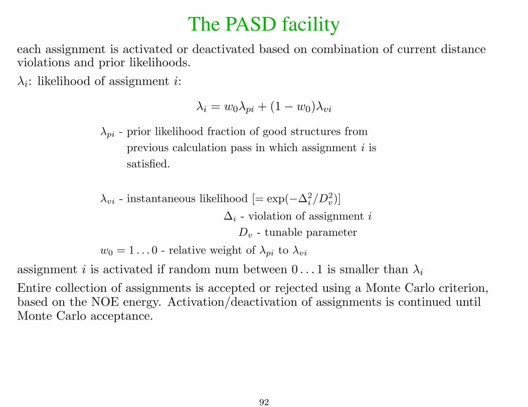
The PASD facilityeach assignment is activated or deactivated based on combination of current distanceviolations and prior likelihoods.

λi: likelihood of assignment i:

λi = w0λpi + (1− w0)λvi

λpi - prior likelihood fraction of good structures from

previous calculation pass in which assignment i is

satisfied.

λvi - instantaneous likelihood [= exp(−∆2i /D

2v)]

∆i - violation of assignment i

Dv - tunable parameter

w0 = 1 . . . 0 - relative weight of λpi to λvi

assignment i is activated if random num between 0 . . . 1 is smaller than λi

Entire collection of assignments is accepted or rejected using a Monte Carlo criterion,based on the NOE energy. Activation/deactivation of assignments is continued untilMonte Carlo acceptance.

92

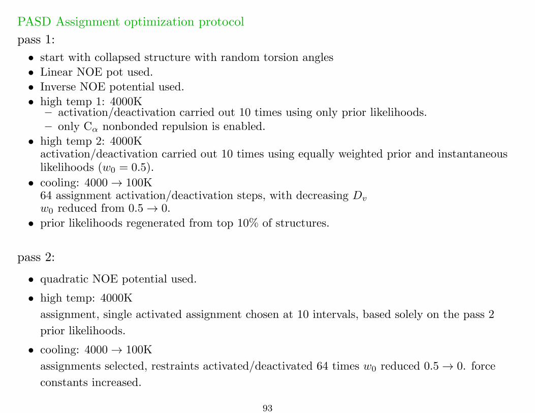
PASD Assignment optimization protocol

pass 1:

• start with collapsed structure with random torsion angles

• Linear NOE pot used.

• Inverse NOE potential used.

• high temp 1: 4000K– activation/deactivation carried out 10 times using only prior likelihoods.– only Cα nonbonded repulsion is enabled.

• high temp 2: 4000Kactivation/deactivation carried out 10 times using equally weighted prior and instantaneouslikelihoods (w0 = 0.5).

• cooling: 4000→ 100K64 assignment activation/deactivation steps, with decreasing Dv

w0 reduced from 0.5→ 0.

• prior likelihoods regenerated from top 10% of structures.

pass 2:

• quadratic NOE potential used.

• high temp: 4000K

assignment, single activated assignment chosen at 10 intervals, based solely on the pass 2

prior likelihoods.

• cooling: 4000→ 100K

assignments selected, restraints activated/deactivated 64 times w0 reduced 0.5→ 0. force

constants increased.

93

The PASD facilityFinal Assignment:

• final likelihoods are computed for each assignment from top 10% of structures.

• incorrect restraint should have all likelihoods near 0• correct restraint should have one assignment with a likelihood near 1.

Results:

• Demonstrated successfully on proteins with over 210 residues.

• method can tolerate about 80% bad NOE data.• failure is clearly indicated by a low value of resulting NOE coverage: the number of

long-range high-likelihood assignments per residue. [ a value > 2 ]

• poor structural precision may mean that the algorithm failed, or that only subregionshave been determined.• regardless, high-likelihood assignments are very likely to be correct.

input formats supported: nmrdraw, nmrstar (including combined version 2.1), pipp,xeasy, Sparky, and NEF.

94

Convenience Scriptspdb2psf - generate a psf from a PDB file.

seq2psf - generate a psf file from primary sequence.

% seq2psf -segname PROT -startresid 300 -protein protG.seqcreates protG.psf with segid PROT starting with residue id 300.

torsionReport - collect and average protein torsion angle values.

% torsionReport -psf=[psf file] [pdb files] >average.info

aveStruct - average structures and report per-atom RMSD to the mean- unregularized.

targetRMSD - report RMSD to a reference structure

pairRMSD.py - report pairwise RMSD

calcTensor - calculate an SVD alignment tensor and report back-calculated RDC valuesgiven one or more structures. Can create plot of observed vs. calculated RDCs.

calcETensor - calculate an ensemble of SVD alignment tensors from an ensemble ofstructures and observed RDC values. The tensors are underdetermined.

calcDaRh - calculate estimates of Da and rhombicity given only RDC values (nostructures) - using a maximum likelihood approach.

calcSARDC - Predict RDCs in steric alignment media from bond vector orientation andmolecular shape, and compare with observed values. Can create plot of observed vs.calculated RDCs.calcSAXS - given a structure, calculate a SAXS or SANS curve, optionally comparingwith experiment. Can also compute optimal excluded solvent parameters (includingboundary layer contribution).

95

Convenience ScriptsmleFit - fit an ensemble of structures based on similarity using a maximum likelihoodalgorithm - no need to specify atom selection.

findClusters - find clusters of similar structures within an ensemble.

domainDecompose - given an ensemble of structures, find regions of structural similarity,using maximum-likelihood fitting.

ens2pdb - convert ensemble of structures into a MODEL-separated pdb for submission.

ramaStrip - plot selected backbone angles in a 2D map showing likely Ramachandranregions for the given residue types.

contactMap - plot a contact map for the specified structures.

scriptMaker - Graphical tool to generate Xplor-NIH scripts (written by Alex Maltsev).

idleXplor - Integrated development environment, including an editor.

convertTalos - Generate Xplor-NIH dihedral restraints from TALOS+ or TALOS-Noutput. These tables are more appropriate than those produced by TALOS itself.

getBest - Helper to print out file names associated to the best structures resulting from aparticular Xplor-NIH calculation. It can also create symbolic links to these files.

96

Where to go for helponline:http://nmr.cit.nih.gov/xplor-nih/ - home pagemailto:xplor-nih@nmr.cit.nih.gov - mailing listhttp://nmr.cit.nih.gov/xplor-nih/faq.html - FAQhttp://nmr.cit.nih.gov/xplor-nih/doc/current/ - current

Documentationhttp://nmr.cit.nih.gov/xplor-nih/doc/current/python/tut.pdf - Tutorialhttp://nmr.cit.nih.gov/xplor-nih/xplor-nih-tutorial.tgz - Hands-on

Examples

subdirectories within the xplor distribution:eginputs - newer complete example scriptstutorial - repository of older XPLOR scriptshelplib - help fileshelplib/faq - frequently asked questions

Python:M. Lutz, “Learning Python, 4th Edition” (O’Reilly, 2009);http://python.org

TCL:J.K. Ousterhout “TCL and the TK Toolkit” (Addison Wesley, 1994);http://www.tcl.tk

Please complain! and suggest!

97