arX

iv:1

508.

0610

3v1

[cs

.NA

] 2

5 A

ug 2

015

Two-level space-time domain decomposition methods for

unsteady inverse problems

Xiaomao Deng ∗ Xiao-chuan Cai† Jun Zou‡

Abstract

As the number of processor cores on supercomputers becomes larger and larger,

algorithms with high degree of parallelism attract more attention. In this work, we

propose a novel space-time coupled algorithm for solving an inverse problem associ-

ated with the time-dependent convection-diffusion equation in three dimensions. We

introduce a mixed finite element/finite difference method and a one-level and a two-

level space-time parallel domain decomposition preconditioner for the Karush-Kuhn-

Tucker (KKT) system induced from reformulating the inverse problem as an output

least-squares optimization problem in the space-time domain. The new full space ap-

proach eliminates the sequential steps of the optimization outer loop and the inner

forward and backward time marching processes, thus achieves high degree of paral-

lelism. Numerical experiments validate that this approach is effective and robust for

recovering unsteady moving sources. We report strong scalability results obtained on

a supercomputer with more than 1,000 processors.

Keywords: Space-time method; Domain decomposition method; Unsteady in-

verse problem; Pollutant source identification; Parallel computing

∗Laboratory for Engineering and Scientific Computing, Shenzhen Institutes of Advanced Technology,

Chinese Academy of Sciences, Shenzhen, Guangdong 518055, P. R. China. (xm.deng@siat.ac.cn)†Department of Computer Science, University of Colorado Boulder, Boulder, CO 80309, USA.

(cai@colorado.edu)‡Department of Mathematics, The Chinese University of Hong Kong, Shatin N.T., Hong Kong, P. R.

China. The work of this author was substantially supported by Hong Kong RGC grants (projects 14306814

and 405513). (zou@math.cuhk.edu.hk)

1

1 Introduction

In this paper, we consider an inverse problem associated with the time-dependent convection-

diffusion equation defined in Ω ∈ R3:

∂C

∂t= ∇ · (a(x)∇C)−∇ · (v(x)C) + f(x, t), 0 < t < T , x ∈ Ω

C(x, t) = p(x, t), x ∈ Γ1

a(x)∂C

∂n= q(x, t), x ∈ Γ2

C(x, 0) = C0(x), x ∈ Ω ,

(1)

where f(x, t) is the source term to be recovered, a(x) and v(x) are the given diffusivity and

convective coefficients. Γ1 and Γ2 are two disjoint parts of the boundary ∂Ω. Dirichlet

and Neumann boundary conditions are imposed respectively on Γ1 and Γ2. When the

observation data C(x, t) is available at certain locations, several classes of inverse problems

associated with the convection-diffusion equation (1) have been investigated, such as the

recovery of the diffusivity coefficient with applications in, for examples, laminar wavy film

flows [20], and flows in porous media [27], the recovery of the source with applications in,

for examples, convective heat transfer problems [25], indoor airborne pollutant tracking

[24], ground water contamination modeling [29, 32, 33, 39], etc.

The main focus of this work is to study the following inverse problem: given the mea-

surement data Cǫ(x, t) of C(x, t) at some locations inside Ω for the period 0 < t < T (ǫ

denotes the noise level), we try to recover the time-varying source locations and intensities,

i.e., the source function f(x, t) in equation (1). In the last decades, several types of numer-

ical methods have been developed for retracing the sources, such as the explicit method

[19], the quasi-reversibility method [33], the statistical method [35] and the Tikhonov

optimization method [4, 12, 18, 36]. Among these methods, the Tikhonov optimization

method is the most popular one, which reformulates the original inverse source problem

into an output least-squares optimization problem with PDE-constraints, and by including

appropriate regularizations it ensures the stability of the resulting optimization problem

[13, 37]. Various techniques are available for solving the induced first-order optimality

system [3, 4, 7, 8, 22].

2

We define the following objective functional with Tikhonov optimization:

J(f) =1

2

∫ T

0

∫

ΩA(x)(C(x, t) − Cǫ(x, t))2 dxdt+Nβ(f) , (2)

where A(x) is the data range indicator function, namely A(x) =∑s

i=1 δ(x − xi), and x1,

x2, · · · , xs are a set of specified locations, where the concentration C(x, t) is measured

and denoted by Cǫ(xi, t). The term Nβ(f) in (2) is called the regularization with respect

to the source. Since f(x, t) depends on both space and time, we propose the following

space-time H1-H1 regularization:

Nβ(f) =β12

∫ T

0

∫

Ω|f(x, t)|2dxdt+

β22

∫ T

0

∫

Ω|∇f |2dxdt . (3)

Here β1 and β2 are two regularization parameters. Other regularizations, such as H1-L2,

may be used, but we will show later by numerical experiments that H1-H1 regularization

may offer better numerical reconstructions.

Traditionally the problem (1)-(3) is solved by a reduced space sequential quadratic

programming(SQP) method [12, 36], which can be described as follows:

Optimization loop (sequential)

Step 1: Solve a forward-in-time state equation

Loop in time (sequential)

- Solve the steady-state equation for this time step (parallel)

End loop

Step 2: Solve a backward-in-time adjoint equation

Loop in time (sequential)

- Solve the steady-state equation for this time step (parallel)

End loop

Step 3: Solve objective equation (parallel)

End loop

3

Parallelization strategies for solving the problem with reduced space SQP methods

include by keeping the sequential steps of the outer loop and applying parallel-in-space

algorithms such as domain decomposition, multigrid methods to the subsystems at each

time step [2]. Reduced space SQP methods for unsteady inverse problems needs repeatedly

solving the state equation, the adjoint equation and the objective equation, thus it divides

the problem into many subproblems, the memory cost is low. However reduced space

SQP methods sometimes are quite time-consuming to achieve convergence. Because of

the sequential steps in the optimization loop and in the forward and backward time-

marching processes, it is less ideal for parallel computers with a large number of processor

cores compared to full space SQP methods. Full space method in [9, 11] has been studied

for steady state problems, for unsteady problems, it needs to eliminate the sequential steps

in the outer loop and solve the full space-time problem as a coupled system. Because of

the much larger size of the system, the full space approach may not be suitable for small

computer systems, but it has fewer sequential steps and thus offers a much higher degree

of parallelism required by large scale supercomputers.

Finding suitable parallelization strategies for the optimization loop and the inner time

loops is an active research area. An unsteady PDE-constrained optimization problem

was solved in [38] for the boundary control of unsteady incompressible flows by solving

a subproblem at each time step. It has the sequential time-marching process and each

subproblem is steady-state. The parareal algorithms were studied in [5, 14, 23], which

involve a coarse (coarse mesh in the time dimension) solver for prediction and a fine (fine

mesh in the time dimension) solver for correction. Parallel implicit time integrator method

(PITA), space-time multigrid, multiple shooting methods can be categorized as improved

versions of the parareal algorithm [16, 17]. The parareal algorithm combined with domain

decomposition method [26] or multigrid method can be powerful. So far, most references

on parareal related studies focus mainly on the stability and convergence [15].

In this paper, we propose a fully implicit, mixed finite element and finite difference

discretization scheme for the continuous KKT system, and a corresponding space-time

overlapping Schwarz preconditioned solver for the unsteady inverse source identification

problem in three dimensions. The method removes all the sequential inner time steps and

achieves full parallelization in both space and time. We study the most general form of

4

the source function, in other words, we reconstruct the time history of the distribution

and intensity profile of the source simultaneously. Furthermore, to resolve the dilemma

that the number of linear iterations of one-level methods increases with the number of

processors, we develop a two-level space-time hybrid Schwarz preconditioner which offers

better performance in terms of the number of iterations and the total compute time.

The rest of the paper is arranged as follows. In Section 2, we describe the mathematical

formulation of the inverse problem and the derivation of the KKT system. We propose, in

Section 3, the main algorithm of the paper, and discuss several technical issues involved

in the fully implicit discretization scheme and the one- and two-level overlapping Schwarz

methods for solving the KKT system. Numerical experiments for the recovery of 3D

sources are given in Section 4, and some concluding remarks are provided in Section 5.

2 Strong formulation of KKT system

We formally write (1) as an operator equation L(C, f) = 0. For G ∈ H1(Ω), the following

Lagrange functional [3, 21] transforms the PDE-constrained optimization problem (2) into

an unconstrained minimization problem. Let

J (C, f,G) =1

2

∫ T

0

∫

ΩA(x)(C(x, t) −Cǫ(x, t))2dxdt

+Nβ(f) + (G,L(C, f)) ,

(4)

where G is a Lagrange multiplier or adjoint variable, and (G,L(C, f)) denotes their in-

ner product. Two approaches are available for solving (4), the optimize-then-discretize

approach and the discretize-then-optimize approach. The first approach derives a contin-

uous optimality condition system and then applies certain discretization scheme, such as a

finite element method to obtain a discrete system ready for computation. The second ap-

proach discretizes the optimization function J , and then the objective functional becomes

a finite dimensional quadratic polynomial. The solution algorithm is then based on the

polynomial system. The two approaches perform the approximation and discretization

at different stages, both have been applied successfully [28], we use the optimize-then-

discretize approach in this paper.

The first-order optimality conditions for (4), i.e., the KKT system, is obtained by

5

taking the variations with respect to G, C and f as

JG(C, f,G)v = 0

JC(C, f,G)w = 0

Jf (C, f,G)g = 0

(5)

for all v,w ∈ L2(0, T ;H1Γ1(Ω)) with zero traces on Γ1 and g ∈ H1(0, T ;H1(Ω)).

Using integration by part, we obtain the strong form of the KKT system:

∂C

∂t−∇ · (a∇C) +∇ · (v(x)C)− f = 0

−∂G

∂t−∇ · (a∇G)− v(x) · ∇G+A(x)C = A(x)Cǫ

G+ β1∂2f

∂t2+ β2∆f = 0 .

(6)

To derive the boundary, initial and terminal conditions for each variable of the equations,

we make use of the property that (5) holds for arbitrary directional functions v,w and

g. For the state equation (i.e. the first one of (5) or (6)) it is obvious to maintain the

same conditions given by (1). For the adjoint equation (the second one of (5) or (6)), by

multiplying the test function w ∈ L2(0, T ;H1Γ1(Ω)) with w(·, 0) = 0, a(x)∂w

∂n= 0 on Γ2,

we have

JC(C, f,G)w =

∫ T

0

∫

ΩA(x)(C(x, t) − Cǫ(x, t))wdxdt +

∫

ΩG(x, T )w(x, T )dx

−

∫ T

0

∫

Ω

(

∂G

∂t+∇ · (a(x)∇G) + v(x) · ∇G

)

wdxdt

−

∫ T

0

∫

Γ1

(

a(x)∂w

∂n

)

GdΓdt

+

∫ T

0

∫

Γ2

(

a(x)∂G

∂n+ v(x) · n

)

wdΓdt .

By the arbitrariness of w, the boundary and terminal conditions for G are derived:

G(x, t) = 0, x ∈ Γ1, t ∈ [0, T ]

a(x)∂G

∂n+ v(x) · n = 0, x ∈ Γ2, t ∈ [0, T ]

G(x, T ) = 0, x ∈ Ω .

6

Similarly for the third equation of (5) or (6), we can deduce

Jf (C, f,G)g = −

∫ T

0

∫

ΩGgdxdt +

∫ T

0

∫

Ω(f g +∇f · ∇g)dxdt

= −

∫ T

0

∫

ΩGgdxdt + (f g)|t=0,T −

∫ T

0

∫

Ωfg

+

∫ T

0

∫

∂Ω

∂f

∂ngdΓdt−

∫ T

0

∫

Ω∆fgdxdt

= −

∫ T

0

∫

Ω(G+ f +∆f)gdxdt+ (fg)|t=0,T +

∫ T

0

∫

∂Ω

∂f

∂ngdΓdt .

Using the arbitrariness of g, we derive the boundary, initial and terminal conditions for f :

∂f

∂t= 0 for t = 0, T, x ∈ Ω ;

∂f

∂n= 0 for x ∈ ∂Ω, t ∈ [0, T ] . (7)

3 A fully implicit and fully coupled method

In this section, we first introduce a mixed finite element and finite difference method for

the discretization of the continuous KKT system derived in the previous section, then we

briefly mention the algebraic structure of the discrete system of equations. In the second

part of the section, we introduce the one- and two-level space-time Schwarz preconditioners

that are the most important components for the success of the overall algorithm.

3.1 Fully-implicit space-time discretization

In this subsection, we introduce a fully-implicit finite element/finite difference scheme to

discretize (6). To discretize the state and the adjoint equations, we use a second-order

Crank-Nicolson finite difference scheme in time and a piece-wise linear continuous finite

element method in space. Consider a regular triangulation T h of domain Ω, and a time

partition P τ of the interval [0, T ]: 0 = t0 < t1 < · · · < tM = T, with tn = nτ, τ = T/M .

Let V h be the piecewise linear continuous finite element space on T h, and V h be the

subspace of V h with zero trace on Γ1. We introduce the difference quotient and the

averaging of a function ψ(x, t) as

∂τψn(x) =

ψn(x)− ψn−1(x)

τ, ψn(x) =

1

τ

∫ tn

tn−1

ψ(x, t)dt ,

with ψn(x) := ψ(x, tn). Let πh be the finite element interpolation associated with the

space V h, then we obtain the discretizations for the state and adjoint equations by finding

7

the sequence of approximations Cnh , G

nh ∈ V h, such that C0

h = πhC0, GMh = 0, and

Cnh (x) = πhp(x, t

n), Gnh(x) = 0 for x ∈ Γ1, and satisfying

(∂τCnh , vh) + (a∇Cn

h ,∇vh) + (∇ · (vCnh ), vh) = (fnh , vh) + 〈qn, vh〉Γ2

, ∀ vh ∈ V h

−(∂τGnh, wh) + (a∇Gn

h,∇wh) + (∇ · (vwh), Gnh)

= −(A(x)(Cnh (x, t)− Cǫ,n(x, t)), wh), ∀wh ∈ V h .

(8)

Unlike the approximations of the forward and adjoint equations in (8), we shall ap-

proximate the source function f differently. We know that the source function satisfies an

elliptic equation (see the third equation in (6)) in the space-time domain Ω× (0, T ). So we

shall apply T h×P τ to generate a partition of the space-time domain Ω× (0, T ), and then

apply the piecewise linear finite element method in both space (three dimensions) and

time (one dimension), denoted by W τh , to approximate the source function f . Then the

equation for f ∈ W τh can be discretized as follows: Find the sequence of fnh for n = 0, 1,

· · · , M such that

− (Gnh, g

τh) + β1(∂τf

nh , ∂τg

τh) + β2(∇f

nh ,∇g

τh) = 0, ∀ gτh ∈W τ

h . (9)

The coupled system (8)-(9) is the so-called fully discretized KKT system. In the Appendix,

we provide some details of the discrete structure of this KKT system.

3.2 One- and two-level space-time Schwarz preconditioning

Usually, the unknowns of the KKT system (8)-(9) are ordered physical variable by physical

variable, namely in the form

U = (C0, C1, · · · , CM , G0, G1, · · · , GM , f0, f1, · · · , fM)T .

Such ordering are used extensively in SQP methods [12]. In our all-at-once method, the

unknowns C,G and f are ordered mesh point by mesh point and time step by time step,

and all unknowns associated with a point stay together as a block. At each mesh point xj,

j = 1, · · · , N , and time step tn, n = 0, · · · , M , the unknowns are arranged in the order

of Cnj , G

nj , f

nj . Such ordering avoids zero values on the main diagonal of the matrix and

has better cache performance for point-block LU (or ILU) factorization based subdomain

8

solvers. More precisely, we define the solution vector

U = (C01 , G

01, f

01 , · · · , C

0N , G

0N , f

0N , C

11 , G

11, f

11 , · · · , C

1N , G

1N , f

1N , · · · , C

M1 , GM

1 , fM1 ,

· · · , CMN , GM

N , fMN )T .

then the linear system (8)-(9) is rewritten as

FhU = b , (10)

where Fh is a sparse block matrix of size (M +1)(3N) by (M +1)(3N) with the following

block structure:

Fh =

S00 S01 0 · · · 0

S10 S11 S12 · · · 0

0. . .

. . .. . . 0

0 · · · SM−1,M−2 SM−1,M−1 SM−1,M

0 · · · 0 SM,M−1 SM,M

,

where the block matrices Sij for 0 ≤ i, j ≤M are of size 3N×3N and most of its elements

are zero matrices except the ones in the tridiagonal stripes Si,i−1, Si,i, Si,i+1. It is

noted that if we denote the submatrices for C,G and f of size N × N respectively by

SCij , S

Gij , S

fij in each block Sij, the sparsity of the matrices are inconsistent, namely, Sf

ij

is the densest and SGij is the sparest. This is due to the discretization scheme we have

used. The system (10) is large-scale and ill-conditioned, therefore is difficult to solve

because the space-time coupled system is denser than the decoupled system, especially for

three dimensional problems. We shall design the preconditioner by extending the classical

spatial Schwarz preconditioner to include both spaial and temporal variables. Such an

approach eliminates all sequential steps and the unknowns at all time steps are solved

simultaneously. We use a right-preconditioned Krylov subspace method to solve (10),

FhM−1U ′ = b ,

where M−1 is a space-time Schwarz preconditioner and U =M−1U ′.

Denoting the space-time domain by Θ = Ω × (0, T ), an overlapping decomposition of

Θ is defined as follows: we divide Ω into Ns subdomains, Ω1,Ω2, · · · , ΩNs, then partition

9

Figure 1: Left: a sample overlapping decomposition in space-time domain Θ on a fine

mesh. Right: the same decomposition on the coarse mesh.

the time interval [0, T ] into Nt subintervals using the partition: 0 < T1 < T2 < · · · <

TNt. By coupling all the space subdomains and time subintervals, a decomposition of

Θ is Θ = ∪Ns

i=1(∪Nt

j=1Θij), where Θij = Ωi × (Tj−1, Tj). For convenience, the number of

subdomains, i.e. NsNt, is equal to the number of processors. These subdomains Θij are

then extended to Θ′ij to overlap each other. The boundary of each subdomain is extended

by an integral number of mesh cells in each dimension, and we trim the cells outside of

Θ. The corresponding overlapping decomposition of Θ is Θ = ∪Ns

i=1(∪Nt

j=1Θ′ij). See the left

figure of Figure 1 for the overlapping extension.

The matrix on each subdomain Θ′ij = Ω′

i × (T ′j−1, T

′j), i = 1, 2, · · · , Ns, j = 1, 2, · · · ,

Nt is the discretized version of the following system of PDEs

∂C

∂t= ∇ · (a(x)∇C)−∇ · (v(x)C) + f(x, t) , (x, t) ∈ Θ′

ij

∂G

∂t= −∇ · (a(x)∇G) − v(x) · ∇G

+A(x)(C(x, t) − Cε(x, t)) , (x, t) ∈ Θ′ij

β1∂2f

∂t2+ β2∆f +G = 0 , (x, t) ∈ Θ′

ij

(11)

with the following boundary conditions

C(x, t) = 0, G(x, t) = 0, f(x, t) = 0 , x ∈ ∂Ω′i , t ∈ [T ′

j−1, T′j ] (12)

10

along with the initial and terminal time boundary conditions

C(x, T ′j−1) = 0, G(x, T ′

j−1) = 0, f(x, T ′j−1) = 0 , x ∈ ∂Ω′

i

C(x, T ′j) = 0, G(x, T ′

j) = 0, f(x, T ′j) = 0 , x ∈ ∂Ω′

i .

(13)

One may notice from (13) that the homogenous Dirichlet boundary conditions are

applied in each time interval (T ′j−1, T

′j), so the solution of each subdomain problem is

not really physical. This is one of the major differences between the space-time Schwarz

method and the parareal algorithm [23]. The time boundary condition for each subproblem

of the parareal algorithm is obtained by an interpolation of the coarse solution, and if the

coarse mesh is fine enough, the solution of the subdomain problem is physical. As a result,

the parareal algorithms can be used as a solver, but our space-time Schwarz method

can only be used as a preconditioner. Surprisingly, as we shall see from our numerical

experiments in Section 4, the Schwarz method is an excellent preconditioner even though

the time boundary conditions violate the physics.

We solve the subdomain problems the same as for the global problem (10), no time-

marching is performed in our new algorithm, and all unknowns affiliated with each sub-

domain are solved simultaneously. Let Mij be the matrix generated in the same way as

the global matrix Fh in (10) but for the subproblem (11)-(13), and M−1ij be an exact or

approximate inverse of Mij . Denoting the restriction matrix from Θ to the subdomain Θ′ij

by Rδij, with overlapping size δ, the space-time restricted Schwarz preconditioner [10] can

be now formulated as

M−1one−level =

Nt∑

j=1

Ns∑

i=1

(Rδij)

T M−1ij R

0ij .

As it is well known, any one-level domain decomposition methods are not scalable with

the increasing number of subdomains or processors. Instead one should have multilevel

methods in order to observe possible scalable effects [1, 34]. We now propose a two-level

space-time additive Schwarz preconditioner. To do so, we partition Ω with a fine mesh

Ωh and a coarse mesh Ωc. For the time interval, we have a fine partition P τ and a coarse

partition P τc with τ < τc. We will adopt a nested mesh, i.e., the nodal points of the coarse

mesh Ωc ×P τc are a subset of the nodal points of the fine mesh Ωh ×P τ . In practice, the

size of the coarse mesh should be adjusted properly to obtain the best performance. On

11

the fine level, we simply apply the previously defined one-level space-time additive Schwarz

preconditioner; and to efficiently solve the coarse problem, a parallel coarse preconditioner

is also necessary. Here we use the overlapping space-time additive Schwarz preconditioner

and for simplicity divide Ωc×P τc into the same number of subdomains as on the fine level,

using the non-overlapping decomposition Θ = ∪Ns

i=1(∪Nt

j=1Θij). When the subdomains are

extended to overlapping ones, the overlapping size is not necessarily the same as that

on the fine mesh. See the right figure of Figure 1 for a coarse version of the space-time

decomposition. We denote the preconditioner for the coarse level byM−1c , which is defined

by

M−1c =

Nt∑

j=1

Ns∑

i=1

(Rδcij,c)

T M−1ij,cR

0ij,c ,

where δc is the overlapping size on the coarse mesh. Here the matrix M−1ij,c is an approxi-

mate inverse of Mij,c which is obtained by a discretization of (11)-(13) on the coarse mesh

on Θ′ij.

To combine the coarse preconditioner with the fine mesh preconditioner, we need a

restriction operator Ich from the fine to coarse mesh and an interpolation operator Ihc

from the coarse to fine mesh. For our currently used nested structured mesh and linear

finite elements, Ihc is easily obtained using a linear interpolation on the coarse mesh and

Ich = (Ihc )T . We note that when the coarse and fine meshes are nested, instead of using

Ich = (Ihc )T , we may take Ich to be a simple restriction, e.g., the identity one which assigns

the values on the coarse mesh using the same values on the fine mesh. In general, the coarse

preconditioner and the fine preconditioner can be combined additively or multiplicatively.

According to our experiments, the following multiplicative version works well:

y = Ihc F−1c Ichx

M−1two−levelx = y +M−1

one−level(x− Fhy) ,

(14)

where F−1c corresponds to the GMRES solver right-preconditioned by M−1

c on the coarse

level, and Fh is the discrete KKT system (10) on the fine level.

12

4 Numerical experiments

In this section we present some numerical experiments to study the parallel performance

and robustness of the newly developed algorithms. When using the one-level precondi-

tioner, we use a restarted GMRES method (restarts at 50) to solve the preconditioned

system; when using the two-level preconditioner, we use the restarted flexible GMRES

(fGMRES) method [30] (restarts at 30), considering the fact that the overall precondi-

tioner changes from iteration to iteration because of the iterative coarse solver. Although

fGMRES needs more memory than GMRES, we have observed its number of iterations

can be significantly reduced. The relative convergence tolerance of both GMRES and

fGMRES is set to be 10−6. The initial guesses for both GMRES and fGMRES method

are zero. The size of the overlap between two neighbouring subdomains, denoted by iovlp,

is set to be 1 unless otherwise specified. The subsystem on each subdomain is solved by

an incomplete LU factorization ILU(k), with k being its fill-in level, and k = 0 if not

specified. The algorithms are implemented based on the Portable, Extensible Toolkit for

Scientific computation (PETSc) [6] using run on a Dawning TC3600 blade server system

at the National Supercomputing Center in Shenzhen, China with a 1.271 PFlops/s peak

performance.

In our computations, the settings for the model system (1) are taken as follows.

The computational domain, the terminal time and the initial condition are taken to

be Ω = (−2, 2)3, T = 1 and C(·, 0) = 0 respectively. Let L = S = H = 2, then

the homogeneous Dirichlet and Neumann conditions in (1) are respectively imposed on

Γ1 = x = (x1, x2, x3); |x1| = L or |x2| = S and Γ2 = x = (x1, x2, x3); |x3| = H.

Furthermore, the diffusivity and convective coefficients are set to be a(x) = 1.0 and

v(x) = (1.0, 1.0, 1.0)T .

In order to generate the observation data, we solve the forward convection-diffusion

equation (1) on a very fine mesh with a small time step size, and the resulting approximate

solution C(x, t) is used as the noise-free observation data. Then a random noise is added

in the following form at the locations where the measurements are taken:

Cǫ(xi, t) = C(xi, t) + ǫ r C(xi, t), i = 1, · · · , s .

Here r is a random function with the standard Gaussian distribution, and ǫ is the noise

13

−2

−1

0

1

2

−2

−1

0

1

2−2

−1.5

−1

−0.5

0

0.5

1

1.5

2

xy

t

t=0

t=0

Figure 2: The traces of two moving sources.

level. In our numerical experiments, ǫ = 1% if not specified otherwise.

The numerical tests are designed to investigate the reconstruction effects with different

types of three-dimensional sources by the proposed one- or two-level space-time Schwarz

method, as well as the robustness of the algorithm with respect to different noise level,

different regularizations and different amount of measurement data. In addition, parallel

efficiency of the proposed algorithms is also studied.

4.1 Reconstruction of 3D sources

We devote this subsection to test the numerical reconstruction of three representative 3D

sources by the proposed one-level space-time method, with np = 256 processors. Each of

the three examples are constructed with its own special difficulty.

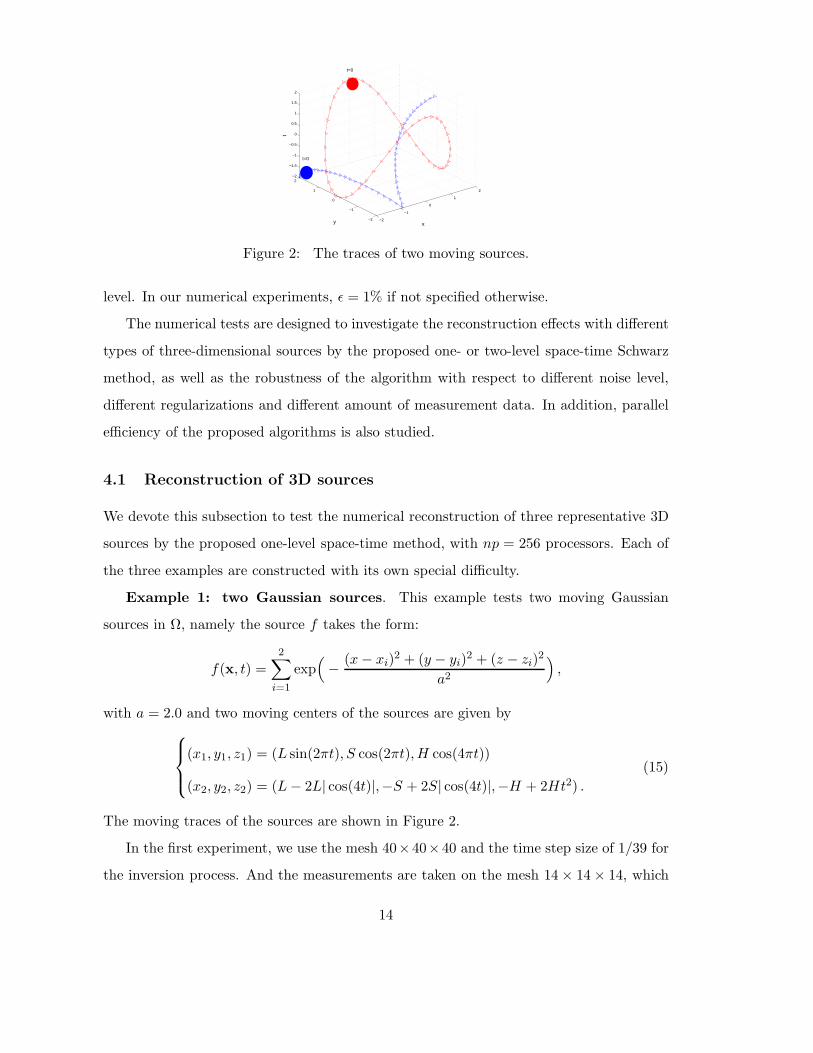
Example 1: two Gaussian sources. This example tests two moving Gaussian

sources in Ω, namely the source f takes the form:

f(x, t) =2

∑

i=1

exp(

−(x− xi)

2 + (y − yi)2 + (z − zi)

2

a2

)

,

with a = 2.0 and two moving centers of the sources are given by

(x1, y1, z1) = (L sin(2πt), S cos(2πt),H cos(4πt))

(x2, y2, z2) = (L− 2L| cos(4t)|,−S + 2S| cos(4t)|,−H + 2Ht2) .

(15)

The moving traces of the sources are shown in Figure 2.

In the first experiment, we use the mesh 40×40×40 and the time step size of 1/39 for

the inversion process. And the measurements are taken on the mesh 14× 14× 14, which

14

Figure 3: Example 1: the source reconstructions at three moments t =

10/39, 20/39, 30/39 with measurements collected at the mesh 14× 14× 14 (bottom), com-

parable with the exact source distribution (top).

is uniformly located in Ω. The regularization parameters are set to be β1 = 3.6 × 10−5

and β2 = 3.6 × 10−3. In Figure 3, the numerically reconstructed sources are compared

with the exact one at three moments t = 10/39, 20/39, 30/39. We can see that the source

locations and intensities are quite close to the true values at three chosen moments. Then

we increase the noise level to ǫ = 5% and ǫ = 10%, still with the same set of parameters.

The reconstruction results are shown in Figure 4. We can observe that the reconstructed

profiles deteriorate and become oscillatory as the noise level increases. This is naturally

expected since the ill-posedness of the inverse source problem increases with the noise

level.

Example 2: Four constant sources. Appropriate choices of regularizations are

important for the inversion process. In the previous example we have used a H1-H1

Tikhonov regularization in both space and time. In this example, we intend to compare

15

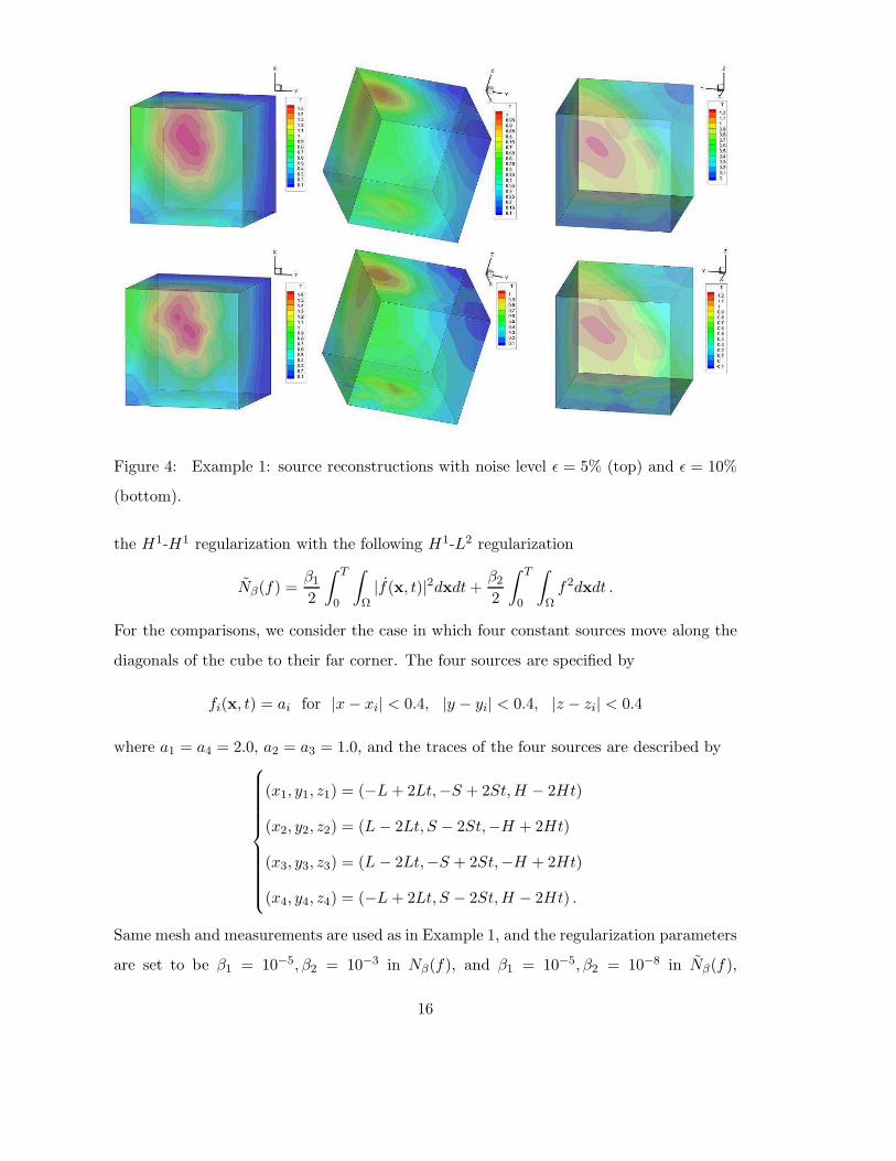
Figure 4: Example 1: source reconstructions with noise level ǫ = 5% (top) and ǫ = 10%

(bottom).

the H1-H1 regularization with the following H1-L2 regularization

Nβ(f) =β12

∫ T

0

∫

Ω|f(x, t)|2dxdt+

β22

∫ T

0

∫

Ωf2dxdt .

For the comparisons, we consider the case in which four constant sources move along the

diagonals of the cube to their far corner. The four sources are specified by

fi(x, t) = ai for |x− xi| < 0.4, |y − yi| < 0.4, |z − zi| < 0.4

where a1 = a4 = 2.0, a2 = a3 = 1.0, and the traces of the four sources are described by

(x1, y1, z1) = (−L+ 2Lt,−S + 2St,H − 2Ht)

(x2, y2, z2) = (L− 2Lt, S − 2St,−H + 2Ht)

(x3, y3, z3) = (L− 2Lt,−S + 2St,−H + 2Ht)

(x4, y4, z4) = (−L+ 2Lt, S − 2St,H − 2Ht) .

Same mesh and measurements are used as in Example 1, and the regularization parameters

are set to be β1 = 10−5, β2 = 10−3 in Nβ(f), and β1 = 10−5, β2 = 10−8 in Nβ(f),

16

Figure 5: Example 2: the source reconstructions with H1-H1 regularization (mid) and

H1-L2 regularization (bottom), compared with the exact solution (top).

respectively. The reconstruction results are compared with the true solution at three

moments t = 10/39, 20/39, 30/39, and two slices at x = 0.95 and x = −0.95. It is

observed from Figure 5 that the resolution of the source profile is much better with the

H1-H1 regularization Nβ(f) than with the H1-L2 regularization Nβ(f), and the latter

presents a reconstruction process that is much less stable and much more oscillatory.

Example 3: Eight moving sources. This last example presents a very challenging

case that eight Gaussian sources are initially located at the corners of the physical cubic

domain, then move inside the cube following their own traces given below. The Gaussian

17

sources are described by

f(x, t) =

8∑

i=1

aie−(x−xi)2+(y−yi)2+(z−zi)2 ,

where the coefficients ai and the source traces are represented by

a1 = a2 =a3 = a4 = 4.0; a5 = a6 = a7 = a8 = 6.0,

(x1, y1, z1) = (−L+ 2L(1− t),−S + 2S(1− t),−H + 2H(1 − t))

(x2, y2, z2) = (−L+ 2Lt,−S + 2St,−H + 2Ht)

(x3, y3, z3) =(

−L+ 2L cos(πt)2(1− t),−S + 2S sin(πt)2t,−H + 2H cos(πt)2(1− t))

(x4, y4, z4) =(

−L+ 2L cos(πt)2(1− t),−S + 2S cos(πt)2(1− t),−H + 2H sin(πt)2t))

(x5, y5, z5) =(

−L+ 2L cos(2πt)2 cos (π/2t) ,−S + 2S sin(π t)2 sin (π/2t) ,

−H + 2H sin(πt)2 sin (π/2t))

(x6, y6, z6) =(

−L+ 2L sin(πt)2 sin (π/2t) ,−S + 2S cos(2π t)2 cos (π/2t) ,

−H + 2H sin(πt)2 sin (π/2t))

(x7, y7, z7) =(

−L+ 2L sin(πt)2 sin (π/2t) ,−S + 2S sin(π t)2 sin (π/2t) ,

−H + 2H cos(2πt)2 cos (π/2t))

(x8, y8, z8) =(

−L+ 2L sin(πt)2 sin (π/2t) ,−S + 2S cos(2π t)2 cos (π/2t) ,

−H + 2H cos(2πt)2 cos (π/2t))

.

We shall use the mesh 64 × 64 × 64 and the time step size 1/47, with two regularization

parameters β1 = 3.6×10−5 and β2 = 3.6×10−1. We compare the results recovered by two

sets of measurements, collected at two meshes 21×21×21 and 9×9×9 respectively, which

are both uniformly distributed in Ω, with the exact solution shown in Figure 6 (top), at

three time moments t = 0.0, 10/47, 1.0. Clearly better reconstructions are observed for

the case with more measurements collected at the finer mesh 21 × 21 × 21, though the

coarser mesh 9× 9× 9 is good enough for locating the sources, only with their recovered

source intensities smaller than the true values.

4.2 Performance in parallel efficiency

In the previous subsection, we have shown with 3 representative examples that the pro-

posed algorithm can successfully recover the intensities and distributions of unsteady

18

Figure 6: Example 3: the source reconstructions with measurements collected at the

mesh 21× 21× 21 (mid) and 9× 9× 9 (bottom), compared with the exact solution (top)

19

Table 1: Effects of ILU fill-in levels on the two-level method for Example 1 (columns 2-3),

Example 2 (columns 4-5), and Example 3 (columns 6-7).

ILU(k) Its Time (sec) Its Time (sec) Its Time (sec)

0 47 10.498 55 12.448 81 17.238

1 28 33.633 36 47.766 60 49.622

2 18 230.552 23 232.914 48 257.798

3 15 1121.469 20 1132.841 45 1165.203

sources and is robust with respect to the noise in the data, the choice of Tikhonov regular-

izations and the number of measurements. These numerical simulations are all computed

using the proposed one-level space-time method with np = 256 processors. In this section,

we focus on our proposed two-level space-time method and study its parallel efficiency

with respect to the number of ILU fill-in levels, namely the number k in ILU(k), and the

overlap size iovlp. We also compare the number of iterations and the total compute time

of the one-level and two-level methods with increasing degrees of freedoms (DOFs) and

the number of processors.

First we will test how the number of fGMRES iterations and the total compute time

of the two-level method change with different ILU fill-in levels. We use the coarse mesh

21 × 21 × 21 with the time step 1/20, and the fine mesh 41 × 41× 41 with the time step

1/40 for Example 1, 2, and 3, and the overlap size iovlp = 1. We see that the total number

of degrees of freedom on the fine mesh is 16 times of the one on the coarse mesh. Table

1 shows the comparison with np = 256 processors. Column 2-3, 4-5 and 6-7 present the

results for Example 1, 2 and 3 respectively. It is observed that as the fill-in level increases

the number of fGMRES iterations decreases, but the total compute time increases. When

the fill-in level increases to 3, the compute time increases significantly and the number of

iterations only reduces by 3 times. This suggests a suitable fill-in level to be ilulevel = 0

or 1.

Next we look at the impact of the overlap size. We still use the same fine and coarse

meshes for all examples, and ILU(0) for the solver for each subdomain problem on both

the coarse and fine meshes. The overlap size on the coarse mesh is set to be 1. We test

20

Table 2: Effects of the overlap size on the two-level method for Example 1 (columns 2-3),

Example 2 (columns 4-5), and Example 3 (columns 6-7).

iovlp Its Time (sec) Its Time (sec) Its Time (sec)

1 47 10.498 55 12.448 81 17.238

2 39 13.071 51 23.663 69 27.952

4 37 27.423 49 45.225 68 47.032

different overlap sizes on the fine level, and the results are given in Table 2. It is observed

that when the overlap size increases from 1 to 2 and then to 4, the number of fGMRES

iterations decreases slowly and the total compute time increases. So we shall mostly use

iovlp = 1 in our subsequent computations.

Lastly we compare the performance of the one-level and two-level space-time Schwarz

preconditioners in Tables 3 and 4. On the coarse level, a restarted GMRES is used, with the

one-level space-time Schwarz preconditioner. ILU(0) is used as the local preconditioner

on each subdomain and the coarse overlap size is set to be 1. A tighter convergence

tolerance on the coarse mesh can reduce the number of outer fGMRES iterations, but

often increases the total compute time. In the following numerical examples, we set the

tolerance to be 10−1 and the maximum number of GMRES iterations to 4 on the coarse

mesh. Moreover, the mesh size of the coarse mesh is also an important factor for the

performance. If the mesh is too coarse, both the number of outer iterations and the total

compute time increase; on the other hand, if the mesh is not coarse enough, too much time

is spent for the coarse solver, the number of outer iterations may decrease significantly,

but the compute time may increase.

In the following experiments for Example 1, 2 and 3, we use three sets of fine meshes,

33×33×33, 49×49×49 and 67×67×67, and the corresponding time steps are 1/32, 1/48

and 1/66 respectively, while the coarse meshes are chosen to be 17× 17× 17, 17× 17× 17

and 23 × 23 × 23, with the corresponding time steps being 1/16, 1/48 and 1/66. So the

DOFs on the fine meshes are 16, 27 and 27 times of the ones on the coarse meshes for

Example 1, 2 and 3 respectively. We use np = 64, 128 and 512 processors for the three sets

of meshes respectively and compare their performance with the one-level method in Table

21

3. Savings in terms of the number of iterations and the total compute time are obtained

for the two-level method with all three sets of meshes. As we observe that the number of

iterations of the two-level method is mostly reduced by at least 4 times compared to the

one for the one-level method, but the compute time is usually reduced by 2 to 4 times.

Next we fix the space mesh to be 49×49×49 and the time step to be 1/48, resulting in

a very large-scale discrete system with 17,294,403 DOFs. For the two-level method, we set

the coarse mesh to be 17× 17× 17 with the time step 1/48, which implies that the DOFs

on the fine mesh is about 27 times of the ones on the coarse mesh. Then the problem is

solved with np = 128, 256, 512, and 1024 processors respectively. The performance results

of the one-level and two-level methods are presented in Table 4. We observe that when

the number of sources is small, both the one-level and two-level methods are scalable

with up to 512 processors, but the two-level method takes much less compute time. The

strong scalability deteriorates when the number of processors is too large for the size of

the problems. As the number of sources increases, the scalability becomes slightly worse

for both one-level and two-level methods, even though the two-level method is still faster

in terms of the total compute time.

5 Concluding remarks

In this work we have proposed and studied a new fully implicit, space-time coupled, mixed

finite element and finite difference discretization method, and a parallel one- and two-

level domain decomposition solver for the three-dimensional unsteady inverse convection-

diffusion problem. With a suitable number of measurements, this all-at-once approach

provides acceptable reconstruction of the physical sources in space and time simultane-

ously. The classical overlapping Schwarz preconditioner is extended successfully to the

coupled space-time problem with a homogenous Dirichlet boundary condition applied on

both the spatial and temporal part of the space-time subdomain boundaries. The one-

level method is easier to implement, but the two-level hybrid space-time Schwarz method

performs much better in terms of the number of iterations and the total compute time.

Good scalability results were obtained for problems with more than 17 millions degrees of

freedom on a supercomputer with more than 1,000 processors. The approach is promising

22

Table 3: Comparisons between the one-level and two-level space-time preconditioners for

Examples 1-3 with different meshes.

Ex1

np Mesh M level Its Time (sec)

64 33× 33× 33 33 1 175 53.635

2 57 20.653

128 49× 49× 49 49 1 346 200.664

2 83 47.812

512 67× 67× 67 67 1 491 675.985

2 105 212.72

Ex2

np Mesh M level Its Time (sec)

64 33× 33× 33 33 1 228 72.338

2 77 20.246

128 49× 49× 49 49 1 365 214.058

2 85 47.078

512 67× 67× 67 67 1 599 841.652

2 121 216.92

Ex3

np Mesh M level Its Time (sec)

64 33× 33× 33 33 1 297 82.834

2 76 21.738

128 49× 49× 49 49 1 405 238.712

2 93 57.244

512 67× 67× 67 67 1 716 872.766

2 137 263.222

23

Table 4: Comparisons between the one-level and two-level space-time preconditioners for

Examples 1-3 with different number of processors.

Ex1 Ex2 Ex3

np level Its Time (sec) Its Time (sec) Its Time (sec)

128 1 346 200.664 365 214.815 405 238.712

2 83 47.812 85 47.072 93 57.244

256 1 343 127.035 363 152.334 408 145.213

2 82 24.744 87 26.424 90 36.307

512 1 343 69.482 363 95.707 400 101.343

2 82 16.461 101 19.453 100 18.611

1024 1 351 41.821 393 58.785 433 59.534

2 85 10.132 100 11.352 104 15.815

to more general unsteady inverse problems in large-scale applications.

References

[1] Aitbayev, R., Cai, X.-C., Paraschivoiu, M.: Parallel two-level methods for three-

dimensional transonic compressible flow simulations on unstructured meshes. Proceed-

ings of Parallel CFD’99 (1999)

[2] Akcelik, V., Biros, G., Draganescu, A., Ghattas, O., Hill, J., Waanders, B.: Dynamic

data-driven inversion for terascale simulations: Real-time identification of airborne con-

taminants. Proceedings of Supercomputing, Seattle, WA (2005)

[3] Akcelik, V., Biros, G., Ghattas, O., Long, K. R., Waanders, B.: A variational finite

element method for source inversion for convective-diffusive transport. Finite Elem.

Anal. Des. 39, 683-705 (2003)

[4] Atmadja, J., Bagtzoglou, A. C.: State of the art report on mathematical methods for

groundwater pollution source identification. Environ. Forensics 2, 205-214 (2001)

24

[5] Baflico, L., Bernard, S., Maday, Y., Turinici, G., Zerah, G.: Parallel-in-time molecular-

dynamics simulations. Phys. Rev. E 66, 2-5 (2002)

[6] Balay, S., Buschelman, K., Eijkhout, V., Gropp, W. D., Kaushik, D., Knepley, M. G.,

McInnes, L. C., Smith, B. F., Zhang, H.: PETSc Users Manual. Technical Report,

Argonne National Laboratory (2014)

[7] Battermann, A.: Preconditioners for Karush-Kuhn-Tucker Systems Arising in Optimal

Control. Master Thesis, Virginia Polytechnic Institute and State University, Blacksburg,

Virginia (1996)

[8] Biros, G., Ghattas, O.: Parallel preconditioners for KKT systems arising in optimal

control of viscous incompressible flows. Proceedings of Parallel CFD’99, Williamsburg,

Virginia, USA (1999)

[9] Cai, X.-C., Liu, S., Zou, J.: Parallel overlapping domain decomposition methods for

coupled inverse elliptic problems. Comm. App. Math. Com. Sc. 4, 1-26 (2009)

[10] Cai, X.-C., Sarkis, M.: A restricted additive Schwarz preconditioner for general sparse

linear systems. SIAM J. Sci. Comput. 21, 792-797 (1999).

[11] Chen, R. L., Cai, X.-C.: Parallel one-shot Lagrange-Newton-Krylov-Schwarz algo-

rithms for shape optimization of steady incompressible flows. SIAM J. Sci. Comput.

34, 584-605 (2012)

[12] Deng, X. M., Zhao, Y. B., Zou, J.: On linear finite elements for simultaneously

recovering source location and intensity. Int. J. Numer. Anal. Mod. 10, 588-602 (2013)

[13] Engl, H. W., Hanke, M., Neubauer, A.: Regularization of Inverse Problems. Kluwer

Academic Publishers, Netherland (1998)

[14] Farhat, C., Chandesris, M.: Time-decomposed parallel time-integrators: theory and

feasibility studies for fluid, structure, and fluid-structure applications. Int. J. Numer.

Meth. Eng. 58, 1397-1434 (2003)

25

[15] Gander, M. J., Hairer, E.: Nonlinear convergence analysis for the parareal algorithm.

Proceedings of the 17th International Conference on Domain Decomposition Methods

60, 45-56 (2008)

[16] Gander, M. J., Petcu, M.: Analysis of a Krylov subspace enhanced parareal algorithm

for linear problems. Paris- Sud Working Group on Modeling and Scientific Computing

2007- 2008 (E. Cances et al., eds.), ESAIM Proc. EDP Sci., LesUlis 25, 114-129 (2008)

[17] Gander, M. J., Vandewalle, S.: Analysis of the parareal time-parallel time-integration

method. SIAM J. Sci. Comput. 29, 556-578 (2007)

[18] Gorelick, S., Evans, B., Remson, I.: Identifying sources of groundwater pollution: an

optimization approach. Water Resour. Res. 19, 779-790 (1983)

[19] Hamdi, A.: The recovery of a time-dependent point source in a linear transport

equation: application to surface water pollution. Inverse Probl., 24, 1-18 (2009)

[20] Karalashvili, M., Groβ, S., Marquardt, W., Mhamdi, A., Reusken, A.: Identification

of transport coefficient models in convection-diffusion equations. SIAM J. Sci. Comput.

33, 303-327 (2011)

[21] Keung, Y. L., Zou, J.: Numerical identifications of parameters in parabolic systems.

Inverse Probl. 14, 83-100 (1998)

[22] Kuhn, H. W., Tucker, A. W.: Nonlinear programming. Proceedings of 2nd Berkeley

Symposium, Berkeley: University of California Press, 481-492 (1951)

[23] Lions, J.-L., Maday, Y., Turinici, G.: A parareal in time discretization of PDE’s.

ComptesRendus de l’Academie des Sciences Series I Mathematics 332, 661-668 (2001)

[24] Liu, X., Zhai, Z.: Inverse modeling methods for indoor airborne pollutant tracking

literature review and fundamentals. Indoor Air 17, 419-438 (2007)

[25] Zhang, J., Delichatsios, M. A.: Determination of the convective heat transfer coeffi-

cient in three-dimensional inverse heat conduction problems. Fire Safety J. 44, 681-690

(2009)

26

[26] Maday, Y., Turinici G.: The parareal in time iterative solver: a further direction to

parallel implementation. Domain Decomposition Methods in Science and Engineering,

Springer LNCSE 40, 441-448 (2005)

[27] Nilssen, T. K., Karlsen, K. H., Mannseth, T., Tai, X.-C.: Identification of diffusion pa-

rameters in a nonlinear convection-diffusion equation using the augmented Lagrangian

method. Computat. Geosci. 13, 317-329 (2009)

[28] Prudencio, E., Byrd, R., Cai, X.-C.: Parallel full space SQP Lagrange-Newton-

Krylov-Schwarz algorithms for PDE-constrained optimization problems. SIAM J. Sci.

Comput. 27, 1305-1328 (2006)

[29] Revelli, R., Ridolfi, L.: Nonlinear convection-dispersion models with a localized pol-

lutant source II–a class of inverse problems. Math. Comput. Model. 42, 601-612 (2005)

[30] Saad, Y.: A flexible inner-outer preconditioned GMRES algorithm. SIAM J. Sci.

Comput. 14, 461-469 (1993)

[31] Samarskii, A. A., Vabishchevich, P. N.: Numerical Methods for Solving Inverse Prob-

lems of Mathematical Physics. Walter de Gruyter, Berlin (2007).

[32] Skaggs, T., Kabala, Z.: Recovering the release history of a groundwater contaminant.

Water Resour. Res. 30, 71-80 (1994)

[33] Skaggs, T., Kabala, Z.: Recovering the history of a groundwater contaminant plume:

method of quasi-reversibility. Water Resour. Res. 31, 2669-2673 (1995)

[34] Smith, B., Bjørstad, P., Gropp, W.: Domain Decomposition: Parallel Multilevel

Methods for Elliptic Partial Differential Equations. Cambridge University Press (2004)

[35] Snodgrass, M. F., Kitanidis, P. K.: A geostatistical approach to contaminant source

identification. Water Resour. Res. 33, 537-546 (1997)

[36] Wong, J., Yuan, P.: A FE-based algorithm for the inverse natural convection problem.

Int. J. Numer. Meth. Fl., 68, 48-82 (2012)

[37] Woodbury, K. A.: Inverse Engineering Handbook. CRC Press (2003)

27

[38] Yang, H., Prudencio, E., Cai, X.-C.: Fully implicit Lagrange-Newton-Krylov-Schwarz

algorithms for boundary control of unsteady incompressible flows. Int. J. Numer. Meth.

Eng. 91, 644-665 (2012)

[39] Yang, X.-H., She, D.-X., Li, J.-Q.: Numerical approach to the inverse convection-

diffusion problem. 2007 International Symposium on Nonlinear Dynamics (2007 ISND),

Journal of Physics: Conference Series 96, 012156 (2008)

A The discrete structure of the KKT system

The KKT system (8)-(9) is formulated as follows:

(∂τCnh , vh) + (a∇Cn

h ,∇vh) + (∇ · (vCnh ), vh) = (fnh , vh) + 〈qn, vh〉Γ2

, ∀ vh ∈ V h

−(∂τGnh, wh) + (a∇Gn

h,∇wh) + (∇ · (vwh), Gnh)

= −(A(x)(Cnh (x, t)− Cǫ,n(x, t)), wh), ∀wh ∈ V h

−(Gnh, g

τh) + β1(∂τf

nh , ∂τg

τh) + β2(∇f

nh ,∇g

τh) = 0, ∀ gτh ∈W τ

h .

(16)

To better understand the discrete structure of (16), we denote the identity and zero ma-

trices as I and 0 respectively, and the basis functions of the finite element spaces V h and

W τh by φ = (φi)

T , i = 1, · · · , N and gnj , j = 1, · · · , N , n = 0, · · · , M , respectively, let

A = (aij)i,j=1,··· ,N , aij = (a∇φi,∇φj)

B = (bij)i,j=1,··· ,N , bij = (φi, φj)

E = (eij)i,j=1,··· ,N , eij = (∇ · (vφi), φj)

Lmn = (lmnij )i,j=1,··· ,N,0≤m,n≤M , lmn

ij =

(

∂gmi∂t

,∂gnj∂t

)

Kmn = (kmnij )i,j=1,··· ,N,0≤m,n≤M , kmn

ij = (∇gmi ,∇gnj )

Dmn = (dmnij )i,j=1,··· ,N,0≤m,n≤M , dmn

ij = (gmi , gnj ) ,

28

and based on these element matrices we define

A1 = B +τ

2(A+ E), A2 = −B +

τ

2(A+ E)

B1 = B +τ

2(A+ ET ), B2 = −B +

τ

2(A+ ET )

B3 = zeros except 1 at the measurement locations

Wmn = β1Lmn + β2K

mn ,

Then the system (16) takes the following form

(

BC BG Bf)

C0

C1

...

CM−2

CM−1

CM

G0

G1

G2

...

GM−2

GM−1

GM

f0

f1

f2

...

fM−2

fM−1

fM

=

C0

〈q1, φ〉Γ2

...

〈qM−1, φ〉Γ2

〈qM , φ〉Γ2

τ/2B3(Cǫ,0 + Cǫ,1)...

τ/2B3(Cǫ,M−2 + Cǫ,M−1)

τ/2B3(Cǫ,M−1 + Cǫ,M)

GM

0

0...

0

0

,

29

where the block matrices BC,BG and Bf are given by

BC :=

I 0 · · · 0 0 0

A2 A1 · · · 0 0 0

0. . .

. . . 0 0 0

0 0. . . A2 A1 0

0 0 · · · 0 A2 A1

τ2B3

τ2B3 · · · 0 0 0

0. . .

. . . 0 0 0

0 0 · · · τ2B3

τ2B3 0

0 0 · · · 0 τ2B3

τ2B3

0 0 · · · 0 0 0

0 0 · · · 0 0 0

0 0 · · · 0 0 0

0 0 · · · 0 0 0

0 0 · · · 0 0 0

0 0 · · · 0 0 0

,

30

BG :=

0 0 0 · · · 0 0 0

0 0 0 · · · 0 0 0

0 0 0 · · · 0 0 0

0 0 0 · · · 0 0 0

0 0 0 · · · 0 0 0

B1 B2 0 · · · 0 0 0

0. . .

. . . · · · 0 0 0

0 0 0 · · · B1 B2 0

0 0 0 · · · 0 B1 B2

0 0 0 · · · 0 0 I

−D00 −D01 0 · · · 0 0 0

−D10 −D11 −D12 · · · 0 0 0

0. . .

. . .. . . 0 0 0

0 0 0 · · · −DM−1,M−2 −DM−1,M−1 −DM−1,M

0 0 0 · · · 0 −DM,M−1 −DMM

Bf :=

0 0 0 · · · 0 0 0

− τ2B − τ

2B 0 · · · 0 0 0

0. . .

. . . · · · 0 0 0

0 0. . . · · · − τ

2B − τ2B 0

0 0 0 · · · 0 − τ2B − τ

2B

0 0 0 · · · 0 0 0

0 0 0 · · · 0 0 0

0 0 0 · · · 0 0 0

0 0 0 · · · 0 0 0

0 0 0 · · · 0 0 0

W 00 W 01 0 · · · 0 0 0

W 10 W 11 W 12 · · · 0 0 0

0. . .

. . .. . . 0 0 0

0 0 0 · · · WM−1,M−2 WM−1,M−1 WM−1,M

0 0 0 · · · 0 WM,M−1 WMM

.

31