X-CAPM: An extrapolative capital asset pricing model

Barberis et al. (JFE forthcoming)

Roy

Motivation

• Greenwood and Shleifer (2014): investors hold extrapolative expectations

• Hard to be justified by traditional models• This paper: address the survey evidence,

hopefully still able to explain some AP moments

What is in the paper?

• Analytically solve a heterogeneous agents consumption based model

• Simulate the model• Match some moments

How does the model work?

• Rational investors and price extrapolators differ only in expectations about future stock return

• Extrapolators cause the jump to be amplified, mispricing created by wrong expectation

• Can we explain by traditional model? No, because stock price go up implies either risk aversion or perceived risk go down.

• Rational investors know the decisions of extrapolators, hence do not aggressively counteract the overvaluation.

• But ultimately low dividends bring the overvalued stock back, and then extrapolators start selling

Special assumptions

• Dividend level follows an arithmetic Brownian motion

• Investor preferences (CARA, not CRRA): exponential utility– more natural to work with quantities defined in

terms of differences rather than ratios, e.g. price changes rather than returns, “price-dividend difference” rather than price-dividend ratio.

• Risk free rate, an exogenous constant

Setting

• Two type of assets: – A risk free asset with perfectly elastic supply and

constant interest rate r– Risky asset with fixed supply Q

• Dividend: arithmetic Brownian motion

• Two type of agents: a continuum of rational investors and extrapolators

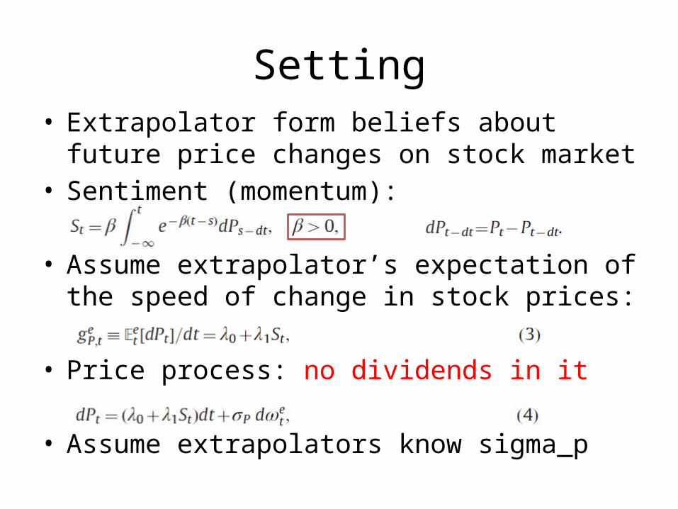
Setting• Extrapolator form beliefs about future price changes

on stock market• Sentiment (momentum):

• Assume extrapolator’s expectation of the speed of change in stock prices:

• Price process: no dividends in it

• Assume extrapolators know sigma_p

Setting

• Rational investor has correct belief about dividend process and price process.

• Know how the extrapolators form their beliefs and trade accordingly

• Both are price takers

Investors’ problem• Extrapolator:

• Same for rational trader• Clearing condition

Equilibrium

Eqm vs R – stock price• Rational:

• Equilibrium in presence of extrapolators

Eqm vs E – Stock price process• Extrapolators:

• Rational investors:

• Eqm

• Extrapolators: expected instantaneous price change depends positively on the S_t.

• Rational: depends on dividends.• In equilibrium: depends negatively on S_t.

Eqm vs E – sentiment process• Extrapolators:

• Equilibrium:

• Extrapolators: sentiment follows a random walk if lamda_1 = 1, lamda_0 = 0• In equilibrium: mean-reverting. The higher the beta, the more rapid reverts back to

mean

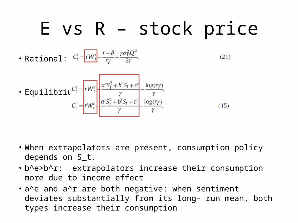
E vs R – stock price• Rational:

• Equilibrium:

• When extrapolators are present, consumption policy depends on S_t. • b^e>b^r: extrapolators increase their consumption more due to

income effect• a^e and a^r are both negative: when sentiment deviates substantially

from its long- run mean, both types increase their consumption

Empirical implication

• Predictive power of D/r –P for future price changes

• Autocorrelation of P-D/r• Volatility of price changes and of P-D/r• Autocorrelation of price changes• Correlation of consumption changes and prices

changes• Predictive power of surplus consumption• Equity premium and Sharpe ratio

Predictive power of D/r –P

• Analogous to Cochrane(2011) regressions, dividend price change can be expressed as.

• As a matter of accounting, the three regression coefficients must sum to approximately one at long horizons.– Price change on the current dividend-price change; – Dividend change on the current dividend-price change;– future dividend-price change on the current dividend-price

change

• For a fixed horizon, the predictive power of D/r - P is stronger for low μ (few rational investors)

• The predictive power of D/r - P is weaker for low β (more persistent)

Predictive power of D/r –P

• Good cash-flow news stock prices , extrapolators’ expectations , push further current stock price , D/r- P .

• But the stock market is now overvalued, subsequent price change .

• Predictability stems on extrapolators, so predictive power is stronger for low μ

• Low β implies high persistent, takes longer to correct overvaluation, lower predictive power

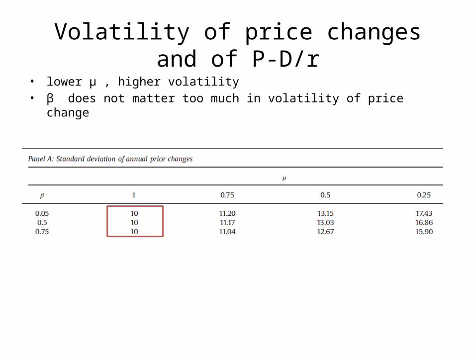
Volatility of price changes and of P-D/r• lower μ , higher volatility• β does not matter too much in volatility of price change

Volatility of price changes and of P-D/r

• A good cash-flow shock, price , extrapolators push stock prices up further. Rational investors counter act this overvaluation, but only mildly: they know that extrapolators will continue to bid.

• The larger the fraction of extrapolators (low μ) in the economy, the more excess volatility there is in price changes.

• Excess volatility is insensitive to β. Surprising?– extrapolators’ beliefs are more varying when β is high, higher β

higher volatility– However, precisely because extrapolators change their beliefs more

quickly when β is high, any mispricing will correct more quickly in this case, so rational traders trade more aggressively against the extrapolators, dampening volatility

Predictive power of surplus consumption

• Surplus consumption difference predicts subsequent price changes with negative sign

• this predictive power is strong for low μ and high β

Predictive power of surplus consumption

• Good cash-flow news -> Extrapolators' expectation -> consume more -> aggregate consumption , the surplus consumption .

• Since the stock market is overvalued at this point, the subsequent price change

• The surplus consumption difference predicts future price changes with a negative sign.

Model prediction for ratio based quantities