THE TESTABLE FLIPPED SU(5) × U(1)X

MODELS

Tianjun Li

Institute of Theoretical Physics, Chinese Academy of Sciences

I. Introduction

II. F -SU(5)

III. F -ast Proton Decay

IV. No-Scale F -SU(5) and LHC Search

V. Phenomenological Consequences

VI Conclusion

USTC, Hefei, May 20, 2011

I. INTRODUCTION

The Standard Model (SM) is a model that describes the elementary

particles in the nature and the fundamental interactions between

them.

Fundamental Interactions

Interactions Invariant Symmetry Fields Spin

Gravity Diffeomorphism Graviton 2

Strong Gauge SU(3)C Gluon 1

Weak Gauge SU(2)L W±, W 0 1

Hypercharge Gauge U(1)Y B0 1

Properties for the theories:

Gauge theory is renormalizable, and described by quantum field theory

which is consistent with both quantum mechanics and special relativity.

However, gravity theory is non-renormalizable, and we do not have a

correct quantum gravity theory.

Elementary Particles

• Three families of SM fermions:

Quarks : Q1 =

U U U

D D D

L

, (U U U )R , (D D D)R .

Leptons : L1 =

ν

E

L

, ER .

• One Higgs doublet

H =

H0

H−

.

LMSM = − 1

2g2s

TrGµνGµν − 1

2g2TrWµνW

µν

− 1

4g′2BµνB

µν + iθ

16π2TrGµνG

µν + M 2PlR

+|DµH|2 + Qii 6DQi + Uii 6DUi + Dii 6DDi

+Lii 6DLi + Eii 6DEi −λ

2

(H†H − v2

2

)2

−(hij

u QiUjH + hijd QiDjH + hij

l LiEjH + c.c.)

,

where H ≡ iσ2H∗.

The SM has 20 parameters (19 without gravity).

The Higgs potential is

VHiggs =λ

2

(H†H − v2

2

)2

,

At minimum, Higgs field has a non-zero VEV

〈H0〉 =v√2

.

All the gauge symmetries, under which H0 is charged, are broken

after Higgs mechanism.

Symmetry Breaking

• SU(2)L × U(1)Y is broken down to the U(1)em symmetry.

• W± and Z0 become massive, and γ is massless

Z0 = cos θWW 0 − sin θWB0 , γ = sin θWW 0 + cos θWB0 .

• The SM quarks and leptons obtain masses via Yukawa couplings,

except the neutrinos.

• Unknown: Higgs boson and its mass.

The SM explains existing experimental data very well, including

electroweak precision tests.

Standard Model:

• Fine-tuning problems: cosmological constant problem; gauge

hierarchy problem; strong CP problem; SM fermion masses and

mixings; ...

• Aesthetic problems: interaction and fermion unification; gauge

coupling unification; charge quantization; too many parameters; ...

Supersymmetric Standard Model:

• Solving the gauge hierarchy problem

• Gauge coupling unification

• Radiatively electroweak symmetry breaking

Large top quark mass

• Natural dark matter candidates

Neutralino, sneutrino, gravitino, ...

• Electroweak baryogenesis

• Electroweak precision: R parity

Problems in the MSSM:

• µ problem

µHuHd

• Little hierarchy problem:

Fine-tuning for the lightest CP even Higgs mass

• CP violation and EDMs

• FCNC

• Dimension-5 proton decays

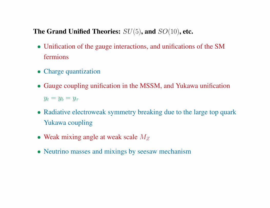
The Grand Unified Theories: SU(5), and SO(10), etc.

• Unification of the gauge interactions, and unifications of the SM

fermions

• Charge quantization

• Gauge coupling unification in the MSSM, and Yukawa unification

yt = yb = yτ

• Radiative electroweak symmetry breaking due to the large top quark

Yukawa coupling

• Weak mixing angle at weak scale MZ

• Neutrino masses and mixings by seesaw mechanism

Problems:

• Gauge symmetry breaking

• Doublet-triplet splitting problem

Higgs particles do not form complete GUT multiplet at low energy

• Proton decay problem

• Fermion mass problem

GUT relation me/mµ = md/ms

String Models:

• Calabi-Yau compactification of heterotic string theory

• Orbifold compactification of heterotic string theory

Grand Unified Theory (GUT) can be realized naturally through the

elegant E8 breaking chain: E8 ⊃ E6 ⊃ SO(10) ⊃ SU(5)

• D-brane models on Type II orientifolds

N stacks of D-branes gives us U(N) gauge symmetry: Pati-Salam

Models

• Free fermionic string model builing

Realistic models with clean particle spectra can only be constructed

at the Kac-Moody level one: the Standard-like models, Pati-Salam

models, and flipped SU(5) models.

F -Theory Model Building

• The models are constructed locally, and then the gravity should

decoupled, i.e., MGUT/MPl is a small number.

• The SU(5) and SO(10) gauge symmetries can be broken by the

U(1)Y and U(1)X /U(1)B−L fluxes.

• Gauge mediated supersymmetry breaking can be realized via

instanton effects. Gravity mediated supersymmetry breaking

predicts the gaugino mass relation.

• All the SM fermion Yuakwa couplings can be generated in the

SU(5) and SO(10) models.

• The doublet-triplet splitting problem, proton decay problem, µ

problem as well as the SM fermion masses and mixing problem can

be solved.

String Phenomenology:

• String models can solve the problems in GUTs naturally.

• Realistic string models with moduli stabilization.

• Unique predictions: testable at the LHC, ILC and other experiments.

Flipped SU(5) × U(1)X Models: a

• Doublet-triplet splitting via missing partner mechanism b.

• No dimension-five proton decay problem.

• Little hierarchy problem in string models: MString ∼ 20 × MGUT

MString = gString × 5.27 × 1017 GeV .

aS. M. Barr, Phys. Lett. B 112, 219 (1982); J. P. Derendinger, J. E. Kim and D. V. Nanopoulos, Phys. Lett. B

139, 170 (1984).bI. Antoniadis, J. R. Ellis, J. S. Hagelin and D. V. Nanopoulos, Phys. Lett. B 194, 231 (1987).

• Testable flipped SU(5) × U(1)X models: TeV-scale vector-like

particles a

• Free-fermionic string construction b

• F-theory model building c

F -SU(5) Models:

Orbifold GUTs d; Heterotic String Constructions e; ...

aJ. Jiang, T. Li and D. V. Nanopoulos, Nucl. Phys. B 772, 49 (2007).bJ. L. Lopez, D. V. Nanopoulos and K. j. Yuan, Nucl. Phys. B 399, 654 (1993).cC. Beasley, J. J. Heckman and C. Vafa, JHEP 0901, 059 (2009); J. Jiang, T. Li, D. V. Nanopoulos and D. Xie,

Phys. Lett. B 677, 322 (2009); Nucl. Phys. B 830, 195 (2010).dS. M. Barr and I. Dorsner, Phys. Rev. D 66, 065013 (2002)eA. E. Faraggi, R. S. Garavuso and J. M. Isidro, Nucl. Phys. B 641, 111 (2002).

II. F -SU(5) MODELS

• The gauge group SU(5) × U(1)X can be embedded into SO(10)

model.

• Generator U(1)Y ′ in SU(5)

TU(1)Y′ = diag

(−1

3,−1

3,−1

3,1

2,1

2

).

• Hypercharge

QY =1

5(QX − QY ′) .

• SM fermions

Fi = (10, 1), fi = (5,−3), li = (1, 5) ,

Fi = (Qi, Dci , N

ci ), f i = (U c

i , Li), li = Eci .

• Higgs particles:

H = (10, 1), H = (10,−1), h = (5,−2), h = (5, 2) ,

H = (QH, DcH, N c

H) , H = (QH , DcH, N

cH) ,

h = (Dh, Dh, Dh, Hd) , h = (Dh, Dh, Dh, Hu) .

Symmetry Breaking:

• Superpotential

W GUT = λ1HHh + λ2HHh + Φ(HH − M 2H) .

• There is only one F-flat and D-flat direction along the N cH and N

cH

directions: < N cH >=< N

cH >= MH.

• The doublet-triplet splitting due to the missing partner mechanism

The superfields H and H are eaten and acquire large masses via the

supersymmetric Higgs mechanism, except for DcH and D

cH . And the

superpotential λ1HHh and λ2HHh couple the DcH and D

cH with the

Dh and Dh, respectively, to form the massive eigenstates with

masses 2λ1 < N cH > and 2λ2 < N

cH >.

• No dimension-5 proton decay problem.

Because the triplets in h and h only have small mixing through the µ

term, the Higgsino-exchange mediated proton decay are negligible.

F -SU(5) Models:

• To achieve the string scale gauge coupling unification, we introduce

sets of vector-like particles in complete SU(5) × U(1)X multiplets,

whose contributions to the one-loop beta functions of the U(1)Y ,

SU(2)L and SU(3)C gauge symmetries, ∆b1, ∆b2 and ∆b3

respectively, satisfy ∆b1 < ∆b2 = ∆b3.

• To avoid the Landau pole problem for the gauge couplings, we can

only introduce the following two sets of vector-like particles around

the TeV scale, which could be observed at the LHC

Z1 : XF = (10, 1) , XF = (10,−1) ;

Z2 : XF , XF , Xl = (1,−5) , Xl = (1, 5) .

• We define the flipped SU(5) × U(1)X models with Z1 and Z2 sets

of vector-like particles as Type I and Type II models, respectively.

Models MV MS M23 gU MU

Type II 200 360 1.21 × 1016 1.289 6.79 × 1017

Type II 200 1000 1.25 × 1016 1.194 6.29 × 1017

Type II 1000 360 1.13 × 1016 1.207 1.20 × 1018

Type II 1000 1000 1.18 × 1016 1.143 9.33 × 1017

Type II 2.0 × 104 800 1.15 × 1016 1.051 5.54 × 1017

Table 1: Mass scales in GeV unit and gauge couplings in the F-SU(5) models for

gauge coupling unification.

0

20

40

60

103

107

1011

1015

Model IA

MV

= 1000 GeV

MS = 800 GeV

α-1

3

α-1

2

α-1

1

α′-1

1

α-1

5

µ (GeV)

α-1

Figure 1: Gauge coupling unification in the Type II model.

III. F -AST PROTON DECAY

Proton decay experiments:

• Super-Kamiokande, a 50-kiloton (kt) water Cherenkov detector, has

set the current lower bounds of 8.2 × 1033 and 6.6 × 1033 years at the

90% confidence level for the partial lifetimes in the p → e+π0 and

p → µ+π0 modes.

• Hyper-Kamiokande is a proposed 1-Megaton detector, about 20

times larger volumetrically than Super-Kamiokande, which we can

expect to explore partial lifetimes up to a level near 2 × 1035 years

for p → e+π0 across a decade long run.

• The proposal for the DUSEL experiment features both 500 kt water

Cherenkov and 100 kt liquid Argon detectors, with the stated goal of

probing partial lifetimes into the order of 1035 years for both the

p → e+π0 and p → K+νµ channels.

• LAGUNA is a European collaboration which is considering three

possible technologies; water Cherenkov, liquid argon or liquid

scintillators. These detectors, if built, have similar goals to any

DUSEL detector, i.e., to reach a lifetime sensitivity of 1035 years.

Proton decay in flipped SU(5) × U(1):

• After integrating out the heavy gauge boson fields, we obtain the

effective dimension-six operator for proton decay

L =g2

23ǫijk

2M 232

[((dc

k cos θc + sck sin θc)γ

µPLuj) × (uiγµPLeL) + h.c.]

.

• The decay amplitude is proportional to the overall normalization of

the proton wave function at the origin. Relevant matrix elements

have been calculated in a lattice approach with quoted errors below

10%, corresponding to an uncertainty of less than 20% in the proton

partial lifetime. Thus, this uncertainty is negligible.

• Proton lifetime is sensitive to M23 and g23

τ (p → e+π0) ∼(

M23

g23

)4

.

Proton decay: a

• We consider two-loop RGE running for gauge couplings and

one-loop RGE running for top and bottom Yukawa couplings.

• For the light MZ-scale threshold corrections from the

supersymmetric particles, we consider the CMSSM benchmark

scenarios, which respect all the available experimental constraints.

• For the M23 scale threshold corrections from the triplet Higgs fields

and heavy gauge fields of SU(5), from naturalness we assume

√λ1λ2

3≤ g23 ≤ 3

√λ1λ2 .

• Because XF and XF form complete SU(5)×U(1)X multiplets and

Xl and Xl are SU(5) singlets, we can assume degeneracy of these

vector-like particles’ masses at a central value of 1 TeV.

aT. Li, D. V. Nanopoulos and J. W. Walker, arXiv:0910.0860 [hep-ph]; arXiv:1003.2570 [hep-ph].

105 1010 1015

0.00

0.02

0.04

0.06

0.08

0.10

0.12

@GeVD

Αi

Figure 2: Gauge coupling unification in the minimal (red dashed lines) and Type II

(green dashed lines) flipped SU(5) × U(1)X models for benchmark scenario B′.

Model g1 g23 M23 (GeV) τp (Years)

Minimal 0.70 0.72 5.8 × 1015 4.3 × 1034

Type I 0.75 1.21 6.8 × 1015 1.0 × 1034

Type II 0.87 1.20 6.8 × 1015 1.0 × 1034

Table 2: Proton decay for benchmark scenario B′.

The central prediction of the proton partial lifetime for the minimal,

Type I and Type II models is well below 1035 years, within the reach of

the future Hyper-Kamiokande and DUSEL experiments. However, the

uncertainty from heavy threshold corrections ever threatens to undo this

promising result.

Uncertainty at M Z Uncertainty at M Z Heavy Thresholds

K'

J'

I'

H'

G'

F'

E'

D'

C'

B'

A'

0.2 0.5 1.0 2.0 5.0

1035 @YD

Figure 3: Including uncertainties from threshold corrections at the MZ and M23 scales,

the proton partial lifetime in the minimal flipped SU(5) × U(1)X model.

Uncertainty at M Z Uncertainty at M Z Heavy Thresholds

K'

J'

I'

H'

G'

F'

E'

D'

C'

B'

A'

0.05 0.1 0.2 0.5 1.0 2.0

1035 @YD

Figure 4: Including uncertainties from threshold corrections at the MZ and M23 scales,

the proton partial lifetime in the Type II flipped SU(5) × U(1)X model.

Summary on Proton Decay:

• In the minimal model, the central partial lifetime is in the range of

4 − 7 × 1034 years for benchmark scenarios from A′ to I ′, and about

1 − 2 × 1035 years for benchmark scenarios J ′ and K ′. However, the

uncertainties from the heavy threshold corrections at M23 are indeed

quite large. Proton decay appears to be within the reach of the future

Hyper-Kamiokande, DUSEL, and LAGUNA experiments if the

heavy threshold corrections are more modest.

• For Type II flipped SU(5) × U(1)X model, the central values for the

partial lifetime are about 1 − 2 × 1034 years for benchmark scenarios

from A′ to I ′, and about 2 − 3 × 1034 years for benchmark scenarios

J ′ and K ′. Even including uncertainties from the light and heavy

threshold corrections, the lifetime is still less than 2 − 3 × 1035 years

for all scenarios considered. A strong majority of the parameter

space for proton decay does indeed appear to be within the reach of

the future Hyper-Kamiokande and DUSEL experiments for the Type

II flipped SU(5) × U(1)X model. This basic conclusion holds also

for the Type I flipped SU(5) × U(1)X model.

IV. NO-SCALE F -SU(5)

No-Scale Supergravity: a

• The vacuum energy vanishes automatically due to the suitable

Kahler potential;

• At the minimum of the scalar potential, there are flat directions

which leave the gravitino mass M3/2 undertermined;

• The super-trace quantity StrM2 is zero at the minimum.

K = −3ln(T + T −∑

i

ΦiΦi) .

aE. Cremmer, S. Ferrara, C. Kounnas and D. V. Nanopoulos, Phys. Lett. B 133, 61 (1983); A. B. Lahanas and

D. V. Nanopoulos, Phys. Rept. 145, 1 (1987).

No-Scale Supergravity:

• mSUGRA: M1/2, M0, A, tan β

• No-Scale boundary condition: M1/2 6= 0, M0 = A = Bµ = 0

• Natural solution to CP violation and FCNC problem.

• Disfavored by phenomenology: M0 = 0 at traditional GUT scale

• No-scale F -SU(5)

No-scale supergravity can be realized in the compactification of the

weakly coupled heterotic string theory a and the compactification of

M-theory on S1/Z2 at the leading order b.

aE. Witten, Phys. Lett. B 155, 151 (1985).bT. Li, J. L. Lopez and D. V. Nanopoulos, Phys. Rev. D 56, 2602 (1997).

Constraints:

• The WMAP 2σ measurements of the cold dark matter density:

0.1088 ≤ Ωχ ≤ 0.1158.

• The experimental limits on the Flavor Changing Neutral Current

(FCNC) process for b → sγ:

2.86 × 10−4 ≤ Br(b → sγ) ≤ 4.18 × 10−4.

• The anomalous magnetic moment of the muon, gµ − 2:

11 × 10−10 < aµ < 44 × 10−10.

• The process B0s → µ+µ−: Br(B0

s → µ+µ−) < 5.8 × 10−8.

• The LEP limit on the lightest CP-even Higgs boson mass mh ≥ 114

GeV.

No-Scale F -SU(5): a

• M0 = A = Bµ = 0, tan β is a function of M1/2 and µ.

• Choosing tan β (equivalent to µ) and M1/2 as free parameters, we

determine the no-scale parameter space by requiring that Bµ = 0.

• Taking MV = 1 TeV, the Bµ(MF) = 0 contour runs sufficiently

perpendicular to the WMAP strip, which gives the observed dark

matter density.

aT. Li, J. A. Maxin, D. V. Nanopoulos and J. W. Walker, arXiv:1007.5100 [hep-ph].

Figure 5: Viable parameter space in the tan β − M1/2 plane.

No-Scale F -SU(5): a

• To realize radiative EWSB and match the observed CDM density,

tan β ≃ 15 (equivalent to fix µ).

• Bµ at MZ is very sensitive to mt, but not sensitive to α3 and MZ .

• We choose M1/2, MV , mt as free parameters and require that Bµ = 0

at the GUT scale.

aT. Li, J. A. Maxin, D. V. Nanopoulos and J. W. Walker, arXiv:1009.2981 [hep-ph].

455460465470475480

700

800

900

1000

173.0

173.5

174.0

174.5

481

> WMAP 7-yr Br(b s )

mt

M1/2

MV

|B (MF )|<1 Hyper-surface (thickness 0.3 GeV & inclined 0.2 above M

1/2-M

V plane)

Golden Strip WMAP 7-yr a Br(b s ) |B (MF )|<1 Hyper-surface

a1020

691

455

173.0

174.4

Figure 6: With tanβ ≃ 15 fixed by WMAP-7, the residual parameter volume is three

dimensional in (M12, MV, mt), with the |Bµ(MF)| ≤ 1 (slightly thickened) surface

forming a shallow (0.2) incline above the (M12, MV) plane.

450455

460465

470475

4804850

10002000

30004000

0

10

20

30

40

50

M1/2M

V

|B ( MF )|

173.0

173.3

173.6

173.8

174.1

174.4

Figure 7: The Bµ = 0 target for variations in (M1/2, MV), with tan β = 15. The

specific mt which is required to minimize |Bµ(MF)| is annotated along the solution

string.

Figure 8: With tanβ ≃ 15 fixed by WMAP-7, the residual parameter volume is three

dimensional in (M12, MV, mt), with the |Bµ(MF)| ≤ 1 (slightly thickened).

Results:

• A highly non-trivial “golden strip” with tan β ≃ 15,

mt = 173.0-174.4 GeV, M1/2 = 455-481 GeV, and

MV = 691-1020 GeV.

• Postdicting the correct top quark mass.

• The predicted range of MV is testable at the LHC.

• The partial lifetime for proton decay in the leading (e|µ)+π0

channels falls around 4.6 × 1034 Y.

• Bµ = 0 constraint is highly non-trivial.

• The golden strip is further consistent with the CDMSII and

Xenon100 upper limits, with the spin-independent cross section

extending from σSI = 1.3-1.9 × 10−10 pb. Likewise, the allowed

region satisfies the Fermi-LAT space telescope constraints with the

photon-photon annihilation cross section 〈σv〉γγ ranging from

〈σv〉γγ = 1.5-1.7 × 10−28 cm3/s.

Benchmark Point:

Table 3: Spectrum (in GeV) for the benchmark point. Here, M1/2 = 464 GeV, MV =

850 GeV, mt = 173.6 GeV, Ωχ = 0.112, σSI = 1.7 × 10−10 pb, and 〈σv〉γγ = 1.7 ×10−28 cm3/s. The central prediction for the p→ (e|µ)+π0 proton lifetime is 4.6 × 1034

years. The lightest neutralino is 99.8% Bino.

χ01 96 χ±

1 187 eR 153 t1 499 uR 975 mh 120.6

χ02 187 χ±

2 849 eL 519 t2 929 uL 1062 mA,H 946

χ03 845 νe/µ 513 τ1 105 b1 880 dR 1018 mH± 948

χ04 848 ντ 506 τ2 514 b2 992 dL 1065 g 629

Super-No-Scale F -SU(5):

• M1/2 as a modulus parameter.

• Fixing MV , mt, and µ at MF , for a particular M1/2, we can

determine an EWSB vacuum with potential Vmin.

• Super-No-Scale Condition: minimum minimorum, dVmin/dM1/2 = 0

• Moduli Stabilization and Complete Solution to the Gauge Hiearchy

Problem

Super-No-Scale F -SU(5):

• Fixing MZ: a

• Fixing MV , mt, and µ at MU : M32b

Dynamically Determination of M1/2 and the electroweak scale in the

Golden Strip.

aT. Li, J. A. Maxin, D. V. Nanopoulos and J. W. Walker, arXiv:1010.4550 [hep-ph].bT. Li, J. A. Maxin, D. V. Nanopoulos and J. W. Walker, arXiv:1101.2197 [hep-ph].

0

200

400

600800

1000

5

10

1520

2530

800

1000

1200

1400

1600

Electroweak Vacua (B (MF)=0)

Gold Point

Minimum Minimorum

tan

Vmin(h)

M1/2

Figure 9: Dynamical determination of M1/2: fixing MZ .

91.00

91.25

91.5091.75

92.0092.25

92.5092.75

93.00

450

452

454

456

458

460

750

760

770

780

790

M1/2

Vmin

(h)

MZ

Minimum Minimorum

Figure 10: Dynamical determination of M1/2: fixing MV , mt, and µ at MU .

LHC Search at the Early Run: a

• Vector-like particles are difficult.

• Specific feature: Lighter stop and gluino.

• Looking for the multiple jets: four tops, > 8 jets.

• LHC: 7 TeV and 1-3 fb−1.

aT. Li, J. A. Maxin, D. V. Nanopoulos and J. W. Walker, arXiv:1103.2362 [hep-ph], and arXiv:1103.4160

[hep-ph].

LHC Search: Benchmark Point

Table 4: Spectrum (in GeV) for M1/2 = 410 GeV, MV = 1 TeV, mt = 174.2 GeV, tanβ

= 19.5. Here, Ωχ = 0.11 and the lightest neutralino is 99.8% bino.

χ0

176 χ±

1165 eR 157 t1 423 uR 865 mh 120.4

χ0

2165 χ±

2756 eL 469 t2 821 uL 939 mA,H 814

χ0

3752 νe/µ 462 τ1 85 b1 761 dR 900 mH± 820

χ0

4755 ντ 452 τ2 462 b2 864 dL 942 g 561

Property of Particle Spectra:

• Both the particle spectra and the sparticle branch ratio are similar in

the (updated) “Golden Strip” up to a small rescale since M1/2 is the

only supersymmetry breaking parameter.

• Light gluino due to b3 = 0.

• The distinctive mass pattern: mt1< mg < mq.

• Different from the ten “Snowmass Points and Slopes” (SPS)

benchmark points.

Collider Physics:

• MadGraph and MadEvent: Low order Feymann Diagram and Monte

Carlo simulated parton level scattering events.

• PYTHIA: the cascaded fragmentation and hadronization of these

events into final state showers of photons, leptons, and mixed jets.

• PGS4: simulating the physical detector environment.

• MLM matching: avoid double counting.

• CTEQ6L1: parton distribution functions .

• The updated b-tag efficiency ∼60%.

Event Veto Conditions:

• pT < 100 GeV for the two leading jets.

• pT < 350 GeV for all jets.

• Pseudorapidity |η| > 2 for the leading jet.

• Missing energy /ET < 150 GeV.

• Isolated photon with pT > 25 GeV.

• Isolated electron or muon with pT > 10 GeV.

• Any single jet with |η| > 3

Decaying Chains:

• g → t1t → ttχ01 → W+W−bbχ0

1.

• g → t1t → btχ+1 → W−bbτ+

1 ντ → W−bbτ+ντ χ01.

• g → t1t → ttχ01.

• g → t1t → btχ−1 .

2 3 4 5 6 7 8 9 10 11 12 13 14 15 16

0

20

40

60

80

2 3 4 5 6 7 8 9 10 11 12 13 14 15 16

0

4

8

12

16

20

2 3 4 5 6 7 8 9 10 11 12 13 14 15 16

0

10

20

30

40

50

601fb-1@7TeV

Number of Jets / Event

Single Jet pT > 20 GeV

F-SU(5) with vector-like particles mSUGRA Snowmass Benchmark SP3 Standard Model tt + jets

Install cut @ 9 jets

Num

ber o

f Eve

nts

CMS Cuts (arXiv:1101.1628 [hep-ex])

1fb-1@7TeV

1fb-1@7TeV

Single Jet pT > 10 GeV

Install cut @ 11 or 12 jets

Figure 11: Distribution of events per number of jets. For clarity of the peaks, polyno-

mials have been fitted over the histograms. PT > 20 GeV.

500 1000 1500 2000 2500 3000 35000

5

10

15

20

25

30 9 jets

Eve

nts

/ 200

GeV

HT (GeV)

F-SU(5) with vector-like particles mSUGRA Snowmass Benchmark SP3 Standard Model tt + jets

1 fb-1 @ 7 TeVpjT > 20 GeV

Figure 12: Counts for events with ≥ 9 jets. HT =∑Njet

i=1Eji

T .

Table 5: Total number of events for 1 fb−1 and√

s = 7 TeV. Minimum pT for a single

jet is pT > 20 GeV.

F -SU(5) SP3 tt + jets

Events 93.2 2.4 10

S√B

29.5 0.76

The benchmark point can be tested at the early LHC run.

PHENOMENOLOGICAL CONSEQUENCES

• The lightest CP-even Higgs boson mass is larger than the MSSM

due to the additional Yukawa interactions between the MSSM Higgs

fields and these vector-like particles a

−L = ydXFXFXFh + yu

XFXFXFh .

• The neutrino masses and mixings can be generated via seesaw

mechanism. And the observed baryon asymmetry can be explained

via leptogenesis.

aY. J. Huo, T. Li, D. V. Nanopoulos and C. L. Tong, in preparation.

• We can naturally have the hybrid inflation where Φ is the inflaton

field. The inflation scale is related to the scale M23. Because M23 is

at least one order smaller than MU , we solve the monopole problem.

Interestingly, we can generate the correct cosmic primordial density

fluctuations a

δρ

ρ∼

(M23

g23MPl

)2

∼ 1.7 × 10−5 .

aB. Kyae and Q. Shafi, Phys. Lett. B 635, 247 (2006).

115

120

125

130

135

140

145

150

155

0 5 10 15 20 25 30 35 40

Mh/G

eV

tan β

MS = 800GeV, MV = 400GeV, Yxd = Yxu

Model IModel IIModel IIIModel IVModel V

For MS = 800 GeV and MV = 800 GeV, the lightest CP-even Higgs

boson mass versus tan β.

CONCLUSION

F -SU(5)

• These models can be realized in free fermionic string constructions

and F-theory model building.

• Lighter stop and gluino can be observed at the LHC early run.

• The models may be tested in the early LHC run. And the TeV-scale

vector-like particles can be produced and observed at the next LHC

run.

• The proton decay p → e+π0 from the heavy gauge boson exchange

is within the reach of the future DUSEL and Hyper-Kamiokande

experiments for a majority of the most plausible parameter space.

• A strong correlation between the most exciting particle physics

experiments of the coming decade.

• The phenomenological consequences are pretty interesting.