Www.themegallery.com Chapter 4 The Monetary and Portfolio Balance Approaches to External Balance.
40
www.themegallery.com Chapter 4 The Monetary and Portfolio Balance Approaches to External Balance
-
Upload
wendy-cobb -
Category
Documents
-
view
218 -
download
2
Transcript of Www.themegallery.com Chapter 4 The Monetary and Portfolio Balance Approaches to External Balance.

www.themegallery.com
Chapter 4
The Monetary and Portfolio Balance Approaches to External Balance

Learning Objectives
Show how the supply and demand for money can affect a country’s balance of payments and exchange rate.
Describe how other financial assets besides money can influence exchange rates and international payments positions.
Explain how a changing exchange rate can overshoot its new equilibrium value.
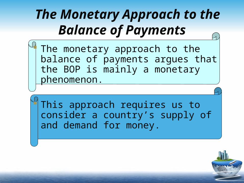
The Monetary Approach to the Balance of Payments The monetary approach to the
balance of payments argues that the BOP is mainly a monetary phenomenon.
This approach requires us to consider a country’s supply of and demand for money.
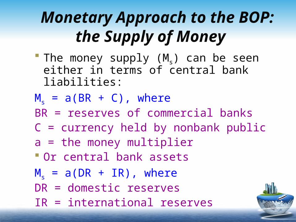
Monetary Approach to the BOP: the Supply of Money The money supply (Ms) can be seen
either in terms of central bank liabilities:
Ms = a(BR + C), where BR = reserves of commercial banksC = currency held by nonbank publica = the money multiplier Or central bank assetsMs = a(DR + IR), whereDR = domestic reservesIR = international reserves
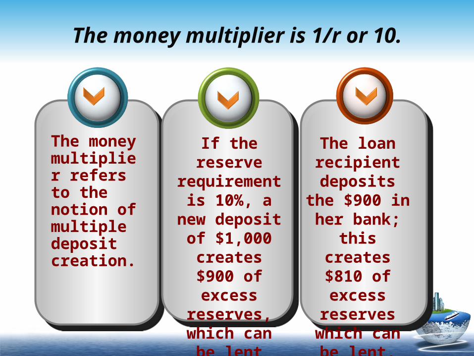
The money multiplier refers to the notion of multiple deposit creation.
If the reserve requirement is
10%, a new deposit of
$1,000 creates $900 of excess
reserves, which can be
lent out.
The loan recipient
deposits the $900 in her bank; this
creates $810 of excess reserves
which can be lent, etc.
The money multiplier is 1/r or 10.

Anything that increases the assets of the central bank (or equivalently, its liabilities) allows the money supply to expand via the multiplier process.
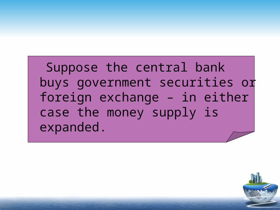
Suppose the central bank buys
government securities or foreign exchange – in either case the money supply is expanded.
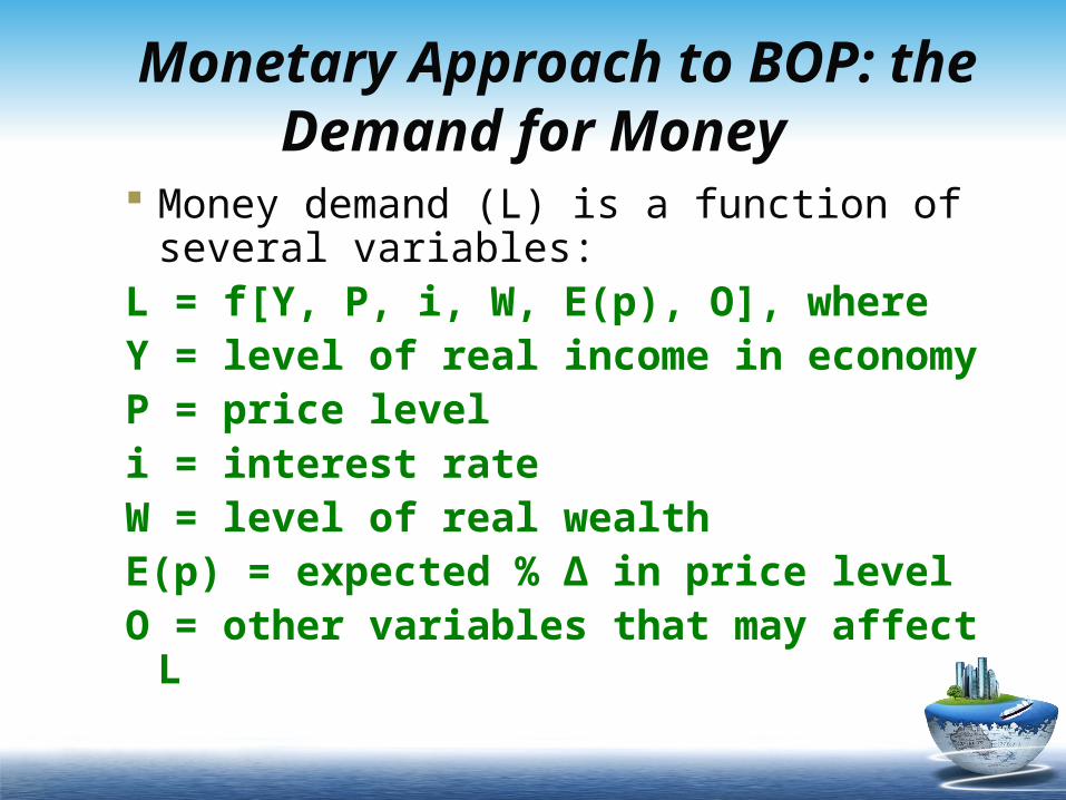
Monetary Approach to BOP: the Demand for Money
Money demand (L) is a function of several variables:
L = f[Y, P, i, W, E(p), O], where Y = level of real income in economyP = price leveli = interest rateW = level of real wealthE(p) = expected % Δ in price levelO = other variables that may affect L
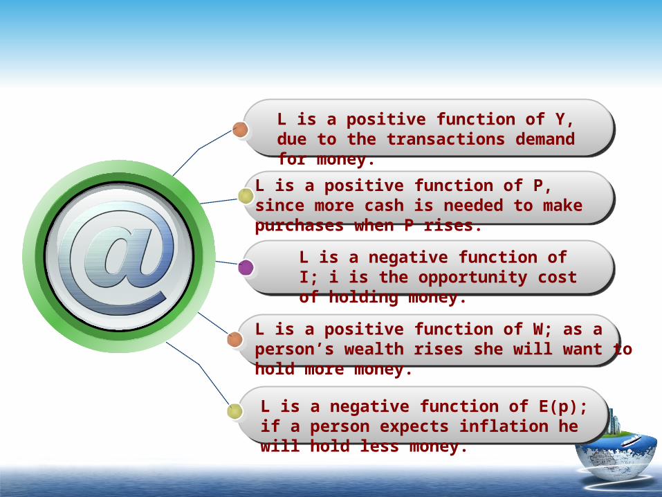
L is a positive function of Y, due to the transactions demand for money.
L is a positive function of P, since more cash is needed to make purchases when P rises.
L is a negative function of I; i is the opportunity cost of holding money.
L is a positive function of W; as a person’s wealth rises she will want to hold more money.
L is a negative function of E(p); if a person expects inflation he will hold less money.
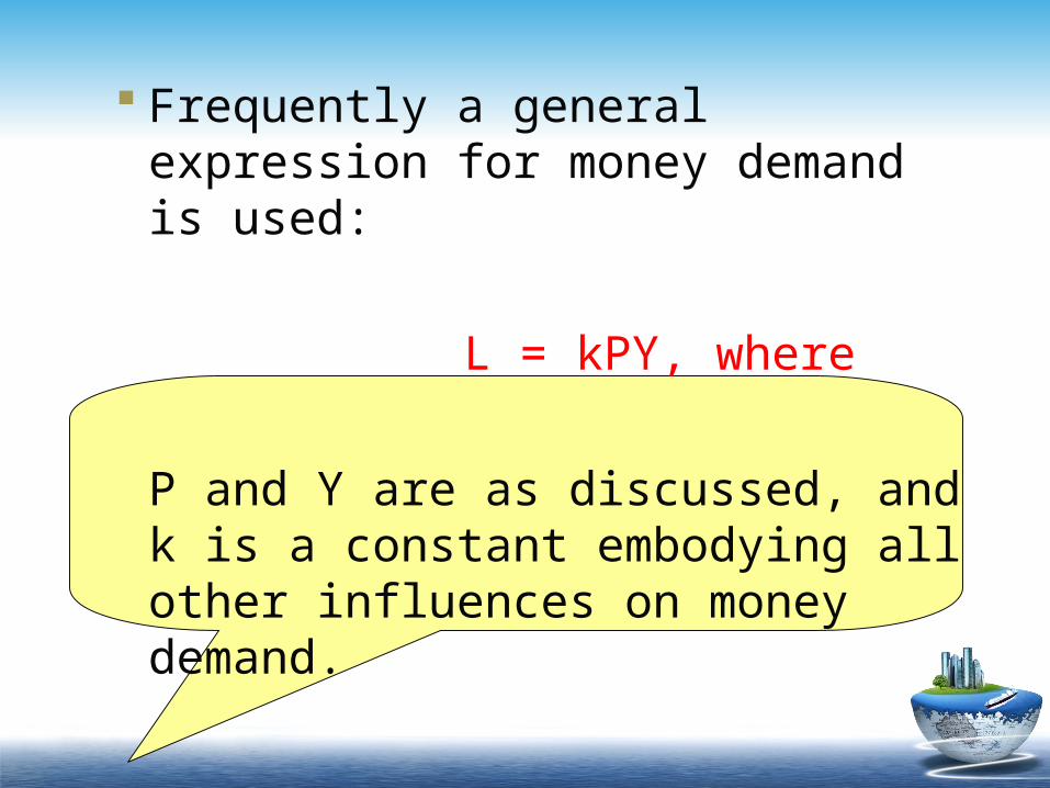
Frequently a general expression for money demand is used:
L = kPY, where
P and Y are as discussed, and k is a constant embodying all other influences on money demand.
Monetary Approach to BOP: Monetary Equilibrium
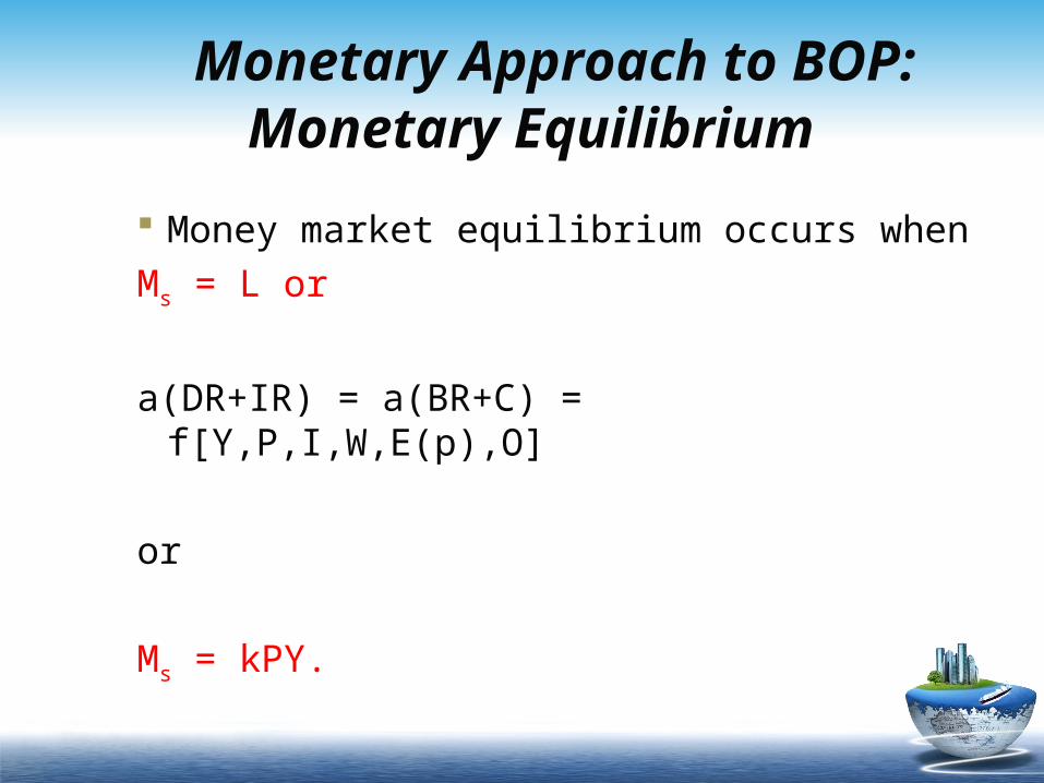
Money market equilibrium occurs when Ms = L or
a(DR+IR) = a(BR+C) = f[Y,P,I,W,E(p),O]
or
Ms = kPY.
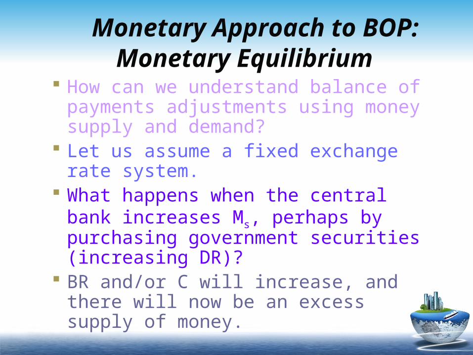
Monetary Approach to BOP: Monetary Equilibrium How can we understand balance of
payments adjustments using money supply and demand?
Let us assume a fixed exchange rate system.
What happens when the central bank increases Ms, perhaps by purchasing government securities (increasing DR)?
BR and/or C will increase, and there will now be an excess supply of money.
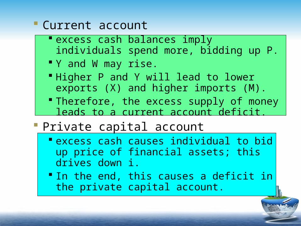
Current account excess cash balances imply individuals
spend more, bidding up P. Y and W may rise. Higher P and Y will lead to lower exports (X)
and higher imports (M). Therefore, the excess supply of money leads
to a current account deficit. Private capital account
excess cash causes individual to bid up price of financial assets; this drives down i.
In the end, this causes a deficit in the private capital account.
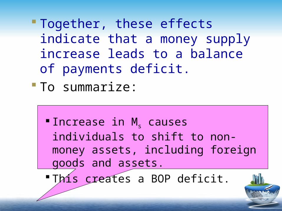
Together, these effects indicate that a money supply increase leads to a balance of payments deficit.
To summarize:
Increase in Ms causes individuals to shift to non-money assets, including foreign goods and assets.
This creates a BOP deficit.
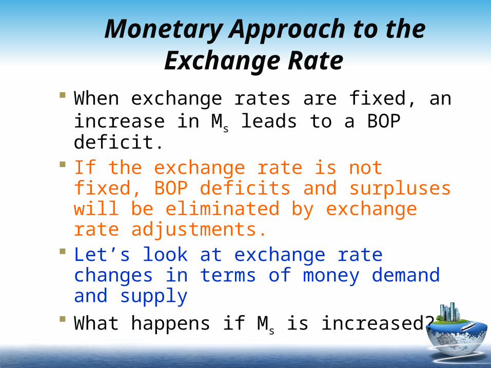
Monetary Approach to the Exchange Rate
When exchange rates are fixed, an increase in Ms leads to a BOP deficit.
If the exchange rate is not fixed, BOP deficits and surpluses will be eliminated by exchange rate adjustments.
Let’s look at exchange rate changes in terms of money demand and supply
What happens if Ms is increased?
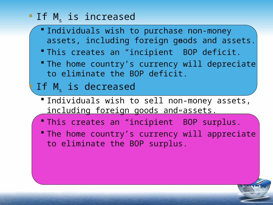
If Ms is increased Individuals wish to purchase non-money
assets, including foreign goods and assets. This creates an “incipient” BOP deficit. The home country’s currency will depreciate
to eliminate the BOP deficit.
If Ms is decreased Individuals wish to sell non-money assets,
including foreign goods and assets. This creates an “incipient” BOP surplus. The home country’s currency will appreciate
to eliminate the BOP surplus.
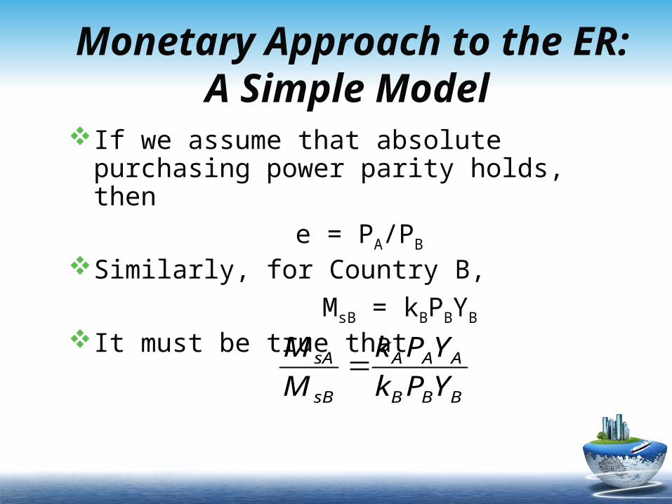
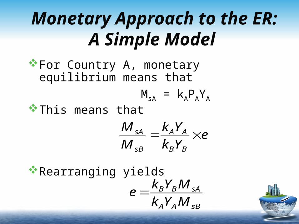
Monetary Approach to the ER: A Simple Model
If we assume that absolute purchasing power parity holds, then
e = PA/PB
Similarly, for Country B, MsB = kBPBYB
It must be true that
BBB
AAA
sB
sA
YPk
YPk
M
M
Monetary Approach to the ER: A Simple Model
For Country A, monetary equilibrium means that
MsA = kAPAYA
This means that
Rearranging yields
eYk
Yk
M
M
BB
AA
sB
sA
sBAA
sABB
MYk
MYke
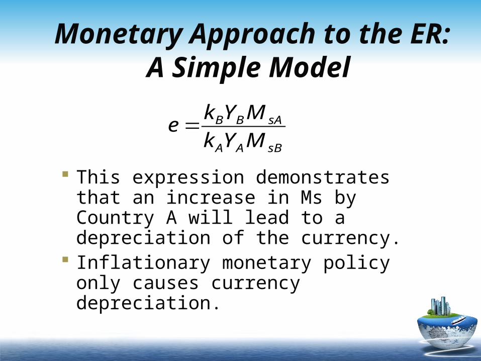
Monetary Approach to the ER: A Simple Model
This expression demonstrates that an increase in Ms by Country A will lead to a depreciation of the currency.
Inflationary monetary policy only causes currency depreciation.
sBAA
sABB
MYk
MYke
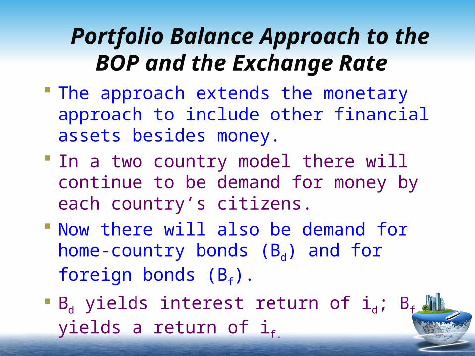
Portfolio Balance Approach to the BOP and the Exchange Rate The approach extends the monetary
approach to include other financial assets besides money.
In a two country model there will continue to be demand for money by each country’s citizens.
Now there will also be demand for home-country bonds (Bd) and for foreign bonds (Bf).
Bd yields interest return of id; Bf yields a return of if.
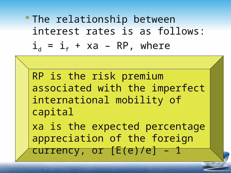
The relationship between interest rates is as follows:
id = if + xa – RP, where
RP is the risk premium associated with the imperfect international mobility of capitalxa is the expected percentage appreciation of the foreign currency, or [E(e)/e] – 1
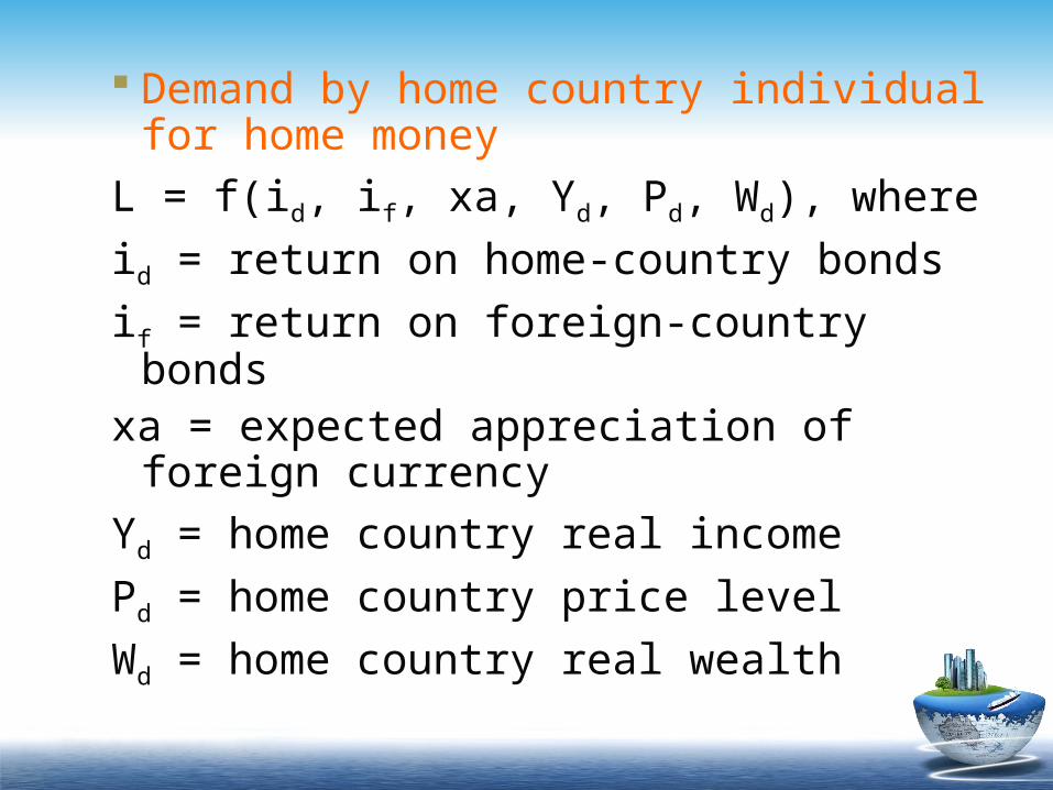
Demand by home country individual for home money
L = f(id, if, xa, Yd, Pd, Wd), where
id = return on home-country bonds
if = return on foreign-country bondsxa = expected appreciation of
foreign currencyYd = home country real income
Pd = home country price level
Wd = home country real wealth
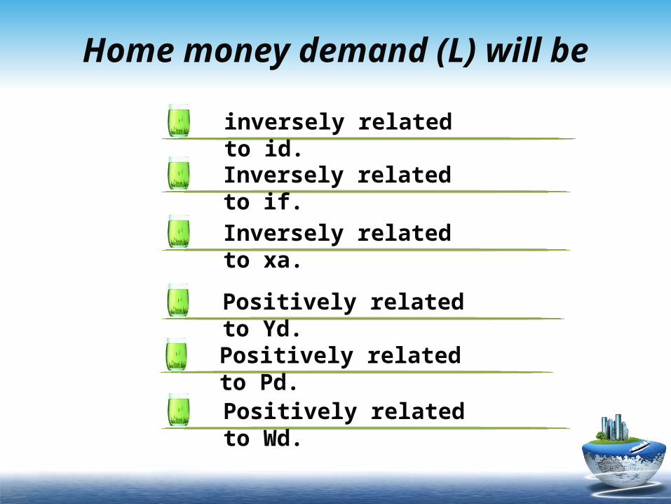
inversely related to id.
Inversely related to if.
Inversely related to xa.
Positively related to Yd.
Home money demand (L) will be
Positively related to Pd.Positively related to Wd.
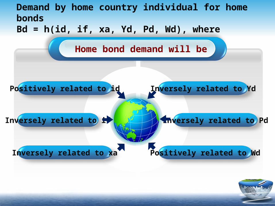
Inversely related to YdPositively related to id
Inversely related to PdInversely related to if
Positively related to WdInversely related to xa
Home bond demand will be
Demand by home country individual for home bondsBd = h(id, if, xa, Yd, Pd, Wd), where
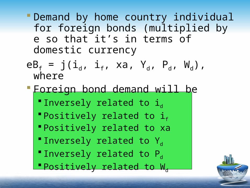
Demand by home country individual for foreign bonds (multiplied by e so that it’s in terms of domestic currency
eBf = j(id, if, xa, Yd, Pd, Wd), where Foreign bond demand will be
Inversely related to id Positively related to if Positively related to xa Inversely related to Yd
Inversely related to Pd Positively related to Wd
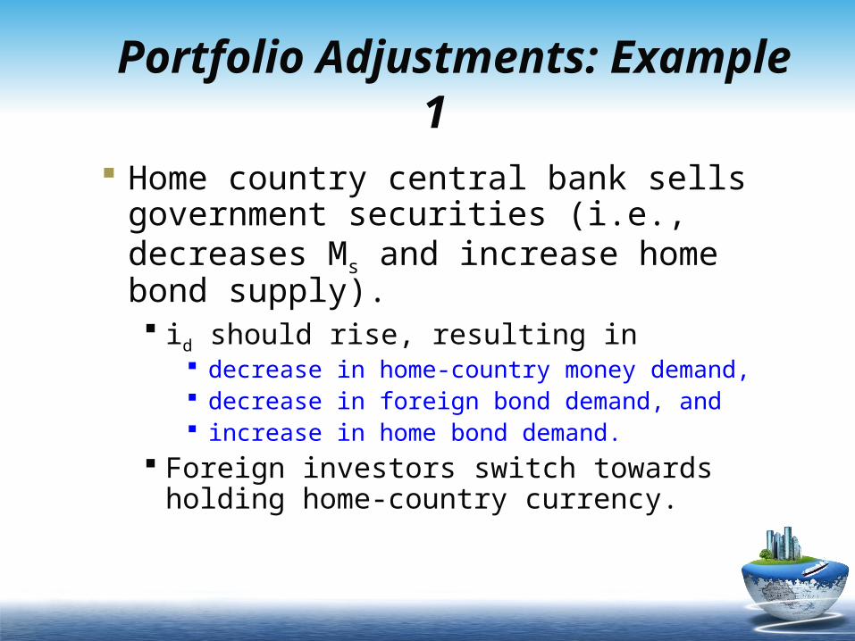
Portfolio Adjustments: Example 1
Home country central bank sells government securities (i.e., decreases Ms and increase home bond supply). id should rise, resulting in
decrease in home-country money demand, decrease in foreign bond demand, and increase in home bond demand.
Foreign investors switch towards holding home-country currency.
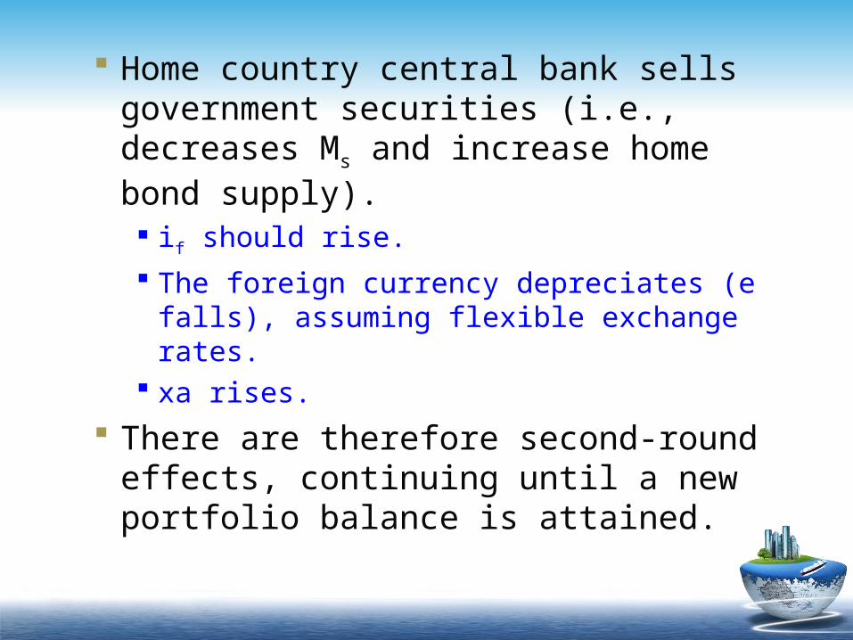
Home country central bank sells government securities (i.e., decreases Ms and increase home bond supply). if should rise. The foreign currency depreciates (e falls),
assuming flexible exchange rates. xa rises.
There are therefore second-round effects, continuing until a new portfolio balance is attained.
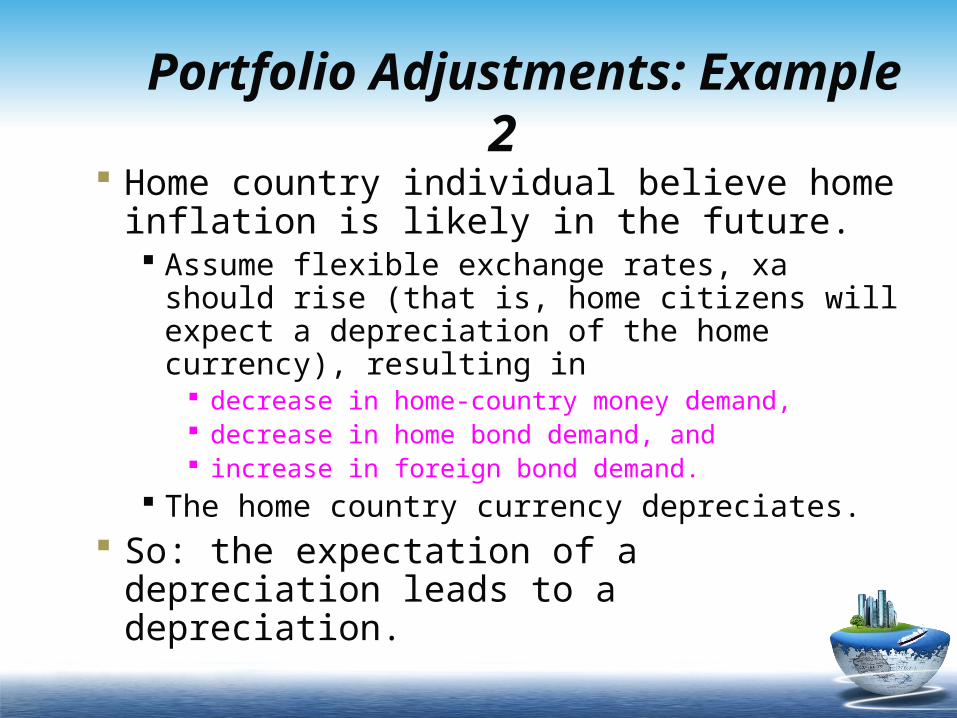
Portfolio Adjustments: Example 2
Home country individual believe home inflation is likely in the future. Assume flexible exchange rates, xa should
rise (that is, home citizens will expect a depreciation of the home currency), resulting in
decrease in home-country money demand, decrease in home bond demand, and increase in foreign bond demand.
The home country currency depreciates. So: the expectation of a depreciation
leads to a depreciation.
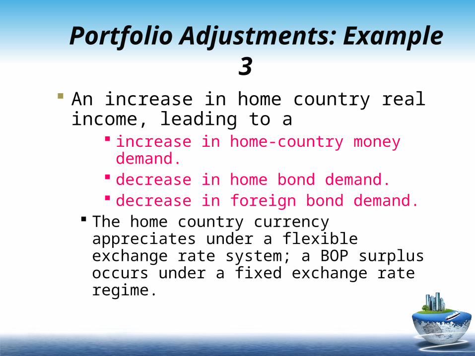
Portfolio Adjustments: Example 3
An increase in home country real income, leading to a
increase in home-country money demand.
decrease in home bond demand. decrease in foreign bond demand.
The home country currency appreciates under a flexible exchange rate system; a BOP surplus occurs under a fixed exchange rate regime.
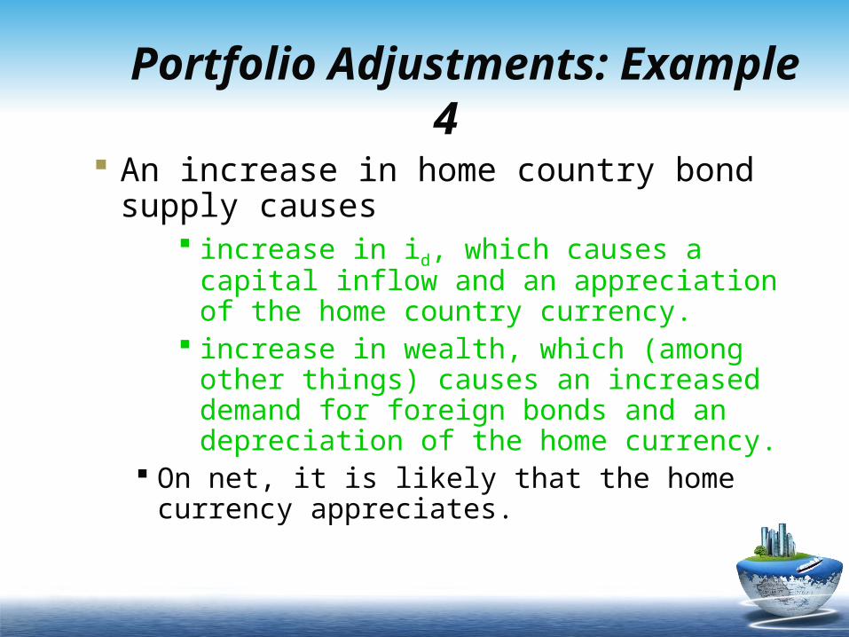
Portfolio Adjustments: Example 4
An increase in home country bond supply causes
increase in id, which causes a capital inflow and an appreciation of the home country currency.
increase in wealth, which (among other things) causes an increased demand for foreign bonds and an depreciation of the home currency.
On net, it is likely that the home currency appreciates.
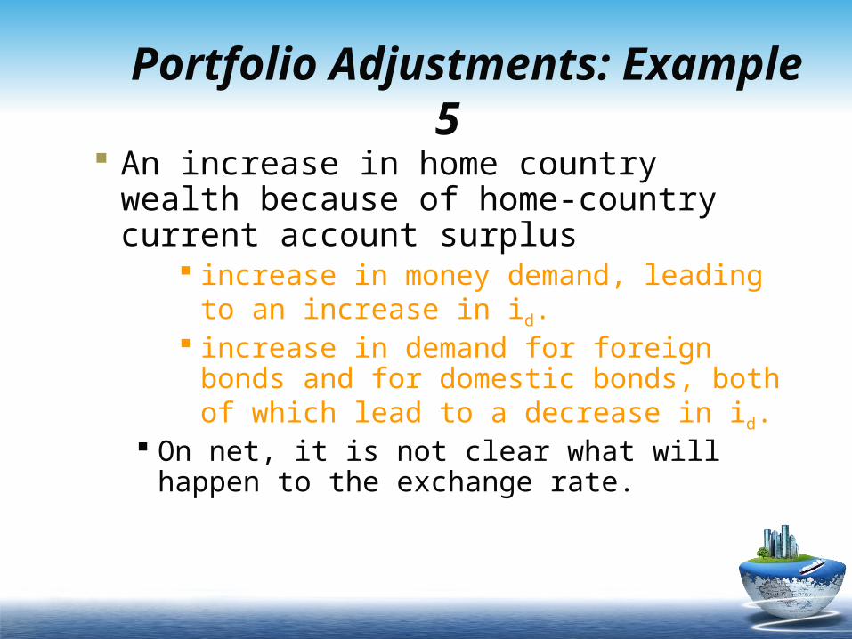
Portfolio Adjustments: Example 5
An increase in home country wealth because of home-country current account surplus
increase in money demand, leading to an increase in id.
increase in demand for foreign bonds and for domestic bonds, both of which lead to a decrease in id.
On net, it is not clear what will happen to the exchange rate.
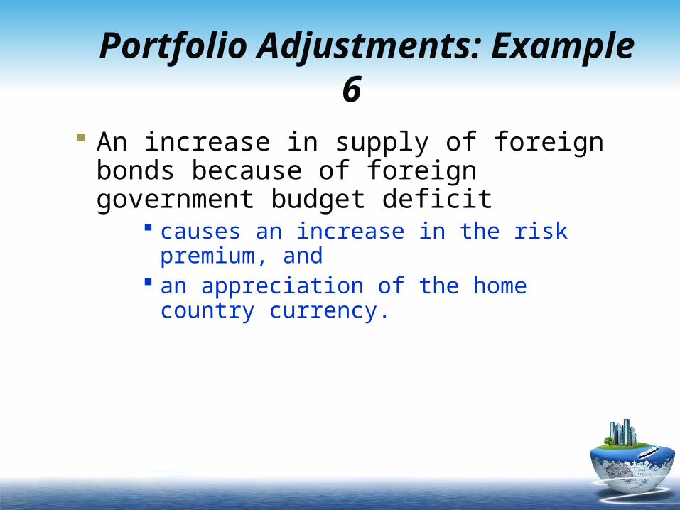
Portfolio Adjustments: Example 6
An increase in supply of foreign bonds because of foreign government budget deficit
causes an increase in the risk premium, and
an appreciation of the home country currency.
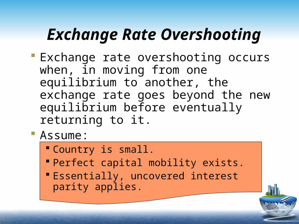
Exchange Rate Overshooting
Exchange rate overshooting occurs when, in moving from one equilibrium to another, the exchange rate goes beyond the new equilibrium before eventually returning to it.
Assume: Country is small. Perfect capital mobility exists. Essentially, uncovered interest parity
applies.
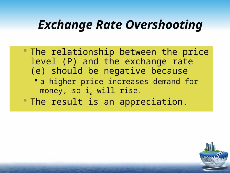
Exchange Rate Overshooting
The relationship between the price level (P) and the exchange rate (e) should be negative because a higher price increases demand for
money, so id will rise. The result is an appreciation.
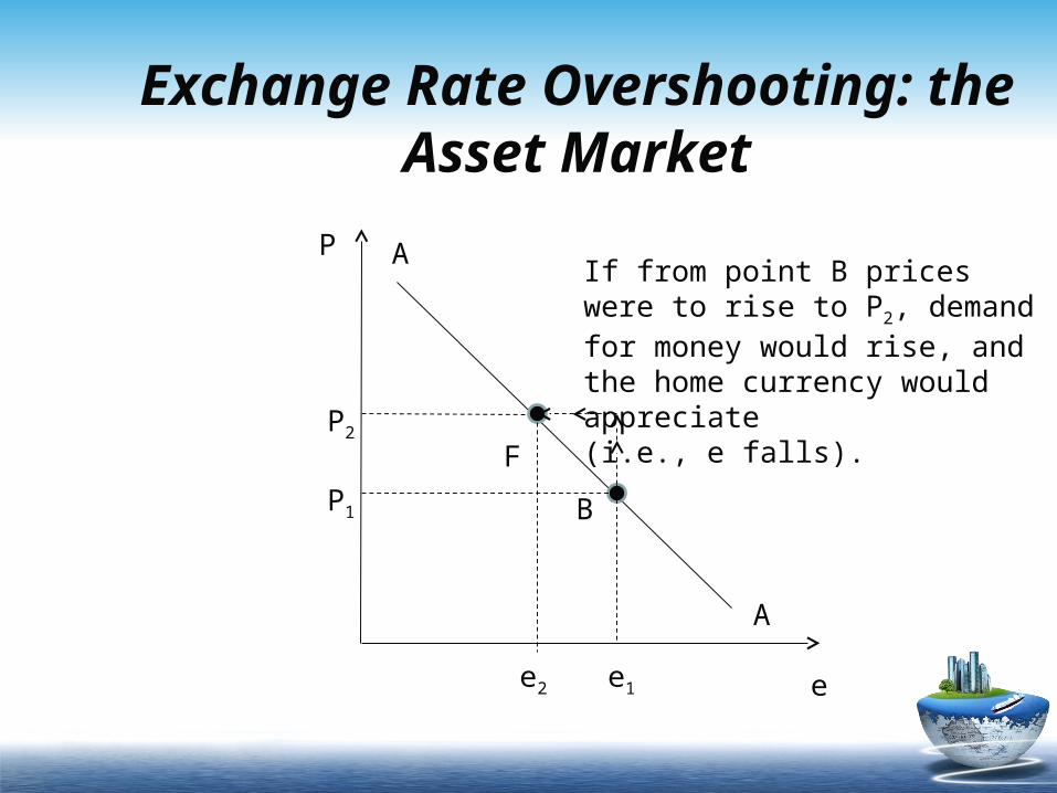
Exchange Rate Overshooting: the Asset Market
P
e
A
A
B
If from point B prices were to rise to P2, demand for money would rise, and the home currency would appreciate (i.e., e falls).
FP2
P1
e2 e1
Exchange Rate Overshooting
According to purchasing power parity, in the long run when a country’s currency depreciates its price level will increase proportionately.
That is, there is a long run positive relationship between e and P.
Let’s put this relationship together with the short run asset market relationship in a single graph.
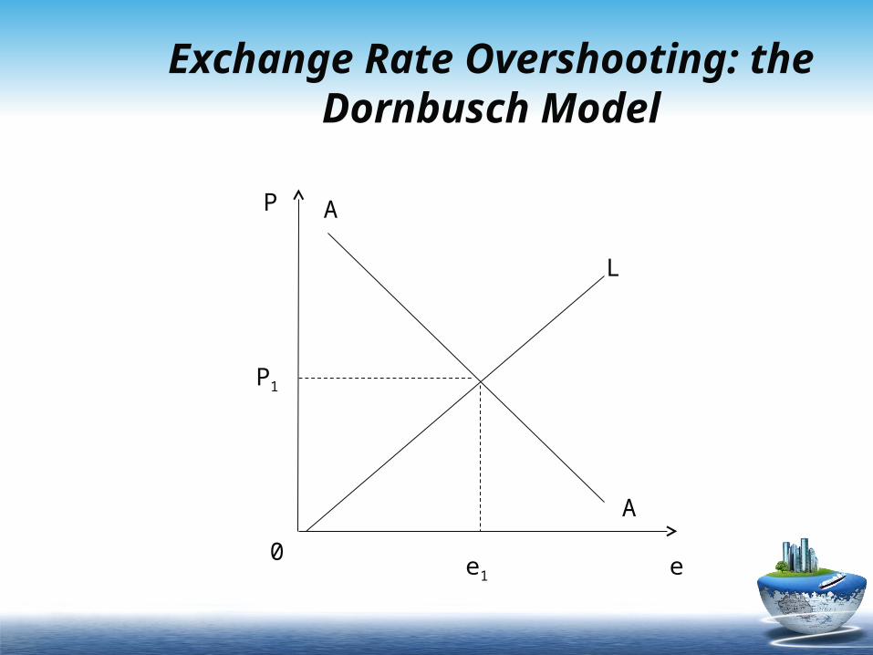
Exchange Rate Overshooting: the Dornbusch Model
P
e
A
A
P1
e1
L
0
Exchange Rate Overshooting
An increase in the money supply shifts the asset curve from AA to A'A'
This causes a relatively rapid depreciation of the home currency, from e1 to e2.
Prices eventually will begin to rise due to excess demand for goods caused by the currency depreciation.
Eventually, we reach a new equilibrium at E'
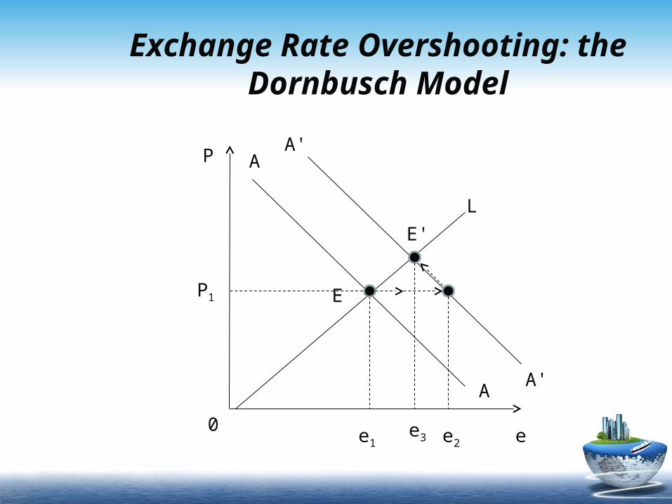
Exchange Rate Overshooting: the Dornbusch Model
P
e
A
A
P1
e1
L
0
A'
A'
E
E'
e2e3

www.themegallery.com
Add your company slogan