WritingMathematics - Birkbeck, University of London · 6 Writing Mathematics Chapter 1:...
100
Writing Mathematics Notes on L A T E X for Birkbeck Students By Sarah Hart
Transcript of WritingMathematics - Birkbeck, University of London · 6 Writing Mathematics Chapter 1:...

Writing Mathematics
Notes on LATEX for Birkbeck Students
By Sarah Hart

2 Writing Mathematics

Contents
1 Introduction 51.1 Syllabus . . . . . . . . . . . . . . . . . . . . . . . . . . . . . . . . . . . . . . . . 51.2 Learning Outcomes . . . . . . . . . . . . . . . . . . . . . . . . . . . . . . . . . . 51.3 Recommended Books . . . . . . . . . . . . . . . . . . . . . . . . . . . . . . . . . 61.4 How the software works . . . . . . . . . . . . . . . . . . . . . . . . . . . . . . . 71.5 Installing the software . . . . . . . . . . . . . . . . . . . . . . . . . . . . . . . . 71.6 Using TEXStudio . . . . . . . . . . . . . . . . . . . . . . . . . . . . . . . . . . . 81.7 Writing a simple document . . . . . . . . . . . . . . . . . . . . . . . . . . . . . . 131.8 Text, Fonts and Special Characters . . . . . . . . . . . . . . . . . . . . . . . . . 171.9 Basic Mathematics Commands . . . . . . . . . . . . . . . . . . . . . . . . . . . . 19
2 Progressing with LATEX 212.1 Lists . . . . . . . . . . . . . . . . . . . . . . . . . . . . . . . . . . . . . . . . . . 212.2 The Preamble . . . . . . . . . . . . . . . . . . . . . . . . . . . . . . . . . . . . . 242.3 Environments . . . . . . . . . . . . . . . . . . . . . . . . . . . . . . . . . . . . . 282.4 Numbering and Labelling . . . . . . . . . . . . . . . . . . . . . . . . . . . . . . . 322.5 Tables . . . . . . . . . . . . . . . . . . . . . . . . . . . . . . . . . . . . . . . . . 332.6 Other useful commands . . . . . . . . . . . . . . . . . . . . . . . . . . . . . . . . 36
3 Mathematics 373.1 Symbols . . . . . . . . . . . . . . . . . . . . . . . . . . . . . . . . . . . . . . . . 373.2 Equations . . . . . . . . . . . . . . . . . . . . . . . . . . . . . . . . . . . . . . . 433.3 Arrays and Matrices . . . . . . . . . . . . . . . . . . . . . . . . . . . . . . . . . 473.4 Figures and Diagrams . . . . . . . . . . . . . . . . . . . . . . . . . . . . . . . . 493.5 Good Mathematical Writing . . . . . . . . . . . . . . . . . . . . . . . . . . . . . 543.6 Quick Reference . . . . . . . . . . . . . . . . . . . . . . . . . . . . . . . . . . . . 56
4 Presentations 594.1 A simple presentation . . . . . . . . . . . . . . . . . . . . . . . . . . . . . . . . . 594.2 Creating a Title Page . . . . . . . . . . . . . . . . . . . . . . . . . . . . . . . . . 624.3 Themes . . . . . . . . . . . . . . . . . . . . . . . . . . . . . . . . . . . . . . . . 634.4 A Birkbeck Presentation . . . . . . . . . . . . . . . . . . . . . . . . . . . . . . . 664.5 Creating Slides . . . . . . . . . . . . . . . . . . . . . . . . . . . . . . . . . . . . 684.6 Effects . . . . . . . . . . . . . . . . . . . . . . . . . . . . . . . . . . . . . . . . . 724.7 Printing your presentation . . . . . . . . . . . . . . . . . . . . . . . . . . . . . . 76

4 Writing Mathematics CONTENTS
4.8 Ten Guidelines for a Good Presentation . . . . . . . . . . . . . . . . . . . . . . . 76
5 Dissertations 795.1 Layout of a Dissertation . . . . . . . . . . . . . . . . . . . . . . . . . . . . . . . 795.2 Choice of Document Class . . . . . . . . . . . . . . . . . . . . . . . . . . . . . . 805.3 Title Page, Abstract, Declaration . . . . . . . . . . . . . . . . . . . . . . . . . . 825.4 Table of Contents . . . . . . . . . . . . . . . . . . . . . . . . . . . . . . . . . . . 865.5 Chapters . . . . . . . . . . . . . . . . . . . . . . . . . . . . . . . . . . . . . . . . 875.6 Creating a Bibliography . . . . . . . . . . . . . . . . . . . . . . . . . . . . . . . 915.7 Using BibTeX to Manage Your Bibliography . . . . . . . . . . . . . . . . . . . . 945.8 Ten Guidelines for a Good Dissertation . . . . . . . . . . . . . . . . . . . . . . . 98

Chapter 1
Introduction
In this chapter we’ll look at how to get LATEX onto your system. We’ll give you a guided tour ofthe program TEXStudio, which is the program in which you will create documents, and whichinteracts with LATEX to produce the pdf outputs. Then we’ll go through the process of creatingbasic documents. Later chapters will look in more detail at producing mathematics, tables,figures, bibliographies, and styles of document such as presentations and dissertations. We’llbegin with the syllabus, learning outcomes and recommended resources.
1.1 Syllabus
1. Understanding the process: knowing what LATEX actually does and how to produce areadable output; producing a very simple document with basic text (assessed by Work-sheet 1)
2. Writing mathematics: how to write equations, arrays, matrices and include symbols suchas Greek letters, the symbols for the sets of integers, rational numbers and so on, integrals,sums and products (assessed by Worksheets 1 and 2)
3. Producing lists and tables (assessed by Worksheets 1 and 2)
4. Importing graphics (assessed by Worksheet 2)
5. Producing presentations: creating slides, gradual reveal and other effects (assessed byWorksheet 3)
6. Producing dissertations: title pages, chapters, tables of contents, references (assessed byWorksheet 4)
1.2 Learning Outcomes
On successful completion of this module a student will be expected to be able to:
• Be aware of some of the possible methods of producing typed mathematics, and theadvantages and disadvantages of each

6 Writing Mathematics Chapter 1: Introduction
• Be able to use simple LATEX commands, for example on Moodle discussion boards, to typeformulae
• Be able to compile documents to produce pdf outputs
• Produce different fonts and sizes of text, equations and other mathematical expressions,matrices, arrays, tables and diagrams
• Be able to label theorems, tables, figures and other items, and refer back to them bylabels
• Be able to produce a list of references and know how to cite them
• Be able to import graphics into a LATEX document
• Be able to produce: articles, presentations and dissertations in LATEX
1.3 Recommended Books
These notes aim to guide you through the process of learning LATEX. For further resources,there is a wealth of information and support at ctan.org, and in fact nearly any LATEX questioncan be answered with a quick online search. However here are three books you may considergetting.
• A Not So Short Introduction to LATEX, by Tobias Oetiker, Hubert Partl, Irene Hyna andElisabeth Schlegl. The authors have kindly made this available (free) online but it canalso be downloaded as a pdf from the Moodle page for the Writing Mathematics module.The instructions about setting things up in the first chapter are not particularly relevantto us because they are under the impression that most people use (and like) UNIX, whichis not the case! But after that it’s pretty good, with lots of examples. More detailthan you need in places though – it’s great that there is a way to produce documents inMongolian, but you may not feel you need to know that at this stage.
• Learning LATEX, by David F. Griffiths and Desmond J. Higham. SIAM, 1997. ISBN-10:0898713838, ISBN-13: 978-0898713831. This is an excellent beginners guide, coveringmost of what you need to know without any extraneous (and possibly confusing) infor-mation. It does have some omissions, for example it doesn’t cover the Beamer packagefor producing presentations, and its treatment of how to turn a .tex file into somethingreadable is a little dated. But as a concise and readable guide it does a good job.
• The LATEX Companion, by Michel Goossens and Frank Mittelbach. Addison-Wesley 2004.ISBN-10: 0201362996 ISBN-13: 978-0201362992. This book is over 1000 pages long! Itis a comprehensive guide, going far further into the gory details than is necessary for thiscourse. However some of you may like going into gory details, in which case this book isfor you.

1.4: How the software works Writing Mathematics 7
1.4 How the software works
LATEX is a very powerful typesetting system. Its aim is to present your document in a logical,aesthetically pleasing way. So if you are producing an article, there is an underlying structureof sections, subsections and numbered theorems, definitions, examples and so on within that.You can label and refer back to them in an automated way so that adding a new theorem atthe start of the article does not require you to go through renumbering all your references.
The system will arrange spacing, the size and font of text and headings, and other things,consistently according to the underlying structure. You can overrule it if necessary but usuallyyou won’t want or need to. The main reason we use it though, is because of its ability to produceprofessional-looking typeset mathematics. This is done by way of commands such as \alpha
for the Greek letter α. All this together means that when you are typing your document, it willnot look like the final pdf output. To produce the output (your completed document with allits shiny mathematics and neat layout) you need to run your file through the LATEX compiler,and out will pop a .pdf. The rough process looks like this:
• Create your document, let’s call it ‘MyFile’, with instructions for mathematics and layoutin their ‘raw’ form. You will do this in a text editor (the program TEXStudio is what wewill give you on your CD) and save it with the name MyFile.tex.
• LATEX the document (in TEXStudio this is by just clicking an icon). A .pdf| of yourdocument, called Myfile.pdf, will be produced.
And that’s basically it. I know that you may be thinking ‘but Word can do all that, whyput myself through all this pain?’ Well, Word may be able to produce some or even mostmathematics, if you push it hard enough, and if you have equation editor. But how manydrop-down menus would you need to use to create even something as simple as the expressioneiπ = −1? In LATEX you just have to type $e^i\pi = -1$. Much quicker. Perhaps moreimportant is the fact that LATEX is set up for easy cross-referencing, so you can label and referback to, for example, equations, in a way that auto-updates when you insert or remove text.There are many other advantages as well, but we’ll leave it there as I’m sure you are eager toget started. If you are in the computer room you can skip the next section about installing thesoftware, as it is already installed.
1.5 Installing the software
LATEX is free mathematical typesetting software developed over many years by the academiccommunity. There are countless forums and websites offering help and advice, and a hugearchive of resources, in particular at ctan.org. There are many free distributions of the softwareand you are welcome to explore them. However we recommend a package called ProTEXt. Thereasons for this are that it is fairly simple to install and it comes with a good, reliable andrelatively user friendly text editor (TEXStudio).

8 Writing Mathematics Chapter 1: Introduction
To install ProTEXt, go to https://www.tug.org/protext/ (or follow the link on the Moodle pagefor the module). Under the heading ‘Download and Install’, click on the phrase ‘download theself-extracting protext.exe file’. This sends you to a page that looks like this:
Now just click on protext.exe to download. It’s a large file — based on current UK averagebroadband download speed, it will take between 1 and 2 minutes to download. When you’vedownloaded it, simply run it and it will start the installation process. The download comeswith full details of how to install the software, and it is short and friendly. But basically youhave to first install MiKTEX and then TEXStudio, via a few simple steps through which themanual will guide you. It is not a gigantic program, so shouldn’t take up too much of yourworking memory. And the files you create will be small too.
If you have any difficulties installing the software itself (rather than using it), please contactNigel Foster ([email protected]) or Awuku Danso ([email protected]). They are the Depart-ment’s IT officers.
1.6 Using TEXStudio
In this section I will describe how to use TEXStudio, as this is what we are giving you to installat home. However in the 7th floor computer lab at Birkbeck there is also a program calledWinEdt, which basically does the same job; some people prefer it, so it’s up to you. There arenumerous other distributions and software that you can experiment with if you feel so inclined.
Let us assume that you have successfully installed ProTEXt on your computer, or that you arein the computer lab. Then there should be an icon on the desktop like this.
←− Double click on this icon!
You’ll see a screen with a menu bar across the top. In the top left corner click on ‘File’, then
‘New’, or just below that click on the ‘new file’ icon
. On the next page is a screenshot of

1.6: Using TEXStudio Writing Mathematics 9
what TEXStudio will look like when you have done this.
You’ll see a sidebar called ‘Structure’. This lists all the chapters, sections and subsectionsof your document. While this may be useful for longer documents, we don’t need it for ourlittle experiment, so if you like you can get rid of it by pressing the × on that sidebar. You
can bring it back by clicking on the icon at the extreme bottom left hand corner of the page.
Having got rid of the Structure sidebar, you will see that you have a blank document, called‘untitled’, and a number 1. This is line 1. Type something, such as ‘Hello World’. Now let’ssave this amazing document. Either click ‘File’, then ‘Save As’, or click the icon on the menu
bar
, and at the prompt save it as myfile. It will automatically be saved as myfile.tex
unless you specify otherwise. (You can save in any folder you like. I suggest if you are athome that you create a folder on your computer for all your LATEX documents; at Birkbeck filesshould saved either to a USB stick or your N drive.)
The name of the document you are working on will now be displayed on a tab at the top ofthe document. You can have several documents open at once, and clicking on these tabs allowsyou to move between them.

10 Writing Mathematics Chapter 1: Introduction
At this point you are ready to try compiling (or sometimes we say LATEXing or TEXing) your
document. To do this you’ll use the single green ‘compile’ arrow
. Click on it.
Oh no! Something terrible has gone wrong! Immediately some error messages will appear inthe error bar at the bottom of your screen. When you are working on documents you willregularly make errors, especially at first, and the system will let you know of these and tellyou where in the document it thinks the problem is. That’s why all the lines are numbered.Our document is currently only one line long, but you can imagine with a document of severalhundred or thousand lines, that this would be a very useful function.
OK so what has gone wrong? The error log tells us that there is an error on line 1. Wedidn’t type \begindocument. This was so cataclysmic an error that TEXStudio performedan Emergency stop. What we need to do at this point is correct any errors before attemptingto compile again.
In LATEX, some initial information is required. This is because LATEX sets up a document dif-ferently according to what it is. A book has chapters, an article doesn’t. A presentation hasslides, and a landscape page format. So we must specify which of these we are producing.The set-up of a document is called the preamble. It must include, at minimum, an instructiongiving the class of document. The simplest of these is the article class. Later we can add othercommands to the preamble. To signal that the preamble is finished we need to formally begin(and end) the document.
So, type the following four lines.
\documentclass[a4paper,12pt]article
\begindocument
Hello World
\enddocument
Here we have specified that the document is an article to be set in 12 point font on A4 pa-per. You’ll find that TEXStudio is keen to help! When you start typing commands it auto-suggests what you might want, and when you type \begindocument, it helpfully suppliesthe \enddocument for you. Which is nice.
Now we can compile our document again. Press the green arrow
. If you have typed thecommands correctly, then the error bar will present you with the happy news that the process‘exited normally’, which means that a pdf has been created that you can now look at. This
is done by pressing the ‘view’ button
, which is immediately to the right of the ‘compile’button. If you are feeling brave, and don’t expect any errors, you can compile and view all in
one go by pressing the double green arrow ‘build and view’
instead of the compile arrow.That’s what you’ll probably do most of the time.

1.6: Using TEXStudio Writing Mathematics 11
Whichever way you do it, the screen will now subdivide and you’ll see the pdf of your document(which will be called myfile.pdf) on the right hand side of the screen. Well done, you havenow produced your first LATEX document!
In the rest of this section I will briefly describe a few of the features of TEXStudio. As everwith new software, the best way in general to learn to use it is to just play with it, pressingbuttons to see what they do, hovering over buttons to get more information, and so on.The top bar looks like this. (I’ve omitted the symbols at the far right, which are to do withediting tables. We may mention them later; I never use them anyway.)
File
This menu tab allows you to create new files, open existing files and save files. One usefulfeature here is ‘New from Template’. You can select from various standard document typesand you’ll be given a document with the bare bones of what you need. So it will have a\documentclass command, for example. You can also create, open, close and save filesusing the buttons just below the File tab. Note: the ‘Print’ command here will print the .tex
file and not the pdf.
Exercise 1. Create and compile a new document called exercise1.tex containing the text‘This is some text.’
Edit
This menu tab has all the usual editing tools: undo, redo, copy, cut, paste, find and replace.Buttons for some of these also appear in the editing toolbar immediately underneath.
Idefix
The only things you are likely to use in this drop-down menu are the ‘comment’ and ‘uncom-ment’ options. If you select some text in your document that you think you may not need butdon’t want to permanently delete, you can ‘comment it out’, meaning that it stays in the filebut doesn’t appear in the pdf. You can accomplish this manually by putting a % sign beforeanything that you don’t want to be processed by LATEX. And of course here you can insertcomments for yourself. They could be reminders like %insert more on this topic here %.
Tools
LATEX does not detect spelling errors! So you are strongly advised to run a spellcheck as afinal stage in the preparation of any document. To do this you can hit the ‘Check Spelling’option in the Tools drop-down menu. You can also do a word count which ignores commands

12 Writing Mathematics Chapter 1: Introduction
as obviously they don’t contribute to the word count of your final pdf document. This is the‘Analyse Text’ option. It is in fact much more powerful than a word count but you can get oneout of it by counting all phrases containing one word.
Exercise 2. Add a deliberately misspelled word to exercise1.tex. Now run a spellcheck tocorrect it.
LaTeX and ‘Math’
These two drop-down menus have many shortcuts and aides-memoires for common commands.They are useful if you’ve forgotten (or never knew!) a particular command. But they will slowyou down a lot if you use them all the time rather than learning things. TEXStudio alreadyfinishes your commands for you so you’ll soon get the hang of it.
Vertical Toolbars
You’ll see that there are more shortcuts on the left hand side of the screen, for things likesubscripts, fractions and surds. If you bring back the ‘structure’ sidebar (by clicking on the
icon at the extreme bottom left of the screen), you’ll see another column of symbols.Clicking on these in turn brings a set of symbols that you can click on to insert the commandsfor them into your document. For example, here is what appears when you click the⇒ symbol.
All the arrows a person could wish for!
Again, it will be slow going for you if you don’t learn at least the more common of these, ratherthan finding and clicking on symbols all the time. But for symbols that you use only rarely itis a useful resource. Chapter 3 has a list of common symbols and their commands for reference.
The pdf
There are three choices for viewing your pdf. It will probably depend on the size of your screen.The default setting is that the screen will split within the window, and your pdf and .tex files

1.7: Writing a simple document Writing Mathematics 13
will appear side by side. This is the embedded viewer. The advantage of this is that you cansee everything together. The disadvantage is that you may find either your lines when typingthe .tex document are ludicrously narrow, or the writing on the pdf is too small, or both. Inthat case you may prefer to have the pdf appear in a separate window: this is the ‘windowedviewer’ option. You can switch between the embedded and windowed viewer by clicking the
icon in embedded mode to get to windowed viewer, and the
icon in windowed viewermode to get back to embedded mode. In either mode you can navigate around the pdf in theusual way, scrolling, using the up/down arrows on the keyboard or even the navigation buttonsat the top of the screen.
One extremely useful feature in the embedded and windowed viewer modes is the so-called‘inverse search’ feature. If you are looking at the pdf and you see something that needs cor-recting, if you hold down the Ctrl key and then left click, you will be taken to the correspondingline of the .tex file.
Printing
The most reliable way to print your pdf is to click the red ‘external viewer’ icon
at the topof either the embedded or windowed viewer. This will open the pdf in your standard pdf viewer(usually Adobe Acrobat). You can then print as you normally would. Caution: you mustclose the external viewer before compiling again, or you will get an error message!
1.7 Writing a simple document
In this section we will discuss (briefly) the main types of document, look at sections, subsec-tions, paragraphs and spacing, special characters, text and fonts, titles and footnotes. Morecomplicated things like drawing tables and cross-referencing are dealt with in Chapter 2. We’llalso give a very brief mention to mathematics, though that is the subject of Chapter 3.
Three Types of Document
The main three kinds of document you will need to prepare are short documents (for solutionsto coursework, Worksheets 1 and 2, the Spring progress report for your dissertation, drafts orsummaries of dissertation chapters and similar), presentations (if nothing else, for your finalproject presentation) and of course book-style longer documents, such as your dissertation.
• For short documents use the article document class.
• For presentations use the beamer document class
• For your dissertation we have prepared a special Birkbeck dissertation document class.This is the subject of Chapter 5.
Certain commands may have different effects in different classes. For example the first sectionin an article will be numbered Section 1. But sections in a book are labelled by chapter, so

14 Writing Mathematics Chapter 1: Introduction
Section 1.1 and so on. Where differences occur we will try to mention them. The defaultassumption in Chapters 1 – 3 is that we are in the article class. Anything with chapters wewill refer to as a ‘book’.
In the preamble, the first line is always to specify the document class. For example, an articlewould begin with the following command.
\documentclass[12pt,a4paper]article
The optional arguments in the square brackets can specify the font and paper size. The al-lowed font sizes are 10pt, 11pt and 12pt. If you don’t specify then you get 10pt font. For apresentation we would type the following.
\documentclassbeamer
More on those in Chapter 4.
Sections
Articles (and chapters of books) can be divided into Sections, Subsections and Subsubsections.Anything which is numbered automatically, such as theorems, will be numbered by section foran article, and by chapter for a book. You can change this default setting if you wish, in thepreamble. More on this later. To start a new section, simply type
\sectionName of Section
So, in these notes, for example, there is a line \sectionWriting a simple document. Thenumbering (in this case 1.4) is done automatically. You can produce a heading of the same sizeand typeface, but no numbering, by inserting an asterisk.
\section*Name of Section
This would produce a non-numbered section heading. There are also further subdivisions, viathe subsection and subsubsection commands.
\subsectionName of Subsection
\subsubsectionName of Subsubsection
These give numbered subsections and subsubsections. For non-numbered versions insert anasterisk. I find non-numbered subsections are useful because my sections and subsections aregenerally short enough to be easily navigable. If your sections are 15 pages long then you mightvery well want to have numbered subsections. This current subsection’s header was producedusing the command \subsection*Sections.
Exercise 3. Go to your document exercise1.tex.

1.7: Writing a simple document Writing Mathematics 15
1. Create numbered sections, subsections and subsubsections as required, so that the docu-ment has subdivisions labelled 1 Introduction, 1.1 Definitions, 1.2 Results, 1.2.1Theorems, and 1.2.2 Corollaries.
2. Add a new numbered section calledPreliminaries, before Introduction. What happensto the numbering – what number, for example, is the Corollaries section now given?
3. What happens if you put a subsection right at the beginning of the document before youhave started a section?
Paragraphs and Spacing
If you leave a blank line in your .tex file, then LATEX will start a new paragraph, with automaticindentation at the start. (Actually I don’t really like indented paragraphs so I put the command\parindent 0pt in my preamble.) If you want to leave a blank line in the text you create,you’ll need to leave a blank line and type \\ and the end of the previous line. You can leavesmall, medium or large gaps by using the \smallskip, \medskip and \bigskip commands.Below you see the effect of these commands.
The line ends here.
After this line I put a double backslash.
Here follows a small gap.
Here follows a medium one.
And here’s a big one.
The commands that produced the above sequence of lines and spaces are as follows.
The line ends here.
After this line I put a double backslash.\\
Here follows a small gap.\smallskip\\
Here follows a medium one.\medskip\\
And here’s a big one.\bigskip\\
You can get an arbitrary vertical space with (for example) \vspace1cm. You can get a hori-zontal space with (for example) \hspace1cm. If you wish to write text right at the end of theline, then you can use the \hfill command (similarly \vfill puts text at the bottom of thepage). So the command left \hspace5cm middle \hfill right produces the followingoutput text.
left middle right
16 Writing Mathematics Chapter 1: Introduction
Note Sometimes you may wish to give a paragraph a title (this paragraph is called Note asan example). This was done using the command \paragraphNote, and then writing the textas normal.
It is possible to centre-justify a portion of text by typing \begincenter at the start and\endcenter at the end. This is called centering; I’m afraid you do have to use the
American spelling.
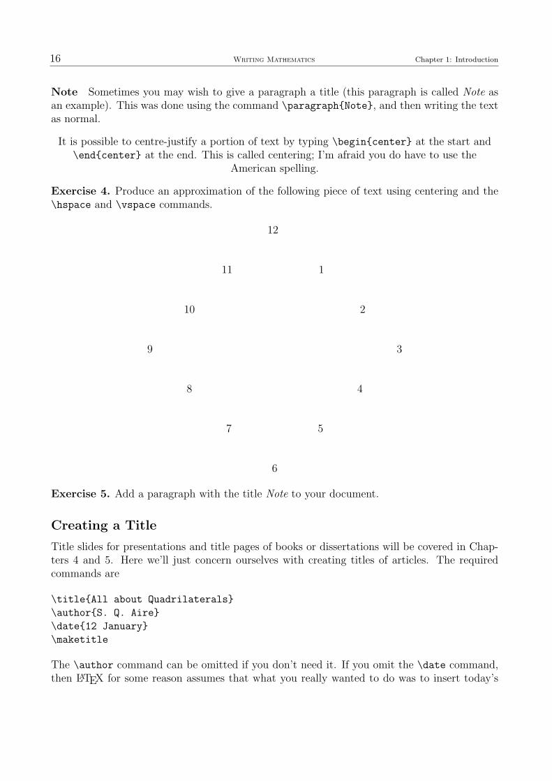
Exercise 4. Produce an approximation of the following piece of text using centering and the\hspace and \vspace commands.
12
11 1
10 2
9 3
8 4
7 5
6
Exercise 5. Add a paragraph with the title Note to your document.
Creating a Title
Title slides for presentations and title pages of books or dissertations will be covered in Chap-ters 4 and 5. Here we’ll just concern ourselves with creating titles of articles. The requiredcommands are
\titleAll about Quadrilaterals
\authorS. Q. Aire
\date12 January
\maketitle
The \author command can be omitted if you don’t need it. If you omit the \date command,then LATEX for some reason assumes that what you really wanted to do was to insert today’s

1.8: Text, Fonts and Special Characters Writing Mathematics 17
date, so it does that! If you want to omit the date, then you need to type \date. Theremay be occasions when you feel a ‘formal’ title takes up too much room on the page, perhapsif your document is only a page long, for example, and/or doesn’t need to give author and/ordate. In this case I recommend creating something manually like the following.
\begincenter\Large All about Quadrilaterals\\
S. Q. Aire
\endcenter
Exercise 6. Open your document exercise1.tex (or start a new one).
• Give your document a title, author and date.
• Now remove the date from the title.
• Give it a date but no author.
• Now manually create a title.
1.8 Text, Fonts and Special Characters
Special Characters
The following characters have a special meaning in LATEX.
\ & $ % ∼ _ # ^
I won’t go into all of them just now, though we have already encountered the backslash (\),because it precedes every command. To get a backslash in text, you must type $\backslash$.A forward slash, /, has no special role so you can just type it as normal. All the special charac-ters other than the backslash can be obtained by typing a backslash before them. So \& givesyou &, \% gives you %, and so on. It’s quite common to forget that % is a special character. Ifyou do this then you’ll find a chunk of text missing because, if you remember, the special roleof the % sign is to comment out any text that follows it.
I’ll mention hyphens here too. There are three lengths possible. The short one, which is justthe standard hyphen on the keyboard, should be used when hyphenating a word, such as ‘do-gooder’. The second is a dash, obtained by typing two hyphens (--), which is used when youtype something like May – June. There is also a long dash, which is three hyphens together —it is probably the one you will use least.
Exercise 7. In your document exercise1.tex or elsewhere, reproduce the following output.
The national debt of the USA is approximately $16 trillion. It is about 73% of GDP.The USA’s credit rating was downgraded in 2011 by the credit ratings agency Standard &Poor’s.

18 Writing Mathematics Chapter 1: Introduction
Text and Fonts
The size of body text is determined by the optional argument to the \documentclass commandat the beginning of the preamble. You can specify 10pt, 11pt or 12pt, as we’ve mentioned. Thedefault is 10pt. Parts of your text can be made tiny, footnote size, small, normal, large, Large
to huge. You can use bold type. You can also emphasise words. Then we have italic type,slanted type and small caps type. The last two sentences were produced as follows.
Parts of your text can be made \tiny tiny, \footnotesize footnote size,
\small small, normal, \large large, \Large Large to \huge huge. You
can use \bf bold type. You can also \em emphasise words. Then we have
\it italic type, \sl slanted type and \sc small caps type.
The \em command is the best if you want to italicise something. The reason is that LATEX isintelligent with this command. If you are in normal text, then the result of this command wouldproduce something like this. But if you emphasise something while you are already writing initalics, such as a quotation or the statement of a theorem, the command would reflect that.Thus, for example, consider the text, ‘\it Do you expect me to \em talk?’ ‘No, Mr
Bond, I expect you to \em die.’ This produces: ‘Do you expect me to talk?’ ‘No,Mr Bond, I expect you to die.’ Note the different symbols required to produce left and rightquotation marks. For a left quotation mark you need the left dash (usually located on thekey to the left of the 1 on a keyboard). For a right quotation mark you need the standardapostrophe. Finally the command for LATEX is \LaTeX.
Exercise 8. Reproduce the following paragraph of text. (Don’t worry if your lines are not thesame length, and certainly don’t try to get a box round it – I’m just interested in the actualwords being reproduced in the same typefaces.)
Very soon the Rabbit noticed Alice, as she went hunting about, and called out to herin an angry tone, ‘Why, Mary Ann, what are you doing out here? Run home this moment,and fetch me a pair of gloves and a fan! Quick, now!’ And Alice was so much frightenedthat she ran off at once in the direction it pointed to, without trying to explain the mistakeit had made. She came upon a neat little house, on the door of which was a bright brassplate with the name ‘W. Rabbit’ engraved upon it.
Accents
If you are using non-English words then you may need accents. Your encyclopædic knowledgeof mathematicians like Godel, Erdos and L’Hôpital may require it. (That sentence was broughtto you by the following raw text: encyclop\aedic knowledge of mathematicians like
G\"odel, Erd\Hos and L’H\^opital). Because these commands are used rarely, evenan old hand like me cannot necessarily remember them all. This is one instance where it isprobably quicker to use one of the side menus. In TEXStudio, bring up the left vertical sidebar
(if necessary by clicking on the icon at the extreme bottom left of the screen). Now click on

1.9: Basic Mathematics Commands Writing Mathematics 19
the á symbol. You’ll see a full range of accented letters to choose from. When you want one,just click on it and the command will appear in your text. The following table lists just someof the more commonly required accented letters and their corresponding LATEX commands.
Accented Letter Commande \"e
é \’e
è \‘e
c \cc
à \‘a
o \"o
ô \^o
œ \oe
Sometimes an accent isn’t in the list. In the next exercise there is a Vietnamese accent required(ả). When I was writing the exercise I went looking for mathematicians whose names haveaccented letters, and in the list of Fields medal winners the three in the exercise cropped up.Rather than not include this unusual accent, I decided that it was a good example of how easyit is to find out how to do things, and an example of the kinds of instructions that are putin the preamble to a document (Section 2.2 has much more on this). I Googled ‘Vietnameseaccents latex’; the first hit told me exactly how to add required characters.
Exercise 9. Open your document exercise1.tex (or start a new one). In the preamble (thepart before \begindocument), add the line \usepackage[T1,T5]fontenc. This allows youto use many more accented letters. In particular, the Vietnamese letter ả is obtained by typing\h a. Now reproduce the following output. (Make sure you get those hyphen lengths right!)
The name Gauss — if you want to show off — could more correctly be written Gauß. Themathematicans René Thom, Lars Hormander and Ngô Bảo Châu have all won the Fieldsmedal.
1.9 Basic Mathematics Commands
The whole of Chapter 3 of these notes is devoted to mathematics, and so I won’t say muchhere. But I did want to at least give you the absolute basics so that you can experiment a littleat this point. The first and most important thing to learn is that any mathematics should beenclosed in dollar signs. And I mean any mathematics. Look at the difference between typing10-3=7 and $10-3=7$. The first gives 10-3=7 and the second gives 10−3 = 7 (note the properlength minus sign and better spacing). Moreover when you are referring to, say, a group G or areal number x, these are mathematical terms which are usually italicized. So those two shouldbe contained in dollar signs (so we write $G$ and $x$). If you neglect to do this then you endup with a group G and a real number x. The x in particular looks ugly and not how we wantto write variables. If you want to display mathematics in a centred line, then instead of onedollar sign, you should use two. For example, writing $$10-3=7$$ produces
10− 3 = 7.
20 Writing Mathematics Chapter 1: Introduction
Be careful! If you are finishing a sentence with your displayed equation, you need to put thefull stop inside the dollar signs with the equation. Otherwise it will just end up at the startof the next line of text, which looks silly. Equations can be numbered, and we will give moredetail about that in Chapter 3.
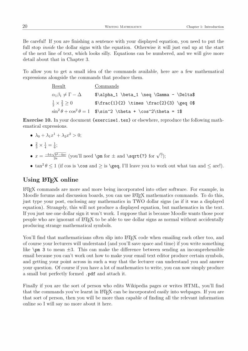
To allow you to get a small idea of the commands available, here are a few mathematicalexpressions alongside the commands that produce them.
Result Commands
α1β1 6= Γ−∆ $\alpha_1 \beta_1 \neq \Gamma - \Delta$
12× 2
3≥ 0 $\frac12 \times \frac23 \geq 0$
sin2 θ + cos2 θ = 1 $\sin^2 \theta + \cos^2\theta = 1$
Exercise 10. In your document exercise1.tex or elsewhere, reproduce the following math-ematical expressions.
• λ0 + λ1x1 + λ2x
2 > 0;
• 23× 1
4= 1
6;
• x = −b±√b2−4ac2a
(you’ll need \pm for ± and \sqrt? for√
?);
• tan2 θ ≤ 1 (if cos is \cos and ≥ is \geq, I’ll leave you to work out what tan and ≤ are!).
Using LATEX online
LATEX commands are more and more being incorporated into other software. For example, inMoodle forums and discussion boards, you can use LATEX mathematics commands. To do this,just type your post, enclosing any mathematics in TWO dollar signs (as if it was a displayedequation). Strangely, this will not produce a displayed equation, but mathematics in the text.If you just use one dollar sign it won’t work. I suppose that is because Moodle wants those poorpeople who are ignorant of LATEX to be able to use dollar signs as normal without accidentallyproducing strange mathematical symbols.
You’ll find that mathematicians often slip into LATEX code when emailing each other too, andof course your lecturers will understand (and you’ll save space and time) if you write somethinglike \pm 3 to mean ±3. This can make the difference between sending an incomprehensibleemail because you can’t work out how to make your email text editor produce certain symbols,and getting your point across in such a way that the lecturer can understand you and answeryour question. Of course if you have a lot of mathematics to write, you can now simply producea small but perfectly formed .pdf and attach it.
Finally if you are the sort of person who edits Wikipedia pages or writes HTML, you’ll findthat the commands you’ve learnt in LATEX can be incorporated easily into webpages. If you arethat sort of person, then you will be more than capable of finding all the relevant informationonline so I will say no more about it here.

Chapter 2
Progressing with LATEX
In this chapter we will cover some more advanced topics, including lists, construction of ta-bles, the preamble, numbering and labels (for cross-referencing), environments and other usefulcommands. Environments are things like theorems, examples and definitions. By the end ofthe chapter you should be able to produce more or less all of the text formatting, layout andstructure that you need. Formatting of mathematics is left for Chapter 3.
2.1 Lists
In this section we will look at lists. There are various kinds of lists, both numbered andun-numbered, that can be created. LATEX will automatically keep count and nest lists sys-tematically. So, for example, we could have the following set-up, which is started with thecommand \beginenumerate.
1. The top numbering is with arabic numerals 1, 2, 3. (one can change this but that’s a bitmore advanced).
2. Each item in the list is preceded by the command \item.
(a) The next level is letters, so we get (a)
(b) followed by (b).
i. After that it’s Roman numerals.
ii. If you are using this many sub-lists, maybe it’s time to organise your thoughtsmore clearly!
(c) Don’t forget you need to type \endenumerate at the end of each list, so here Ihave had to type it 3 times in total.
3. I think that’s enough enumerated lists.

22 Writing Mathematics Chapter 2: Progressing with LATEX
The commands on the left below generate the text on the right.
\beginenumerate
\item Vertebrates 1. Vertebrates\beginenumerate
\item Birds (a) Birds\beginenumerate
\item Penguins (i) Penguins\endenumerate
\endenumerate
\endenumerate
If you want bullets, then you use the itemize command.
• Bullet points are not used very much in mathematical writing.
• But on occasion they can be useful.
• When giving a project presentation, short bullet points are better than acres of text.
The following commands illustrate what happens when we use itemize instead of enumerate.
\beginitemize
\item Vertebrates • Vertebrates\beginitemize
\item Birds – Birds\beginitemize
\item Penguins ∗ Penguins\enditemize
\enditemize
\enditemize
The final type of list I will mention is a catch-all set-up which allows you to specify what theitems in a list will be labelled; it is the trivlist command. Here is an example: A group isa non-empty set, G, together with a map ∗ defined on G×G, satisfying four axioms G0 – G3.
G0 (closure) For all g, h ∈ G, g ∗ h ∈ G.
G1 (associativity) For all g, h, k ∈ G, (g ∗ h) ∗ k = g ∗ (h ∗ k).
G2 (identity) There is an element e ∈ G, such that for all g ∈ G, g ∗ e = e ∗ g = g.
G3 (inverses) For all g ∈ G, there is an element g−1 ∈ G, such that g ∗ g−1 = e = g−1 ∗ g.
This is produced with the following commands in the .tex file.

2.1: Lists Writing Mathematics 23
\begintrivlist
\item[\bf G0] \bf (closure) For all $g, h \in G, g \ast h \in G$.
\item[\bf G1] \bf (associativity) For all $g, h, k \in G$, $(g \ast h)
\ast k = g \ast (h \ast k)$.
\item[\bf G2] \bf (identity) There is an element $e \in G$, such
that for all $g \in G$, $g \ast e = e \ast g = g$.
\item[\bf G3] \bf (inverses) For all $g \in G$, there is an element
$g^-1 \in G$, such that $g\ast g^-1 = e = g^-1 \ast g$.
\endtrivlist
Exercise 11. Reproduce the following text. (You’ll need \dot9 for 9).
Equivalent expressions.
1. (a) 0.5
(b) 12
(c) 0.49
2. 8 o’clock in the evening can be written as:
(a) 8 pm
(b) 2000h
(c) 20:00
Exercise 12. Reproduce the following text. You’ll need a couple of mathematical symbols, ≡($\equiv$) and mod n ($\modn$).
Method for solving a linear congruence ax+ b ≡ c mod n.
• Subtract b from both sides to get Ax ≡ B mod n.
– If gcd(A, n) does not divide B, then there are no solutions. STOP.
– If gcd(A, n) divides B then there are solutions. Continue to next step.
• Divide A, B and n by gcd(A, n) to get a congruence kx ≡ l mod m for appropriatek, l,m.
• Reverse the Euclidean algorithm to find u, v with uk + vm = 1.
• Then x ≡ ul mod m is the solution to the original congruence.

24 Writing Mathematics Chapter 2: Progressing with LATEX
2.2 The Preamble
The preamble is the place for global commands. That is, instructions that affect the wholedocument. It starts of course by specifying the class of document – usually an article. Butthere are numerous other things we can include. I have described the main four in this section.Note that the first line of the preamble should always be the \documentclass command.
Packages
Part of what keeps LATEX such a tight, efficient program is that it doesn’t have extraneousfeatures that you never use. This goes back to its early days when computers had much lessmemory. However there are many functions and features that can be added simply by includingbolt-ons called packages. If you want to use a given package, you need to add an instruction tothat effect in the preamble. The software can then check that the package is installed on yourcomputer. If it isn’t, then ProTEXt can auto-install it for you.
We have already seen an example of a package in Section 1.8. Here we wanted to use a Viet-namese accented character. In the preamble we added the line
\usepackage[T1,T5]fontenc
and then when we needed the extra commands provided by the package, we could just use themas normal in the text. You are not likely to need any packages beyond the ones I suggest (andmaybe not even them!), but the format for adding them is always the same.
\usepackage[optionalargument]package name
Of course it is perfectly possible to create a complete document without using any extra pack-ages. But there are six packages I use so enough that I just insert them into every document.Usually this is by taking a document I’ve already written, saving it under the new name, thendeleting everything except the preamble.
\usepackageamssymb
\usepackageamsmath
\usepackageamsfonts
\usepackageamsthm
\usepackagegraphicx
\usepackageepstopdf
The first four of these are packages created by the American Mathematical Society. They giveextra symbols, mathematics commands, fonts and ways to format theorems. The next two areto do with incorporating graphics into your document, so can be omitted if you don’t have any.We’ll discuss graphics in more detail in Section 3.4.

2.2: The Preamble Writing Mathematics 25
Page Setup
You do not need to give any page setup commands in the preamble if you don’t want to! Forthe \documentclass[a4paper]article class the page size is obviously A4, which is a page210mm wide and 297mm high. Margins and text width are determined by giving the top mar-gin and text height, the left margin and text width.
By default the top margin is 52mm, the text height is 210 (including the page number at thebottom), meaning that the bottom margin (after the page number) is 35mm. The left marginis 39mm, the text width is 130mm, meaning that the right margin is 41mm.
Any changes you make to the top margin or left margin are in reference to these existing de-faults of 52mm for top margin and 39mm for odd side margin. My suggestion is that you tryand keep the rough proportions similar to what the clever designers of LATEX set up. So ifyou want to add 20mm to your text height, you should take off half that, namely 10mm, fromthe top margin (these two commands combined will force the loss of 10mm from the bottommargin). This is done using the \addtolength command.
\addtolength\topmargin-10mm
\addtolength\textheight20mm
There are commands which allow you to give the absolute value of the textheight, but theadvantage of \addtolength is that you don’t have to remember what the default settings were,as you are just adding and subtracting.
To change the left and right margins and the text width you need to remember that in booksusually the odd and even numbered pages are symmetrically formatted, often with a slightlywider ‘outside’ margin (the right margin on odd numbered pages and the left margin on evennumbered pages), and a slightly narrower ‘inside’ margin. The odd side margin in LATEX is theleft margin on odd numbered pages. The even side margin is the left margin on even numberedpages. So to change the left margins of your document you need to look at both of these. Thesimplest way is again probably with the \addtolength command; an example is below.
\addtolength\oddsidemargin-5mm
\addtolength\evensidemargin-5mm
\addtolength\textwidth10mm
At this point in the preamble you can also set things like the indentation on paragraphs, thedistance between paragraphs, and whether pages are numbered. If you don’t want pages tobe numbered then use the command \pagestyleempty. If you want headings automaticallyproduced by LATEX (such as the title of the document appearing on every page) then you caninclude \pagestyleheadings. More complicated instructions are not discussed here but youcan customise almost infinitely. For paragraphs if you want to change the defaults you can usethe commands

26 Writing Mathematics Chapter 2: Progressing with LATEX
\parindent 5pt (for example, this sets the indent to 5pt);\parsep 5mm (for example, this sets the gap between paragraphs to 5mm).
LATEX understands several units of measurement. Points (pt), millimetres (mm), centimetres(cm) and inches (in) are the four you are most likely to want to use.
Exercise 13. In this exercise you will be creating an article and experimenting with formatting.To see the effects you will need at least two pages of text. I suggest cutting and pasting fromsomewhere, either any old text file you have lying around, or, for example, a chunk of this text.(Don’t worry it’s just the text of Alice in Wonderland.)
http://www.gutenberg.org/cache/epub/11/pg11.txt
Create an article with at least two pages of text, satisfying the following.
• It should be 11 point font, and A4 paper.
• It should contain three numbered sections.
• The pages should be numbered and have headings.
• The text should be 30mm higher than the default setting, and the topmargin should be15mm shorter.
• The text should be 20mm wider than the default, and the left margins of both odd andeven numbered pages should be 10mm narrower than the default.
• The indentation of paragraphs should be 20mm.
Instructions about Commands
The next part of the preamble should be given over to instructions about commands. Thisis where you can modify the way LATEX processes various things like lists, theorems and soon. For example you can specify whether theorems are numbered by chapter or section. Youcan specify the numbering style of lists. Redesigning lists is not difficult but is probably notsomething you will need to do. If you do, then simply look online for \theenumi. Instructionsto do with theorems are covered in Section 2.3.
New Commands
We have already established that LATEX can do everything, so why on earth would any saneperson need new commands? Nearly always it is done to save time. For example, I have thefollowing set of new commands in my preambles.
\newcommand\zz\mathbbZ
\newcommand\qq\mathbbQ
\newcommand\rr\mathbbR
\newcommand\cc\mathbbC

2.2: The Preamble Writing Mathematics 27
This is because I use the symbols Z, Q, R and C so often that it saves me a lot of time to type$\rr$ instead of $\mathbbR$ when I want the symbol R. A colleague defines a shorter wayof beginning and ending lists.
\newcommand\be\beginenumerate
\newcommand\ee\endenumerate
Then instead of \beginenumerate he just has to type \be. Much quicker. A final exampleis that for me the default letter epsilon (given by $\epsilon$) is this: ε. But I prefer this: ε.The command for that is a bit long: $\varepsilon$. So in my preamble I have:
\newcommand\ep\varepsilon
meaning to get the symbol ε I just have to type $\ep$.
You can define as many of these commands as you like, and copy and paste them from documentto document. Sometimes you may get an error message to say that the command is alreadydefined. In that case you’ll need to give your command a different name.
Organising your Preamble
It is good practice to put all commands of a similar kind together in the preamble. This makesit easier to find where they are if you want to change them, and also easier to cut and pastwholesale when starting a new document. As an example, the preamble for a typical articlemight go like this.
\documentclass[a4paper,12pt]article
% % % % % % % % % % % % % % % % %packages
\usepackageamssymb
\usepackageamsmath
\usepackageamsfonts
\usepackageamsthm
\usepackagegraphicx
\usepackageepstopdf
% % % % % % % % % % % % % % % % %page setup
\textwidth 170mm
\oddsidemargin -5mm \evensidemargin -5mm \topmargin -5mm \textheight 227mm
% % % % % % % % % % % % % % % % %instructions
\newtheoremthmTheorem[section]
\newtheoremlemma[thm]Lemma
% % % % % % % % % % % % % % % % %new commands
\newcommand\rr\mathbbR
\newcommand\cc\mathbbC
Remember that the commands beginning \newtheorem will be discussed in Section 2.3.

28 Writing Mathematics Chapter 2: Progressing with LATEX
Exercise 14. When I am writing about linear algebra I include the following commands in mypreamble.
\newcommand\bu\mathbfu
\newcommand\bv\mathbfv
\newcommand\bw\mathbfw
\newcommand\bo\mathbf0
Add these to your preamble and then in your document use them to produce the following
output. Note that \sum_a^b produces∑b
a in a line of text andb∑a
in displayed equations.
Suppose for some ai, bj, ck we have
l∑i=1
aivi +m∑j=1
bjuj +n∑k=1
ckwk = 0.
Then∑l
i=1 aivi +∑m
j=1 bjuj =∑n
k=1(−ck)wk.
2.3 Environments
Environments are parts of the document that have different properties from normal text; theygenerally sit between commands \beginwhatever and \endwhatever. Lists are a kind ofenvironment – we have the enumerate, itemize and trivlist varieties. Tables are another environ-ment type. The center environment is very useful. Displayed equations (another environmenttype) are centre justified automatically, but we can also make text, or tables, or pictures, appearcentrally. (I’m sorry that we are forced to use American spelling, but such is life.) The command
\begincenter \em To be or not to be, that is the question.\endcenter
produces the following centred quotation.
To be or not to be, that is the question.
Next, we have arrays. These are used when in mathematics mode, such as in the case wherewe are giving different values to a function. The array environment is a kind of ‘maths mode’version of the tabular environment that is used to produce tables. The following is just anindicative example; don’t worry about the detail. Tables are dealt with properly in Section 2.5,and for arrays see Section 3.3.
A function $f: \mathbbR \rightarrow \mathbbR$ is defined as follows.
$$f(x) = \left\\beginarrayll \sqrtx & \mathrmif\; x \geq 0\\
0 & \mathrmotherwise
\endarray
\right.$$

2.3: Environments Writing Mathematics 29
These commands produce the following text.
A function f : R→ R is defined as follows.
f(x) =
√x if x ≥ 0
0 otherwise
Incidentally the \; command that you’ll see in the source file inserts space. You could also dothis with the \hspace*2mm command. Don’t worry too much about the other commands; asI’ve said these will be discussed in the relevant sections later.
I suppose I should mention that the way I’m getting all this text that looks like typing is withthe verbatim environment. Anything typed in this environment comes out exactly as it istyped, with no LATEXing applied. But I don’t suppose you’ll need it.
Finally we have the theorem environment. This is the environment that covers theorems,lemmas, propositions, corollaries, definitions and anything else that needs numbering. If yourdocument needs any or all of these, you will need to set up these environments in the preamble.You should use the amsthm package by inserting the command \usepackageamsthm in thepreamble.
For each object you wish to define you need a line in the preamble.
\newtheoremnameoutput[number by]
The name is how you will signify this type of theorem in the raw text. The output is how it willbe labelled in the output pdf. The optional [number by] argument tells LATEX how you wouldlike to number this object – by section, by chapter, and so on. Let’s see an example. Everydocument needs theorems. So we put a line in the preamble specifying what our theorems willbe named.
\newtheoremthmTheorem[section]
Then to put a theorem in the text we type:
\beginthm
Some text.
\endthm
This will result (supposing it is the first theorem in Section 1 of an article) in the followingoutput.
Theorem 1.1. Some text.

30 Writing Mathematics Chapter 2: Progressing with LATEX
In the preamble to the document, if you want lemmas, propositions and so on, you’ll need toset them up individually so that they are numbered as you wish. Some people want all resultsto be numbered in sequence Theorem 1, Proposition 2, Example 3, and so on, but others preferindependent numbering: Theorem 1, Proposition 1, Example 1. You can have your objectsnumbered by chapter, section or even subsection.
For example, in the preamble of this document is a line setting up a Lemma environment.\newtheoremlemma[thm]Lemma
This creates a theorem environment, started by \beginlemma and ended by \endlemma,that is numbered with Theorems and named ‘Lemma’. Looking below we see that Lemma 2.2is numbered as a theorem. If instead we had written \newtheoremlemmaLemma[section],this would change.
Theorem 2.1. Any group of prime order is simple.
Lemma 2.2. Every group of order 15 is cyclic.
Usually we want theorems, lemmas and so on to be formatted as you have seen above; thatis, labelled in bold font and with the text in italics. But there are other objects such as def-initions, that we may not wish to italicise. To cater for these the package amsthm has three‘styles’ of theorem-type object. These are plain, definition and remark. The default settingis theorem. To see the difference in formats, suppose we define a new theorem environmentcalled Conjecture. We write the following in the preamble.
\theoremstylestyle
\newtheoremconjectureConjecture[section]
Here style is one of plain, definition or remark. If no style is specified then the default isplain. To put a conjecture in the text, we would type the following.
\beginconjecture
This is some text.
\endconjecture
The effect of the different styles on the output is shown below. (I’ve assumed this is an articleand this is the first conjecture in Section 1.)
plain Conjecture 1.1. This is some text.definition Conjecture 1.1. This is some text.remark Conjecture 1.1. This is some text
Note that the theorem style is either the default or the last style specified; you don’t have torestate it for every \newtheorem. As a guide, I have the following lines included in the preamblefor most of my documents.

2.3: Environments Writing Mathematics 31
\usepackageamsthm
%
\theoremstyleplain
\newtheoremthmTheorem[section]
\newtheoremconjecture[thm]Conjecture
\newtheoremcor[thm]Corollary
\newtheoremlemma[thm]Lemma
\newtheoremprop[thm]Proposition
%
\theoremstyledefinition
\newtheoremexample[thm]Example
\newtheoremdefn[thm]Definition
Where there are theorems, there are proofs. The amsthm package has a proof environment. Inthe text you can then type the following.
\beginproof
The proof is an exercise for the reader. \endproof
This will produce:
Proof. The proof is an exercise for the reader.
Sometimes the proof of a result is not immediately underneath the statement of that result.In those circumstances it is good form to specify what you are proving. This can be doneby inserting an optional argument in square brackets. So for example if there has been somediscussion of ancient Greek mathematics following a statement of Pythagoras’ Theorem, thenwhen it is time to give the proof, instead of \beginproof, we could type:
\beginproof[Proof of Pythagoras’ Theorem]
This is the outcome.
Proof of Pythagoras’ Theorem. Insert your favourite proof here.
Incidentally if the last line of your proof is a displayed equation then unless you tell it otherwise,LATEX will stupidly put the QED symbol (a square) on an empty line underneath the equation.To avoid this just type \qedhere at the end of the equation. Then finish the equation (that is,put the two dollar signs) and type \endproof as normal.
Exercise 15. Create a document with two sections. Set up lemmas, propositions, theoremsand corollaries in your preamble in such a way that your document contains the following items.
• Lemma 1.1. The following holds: 1 + 1 = 2.
• Proposition 1.2. The following holds: 2 + 1 = 3.
• Theorem 2.1. The following holds: 3 + 1 = 3.

32 Writing Mathematics Chapter 2: Progressing with LATEX
• Corollary 2.2. The following holds: 2 + 2 = 4.
Then include a proof of Corollary 2.2.
Exercise 16. 1. Alter your preamble commands in Exercise 15 such that your documentinstead contains the following items.
• Lemma 1.1. The following holds: 1 + 1 = 2.
• Proposition 1.1. The following holds: 2 + 1 = 3.
• Theorem 2.1. The following holds: 3 + 1 = 3.
• Corollary 2.2. The following holds: 2 + 2 = 4.
2. Alter your preamble commands again so that now the items are labelled as follows.
• Lemma 1. The following holds: 1 + 1 = 2.
• Proposition 2. The following holds: 2 + 1 = 3.
• Theorem 3. The following holds: 3 + 1 = 3.
• Corollary 1. The following holds: 2 + 2 = 4.
2.4 Numbering and Labelling
LATEX, as we have seen, produces a structure which can include numbered chapters (in thecase of a book), sections, subsections and so on. It can also number tables, figures, theorems,examples, exercises, equations and many other things. Anything that is numbered by LATEXcan be labelled in the .tex file to allow automatic cross-referencing. This is an extremely usefuland important tool. It allows you to make changes to your document without worrying thatyou’ll need to go through and check that all the numbers are still right. So you can insert anew section, which will cause all subsequent sections to be renumbered, and if you have cross-referenced using your labels then these cross-references will be automatically updated.
To label something, use the \label command. So to start this section I typed the following.
\sectionNumbering and Labelling\labelnumbering
Now I can refer to it in the text by typing, for example,This is Section \refnumbering.
That produces the output, ‘this is Section 2.4’. There is no need to label everything, by the way,only things you are going to need to refer back to. But if you are going to refer to somethingyou should always use the \label and \ref commands because then you are protectedagainst your unexpected future decisions to add or remove things at the last minute.
The most likely objects to be cross-referenced are theorems, definitions and similar things. Tolabel them simply insert \labelmyresult (or similar) after \beginlemma (and obviously
2.5: Tables Writing Mathematics 33
before \endlemma). Then to refer back to this lemma type ‘by Lemma \refmyresult . . . ’.
Tables and Figures are environments that produced numbered Tables and Figures that cantherefore can be labelled and cross-referenced. We haven’t dealt with those environments yet(see Sections 2.5 and 3.4 for more information), but broadly speaking, the approach is thesame as for the theorem environment – insert a \label command and then cross-refer using\ref. Equations can also be labelled in this way; there is more on this in Section 3.2.
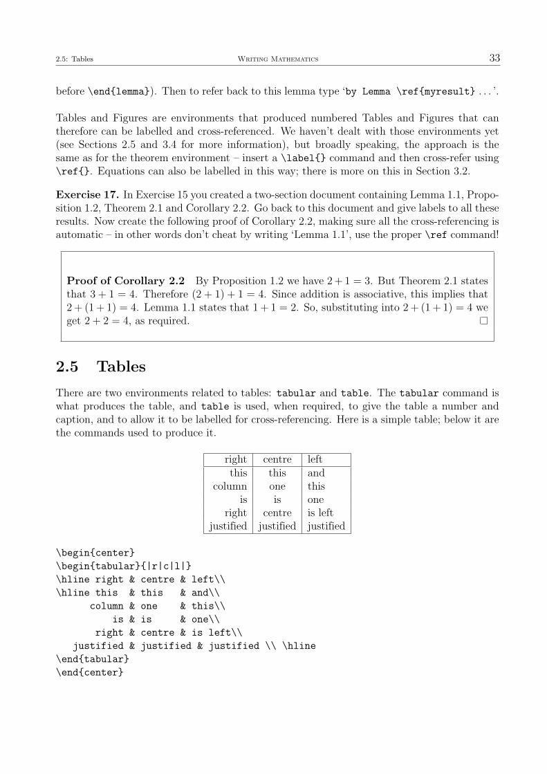
Exercise 17. In Exercise 15 you created a two-section document containing Lemma 1.1, Propo-sition 1.2, Theorem 2.1 and Corollary 2.2. Go back to this document and give labels to all theseresults. Now create the following proof of Corollary 2.2, making sure all the cross-referencing isautomatic – in other words don’t cheat by writing ‘Lemma 1.1’, use the proper \ref command!
Proof of Corollary 2.2 By Proposition 1.2 we have 2 + 1 = 3. But Theorem 2.1 statesthat 3 + 1 = 4. Therefore (2 + 1) + 1 = 4. Since addition is associative, this implies that2 + (1 + 1) = 4. Lemma 1.1 states that 1 + 1 = 2. So, substituting into 2 + (1 + 1) = 4 weget 2 + 2 = 4, as required.
2.5 Tables
There are two environments related to tables: tabular and table. The tabular command iswhat produces the table, and table is used, when required, to give the table a number andcaption, and to allow it to be labelled for cross-referencing. Here is a simple table; below it arethe commands used to produce it.
right centre leftthis this and
column one thisis is one
right centre is leftjustified justified justified
\begincenter
\begintabular|r|c|l|
\hline right & centre & left\\
\hline this & this & and\\
column & one & this\\
is & is & one\\
right & centre & is left\\
justified & justified & justified \\ \hline
\endtabular
\endcenter

34 Writing Mathematics Chapter 2: Progressing with LATEX
The first command needed is \begintabularcolumns. In the columns part you willdescribe the layout of each column. So, for example, rcl would mean that you want a right-justified column, followed by a centre-justified column, followed by a left-justified column,whereas ll would indicate two left-justified columns. Vertical lines can be drawn by inserting| at appropriate points. Thus in the table above we had |r|c|l|, which puts vertical lines beforeand after each column.
You do not need to specify how many rows the table will have. Within a row, each col-umn entry is separated by the ampersand &. The end of the row is denoted by a doublebackslash \\. To get horizontal lines we use the \hline command. Inserted at the startof a row it inserts a horizontal line above the current row. The final row is finished by the\endtabular command. But to get a line at the bottom of the table you finish the final rowwith \\ \hline \endtabular instead. Table 2.1 gives further examples of the commands.Additionally, though, we have put it into the table environment to show you how we cannumber, label and cross-reference tables.
1 a b ab1 1 a b aba a 1 ab bb b ab 1 aab ab b a 1
Table 2.1: Multiplication table for 1, a, b, ab
Table 2.1 was produced with the following commands.
\begintable[!hbt]
\begincenter
\begintabularc|cccc
& 1 & $a$ & $b$ & $ab$ \\
\hline 1 & 1 & $a$ & $b$ & $ab$ \\
$a$ & $a$ & 1 & $ab$ & $b$ \\
$b$ & $b$ & $ab$ & $1$ & $a$ \\
$ab$ & $ab$ & $b$ & $a$ & 1
\endtabular
\captionMultiplication table for $\1, a, b, ab\$
\labeltab1
\endcenter
\endtable
Note the optional argument [!hbt]. LATEX puts tables and figures where it thinks they will lookbest, not exactly where you have typed the commands for them. But you can (almost) insistwhere you want them to go. This particular command says ‘I really want you to put the table

2.5: Tables Writing Mathematics 35
right here, where I have written it. But failing that you can put it at the bottom of the page,and if it won’t fit there you can put it at the top.
It seems to matter to LATEX that you put the label after the caption, so I suggest you dothat! If you want the caption to be above the table, then put the \caption command after\begintable but before \begintabular.
On occasion you may wish to have entries that span more than one column of a table, ormore than one row, or lines that only cover part of the table. For this you will need the\multicolumncolspostext command and the \clinei-j command. The cols argu-ment is a number specifying how many columns should be spanned. The pos argument stateswhether this new merged column should be left, right or centre justified. The final argument,text, is the content of the merged column. The whole \multicolumn command is placed in thefirst column of the columns to be merged. For example in the instructions for Table 2.2 below,the second, third and fourth columns in the first row are merged.
DayTime Monday Tuesday Wednesday Thursday Friday
Morning Algebra Geometry Topology Rest AlgebraAfternoon Topology Analysis Rest Geometry TopologyEvening Rest Rest Algebra Analysis Rest
Table 2.2: Study Plan
The code that produced Table 2.2 is below. Note the need to put the vertical line | in themulticolumn argument, which makes sure that there is no gap in the right hand border of the‘Day’ cell.
\begintable[h!bt]
\begincenter
\begintabular|l||c|c|c|c|c|
\hline & \multicolumn5c|Day\\
\cline2-6
Time &Monday&Tuesday&Wednesday&Thursday&Friday\\
\hline \hline Morning&Algebra&Geometry&Topology&Rest&Algebra\\
\hline Afternoon&Topology&Analysis&Rest&Geometry&Topology\\
\hline Evening&Rest&Rest&Algebra&Analysis&Rest\\
\hline \endtabular
\captionStudy Plan \labeltab2
\endcenter
\endtable
Note that double lines (both vertical and horizontal) can be produced. In fact though, Table2.2 to my mind looks rather ugly and in general the minimalist style of Table 2.1 is often better.But it’s up to you.

36 Writing Mathematics Chapter 2: Progressing with LATEX
Exercise 18. Reproduce the following table (the mathematical symbols are \vee, \wedge and\Rightarrow).
Connectivesp q p ∨ q p ∧ q p⇒ qT T T T TT F T F FF T T F TF F F F T
2.6 Other useful commands
Footnotes
I’m not a great fan of footnotes in mathematical writing. If something is important it shouldbe stated in the main text. If it is not important then why are you saying it in the firstplace? However, if you do need to include one you should type \footnoteyour text. Yourfootnotes in any chapter will be numbered 1, 2, 3 and so on1. For some reason the footnotecommand doesn’t work within the title. To include one there you need to use the \thanks
command.
Exercise 19. In a new or existing document, create nine footnotes. Now add the command
\renewcommand*\thefootnote\fnsymbolfootnote
to the preamble and LATEX again. Note the result.
Forced Breaks
LATEX has been designed to produce professional looking layouts, and for the most part it doesa very good job. However sometimes its decisions about when to have a line break or a pagebreak may not be what you want for some reason. You can force line breaks and page breakswith the commands \linebreak, \newline, \pagebreak and \newpage. These commands haveslightly different effects. The \linebreak command stretches the line so that it is still left andright justified, whereas the \newline command simply ends the line where you have typedit. It is the same with \pagebreak and \newpage. Sometimes LATEX breaks a line betweenwords where you don’t want it to. For instance it looks silly to write ‘Theorem 2.1’ and see‘Theorem’ on the end of one line and 2.1 at the start of another. Equally, you wouldn’t want tosee ‘G. H. Hardy’ spread over two lines. To prevent this (or to correct it if it has occurred) youcan insert a tilde (˜): G.~H.~Hardy. This tells LATEX to keep these words or numbers together.
Exercise 20. Open a document containing at least two pages of text, for example the oneyou created for Exercise 13. Insert a \newpage command about halfway down the first page.Now try a \pagebreak command instead. Look at the difference in outcome. Do a similarexperiment with \linebreak and \newline.
1unless you specify otherwise in the preamble, see Exercise 19

Chapter 3
Mathematics
In this chapter we will look in more detail at more of the formatting you will need to produceproperly typeset mathematics. Section 3.1 discusses a few of the more common symbols andhow to work with them. Section 3.2 looks at numbered and un-numbered equations and thealign command which allows you to produced nicely aligned arrays of equations. Section 3.3deals with arrays and matrices. Then we have a look at figures and diagrams in Section 3.4.Some brief advice on writing style for mathematics follows in Section 3.5. Finally at the endof the chapter is a quick reference section for some of the more common mathematical symbolsand commands.
3.1 Symbols
We have already remarked that more or less any symbol you could ever need exists in LATEX.Section 3.6 consists of several tables containing the most common symbols that you might use,and the commands for them. Moreover in TEXStudio the left-hand navigation bars give mostof these symbols too. So generally it is easy to find the symbol you need. This section then ismore about guidance as to how to use symbols.
Dots
The position of dots matters. For example 9.3 means 9 310
but 9 · 3 means 9 × 3. The lowerdot is just the full stop on the keyboard. To get a centrally located dot you need \cdot. Thecentral dot is standard for scalar products (as in u · v), and common for group actions (as ing · x) and as a shorthand for multiplication (as in 9 · 8 · 7).
Another use for dots is to signify missing elements in lists or strings of various kinds. Theconvention here is that missing elements of a list be indicated by dots at the bottom of the line,whereas missing elements in a string of objects being combined in some way would be indicatedby central dots. We can also have diagonal or vertical dots, which are often used in matricesor other arrays (see Section 3.3). Over the page are some examples of these commands.

38 Writing Mathematics Chapter 3: Mathematics
1, 2, 3, . . . , n $\1, 2, 3, \ldots, n\$
1 + 2 + · · ·+ n $1 + 2 + \cdots + n$
1! = 1 $1! = 1$
2! = 2× 1 $2! = 2 \times 1$...
. . . $\vdots$ \hspace1.5cm $\ddots$
n! = n× · · · × 2× 1 $n! = n \times (n-1) \cdots \times 1$
Above and Below the Line
We have already seen in these notes several examples of superscripts and subscripts. A subscriptis obtained by use of an underscore _, and a superscript by use of a circumflex ^. Unlessotherwise instructed only the first character after the underscore or circumflex will be affectedby the command, so if you need more than one character in the subscript or superscript, youmust enclose all characters in curly brackets. The following examples show what I mean. Youmust be in mathematics mode to use these commands.
x2 $x^2$
x2/3 $x^2/3$
x2/3 $x^2/3$
a1 $a_1$
ai1 $a_i_1$
xai1i1
$x^a_i_1_i_1$
Subscripts and superscripts can be placed next to any symbol. Symbols like integrals, aswell as summation, product, union and intersection symbols, all often appear with subscriptsor superscripts. These symbols also have the property that they vary in size dependingon whether they are in a displayed equation or not. The context in which they appearalso determines how the subscripts and superscripts are shown. For example the command$\int_1^\infty x \mathrmdx$ results in
∫∞1
1xdx. But if we display it as an equation by
typing $$\int_1^\infty x \mathrmdx$$, we get instead:∫ ∞1
1
xdx.
Note that the ‘d’ in ‘dx’ is correctly given as a Roman ‘d’ not an italic ‘d’. Note also herethat fractions are automatically larger when in displayed equations. The default (larger) styleproduced for displayed equations is called displaystyle. The default smaller style producedfor in-line mathematics is called textstyle. You can demand that displaystyle be used ina line, or that textstyle be used in an equation by typing \displaystyle or \textstyle
immediately before your command. Hence
$\displaystyle\int_1^\infty \textstyle\frac1x \mathrmdx$

3.1: Symbols Writing Mathematics 39
produces
∫ ∞1
1xdx (note that we had to instruct LATEX to revert back to textstyle for the
fraction), and $$\int_1^\infty \textstyle\frac1x \mathrmdx$$ produces∫ ∞1
1xdx.
Here are some more examples of the textstyle and displaystyle forms of various symbols.
Expression textstyle displaystyle
\sum_r=1^n r^2∑n
r=1 r2
n∑r=1
r2
\prod_k \leq n x_k∏
k≤n xk∏k≤n
xk
\lim_x\rightarrow \infty e^-x limx→∞ e−x lim
x→∞e−x
\bigcap_A \in \mathcalA A⋂A∈AA
⋂A∈A
A
\bigcup_n \in \zz^+ [-n,n]⋃n∈Z+ [−n, n]
⋃n∈Z+
[−n, n]
Incidentally in this table, to fit the displayed mathematics in, I had to increase the amount ofspace allotted to the rows. To do this I used the command
\renewcommand\arraystretch1.6
immediately before the table, and then reset it immediately afterwards with
\renewcommand\arraystretch1.
Occasionally you may wish to place a symbol directly above or below another symbol, for exam-ple writing above an arrow. For this we use the overset and underset commands. For example,
the command $A \oversetf\longrightarrow B$ produces Af−→ B. The command
$A \undersetf\longrightarrow B$ produces A −→f
B. For each of these the main sym-
bol appears second and the annotation to it (the thing that will be overset or underset) is givenfirst.
Delimiters
Delimiters are symbols, usually appearing in pairs, that enclose expressions. We can haverounded ( ), curly , square [ ] and angled 〈 〉 brackets, each of which have particularmeanings and uses in mathematics. We will look at each of these in turn.

40 Writing Mathematics Chapter 3: Mathematics
Rounded Brackets These are used of course in normal text, but in the mathematical con-text tend to be reserved for co-ordinates, for row and column vectors and matrices, and forpermutations. Usually you will be able to produce them simply by using the left and rightbrackets on your keyboard. However sometimes this isn’t desirable, for example if enclosing alarge symbol such as
∑in brackets, you want the brackets to be large enough to enclose it.
Compare (n2 + 1
3n− 7) with
(n2 + 1
3n− 7
). To obtain the large brackets you type \left( and \right)
respectively. This works for all delimiters (I think!), even ones that don’t have an obvious rightand left, for example modulus signs. So \left|\frac27\right| gives
∣∣27
∣∣.Curly Brackets These are used for sets, and also to define functions in arrays – but we’lllook at arrays later in Section 3.3. A pitfall here is that as we know commands in LATEX oftenput arguments in curly brackets. Therefore LATEX treats them just as holders of information.Hence to really get curly brackets in your text you must type \ and \. Again if you wantcurly brackets that automatically adjust to be large enough for the text they contain, then youcan use \left\ and \right\.
Square Brackets These are used for closed intervals on the real line, for equivalence classesand sometimes in expressions where there are already lots of rounded brackets and a squarebracket looks less confusing. Again we can employ \left[ and \right] where necessary.
Angled Brackets These are usually used in the context of a set generating a group or vectorspace. You should used the dedicated symbols 〈 and 〉 rather than lazily writing ‘less than’ (<)or ‘greater than’ (>) symbols because the dedicated symbols look better and avoid confusion.
Here are some examples of these delimiters in use.
[0, 1] [0,1]
1
2,1
3 \\frac12, \frac13\ — doesn’t look very good
1
2,1
3
\left\\frac12, \frac13\right\ — that’s better
〈x : x5 = 1〉 \langle x: x^5 = 1\rangle
Other things to Note
Negation Symbols like = and ∈ have negations 6= (\neq) and /∈ (\notin). A few othernegations, providing you have the amssymb package in your preamble, are obtained by addingthe letter n before the command, as in (\ncong) and ≮ (\nless). If you try that and itdoesn’t work you can use the catch-all command \not. This command strikes a line throughwhatever immediately follows it. So $\not\equiv$ produces 6≡.

3.1: Symbols Writing Mathematics 41
Space Sometimes, marvellous as LATEX is, you may want to tweak the space allocated in amathematical expression. The following commands give a small amount of positive or negativespace. For complete control you can of course use the \hspace command, as in the last example.
\int \! \int∫ ∫
\int \int∫ ∫
\int \,\int∫ ∫
\int \;\int∫ ∫
\int \quad \int∫ ∫
\int \qquad \int∫ ∫
\int \hspace15mm \int∫ ∫
Trigonometric Functions Since letters typed in maths mode by default come out in italic,we need to take care when using functions like sin, cos and tan. Table 3.8 at the end ofthe chapter lists the functions to which this applies. The basic rule is that instead of typing$cos \theta$, for example, you should type $\cos \theta$. There may be occasions whenyou need to use a function for which there is not a predefined command. Suppose you want tolook at the least common multiple (lcm). You could type $\mathrmlcm$ whenever you useit in an equation, or you could define a new command in the preamble if you will be using it alot, for example the following.
\newcommand\lcm\mathrmlcm
Normal Text in Maths Mode Occasionally you will need to produce a few words of normaltext in Maths mode. This is best done using the \text command. If you try to do it with\mathrm or similar, you’ll find that words are run together and it looks awful. Compare thefollowing effects.
$\x \in X: x < a for all a \in A\$
$\x \in X: x < a \mathrmfor all a \in A\$
$\x \in X: x < a \textfor all a \in A\$
$\x \in X: x < a \text for all a \in A\$
x ∈ X : x < aforalla ∈ Ax ∈ X : x < aforalla ∈ Ax ∈ X : x < afor alla ∈ Ax ∈ X : x < a for all a ∈ A
Colons At the risk of accusations of perfectionism (!), I’ll make a small point about the useof colons. If you need to define a function, as in f : A → B, you need to use \colon ratherthan the keyboard character : to get the spacing right. Writing f:A\rightarrow B producesf : A→ B. This is spaced as if you are trying to express the ratio of ‘f ’ to ‘A→ B’, whereasthe \colon moves the resulting colon a little closer to the f .

42 Writing Mathematics Chapter 3: Mathematics
Exercise 21. Start a new document called ExCh3.tex. We will work on this document through-out the chapter.
• Use the \maketitle command to give your document a title (Exercises from Chapter 3)and an author (you!) but no date.
• Make sure that in the preamble you instruct LATEX to use the packages amsmath, amsfonts,amssymb and amsthm.
• Create a Section 1, called Symbols, containing the text below. (Don’t worry if you havedifferent text width and hence different linebreaks.)
Groups Let G be a group and X a set. We say that G acts on X if for all g ∈ Gthere is a map g : X → X such that the following hold.
1. For all x ∈ X we have 1G · x = x;
2. For all g1, g2 ∈ G and x ∈ X we have (g1g2) · x = g1 · (g2 · x).
Limits Using the algebra of limits we can deduce that
limn→∞
(2n2 + 3n+ 7
5n2 + 2n+ 3
)= lim
n→∞
(2 + 3 · ( 1
n) + 7 · ( 1
n2 )
5 + 2 · ( 1n) + 3 · ( 1
n2 )
)=
2
5.
Sets For each w in W there is a set of vectors N(w) with the property that for all
x, y ∈ W we have N(xy) = (N(y) \ [−y−1 ·N(x)])⋃y−1 (N(x) \N(y−1)) .
Exercise 22. Create a new command in your preamble. It should have the effect that whenyou type \tr in maths mode, the letters ‘tr’ (for trace) should appear in roman font. When youhave done that, use it to produce the following text in Section 1 of your document ExCh3.tex.
Let A be an n × n matrix. Then the trace of A, denoted tr(A), is the sum of theentries on the main diagonal of A. It can be shown that for all n× n matrices A andB we have tr(AB) = tr(BA).
Exercise 23. Create a new section(Section 2) in ExCh3.tex called An Interesting Function.Reproduce the following text in that section.

3.2: Equations Writing Mathematics 43
For a positive integer x we define g(x) to be 12x if x is even, and g(x) = 3x+ 1 if x is
odd. For example:
42 −→g
21 −→g
64 −→g
32 −→g· · · −→
g1.
We can define the following subset S of positive integers.
S = x ∈ Z+ : gn(x) = 1 for some n ∈ Z+
Conjecture We conjecture that S = Z+.
3.2 Equations
This section is about displayed mathematics. If you just want to display one equation centrallyon a line then you can use the double dollar signs I’ve mentioned. However I’ve read while pro-ducing these notes that using $$ is actually an old fashioned short cut, and that modern youngup-to-the-minute LATEXers always use \[ . . \] instead of double dollar signs. So maybe youshould too. This is all very well but for more complicated expressions, such as multi-line equa-tions and numbered equations, we need to look at a set of environments developed for thesepurposes. They are the equation, multline and align environments.
Before getting into details, note that in articles equations will be numbered (1), (2), (3) andso on. In books (or your dissertation), they will be numbered within chapters. In this currentbook we are in Chapter 3, so we have Equations (3.1) and (3.2) as the first two numberedequations in the chapter. Of course you can customise the numbering so that a different rule isfollowed in your document. If in an article you would like equations numbered by section, forexample, then you can include the following command in your preamble.
\numberwithinequationsection
The equation environment
The command \beginequation \labeleinstein E = mc^2 \endequation producesa numbered equation.
E = mc2 (3.1)
By giving it a label we can refer back to it in the text. There are two ways of doing this.You could write Equation \eqrefeinstein or Equation (\refeinstein). They bothproduce the same effect, namely ‘Equation (3.1)’. The standard \ref command only providesthe number, which is why with this option you must add the brackets yourself. If you want yourequation not to be numbered you can type \beginequation* E = mc^2 \endequation*.This is consistent with (for example) the distinction between numbered and unnumbered sec-

44 Writing Mathematics Chapter 3: Mathematics
tions (section and section*). Then we would just get the following output.
E = mc2
The multline environment
Equation (3.2) was produced using the \multline command, as shown below.
\beginmultline \labelmultex
\sum_r=1^12 r = 1 + 2 + 3 + 4 + 5
+ 6 + 7 + 8\\
+ 9 + 10 + 11 + 12 = 78
\endmultline
12∑r=1
r = 1 + 2 + 3 + 4 + 5 + 6 + 7 + 8
+ 9 + 10 + 11 + 12 = 78 (3.2)
Again we could have an unnumbered version using \beginmultline* and \endmultline*.This environment is useful for long expressions. It is much easier for the reader to absorb suchexpressions when they are not just included in lines of text.
Equation (3.2) is a slightly artificial example; usually when we want to break lines in anexpression it is because it is in the middle of a calculation over many lines. For such situationswe need the align environment.
The align environment
With a calculation spanning several lines, or indeed several equations displayed together, thecorrect method is to align them so that the equals signs are at the same position on the line.Naturally LATEX will do this for you automatically in the align environment. There is theflexibility to number every line, no lines or just some lines. Here are some examples.
\beginalign
\sin^2\theta + \cos^2\theta
& = 1 \labelcos\\
\sec^2\theta - \tan^2\theta
& = 1 \labeltan
\endalign
sin2 θ + cos2 θ = 1 (3.3)
sec2 θ − tan2 θ = 1 (3.4)
Notice that we have put a label on each line so that we can refer back to Equations (3.3) and(3.4) individually. The next example has no numbered lines.
\beginalign*
\pm\sqrtb^2 - 4ac
& = \pm\sqrt6^2 - 4\cdot (-2) \cdot 8\\
& = \pm\sqrt36 + 64\\
& = \pm\sqrt100 \\
& = \pm 10
\endalign*
±√b2 − 4ac = ±
√62 − 4 · (−2) · 8
= ±√
36 + 64
= ±√
100
= ±10

3.2: Equations Writing Mathematics 45
In the next example we have just numbered the last line.
\beginalign
\pm\sqrtb^2 - 4ac
& = \pm\sqrt6^2 -
4\cdot (-2) \cdot 8 \nonumber\\
& = \pm\sqrt36 + 64 \nonumber\\
& = \pm\sqrt100 \nonumber\\
& = \pm 10 \labelten
\endalign
±√b2 − 4ac = ±
√62 − 4 · (−2) · 8
= ±√
36 + 64
= ±√
100
= ±10 (3.5)
By adding further ‘&’ signs you can create arrays of equations. This can be useful if you havesimultaneous equations to solve. Here is an example.
a+ b = 2 b+ c = 5 c+ d = 7
d+ e = 9 e+ f = 11 f + a = 7
This was produced using the following commands.
\beginalign*
a + b & = 2 & b + c & = 5 & c + d & = 7 \\
d + e & = 9 & e + f & = 11 & f + a & = 7
\endalign*
There may be occasions when you wish to split a line inside a calculation. For that the simplestway is just to start a new line and leave a \quad space. If you are numbering every line you’llneed to insert a \nonumber command to avoid both halves of your split line being numbered.(There is a dedicated environment, the split environment, for this, but all it does is the no-number part, which you don’t need anyway most of the time as generally you’ll be using align*
rather than align.) Here’s an example of creating a split line manually.
\beginalign*
(x - y)(x^2 + xy + y^2)
& = x^3 + x^2y + xy^2 \\
& \quad - x^2y - xy^2 - y^3\\
& = x^3 - y^3
\endalign*
(x− y)(x2 + xy + y2) = x3 + x2y + xy2
− x2y − xy2 − y3= x3 − y3
Finally the align* environment can be useful when you wish to justify steps of your argument.
\beginalign* e^i\theta
&= \cos\theta + i\sin\theta
&& \text(by Theorem 7)\\
e^i\pi &= \cos\pi + i \sin \pi
&& (\textsetting \theta = \pi)\\
e^i\pi & = -1
\endalign*
eiθ = cos θ + i sin θ (by Theorem 7)
eiπ = cosπ + i sin π (setting θ = π)
eiπ = −1
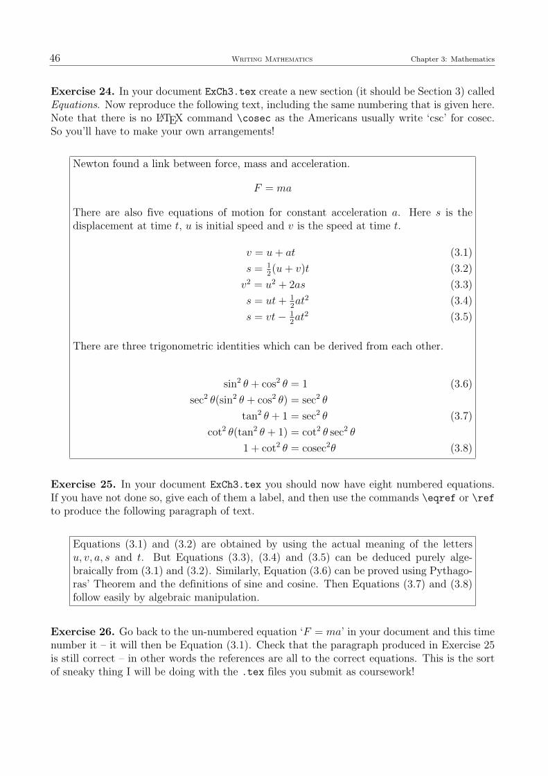
46 Writing Mathematics Chapter 3: Mathematics
Exercise 24. In your document ExCh3.tex create a new section (it should be Section 3) calledEquations. Now reproduce the following text, including the same numbering that is given here.Note that there is no LATEX command \cosec as the Americans usually write ‘csc’ for cosec.So you’ll have to make your own arrangements!
Newton found a link between force, mass and acceleration.
F = ma
There are also five equations of motion for constant acceleration a. Here s is thedisplacement at time t, u is initial speed and v is the speed at time t.
v = u+ at (3.1)
s = 12(u+ v)t (3.2)
v2 = u2 + 2as (3.3)
s = ut+ 12at2 (3.4)
s = vt− 12at2 (3.5)
There are three trigonometric identities which can be derived from each other.
sin2 θ + cos2 θ = 1 (3.6)
sec2 θ(sin2 θ + cos2 θ) = sec2 θ
tan2 θ + 1 = sec2 θ (3.7)
cot2 θ(tan2 θ + 1) = cot2 θ sec2 θ
1 + cot2 θ = cosec2θ (3.8)
Exercise 25. In your document ExCh3.tex you should now have eight numbered equations.If you have not done so, give each of them a label, and then use the commands \eqref or \ref
to produce the following paragraph of text.
Equations (3.1) and (3.2) are obtained by using the actual meaning of the lettersu, v, a, s and t. But Equations (3.3), (3.4) and (3.5) can be deduced purely alge-braically from (3.1) and (3.2). Similarly, Equation (3.6) can be proved using Pythago-ras’ Theorem and the definitions of sine and cosine. Then Equations (3.7) and (3.8)follow easily by algebraic manipulation.
Exercise 26. Go back to the un-numbered equation ‘F = ma’ in your document and this timenumber it – it will then be Equation (3.1). Check that the paragraph produced in Exercise 25is still correct – in other words the references are all to the correct equations. This is the sortof sneaky thing I will be doing with the .tex files you submit as coursework!

3.3: Arrays and Matrices Writing Mathematics 47
3.3 Arrays and Matrices
The array environment is essentially a tabular environment for mathematics. It can alignrows and columns of mathematics text, and is very versatile. The array environment is onlyallowed in maths mode, so in the example below it is included in an equation, but it could bejust between dollar signs, or in the align environment, or similar. Here is an example.
\beginequation*
f(x) =
\left\
\beginarrayll
\sqrtx & \textif x \geq 0\\
0 & \mboxotherwise
\endarray
\right.
\endequation*
f(x) =
√x if x ≥ 0
0 otherwise
You’ll see the array has two left-justified columns. Note also that only the left angled bracketis used. Because LATEX gets worried if left parentheses are not closed by right parentheses, weinsert a ‘dummy’ right parenthesis. The command \right. accomplishes this.
Arrays can also be used to produce matrices. But for simple matrices there are some dedicatedcommands which give you less control but are quicker. The commands are matrix, bmatrix,Bmatrix, pmatrix, vmatrix, Vmatrix and smallmatrix. For each of these you do not have tospecify how many columns or rows there are; you can just get typing. All columns are centrejustified and you don’t have the functionality of putting any vertical lines. Which is mostlyfine for simple examples. The different commands (except for smallmatrix) specify what kindof delimiter (bracket) goes around the matrix. The smallmatrix command produces a smallmatrix which can be used in a line. Here are some examples.
$\beginmatrix
1 & 2 \\ 3 & 4
\endmatrix$
1 2
3 4
$\beginbmatrix
1 & 2 \\ 3 & 4
\endbmatrix$
1 2
3 4
$\beginBmatrix
1 & 2 \\ 3 & 4
\endBmatrix$
1 2
3 4
$\beginpmatrix
1 & 2 \\ 3 & 4
\endpmatrix$
1 2
3 4

48 Writing Mathematics Chapter 3: Mathematics
$\beginvmatrix
1 & 2 \\ 3 & 4
\endvmatrix$
∣∣∣∣∣∣1 2
3 4
∣∣∣∣∣∣$\beginVmatrix
1 & 2 \\ 3 & 4
\endVmatrix$
∥∥∥∥∥∥1 2
3 4
∥∥∥∥∥∥$\beginsmallmatrix
1 & 2 \\ 3 & 4
\endsmallmatrix$
1 23 4
$\left(\beginsmallmatrix
1 & 2 \\ 3 & 4
\endsmallmatrix\right)$
( 1 23 4 )
Of these, the commands you are most likely to use are pmatrix and smallmatrix. However,there will be occasions when these quick commands do not produce the optimal outcome. Anexample of this is for matrices featuring negative numbers, or symbols, when left-justified orright-justified columns can be preferable. Below, for comparison, you can see a 3 × 3 matrixproduced using the pmatrix and array commands. The array version is clearly superior. Thefinal version illustrates the possibility, in the array environment, of including vertical and hor-izontal lines.
$\beginpmatrix
1 & 0 & \alpha\\
0 & -1 & \alpha^-1\\
0 & 0 & \alpha^2
\endpmatrix$
1 0 α
0 −1 α−1
0 0 α2
$\left(\beginarraycrl
1 & 0 & \alpha\\
0 & -1 & \alpha^-1\\
0 & 0 & \alpha^2
\endarray\right)$
1 0 α
0 −1 α−1
0 0 α2
$\left(\beginarraycr|l
1 & 0 & \alpha\\
0 & -1 & \alpha^-1\\
\hline 0 & 0 & \alpha^2
\endarray\right)$
1 0 α
0 −1 α−1
0 0 α2
One final special kind of array that has its own command is the binomial coefficient
(nr
); this
is produced with the command $\binomnm$.
Exercise 27. In Section 3 of ExCh3.tex create this text: g(x) =
12x if x is even;
3x+ 1 if x is odd.

3.4: Figures and Diagrams Writing Mathematics 49
Exercise 28. In your document ExCh3.tex use the appropriate matrix commands to produce
the following matrices:
a b
c d
,p q
r s
, ( 1 00 1 ), and
∣∣∣∣∣∣∣∣∣1 0 0
0 1 0
0 0 1
∣∣∣∣∣∣∣∣∣.
Exercise 29. In your document ExCh3.tex create the matrices
0 1 −1
1 2 3
and
1 0 ∗0 1 ∗
∗ ∗ 1
.
3.4 Figures and Diagrams
There are two aspects to the question of including graphics in documents. The first is gettingthem into the document; the second is actually creating them.
Importing Graphics
It is possible to include pictures and diagrams in your LATEX document if they are in one of thefollowing formats: pdf, eps, png, jpg, and gif. To do this, in the preamble to your document,you should insert the following line.
\usepackagegraphicx
If you need to use .eps files then you also need the epstopdf package. But I cannot think ofa case where you would be using a programme that can create .eps files but not .pdf files, soyou are not likely to need this.
At the point in the document where you want your picture to appear, you can simply type
\includegraphicsmypicture.pdf
(or mypicture.eps or mypicture.jpg or whatever file type your picture is). This will plonkyour picture straight into the text, which usually isn’t what you want! At the least you’llprobably want to display it:
\begincenter
\includegraphicsmypicture.pdf
\endcenter
You’ll often need to tweak pictures, for example scaling or rotating them. To do this you canuse the following example optional arguments in square brackets.
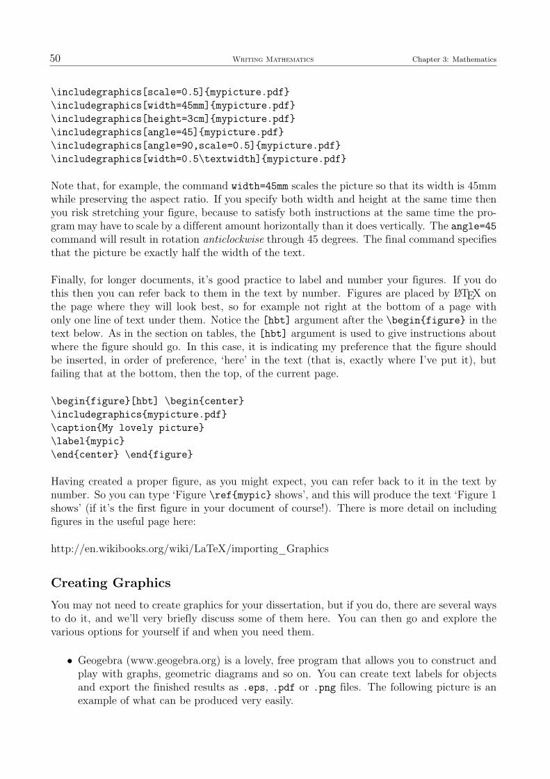
50 Writing Mathematics Chapter 3: Mathematics
\includegraphics[scale=0.5]mypicture.pdf
\includegraphics[width=45mm]mypicture.pdf
\includegraphics[height=3cm]mypicture.pdf
\includegraphics[angle=45]mypicture.pdf
\includegraphics[angle=90,scale=0.5]mypicture.pdf
\includegraphics[width=0.5\textwidth]mypicture.pdf
Note that, for example, the command width=45mm scales the picture so that its width is 45mmwhile preserving the aspect ratio. If you specify both width and height at the same time thenyou risk stretching your figure, because to satisfy both instructions at the same time the pro-gram may have to scale by a different amount horizontally than it does vertically. The angle=45
command will result in rotation anticlockwise through 45 degrees. The final command specifiesthat the picture be exactly half the width of the text.
Finally, for longer documents, it’s good practice to label and number your figures. If you dothis then you can refer back to them in the text by number. Figures are placed by LATEX onthe page where they will look best, so for example not right at the bottom of a page withonly one line of text under them. Notice the [hbt] argument after the \beginfigure in thetext below. As in the section on tables, the [hbt] argument is used to give instructions aboutwhere the figure should go. In this case, it is indicating my preference that the figure shouldbe inserted, in order of preference, ‘here’ in the text (that is, exactly where I’ve put it), butfailing that at the bottom, then the top, of the current page.
\beginfigure[hbt] \begincenter
\includegraphicsmypicture.pdf
\captionMy lovely picture
\labelmypic
\endcenter \endfigure
Having created a proper figure, as you might expect, you can refer back to it in the text bynumber. So you can type ‘Figure \refmypic shows’, and this will produce the text ‘Figure 1shows’ (if it’s the first figure in your document of course!). There is more detail on includingfigures in the useful page here:
http://en.wikibooks.org/wiki/LaTeX/importing_Graphics
Creating Graphics
You may not need to create graphics for your dissertation, but if you do, there are several waysto do it, and we’ll very briefly discuss some of them here. You can then go and explore thevarious options for yourself if and when you need them.
• Geogebra (www.geogebra.org) is a lovely, free program that allows you to construct andplay with graphs, geometric diagrams and so on. You can create text labels for objectsand export the finished results as .eps, .pdf or .png files. The following picture is anexample of what can be produced very easily.
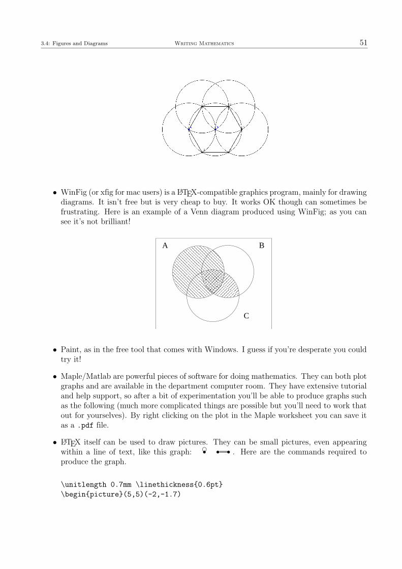
3.4: Figures and Diagrams Writing Mathematics 51
• WinFig (or xfig for mac users) is a LATEX-compatible graphics program, mainly for drawingdiagrams. It isn’t free but is very cheap to buy. It works OK though can sometimes befrustrating. Here is an example of a Venn diagram produced using WinFig; as you cansee it’s not brilliant!
A B
C
• Paint, as in the free tool that comes with Windows. I guess if you’re desperate you couldtry it!
• Maple/Matlab are powerful pieces of software for doing mathematics. They can both plotgraphs and are available in the department computer room. They have extensive tutorialand help support, so after a bit of experimentation you’ll be able to produce graphs suchas the following (much more complicated things are possible but you’ll need to work thatout for yourselves). By right clicking on the plot in the Maple worksheet you can save itas a .pdf file.
• LATEX itself can be used to draw pictures. They can be small pictures, even appearingwithin a line of text, like this graph: se s s . Here are the commands required toproduce the graph.
\unitlength 0.7mm \linethickness0.6pt
\beginpicture(5,5)(-2,-1.7)

52 Writing Mathematics Chapter 3: Mathematics
Figure 3.1: A Maple Picture
\put(0,0)\circle*2.00 \put(0,2)\circle3
\endpicture
%
\unitlength 0.7mm \linethickness0.6pt
\beginpicture(13,5)(-2,-1.7)
\put(0,0)\circle*2 \put(8,0)\circle*2
\put(1,0.7)\line(1,0)6 \put(1,-0.3)\line(1,0)6
\endpicture
Alternatively the pictures you draw can be full size diagrams incorporating text. I’vetaken the following diagram and commands from the ‘Not so short introduction to LATEX’,which was one of the documents in the recommended reading list and can be downloadedfrom the Moodle page for this module (or just by searching online – it’s freely available).Chapter 5 of that book is devoted entirely to producing graphics in LATEX, so I suggestyou read it!
\begincenter\setlength\unitlength0.8cm
\beginpicture(6,5)
\thicklines
\put(1,0.5)\line(2,1)3
\put(4,2)\line(-2,1)2
\put(2,3)\line(-2,-5)1
\put(0.7,0.3)$A$
\put(4.05,1.9)$B$
\put(1.7,2.95)$C$
\put(3.1,2.5)$a$
\put(1.3,1.7)$b$
\put(2.5,1.05)$c$

3.4: Figures and Diagrams Writing Mathematics 53
\put(0.3,4)$F= \sqrts(s-a)(s-b)(s-c)$
\put(3.5,0.4)$\displaystyle s:=\fraca+b+c2$
\endpicture
\endcenter
This set of instructions produces the picture below.
HH
HHH
A
B
Ca
bc
F =√s(s− a)(s− b)(s− c)
s :=a+ b+ c
2
• Finally, you can of course include photographs or other colour images, as these tendto be in .jpg format. You should be careful not to breach copyright if you are usingimages from books or the web, of course. The following is a (non-copyrighted) .jpg ofthe Mandelbrot set.
Exercise 30. Experiment with importing graphics, following the guidance below.
• Create a new section (Section 4) in your document ExCh3.tex, called Pictures. Includethe relevant package commands in the preamble for including graphics.
• Include a picture in Section 4. For example TrigGraph.pdf is Figure 3.1 from this section;it can be downloaded from the Moodle page for this module. Specify that the pictureshould be scaled to 20%.

54 Writing Mathematics Chapter 3: Mathematics
• Turn the picture you’ve imported into a figure, with a caption, and label it, for examplewith the command \labelgraph1 or something similar.
• Include the sentence ‘Figure 1 is the graph y = sin(x)(1+(ex)2)
.’
• Now import the picture four more times, creating captioned, labelled figures each time(so you end up with five figures in total). The first variation on Figure 1 should be 8cmwide. The second one should be 4cm high. The third should be both 8cm wide and 4cmhigh (look at the distortion that is created). The fourth should be half the size of Figure 1and rotated 90 degrees anticlockwise.
• Add some text which describes each figure, making sure to use the \ref command. Forexample, ‘Figure 2 is Figure 1 scaled to be 10cm wide’.
• Finally, change the order of your figures with a bit of cutting and pasting, and make surethat the text still refers to the correct figures.
3.5 Good Mathematical Writing
So far we have concentrated mostly on simply processing your mathematics and text withLATEX. There are whole books on good writing and I do not intend to write another one. Inthis section I will content myself with ten tips for making your mathematics easier to read andunderstand.
1. Think about structure. In a long report or dissertation, you should have chapters, sectionsand probably subsections. A good structure might be to have an introductory chaptersetting up notation, terminology, basic concepts and results, then a chapter for eachspecific topic. Sections can split up the topic of a chapter further. Each new thoughtrequires a new paragraph. The structure should be natural and not feel forced or arbitrary.
2. The page layout should not be too dense. This means that you should avoid havingvery narrow margins, and acres of uninterrupted text. Display equations rather thanshoehorning lots of mathematics into lines. Start new paragraphs when necessary.
3. Define any notation you use if there is the slightest room for doubt about what it couldmean, or if a fairly competent undergraduate might not recognise it. So you don’t needto define Z and R, for example, but if using N you should state for the record whetheryou are using it to mean the set of positive integers or the set of non-negative integers.
4. In the mathematics itself, pay attention to detail. Avoid death by subscript. If yournotation requires something horrid like xijk , then it is not good notation! Avoid usingsymbols that look too similar to each other. For example the Greek letters upsilon andnu both look rather like each other and like the letter v in maths mode: υ, ν, v. So itwould be foolhardy to use them together.

3.5: Good Mathematical Writing Writing Mathematics 55
5. Follow convention. Variables are usually x, y, z. Constants are usually a, b, c. Scalars areoften λ and µ. Vectors are usually u,v,w. Complex numbers are usually z or w. Thereare subject specific conventions too. Groups are usually G, H. Normal subgroups areoften N and K. Try to avoid using notation that normally means something else. So ifyou have a group G and want to consider an arbitrary subgroup, don’t call that subgroupG′ because this is fairly standard notation for the commutator subgroup of G. Similarlyyou should probably avoid calling anything but the identity matrix I and, if there arecomplex numbers floating about, using i as anything other than the square root of minusone is bound to lead to trouble.
6. Use the proper tools. If you want angled brackets, for example, then use them. Don’tuse the less than and greater than symbols. This is not mere pedantry. Using the wrongsymbols can cause confusion. For example the expression < xi|i < n > is hard to decipher,whereas 〈xi|i < n〉 is much easier.
7. Use the numbering, labelling and cross-referencing functionality provided by LATEX. Avoidsaying things like ‘by the lemma above’. There may be several previous lemmas to whichyou could be referring. This also goes for lazily writing Lemma 1 (for example) ratherthan Lemma \reflemma1. You are a hostage to fortune when you go back and add,delete or move something in the editing process. But only number the equations to whichyou will refer back. In particular there is usually no need to number every single line ofa long calculation. Mostly you should use the align* environment here.
8. Abbreviations should be avoided. This includes things like e.g., i.e., etc., wlog, wrt, iff,⇒, ⇔, ∴ and ∵, though at a push QED is probably acceptable. While these are oftenused informally (and by lecturers on the whiteboard) they are not correct in a formaldocument.
9. Do not break off in the middle of a proof to state and prove a supplementary result. Beforeembarking on a proof you should have proved all the required lemmas and propositionsthat are needed to establish your main theorem and can then reference them in theproof. If a proof is very long, consider proving some parts of it separately (beforehand)as lemmas.
10. Treat mathematical symbols as part of the text, and do not overuse them. It is mucheasier for the reader to see ‘Let x and y be positive integers’ than ‘Let x ∈ Z+, y ∈ Z+’.You should also make sure that you are producing grammatical sentences, even wheremathematical symbols are used. You can test this by reading it to yourself. Here is a badsentence: ‘Let x ∈ S, x > 7.’ This reads, ‘let x in S, x is greater than 7’. What you reallywant to say is: ‘let x be an element of S such that x is greater than 7’. This could beslightly shortened to ‘let x be an element of S such that x > 7. A similar example is ‘LetA ⊆ B be a subset’, which reads ‘Let A be a subset of B be a subset’ ! Better to write‘let A be a subset of B’. Do your best to avoid starting a sentence with a mathematicalsymbol. This is considered bad form!

56 Writing Mathematics Chapter 3: Mathematics
3.6 Quick Reference
The tables in this handy ‘cut out and keep’ guide were originally prepared by David Carlisleat Manchester University, and he kindly shared them online. One or two of the more unusualsymbols require the package amssymb.
α \alpha θ \theta o o τ \tau
β \beta ϑ \vartheta π \pi υ \upsilon
γ \gamma γ \gamma $ \varpi φ \phi
δ \delta κ \kappa ρ \rho ϕ \varphi
ε \epsilon λ \lambda % \varrho χ \chi
ε \varepsilon µ \mu σ \sigma ψ \psi
ζ \zeta ν \nu ς \varsigma ω \omega
η \eta ξ \xi
Γ \Gamma Λ \Lambda Σ \Sigma Ψ \Psi
∆ \Delta Ξ \Xi Υ \Upsilon Ω \Omega
Θ \Theta Π \Pi Φ \Phi
Table 3.1: Greek Letters
± \pm ∩ \cap \diamond ⊕ \oplus
∓ \mp ∪ \cup 4 \bigtriangleup \ominus
× \times ] \uplus 5 \bigtriangledown ⊗ \otimes
÷ \div u \sqcap / \triangleleft \oslash
∗ \ast t \sqcup . \triangleright \odot
? \star ∨ \vee C \lhd © \bigcirc
\circ ∧ \wedge B \rhd † \dagger
• \bullet \ \setminus E \unlhd ‡ \ddagger
· \cdot o \wr D \unrhd q \amalg
+ + − -
Table 3.2: Binary Operation Symbols
a \hata a \acutea a \bara a \dota a \brevea
a \checka a \gravea ~a \veca a \ddota a \tildea
Table 3.3: Math mode accents

3.6: Quick Reference Writing Mathematics 57
≤ \leq ≥ \geq ≡ \equiv |= \models
≺ \prec \succ ∼ \sim ⊥ \perp
\preceq \succeq ' \simeq | \mid
\ll \gg \asymp ‖ \parallel
⊂ \subset ⊃ \supset ≈ \approx ./ \bowtie
⊆ \subseteq ⊇ \supseteq ∼= \cong on \Join
@ \sqsubset A \sqsupset 6= \neq ^ \smile
v \sqsubseteq w \sqsupseteq.= \doteq _ \frown
∈ \in 3 \ni ∝ \propto = =
` \vdash a \dashv < < > >
: :
Table 3.4: Relation Symbols
← \leftarrow ←− \longleftarrow ↑ \uparrow
⇐ \Leftarrow ⇐= \Longleftarrow ⇑ \Uparrow
→ \rightarrow −→ \longrightarrow ↓ \downarrow
⇒ \Rightarrow =⇒ \Longrightarrow ⇓ \Downarrow
↔ \leftrightarrow ←→ \longleftrightarrow l \updownarrow
⇔ \Leftrightarrow ⇐⇒ \Longleftrightarrow m \Updownarrow
7→ \mapsto 7−→ \longmapsto \nearrow
← \hookleftarrow → \hookrightarrow \searrow
\leftharpoonup \rightharpoonup \swarrow
\leftharpoondown \rightharpoondown \nwarrow
\rightleftharpoons \leadsto
Table 3.5: Arrow Symbols
. . . \ldots · · · \cdots... \vdots
. . . \ddots
ℵ \aleph ′ \prime ∀ \forall ∞ \infty
~ \hbar ∅ \emptyset ∃ \exists \Box
ı \imath ∇ \nabla ¬ \neg ♦ \Diamond
\jmath√
\surd [ \flat 4 \triangle
` \ell > \top \ \natural ♣ \clubsuit
℘ \wp ⊥ \bot ] \sharp ♦ \diamondsuit
< \Re ‖ \| \ \backslash ♥ \heartsuit
= \Im ∠ \angle ∂ \partial ♠ \spadesuit
f \mho . . | |
Table 3.6: Miscellaneous Symbols

58 Writing Mathematics Chapter 3: Mathematics
∑\sum
⋂\bigcap
⊙\bigodot∏
\prod⋃
\bigcup⊗
\bigotimes∐\coprod
⊔\bigsqcup
⊕\bigoplus∫
\int∨
\bigvee⊎
\biguplus∮\oint
∧\bigwedge
Table 3.7: Variable-sized Symbols
\arccos \cos \csc \exp \ker \limsup \min \sinh
\arcsin \cosh \deg \gcd \lg \ln \Pr \sup
\arctan \cot \det \hom \lim \log \sec \tan
\arg \coth \dim \inf \liminf \max \sin \tanh
Table 3.8: Log-like Symbols
( ( ) ) ↑ \uparrow ⇑ \Uparrow
[ [ ] ] ↓ \downarrow ⇓ \Downarrow
\ \ l \updownarrow m \Updownarrow
b \lfloor c \rfloor d \lceil e \rceil
〈 \langle 〉 \rangle / / \ \backslash
| | ‖ \|
Table 3.9: Delimiters
\rmoustache \lmoustache
\rgroup \lgroup \arrowvert
ww \Arrowvert \bracevert
Table 3.10: Large Delimiters
abc \widetildeabc abc \widehatabc←−abc \overleftarrowabc
−→abc \overrightarrowabc
abc \overlineabc abc \underlineabc︷︸︸︷abc \overbraceabc abc︸︷︷︸ \underbraceabc√abc \sqrtabc
n√abc \sqrt[n]abc
f ′ f’ abcxyz
\fracabcxyz
Table 3.11: Some other constructions

Chapter 4
Presentations
This chapter is about preparing presentations using LATEX. As part of your dissertation module,you will be giving two presentations. The first is a short, informal one (the Preliminary presen-tation) at the end of the Autumn Term in your second year. For this you may well choose (orindeed have chosen!) to simply write on the whiteboard, though some people do prefer havingeverything written in advance on slides, even for a short presentation. The main presentation isa different matter. This is a 20 minute final presentation of your project, to be given shortly af-ter you submit your finished dissertation. Lecturers and fellow students will be present, and youwill wish to give a polished performance. This chapter is written with that presentation in mind.
The main tool used for preparing LATEX presentations is the beamer package. In the first sectionof this chapter we will start by creating a very simple presentation. In subsequent sections wewill look at creating a title page, choosing ‘themes’ (which determine colour schemes and soon), using the ‘Birkbeck’ theme, slide layout, effects such as gradual reveal, and guidelines forgood presentation design. The aim here is to give you a brief overview, enough so that youcan prepare a competent presentation. As ever, LATEX is almost infinitely customisable. Veryfull documentation about the beamer class is given in the Beamer User Guide. At 245 pagesit really does tell you everything you could want to know. It is freely available online and alsoon the Moodle page for this module.
4.1 A simple presentation
The following commands produce a presentation consisting of a single slide.
Preamble \documentclassbeamer
\usepackageamsfonts,amsmath,amssymb
Begin Document \begindocument
A slide \beginframe
This is my first slide.
\endframe
End Document \enddocument

60 Writing Mathematics Chapter 4: Presentations
As you can see, slides are produced as ‘frames’ and are created in the frame environment. Theresulting document is shown over the page.
This is my first slide.
Notice that the font is a sans serif font (called computer modern). Fonts such as this are easierto read in presentations and their clean lines make for a better looking slide. It is possible toalter the size and typeface but not without effort. We will look briefly at this in Section 4.3. Atthe bottom of the slide there are various symbols. These are navigation tools that are presentin the default beamer style. We’ll discuss them when we have a slightly longer document tonavigate through.
To create more slides you simply add more frames. Adding the following text to the simplepresentation above will create a second slide containing the text ‘This is my next slide.’
\beginframe
This is my next slide.
\endframe
Exercise 31. Create a presentation called myslides.tex, consisting of four slides each con-taining one line of text.
Frames may be given titles (and even subtitles) as shown in Example 4.1. You will also seethat standard LATEX commands work here, but the results are slightly different. Theorems, forexample, are not numbered (or, to be more precise, the numbers are not shown).
Example 4.1. The following commands will produce a frame of output.
\beginframe
\frametitleFractions don’t exist
\begintheorem
The smallest positive number is 1.

4.1: A simple presentation Writing Mathematics 61
\endtheorem
\beginproof
Let $x$ be the smallest positive number. Clearly $x \leq 1$. Now $x^2$ is also
positive, so by minimality of $x$, $x \leq x^2$. Divide both sides by (the
positive number) $x$ to get $1 \leq x$. Thus $1 \leq x \leq 1$. Hence $x=1$.
\endproof
\begincorollary
All numbers are integers.
\endcorollary
\endframe
The above input creates the following frame.
Fractions don’t exist
TheoremThe smallest positive number is 1.
Proof.Let x be the smallest positive number. Clearly x ≤ 1. Now x2 isalso positive, so by minimality of x , x ≤ x2. Divide both sides by(the positive number) x to get 1 ≤ x . Thus 1 ≤ x ≤ 1. Hencex = 1.
Corollary
All numbers are integers.
You may be looking at a black and white printout, in which case note that the title and thewords theorem, proof and corollary are blue here. That is the default beamer style.
We could have added a subtitle using the command \framesubtitleThis is a lie, orsimilar.
Exercise 32. In your presentation myslides.tex or elsewhere, add titles to your pages, andsubtitles to two of the pages. Add a new first page which is the page created in Example 4.1.

62 Writing Mathematics Chapter 4: Presentations
Here is a closer view of the navigation symbols on the slides.
This is my first slide.
Working left to right, the symbols represent slides, frames, subsections and sections. Clickingto the left or right of each symbol causes you to jump backward or forward one slide, frame,subsection or section respectively. (The difference between a slide and a frame is that in theoryit is possible to have a frame over-run into more than one slide. This is best avoided as manyof the commands, such as gradual reveal and titling, won’t work. So for our purposes slidesand frames are the same.) The final symbols are undo, search and redo.
You can nagivate your way around the final pdf document by pressing the up and down arrowkeys on your keyboard. For a short presentation you will have so few slides that this will sufficeand you may not wish to go to the trouble of dividing your document into sections. The usualreason for making these subdivisions in a standard article is that we are numbering things andcross-referring. We also have different sizes of headings and so on. But in a presentation it isbest to avoid numbering completely. No-one will remember what ‘Theorem 2.1’ was. For thisreason the commands \section and \subsection do not have the same effect in the beamerclass. They do not create headings, for example. In a document without sections most of thesenavigation tools then become redundant, and so they have been omitted from the Birkbeckpackage introduced in Section 4.4.
4.2 Creating a Title Page
Your presentation needs a title page. As with titles in articles and other LATEX documents, thisis achieved by stating the title, author, date and so on, and then issuing a command to producethe title. Here it is \titlepage rather than \maketitle.
After \begindocument the following commands will produce the title page shown on theright.
\titleA Presentation on False Proofs
\authorG.~Otcha
\instituteBirkbeck College
\dateSeptember 20th
\beginframe
\titlepage
\endframe
A Presentation on False Proofs
G. Otcha
Birkbeck College
September 20th

4.3: Themes Writing Mathematics 63
Note that if you have a very long title, author or date, you can have an optional argument insquare brackets with a short version. For example
\date[20th September]Just after six o’clock on the twentieth day of September
You would do this if your presentation theme (see the next section) shows the title, date orauthor at the top or bottom of each frame.
Exercise 33. Add a title page to your document myslides.tex.
4.3 Themes
The style of a presentation is called a theme. If nothing is specified in the preamble, thenthe default theme is used. It has a white background, blue headings, no left or right sidebars,and small navigation buttons at the bottom of the page. There are many ways in which youcan change the style of your presentation. The most major change is the presentation theme,but you can also vary colour schemes and choice of font within that. It is possible to changeindividually almost any detail of the slide and presentation structure, but there is no real needto do this unless you wish to. More or less you will simply choose a presentation theme andcolour scheme from the available options.
Presentation Themes
These are wholesale specifications for every aspect of a presentation: colour scheme, the sym-bols used for lists, the font, what sidebars are shown, and so on. Presentation Themes arenamed after cities. An example is madrid. To specify a theme include the line (for example)\usethemeMadrid in the preamble. If you do not specify a theme then the default themewill be used. For a list of available presentation themes see the Beamer User Guide, which isavailable online, including on the Moodle page for this module. Maura Paterson has designeda Birkbeck Presentation Theme which is the subject of the next section.
On the next page you see the slide from Example 4.1. The only change is the addition ofa \usetheme command to the preamble. The page on the left results from the command\usethemeMadrid. The page on the right results from the command \usethemeWarsaw.
Note that Warsaw shows section and subsection titles at the top of the page. Also note if youare looking at a black and white printout that the colour scheme for these is blue.

64 Writing Mathematics Chapter 4: Presentations
Fractions don’t exist
Theorem
The smallest positive number is 1.
Proof.
Let x be the smallest positive number. Clearly x ≤ 1. Now x2 is alsopositive, so by minimality of x , x ≤ x2. Divide both sides by (the positivenumber) x to get 1 ≤ x . Thus 1 ≤ x ≤ 1. Hence x = 1.
Corollary
All numbers are integers.
G. Otcha (Birkbeck College) A Presentation on False Proofs September 20th 2 / 6
Errors in Proofs Algebra
Fractions don’t exist
Theorem
The smallest positive number is 1.
Proof.
Let x be the smallest positive number. Clearly x ≤ 1. Now x2 isalso positive, so by minimality of x , x ≤ x2. Divide both sides by(the positive number) x to get 1 ≤ x . Thus 1 ≤ x ≤ 1. Hencex = 1.
Corollary
All numbers are integers.
G. Otcha A Presentation on False Proofs
Colour Themes
A colour theme only controls the colour palette of the presentation. If no command is given, thedefault colour theme for your chosen presentation theme will be used. To specify a colour themeinclude after choosing your main theme, the line (for example) \usecolorthemeseagull.Note: color has the American spelling! The seagull theme, for example, creates variousgreys for the backgrounds. Below you will see the sample page from Example 4.1. The page onthe left results from the command \usethemeBerkeley in the preamble. The page on theright results from inserting into the preamble the command \usethemeBerkeley followed bythe command \usecolorthemealbatross.
APresentationon FalseProofs
G. Otcha
Errors inProofs
Algebra
Fractions don’t exist
Theorem
The smallest positive number is 1.
Proof.
Let x be the smallest positive number. Clearly x ≤ 1. Now x2
is also positive, so by minimality of x , x ≤ x2. Divide bothsides by (the positive number) x to get 1 ≤ x . Thus1 ≤ x ≤ 1. Hence x = 1.
Corollary
All numbers are integers.
Beamer colour themes are mostly named after flying animals, such as beetle, dove, fly. It isalso possible to dictate precise colour changes, such as the colour of one sidebar. However youthen risk picking colours that look awful together! Again, for a list of standard colour themessee the Beamer User Guide.
Exercise 34. Modify your presentation myslides.tex as follows. Firstly create at least onesection and at least one subsection. This is done with the usual section and subsection

4.3: Themes Writing Mathematics 65
commands, which should be placed between frames. Then experiment with the presentationthemes Madrid, Frankfurt, Copenhagen and Antibes, and the colour themes albatross, dove,spruce and beetle.
Font Themes
Obviously these themes specify fonts. It is unlikely that you will need to alter standard settingsvery much, but there are one or two commands here that may be of use. We have remarked thatthe text in presentations is by default sans serif. This is mostly fine except that in mathematicswe are so used to seeing serif fonts that it is often easier on the eye to typeset mathematicsin this way. To achieve serif mathematics while retaining the rest of the document in sansserif font, add the line \usefonttheme[onlymath]serif to the preamble after specifyingyour theme. Over the page you will see, for comparison, two slides; the one on the rightmakes use of the \usefonttheme[onlymath]serif command. The page on the left doesnot. While consistency of typeface is usually desirable, you may feel that, depending on thecontent of your presentation, the introduction of serifs for mathematics may well be worthwhile.
Here is a slide comparing the way mathematics looks in sans serifand serif fonts.
1. For n ∈ Z, we have n ≤ n2.
2. If x ∈ R and 0 < |x | < 1 then x2 < x .
3. The area of a circle of radius r is πr2.
4. If sin θ = l , then |11 sin θ| ≤ |11l |.5. The identity matrix is usually denoted I .
Here is a slide comparing the way mathematics looks in sans serifand serif fonts.
1. For n ∈ Z, we have n ≤ n2.2. If x ∈ R and 0 < |x| < 1 then x2 < x.
3. The area of a circle of radius r is πr2.
4. If sin θ = l, then |11 sin θ| ≤ |11l|.5. The identity matrix is usually denoted I.
Inner and Outer Themes
Inner themes alter things that happen inside a frame. That is, in the body of the slide ratherthan any sidebars, borders, headers and footers. You can change symbols used for lists, the wayin which theorems are shown (in a box or not, for example) and other things. Outer themesgovern page layout – the style and contents of any headers, footers and sidebars. For the mostpart you are likely to be happy with the set-up of whatever presentation theme you use. Seethe Beamer User Guide for more information.
Remember that the rationale for choosing given themes, or elements of themes, is ease ofcomprehension. Any changes you make should be justifiable in terms of making the talk easierto follow.

66 Writing Mathematics Chapter 4: Presentations
4.4 A Birkbeck Presentation
Maura Paterson has designed a special Birkbeck package for presentations which is availablefor Birkbeck students and staff to use. To do so, you will need to download the following filesfrom Moodle.
bbklogo.jpg
beamerthemebbk2.sty
You should be sure to save these files in the same directory as the presentation for which youwill be using them.
Maura has also give permission for you to access the .tex file of a presentation she preparedon her research, using the Birkbeck theme. The file is called khoptalk.tex and again you candownload it from Moodle or the computer lab.
To use the Birkbeck theme, you will need to insert the following lines into your preamble.
\usethemebbk2
\usefontthemestructurebold
\usepackagegraphicx
You can include the Birkbeck logo in your title page too. The following is a basic documentthat uses the Birkbeck theme, and which you can modify as you wish.
Preamble \documentclassbeamer
\mode<presentation>
\usethemebbk2
\usefonttheme[onlymath]serif
\usepackagegraphicx
Begin Document \begindocument
Title Page \title[False Proofs]A Presentation on False Proofs
\authorG.~Otcha
\institute[Birkbeck College]
Department of Economics, Mathematics and Statistics\\
Birkbeck, University of London\\ \vspace0.7cm
\includegraphics[width=2cm]bbklogo
\dateSeptember 20th
\beginframe\titlepage\endframe

4.4: A Birkbeck Presentation Writing Mathematics 67
A slide \beginframe
\frametitleSummary of Results
My research is fascinating.
\endframe
End Document \enddocument
Exercise 35. Create a presentation using the Birkbeck theme, by modifying your myslides.tex
presentation accordingly (or starting from scratch).
You will have noticed that the Birkbeck logo is in fact inserted manually into the title page, sothat even using the Birkbeck presentation theme, you are not compelled to use the logo, norindeed to mention the word ‘Birkbeck’ anywhere. The job of the theme is to set up the look ofthe slides. The colour scheme uses Birkbeck college colours (dark red, essentially) and sets upthe structure of slides. You will see below the title page and a sample slide from a presentationusing the Birkbeck theme. The nagivation symbols are omitted on the grounds that they arenot useful during a short talk, and section headings are not shown. What is shown is theauthor’s name and the current slide number. This gives both you and the audience a feel forhow far through the talk you are. If you have three minutes to go and are on slide 3 of 15, youmay see some worried faces!
A Presentation on False Proofs
G. Otcha
Department of Economics, Mathematics and StatisticsBirkbeck, University of London
September 20th
G. Otcha False Proofs 1/2
Fractions don’t exist
Theorem
The smallest positive number is 1.
Proof.
Let x be the smallest positive number. Clearly x ≤ 1. Now x2 isalso positive, so by minimality of x, x ≤ x2. Divide both sides by(the positive number) x to get 1 ≤ x. Thus 1 ≤ x ≤ 1. Hencex = 1.
Corollary
All numbers are integers.
G. Otcha False Proofs 2/2
The title page commands would work in other presentation themes too of course. As a finalpossibility, if you are feeling brave you may modify the style file beamerthemebbk2.sty tocreate different results.
Note: For reasons that I do not understand, occasionally when a new frame is added LATEXtakes more than one attempt to realise that the total number of slides has gone up. So youmay add a slide, LATEX your work and see that it is labelled slide 6/5 or something similarlyridiculous. This will fix itself on the next running of LATEX but always check the page numberingwhen you have finished preparing the presentation.

68 Writing Mathematics Chapter 4: Presentations
4.5 Creating Slides
Having established the overall look of your presentation with presentation and colour themes,it is now time to think about the content of, and layout within, the slides themselves. Broadlyspeaking, standard LATEX commands work more or less as expected. There are a few exceptions.You can create as many slides (frames) as you like. If you write too much text in any one frame,it will overspill to another slide, and you’ll need to add another frame when you spot this. Thecommand \frametitleTitle will give your slide a title; if you don’t want that slide to havea title, just omit this command.
Numbering
We have already remarked that theorems, examples and other environments that are numberedby LATEX will not appear to be numbered in a presentation. People won’t remember thingsby number. If you want to refer back to a result you have stated, it is sensible to either giveit a name (for example Lagrange’s Theorem, or ‘The Main Theorem’) or to restate it whenrequired. Hopefully in a short presentation you will only have a handful of results and will beable to distinguish easily between them.
Lists
For the most part it is not necessary to have numbered lists. But the enumerate environmentwill produce them for you, should you so desire. For bulleted lists, which is what you are likelyto need, you can use the itemize environment as usual. On a slide, lists are often a useful andclear way of getting information across. Below is a sample slide from a presentation preparedin the Birkbeck theme. The itemize environment has been used on the left; the enumerate
environment on the right.
Living Things
I vertebratesI birdsI mammals
I sheepI cows
I invertebratesI arachnidsI insects
I plants
1. vertebrates
1.1 birds1.2 mammals
1.2.1 sheep1.2.2 cows
2. invertebrates
2.1 arachnids2.2 insects
3. plants
G.Otcha False Proofs 6/5

4.5: Creating Slides Writing Mathematics 69
Items in sublists of each type are shown in a smaller font size. The symbol indicating items inan itemized list is always the same, a triangle, but the placement on the frame, and the sizeof the text, clearly indicates list level. In the enumerated list on the right, you will see thatthe numbering is 1, 1.1, 1.1.1 and so on. In other presentations the symbols differ. You canexperiment, and of course as ever all these things can be changed if you try hard enough. Asan example of a different theme’s treatment of lists, the following is the same sample frame,but using the presentation theme Madrid.
Living Things
vertebrates
birdsmammals
sheepcows
invertebrates
arachnidsinsects
plants
1 vertebrates1 birds2 mammals
1 sheep2 cows
2 invertebrates1 arachnids2 insects
3 plants
A.Student (Birkbeck College) Sample Slide September 20th 6 / 6
Emphasis
The \em command does work, but since we have colour available to us, you may prefer to usethe \alert command. The default setting is that it turns the selected text red. So to highlightthe phrase ‘at least one’ in the following sentence, you would use the following raw tex.
Every cubic equation has \alertat least one real solution.
Figures and Tables
The \includegraphics command works in Beamer as with standard documents. You will needto think about the way in which you show pictures. Think carefully about whether you needto label figures and give them titles. After all you will be there explaining what the diagramsare at the time. Similar advice goes for tables. Note that any placement options for figuresand tables will be ignored by Beamer. It simply places figures and tables as they are put in thetext. This is because slides contain so little material that specifying ‘top’, ‘here’ or ‘bottom’ isnot so vital. The outcome is that you have more control. You can place text next to figures ortables using the columns environment, which we are about to discuss. It is possible to includesounds, film clips and animations too, but I do not expect many of you to need this option,which requires the multimedia package. See the Beamer User Guide for more information.

70 Writing Mathematics Chapter 4: Presentations
Columns
It can be useful to divide the page, or parts of the page, up into columns, probably at mosttwo. This is done using the following commands.
\begincolumns
\begincolumn0.45\textwidth
whatever you want in your first column
\endcolumn
\begincolumn0.45\textwidth
whatever you want in your second column
\endcolumn
\endcolumns
The width of the column is defined in this example to be slightly less than half the width ofthe text, though you can specify an exact width if you wish, in millimetres (mm), centimetres(cm), inches (in) or points (pt). As long as the total width of your combined columns does notexceed the total textwidth, anything goes.
The columns environment is flexible in that a frame can contain parts with different numbersof columns.
Example 4.2. The following text outputs a frame with a theorem (across the whole page)followed by two columns of text.
\beginframe\frametitleA Sample Slide
\begintheorem[Sylow’s Theorems]
Let $G$ be a group of order $p^nm$, where $p$ is prime, $n \in \mathbbZ^+$
and $m$ is a positive integer coprime to $p$. Then $n_p$, the number of
subgroups of $G$ having order $p^n$, divides $|G|$ and moreover
\[n_p \equiv 1 \modp.\]
\endtheorem
We can divide the page into columns.
\begincolumns
\begincolumn0.45\textwidth
\beginitemize
\item Very important information.
\item $e^i\pi = -1$
\item $E=mc^2$
\enditemize
\endcolumn

4.5: Creating Slides Writing Mathematics 71
\begincolumn0.45\textwidth
\beginenumerate
\item Numbered lists can be useful.
\item But only if you need to refer back to items in the list.
\endenumerate
\endcolumn
\endcolumns
\endframe
Here is the resulting output.
A Sample Slide
Theorem (Sylow’s Theorems)
Let G be a group of order pnm, where p is prime, n ∈ Z+ and mis a positive integer coprime to p. Then np, the number ofsubgroups of G having order pn, divides |G| and moreover
np ≡ 1 mod p.
We can divide the page into columns.
I Very importantinformation.
I eiπ = −1I E = mc2
1. Numbered lists can beuseful.
2. But only if you need torefer back to items in thelist.
G.Otcha False Proofs 4/4
Each column is essentially a (small) page in its own right. This has the consequence thatcommands like \textwidth, when used in a column, reference the width of the text in thecolumn, not the whole page. This affects things like the specification of widths for includedgraphics. Consider the following commands for a column.
\begincolumn0.5\textwidth
\includegraphics[width=.5\textwidth]picture.pdf
\endcolumn
This would produce a column half the width of the frame. The picture inside that columnwould be half the width of the column, which means it would be a quarter of the width of thepage.
A final observation about this sample slide: notice that the theorem is given a name (Sylow’sTheorems). The name is formatted as part of the title of the theorem. To achieve this therelevant command was \begintheorem[Sylow’s Theorems].

72 Writing Mathematics Chapter 4: Presentations
Exercise 36. In your presentation myslides.tex use the columns environment to add a framecontaining six figures (any pictures you like). One figure on the top, two figures below andthree below that. It might look something like the slide below.
G.Otcha False Proofs 5/5
4.6 Effects
In this section we will look at two main effects: overlays, where you reveal different parts ofyour slide at different times, and transition effects, which govern the way one frame changes tothe next. Remember that any effect should enhance what you are saying, not distract from it.
Overlays and Gradual Reveal
Just as in a powerpoint presentation, you can reveal the information on your slides gradually.The sequence of gradually changing slides is called the set of overlays. A single frame mayconsist of several overlay slides. As with all effects, you shouldn’t do it just because you can,but sometimes it can be useful to only show part of an argument, to keep the audience focusedon what is being discussed at that moment.
There are two main ways to produce overlays. The simplest is the \pause command. You simplyinsert this command wherever you want a pause in the text. Then during the presentation youjust hit the page down, or enter, key, to proceed to the next point.
Example 4.3. The following sample frame uses the pause command. It will consist of fouroverlay slides.
\beginframe
\frametitleAn English Nursery Rhyme
\beginblockTwinkle Twinkle Little Star\pause
Twinkle twinkle little star,\\
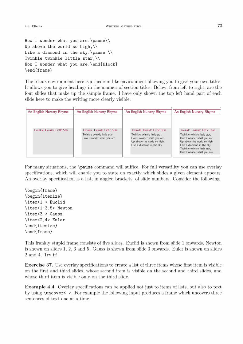
4.6: Effects Writing Mathematics 73
How I wonder what you are.\pause\\
Up above the world so high,\\
Like a diamond in the sky.\pause \\
Twinkle twinkle little star,\\
How I wonder what you are.\endblock
\endframe
The block environment here is a theorem-like environment allowing you to give your own titles.It allows you to give headings in the manner of section titles. Below, from left to right, are thefour slides that make up the sample frame. I have only shown the top left hand part of eachslide here to make the writing more clearly visible.
An English Nursery Rhyme
Twinkle Twinkle Little Star
Twinkle twinkle little star,How I wonder what you are.Up above the world so high,Like a diamond in the sky.Twinkle twinkle little star,How I wonder what you are.
A.Student Sample Slide 7/7
An English Nursery Rhyme
Twinkle Twinkle Little Star
Twinkle twinkle little star,How I wonder what you are.
Up above the world so high,Like a diamond in the sky.Twinkle twinkle little star,How I wonder what you are.
A.Student Sample Slide 7/7
An English Nursery Rhyme
Twinkle Twinkle Little Star
Twinkle twinkle little star,How I wonder what you are.Up above the world so high,Like a diamond in the sky.
Twinkle twinkle little star,How I wonder what you are.
A.Student Sample Slide 7/7
An English Nursery Rhyme
Twinkle Twinkle Little Star
Twinkle twinkle little star,How I wonder what you are.Up above the world so high,Like a diamond in the sky.Twinkle twinkle little star,How I wonder what you are.
A.Student Sample Slide 7/7
For many situations, the \pause command will suffice. For full versatility you can use overlayspecifications, which will enable you to state on exactly which slides a given element appears.An overlay specification is a list, in angled brackets, of slide numbers. Consider the following.
\beginframe
\beginitemize
\item<1-> Euclid
\item<1-3,5> Newton
\item<3-> Gauss
\item<2,4> Euler
\enditemize
\endframe
This frankly stupid frame consists of five slides. Euclid is shown from slide 1 onwards, Newtonis shown on slides 1, 2, 3 and 5. Gauss is shown from slide 3 onwards. Euler is shown on slides2 and 4. Try it!
Exercise 37. Use overlay specifications to create a list of three items whose first item is visibleon the first and third slides, whose second item is visible on the second and third slides, andwhose third item is visible only on the third slide.
Example 4.4. Overlay specifications can be applied not just to items of lists, but also to textby using \uncover< >. For example the following input produces a frame which uncovers threesentences of text one at a time.
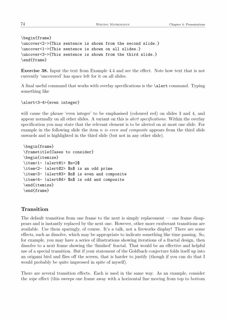
74 Writing Mathematics Chapter 4: Presentations
\beginframe
\uncover<2->This sentence is shown from the second slide.
\uncover<1->This sentence is shown on all slides.
\uncover<3->This sentence is shown from the third slide.
\endframe
Exercise 38. Input the text from Example 4.4 and see the effect. Note how text that is notcurrently ‘uncovered’ has space left for it on all slides.
A final useful command that works with overlay specifications is the \alert command. Typingsomething like
\alert<3-4>even integer
will cause the phrase ‘even integer’ to be emphasised (coloured red) on slides 3 and 4, andappear normally on all other slides. A variant on this is alert specifications. Within the overlayspecification you may state that the relevant element is to be alerted on at most one slide. Forexample in the following slide the item n is even and composite appears from the third slideonwards and is highlighted in the third slide (but not in any other slide).
\beginframe
\frametitleCases to consider
\beginitemize
\item<1- |alert@1> $n=2$
\item<2- |alert@2> $n$ is an odd prime
\item<3- |alert@3> $n$ is even and composite
\item<4- |alert@4> $n$ is odd and composite
\enditemize
\endframe
Transition
The default transition from one frame to the next is simply replacement — one frame disap-pears and is instantly replaced by the next one. However, other more exuberant transitions areavailable. Use them sparingly, of course. It’s a talk, not a fireworks display! There are someeffects, such as dissolve, which may be appropriate to indicate something like time passing. So,for example, you may have a series of illustrations showing iterations of a fractal design, thendissolve to a next frame showing the ‘finished’ fractal. That would be an effective and helpfuluse of a special transition. But if your statement of the Goldbach conjecture folds itself up intoan origami bird and flies off the screen, that is harder to justify (though if you can do that Iwould probably be quite impressed in spite of myself).
There are several transition effects. Each is used in the same way. As an example, considerthe wipe effect (this sweeps one frame away with a horizontal line moving from top to bottom

4.6: Effects Writing Mathematics 75
gradually replacing it with the next). If you wish the transition from frame k to frame k+ 1 touse the wipe effect, then after the line \beginframe that starts frame k + 1, insert the line
\transwipe
Note: I have found that these effects are only visible in the external (adobe acrobat) pdfviewer, and moreover it has to be in full screen mode.
You can change the duration of these effects — the default is 1 second. To cause the wipe effectto last 0.3 seconds, you would use the command
\transwipe[duration=0.3]
For some of the effects you can specify the direction in which the effect proceeds. So for thewipe effect the default is that the screen is wiped with a horizontal line moving downwardsfrom top to bottom. You may change the direction using the option [direction=], with thenumber 0, 90, 180 or 270. For example
\transwipe[direction=180]
causes the frame to be wiped by a vertical line moving from right to left. The full list of effectsis as follows.
Command Effect
\transblindshorizontal like horizontal blinds being closed
\transblindsvertical like vertical blinds being closed
\transboxin old frame collapses to a point in the centre
\transboxout new frame emerges as a growing box from the centre
\transdissolve old frame dissolves into new
\transglitter dissolve combined with wipe left to right
\transsplithorizontalin new slide replaces old from top and bottom
\transsplithorizontalout new slide spreads from central horizontal line
\transsplitverticalin new slide replaces old from left and right
\transsplitverticalout new slide spreads from central vertical line
\transwipe new slide sweeps away old from top to bottom
Exercise 39. Add transition effects to a presentation. Experiment with duration and directionof different effects.
76 Writing Mathematics Chapter 4: Presentations
4.7 Printing your presentation
You are likely to want to print out your presentation so that you can read it over, make noteson it and have a hard copy in case of some technical disaster. But if you simply print the pdf ofyour presentation as it stands, there is likely to be a problem. Any frame that has been gradu-ally revealed using the \uncover or \pause commands, or overlay specifications, is created byproducing a new pdf page for each overlay. So, for example, a list whose six items have beenrevealed one by one will result in six pages of output. What we need is a way to suppress theseoverlay commands. That way is by adding the option ‘handout’ to the document class.
\documentclass[handout]beamer
and changing the ‘mode’ (if this command is in your document) from \mode<presentation> to\mode<handout>. If your background colour on frames is white, then it can help to distinguishslides by tweaking it slightly for the handouts, even if you change nothing else. To accomplishthis, you can add an option specification to the handout mode.
\mode<handout>\setbeamercolorbackground canvasbg=black!5
The effect of this is that the background colour changes from white to a very pale grey.
When printing a handout you will typically wish to print at least two and probably four frameson each page. The easiest way of doing so is probably to use the package pgfpages in yourpreamble as follows:
\usepackagepgfpages
\pgfpagesuselayout4 on 1[a4paper,border shrink=5mm,landscape]
Instead of 4 on 1 you can just print 2 pages on 1, and then you should remove the ‘landscape’option. A sample page of a printout with four frames on each page, is shown on the final pageof this chapter.
Exercise 40. Create a version of your myslides presentation that uses the handout overlayspecifications. You might wish to choose a different colour and/or presentation theme for thehandout. Now print (or at least get a print preview of) your presentation.
4.8 Ten Guidelines for a Good Presentation
1. Get the length right. One slide per minute is already pushing it. Better to plan somethingaround ten to fifteen slides at most for a 20 minute presentation. Of course you willpractice it and you should ruthlessly cull anything that doesn’t fit. If you are runningshort of time, omit slides rather than simply speaking faster!
2. The amount of material on any one slide should not be large. If your text doesn’t fit onthe slide, take this as a sign that you need to redesign or reword the slide. Do not take

4.8: Ten Guidelines for a Good Presentation Writing Mathematics 77
it as a sign that you should remove all spacing and have five columns just to wedge it in.
3. Avoid numbering things unless there is a good reason. In this list the points are numberedto emphasise the fact that there are ten of them. That may well not be a sensible reason!
4. Choose a sensible presentation theme. All information on all slides should be useful insome way.
5. Try to avoid including long calculations, detailed tables or other text that requires closeand careful reading. In a presentation you are usually trying to give the big picture, ratherthan elucidate all the detail. Your dissertation may well contain complex formulae, andlarge tables of data, but a table with, say, 7 rows and 8 columns contains over 50 entries;no-one can take that information in, unless your talk consists entirely of that one slide.
6. Don’t introduce too much new notation. People cannot remember it. If your first slidesays ‘let G be a group, p a prime, q a power of p, r a positive integer, H a subgroup of G,N a normal subgroup of G, set K = H ∩ N , k = |K|, a ∈ G, b ∈ H, c ∈ N and d ∈ K’then you, and the audience, are doomed. Either people will just stop listening, or youwill be plagued with interruptions as people ask ‘what was K again?’
7. It is useful to have a final page that says something like, ‘The End’ or ‘Thank you’ oryour email address, or similar. It signals the end of the talk without that embarrassingtailing off that can occur, where it gradually becomes clear to the audience, and you, thatyou have said everything you are going to say.
8. Practice your talk, out loud. That swanky Greek letter you used — can you rememberwhether it’s a zeta or an eta? One of the great things about LATEX is that you have toknow the name of Greek letters in order to type them. But what about ./ or ∼. Are yougoing to refer to them in your talk as ‘bowtie’ and ‘sim’? You also need to know how topronounce, at least roughly, the names of any famous mathematicians you mention. Ifin doubt, ask your supervisor. If they don’t know, then you are probably safe to get itwrong! Otherwise, get it right.
9. Prepare for disaster. If you lose your USB stick, would you be able to cope? Make sureyou have a printed copy of the talk so that in an emergency you could give an abbreviatedversion of the talk on a whiteboard. Better, make sure you have backed up your talk ontoeither a second USB stick, or email it to yourself so you can access it online. And of courseturn up in good time so that you can make sure your talk is set up on the computer, andyou are not out of breath or flustered.
10. Prepare for questions. Try and think of the sort of questions you may get asked, andprepare answers. If you are asked something you don’t know, it isn’t a disaster. Try andgive some sort of a response, which could range from ‘I don’t know the answer in generalbut if n = 3 the answer is this.’ to ‘I know that was mentioned in Jones’s book, I can’trecall the exact result but research has been done in that area’, or similar. Sometimesyou may just have to say you don’t know, but there is often something that you can say,however small.

78 Writing Mathematics Chapter 4: Presentations
Sam
plePresentation
A.Student
Dep
artmen
tofEco
nomics,
Mathem
atics
andStatistics
Birk
beck
,University
ofLondon
Septem
ber
20th
A.Studen
tSample
Presen
tatio
n1/4
Fractions
don’texist
Theorem
Thesm
allestpositive
number
is1.
Proof.
Let
xbethesm
allestpositive
number.
Clearly
x≤
1.Now
x2is
alsopositive,
soby
minim
alityof
x,x≤
x2.
Divid
eboth
sides
by(th
epositive
number)
xto
get1≤
x.Thus1≤
x≤
1.Hence
x=
1.
Corollary
Allnumbers
areintegers.
A.Studen
tSample
Presen
tatio
n2/4
ASam
pleSlide
Theorem
(Sylow
’sTheorem
s)
Let
Gbeagrou
pof
order
pnm,where
pisprim
e,n∈Z+andm
isapositive
integer
coprimeto
p.Then
np ,
thenumber
ofsubgrou
psof
Ghavin
gord
erpn,divid
es|G|andmoreover
np ≡
1modp.
Wecan
divid
ethepage
into
columns.
IVery
importan
tinform
ation.
Ieiπ
=−1
IE
=mc2
1.Numbered
listscan
be
usefu
l.
2.Buton
lyifyou
need
torefer
back
toitem
sin
the
list.
A.Studen
tSample
Presen
tatio
n3/4
Living
Things
Ivertebrates
Ibird
sI
mam
mals
Isheep
Icow
s
IinvertebratesI
arachnids
Iinsects
Iplan
ts
1.vertebrates
1.1bird
s1.2
mam
mals
1.2.1
sheep
1.2.2
cows
2.invertebrates
2.1arach
nids
2.2insects
3.plan
ts
A.Studen
tSample
Presen
tatio
n4/4

Chapter 5
Dissertations
A dissertation is a rather longer document than we have worked with so far, but after yourpractice with writing articles, producing the actual content will not require many new skills.The main new things to get to grips with will be the document classes, such as book, thatallow for chapters, and the creation of a title page, abstract, declaration, table of contents andbibliography. As with presentations, we have a Birkbeck project package for dissertations thatyou have the option of using. It sets up many of the format requirements for you.
5.1 Layout of a Dissertation
There are several things that need to be included in your dissertation, however you choose toprepare it. When you start your dissertation module you will receive a formal list of require-ments, but as a guide the following rules will need to be observed.
• Your dissertation must be typed.
• It must be on white A4 paper, single sided.
• It must be at least 10 point and at most 12 point font.
• Lines must be at least 1.5 spaced and at most double spaced.
• Margins must be at least 30mm.
• Pages must be numbered.
• There must be a title page including the title of the dissertation and your name.
• There must be an abstract.
• There must be a declaration stating that the work is your own.
• There must be a bibliography.

80 Writing Mathematics Chapter 5: Dissertations
Other things, such as a table of contents, are optional but highly desirable. Although nota formal requirement, you will of course wish to divide your dissertation into well-organisedchapters, containing sections and maybe subsections. You will label these chapters and sections,as well as theorems, figures, tables, relevant equations and so on, so that you can refer back tothem. This is done in the same way as discussed in earlier chapters.
Word Count
As you may recall, your dissertation should be between 6,000 and 10,000 words. This is a widerange, to reflect the fact that a project heavy in calculation would have relatively few wordscompared to a more discursive dissertation. Please don’t count your words by hand! TEXstudiohas a tool that counts words – and it doesn’t count the words used in commands, so it is justwhat is required. Go to Tools, click on Analyse Text, and then on Count. It will give, as wellas a word count, a frequency analysis of words used. But what you care about is word count.I have just checked and in the first four chapters of these notes there are 24,841 words. Whichmeans 1,000 words would cover about 3 single-spaced pages on average. Of course your projectis going to be double spaced, which will make it look much more impressive!
5.2 Choice of Document Class
There are several choices of document class, but the two I will talk about are report (inconjunction with the Birkbeck style file) and book.
The ‘Report’ Class
This is the simplest document class that produces chapters. There are no headers, and thefooter is a central page number. The assumption is that the report is being printed on singlesided paper and so there is no difference in format between odd and even numbered pages. The\maketitle command produces a separate title page with the title, author and date as usual.To use the report class, the first line of your preamble should be \documentclassreport.Or in fact, more likely you would type \documentclass[a4paper,12pt]report. But we cando better than this.
The Birkbeck Project Style
We have prepared a style file bbkproject.sty that you can use in conjunction with the report
class. The style file can be downloaded from the Moodle page for this module. It sets up thestructure of the document so that you can create a title page, abstract, declaration and tableof contents, the line spacing is correct, the margins are the right size and so on. The pagedesign reflects the fact that we would like the dissertation to be submitted single sided. Thatmeans all page numbers are on the top right. You do not need to look at the contents of thebbkproject.sty file unless you wish to. To use the Birkbeck project package bbkproject, thefirst two lines of your preamble should be:
5.2: Choice of Document Class Writing Mathematics 81
\documentclass[a4paper,12pt]report
\usepackagebbkproject
Of course you must have the file bbkproject.sty in the same folder as your dissertation.
With this package the headers and footers are set up as follows.
• No header or footer on the title page.
• On the first page of each chapter, and for the abstract, declaration and table of contents,there are no headers and the footer is just the page number.
• No difference between odd and even numbered pages, because the dissertation is supposedto be single sided.
• Header of standard page: on the left the current chapter number and title; on the right,the page number.
• Footer of standard page: on the right the current section number and title.
There are other advantages to using this package: it is easy to produce the abstract and dec-laration that are required. Moreover the margins and line spacing are set up as per guidelines.Finally a table of contents is automatically produced. However it is certainly not compulsoryto use this package.
The ‘Book’ Class
The book class is another class that produces chapters. These notes have been produced usingthe book class. It expects that the outcome will be viewed in book form — pages printed onboth sides, so that odd and even numbered pages are formatted separately. A chapter alwaysbegins on an odd numbered page (the right hand page of a book). That means if your Chapter1 ends on page 9 say, then page 10 will be left blank so that Chapter 2 can begin on page11. For your dissertation the book class is not optimal, because you are asked to produce asingle-sided document, but you may wish to use it in future. Headers and footers are set up asfollows.
• No header or footer on the title page
• Title, contents and chapters begin on odd numbered pages.
• On the first page of each chapter, and for the abstract, declaration and table of contents,there are no headers and the footer is just the page number.
• Header of standard even numbered (left hand) page: page number on left, Chapter numberand name in upper case text on the right. No footer.
• Header of standard odd numbered (right hand) page: page number on right, sectionnumber and name in upper case text on the left. No footer.

82 Writing Mathematics Chapter 5: Dissertations
• Left margin of even numbered page is wider than right margin. Right margin of oddnumbered page is wider than left margin.
Headers and footers can be altered using the fancyhdr package. Since we are supplying aBirkbeck package already, I will not go into detail about doing this. But to give you an idea ofthe sort of thing that can be done, look at the headers and footers of these notes. The relevantcommands from the preamble are as follows.
\documentclass[12pt,a4paper]book
\usepackagefancyhdr
\pagestylefancyplain
\addtolength\headwidth\marginparsep
\addtolength\headwidth\marginparwidth
\addtolength\headheight2.5pt
\renewcommand\chaptermark[1]\markboth
\scriptsize Chapter \thechapter : #1
\renewcommand\sectionmark[1]\markright\scriptsize \thesection : #1
\lhead[\fancyplain\thepage]\fancyplain\rightmark
\rhead[\fancyplain\leftmark]\fancyplain\thepage \cfoot
\chead[\fancyplain\textsc\scriptsize Writing Mathematics]
\fancyplain\textsc\scriptsize Writing Mathematics
\textwidth 170mm \oddsidemargin -4mm \evensidemargin -6mm
\textheight 227mm \topmargin -5mm
You will see commands like \lhead, which deals with the left hand side of the header, givinginstructions for odd numbered and even numbered pages. The default in this package is thatthe header is underlined, unlike using the book class on its own. I do not expect you to beconversant with all of this. But you are welcome to explore the fancyhdr package if you wish.
5.3 Title Page, Abstract, Declaration
In this section we will look at how to produce a title page, abstract and declaration, focusingmainly on how this is done in files using the bbkproject package.
The Title Page
Example 5.1. If using bbkproject, insert the following lines into your preamble.
\subjectMathematics
\degreeM.Sc.
\thesisdissertation
\titleA Short Proof of Fermat’s Last Theorem
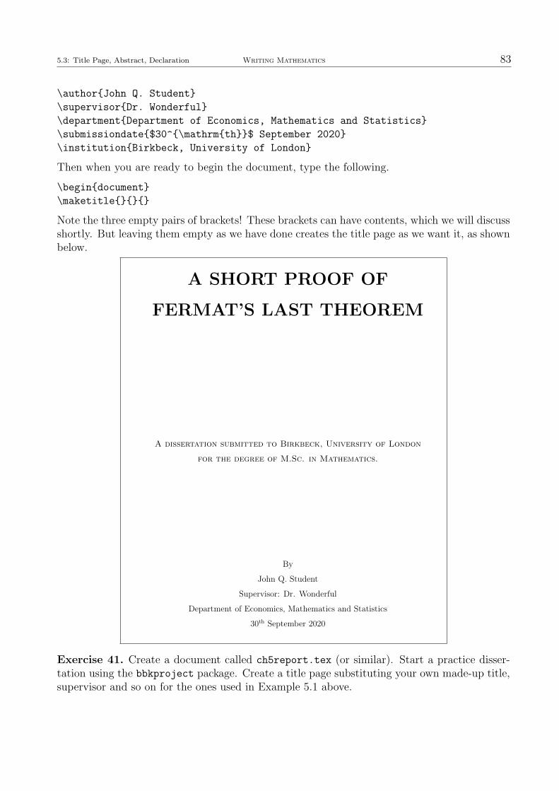
5.3: Title Page, Abstract, Declaration Writing Mathematics 83
\authorJohn Q. Student
\supervisorDr. Wonderful
\departmentDepartment of Economics, Mathematics and Statistics
\submissiondate$30^\mathrmth$ September 2020
\institutionBirkbeck, University of London
Then when you are ready to begin the document, type the following.
\begindocument
\maketitle
Note the three empty pairs of brackets! These brackets can have contents, which we will discussshortly. But leaving them empty as we have done creates the title page as we want it, as shownbelow.
A SHORT PROOF OF
FERMAT’S LAST THEOREM
A dissertation submitted to Birkbeck, University of London
for the degree of M.Sc. in Mathematics.
By
John Q. Student
Supervisor: Dr. Wonderful
Department of Economics, Mathematics and Statistics
30th September 2020
Exercise 41. Create a document called ch5report.tex (or similar). Start a practice disser-tation using the bbkproject package. Create a title page substituting your own made-up title,supervisor and so on for the ones used in Example 5.1 above.

84 Writing Mathematics Chapter 5: Dissertations
Exercise 42. Create a document called ch5book.tex (or similar). This time start a practicedissertation using the document class book. Create a title page.
If you are not using the bbkproject package, then you can create a title page with Title,Author and Date with the standard \maketitle command.
The Abstract
Your dissertation must have an abstract. This is a short (around one page) summary of whatyou have done. It is important because it allows the Programme Director to assign the mostappropriate second examiner, and it allows the two internal examiners and the external exam-iner to assess your ability to give a clear summary of the scope and results of your project.
In the bbkproject package, insert your abstract in the third argument of the \maketitle
command. As an example, the command
\maketitleI have found a beautiful proof,
but this abstract is too short to contain it.
produces, in conjunction with the preamble commands from Example 5.1, the following abstractpage.
Abstract
BIRKBECK, UNIVERSITY OF LONDON
ABSTRACT OF DISSERTATION submitted by John Q. Student and enti-
tled A Short Proof of Fermat’s Last Theorem.
Date of Submission: 30th September 2020
I have found a beautiful proof, but this abstract is too short to contain it.
4

5.3: Title Page, Abstract, Declaration Writing Mathematics 85
If you are not using the bbkproject package, then you can create an abstract using the com-mand
\chapter*Abstract
and then typing your abstract. But it won’t have all the nice layout above.
Exercise 43. Add an abstract to your document ch5report.tex, which you created in Exercise41 using the bbkproject package. Next, add an abstract to your document ch5book.tex, whichyou created in Exercise 42 using the book document class.
The Declaration
Another necessary component of your dissertation is the declaration that you are aware ofplagiarism rules, have read them, and that you have not plagiarised. You need to include thetext of the declaration when you submit your dissertation. If you are using the bbkproject
package, then the declaration is automatically included, as shown.
Declaration
This dissertation is submitted under the regulations of
Birkbeck, University of London as part of the examina-
tion requirements for the M.Sc. degree in Mathematics.
Any quotation or excerpt from the published or unpub-
lished work of other persons is explicitly indicated and in
each such instance a full reference of the source of such
work is given. I have read and understood the Birkbeck
College guidelines on plagiarism and in accordance with
those requirements submit this work as my own.
5

86 Writing Mathematics Chapter 5: Dissertations
If you are not using the bbkproject package, you can create a page with the declaration on byusing the command
\chapter*Declaration
and then typing the words of the declaration. They will not be nicely centred on the pagethough. This can be achieved using the \minipage command, which we will describe in moredetail in Section 5.5.
5.4 Table of Contents
LATEX has the ability to generate a table of contents automatically from the chapter, sectionand subsection structure. If you are using the bbkproject package, a table of contents will beautomatically generated after your title page. It is a good thing to have and you need to thinkcarefully about your reasons for not wanting one, should you decide to omit it.
There is one decision you need to make, and that is about the depth of your table of contents.It will show chapters, and sections within chapters, and subsections too unless you specify oth-erwise. My view is that while showing chapters and sections is helpful, it is not necessary to godown to the level of subsections and subsubsections. I therefore suggest inserting the command
\setcountertocdepth1
into your preamble. Depth 0 is the highest level – for the case of a book or report, that ischapters. Depth 1 is the next level, here sections. Depth 2 is subsections and so on. Byspecifying depth 1, we say that the table of contents should list chapters and sections but nosmaller subdivisions. This will work with or without the bbkproject package. If you are notusing the bbkproject package, a table of contents will not automatically appear. If you wantone, you need to type the command
\tableofcontents
after the \maketitle command.
If your dissertation has lots of tables or lots of figures, or both, you might want to have a list oftables and/or a list of figures. Some books do this. One case where this might be useful for thereader is if you have tables summarising all the data about some different cases. So maybe youhave some investigation to do with prime numbers, and a table at the end of Chapter 2 withinformation about the case p = 2, one at the end of Chapter 3 with information about the casep ≡ 1 mod 4 and then a final one about the case p ≡ 3 mod 4. Then the reader could findthese tables quickly by looking for the page references in the list of tables. You will need tomake a judgement as to whether it helps the reader to have these lists. To insert them if usingthe bbkproject package, you use the first two arguments of the redefined \maketitle

5.5: Chapters Writing Mathematics 87
command. By this stage of course your third argument is likely to contain your abstract. Asummary of the outcomes is given in the table below.
First two arguments List of Figures? List of Tables?\maketitle no no\maketitleyes yes no\maketitleyes no yes\maketitleyesyes yes yes
If you are not using the bbkproject package, then you can insert lists of figures and tables byadding one or both of the following commands after your \maketitle command.
\listoffigures
\listoftables
5.5 Chapters
Once you have your title, abstract, declaration and (at this point empty) table of contents,it’s time for the first chapter. As with sections, subsections and other subdivisions, to begin achapter called, say, ‘Introduction’ you simply type:
\chapterIntroduction
If this is the first chapter, then the result will be a new page headed as follows.
Chapter 1
Introduction
For many choices of document class the name of the current chapter will be shown at the headof the page. For this reason, if the name of the chapter is long, you may need to have a shorterversion for display in the page header. This is done with an optional argument.
\chapter[Introduction]An Introduction to Some of the Terminology Required
The short title ‘Introduction’ would then appear in the header (if this is specified by yourchoice of document class and package), and the full long title would be given at the start of theChapter and in the Table of Contents.
The content of the chapters is written like any LATEX document. You can cross-reference withinand between chapters with the \ref command. You will need to be careful with your choice oflabels. The longer your document gets the easier it is to accidentally use the same label twice.Doing this will cause an error message about ‘multiply defined labels’. Ideally you would besystematic about your labelling so that it is easy for you to remember what you have calledthings.
88 Writing Mathematics Chapter 5: Dissertations
Exercise 44. Give you document ch5report.tex a Chapter 1. Add sections and subsectionsso that Chapter 1 has Section 1.1, 1.2 and 1.3, and subsections 1.1.1 and 1.1.2. Put a fewparagraphs of text in each section (cut and pasted from some other document to save time ifyou like), so that each section is more than one page. Now copy and paste your Chapter 1 toyour document ch5book.tex. Observe what the headers and footers are for each page in thetwo documents.
Exercise 45. Now we have some content we can talk about the table of contents. Insert therelevant commands to your documents ch5report.tex and ch5book.tex so that they havetables of contents that show chapters and sections, but not subsections.
Exercise 46. Insert at least one numbered figure and at least one numbered table into yourdocuments. Then in each document create a list of tables and a list of figures. (You canuncreate them afterwards if you like!)
Structuring your Dissertation
How many chapters should you have? How long should they be? How many subsections in eachchapter? These are difficult questions to answer. But as a broad guide, a dissertation of 8,000words might have between three and five fairly short chapters. The first could be introductory,setting up the notation, background to the problem being discussed, elementary results thatare needed from undergraduate mathematics and a brief summary of the structure of the restof the dissertation, something like the following paragraph.
In Chapter 2 we will discuss the case p = 2; in Chapter 3 we deal with the case p ≡ 1 mod 4and in Chapter 4 we will look at p ≡ 3 mod 4. Chapter 5 summarises the results and looks atpossible future research.
You will probably write the technical chapters first, and add needed notation and elementaryresults to Chapter 1 as you go along. Then you can write the final summary chapter, andafter that you can finish by tidying up Chapter 1 so that it has a coherent tour through all thenotation and definitions that you need.
Using minipage
When you are producing a long document, particularly one that involves the use of a lot offigures, data or tables, or one that involves writing down algorithms, computer programs orother list-like things that you would like to accompany with commentary, it can be useful tohave a column-like structure available. This can also be helpful if you are producing tableswhere the entries are sentences rather than numbers or single items. For these scenarios, theminipage environment is very useful. I have used it many times in these notes where I wasshowing some commands on the left and their effect on the right.
As you might guess, the effect of minipage is to produce a miniature page. So it will produceleft-justified text that breaks into lines. You can import figures, draw tables and so on. Thenext few examples illustrate the sorts of uses that might be relevant.

5.5: Chapters Writing Mathematics 89
Example 5.2. Here we have a sequence of steps in a mathematical construction. We wish toshow the steps on the left and the final outcome (produced using the free package GeoGebra)on the right. We can set what proportion of the text width will be given over to each minipage.First, here is the result.
To construct an equilateral triangle:
• Draw points A and B.
• Draw a circle centre A, radius |AB|.
• Draw a circle centre B, radius |AB|.
• Let C be one of the intersection points ofthe two circles.
• The triangle ABC is equilateral.
Here are the commands used to produce that result.
\beginminipage0.5\textwidth
\bf To construct an equilateral triangle:
\beginitemize
\item Draw points $A$ and $B$.
\item Draw a circle centre $A$, radius $|AB|$.
\item Draw a circle centre $B$, radius $|AB|$.
\item Let $C$ be one of the intersection points of the two circles.
\item The triangle $ABC$ is equilateral.
\enditemize
\endminipage \beginminipage0.5\textwidth
\includegraphics[width=\textwidth]ch5fig5.pdf
\endminipage
Example 5.3. In this next example we have a table whose entries are sentences, so we wish tohave normal text wrapping. The table concerns whether a prime number p can be expressedas the sum of two squares.
p = 2 p ≡ 1 mod 4 p ≡ 3 mod 4
p = 2 is clearlythe sum of twosquares, because2 = 12 + 12.
It can be demonstrated thatp is always the sum of twosquares. For example if p is5 we have 5 = 12 + 22. Ifp = 13 then 13 = 32 + 22.
p can never be the sum of two squares.This is because a square number iscongruent to 0 or 1 modulo 4. Hencethe sum of two squares is congruent to0, 1 or 2.
The commands that produce this table are shown over the page.

90 Writing Mathematics Chapter 5: Dissertations
\begincenter
\begintabular|l|l|l|
\hline
$p = 2$ & $p \equiv 1 \mod4$ & $p \equiv 3 \mod4$\\
\hline
\beginminipage0.2\textwidth
$p=2$ is clearly the sum of two squares, because $2 = 1^2 + 1^2$.
\endminipage
&
\beginminipage0.3\textwidth
It can be demonstrated that $p$ is always the sum of two squares.
For example if $p$ is $5$ we have $5 = 1^2 + 2^2$.
If $p=13$ then $13 = 3^2 + 2^2$.
\endminipage
&
\beginminipage0.4\textwidth
$p$ can never be the sum of two squares.
This is because a square number is congruent to $0$ or 1 modulo 4.
Hence the sum of two squares is congruent to $0$, $1$ or 2.
\endminipage
\\ \hline
\endtabular
\endcenter
We can also put a border round text or figures, or a whole minipage, if we wish, using the\framebox command. Altering the penultimate line of the commands in Example 5.2 to
\framebox\includegraphics[width=\textwidth]ch5fig5.pdf
would result in the following outcome. I think it actually looks less good, but sometimes it maybe helpful.
To construct an equilateral triangle:
• Draw points A and B.
• Draw a circle centre A, radius |AB|.
• Draw a circle centre B, radius |AB|.
• Let C be one of the intersection points ofthe two circles.
• The triangle ABC is equilateral.
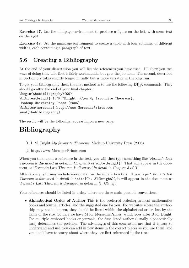
5.6: Creating a Bibliography Writing Mathematics 91
Exercise 47. Use the minipage environment to produce a figure on the left, with some texton the right.
Exercise 48. Use the minipage environment to create a table with four columns, of differentwidths, each containing a paragraph of text.
5.6 Creating a Bibliography
At the end of your dissertation you will list the references you have used. I’ll show you twoways of doing this. The first is fairly workmanlike but gets the job done. The second, describedin Section 5.7 takes slightly longer initially but is more versatile in the long run.
To get your bibliography then, the first method is to use the following LATEX commands. Theyshould go after the end of your final chapter.\beginthebibliography99
\bibitembright I.~M.~Bright. \em My favourite Theorems,
Madeup University Press (2006).
\bibitemmersenne http://www.MersennePrimes.com
\endthebibliography
The result will be the following, appearing on a new page.
Bibliography
[1] I. M. Bright.My favourite Theorems, Madeup University Press (2006).
[2] http://www.MersennePrimes.com
When you talk about a reference in the text, you will then type something like ‘Fermat’s LastTheorem is discussed in detail in Chapter 3 of \citebright’. That will appear in the docu-ment as ‘Fermat’s Last Theorem is discussed in detail in Chapter 3 of [1].
Alternatively, you may include more detail in the square brackets. If you type ‘Fermat’s lastTheorem is discussed in detail in \cite[Ch. 3]bright’, it will appear in the document as‘Fermat’s Last Theorem is discussed in detail in [1, Ch. 3]’.
Your references should be listed in order. There are three main possible conventions.
• Alphabetical Order of Author This is the preferred ordering in most mathematicsbooks and journal articles, and the suggested one for you. For websites where the author-ship may not be known, they should be listed within the alphabetical order, but by thename of the site. So here we have M for MersennePrimes, which goes after B for Bright.For multiple authored books or journals, the first listed author (usually alphabeticallyfirst) determines the position. The advantages of this convention are that it is easy tounderstand and use, you can add in new items in the correct places as you use them, andyou don’t have to worry about where they are first referenced in the text.

92 Writing Mathematics Chapter 5: Dissertations
• Chronological order of publication This is easy to understand, but difficult to finditems, means items by the same author are not necessarily adjacent, and you can get intotrouble with different editions of a book and websites, which are constantly updated sohave no meaningful publication date. The only time where chronological order could comeinto play is if you have several papers or books by the same author. Then alphabeticalorder can’t help you and it is standard practice to put them in chronological order, oldestfirst.
• Order in Which they Appear in the Dissertation Some people like this becauseit seems to make sense that your first reference should be to reference 1, your second toreference 2 and so on. But the main disadvantage is that whenever you rearrange yourtext, which tends to happen quite a lot, you risk changing the order in which you cite yourreferences. So you would need to manually check each time that you haven’t changed theorder. That is asking for trouble! It also means someone looking for a particular nameor book (rather than a number) in the list of references will have a hard time finding it.
You will see that the references are labelled with numbers [1], [2] and so on. If you wouldrather use another system, such as an abbreviated form of the author’s name and the year ofpublication, then you can do this too with an optional argument to \bibitem. So, for example,
\bibitem[BR06]bright I.~M.~Bright.\em My favourite Theorems,
Madeup University Press (2006).
produces [BR06] instead of [1] for the label of the item, and when it is cited in the text with\citebright the reference will be to [BR06].
Bibliography items should be written consistently. For a book, give the authors first, then thetitle in italics, including edition number if relevant, then the publisher and finally the year ofpublication in brackets. For a journal article, give the authors, then title, then journal title(using standard abbreviations such as J. Algebra for ‘Journal of Algebra’), then the volume,number and pages on which the article appeared, followed finally by the year of publication.With e-journals usually the number of pages is listed rather than a start and end page. If youcite any websites you should be as specific as you can with the URL, name of author if known,but of course there is no publication year.
Example 5.4. Here is the bibliography from Sarah Hart’s PhD thesis, as an example. Notethat if you produce a bibliography in the article document class, rather than in book orreport, it will call it ‘References’, rather than ‘Bibliography’.
[1]. N. Bourbaki. Groupes et Algèbres de Lie, Chapitres IV, V and VI, Masson, Paris (1981).
[2]. B. Brink and R.B. Howlett. A finiteness property and an automatic structure for Coxetergroups, Math. Ann. 296, 179–190 (1993).
[3]. B. Brink. The Set of Dominance Minimal Roots, School of Mathematics and Statistics,University of Sydney, Preprint (1995).

5.6: Creating a Bibliography Writing Mathematics 93
[4]. R.W. Carter. Conjugacy Classes in the Weyl Group, Compositio. Math. 25, 1–59 (1972).
[5]. R.W. Carter. Simple Groups of Lie Type, Wiley Interscience (1972).
[6]. A.M. Cohen. Recent Results on Coxeter Groups, for ASI on Polytopes, 18 pages (1993).
[7]. H.S.M. Coxeter. Discrete Groups generated by reflections, Ann. of Math. 35, 588–621(1934).
[8]. H.S.M. Coxeter. The Complete Enumeration of finite groups of the form R2i = (RiRj)
kij
= 1, J. London Math. Soc. 10, 21–25, (1935).
[9]. H.S.M. Coxeter and W.O.J. Moser. Generators and Relations for Discrete Groups,Springer-Verlag, Fourth Edition (1980).
[10]. V.V. Deodhar. On the Root System of a Coxeter Group, Comm. Algebra 10(6) 611–630(1982).
[11]. M. Dyer. Reflection Subgroups of Coxeter Systems, J. Algebra 135, 57–73 (1990).
[12]. D.B. Epstein et al. Word Processing in Groups, Jones and Bartlett, Boston (1992).
[13]. M. Geck and G. Pfeiffer. On the Irreducible Characters of Hecke Algebras, Adv. in Math.102, 79–94 (1993).
[14]. M. Geck, S.Kim and G. Pfeiffer. Minimal Length Elements in Twisted Conjugacy Classesof Finite Coxeter Groups, to appear in J. Algebra.
[15]. R.B. Howlett, P.J. Rowley and D.E. Taylor. On Outer Automorphism Groups of CoxeterGroups, Manchester Centre for Pure Mathematics Preprint (1996).
[16]. J.E. Humphreys. Reflection Groups and Coxeter Groups, Cambridge studies in advancedmathematics, 29 (1990).
[17]. D.L.Johnson. Word Growth of Coxeter Groups, LMS Lecture Note Series 252 ‘Geometryand Cohomology in Group Theory’, 188–189 (1998).
[18]. I.G. Macdonald. The Poincaré Series of a Coxeter Group, Math. Ann. 199, 161–174(1972).
[19]. R.W. Richardson. Conjugacy Classes of Involutions in Coxeter Groups, Bull. Austral.Math. Soc. 26, 1–15 (1982).
Exercise 49. Create a bibliography of three items in your practice dissertation (either one).Cite page 5 of the first item, Theorem 2 of the second and Section 4 of the third.

94 Writing Mathematics Chapter 5: Dissertations
The advantages of creating a bibliography in this way are that it’s easy, you don’t need aseparate file (as the method in Section 5.7 does), and you have complete control over theformatting. The disadvantages are that when you add new items you need to insert themin the correct place, getting your alphabetical ordering (or whatever) correct, it’s easy to beinconsistent about whether you use initials or full names, and that if you decide to changethe order from chronological to alphabetical or vice versa it is very time-consuming. Also,housekeeping like removing references you once needed but now don’t, has to be done manually.If only there was a way of automating some of this. . ..
5.7 Using BibTeX to Manage Your Bibliography
A convenient way of managing your references is through the use of BibTeX. This involvescollecting all your references in a .bib file that is separate from your main .tex file. BibTeXthen allows you to automatically create a bibliography through a simple command. There areseveral advantages to this approach:
• You can collect together references for as many resources as you like because only theones that you cite directly will appear in the bibliography.
• This means if you are writing more than one document on a particular topic you onlyneed to create a single .bib file, because it can be used to create appropriate bibilographiesfor each separate documents if required.
• Many journal websites and resources such as dblp allow you to export references for papersdirectly in the required format, making it easier to create the .bib file.
• By changing a single command you can change the formatting of your bibliography (forinstance you could switch it from being in alphabetical order to being in order of citation).
Creating the .bib file
You can create your .bib file using TEXStudio. Open a blank document and save it asmybibliography.bib (or similar). Now you need to include an entry for each reference. (Theorder in which you create these entries does not matter.) The precise formatting depends onthe nature of the reference: available BibTeX options include:
• article
• book
• inbook (used when referencing a single chapter, for example)
• inproceedings (used for conference papers)
• mastersthesis
• misc (for references that don’t fit the other options)

5.7: Using BibTeX to Manage Your Bibliography Writing Mathematics 95
• phdthesis
• techreport
The following is an example of how you would create a BibTeX entry for an article:
@articlessandrs,
author = Robert J. McEliece and
Dilip V. Sarwate,
title = On Sharing Secrets and Reed-Solomon Codes,
journal = Commun. ACM,
volume = 24,
number = 9,
pages = 583--584,
year = 1981
It includes fields for all the essential information. To cite this reference from within a documentyou would use the command
\citessandrs.
Note that the authors’ first names have been included in the entry here. If we decide laterthat we only want initials to be used in our bibliography we do not have to change the .bibfile, BibTeX can adjust this automatically with a different choice of bibliography style (SeeSection 5.7). One other point to note is that all titles will appear in the bibliography withthe words after the first word all beginning with lower case letters. In this example, we wantthe words “Reed-Solomon” to be capitalised, since they are names. By placing the parenthesesaround the R and the S we can ensure they appear as capitals in the final bibliography.
The various different types of entries have slightly different fields. Here is an example of a book
entry:
@booklidl,
author = R.~Lidl and H.~Niederreiter,
title = Finite Fields,
year = 1997,
edition = 2nd,
isbn = 0-521-39231-4,
series = Encyclopedia of Mathematics and its applications,
Volume = 20,
publisher = Cambridge University Press,
address = Cambridge, UK,
Details for all of the available options for each type can easily be found online.

96 Writing Mathematics Chapter 5: Dissertations
Finding BibTeX Entries Online
Often it is possible to obtain suitably formatted BibTeX entries online, from journal websites,databases or similar. For example, suppose I wish to include an entry for the article “PracticalMinimalist Cryptography for RFID Privacy” that appeared in the IEEE systems journal. Thisarticle appears on the journal’s website at http://dx.doi.org/10.1109/JSYST.2007.907683.When I visit this website, I see there is a “download citations” link on the left of the page. IfI click on the link and select the BibTeX option, it opens a new window with the appropriateentry that I can simply cut and paste into my .bib file:
@ARTICLE4378547,
author=Langheinrich, M. and Marti, R.,
journal=Systems Journal, IEEE,
title=Practical Minimalist Cryptography for RFID Privacy,
year=2007,
volume=1,
number=2,
pages=115-128,
keywords=cryptography;radiofrequency identification;RFID privacy;practical
minimalist cryptography;radio frequency identification;secret sharing;
Assembly;Cryptography;Intrusion detection;Jamming;Performance analysis;
Privacy;Proposals;Protection;RFID tags;Radiofrequency identification;
Minimalist cryptography;Shamir;privacy;radio frequency identification
(RFID);secret sharing,
doi=10.1109/JSYST.2007.907683,
ISSN=1932-8184,
month=Dec,
This is a convenient way of obtaining the details for each reference, but it is wise to check forerrors afterwards. For example, in the above entry I will want to replace the “RFID” in the titleby “RFID” to ensure that the acronym RFID remains in capitals when displayed inthe bibliography.
Creating the Bibliography
First, ensure that your .bib file is placed in the same folder as the .tex file for your document.There are two commands required to create a bibliography for a document using BibTeX. Thefirst is the \bibliographystyle command, which should be placed in the preamble of yourdocument (before the \begindocument)
\bibliographystyleabbrv
This command controls the formatting of your bibliography. The abbrv style results in abibliography that is ordered by the first author’s surname, and in which the authors’ initialsare used in place of first names. Other popular options include:
• unsrt (Items appear [1], [2], etc in the order in which they are cited in your documentwith full first names included if you have provided them.)

5.7: Using BibTeX to Manage Your Bibliography Writing Mathematics 97
• plain (Items are ordered alphabetically by first authors’ surname, full first names aregiven if provided.)
• alpha (Items are ordered alphabetically by first authors’ surname, full first names aregiven if provided, and the citations are not [1], [2] etc but made of the surnames and yearof publication.)
The second is the \bibliography command which is placed where you want the bibliographyto appear (usually at the end of the document).
\bibliographymybibliography
When you compile your document, it should now create the bibliography automatically. Sup-pose the file mybibliography.bib contains the three entries given above and in my document I citejust the first two, in the sentence This document uses \citessandrs and \citelidl.
The numbering and bibliography will appear different for each of the different bibliographystyles. For \bibliographystyleabbrv we’ll get the following:
This document uses [2] and [1].
Bibliography
[1] R. Lidl and H. Niederreiter. Finite Fields, volume 20 of Encyclopedia ofMathematics and its applications. Cambridge University Press, Cambridge,UK, 2nd edition, 1997.
[2] R. J. McEliece and D. V. Sarwate. On sharing secrets and Reed-Solomoncodes. Commun. ACM, 24(9):583–584, 1981.
2
With =\bibliographystyleplain we’ll get full first names where given:
This document uses [2] and [1].
Bibliography
[1] R. Lidl and H. Niederreiter. Finite Fields, volume 20 of Encyclopedia ofMathematics and its applications. Cambridge University Press, Cambridge,UK, 2nd edition, 1997.
[2] Robert J. McEliece and Dilip V. Sarwate. On sharing secrets and Reed-Solomon codes. Commun. ACM, 24(9):583–584, 1981.
2
Using \bibliographystyleunsrt changes the order of references:
This document uses [1] and [2].
Bibliography
[1] Robert J. McEliece and Dilip V. Sarwate. On sharing secrets and Reed-Solomon codes. Commun. ACM, 24(9):583–584, 1981.
[2] R. Lidl and H. Niederreiter. Finite Fields, volume 20 of Encyclopedia ofMathematics and its applications. Cambridge University Press, Cambridge,UK, 2nd edition, 1997.
2
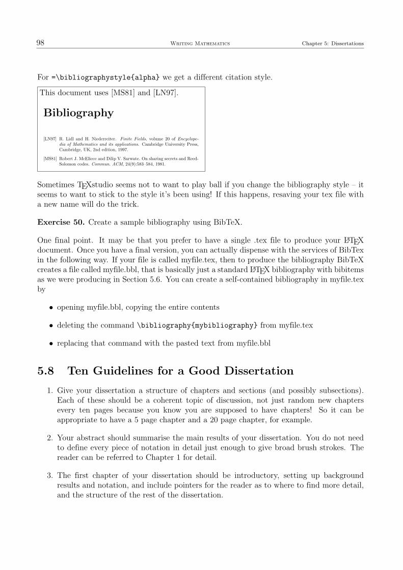
98 Writing Mathematics Chapter 5: Dissertations
For =\bibliographystylealpha we get a different citation style.
This document uses [MS81] and [LN97].
Bibliography
[LN97] R. Lidl and H. Niederreiter. Finite Fields, volume 20 of Encyclope-dia of Mathematics and its applications. Cambridge University Press,Cambridge, UK, 2nd edition, 1997.
[MS81] Robert J. McEliece and Dilip V. Sarwate. On sharing secrets and Reed-Solomon codes. Commun. ACM, 24(9):583–584, 1981.
2
Sometimes TEXstudio seems not to want to play ball if you change the bibliography style – itseems to want to stick to the style it’s been using! If this happens, resaving your tex file witha new name will do the trick.
Exercise 50. Create a sample bibliography using BibTeX.
One final point. It may be that you prefer to have a single .tex file to produce your LATEXdocument. Once you have a final version, you can actually dispense with the services of BibTexin the following way. If your file is called myfile.tex, then to produce the bibliography BibTeXcreates a file called myfile.bbl, that is basically just a standard LATEX bibliography with bibitemsas we were producing in Section 5.6. You can create a self-contained bibliography in myfile.texby
• opening myfile.bbl, copying the entire contents
• deleting the command \bibliographymybibliography from myfile.tex
• replacing that command with the pasted text from myfile.bbl
5.8 Ten Guidelines for a Good Dissertation
1. Give your dissertation a structure of chapters and sections (and possibly subsections).Each of these should be a coherent topic of discussion, not just random new chaptersevery ten pages because you know you are supposed to have chapters! So it can beappropriate to have a 5 page chapter and a 20 page chapter, for example.
2. Your abstract should summarise the main results of your dissertation. You do not needto define every piece of notation in detail just enough to give broad brush strokes. Thereader can be referred to Chapter 1 for detail.
3. The first chapter of your dissertation should be introductory, setting up backgroundresults and notation, and include pointers for the reader as to where to find more detail,and the structure of the rest of the dissertation.

5.8: Ten Guidelines for a Good Dissertation Writing Mathematics 99
4. You may assume that the reader has an undergraduate knowledge of mathematics. It issensible to establish your terminology in any case, for example whether your functionswill act on the right or the left, or any conventions for your dissertation such as thatG will always be a finite group. Any notation not commonly used in undergraduatemathematics should be carefully defined and used consistently.
5. You must be sure to include plenty of examples, wherever possible examples that youhave invented yourself. It helps the reader to confirm that they have understood whatyou are saying. It shows that you are doing original work, not just writing down a lot oftheorems from books. It also means that if there is a slip somewhere in a definition, likea missing minus sign, its correct use in an example will show the examiners that the slipwas just a slip, and not an error of understanding on your part.
6. When you reintroduce a topic after several pages, it is sensible and kind to remind thereader what all the symbols mean. So you could say something like ‘recall that Hα is thehyperplane orthogonal to α, as defined in Section 1.4’. Similarly, in a proof, don’t justsay ‘by Lemma 2.3, the group G is cyclic’. The reader doesn’t remember what Lemma2.3 said! Remind us: ‘Lemma 2.3 showed that any finite subgroup of the multiplicativegroup of a field is cyclic. Therefore G is cyclic’.
7. Take the trouble to display equations and to break text up into paragraphs. It is mucheasier to read well laid-out text than to struggle through streams of consciousness.
8. Use simple, clear language.
9. Include a bibliography. Do not pad it out with items that you have not cited — thisis unhelpful and misleading. Label and describe the items clearly and consistently, forexample by putting them in alphabetical order.
10. When using a reference, always cite it properly, and include guidance as to where in thereference to look. If you state a theorem and then say that the proof is in [3], when [3] isa 600 page book, it’s not very helpful! Much better to say that the theorem is proved asProposition 4.6 of [3].