I /

WRDC-TR-89-4072

CARBON FIBER MORPHOLOGY: WIDE-ANGLEX-RAY STUDIES OF PITCH- AND PAN-BASZDCARBON FIBERS

Dr. David P. Anderson

University of Dayton Research Institute

300 College Park AvenueDayton, OH 45469-0001

July 1989

N Interim Report for Period January 1988 - December 1988

mi DTICE LCTEOCT 3 01989 U

Approved for public release; distribution unlimited.

MATERIALS LABORATORYWRIGHT RESEARCH AND DEVELOPMENT CENTERAIR FORCE SYSTEMS COMMANDWRIGHT-PATTERSON AIR FORCE BASE, OHIO 45433-6533

89 10 27 192

NOTICE

When Government drawings, specifications, or other data are used forany purpose other than in connection with a definitely Government-relatedprocurement, the United States Government incurs no responsibility or anyobligation whatsoever. The fact that the Government may have formulated orin any way supplied the said drawings, specifications, or other data, is notto be regarded by implication, or otherwise in any manner construed, aslicensing the holder, or any other person or corporation; or as conveyingany rights or permission to manufacture, use, or sell any patented inventionthat may in any way be related thereto.

This report is releasable to the National Technical Information Service(NTIS). At NTIS, it will be available to the general public, including for-eign nations.

This technical report has been reviewed and is approved for publica-tion.

MARVTIN KNIGHT, Project E;'ineerMechanics & Surface Inte *ctions BrNonmetallic Materials Division

FOR THE COMMANDER 'II

MOUEILL L. MINGESDirectorNonmetallic Materials Division

If your address has changed, if you wish to be removed from our mailinglist, or if the addressee is no longer employed by your organization, pleasenotify WRDC/MIBM, Wright-Patterson AFB, OH 45433-6533 to help maintain acurrent mailing list.

Copies of this report should not be returned unless return is required bysecurity considerations, contractual obligations, or notice on a specificdocument.

UNCLASSIFIEDSECURITY CLASSIFICATION OF THIS PAGE

Form ApprovedREPORT DOCUMENTATION PAGE OMB No. 0704-0188

la. REPORT SECURITY CLASSIFICATION lb. RESTRICTIVE MARKINGS

Unclassified2a. SECURITY CLASSIFICATION AUTHORITY 3. DISTRIBUTION /AVAILABILITY OF REPORT

Approved for public release; distribution2b. DECLASSIFICATION/'DOWNGRADING SCHEDULE Unl imited.

4. PERFORMING ORGANIZATION REPORT NUMBER(S) 5. MONITORING ORGANIZATION REPORT NUMBER(S)

UDR-TR-89-61 WRDC-TR-89-4072

6a. NAME OF PERFORMING ORGANIZATION 6b. OFFICE SYMBOL 7a. NAME OF MONITORING ORGANIZATIONUniversity of Dayton (if applicable) Materials Laboratory (WRDC/MLBM)Research Institute Wright Research and Development Center

6c. ADDRESS (City, Stat, and ZIP Code) 7b. ADDRESS (City, State, and ZIP Code)300 College Park Avenue Air Force Systems CommandDayton, OH 45469-0001 Wright-Patterson AFB, OH 45433-6533

Ba. NAME OF FUNDING/SPONSORING 8b. OFFICE SYMBOL 9. PROCUREMENT INSTRUMENT IDENTIFICATION NUMBERRGANITIN .(If applicable)

Materiabs aoratory C F33615-87-C-5239Wright Research & Devel. Cete WRDC/MLBMkc. ADDRESS (City, State, and ZIP Code) 10. SOURCE OF FUNDING NUMBERSAir Force Systems Command PROGRAM PROJECT TASK WORK UNIT

Wright-Patterson AFB, OH 45433-6533 ELEMENT NO. NO. NO ACCESSION NO.62102F 2419 02 25

11. TITLE (Include Security Classification)

CARBON FIBER MORPHOLOGY: WIDE-ANGLE X-RAY STUDIES OF PITCH- AND PAN-BASED CARBON FIBERS

12. PERSONAL AUTHOR(S)Dr. David P. Anderson

13a. TYPE OF REPORT 13b. TIME COVERED 14. DATE OF REPORT (Year, Month, Day) 15. PAGE COUNTInterim FROM Jan 88 ToDec 88 July 1989 119

16. SUPPLEMENTARY NOTATION

17. COSATI CODES 18. SUBJECT TERMS (Continue on reverse If necessary and identify by block number)FIELD GROUP I SUB-GROUP carbon fiber- graphite fiber- x-ray diffraction11 04 1 crystals, graphitization .-

11 1 07 1 crystallite size, orientation19. ABSTRACT (Continue on reverse if necessary and identify by block number)

A This report describes the wide-angle x-ray diffraction techniques used to examinecarbon and graphite fibers and the results of several fibers. A series of commercialPAN- and pitch-based carbon fibers whose tensile moduli spanned the generally availablerange were examined. Crystal perfection, size, orientation, and degree of graphitizati6ncorrelated well with tensile moduli but less well with tensile and compressive strength.

20. DISTRIBUTION /AVAILABILITY OF ABSTRACT 21. ABSTRACT SECURITY CLASSIFICATIONrUNCLASSIFIEDIUNLIMITED 03 SAME AS RPT. 0 DTIC USERS Unclassified

22a. NAME OF RESPONSIBLE INDIVIDUAL 22b. TELEPHONE (Include Area Code) 22c. OFFICE SYMBOLMarvin Kni ht (513)2-7131 WRDC/MLBMD Form 1473, JUN 86 Previous editions are obsolete. SECURITY CLASSIFICATION OF THIS PAGE

UNCLASSIFIED

FOREWORD

This Interim Technical Report was prepared by the Universityof Dayton Research Institute, 300 College Park Avenue, Dayton, OH45469-0001, under Air Force Contract No. F33615-87-C-5239. Itwas administered under the direction of the Materials Laboratory,Wright Research and Development Center, Air Force SystemsCommand, Wright-Patterson Air Force Base, OH, with Mr. MarvinKnight (WRDC/MLBM) as the Project Engineer.

The use of commercial names of materials in this report isincluded for completeness and ease of scientific comparison only.It in no way constitutes an endorsement of these materials ormanufacturers.

This report covers work conducted from January throughDecember 1988.

L IiU , ...' , .-- , , .

Drc J I;TC, ............. .

INyPECrE By

Dist

iii

ACKNOWLEDGEMENTS

The author would like to thank Dr. Satish Kumar of UDRI and'.specially Major Joseph Hager of WRDC/MLBC for comments andriticisms on this report during its assembly.

TABLE OF CONTENTS

SECTION PAGE

1 INTRODUCTION 1

2 NOMENCLATURE 3

2.1 Hexagonal Indexing 3

2.2 Diffractometer 6

2.3 Fiber Diffraction 11

3 CARBON/GRAPHITE REFLECTIONS 19

3.1 Graphite Crystals 19

3.2 Two-Dimensional Lattices 253.3 Crystallite Sizes 26

3.4 Misorientation 33

4 RESULTS 40

4.1 Materials 40

4.2 (00,2) Results 40

4.3 Advanced Lc Results 45

4.4 3-D and La Results 51

4.5 Other 66

5 CONCLUSIONS 67

REFERENCES 68

APPENDIX A: Flat-Film WAXD Photographs ofCarbon Fibers 71

APPENDIX B: Diffraction Scans (Chi=700 ) ofthe (10) and (10,1) Region ofthe Carbon Fibers 79

APPENDIX C: Diffraction Scans (Chi=70° ) ofthe (11) and (11,2) Region ofthe Carbon Fibers 95

v

LIST OF ILLUSTRATIONS

FIGURE PAGE

1 Hexagonal Axes and Crystal Planes in the GraphiteBasal Plane 4

2 Diagrams of Planes Having Various Miller Indicesin an Orthorhombic Unit Cell With Edges a, b, andc 5

3 Bragg's Law Diffraction 7

4 Schematic of X-ray Flat-Film Camera (Sl, S2, and

S3 are the camera's collimator) 9

5 Flat-Film WAXD Photograph of P-100 Carbon Fiber 9

6 Four-Circle Diffractometer Geometry With a FiberSample 10

7 Equatorial Diffraction Geometry 12

8 Meridional Diffraction Geometry 14

9 Cone Defined by Fiber Off-Axis Plane Normals 15

10 Off-Axis Diffraction Geometry - Omega CircleAdjustments 16

11 Off-Axis Diffraction Geometry - Chi CircleAdjustments 17

12 Comparison of Turbostratic and 3-D GraphiteCrystals in Carbon Fibers 20

13 The Entwined Fibrils Model of Carbon FiberMorphology of Diefendorf and Tokarsky 22

14 The Wavy Fibrils Model of Carbon Fiber Morphologyof Perret et al. 22

15 The Thumb-Print Cross-Section Model of Carbon FiberMorphology of Bacon 23

16 The Holey Curved Bundles of Graphite Sheets Modelof Carbon Fiber Morphology of Barnet and Noor 23

17 The Holey Curved Bundles of Graphite Sheets Modelof Carbon Fiber Morphology of Bennett and Johnson 24

vi

LIST OF ILLUSTRATIONS (Continued)

FIGURE PAGE

18 Theoretical Intensity Profiles of the 2-D Graphite(11) Peak from Randomly Oriented Crystals ofSeveral Sizes 27

19 Intensity Distribution from 2-D Crystal SheetsOriented Parallel to the Fiber Axis 28

20 Comparison Between Gaussian and CauchyDistributions 30

21 Curve-Fit Beryllium Acetate Diffraction Scan Usedto Measure Instrumental Broadening Effects 32

22 Theoretical (00,2) Reflection With and WithoutInstrumental Broadening Folded in for Lc = 1OOA 34

23 Theoretical Asymmetric 2-D Profile With andWithout Instrumental Broadening Folded in forLa = 100A 35

24 Typical Fiber Sample Bundles: a) Mounted WithTape at Fiber Ends and b) Mounted in Cyanomethyl-acrylate Glue 36

25 Plots of (00,2) Azimuthal Distributions for P-25and P-100 Carbon Fibers 38

26 Curve-Fit (00,2) Bragg Reflection of P-55 43

27 Curve-Fit (00,2) Azimuthal Scan of P-55 44

28 Complete Equatorial Bragg Scan of P-100 46

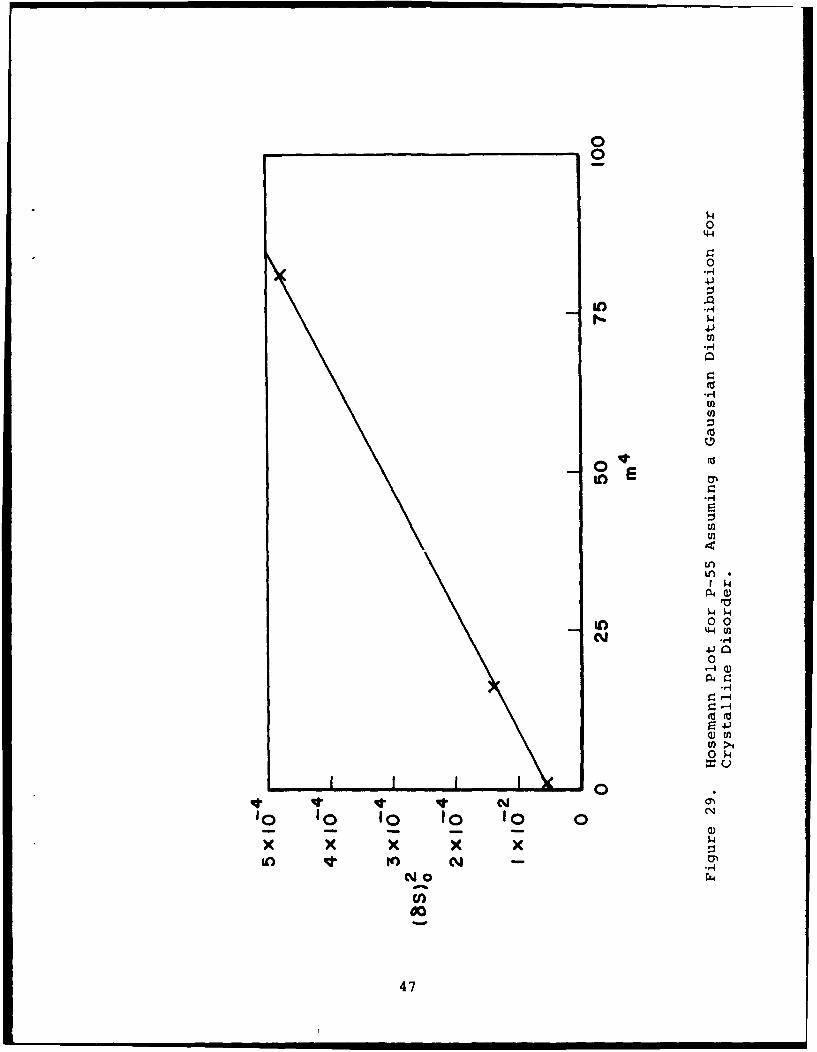
29 Hosemann Plot for P-55 Assuminq a GaussianDistribution for Crystalline Disorder 47

30 Hosemann Plot for P-55 Assuming a CauchyDistribution for Crystalline Disorder 48

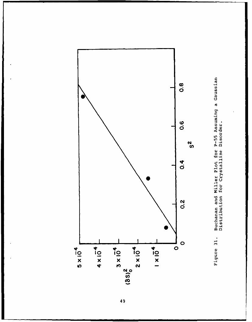
31 Buchanan and Miller Plot for P-55 Assuming aGaussian Distribution for Crystalline Disorder 49

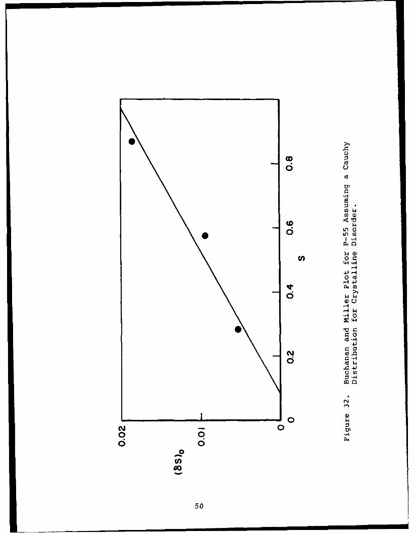
32 Buchanan and Miller Plot for P-55 Assuming aCauchy Distribution for Crystalline Disorder 50

33 P-100 Diffraction Showing the Emergence of the(10,1) Off-Axis Reflection by Fiber Tilting 55

vii

LIST OF ILLUSTRATIONS (Concluded)

FIGURE PAGE

34 Complete Meridional (Chi=900) Bragg Scan of P-100 57

35 Complete Off-Axis (Chi=70° ) Bragg Scan of P-100 58

36 Bragg Scan of (10,1) Region in Some PiLch-BasedFibers 59

37 Bragg Scan of (11,2) Region in Some Pitch-BasedFibers 60

38 Bragg Scan of (10,1) Region in Some PAN-BasedFibers 61

39 Bragg Scan of (11,2) Regiork in Some PAN-BasedFibers 62

viii

LIST OF TABLES

TABLE PAGE

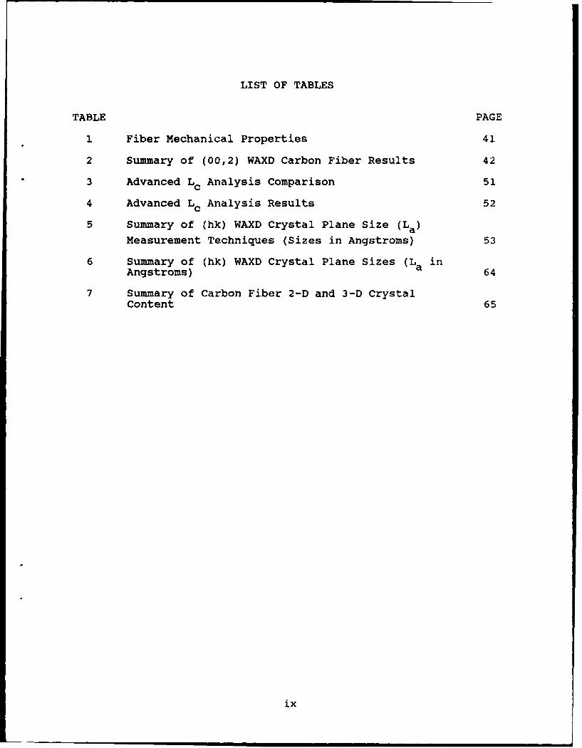
1 Fiber Mechanical Properties 41

2 Summary of (00,2) WAXD Carbon Fiber Results 42

3 Advanced Lc Analysis Comparison 51

4 Advanced Lc Analysis Results 52

5 Summary of (hk) WAXD Crystal Plane Size (La)

Measurement Techniques (Sizes in Angstroms) 53

6 Summary of (hk) WAXD Crystal Plane Sizes (La inAngstroms) 64

7 Summary of Carbon Fiber 2-D and 3-D CrystalContent 65

ix

1. INTRODUCTION

Carbon fibers are extremely important components in high

performance composites as they are the primary reinforcingmaterial. Because the mechanical properties of fibers aredependent on their structures, the structure of carbon fibers hasbeen examined by many researchers [1-13]. A continued interest

in this area results from the emergence of new carbon fibers with

improved properties.

Pitch-based fibers traditionally had high stiffnesses buthad weak tensile strengths. PAN-based fibers were strong butlacked high moduli. Recent developments have improved these

fibers' properties, and more work is focusing on the compressiveproperties as well. These property changes result from struc-tural differences created during the fiber manufacture.

Several diffraction techniques have been used to examine thecrystalline microstructure of carbon fibers. Wide-angle x-raydiffraction (WAXD), as its name implies, uses the diffraction ofx-rays to examine the basic crystalline structure at scatteringangles in excess of several degrees (i.e. >50). Structures about

the size of crystalline interplanar spacings (1 to 15A) arestudied. Small-angle x-ray scattering (SAXS), on the other hand,examines the scattering of x-rays at lower angles. In SAXSlarger structures, such as crystallites, are examined (sizes up

to several 1000A). Both x-ray methods examine relatively large

volume (1 mm 3), bulk properties. Smaller sample volumes can beexamined using selected area diffraction (SAD) which uses scat-tering of electrons to examined structures which are comparablein size to those in WAXD but using much smaller sample volumes(0.1 Am 3). SAD also has the advantage of being used in conjunc-tion with transmission electron microscopy (TEM) so that imagesof the diffracting area may be obtained (but of course also has

the complex sample preparation difficulties of TEM).

WAXD has been used to examine carbon fibers [1-3,14] interms of the basic graphitic-like crystals present. This tech-nique is now usually used only to quantify specific propertiessuch as graphite plane orientation and degree of graphitization.In this study some of the newer fibers were examined with WAXD,and some interesting and heretofore unreported properties of thecrystalline nature of carbon fibers were discovered.

Most of the publications on x-ray diffraction of carbonfibers are either aimed at experts or only use this technique ina minor role. For this reason significant space in this reportis devoted to explaining the terms and notations used in WAXD.

2

2. NOMENCLATURE

2.1 HEXAGONAL INDEXING

Carbon fibers have a graphite-like crystal nature. Graphite

unit cell is hexagonal corresponding to the hexagonal grid of the

basal plane structure. In Figure 1 the hexagonal grid represents

the aromatic C-C bonds in the basal plane sheets; a carbon atom

is located at each grid vertex.

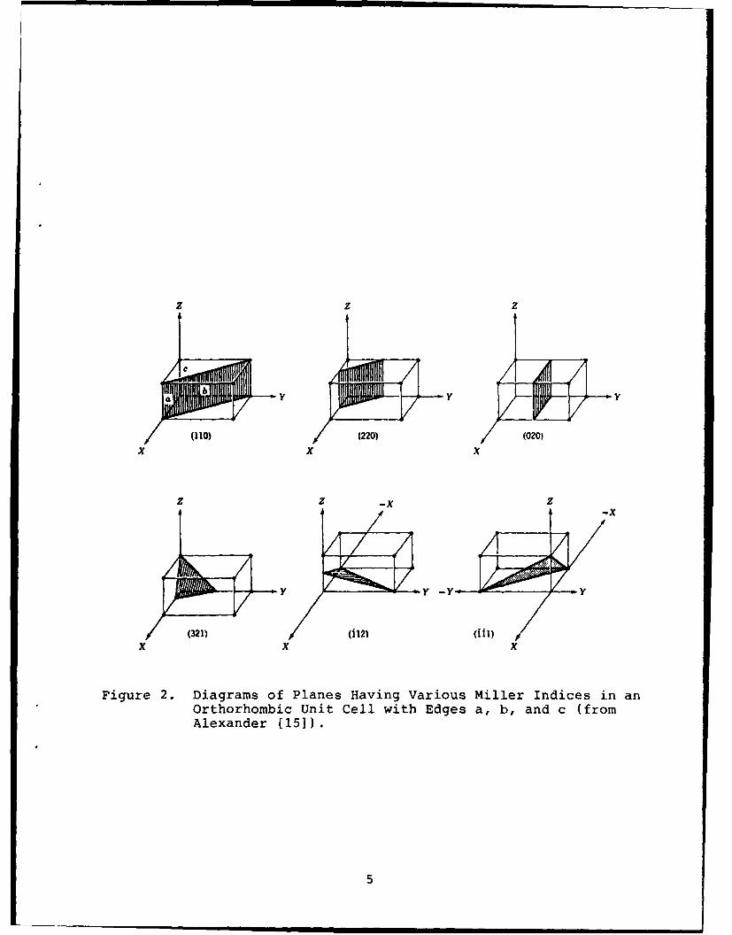
Conventional Miller's indices for crystals consist of three

numbers: h, k, and 1 written as (hkl). These numbers equal the

reciprocal value of where the designated plane cuts the unit cell

boundaries along the x-, y-, and z-axes respectively. Thus an

index set of (210) describes a plane which is parallel to the

z-axis and cuts the unit cell at a/2 and b/l (a, b, and c are the

dimensions of the unit cell along respective axes). Planes that

intersect the unit cell on a negative axis have a bar over them

(e.g., 111). For orthorhombic unit cells, a, b, c are different

but all at right angles which resemble a rectangular box. Figure

2 shows several examples of planes defined by their Miller's

indices.

The literature shows several ways in which the graphitic

planes of carbon and graphite fibers are described by Miller

indices:

h(hk) ( hkil) (hk.l)

(10) (100) (1010) (10,0)

(11) (110) (i120) (11,0)

(002) (0002) (00,2)

(112) (1122) (11,2)

In hexagonal crystals, such as graphite, the angle betweenthe a- and b-axes is 1200. Here, three axes of symmetry of which

two are arbitrarily assigned as unit cell axes in the three index

3

10 or o 1,0)

(,o~o (,o~o 1.3 A

Figure 1. Hexagonal Axes and Crystal Planes in the Graphite BasalPlane.

4

z z z

C

y YY

(220) (020)Sx x

z z -X z

y y -

(321) |2 |1

X x

Figure 2. Diagrams of Planes Having Various Miller Indices in anOrthorhombic Unit Cell with Edges a, b, and c (fromAlexander (15]).

5

systems are given above or all three assigned as in the four in-

dex system. Figure 1 shows these unit cell axes as well as the

example (hk,o) crystal plane projections from the first two rows

above (the crystal planes are perpendicular to the diagrammed

plane). Recognize that because the a and b axes are arbitrarily

assigned, there are equivalent planes at ±1200 from those

diagrammed. The c-axis is perpendicular to the graphite basal

plane so that the (00,2) crystal planes coincide with the basal

planes.

The first column listed actually refers to single graphitic

sheets, as these 2-D crystals require only two indices; these are

important in carbon fibers as will be explained later. The

second and fourth columns are abbreviations of the third column

in hexagonal indices. The second column, while used extensively

in the literature, does not convey the hexagonal nature of the

crystals (versus orthorhombic for example) to the reader as do

the last two columns. The third column is the typical hexagonal

indices which includes a third in-plane index defined such that

the first three indices always sum to zero. Since that third

in-plane index is defined by the first two, it is unnecessary;thus the last column line fully defines the crystal planes and

conveys their hexagonal nature.

The advantage of column three over four is the ability tospot equivalent planes from the indices. Generally in graphite

one refers to only one set of indices when discussing that family

of equivalent planes, negating that advantage. As a matter of

convenience, the indices as shown in the last column will be used

in the report.

2.2 DIFFRACTOMETER

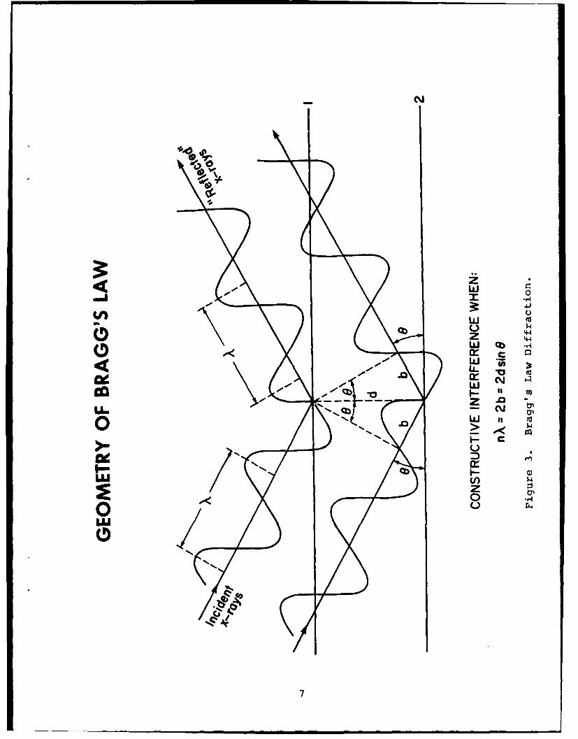
For any crystalline plane to appear in WAXD, it must meet

the Bragg conditions (see Figure 3). This means that the crystal

plane normal must lie in the x-ray collection plane (plane con-taining the incident beam and diffracted ray detector) and

bisects the incident and diffracted rays. To understand this one

6

N

4J

Rs

\U

4-4

W- C4w

LL.cu

LLICX/

N?

must first understand the multiple "geometries" of the data col-

lection system, the sample, the crystals within the sample, and

crystal planes within the crystals.

There are two typical types of data collection: flat-film

and diffractometer. In the flat-film technique, a fiber bundle

is placed directly in front of the collimators (metal tubes with

small holes in either end that only allow parallel beams of

x-rays to pass), and a flat film pack is placed on the other side

perpendicular to the x-ray main-beam and parallel to the fiber

bundle (see Figure 4). The sample-to-film distances are typi-

cally 29 or 50 mm for WAXD and much longer (e.g. 290 mm) for

SAXS. The upper limit of diffraction angle accessible in flat-

film photos is about 500 20. Figure 5 is a typical flat-film

photo of a carbon fiber. Appendix A contains flat-film photo-graphs of the commercially available fibers examined.

The diffractometer is much more general in its sample posi-

tioning and data collection precision. The main x-ray beam is

collimated to hit the center of a 4-circle sample holder; the

detector is in the horizontal plane pivoting about the center of

the sample holder. Figure 6 shows the rotations available in the

sample holder of a 4-circle diffractometer (this diffractometer

is basically a computer-controlled 4-axis sample holder) relative

to a fiber sample. The sample holder is rotated one half the

scattering angle of the detector in the so-called 0-28 collection

geometry; these rotations are the first and second circles. You

may wish the sample to be other than this simple arrangement, andthe second circle (omega) allows one to deviate from the 0-20

condition but still keep the rotation about a vertical line.

Note that some machines define omega as the total angle the

sample plane moves or theta plus omega by the current definition.

The azimuthal circle (chi) tilts the sample in the vertical plane

defined by the first two circles. The last circle (phi) is a

rotation of the sample about its base as defined by the first

three circles. (Note that if chi=0 ° , then phi rotation is the

same as an omega rotation.)

8

I!Meridian

Fiberaxis Film t

P

' _. Equator

Figure 4. Schematic of X-ray Flat-Film Camera (Sr S2' and S3are the camera's collimator)(from Alexander [15]).

(10,1)

(10,1) Satellite

(00,2)

(10,0)

Amorphous Glue

Halo

Figure 5. Flat-Film WAXD Photograph of P-100 Carbon Fiber.

9

-z40

Zo a

U--

0-N z

< w -oo

'4J

00

44xL R

04.)

4-4

.P4

01

Single crystal diffraction yields spots for each crystalplane which meets the Bragg condition. To measure the intensity

of these spots, the 20 detector scans must be made at sampleorientations of all phi, chi, and omega. The other extreme is

powder samples (or bulk crystallized polymers) which have withintheir sample volume crystals already oriented in all directions.

Powder samples produce rings instead of spots, and thereforesimple Bragg scans are adequate.

Common diffraction scans for powders and polymers includeBragg and azimuthal (or chi) scans. A Bragg scan is when asample's scattering intensity is measured by stepping the detec-tor through 29 (usually in steps of 0.10) while the sample plane

is moved one-half that angle (0-20 collection geometry). Theazimuthal scan is when the scattering intensity is measured byrotating the sample through the chi circle (or fraction of the

chi circle since each quadrant is equivalent) with the detectorat a fixed Bragg angle. In both scans phi and omega may be fixedat any desired position.

2.3 FIBER DIFFRACTION

Fibers in general and carbon fibers specifically are axiallysymmetric; that is, a rotation about the fiber axis (phi) does

not change its diffraction pattern. Any axial nonsymmetry inindividual fibers can be averaged out by using a randomlyassembled fiber bundle so that the fiber bundle pattern is

axially symmetric.

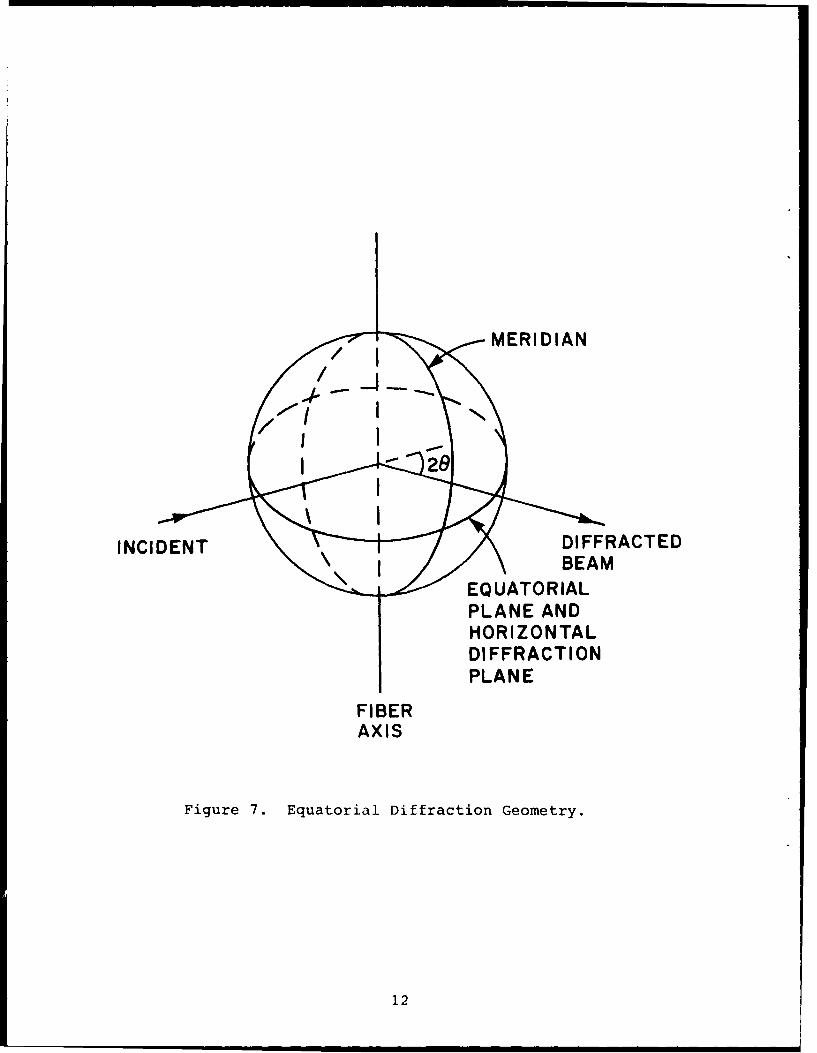
The easiest way of understanding the terminology of fiberdiffraction is to imagine the fiber stretched from pole to poleof a hollow globe. "Equatorial" reflections result from crystal

planes parallel to the fiber axis such that their normals allfall in the sample equatorial plane, and diffraction appears atthe globe's equator with both the main and diffracted beams inthe equatorial plane (chi=0°, see Figure 7). In flat-film photos

the equatorial reflections appear along the horizontal axis whenthe fibers were held vertically (see Figure 4).

11

MERIDIAN

I1 I

INCDN DIFFRACTEDINCIDET \ IBEAM

~EQUATORIAL

PLANE ANDHORIZONTAL

DIFFRACTIONPLANE

FIBERAXIS

Figure 7. Equatorial Diffraction Geometry.

12

"Meridional" reflections are from crystal planes in thefiber that are perpendicular to the fiber axis such that theirnormals are parallel to the fiber axis or pointed to the globe'spoles. These diffraction spots appear on any of the globe'smeridians as the main and diffracted beams occur at the samelatitude on opposite sides of the globe. The fiber must be at

chi=90" to fulfill that condition (see Figure 8). In a flat-film

photo meridional reflections should not be visible, although theysometimes are due to misalignment of the crystals in the fiberwhich will be discussed below.

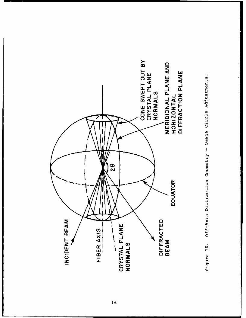
"Off-axis" reflections arise from crystal planes tilted atsome angle other than 900 and 00 to the fiber axis. The planenormals will sweep out a cone at both ends of the globe (seeFigure 9) requiring the fiber to be tilted. In fact the anglethe crystal planes make with the fiber axis (one-half the cone

angle) is the amount of tilt the fiber must make from themeridional conditions to show off-axis reflections. Figure 10

shows the fiber being tilted by an omega rotation, and Figure 11shows a chi rotation (900 minus one-half the cone angle).

The need to tilt the fibers to observe off-axis diffractionwas recognized for Pitch-based carbon fibers in early electrondiffraction SAD studies [16]. The SAD technique looks at a smallsection of the fiber and is very sensitive to local variations inthe crystal alignment. PAN-based fibers of that day showed nooff-axis reflections in either SAD or WAXD. The same rules applyto WAXD except the average misalignment in a fiber bundle isgenerally large enough to generate the required tilt for some ofthe crystals even if the bundle isn't tilted.

Off-axis reflections show up on flat-film photos only when eequals one-half the cone angle (and when misalignment allows the

crystal to fulfill the Bragg condition). The graphite sheets incarbon fibers only lie approximately parallel to the fiber axis(see section 3.1) with varying degrees of misalignment (or tilt-

ing) of those planes away from the fiber axis. In carbon fibersthe (10,1) reflection occurs at 20=44.6 ° , and this plane is

13

z4 wAw z

~Ja.

440-

0Z-04

Q1)

0

.4 4

cN 4-4

0

Z 0w w0

z

ClQ)

4j

w I-

o

14

CONE ANGLE

FIBERAXIS

Figure 9. Cone Defined by Fiber Off-Axis Plane Normals.

15

z

0oz wz4

w cf CL 4-)Z U)

z>c 0 Z(o<

Sz U

4-)

CJD r00

0 H

o 44w 44I

_o 44

< a.

w cn IL 0j-0 w w-

z Li..rn0 -(Z 44

16

hi z

-4-

014-4

4

LLi 0

zU

0 4-4v-4

wU

44

o0I- 0

z a.4-

0 w . -1-t4 0

cr 4 Q)3: J 4

0 -1 U)x a. U)

0 0

z1

O17

tilted 17.60 from the fiber axis; since the difference between

22.3 ° and 17.60 is less than the typical basal plane misalign-

ment, the (10,I) reflection should be visible in flat-film photos

and can be seen in high modulus fibers such as P-100 (see

Appendix A).

Meridional reflections can be seen as special cases of the

general off-axis case; crystal plane tilt is 0° , therefore the

cone angle is zero and diffraction occurs at chi=90 ° and

omega=0 °. Likewise in the equatorial reflections, the crystal

tilt is 900 from the fiber axis in which case the cone has opened

up to 1800 or simply the equatorial plane.

18

3. CARBON/GRAPHITE REFLECTIONS

3.1 GRAPHITE CRYSTALS

In carbon fibers the orientations of the crystalline

graphite planes are approximately parallel to the fiber bundlebut randomly placed within the fiber cross section with thea- and b-axes of the graphite planes randomly oriented. Thus the

(00,1) reflections are equatorial while (hk,O) are usuallyassociated with the meridional region.

The graphite sheets in carbon fibers are by themselves two-dimensional crystals (i.e. the atoms that make up the sheets arein precise locations relative to the other atoms). If these two-dimensional crystalline graphitic sheets are randomly placed withrespect to the next sheet, this is the so-called "turbostratic"structure. In highly graphitized fibers, 3-D crystals are formedwhen the atoms of one sheet are placed in a specific position

relative to the atoms in the next sheet (i.e., in precise crys-tallographic registry). Figure 12 shows a comparison of the

above two cases.

A review by Ruland [17] gives the "best" values for thegraphite crystal dimensions as a = b = 2.4614A, c = 6.707A.

These values are slightly different from the JCPDS [18] valuesfor basal crystalline graphite but not significantly so for most

carbon fiber work (a = b = 2.463A, c = 6.714A). Ruland [17] also

lists an interplane spacing for turbostratic carbon of 3.440A(interplane spacing in crystalline graphite = 3.3535A).

Because the a- and b-axes are randomly oriented with respectto the fiber axis, the (hk,O) plane normals sweep out a completecircle in the sample planes parallel to the fiber; and becausethe fibers are axially symmetric, the normals of all the (hk,0)planes sweep out a complete sphere. Such planes should have aring-like diffraction pattern similar to that for a powder but,in fact, behave like meridional reflections.

The graphite planes in fibers, however, are not large flatsheets. Several models of carbon fiber microstructure are shown

19

FIBER AXIS

(A) (B)

SCHEMATIC DIAGRAMS OF (A) A THREE-DIMENSIONAL GRAPHITE AND(B) A TURBOSTRATIC STRUCTURE

Figure 12. Comparison of Turbostratic and 3-D GraphiteCrystals in Carbon Fibers.

20

here. These include the entwined fibrils observed by Diefendorfand Tokarsky [8] (Figure 13), the wavy fibrils of Perret et al.[1-3] (Figure 14), the thumb-print cross section of Bacon [5)(Figure 15), and the holey curved bundles of graphite sheets ofBarnet and Noor (6,7) (Figure 16) and Bennett and Johnson [9,10](Figure 17). In the fiber axis direction, the ordering of atomsin the (hk,0) planes is sufficient to generate diffraction. Thatis to say that along the fiber, the number of crystal planes issufficiently large enough to produce constructive interference ina Bragg scan. The size of this stack of planes is called thepersistence length.

The average random orientation of the a- and b-axes in thegraphite sheets or bundles is such that all (hk,0) planes thatcan produce diffraction do so in the meridional region. Sheetsor bundles that produce the (10) or (10,0) reflection will notshow the (11) or (11,0) reflection, but other sheets or bundleswill. Also a distribution of orientations within those bundleswill generate diffraction; as one rotates from vertical to hori-zontal, the persistence length along the effective flat areadrops dramatically. Thus the effective size of the (hk) crystalsand number capable of diffracting decrease. From the globe anal-ogy (section 2.2) instead of the probabilities all concentratedat the poles coincident with the fiber bundle, a distribution of

probabilities exist, centered about poles, finite but rapidlydecreasing as one gets further away from the poles. This analogyis also complicated by the change in the crystals sizes and

orientations.

The off-axis (hk,1) plane normals in graphite will sweep outthe cone described in section 2.2 above at each pole. If the

graphite planes were large and flat, they would sweep out anentire sphere minus the cone at the poles. As described in theparagraph above, the (hk,l) reflections also have probabilitiesof diffracting at more than the ring on the globe defined by thecone. Note however that the cone defines the upper limit for theprobabilities with zero probability at latitudes greater and a

decreasing probability at lower latitudes.

21

I AXIAL IIBECTIIN

~L.

La

FlIERSURFACE

Figure 13. The Entwined Fibrils Model of Carbon FiberMorphology of Diefendorf and Tokarsky [81.

Figure 14. The Wavy Fibrils Model of Carbon Fiber Morphology ofPerret etal. [1-3] .

22

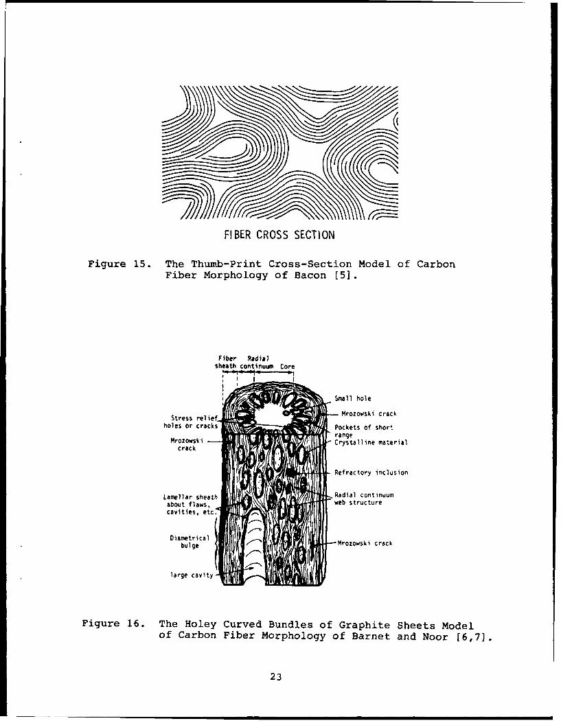
FIBER CROSS SECTION

Figure 15. The Thumb-Print Cross-Section Model of CarbonFiber Morphology of Bacon [5].

Fiber Radio)sheath continuum Core

' Small hole

Stress relie Mrozowski crack

holes Or cracks Pockets of short

Mrozwskirange

crack Crystalline material

Refractory inclusion

Lamellar sheath Radial continuumme'ut f i., -web structureabout flaws,cavities, etc.

Diametrical I

bulge I Mrozowski crack

large cavity-

Figure 16. The Holey Curved Bundles of Graphite Sheets Modelof Carbon Fiber Morphology of Barnet and Noor [6,7].

23

Figure 17. The Holey Curved Bundles of Graphite SheetsModel of Carbon Fiber Morphology of Bennettand Johnson [9,10].

24

3.2 TWO-DIMENSIONAL LATTICES

The dimensionality of the graphitic crystals in carbon fiber

is a source of some controversy - the turbostratic carbon struc-

ture being 2-D and crystalline graphite being 3-D. Carbon fibers

of low modulus <25 Msi being predominantly turbostratic and

gradually increasing to more crystalline graphitic nature as one

goes to higher modulus fibers. The observation of off-axis

reflections is considered necessary proof of 3-D crystals; and

generally only high modulus Pitch based carbon fibers exhibit

these off-axis reflections.

The diffraction from a three-dimensional crystal lattice is

very nearly symmetric. That is, the maximum peak intensity is

very close to the position with equal intensity on both sides

(the peak centroid). This is true whether the intensity is

plotted versus 29 or versus s-space. S-space is the inverse ofthe interplane spacing (d) and is commonly used to express the

scattering position independent of the wavelength (it is also the

magnitude of the reciprocal space vector). A peak's position is

determined by the interplane spacing of the crystal plane dif-

fracting according to Bragg's Law.

d = nA/2 sing Bragg's Law (1)

s = 2 sine/A s-space (2)

Two-dimensional lattices do not produce symmetrical peaks.

This is of particular interest in carbon fibers since many of the

fibers are turbostratic composed of graphitic sheets randomly

arrayed in stacks. Each of those sheets constitutes a 2-D

lattice.

Several workers (14,19-22] have calculated the line profiles

from randomly oriented 2-D reflections. Warren and Bodenstein

[14) estimated the shape of 2-D reflections of finite size in the

commonly-used crystal size equation:

25

L1.77 X Warren and Bodenstein (3)(hk) B(1/2,20) cosO

where L is the crystal size and B(1/2,20) is the full width in 20

at 1/2 the peak maximum.

Ruland (22] calculated the exact solution for randomlyoriented crystals of finite size (see Equations 4 and 5):

=1 (L_ 1/2 nL 22 1

I(s) 1/2 F (s 2_s 2 1 (4)

F(z) = ((z2+1)1/2 + z)1/2 (5)z2+1

Figure 18 shows several of Ruland's theoretical intensity pro-

files. Ruland and Tompa (23] calculated the profiles for highlyordered infinite 2-D reflections which showed an intensity dis-

tribution similar to that shown in Figure 19 with an intensity

profile similar to that of the randomly ordered 2-D crystals.

The exact profiles of oriented finite sized such as the (hk)

reflections in carbon fibers has not been published. One canassume that the size and profiles of randomly oriented finite

sized 2-D crystals of equations 3-5 will apply with an intensity

probability distribution as given in Figure 19.

3.3 CRYSTALLITE SIZES

In the previous section the effects on WAXD profiles from

finite sized crystals were introduced. Derived for 2-D crystals,equation 3 is most commonly used in the literature with (10) and

(11) profiles to obtain the persistence lengths (La) of thegraphite sheets parallel to the fiber as shown in Figures 13 and

14. A similar equation was derived by Ruland [22,17]:

L = 1.84 A((hk) B(1/20), coso (6)

The constant in equation 3 differs from equation 6 due tothe assumptions of Gaussian versus Cauchy distribution of sizes:

26

0

04-4

OaQ3)

(D

LU4)U-

0 O_ Q)a! -,-

CoWu I a

0)

oj 0 44

- - d dI lN31 I

(00

2OD

....>1

C44

N 0 Co ( N 04cr-40 1

- -0 a)0E

ALISNU.Nl

27

Z0... .0.. ... ...

.... . . . . . . . . . . . . . . . .. ... ....... . . . . ........ ........

... . . . ..

. . . ......

4.............. ........ ...

.....................................

...................... ........ ... ...... .. ............. ......... ....... ...... .. ...

U) N : ................

.................. ............ ....... .. . .. .. .. .. .. .. .

......... ~LA ~ f .. ......... . ..... ... .. . .. . .. . .... ....

......................... .......... ................. ..... .... ..... it4

. .. .. .. .. .. .. .. .. .. . .. .

. . . . . . . . .. . . . . . . . . . . . E..... .. .. . ... ..... .. .. 4...

. . .. . . .. . . .. . . .. . . .. .... ................ ................... .... . .....

................ ...........2 ......... .4.. ..

. . . . . . . . . . . . . . . . . . . . . . . . . .. .. -

............................ .

..... ..... ..... ..... .... - IQa.U LL.

.. . .. . .. .. . .. . ........ I . .... ............................I .......

. . . . . . . . . . . .. ... .... ........

. . . . . . . . . . .. . . ... . ... ... .

. . . . . . . . . . . .............

. . . . . . . . . . . . .. ....... ....

. . . . . . . . . . . ............ .........

the latter allowing an exact solution. A Gaussian distributiondefines the well known "normal" bell-shaped curve. The Cauchy

(or modified Lorentzian) distribution is commonly used in defin-ing x-ray peaks and is characterized by a slightly different

curve which has greater area in the tail regions and less area inthe center (see Figure 20).

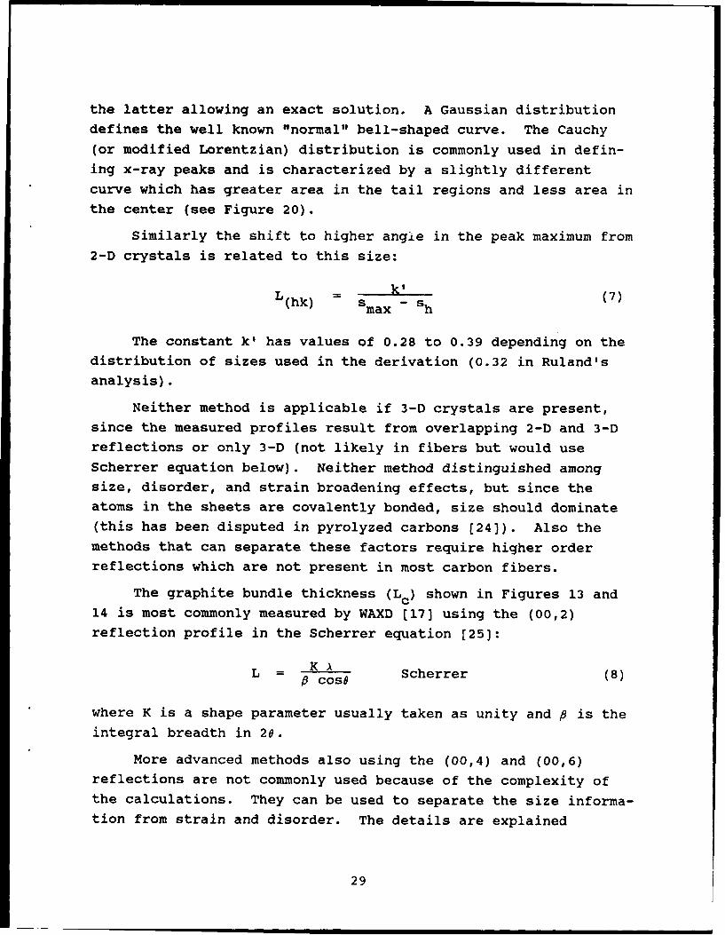
Similarly the shift to higher angle in the peak maximum from2-D crystals is related to this size:

L(hk) - ma S (7)

The constant k' has values of 0.28 to 0.39 depending on thedistribution of sizes used in the derivation (0.32 in Ruland'sanalysis).

Neither method is applicable if 3-D crystals are present,since the measured profiles result from overlapping 2-D and 3-Dreflections or only 3-D (not likely in fibers but would useScherrer equation below). Neither method distinguished amongsize, disorder, and strain broadening effects, but since theatoms in the sheets are covalently bonded, size should dominate(this has been disputed in pyrolyzed carbons [24)). Also themethods that can separate these factors require higher orderreflections which are not present in most carbon fibers.

The graphite bundle thickness (L c) shown in Figures 13 and

14 is most commonly measured by WAXD [17] using the (00,2)reflection profile in the Scherrer equation [25):

L = KALos AScherrer (8)

where K is a shape parameter usually taken as unity and fi is the

integral breadth in 20.

More advanced methods also using the (00,4) and (00,6)

reflections are not commonly used because of the complexity ofthe calculations. They can be used to separate the size informa-tion from strain and disorder. The details are explained

29

0

z0 U

U,

ar

0x.

- C

0E0

NC

0 8

rc) C5d

AiISN3.LNI

30

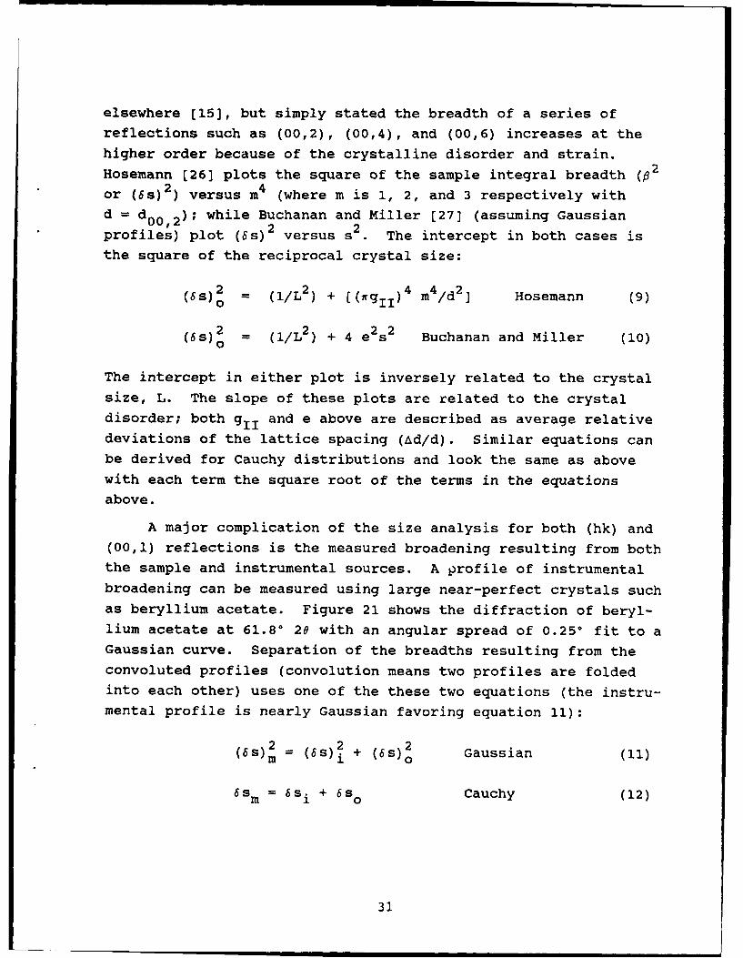
elsewhere (15], but simply stated the breadth of a series ofreflections such as (00,2), (00,4), and (00,6) increases at thehigher order because of the crystalline disorder and strain.Hosemann (26] plots the square of the sample integral breadth (02

or (5s)2 ) versus m4 (where m is 1, 2, and 3 respectively withd = d00 ,2); while Buchanan and Miller (27] (assuming Gaussian

profiles) plot (6s) 2 versus s2 . The intercept in both cases isthe square of the reciprocal crystal size:

(6)2 (/L 2 ) + ((igiI) 4 m4/d 2 ] Hosemann (9)0

(6s) 2 (1/L 2 ) + 4 e2s 2 Buchanan and Miller (10)

The intercept in either plot is inversely related to the crystalsize, L. The slope of these plots are related to the crystaldisorder; both gII and e above are described as average relative

deviations of the lattice spacing (Ad/d). Similar equations canbe derived for Cauchy distributions and look the same as abovewith each term the square root of the terms in the equationsabove.

A major complication of the size analysis for both (hk) and(00,1) reflections is the measured broadening resulting from boththe sample and instrumental sources. A profile of instrumentalbroadening can be measured using large near-perfect crystals suchas beryllium acetate. Figure 21 shows the diffraction of beryl-lium acetate at 61.80 20 with an angular spread of 0.250 fit to aGaussian curve. Separation of the breadths resulting from theconvoluted profiles (convolution means two profiles are foldedinto each other) uses one of the these two equations (the instru-mental profile is nearly Gaussian favoring equation 11):

2 (6s) + (6s)2 Gaussian (11)

6sm = 6s i + 6s0 Cauchy (12)

31

2ra

4 ( 0

4-

0

4

4-

H 414 0

44444-

44

-4 aD>

(\J4

P4J

>44

U H

F- (N

4

es, L es 9 s, WCha(sdoj AIISN31NI

32

An example of the convolution effect of the instrumentalbroadening on a theoretical (00,2) reflection of Lc = 100A is

shown in Figure 22 along with the original curve. With largergraphite crystals with narrower profiles, this effect is morepronounced. A theoretical asymmetric 2-D profile constructedfrom equations 4 and 5 is shown in Figure 23 as well as thisretlection convoluLed with the instrumental profile. Note thatconvolution of the theoretical peak with the instrumental breadth

not only increases the profile width but shifts the peak maximum

to a higher angle as well.

3.4 MISORIENTATION

The structural models shown in section 3.1 show varyingamounts of misorientation of the graphite crystals relative tothe fiber axis. Guigon et al. [11-13) have recently shown that

there are two forms of misalignment: the broad meandering offibrils as shown in Figures 13 and 14, as well as crystals withinfibrils misaligned in so-called "wrinkled sheets." WAXD onlysees the average misalignment including the internal structures

and any misalignment of the fibers in the sample bundle.

Figure 24 shows two typical fiber bundles mounted for WAXD;both show very little if any misalignment of the fibers in theirbundles. This source of error can be considered negligible.

The primary effect of crystal misalignment in WAXD is tobroaden the azimuthal dependence of the intensity. For perfectlyaligned crystals, intensity should be confined to a pair of spotsin a WAXD photo; as the crystals become more misaligned, thespots will grow into arcs which will eventually become rings forcompletely random arrangements of crystals. This broadening ofarcs can be seen in the WAXD photos in Appendix A by examining

the P-series whose arcs become narrower as the fiber modulus

increases.

Several methods for quantifying the azimuthal dependencehave been tabulated [5,17,29], but at best they are only usefulfor relative ranking of materials. The absolute values of the

33

0

w

40

-0 04

o il 4-

0 00 .0o 4-)

N -

Nl 04

0 -x :r

lu~l 0

oj o.HUJ4N

- 0

II

uj 0

X r34

0

0

II I II

wII 00

,-z I I U

D ° c0

/0(0

-400

0 co 4.)0

oo

x /

-0 0 0 04

4.)

I 00

I I II I4-4r-4

P 00I

0 a

IOD

U -4

94 -4

).

N 400

(d m

-~~ -00d

AILISN3LN 1

35

cl

- H

'a4IJ

0 -

0-4

W 'U

.. i I-I

0 4-)

r-41

Q)

F74 4

'r(0 0

>1

E-4

36

azimuthal dependence have been used [see e.g. 13,28J to estimatefiber modulus, but these semi-empirical techniques are not asaccurate as direct mechanical measurements of the fibers.

Figure 25 shows two azimuthal distributions for fibers show-ing the greater breadth for the lower modulus fiber. Reduction ofthe intensity distributions to single numbers includes:

Z = B(1/2,O) = full-width at half maximum in . (13)

r/2 I(o) sin 3 do

R0 Oz /2 (14)

f I(o) sino do

7o1/ 1 8

fF(4) 2 do

a10 = /2 (15)

i F(0) d

where 4 is the fiber colatitude (90°-chi when the fiber is paral-

lel to chi = 00), F(o) is the azimuthal intensity normalized to

= 00, and w/18 = 100.

Equations 14 and 15 require significantly more work thanequation 13 but do not give any additional or more useful infor-mation. Equation 13 is the method of choice for misorientation

of the fibers' graphite planes using the (00,2) reflection full-width at half maximum (FW-HM).

Misorientation of the graphitic planes has been shown aboveto generate azimuthal dependence of intensity. For the (00,2)reflection, this is equivalent to the crystal plane normalssweeping out not a plane but a solid figure centered about theequator. One can think of a continuous mountain ridge of con-stant height circling the equator, the height of this ridgeproportional to the probability of a crystal normal existing atthat latitude. A very sharp ridge corresponds to a highly

37

U;

0

*04

0

01 4

F-aM*

CN

U))F-

"*$? MII sosWgwhnw eAIS3N 3~U3

38n

oriented fiber, and a poorly oriented fiber would have a gentlysloping ridge.

The meridional reflections' (hk) and (hk,0) normals orienta-tion probabilities can be viewed as mountains at each of thepoles. The (00,2) full-width at half maximum will also definethe (hk) and (hk,0) misorientation mountain FW-HM (this will beconvoluted into the persistence length probabilities mountain of

section 3.1). Misorientation is the major reason the (10) and/or(10,0) reflection is visible in flat-film photos and why itsintensity decreases as the crystal orientation increases (seeagain the P-series of photos in Appendix A).

Off-axis reflections also become visible from misorientationas explained near the end of section 2.2. The intensity of the

(10,1) reflections in the WAXD photos of higher modulus fibers isgenerally greater than (10) and (10,0) even though the maximumprobability is lower, because at the collection angles relativeto the fiber axis (also called colatitudes) which are equal toone-half the respective Bragg angles, the probabilities are

generally greater.

39

4. RESULTS

4.1 MATERIALS

A series of commercially available carbon fibers were exam-ined in this study. Those fibers, their manufacturers, and someof their published mechanical properties are listed in Table 1.These fibers were picked because of their range of properties andavailability. Both Pitch-based (P-series) and PAN-based fiberswere included for comparison.

In addition, an experimental annealed vapor grown carbonfiber was includedI as an example of a very highly graphitizedfiber. This fiber was supplied courtesy of Dr. Karren K. Britoof Applied Sciences, Inc., Yellow Springs, OH.

4.2 (00,2) RESULTS

The (00,2) results from WAXD for the samples above are given

in Table 2. These results include d 00,2, Lc, and Z00,2 Thed00,2 is from the position of the (00,2) reflection measured bycurve fitting [34] the WAXD Bragg scan at chi=00 (equatorialscan) and using Bragg's Law (equation 2). Figure 26 shows anexample of the curve-fit (00,2) reflection using P-55 with a =

0.8590 and d0 0 2 = 3.523A from a maximum at 25.28 ° 26. In thistable Lc is calculated from the Scherrer equation (equation 8)using the same curve fit as d00,2 corrected for instrumentalbroadening by equation 11. An azimuthal scan of (00,2) reflec-tion was curve fit to obtain the full-width at half maximum orZ00,2 of each fiber. Figure 27 shows P-55's azimuthal scan forthe (00,2) reflection (Z0 0 ,2 = 14.10).

The trends seen here have been observed beforet d00,2 andZ00,2 decrease, while Lc increases as the measured tensile modu-

lus increases. Apparently the big changes occur as the modulus0 0

passes 50 Msi: Lc increases from 20-30A to greater than 100A,and Z00 ,2 drops rapidly to single digits.

The differences between Pitch- and PAN-based fibers can beseen by comparing equivalent (modulus) pairs of fibers; e.g. P-25

40

TABLE 1

FIBER MECHANICAL PROPERTIES [30-33]

Tensile Tensile CompressiveModulus Strength Strength

Fiber Manufacturer Msi (GPa) ksi (GPa ksi (GPa)

P-25 AMOCO 23 (159) 200 (1.38) 167 (1.15)

P-55 " 55 (379) 250 (1.72) 123 (0.85)

P-75 75 (517) 300 (2.07) 100 (0.69)

P-100 105 (724) 325 (2.24) 70 (0.48)

P-120 120 (827) 325 (2.24) 65 (0.45)

T-300 AMOCO 34 (231) 470 (3.24) 417 (2.88)

AS4 Hercules/Magnamite 34 (231) 528 (3.64) 390 (2.69)

T-40 AMOCO 42 (290) 500 (3.45) 400 (2.76)

G40-700 BASF/Celion 44 (300) 720 (4.96) na

IM6 Hercules/Magnamite 45 (308) 620 (4.27) na

G45-700 BASF/Celion 45 (310) 700 (4.83) na

HMS Hercules/Magnamite 50 (345) 320 (2.21) na

T-50 AMOCO 57 (393) 350 (2.41) 233 (1.61)

GY-70 BASF/Celion 75 (517) 270 (1.86) 153 (1.05)

na - Not available

41

I I I I I I

TABLE 2

SUMMARY OF (00,2) WAXD CARBON FIBER RESULTS

do0,2 L0c Z0,2Fiber (Angstroms) (Anastroms) (degrees FW-HM)

Pitch-Based

P-25 3.479 26 31.9

P-55 3.426 114 14.1

P-75 3.416 157 11.0

P-100 3.385 208 5.6

P-120 3.378 228 5.6

PAN-Based

T-300 3.496 16 35.1

AS4 3.521 10 36.8

T-40 3.515 17 30.2

G40-700 3.495 21 29.1

IM6 3.464 20 33.7

G45-700 3.470 25 26.7

HMS 3.427 62 19.7

T-50 3.429 57 16.4

GY-70 3.405 173 9.6

Vapor Grown

AppliedSciences 3.373 345 14.8

42

* U;

0

0

4.,

1-1)3 (4

04

Q)

* $4

U

'0

('4

'Dn

(5d) AIISN3iNI

43

U1

44

I. 4-4

00

CN

$-

mmU.

I n I

(SdD) AI:SN3INI

44

and AS4, P-55 and T-50, and P-75 and GY-70. The first and thirdpairs' properties are roughly equivalent. In the second pairP-55 appears to have made the morphological jump to larger, moreperfect crystals and T-50 is intermediate between the higher and

lower modulus morphology indicating some lag in the developmentof larger structures in PAN-based fibers as the modulus isbuilt-up in processing.

The vapor grown Applied Sciences carbon fiber does not haveas highly oriented planes (Z0 0 ,2 = 14.80) but the graphitization

is much higher than the other fibers since the d = 3.373A is000,2 athe closest to the ideal 3.3535A and the crystal size, Lc = 345A,

is the largest measured.

4.3 ADVANCED Lc RESULTS

The advanced L techniques of Hosemann or Buchanan andcMiller require higher order reflections. Figure 28 shows a com-

plete equatorial scan of P-100 with the higher order (00,1)reflections. only 8 of the 15 fibers examined had all three(00,1) reflections resolvable for use in determining which of thetechniques to use (the remaining 7 fibers did have two orders).

The two techniques for separating crystalline disorder from

size broadening of Hosemann and Buchanan and Miller eachexpressed for both Gaussian (equations 9 and 10) or Cauchy dis-tributions yield four possible plots. Figures 29-32 show these

four plots for P-55. Table 3 gives each plot's correlation coef-

ficient and root mean square error (averages for the 8 fibers

used here).

While the correlation coefficient for both of the Buchananand Miller plots is only slightly smaller than the Hosemann plotsand the Gaussian line actually gives the lowest RMS, this methodwas not considered correct since as often as not the interccptvalues were negative. This would give a physically impossible

negative crystallite size.

45

'-44

0

U)

On)

0 0

46-

00

04-4

0

4

U)

0

0 it

tn E

EALA.

I4P

In 0 0

0

J0

10 10 10 1 ) 0 0 C

x x x x x

cn

47

04-4

0-1-

.4J

U)--4

>1

4-

U

Nu

LA

0 04-4 M)

0r-4 Q

--4

N ~ r-4

05-I

0

0 Q)N 0

0 U)--4

o d00

48

ODU

0 U)

1

* 'U

*134

uL O

40 r.

0 (d

4 Eno o

>1

?10~44d 4-)

, -.4 ,.

100 0 0

IC)~~r 4 4.)- ~u )i

-0-

44

No

do

49

.)6 C

wF<1 I1(0

a-4Lo

, -4

U) 044 -,4

.,-I

4J -

0)0a4 0)

r-4

50

. I

0N10

0 0

0U)40

50

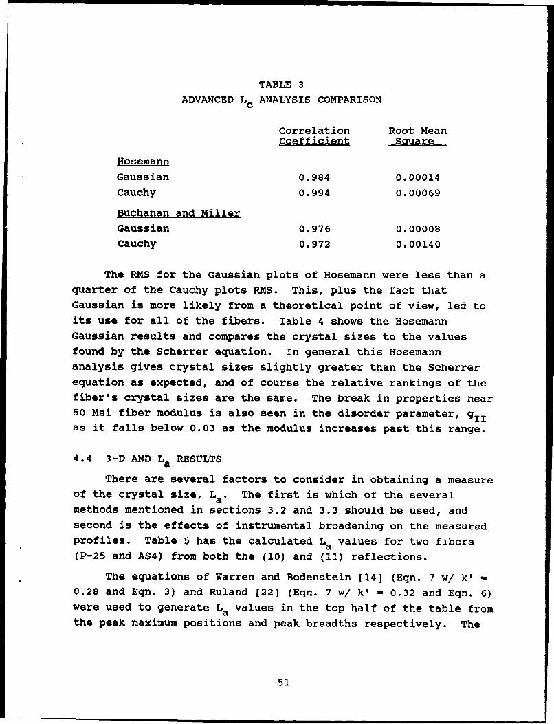
TABLE 3

ADVANCED Lc ANALYSIS COMPARISON

Correlation Root Mean

Coefficient Sauare

Hosemann

Gaussian 0.984 0.00014Cauchy 0.994 0.00069

Buchanan and MillerGaussian 0.976 0.00008

Cauchy 0.972 0.00140

The RMS for the Gaussian plots of Hosemann were less than aquarter of the Cauchy plots RMS. This, plus the fact thatGaussian is more likely from a theoretical point of view, led to

its use for all of the fibers. Table 4 shows the HosemannGaussian results and compares the crystal sizes to the values

found by the Scherrer equation. In general this Hosemannanalysis gives crystal sizes slightly greater than the Scherrerequation as expected, and of course the relative rankings of the

fiber's crystal sizes are the same. The break in properties near50 Msi fiber modulus is also seen in the disorder parameter, gIIas it falls below 0.03 as the modulus increases past this range.

4.4 3-D AND La RESULTS

There are several factors to consider in obtaining a measureof the crystal size, L a . The first is which of the several

methods mentioned in sections 3.2 and 3.3 should be used, andsecond is the effects of instrumental broadening on the measuredprofiles. Table 5 has the calculated La values for two fibers(P-25 and AS4) from both the (10) and (11) reflections.

The equations of Warren and Bodenstein [14] (Eqn. 7 w/ k'0.28 and Eqn. 3) and Ruland [22] (Eqn. 7 w/ k' = 0.32 and Eqn. 6)were used to generate La values in the top half of the table fromthe peak maximum positions and peak breadths respectively. The

51

TABLE 4

ADVANCED Lc ANALYSIS RESULTS

Number of Lc (Angstroms) Disorder

Fiber Orders Used Hosemann Scherrer (gii)

Pitch-Based

P-25 2 36 26 0.0794

P-55 3 99 114 0.0301

P-75 3 140 157 0.0233

P-100 3 159 208 0.0166

P-120 3 188 228 0.0182

PAN-Based

T-300 2 19 16 0.0820

AS4 3 15 10 0.0694

T-40 2 21 17 0.0688

G40-700 2 27 21 0.0707

IM6 2 24 20 0.0785

G45-700 2 29 25 0.0626

HMS 3 78 62 0.0413

T-50 3 66 57 0.0409

GY-70 3 138 173 0.0305

Vapor Grown

AppliedSciences 3 374 345 0.00828

52

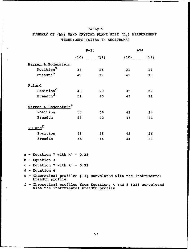
TABLE 5

SUMMARY OF (hk) WAXD CRYSTAL PLANE SIZE (La) MEASUREMENT

TECHNIQUES (SIZES IN ANGSTROMS)

P-25 AS4

(10) (11) (10) (11)

Warren & Bodenstein

Positiona 35 26 31 19

Breadthb 49 39 41 30

Ruland

Positionc 40 29 35 22

Breadthd 51 40 43 31

Warren & Bodenstein e

Position 50 36 42 24

Breadth 53 42 43 31

Rulandf

Position 48 38 42 26

Breadth 55 44 44 33

a - Equation 7 with k' = 0.28

b - Equation 3

c - Equation 7 with k' = 0.32

d - Equation 6

e - Theoretical profiles [14] convoluted with the instrumentalbreadth profile

f - Theoretical profiles from Equations 4 and 5 [22] convolutedwith the instrumental breadth profile

53

bottom half of the table went back to the original equations

(such as equations 4 and 5) for these workers, generated a series

of profiles for varying crystal sizes, and then folded the

instrumental profiles into those theoretical curves. These con-

voluted profiles were then compared to the experimental curves to

again get measures of La from the peak maximum positions and

breadths.

As pictured in Figure 23, the instrumental broadening

affects the measured profiles; but at the crystal sizes of these

fibers, the differences are not as great as the differences be-

tween the position and breadth calculations. The variation

between the two groups is even less. Considering the work in-

volved in the correction for the instrumental broadening and the

lack of better results when it is used (except to make the posi-

tion and breadth results closer), it should be dropped. A good

compromise in effort and results is to use Equation 6 to calcu-

late La values.

The reason P-25 and AS4 were chosen for Table 5 is that both

show no evidence of 3-dimensional crystals. The presence of 3-D

crystals is another problem associated with calculating La since

the equations used above all assume simple 2-D crystals and are

not valid for 3-D or mixtures of 2-D and 3-D crystal reflections.

Once the presence of 3-D crystals is detected, one can assume

that mixed reflections are confounding the measurements.

Three-dimensional crystals are not easy to detect in merid-

ional scans. As mentioned in section 2.3, off-axis reflections

can be seen in meridional scans only when crystal misorientation

is larger than the crystal tilt from the fiber axis; as will be

seen below, 3-D crystals occur in fibers with low misorientation.

Tilting fibers to chi<900 or by the omega circle is necessary to

reveal emerging 3-D reflections. This can be seen in Figure 33

which is a multiple plot of P-100 fiber diffraction obtained at

chi=900 , chi=70 ° (at omega=0 °) and chi=90 ° (at omega=200 ). The

chi=90 ° or meridional scan shows absolutely no sign of the

(10,I), but the other two scans are dominated by that reflection.

54

U)

0

'-4

V~ p~

T4Uk '4-

0 -

44-

44 0E~

r-4 4

10

-- 44

AIISNI.N! JAl1U138

55

Figure 34 is a complete meridional scan of P-100, and Figure 35is a complete scan taken at chi=70 ° . Both scans have the majorreflections annotated.

The two major off-axis reflections (10,1) and (11,2) aretilted 17.60 and 20.20 from the fiber axis so that chi=700 (90 ° -

200) (or omega=200 ) is close enough to the crystal tilt angle toobserve either reflection. The error in (10,I) of 2.40 is lessthan any of these fibers misorientation and errs at an angle onthe far side of the (10,0) reflection which is the major sourceof interference. Ideally each reflection should be examined atits optimum tilt angle, but practical considerations limited thecurrent data collection.

The ideal locations [18] of the (10,0) and (10,1) reflec-tions are 42.40 and 44.60 respectively. Since each these peakshave typical full-widths at half-maximum of a few degrees, finitecrystal sizes push the 2-D reflections to higher angles, andcrystalline disorder of 3-D crystals push their reflections tolower angles, these reflections will almost always overlap. Thisoverlap is shown in Figure 33 for P-100 which is generallyaccepted as having significant 3-D crystalline character. Onlyin the Applied Sciences' vapor grown carbon fiber are the (10,0)and (10,1) reflections resolved (see Appendix B).

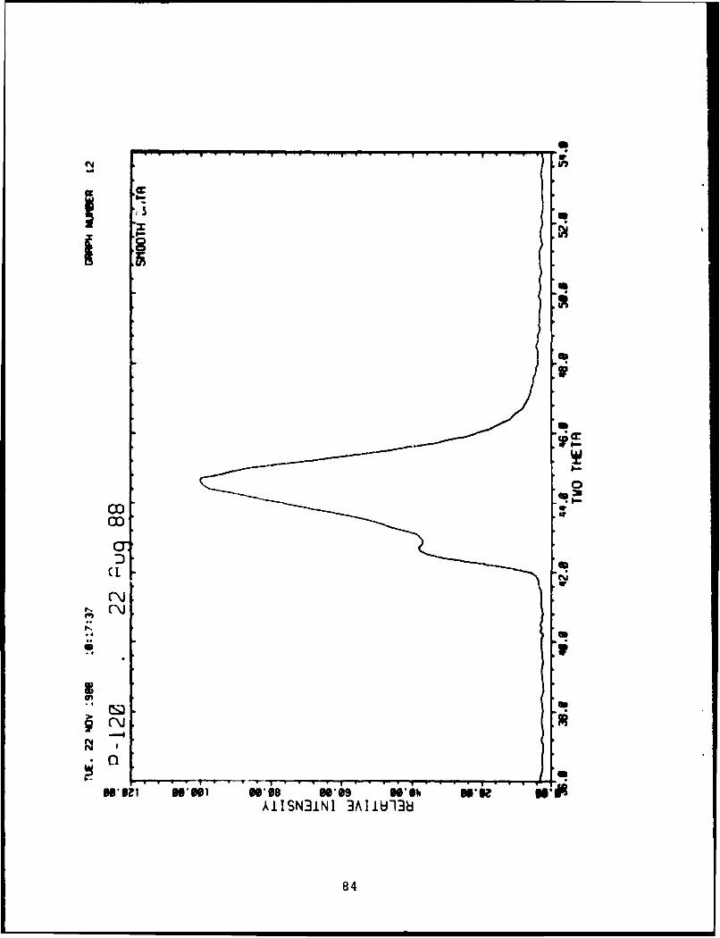
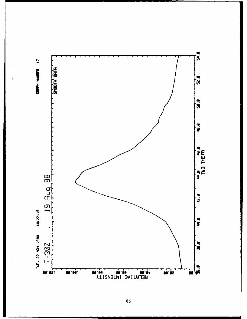
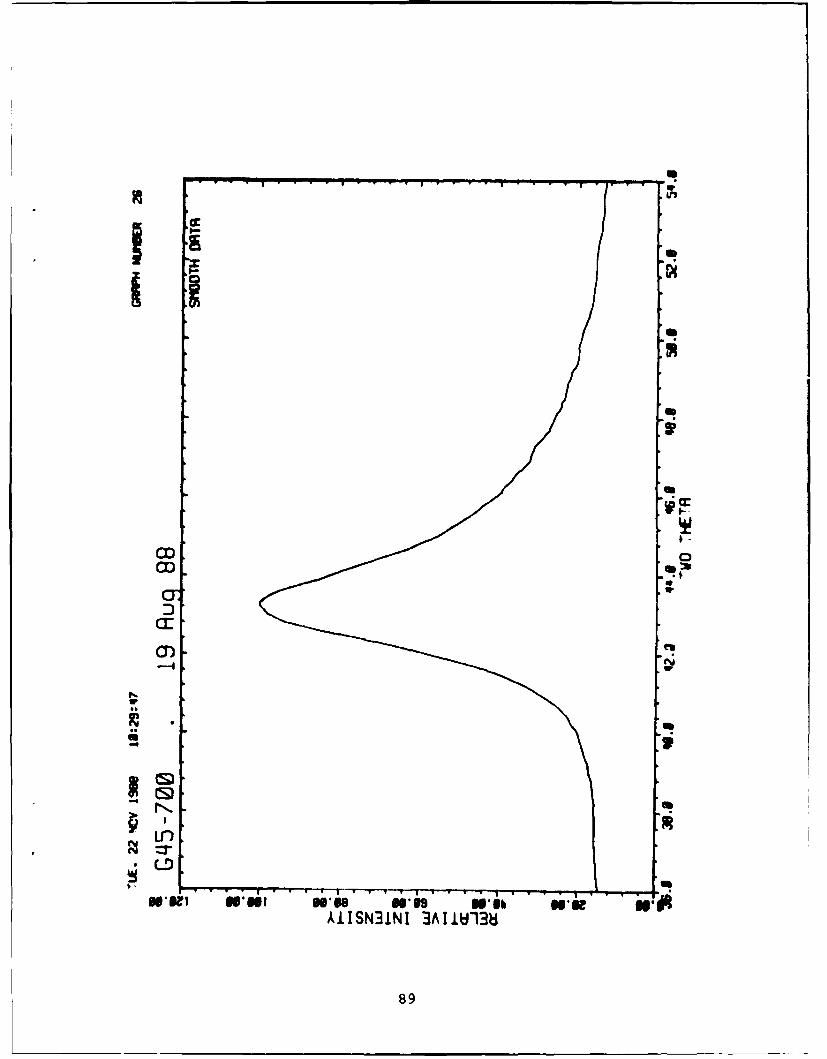
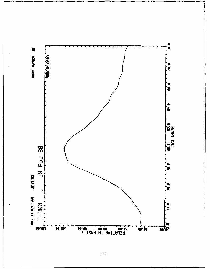
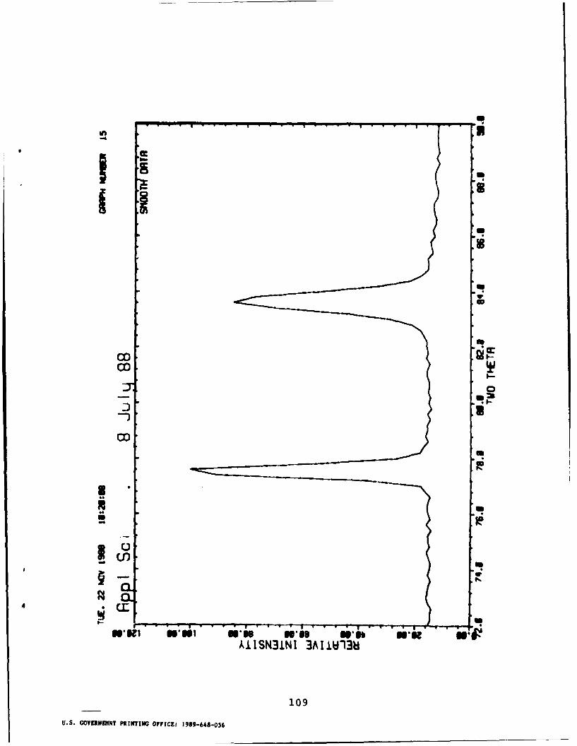
The (11,2) off-axis reflection is more useful than the(10,1) to look for since it can be resolved better as the ideallocations [18] of the (11,0) and (11,2) reflections are 77.50 and83.50 (see Appendix C). This is particularly obvious in transi-tion fibers such as P-75 and GY-70; their (10,1) regions showwhat appears to be overlapping peaks, but their (11,2) regionsshow definite emergence of the off-axis reflection. Individualscans are in Appendices B and C, while multiple plots of severalPitch-based fibers are shown in Figures 36 (10,1) and 37 (11,2)and in Figures 38 (10,1) and 39 (11,2) for PAN-based fibers.

In the (10,I) region multiple plots, the overlap between(10,0) and (10,1) apparent in P-75 and GY-70 is also possible for

56

ea 0

0

C)

0o m

I.))

0000

0r

(S :

-4)

9S0Z o il 000 '0,9 00-6h o4a

57

N Cu

Iall0

0

(15

-4 '4444I0

ul 1

2r L)

a

'A- -, L4

C0

AIISN31NI 3A11U138

58

0

IC)IlW)IC

.1 0

00

*1 0

4-4000

0060

0Sfn

C) \.

Ux

'0co) w fq

AISN1N 3A.'3

Z 59

00

/I 9

Mm

ODII. 44

C?)

OD0 0

0~1 0II z o~

00

0D W1 0x.. . i

U,)

ODO

00

0 00I 0\00 0

0 ~60

* IC)I. 0

0 r%4I0t0

0 ID'0

0

1000looo

100,Ole 0

0000

44

0

0 0 00 00t

~0 0 D I

610

00

0 1o I."o,

I

J Z,/4

10104

0

I.. 0./ 0 0

0

OD 0

62CJ

,I I

000

00

0 000 00 D W ~

AISNN 3Al~l

4 62

the next lower modulus pairs of P-55 and T-50. Claiming partial3-D crystals from this data alone is definitely unwarranted. Thefact that each series peak maxima coincide precisely for P-55 and

P-75, and T-50 and GY-70 but not with the lower modulus fiber,supports the claim of some 3-D crystals. Returning to Table 5,note that the (10) reflection yields larger La values than the(11) reflection for both of those fibers. This is true for otherfibers as well, as seen in Table 6 (La values calculated using

equation 6) except in the cases of known or surmised 3-D crys-

tals.

Three-dimensional crystals have been reported for both Pitch

and PAN-based carbon fibers [34) but only at moduli at or greaterthan 100 Msi. The observation of 3-D crystals at lower moduli inthis study is a direct result of the use of the tilted fiber

technique.

Table 6 should have been the last word on La values here butfor the 3-D crystal problem and the truncation in 20 of the (hk)

patterns as shown in Figure 19. This truncation reduces thebreadth of the diffraction peak resulting in a higher value Laalthough the complete lack of (hk,l) interference is helpful.

These crystals should be larger as measured at the chi=90 ° com-pared to chi=70 ° leading to the conclusion that the last two

columns in Table 6 should be considered as maximum limiting

values.

If one assumes that when the value of La at chi=700 from(10) falls near or below the value from (11) this is an indica-tion of 3-D crystals developing (two paragraphs above), then the

suspected samkles with 3-D crystals in the last paragraph are

confirmed. This point also coincides with a large deviation inmeasured La between chi=90 ° and chi=70 ° , but that may be fortui-tous. Table 7 lists the fibers and whether they contain 2-D

crystals only, some 3-D crystals, or suspected 3-D crystals.

63

TABLE 6

SUMMARY OF (hk) WAXD CRYSTAL PLANE SIZES (La IN ANGSTROMS)

Chi = 70* Chi = 900

Fiber (10) (11) (10) (11)

Pitch-Based

P-25 51 40 49 43

P-55 83 ill 236 201

P-75 64 172 265 276

P-100 naa 306 328 372

P-120 naa 327 379 395

PAN-Based

T-300 43 37 46 36

AS4 43 31 47 39

T-40 44 34 54 38

G40-700 64 49 75 62

IM6 nab nab 58 52

G45-700 61 45 77 61

HMS 143 96 181 171

T-50 91 88 177 165

GY-70 62 153 265 293

Vapor Grown

AppliedSciences 338 394 333 395

na - Not availablea - (10,1) obviously dominating the scan areab - Bragg scan not obtained

64

TABLE 7

SUMMARY OF CARBON FIBER 2-D AND 3-D CRYSTAL CONTENT

2-D Crystals 3-D Crystals

Fiber Only Suspected Definite

P-25 x

P-55 - x

P-75 - - x

P-100 - - x

P-120 - - x

DuPont - - x

T-300 X - -

AS4 X - -

T-40 X - -

G40-700 X - -

IM6 X - -

G45-700 X - -

HMS X- -

T-50 X -

GY-70 X

Vapor Grown

AppliedSciences X

65

4.5 OTHER

In Figure 5 the diffraction of P-100 (and P-120 from

Appendix A) shows satellite intensity of the (10,1) reflection at

the 600 positions relative to the main intensity at chi=900 . The

source of these peaks is obviously from flattened graphitic bun-

dles with sufficiently large flat regions to allow diffraction

from the equivalent (hk,l) crystal planes of the reflection gen-

erating the main peak. Preferred orientation of the large

bundles is also necessary, since with random orientation of the

a-axis and flattening of the bundles, a ring should develop as

those equivalent crystal planes would also be random (see section

3.1). Because satellite peaks have developed only at specific

locations around the ring area, only those sheet bundles properly

oriented can flatten out during the general crystal orientation

and perfecting processing.

Additional data, including (11,2) orientation, is required

to properly interpret these hints of structure in highly

oriented, high modulus carbon fibers.

66

5. CONCLUSIONS

The general crystalline structure of Pitch- and PAN-basedcarbon fibers is roughly equivalent for fibers of approximately

the same tensile modulus. The major structural changes occur infibers of 50-60 Msi modulus, with the PAN-based fibers laggingbehind the Pitch-based fibers only slightly in terms of structureversus modulus development. Some of the major differences

between these two classes of fibers is due more to the difficultyof processing to achieve PAN-based fibers with sufficiently highmodulus to compare with common Pitch-based fibers than any inher-ent structural differences.

The large strength differences in these classes of fibersare apparently not directly related to the crystal sizes andaverage orientation of those crystals. Internal crystal arrange-ment and gross flaws, which are not detectable in WAXD measure-ments on neat fibers, may be responsible for the strength

characteristics.

67

REFERENCES

1. A. Fourdeux, C. Herinckx, R. Perret, and W. Ruland,Translated Title: "Physical Chemistry - The Structure ofCarbon Fiber," C. R. Acad. Sci., 269, 1597 (1969).

2. R. Perret and W. Ruland, "The Microstructure of PAN-BaseCarbon Fibres," J. Appl. Cryst., 3, 525 (1970).

3. A. Fourdeux, R. Perret, and W. Ruland, Proc. First Int.Conf. on Carbon Fibers, London, Plastics Inst. (1971).

4. J. V. Larsen and T. G. Smith, "Carbon Fiber Structure,"NOLTR 71-166, Naval Ordnance Laboratory, White Oak, SilverSpring, MD, October 1971.

5. R. Bacon, "Carbon Fibers from Rayon Precursors," inChemistry and Physics of Carbon: A Series of Advances, Vol.9 (1973), P. L. Walker Jr. and Peter A. Thrower, Eds.,Marcel Dekker, Inc., New York.

6. F. R. Barnet and M. K. Noor, Proc. Second Int. Conf. onCarbon Fibers, London, Plastics Inst. (1974).

7. F. R. Barnet and M. K. Noor, "A Three-Dimensional StructuralModel for a High Modulus PAN-Based Carbon Fiber," NOLTR73-154, Naval Ordnance Laboratory, White Oak, Silver Spring,MD, June 1974.

8. R. J. Diefendorf and E. W. Tokarsky, "High-PerformanceCarbon Fibers," Polymer Eng. Sci., 15, 150 (1975).

9. S. C. Bennett, D. J. Johnson, and R. Murray, "StructuralCharacterization of a High-Modulus Carbon Fibre by High-Resolution Electron Microscopy and Electron Diffraction,"Carbon, 14, 117 (1976).

10. S. C. Bennett and D. J. Johnson, "Electron-MicroscopeStudies of Structural Heterogeneity in PAN-Based CarbonFibers," Carbon, 17, 25 (1979).

11. M. Guigon, A. Oberlin, and G. Desarmot, "Microtexture andStructure of Some High Tensile Strength, PAN-Base CarbonFibres," Fibre Sci. Technol., 20, 55 (1984).

12. M. Guigon, A. Oberlin, and G. Desarmot, "Microtexture andStructure of Some High-Modulus, PAN-Base Carbon Fibres,"Fibre Sci. Technol., 20, 177 (1984).

13. M. Guigon and A. Oberlin, "Heat-Treatment of High TensileStrength PAN-Based Carbon Fibres: Microtexture, Structureand Mechanical Properties," Compos. Sci. Technol., 27, 1(1986).

68

itI I I l I I II

14. B. E. Warren and P. Bodenstein, "The Shape of Two-Dimensional Carbon Black Reflections," Acta Cryst., ?Q, 602(1966).

15. L. E. Alexander, X-Ray Diffraction Methods in PolymerScience, Wiley-Interscience, New York, 1969.

16. A. Fourdeux, R. Perret, and W. Ruland, "The Effect ofPreferred Orientation on (hk) Interferences as Shown byElectron Diffraction of Carbon Fibres," J. App1. Cryst.,1, 252 (1968).

17. W. Ruland, "X-Ray Diffraction Studies on Carbon andGraphite," in Chemistry and Physics of Carbon: A Seriesof Advances, Vol. 4 (1968), Philip L. Walker Jr., Ed.,Marcel Dekker, Inc., New York.

18. Joint Committee on Powder Diffraction Standards, "Graphite,"

JCPDS 23-64 (1973).

19. M. von Laue, Z. Kristallogr., 82, 127 (1932).

20. B. E. Warren, Phys, Rev., 59, 693 (1941).

21. A. J. C. Wilson, "X-Ray Diffraction by Random Layers: IdealLine Profiles and Determination of Structure Amplitudes fromObserved Line Profiles," Acta Cryst., 2, 245 (1949).

22. W. Ruland, "Fourier Transform Methods for Random-Layer LineProfiles," Acta Cryst., 22, 615 (1967).

23. W. Ruland and H. Tompa, "The Effect of Preferred Orientationon the Intensity Distribution of (hk) Interferences,"Acta Cryst., A24, 93 (1968).

24. W. Braun and E. Fitzer, "A Modified Structural ModelDescribing the Interference-Function of Pyrolized Non-Graphitizing Carbon," Carbon, 16, 81, (1978).

25. P. Scherrer, Gottinger Nachrichten, 2, 98 (1918).

26. R. Bonart, R. Hosemann, and R. L. McCullough, Polymer,4, 1 (1963).

27. D. R. Buchanan, R. I. McCullough and R. L. Miller,"Crystallite Size and Lattice Distortion Parameters fromX-ray Line Broadening," Acta Cryst., 20, 922 (1966).

28. W. N. Reynolds and J. V. Sharp, "Crystal Shear Limit toCarbon Fibre Strength," Carbon, 12, 103 (1974).

29. J.-B. Donet and R. C. Bansal, Carbon Fibers, MarcelDekker, Inc., New York, 1984, Chapter 2.

69

30. S. Kumar, W. W. Adams, and T. E. Helminiak, "UniaxialCompressive Strength of High Modulus Fibers for Composites,"J. Rein. Plast. Compos., 2, 108 (1988).

31. S. Kumar, "Structure and Properties of High PerformancePolymeric and Carbon Fibers - An Overview," Fiber Prod.Conf. Proc. (1988).

32. K. Strong, personal communications.

33. J. D. H. Hughes, "The Evaluation of Current Carbon Fibres,"Phys. D: Appl. Phys., 20, 276 (1987).

34. M. S. Dresselhaus, G. Dresselhaus, K. Sugihara, I. L. Spain,and H. A. Goldberg, Graphite Fibers and Filaments, Springer-Verlag, New York, 1988, Chapt. 3.

70

APPENDIX A

FLAT-FILM WAXD PHOTOGRAPHS OF CARBON FIBERS

Pitch PAN

P-25 T-300 G45-700

P-55 AS4 HMS

P-75 T-40 T-50

P-100 G40-700 GY-70

P-120 1M6

71

Ln

LA)

72

4

P.4

7 3

E-4

74

75

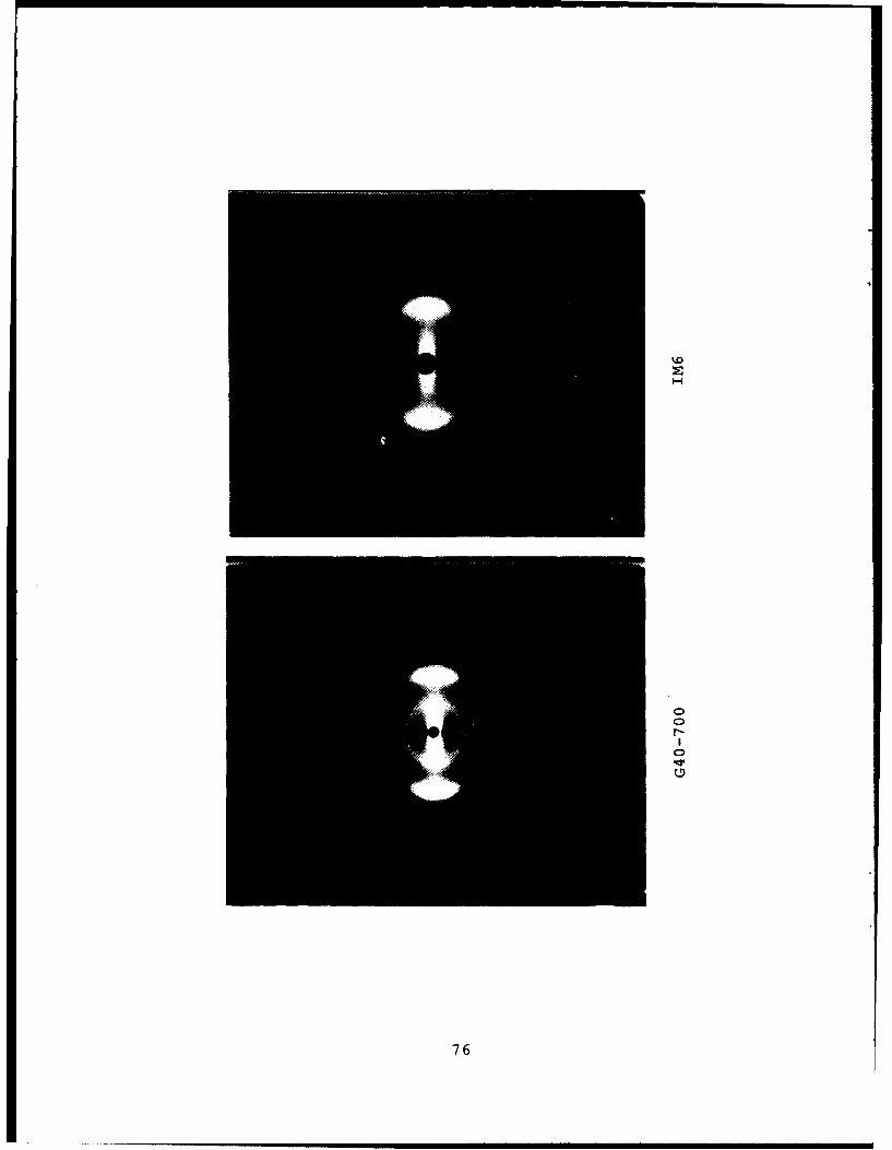
I~o

H

00

0

0

76

00

LA

0

77

E-4

78

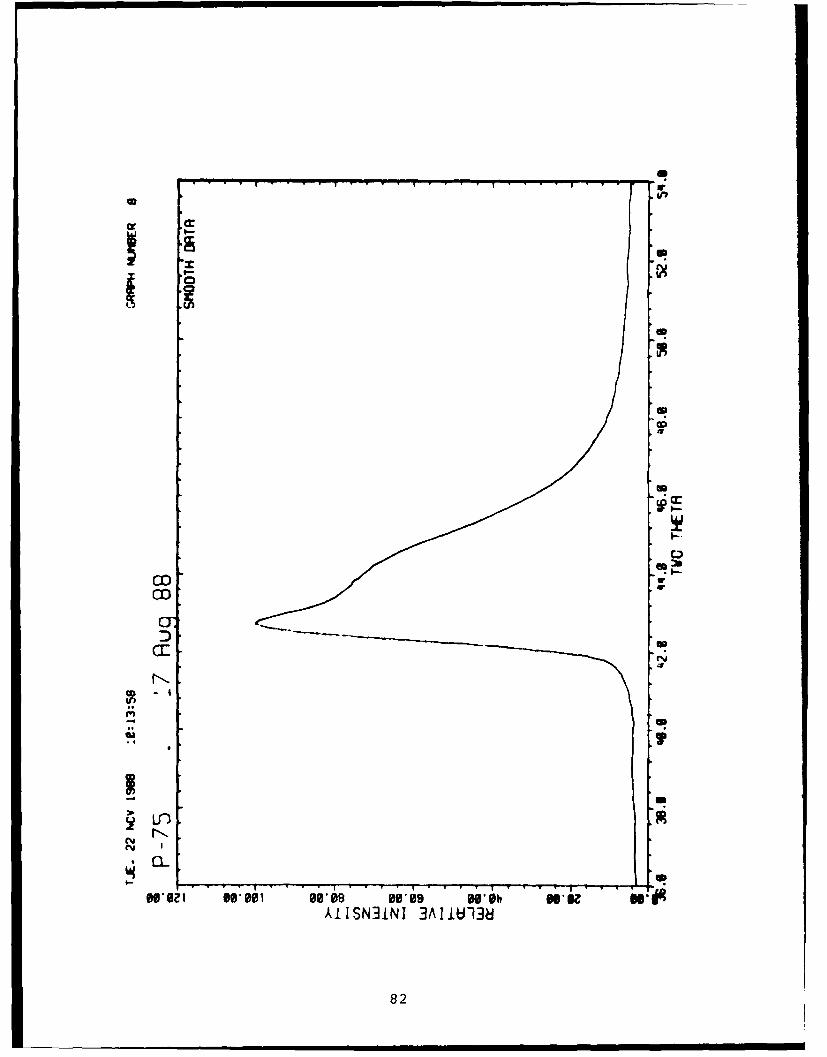
APPENDIX B

DIFFRACTION SCANS (CHI=70° ) OF THE (10) AND (10,1) REGIONOF THE CARBON FIBERS

Pitch PAN Vapor Grown

P-25 T-300 G45-700 Applied Sciences

P-55 AS4 HMS

P-75 T-40 T-50

P-100 G40-700 GY-70

P-120

79

Ir- IorPII

cn

WWI "1 0,6 09AiS3N 3AlU3

80I

mU

CC,

Uor

IOLnU

MIMI Wool99,9 "Is UlAiISN1NI 3UU13

81a

CDU

cc.

OD

U-3

CL,

AIISNiNI 3.lUI3

G82

CC 'U I5 ' I

IIar

040

04 t

IN -ei Igo-g 00,9 "lb WU

AIIS31N 3Al 3

83,

gS

. ...... ........ ..I0coS

000

CL

gU.

.484

U

IO.-

IiIsco

000

cnD

a I

AIISN3I 3AI1U13b

85

CL I

ry U)

cn90*9 90*9 al% a

AIS3Nn3~U3

86U

l-

Worin W"s WIN go" ~ b UluAIISN31NI 3AIlUI38

87

coSco

a)I~

rN. -

LDS

V ---- T V

991W W"IN~s MIRwit

AISN1N 3A03

w8

CC

ICDU

LDU

AIISNNI 3AlUI3

89U

x.

I Um

1cr

.1-

cocxo

0

0090

Ir-.

911

Ur

0a)-co

I- r-

cnS3N 3~U3

J 92

Iria InCLU

CCU

AIISN1NI 3IIU13

93U

APPENDIX C

DIFFRACTION SCANS (CHI=70') OF THE (11) AND (11,2) REGION

OF THE CARBON FIBERS

Pitch -PNVapor Grown

P-25 T-300 G45-700 Applied Sciences

P-55 AS4 HMS4

P-75 T-40 T-50

P-100 G40-700 GY-70

P-120

95

M,

Lj

AISN1N 3A33

96U

co

co

coI I

a-1

. . .W eil. .

AIISNNI 3UU13

97.

U-)

CL3

WIWI WIWI 00*8 W19 a-t i

AIISN1N] 31103

98U

a)a

I.-

u~g~1 w~u1 ~ sB o

c99

ccI

N

AISNN 3A3U3100

-4r

Di -

AISN1N 3AIU

101

-3

le

cv

ci:

U 'U ~ iWC ~ i-b . 'j. .WJ

102

0,103

a)

.10

IO

0,0

a) mw

-4w MII "l.-9 eb MRU

AllS~~l 3UU13

10

OU

3LfO4

0c

co30a)

in

N*Z0061 0,8 00-09 0$ib OWN a-IVAIISN31NI 3AIlUI38

106

II

U')

WN3

AIISN1NI 3~lUI3

.1107

ii U:

co 3coU

cr3

DS

Loe

W. a MII WI W-m, N'T .. i. i in 0m

A.LISKNI 3~lUI3

108

in

-CD

a

:7.

D-.Cm

AI1SN3i1 3A^ 173H1

109

US. COVZRNIgNT PRINTING OFFICE: 1989-648-056