Policy Research Working Paper 8058

Compensation, Diversity and Inclusion at the World Bank Group

Jishnu DasClement Joubert

Sander Florian Tordoir

Development Research GroupHuman Development and Public Services TeamMay 2017

WPS8058P

ublic

Dis

clos

ure

Aut

horiz

edP

ublic

Dis

clos

ure

Aut

horiz

edP

ublic

Dis

clos

ure

Aut

horiz

edP

ublic

Dis

clos

ure

Aut

horiz

ed

Produced by the Research Support Team

Abstract

The Policy Research Working Paper Series disseminates the findings of work in progress to encourage the exchange of ideas about development issues. An objective of the series is to get the findings out quickly, even if the presentations are less than fully polished. The papers carry the names of the authors and should be cited accordingly. The findings, interpretations, and conclusions expressed in this paper are entirely those of the authors. They do not necessarily represent the views of the International Bank for Reconstruction and Development/World Bank and its affiliated organizations, or those of the Executive Directors of the World Bank or the governments they represent.

Policy Research Working Paper 8058

This paper is a product of the Human Development and Public Services Team, Development Research Group. It is part of a larger effort by the World Bank to provide open access to its research and make a contribution to development policy discussions around the world. Policy Research Working Papers are also posted on the Web at http://econ.worldbank.org. The authors may be contacted at jdas1@worldbank.org.

This paper examines salary gaps by gender and nationality at the World Bank Group between 1987 and 2015 using a unique panel of all employees over this period. The paper develops and implements a dynamic simulation approach that models existing gaps as arising from differences in job composition at entry, entry salaries, salary growth and attri-tion. There are three main findings. First, 76 percent of the $27,400 salary gap across the average male and female staff at the World Bank Group can be attributed to composi-tion effects, whereby men entered the World Bank Group at higher paid positions, particularly in the earlier half of the sample. Second, salary gaps 15 years after joining the

World Bank Group can favor either men or women depend-ing on their entry position. Third, for the most common entry-level professional position (known as Grade GF at the World Bank Group) there is a gender gap of 3.5 per-cent in favor of males 15 years after entry. The majority of this gap (84 percent) is due to differences in salary growth rather than differences in entry salaries or attrition. The pattern of these gaps is similar for staff from different nationalities. The dynamic decomposition method devel-oped here thus identifies specific areas of concern and can be widely applied to the analysis of salary gaps within firms.

Compensation, Diversity and Inclusion at the World Bank Group1

Jishnu Das

Development Research Group, The World Bank

Clement Joubert

Development Research Group, The World Bank

Sander Florian Tordoir

European Central Bank

JEL Codes: J16, J31, J33, J71, L30

1 This working paper is the output from a joint task between the Development Research Group, the Gender Cross-Cutting

Solution Area (CCSA), the Diversity and Inclusion Office (D&I) and the Human Resources (HR) Compensation Unit at the World Bank Group (WBG). Funding for the task was provided by DEC, the Gender CCSA and the D&I Office. We thank D&I and HR Compensation staff for assistance in putting together the data and clarifying numerous issues that arose during analysis. The work presented here has been guided by an Advisory Committee consisting of Benedicte Leroy De La Briere, Alison C. N. Cave, Shantayanan Devarajan, John T. Giles, Markus Goldstein, Caren Grown, Deon P. Filmer, Asli Demirguc-Kunt, Ana L. Revenga, Maryam Salim, Sudhir Shetty, Yvonne Tsikata, Adam Wagstaff and Dominique Van de Walle. We also thank Carlos Silva, Carolina Sanchez, the Executive Committee of the Staff Association and the HR management team for valuable comments. All visualizations in report were created by Alicia S. Hammond (GCGDR). The findings, interpretations, and conclusions expressed in this paper are those of the authors and do not necessarily represent the views of the World Bank, its Executive Directors, or the governments they represent.

2

I. Introduction That women earn considerably less than men, even for the same job, is well established at the level of

countries and industries.2 The focus is now moving to the corporate world and individual firms. Large

companies and institutions are looking within themselves and asking whether their diversity and inclusion

policies are sufficient to guarantee pay equality: equality both in terms of ensuring that workers who

perform similar jobs receive the same pay and that different people have an equal shot at different jobs.3

In order to determine how the World Bank Group (WBG)—a large multilateral finance institution with a

highly diverse workforce—fared in this context, we examined compensation at the institution, focusing

on differences between men and women and between citizens of Part 1 and Part 2 countries. The

additional emphasis on Part 1 and Part 2 countries is particular to the WBG and the classification roughly

groups staff into those who are from higher (Part 1) and lower/middle-income countries (Part 2).4

Together with the Human Resources group at the WBG we constructed a unique database called the

“Human Resource Longitudinal Database” that contains information on all employees (excluding short-

term consultants) between 1987 and 2015.5 Using this new database we were able to look at both pay

differentials and job composition within the institution for those staff who were hired on the U.S. salary

based plan, which includes all international hires, regardless of their duty station. To conduct this analysis,

we defined and examined two characterizations of salary differences across employee subgroups at the

WBG: The aggregate gap and the career gap.

We define the aggregate gap as the difference in mean salaries between men and women (or Part 1 and

Part 2) employees at the WBG.6 Frequently used in the literature on gender gaps in wages, the aggregate

gap is sensitive to both occupational sorting and differences in salaries within occupations. In the context

of the WBG, the aggregate gap will reflect, in part, the extent to which men and women are hired into

2 For recent reviews of the gender earnings gap in the United States, see for instance, Juhn and McCue (2017) and Blau and Kahn (2016). For international data and comparisons see the World Development Report (2012) on Gender Equality and Development. 3 Examples include a recent report by the London School of Economics Equity, Diversity and Inclusion Taskforce (2016) and

Facebook’s report on diversity, accessed on March 2017 at https://newsroom.fb.com/news/2016/07/facebook-diversity-update-positive-hiring-trends-show-progress. In addition, Gobillon et al. (2014) and Takao et al. (2013) focus on single large firms. 4 Part 1 countries do not borrow from the WBG whereas Part 2 countries are eligible to borrow, a decision that was made by each

country upon entering the WBG. As such, the country part classification roughly separates low and middle from high-income economies. This is necessarily a rough classification since a country’s economic status could have changed considerably over time. Appendix Table 1 in the report presents a list of Part 1 and Part 2 countries represented at The WBG. 5 Short-Term Consultants range from people working exclusively at the WBG to those on short contracts with permanent jobs at

other institutions. Although there is considerable movement of staff from consultancy to staff contracts, the data on consultants are too limited for inclusion in our analysis. 6 Although compensation is a broader term, we focus on current salaries where we have complete data for all years and employees. A more complete analysis of compensation would integrate pension and benefits information with this longitudinal database. In addition, as is well known, analysis such as ours reflects one dimension of the overall job experience. Discrimination can be encountered and is experienced in multiple ways, but this remains outside the scope of our current analysis.

3

different professional positions (“grades” at the WBG) that are highly correlated with their salaries. There

are two reasons for focusing on the aggregate gap. First, summary statistics such as “the average woman

makes 70 cents on the dollar for the average man” are statements about such gaps, without any

conditioning on profession or grade. Second, if productivity distributions are identical for men and

women, then any difference in the aggregate gap reflects discrimination either in hiring grades or in

salaries conditional on the hiring grade.

Reducing the aggregate gap is an important goal for the WBG, but equally important is examining the

career growth of different groups who were hired into the same grade at the same time. For instance,

one frequently voiced concern from staff consultations was the imbalance in staffing at different grade-

levels within the WBG, with particular concern about the lack of representation of women at higher

grades. Therefore in addition to the aggregate gap, we also examined how salaries of different groups of

staff hired into the same grade evolved over time, reflecting raises and promotion rates. We label these

salary differences the Career Gap.

To exploit the longitudinal nature of these data, we developed and implemented a novel dynamic

simulation approach that relates current salary gaps to hiring, promotion and attrition patterns from 1987

to the present.7 We use this dynamic simulation approach to decompose the gaps into differences arising

from the following four factors:8

Staff Composition Effects: Are women hired in systematically different grades relative to men?

This is relevant only for the aggregate gap, as the career gap is conditioned on the grade at entry.

Entry Salaries: For the same position, are women hired at lower salaries relative to men?

Attrition: Is the distribution of salaries among women who leave different from that of men? If

so, it would potentially alter the salary distribution of those who remain due to selection effects.

Salary Growth: Do the salaries of women grow at different rates relative to those of men?

Our first result is that there has been substantial catch-up over time, although aggregate salary gaps

persist. In 1987, the average woman employee earned 52 cents on the dollar compared to the average

7 The decomposition relies on simulating counterfactuals in the spirit of the structural labor literature (see for example Keane

and Wolpin’s (2010) decomposition of the white female-black female pay gap). In contrast to these studies, our simulations do not attempt to capture endogenous responses by agents to the counterfactual change. 8 The pay gaps observed in 1987, the first year of our data, reflect pre-1987 HR policies and thus cannot be decomposed. This “legacy” pay gap shows up as a residual in our decomposition.

4

man at the WBG; in 2015 this had increased to 77 cents.9 The average Part 2 employee earned 84 cents

on the dollar compared to the average Part 1 employee in 1987 and this increased to 87 cents in 2015.

The aggregate gap reflects, in part, how women and men (and Part 1 versus Part 2) are hired into different

grades. At the WBG grades run from GA to GL. Grades GA-GD are the grade levels for Administrative and

Client Services (ACS) staff. GE corresponds to analyst-level staff. GF and GG contain the bulk of

professional technical staff. Staff in the GH level, the first leadership position at the WBG, can be either in

a technical or managerial role. GI (Director) through GK (Vice President) refers to increasingly senior

management positions. GL is the president of the WBG.

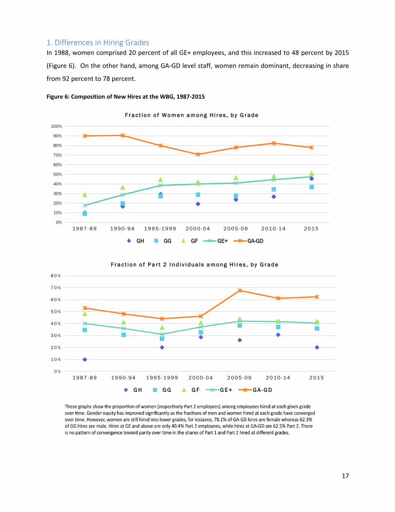
Over the period of our data, the fractions of men and women hired at each grade have converged.

However, even in 2015 women were hired into lower grades on average: 78.1% of GA-GD hires were

female whereas 62.3% of GG hires were male. Further, the historical differences in hiring created a

pipeline to higher paid jobs that contain more men. Compositional differences between Part 1 and Part 2

are qualitatively similar to those between men and women. Hires at GE and above are 40.4% Part 2

employees, while hires at GA-GD are 62.5% Part 2. In contrast to the gender differences, however, there

is no pattern of convergence toward parity over time in the shares of Part 1 and Part 2 staff hired at

different grades.

Consistent with these patterns, the decomposition of the aggregate gap shows that 76% of the aggregate

gender gap in 2015 and 61% of the aggregate country part gap in 2015 can be attributed to differences in

grade composition at entry. In addition, differences in salary growth and differences in entry salaries

account for 12% of the aggregate gap across men and women and 16% across Part 1 and Part 2 staff.

Finally, attrition is a more important contributor (14%) for the aggregate gap across Part 1 and Part 2

employees relative to the aggregate gap across women and men (1%).

Career gaps varied across entry grades, which is an important finding in itself. In grades GE and GG, 15

years after joining the WBG any existing gaps in salaries by sex or nationality were small. In all other grades

besides GF, there were insufficient hires in each year for every subgroup to offer meaningful estimates.

For instance, the largest number of men in the GA-GD cohort were hired in grade GB. But even there, only

209 men were hired (an average of 8 men per year) over the duration of our data and there were 12 years

with 3 or fewer men hired into this grade. Similarly, for grade GH, there were 11 years with fewer than 5

women hired into the grade; for higher grades, the numbers were even smaller.

9 As a comparison, the aggregate gender pay gap in the United States declined from 26 cents on the dollar in 1989 to 20.7 cents

on the dollar in 2010 (Blau and Kahn, 2016).

5

For employees who entered at GF, there were both sizeable salary differences and sufficient sample to

further decompose career gaps. We therefore focus our decomposition of the career gap for staff who

joined the WBG in grade GF between 1987 and 2001. This results in a sample of 1,763 staff who had been

hired as a GF in 2001 or earlier, representing 37.1 percent of all hires at grades GE+ among those cohorts.

Relative to male Part 1 employees, in this sample 15 years after entering the WBG, the annual salary of

female Part 1 employees was $5,036 lower. It was $5,178 lower for male Part 2 employees and $4,139

lower for female Part 2 employees. In percentage terms, for every dollar that male Part 1 employees (who

entered as a GF) earned after 15 years, female Part 1 employees earned 96.52 cents, male Part 2

employees earned 96.42 cents and female Part 2 employees earned 97.14 cents. Our decomposition

results indicate that the bulk of these differences is explained by differences in salary growth (rather than

entry salaries or attrition), which reflects a longer lead time for promotions to grades GG and GH.

Although the data thus show a career gap after 15 years for those who entered as GF, we should caution

that attrition from the WBG may confound any interpretation of this gap. About 8-10 percent of staff

leave the WBG every year, and therefore within 7-9 years, half of original staff hires exit the sample. The

decomposition analysis assumes that, had they not left the WBG, leavers and stayers in the same cohort

would receive the same salaries, conditional on their last salary and entry grade. Our analysis did not find

differences—in the means or distributions of either performance or salaries—of stayers versus leavers,

but it could be sensitive to that assumption.10

These relatively modest career gaps are somewhat surprising given previous analysis by Filmer et al.

(2005), which showed a consistent salary premium for Part 1 men compared to women and Part 2

employees.11 It also runs contrary to the perceptions of staff at the institution. To address this concern,

we first re-examined the Filmer et al. (2005) results and found that the gender salary gap becomes small

in their analysis once starting grades are accounted for—information that was not incorporated in the

Filmer et al. (2005) salary decomposition. The results presented here are therefore consistent with those

of Filmer et al. (2005) as both our analysis and theirs points to entry grades as a critical determinant of

current salary gaps.

10 In addition to examining compensation metrics prior to staff leaving the WBG, we also tried to follow-up a small group of (randomly) selected staff who had left the Bank and tracked down where they were currently employed using Social Networks such as Facebook and LinkedIn. Current employment appears to be very diverse, with some staff employed in other international organizations, academia, the public or private sector, or staying on in a consultancy role at the WBG. 11 Filmer et al. (2005) used a cross-section of salaries among what were in 1997 known as professional staff. They identified salary deficits for women and Part 2 employees at the World Bank, only half of which could be explained by differences in staff characteristics.

6

We then examined whether the smaller contributions of entry salaries and salary growth to the aggregate

gap reflects a flat compensation system with a strong preference for equity that seeks to close gaps where

they exist. For instance, at the WBG, the compensation methodology seeks to promote equity within each

grade by accelerating increases for those staff positioned below the midpoint and moderating for staff

positioned above the midpoint, so that over time, equal performance is compensated in an equitable way.

This is supported by the 2015 introduction of a four-zone salary band.

In fact, we found that salary responds strongly to performance ratings at the WBG. Among the cohort of

GF entrants between 2000 and 2005, staff in the lowest performance decile gained 26 percent in real

salaries over a 10-year period while those in the highest performance decile gained 83 percent. We also

did not find evidence for the systematic application of informal management practices that could limit

performance-related pay increases, such as not awarding staff the highest performance rating in two

successive years. The hiring and compensation system at the WBG is thus reasonably successful at

restricting subgroup differences among staff hired in the same grade, while maintaining salary incentives

for high performance. However, it is not as successful in retaining high performing staff as exits from the

institution are not correlated with historical performance.

Our econometric approach to diversity and inclusion issues in a large firm contrasts with a complementary

human resource approach, where individual cases are examined on the basis of cross-sectional data to

ensure compliance with equal pay policies. Our attempt here is to apply the tools available in the labor

literature to the internal labor market of a single firm to generate policy insights for compensation policies

in such environments. The combination of a data-based simulation approach thus bridges the large

literature on subgroup differences in the labor market and growing interest in the organization of large

firms.

In addition, the empirical approach we follow also complements, but is conceptually different from, a

literature that decomposes wage differences across subgroups into those arising from employee

characteristics and those arising from the returns to these characteristics. Given the longitudinal data

available to us, our decomposition allows us to identify the sources of wage gaps and provides a starting

point for further institutional efforts. For instance, relative to the cross-sectional data used by Filmer et

al. (2005), these data allow us to incorporate employee turnover and pipeline effects (historical hiring will

affect gaps today), which could mask or artificially amplify salary gaps in cross-sections. One key finding is

that pay gaps arise at different points in staff careers depending on their entry grade. The organizational

structure that leads to different gaps in different grades merits further debate and it is in understanding

7

these very specific gaps that incorporating employee characteristics will likely become a critical part of

the analytical work.12

The remainder of this document is as follows. In Section II, we discuss the construction of the data set and

broad patterns in the data that illustrate the institutional context for our findings. Section III provides the

key descriptive findings on salary gaps by gender and nationality in terms of each individual contributor—

composition, entry salaries, salary growth and turnover. Section IV discusses the results of our dynamic

accounting framework, which allows us to decompose the aggregate and career gaps into each of their

sub-components using simulations. Section V concludes.

II. Data The World Bank Group's Human Resource Longitudinal Database was constructed in order to better

understand salary dynamics and career differences across subgroups such as gender and nationality. The

data set is structured in a panel from 1987 to 2015 with staff uniquely identified through a universal

personnel identifier (UPI) that never changes for an individual, even across disjointed employment spells.

The data are gathered from two human resource databases at the WBG—PeopleSoft/Business

Intelligence and Talent Management—with data from each year taken as a snapshot on June 30.

PeopleSoft/Business Intelligence contains information on the staff’s universal personnel identified (UPI);

compensation and benefits (e.g. salaries); personal backgrounds (e.g. gender, age); professional situation

(e.g. professional grade); location (e.g. HQ or country-office based) and role and movements within the

organization (e.g. promotions and lateral moves). In addition to these, information on the yearly

performance rating (SRIs), which is available from 2000 onwards, is drawn from the Talent Management

database.

Unfortunately, PeopleSoft does not contain reliable data going back to 1987 and multiple changes in the

WBG ranging from types and grades of employees to corrections in the employment spells had to be

carefully dealt with. A brief description of the types of employees and how they have changed over time

is necessary to interpret the results; the accompanying data Appendix and codebook provides further

details.

The most important broad distinction between types of employees at the WBG is between staff members

and consultants. Our data contain all staff members. The data set has no information on Short-Term

12 We caution that the WBG’s data on pre-entry characteristics of staff are incomplete. Some of this is because we have staff members in our data who were hired as far back as 1955, but this is also because pre-entry data on staff are not standardized. They are based on individual CVs submitted by staff and the information contained in these CVs can vary dramatically. As one example, the variable that captures the highest educational degree is missing for 55 percent of staff in the data.

8

Consultants, who can range from people working exclusively at the WBG to those on short contracts, but

with permanent jobs at other institutions. Although there is considerable movement of staff from

consultancy to staff contracts, the data on consultants are too limited for inclusion in our analysis.

Among staff members, the WBG grades run from GA to GL (the president of the WBG). Grades GA-GD are

the grade levels for Administrative and Client Services (ACS) staff. GE corresponds to analyst-level. GF and

GG contain the bulk of professional technical staff. Staff in the GH level, the first leadership position at

the WBG, can be either in a technical or managerial role. GI (Director) through GK (Vice Presidents) and

GL (President) refer to senior management positions. Staff entering the WBG can do so through multiple

channels. Staff can be recruited through international recruitment by different units, which advertise

positions and hire new employees at the relevant grade level. Staff can be hired through local recruitment,

which does not include international benefits. In addition, staff can also be recruited through the “Young

Professional” process, which is the flagship recruitment program of the institution.13

Apart from these grades, our data also contain information on employees with “Unassigned or Ungraded”

grades. These are of two types. First, a small number are staff outside the salary and promotion structure

of the WBG, such as executive directors and their advisers. Second, prior to a reform in 1998 (which we

discuss in Footnote 15 below) a large fraction of employees without grades were “long-term consultants”,

who were not considered staff members but nevertheless held full time jobs at the WBG. With the reform,

many of them were converted to graded employees, and a new category of ungraded employees with

specific 2-3 year contracts was introduced called Extended-Term Consultants. In 2016, these posts were

abolished as well; our data stop a year prior to this last change. Before 1999, therefore, the unclassified

grade was a highly heterogeneous category, including country managers and Executive Directors (EDs).

After 1999, the grade became more homogeneous, with most regular staff being slotted into normal grade

levels.

1. Sample Even though the WBG has more than 100 country offices, we restricted our sample to staff in the

Washington D.C. headquarters hired on a US dollar salary plan, commonly known as “internationally

recruited staff”. The main reason for the restriction is the substantial country-specific expertise required

to convert local salaries to dollar equivalents. Given the starting date of 1987 in our data, the dissolution

of the Soviet Union and the emergence of local currencies, the emergence of the euro and the dissolution

13 Since 2015, there is an additional recruitment program at the GE-level called the Analyst Program. Before that, there was a multitude of different youth recruitment programs which were phased in and out over time. Most of these were graded as Unclassified.

9

of local currencies as well as multiple hyperinflations through the period of our data in countries ranging

from Turkey to Ecuador all need to be addressed on a case-by-case basis. While this salary conversion is

possible, it lies outside the scope of the current project and requires close collaboration between country

units and the relevant global practices at the WBG. This restriction becomes particularly worrisome for

our ability to examine Part 1 versus Part 2 differences in the latter period of our sample as the fraction of

local hires increases from 7.4 percent to 37.8 percent over the time period of our data.

Despite the decline in sample resulting from this restriction, our data set continues to represent a large

number of nationalities and citizens of Part 2 countries.14 Figure 1 charts staff nationalities among new

international hires in 1990, 2000 and 2010. In all years, more than 60 countries were represented in

international hiring and over time and the dominance of the top 5 countries (United States, India, Great

Britain, France and the Philippines in 1990) declined from 54 percent of all international hires in 1990 to

44 percent in 2010.15

Figure 1: Diversity in Terms of Nationality at the WBG

14 Staff may change their citizenship after arriving at the WBG. The most common citizenship change will be to U.S., and we find 173 such cases in our data among 30,763 staff members. Our understanding is that this low number is driven by the loss of benefits when people become U.S. citizens, combined with the ability to obtain a Green Card on exiting the WBG after 15 years of employment. 15 One way that social scientists summarized diversity in populations is through “diversity indices”. For instance, the Blau diversity index is the expected proportion of people who would be from different groups if two members were picked randomly from the population. A diversity index of 0 implies that there is no diversity in the population while 1 implies that no two people are from the same group. At the WBG, the Blau Diversity Index was already very high at 0.87 in 1990 and by 2010, it had increased even further to 0.92.

Other

46%

US

34%

IN

7%

GB

5%

FR

4%

PH

4%

1987-1995

Other US IN GB FR PH

Other

54%

US

32%

IN

6%

GB

4%

FR

4%

1996-2005

Other US IN GB FR

Other

58%

US

25%

IN

6%

FR

4%

GB

4%

DE

3%

2006-2015

Other US IN FR GB DE

10

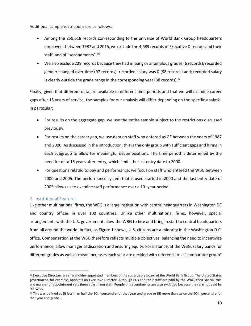
Additional sample restrictions are as follows:

Among the 259,618 records corresponding to the universe of World Bank Group headquarters

employees between 1987 and 2015, we exclude the 4,689 records of Executive Directors and their

staff, and of “secondments”.16

We also exclude 229 records because they had missing or anomalous grades (6 records); recorded

gender changed over time (97 records); recorded salary was 0 (88 records) and; recorded salary

is clearly outside the grade range in the corresponding year (38 records).17

Finally, given that different data are available in different time periods and that we will examine career

gaps after 15 years of service, the samples for our analysis will differ depending on the specific analysis.

In particular:

For results on the aggregate gap, we use the entire sample subject to the restrictions discussed

previously.

For results on the career gap, we use data on staff who entered as GF between the years of 1987

and 2000. As discussed in the introduction, this is the only group with sufficient gaps and hiring in

each subgroup to allow for meaningful decompositions. The time period is determined by the

need for data 15 years after entry, which limits the last entry date to 2000.

For questions related to pay and performance, we focus on staff who entered the WBG between

2000 and 2005. The performance system that is used started in 2000 and the last entry date of

2005 allows us to examine staff performance over a 10- year period.

2. Institutional Features Like other multinational firms, the WBG is a large institution with central headquarters in Washington DC

and country offices in over 100 countries. Unlike other multinational firms, however, special

arrangements with the U.S. government allow the WBG to hire and bring in staff to central headquarters

from all around the world. In fact, as Figure 1 shows, U.S. citizens are a minority in the Washington D.C.

office. Compensation at the WBG therefore reflects multiple objectives, balancing the need to incentivize

performance, allow managerial discretion and ensuring equity. For instance, at the WBG, salary bands for

different grades as well as mean increases each year are decided with reference to a “comparator group”

16 Executive Directors are shareholder-appointed members of the supervisory board of the World Bank Group. The United States government, for example, appoints an Executive Director. Although EDs and their staff are paid by the WBG, their special role and manner of appointment sets them apart from staff. People on secondments are also excluded because they are not paid by the WBG. 17 This was defined as (i) less than half the 10th percentile for that year and grade or (ii) more than twice the 90th percentile for that year and grade.

11

that includes a mix of other international organizations, private sector firms and public sector salaries.

However, to allow for managerial discretion and performance incentives, compensation bands within

each grade are quite wide and in theory, raises can vary substantially around the average increase,

depending both on the performance rating of the employee in the last year as well as their relative

position within the salary band for their grade. To promote equity, employees with salaries above the

midpoint of their grade receive a lower raise for the same level of performance.

These practices have not remained static over the period of our data. In fact, multiple institutional changes

and HR policies have been enacted to further one or more of these objectives. These, in turn could have

affected hiring and turnover as well as the salary structure.18 It is therefore useful to examine basic

summary statistics that deepen our understanding of the underlying dynamics in the data.

3. Summary Statistics A first characterization of the data is in terms of compositional changes. Figure 2 shows that over the

period of our data, there was a secular increase in the fraction of GE+ level staff as a fraction of total staff

from 64 percent in 1987 to 85 percent in 2015, consistent both with increasing automatization of routine

tasks and shifting of routine tasks from GA-GD to GE+ staff.19 The proportional increase in GE+ staff was

primarily in the technical grades of GE, GF and GH; no change was seen in the proportion of managers to

staff between the years of 2000 and 2015.20

18 An important policy change was a reform in 1998 that changed the pension regimes (from defined benefits to a combination of defined benefit and defined contribution), the grading system (from ‘narrow’ to ‘broad banding’ thus shifting the WBG from smaller bands and more frequent promotions to larger bands with fewer promotions) and, importantly for our analysis, eliminated long-term consultant contracts. Appendix Figure 1 shows all new hires between 1990 and 2005 at the WBG for ungraded, GA-GD and GE+ staff. The term “ungraded” are those with “unassigned” or “unclassified” grades at the institution—prior to 1998 these included staff on long-term consultant contracts and country managers. After 1998 these were mostly (see Technical Appendix 1) staff hired on Extended Term Consultant or Extended Term Temporary contracts with a fixed duration. New hiring in the ungraded category collapsed immediately after the reform and then picked up, but at much lower levels than before with the coming of ETCs and ETTs. Many ungraded staff were converted to “regular” staff at different grade-levels where there is a corresponding spike in “new” hires at those grades in 2008: 59 percent of those who were ungraded in 1998 were converted over the next 3 years. Managers appeared to have been forward-looking in their hiring decisions with a “dip” in regular hiring and a large increase in ungraded hiring prior to the reform: between 1987 and 1998, the fraction of all employees who are ungraded rises from 11.9 percent to 29.3 percent. Prior to the reform, the salary distribution among the ungraded is quite wide with a difference of over $72,000 (285%) between those in the bottom and top 10% in 1997. In our analysis, we always treat those who were ungraded prior to 1987 as separate and then re-analyze them as if they had no history with the WBG if we see them as converted in 1998. That is, we treat a new employee at the institution who enters (say) as GF in 1998 precisely the same as those who were converted from ungraded to GF. We have checked, in sensitivity analysis, whether this is a valid assumption and can confirm that the experiences of these staff are no different from those of new entrants at that grade in 1998. 19 There are small differences in the year-to-year changes depending on how we treat the ungraded staff prior to the 1998 reform. Here we exclude the ungraded staff from the figure, which implicitly assumes the fraction of professional to support staff in the ungraded and graded staff prior to the 1998 reform was the same. 20 The data do not allow us to identify managers prior to 2000.

12

Figure 2: Grade Composition at the WBG between 1987 and 2015

A second characterization recognizes that the composition of employees depends both on hiring and exits.

Figure 3 plots annual exits from the institution as a percentage of regular staff, excluding staff exits due

to mandatory retirement. Exits at the WBG cycle around an average of 9 percent a year.21 Exits were

higher in 1987 and 1988 and then declined to a low of 6 percent before rising again to a peak with a large

institutional reform in 1998 followed by a subsequent trough of 6 percent in 2000. Since then exits

increased again with an 11 percent exit rate in 2015, the last year of our data. One hypothesis consistent

with these patterns is that institutional reforms such as those seen in 1998 and 2012-2013 accelerate the

exits of those who would have left within 2-3 years. Consequently, exits peak in reform years (which are

usually associated with new presidential terms) but then drop because reforms bring exits “forward”. A

second hypothesis—more clearly seen in the first half of our data—is that exits track economic

performance in the U.S., rising when the economy is strong. Regardless of the specific hypothesis, the 9%

exit rate implies that 50% of staff leave the institution every 8 years. These high rates of attrition leave

substantial room for interpreting the remaining salary gaps of those who choose to remain at the

21 Of independent interest, higher exits are not associated with higher age at exit with a mean age at exit of 43.5 years

0

10

20

30

40

50

60

70

80

90

100

Sh

are

of

Em

plo

yee

s (

%)

GA-GD GE-GH GE-GH Non-Managers GE-GH Managers GI+

13

institution for 15 years or more—and are clearly a significant limitation when we apply the tools of cohort

analysis to a single firm.22

Figure 3: Exit Rates from the WBG between 1987 and 2015

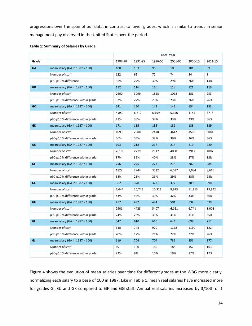
A final characterization of the data is in terms of salaries. Table 1 shows the mean real salaries of

employees at each grade over time and to focus on changes, we compare all salaries to a base of 100 for

grade GA in 1987.23 To preserve anonymity, we leave blank the cells where there are too few employees

and do not present results for grade GK. The table first demonstrates considerable variation in salaries

within each grade. Typically, there is a difference of 20-40% between the 10th percentile and the 90th

percentile of the within-grade salary distribution. Second, salaries in higher grades exhibit large

22 If b is the exponential decay rate, x the initial stock of employees and t the number of years, then the existing employee stock with halve when xbt=x/2 or, tln(b)=ln(0.5) or t = ln(0.5)/ln(b). With an attrition rate of 9%, b=0.91 yielding 8 years for halving the employee stock. 23 We use the consumer price index for the U.S. to deflate nominal salaries—note that price increases in the Baltimore-Washington area have been higher than for the U.S. as a whole, so using the BW CPI will lower real wage increases further over the period of our data.

5

6

7

8

9

10

11

12

13

Sh

are

of

Em

plo

yee

s (

%)

Wo

lfe

nso

hn

Zo

ellic

k

Kim

Co

na

ble

Pre

sto

n

Wo

lfo

wit

z

14

progressions over the span of our data, in contrast to lower grades, which is similar to trends in senior

management pay observed in the United States over the period.

Table 1: Summary of Salaries by Grade

Fiscal Year

Grade

1987-90 1991-95 1996-00 2001-05 2006-10 2011-15

GA mean salary (GA in 1987 = 100) 100 103 96 100 101 99

Number of staff 122 62 72 74 34 8

p90-p10 % difference 36% 27% 30% 29% 26% 13%

GB mean salary (GA in 1987 = 100) 112 116 116 118 121 119

Number of staff 2600 3099 1828 1068 381 253

p90-p10 % difference within grade 32% 27% 25% 23% 26% 26%

GC mean salary (GA in 1987 = 100) 141 150 148 149 154 153

Number of staff 4,859 6,212 6,159 5,156 4155 3718

p90-p10 % difference within grade 41% 38% 38% 33% 33% 36%

GD mean salary (GA in 1987 = 100) 171 185 185 182 188 189

Number of staff 1093 2088 2478 3642 3506 3084

p90-p10 % difference within grade 36% 33% 38% 39% 36% 36%

GE mean salary (GA in 1987 = 100) 193 218 217 214 219 220

Number of staff 2618 2719 2917 4000 3917 4007

p90-p10 % difference within grade 37% 32% 40% 38% 37% 33%

GF mean salary (GA in 1987 = 100) 256 275 273 278 282 284

Number of staff 1822 2944 3522 6,017 7,084 8,615

p90-p10 % difference within grade 33% 23% 26% 29% 28% 28%

GG mean salary (GA in 1987 = 100) 362 378 372 377 389 390

Number of staff 7,644 10,746 10,323 9,973 11,813 13,842

p90-p10 % difference within grade 43% 42% 39% 32% 33% 36%

GH mean salary (GA in 1987 = 100) 457 492 484 501 534 539

Number of staff 2901 4428 5407 6,161 6,741 8,008

p90-p10 % difference within grade 24% 26% 33% 31% 31% 35%

GI mean salary (GA in 1987 = 100) 547 610 610 644 698 712

Number of staff 548 743 920 1168 1160 1224

p90-p10 % difference within grade 20% 17% 21% 22% 22% 26%

GJ mean salary (GA in 1987 = 100) 619 706 704 782 851 877

Number of staff 69 100 160 188 152 163

p90-p10 % difference within grade 23% 9% 16% 19% 17% 17%

Figure 4 shows the evolution of mean salaries over time for different grades at the WBG more clearly,

normalizing each salary to a base of 100 in 1987. Like in Table 1, mean real salaries have increased more

for grades GI, GJ and GK compared to GF and GG staff. Annual real salaries increased by 3/10th of 1

15

percent between 1987 and 2014 among GB-GD and GG staff, 7/10th of 1 percent for GE and GH level staff

and 1.1 to 1.6 percent for GI-GK level staff.24

Figure 4: Salary Trends for Staff at the WBG, 1987-2015

Each of these “macro-changes” over the period of our data can affect the salary gap across subgroups.

For instance, the decline in GA-GD level staff, who are predominantly women in jobs with lower salaries

implies that the average salary of women relative to men will rise in the institution. Similarly, differences

in the profile of staff leaving the WBG will affect the salaries of those who remain. Finally, differential

increases in salaries for different grades can affect both aggregate and career gaps. First, as GA-GD staff

tend to be women, their lower salary growth over time will imply that the aggregate gap will also increase.

Second, staff are promoted over time. If men are promoted faster to GH (for instance) relative to women

and GH salaries are growing faster, this will again induce an increase in both the aggregate and career

24 These are salaries of all staff in a given grade, and thus include tenure effects; with zero turnover, salaries will grow with experience. A second option, in Appendix Figure 2 focuses just on entry-level salaries for different grades over this time period. Like in Figure 4, with the exception of GI+ staff, real entry salaries have increased slowly over this period with the largest increases of 15-20% for GH level staff.

100

110

120

130

140

150

160

1987 1990 1995 2000 2005 2010 2014

Ave

rage

Re

al S

ala

ry (

19

87

=1

00

)

GB

GC

GD

GE

GF

GG

GH

GI

GJ

GK

16

gaps over time.25 Taken as aggregates, there is considerable room both in the composition of employees

and how they are compensated for differences by subgroups to arise. We turn to this next.

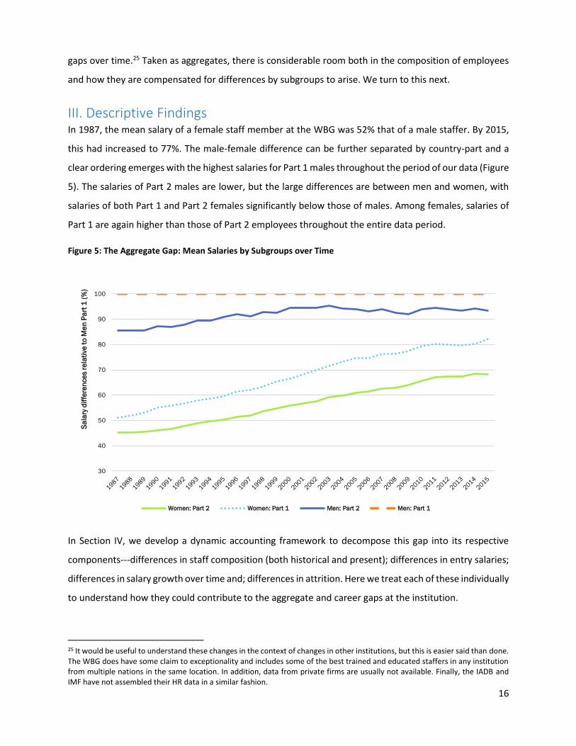
III. Descriptive Findings In 1987, the mean salary of a female staff member at the WBG was 52% that of a male staffer. By 2015,

this had increased to 77%. The male-female difference can be further separated by country-part and a

clear ordering emerges with the highest salaries for Part 1 males throughout the period of our data (Figure

5). The salaries of Part 2 males are lower, but the large differences are between men and women, with

salaries of both Part 1 and Part 2 females significantly below those of males. Among females, salaries of

Part 1 are again higher than those of Part 2 employees throughout the entire data period.

Figure 5: The Aggregate Gap: Mean Salaries by Subgroups over Time

In Section IV, we develop a dynamic accounting framework to decompose this gap into its respective

components---differences in staff composition (both historical and present); differences in entry salaries;

differences in salary growth over time and; differences in attrition. Here we treat each of these individually

to understand how they could contribute to the aggregate and career gaps at the institution.

25 It would be useful to understand these changes in the context of changes in other institutions, but this is easier said than done. The WBG does have some claim to exceptionality and includes some of the best trained and educated staffers in any institution from multiple nations in the same location. In addition, data from private firms are usually not available. Finally, the IADB and IMF have not assembled their HR data in a similar fashion.

30

40

50

60

70

80

90

100

Sa

lary

dif

fere

nce

s r

ela

tive

to

Me

n P

art

1 (

%)

Women: Part 2 Women: Part 1 Men: Part 2 Men: Part 1

17

1. Differences in Hiring Grades In 1988, women comprised 20 percent of all GE+ employees, and this increased to 48 percent by 2015

(Figure 6). On the other hand, among GA-GD level staff, women remain dominant, decreasing in share

from 92 percent to 78 percent.

Figure 6: Composition of New Hires at the WBG, 1987-2015

0%

10%

20%

30%

40%

50%

60%

70%

80%

90%

100%

1 9 8 7 - 8 9 1 9 9 0 - 9 4 1 9 9 5 - 1 9 9 9 2 0 0 0 - 0 4 2 0 0 5 - 0 9 2 0 1 0 - 1 4 2 0 1 5

F r a c t i o n o f W o m e n a m o n g H i r e s , b y G r a d e

GH GG GF GE+ GA-GD

0 %

1 0 %

2 0 %

3 0 %

4 0 %

5 0 %

6 0 %

7 0 %

8 0 %

1 9 8 7 - 8 9 1 9 9 0 - 9 4 1 9 9 5 - 1 9 9 9 2 0 0 0 - 0 4 2 0 0 5 - 0 9 2 0 1 0 - 1 4 2 0 1 5

F r a c t i o n o f P a r t 2 I n d i v i d u a l s a m o n g H i r e s , b y G r a d e

G H G G G F G E + G A - G D

18

It is worth emphasizing that in most grades, hiring from all subgroups was so low that sufficient samples

for analysis at the grade-level are hard to obtain.26 Figure 7 shows hiring in each year for Grades GB and

GH; among grades GA to GD, GB has the highest number of male hires and among grades GH+, GH has

the highest number of female hires over the period of our data. Even here, the number of male hires (GB)

and female hires (GH) is small, exceeding 10 hires in only a couple of years (GB) and never more than 10

for GH. There are several years where fewer than 2 GB males or 2 GH males are hired. Figure 7 also shows

new GF and GG hires. Again, there is a female disadvantage (more so for GG) but the gap narrows over

the period of our data and the number of hires across males and females is now sufficiently large that we

can recover a sizeable sample by aggregating a small number of years into a single cohort analysis.

For the decomposition exercise, the stock of employees at different grades reflects both pipeline effects

and new hiring. For example, suppose an employee can rise to GH only after 12-15 years of service at the

Bank if starting as a GF and 5-7 years if starting as GG. In that case, if GHs are predominantly promoted

within the institution, they will be naturally constrained by the number of GFs and GGs 7-15 years in the

past. But in 2000, there were 1,112 female GFs and GGs, relative to just under 2,000 male GFs and GGs.

Although a crude measure of the pipeline (where tenure effects, exits and grade-year interactions will all

become relevant), the example emphasizes that that there is a long lead time between policy changes

and current staffing patterns. These lead times will be longer at the higher grades and will be longer if

promotions rather than external hires form the bulk of employees at these higher grades.

26 There were 260 male GF’s, 1634 male GGs and 673 male GH’s in 1987 relative to 177 (GF), 285 (GG) and 25 (GH) females. In 1987, there were 684 female GBs, 1074 GCs and 190 GDs compared to 84 (GB), 114 (GC) and 52 (GD) for men. By 2015, the number of female GBs and GCs had reduced to 26 and 587 while GDs had increased to 469. And there were only 12 male GBs, 101 male GCs and 84 male GDs.

19

Figure 7: Number of Female and Male New Hires in Grades GB, GH and GF, GG: 1988-2015

0

20

40

60

80

100

120

140

160

180

200

19

88

19

89

19

90

19

91

19

92

19

93

19

94

19

95

19

96

19

97

19

98

19

99

20

00

20

01

20

02

20

03

20

04

20

05

20

06

20

07

20

08

20

09

20

10

20

11

20

12

20

13

20

14

20

15

No

. o

f P

eo

ple

Hir

ed

Male Female

0

5

10

15

20

25

30

35

40

45

19

88

19

89

19

90

19

91

19

92

19

93

19

94

19

95

19

96

19

97

19

98

19

99

20

00

20

01

20

02

20

03

20

04

20

05

20

06

20

07

20

08

20

09

20

10

20

11

20

12

20

13

20

14

20

15

No

. o

f P

eo

ple

Hir

ed

Male Female

0

20

40

60

80

100

120

140

160

180

200

19

88

19

89

19

90

19

91

19

92

19

93

19

94

19

95

19

96

19

97

19

98

19

99

20

00

20

01

20

02

20

03

20

04

20

05

20

06

20

07

20

08

20

09

20

10

20

11

20

12

20

13

20

14

20

15

No

. o

f P

eo

ple

Hir

ed

Male Female

0

50

100

150

200

250

19

88

19

89

19

90

19

91

19

92

19

93

19

94

19

95

19

96

19

97

19

98

19

99

20

00

20

01

20

02

20

03

20

04

20

05

20

06

20

07

20

08

20

09

20

10

20

11

20

12

20

13

20

14

20

15

No

. o

f P

eo

ple

Hir

ed

Male Female

20

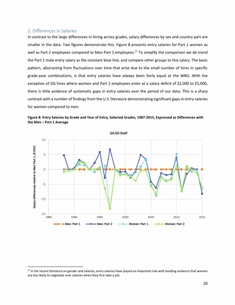
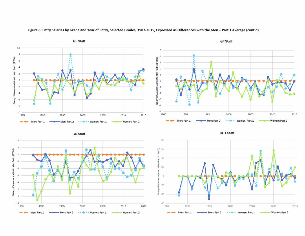
2. Differences in Salaries In contrast to the large differences in hiring across grades, salary differences by sex and country part are

smaller in the data. Two figures demonstrate this. Figure 8 presents entry salaries for Part 1 women as

well as Part 2 employees compared to Men Part 1 employees.27 To simplify the comparison we de-trend

the Part 1 male entry salary as the constant blue-line, and compare other groups to this salary. The basic

pattern, abstracting from fluctuations over time that arise due to the small number of hires in specific

grade-year combinations, is that entry salaries have always been fairly equal at the WBG. With the

exception of GG hires where women and Part 2 employees enter at a salary deficit of $2,000 to $5,000,

there is little evidence of systematic gaps in entry salaries over the period of our data. This is a sharp

contrast with a number of findings from the U.S. literature demonstrating significant gaps in entry salaries

for women compared to men.

Figure 8: Entry Salaries by Grade and Year of Entry, Selected Grades, 1987-2015, Expressed as Differences with the Men – Part 1 Average

27 In the recent literature on gender and salaries, entry salaries have played an important role with building evidence that women are less likely to negotiate over salaries when they first take a job.

-15

-10

-5

0

5

10

1985 1990 1995 2000 2005 2010 2015

Sa

lary

dif

fere

nce

s r

ela

tive

to

Me

n P

art

1 (

$'0

00

)

GA-GD Staff

Men: Part 1 Men: Part 2 Women: Part 1 Women: Part 2

21

Figure 8: Entry Salaries by Grade and Year of Entry, Selected Grades, 1987-2015, Expressed as Differences with the Men – Part 1 Average (cont’d)

-10

-8

-6

-4

-2

0

2

4

6

8

10

1985 1990 1995 2000 2005 2010 2015

Sa

lary

dif

fere

nce

s r

ela

tive

to

Me

n P

art

1 (

$'0

00

)

GE Staff

Men: Part 1 Men: Part 2 Women: Part 1 Women: Part 2

-5

-4

-3

-2

-1

0

1

2

3

4

5

1985 1990 1995 2000 2005 2010 2015

Sa

lary

dif

fere

nce

s r

ela

tive

to

Me

n P

art

1 (

$'0

00

)

GF Staff

Men: Part 1 Men: Part 2 Women: Part 1 Women: Part 2

-14

-12

-10

-8

-6

-4

-2

0

2

4

1985 1990 1995 2000 2005 2010 2015

Sa

lary

dif

fere

nce

s r

ela

tive

to

Me

n P

art

1 (

$'0

00

)

GG Staff

Men: Part 1 Men: Part 2 Women: Part 1 Women: Part 2

-60

-40

-20

0

20

40

60

80

1985 1990 1995 2000 2005 2010 2015

Sa

lary

dif

fere

nce

s r

ela

tive

to

Me

n P

art

1 (

$'0

00

)

GH+ Staff

Men: Part 1 Men: Part 2 Women: Part 1 Women: Part 2

22

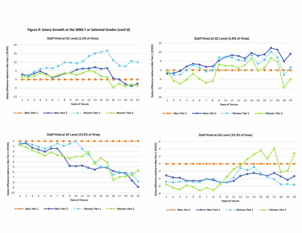
Figure 9 shows salary growth for employees at the WBG. The horizontal axis in each figure shows the

number of years that the staff has worked at the WBG, and we aggregate staff with the same number of

tenure years, irrespective of the year in which they joined the institution.28 As with entry salaries, Grades

GC and GE appear to have little difference in salary growth over time. In contrast, Grades GB and GF show

clear declines over time, reaching a $10,000 difference in annual salary after 20 years for GF employees.

Grade GG starts off with a salary deficit for all groups relative to Part 1 males, also seen in the salary at

entry, but there appears to be some catch-up over time. More generally, Figure 10 shows the existing

salary gaps after 15 years of tenure at the WBG, highlighting the larger deficits among staff who entered

as GB or GF, but not GC, GD, GE or GG.

Figure 9: Salary Growth at the WBG for Selected Grades

28 For instance, people who joined in 1990 and 1995 will have 10 years of tenure in 2000 and 2005. Therefore, the salary pertaining to (say) 10 years of tenure is the average salary of those who joined in 1990, but observed in 2000 and those who joined in 1995, but observed in 2005.

-8

-7

-6

-5

-4

-3

-2

-1

0

1

2

1 2 3 4 5 6 7 8 9 10 11 12 13 14 15 16 17 18 19 20

Sa

lary

dif

fere

nce

re

lati

ve

to

Me

n P

art

1 (

$'0

00

)

Years of Tenure

Staff Hired at GB Level (31.9% of Hires)

Men: Part 1 Men: Part 2 Women: Part 1 Women: Part 2

23

Figure 9: Salary Growth at the WBG f or Selected Grades (cont’d)

-10

-5

0

5

10

15

20

1 2 3 4 5 6 7 8 9 10 11 12 13 14 15 16 17 18 19 20

Sa

lary

dif

fere

nce

re

lati

ve

to

Me

n P

art

1 (

$'0

00

)

Years of Tenure

Staff Hired at GC Level (2.2% of Hires)

Men: Part 1 Men: Part 2 Women: Part 1 Women: Part 2

-15

-10

-5

0

5

10

15

1 2 3 4 5 6 7 8 9 10 11 12 13 14 15 16 17 18 19 20

Sa

lary

dif

fere

nce

re

lati

ve

to

Me

n P

art

1 (

$'0

00

)

Years of Tenure

Staff Hired at GE Level (4.8% of Hires)

Men: Part 1 Men: Part 2 Women: Part 1 Women: Part 2

-10

-9

-8

-7

-6

-5

-4

-3

-2

-1

0

1 2 3 4 5 6 7 8 9 10 11 12 13 14 15 16 17 18 19 20

Sa

lary

dif

fere

nce

re

lati

ve

to

Me

n P

art

1 (

$'0

00

)

Years of Tenure

Staff Hired at GF Level (23.5% of Hires)

Men: Part 1 Men: Part 2 Women: Part 1 Women: Part 2

-8

-6

-4

-2

0

2

4

6

1 2 3 4 5 6 7 8 9 10 11 12 13 14 15 16 17 18 19 20

Sa

lary

dif

fere

nce

re

lati

ve

to

Me

n P

art

1 (

$'0

00

)

Years of Tenure

Staff Hired at GG Level (33.3% of Hires)

Men: Part 1 Men: Part 2 Women: Part 1 Women: Part 2

24

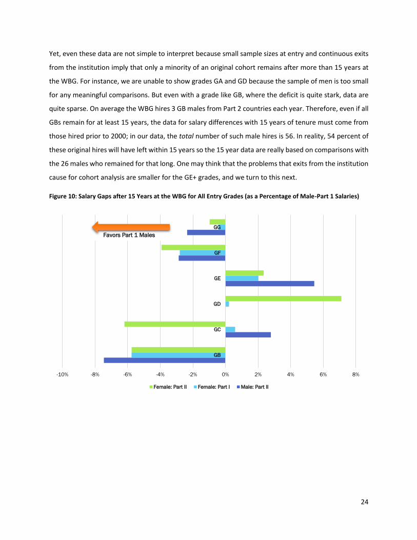
Yet, even these data are not simple to interpret because small sample sizes at entry and continuous exits

from the institution imply that only a minority of an original cohort remains after more than 15 years at

the WBG. For instance, we are unable to show grades GA and GD because the sample of men is too small

for any meaningful comparisons. But even with a grade like GB, where the deficit is quite stark, data are

quite sparse. On average the WBG hires 3 GB males from Part 2 countries each year. Therefore, even if all

GBs remain for at least 15 years, the data for salary differences with 15 years of tenure must come from

those hired prior to 2000; in our data, the total number of such male hires is 56. In reality, 54 percent of

these original hires will have left within 15 years so the 15 year data are really based on comparisons with

the 26 males who remained for that long. One may think that the problems that exits from the institution

cause for cohort analysis are smaller for the GE+ grades, and we turn to this next.

Figure 10: Salary Gaps after 15 Years at the WBG for All Entry Grades (as a Percentage of Male-Part 1 Salaries)

-10% -8% -6% -4% -2% 0% 2% 4% 6% 8%

GB

GC

GD

GE

GF

GG

Female: Part II Female: Part I Male: Part II

Favors Part 1 Males

25

3. Differences in Exits Figure 11 shows the fraction of staff at each grade who were still at the WBG 15 years after they joined

across men and women and Part 1 and Part 2 employees. The joining years here are 1988-2000. Reflecting

the exit rates that we documented previously, less than 60 percent of staff remain at the WBG 15 years

or longer. Several other patterns are noteworthy. First, among Part 1 employees, the fraction of

employees who remain this long is never higher than 50 percent and is substantially lower for Grades GA,

GB and GG. Second, Part 2 employees remain at the WG longer than Part 1 employees, a difference that

is particularly pronounced among the GA-GD level staff, but also clear among starting GE and GF staff.

Finally, among Part 2 staff, in most grades women are less likely to leave than men. Among Part 1 staff,

the differences vary by grades.

Figure 11: Fraction of Staff Who Remain at the WBG after 15 Years

Figure 12 and Table 2 show how these exit rates affect the interpretation of the career gap (exit rates may

differ from those in Figure 11, since the last joining date for these data are 1995, rather than 2000). Here,

we follow GF entrants into the WBG, hired between 1988 and 1996, with “cohort snapshots” after 5, 10,

15 and 20 years. For each of these “cohort snapshots”, we first provide exit rates (Figure 12) and then

career trajectories (Table 2) for Part 1 men, Part 2 men, Part 1 women and Part 2 women separately.

Figure 12 highlights three patterns for this GF entry cohort. First, exit rates rise steadily through the years,

reaching between 35 and 50% for staff with 15 years of experience at the WBG. At 20 years, close to 60

0%

10%

20%

30%

40%

50%

60%

70%

GA GB GC GD GE GF GG

Male - Part I Male - Part II Female - Part I Female - Part II

26

percent of men and 65 percent of women have left the institution. Second, till 10 years, men tend to leave

the WBG at faster rates than women, but after 10 years this pattern reverses, which may be linked to

increasing demand for household care responsibilities. Third, for all the snapshots, Part 1 staff are more

likely to leave than Part 2 staff, with differences that are more pronounced till 15 years after joining the

WBG.

Figure 12: The Experience of the GF Cohort (1988-1996)

Given these exit rates, without strong assumptions on selection we lack certitude both on the direction

and the magnitude of career gaps across subgroups. If we were to follow a bounds approach, we could

choose to assign the 27% of Part 1 men who have left the WBG at 5 years to the highest grade possible

while distributing the remaining subgroups according to the proportions in the data among those who

remained. This would maximize the advantage for Part 1 men. Alternatively, we could assign this 27% to

GF, which would minimize the advantage among Part 1 men. Although both are unlikely, there is nothing

in the data that would invalidate this assumption. But such `assumption free’ allocations will

fundamentally change the career gaps we observe, and it is quite obvious that the further we move out

from the entry date the less informative these bounds would become. Depending on how we allocate

grades among those who have left will lead us to virtually any conclusion that we wish to draw. The point

here is not to support or reject these assignments, but to claim that without substantial information on

the leavers, even with a 5-year career trajectory, the results are consistent with multiple interpretations.

0

10

20

30

40

50

60

70

80

90

100

Part1

Men

Part 2

Men

Part 1

Women

Part 2

Women

Part1

Men

Part 2

Men

Part 1

Women

Part 2

Women

Part1

Men

Part 2

Men

Part 1

Women

Part 2

Women

Part1

Men

Part 2

Men

Part 1

Women

Part 2

Women

Pe

rce

nta

ge

of

Ori

gin

al C

oh

ort

Leave Remain

REMAIN

LEAVE

5 yrs.

10 yrs.

15 yrs.

20 yrs.

27

Having said that, as an alternative to the bounding approach we can choose to adopt more stringent

assumptions on the composition of those who leave and those who remain at the Bank. These

assumptions are necessarily untested, since we can never know what the career trajectory of those who

left the Bank would have been had they chosen to stay, but we can examine whether in their past

performance the leavers and stayers looked very different. Appendix Table 2 shows the relative salaries

and mean performance ratings of stayers and leavers at different parts of the tenure profile. Strikingly,

we find few differences in their salaries at the point they left, a finding that is consistent with the

hypothesis that leavers are a combination of high and low performers, who are either `pulled-away’ or

`pushed-out’. In the decomposition exercise that follows we will assume therefore that conditional on

their salary before leaving, leavers are identical to stayers. This assumption makes more sense if

performance is a “type of person”, but not if performance is “effort on the job”. If people leave in

anticipation of future shocks to their productivity, this is a particularly poor assumption, but one that will

plague any attempt to analyze performance within a single firm.

Table 2 then shows the career trajectories of those who chose to remain. Rather than focus on salaries,

we examine how the original GF cohort is subsequently promoted to GG, GH and higher as grades and

salaries are tightly tied at the WBG. Several patterns are immediately obvious.

Table 2: The Experience of the GF Cohort (1988-1996)

Duration Type Remain GF GG GH GI+

5-years Men P1 73 15 55 2 0

5-years Men P2 82 21 59 2 0

5-years Female P1 78 19 58 1 0

5-years Female P2 84 31 52 1 0

10-years Men P1 58 7 31 19 1

10-years Men P2 66 6 38 23 0

10-years Female P1 57 4 35 17 1

10-years Female P2 64 10 36 17 0

15-years Men P1 54 3 18 26 6

15-years Men P2 56 3 18 32 4

15-years Female P1 45 2 20 21 3

15-years Female P2 48 2 16 29 1

20-years Men P1 41 1 10 21 10

20-years Men P2 44 1 10 27 7

20-years Female P1 35 1 10 18 6

20-years Female P2 36 1 8 21 7

28

First, the answer to which group is being promoted faster (leaving aside the question of how to assign

counterfactual grades to those who have left) depends on which snapshot we look at. Although Part 2

men perform the best at each cohort snapshot, with 5 years tenure, Part 1 women are very close behind

followed by Part 1 men and Part 2 women. After 10 years, Part 1 and Part 2 women look quite similar in

terms of promotions to GG and GH with Part 1 performing the worst. However, if we look at the fraction

still remaining in their original grade, GF, Part 2 women appear to be performing the worst, followed by

Part 1 and Part 2 men with Part 1 women performing best. After 20 years, Part 2 men are still doing the

best with the highest promotions to GH and GI (31 percent of the original cohort) with Part 1 men close

behind followed by Part 1 and Part 2 women.

Summary

In terms of employee composition, there were key historical differences between men and women and

Part 1 and Part 2 employees at the WBG in terms of the jobs that they were hired into. In 1987, women

were hired into grades GA-GD and men into GE+. Over time, the representation of women and Part 2

nationals into GE+ grades has increased, although, even in 2014, as a fraction of all GE+ staff, they are still

below 50 percent in new hiring. In terms of entry salaries, we find systematic and continuing differences

in grade GG and this deficit is approximately $2,000-5,000 among new hires from 2010-2015. When it

comes to salary growth, there is evidence that even though they enter at similar salaries, the return to

tenure is lower for staff who are not Part 1 males and enter as GF (but not for GG or GE cohorts) and this

deficit increases to $4,000-5,000 after 15 years. In addition to these differences, there are aggregate

changes at the institution over the period of our data, whereby entry salaries have increased more for

higher grades, GA-GD hiring has declined and exit rates have fluctuated in periodic cycles. In what

proportion each of these contributes to the aggregate and career gaps cannot be addressed by examining

each of these components separately. We therefore turn to a dynamic decomposition approach.

IV: Decomposition of Salary Gaps

1. Overview of the Methodology Our decomposition is based on the following accounting relationship. One can compute the distribution

of salaries in a given year y by combining four pieces of information: (i) the salaries of incumbent

employees in year y-1, (ii) the salary raises received by these incumbent employees, (iii) the entry salaries

received by new hires, (iv) the distribution of salaries among staff who chose to leave the organization in

that year.

29

The first element, the distribution of salaries at y-1, can be itself obtained by combining the same four

objects in the year y-2 and so on. Ultimately, after iterating this relationship backwards, the distribution

of salaries in year y can be thought of as aggregating four components:

(i) “Legacy”: The initial salary distribution in year y0 (which in practice will be the first year in

which data are available, in our case 1987)

(ii) “Salary growth” component: the salary raises between y0 and y

(iii) “Entry salaries”: the salaries of new hires between y0 and y

(iv) “Attrition”: the salaries of staff who leave the organization between y0 and y

It follows that average salary differences between two groups of employees will aggregate differences

between groups in each of those four components. Our goal is to determine the relative importance of

each component in accounting for salary differences between groups of employees. To do so we simulate

a series of counterfactual salary distributions in which we shut down one source of salary differences after

the other. For example we can simulate what women’s salaries would look like if women were hired at

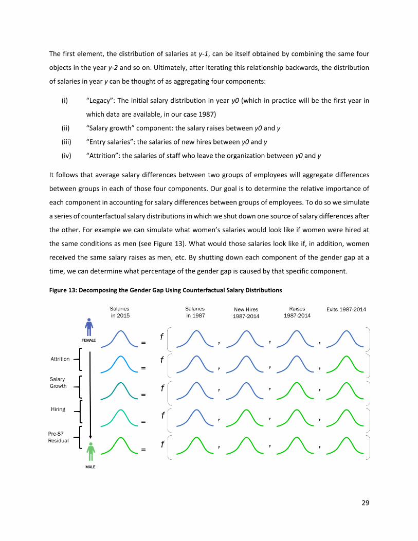
the same conditions as men (see Figure 13). What would those salaries look like if, in addition, women

received the same salary raises as men, etc. By shutting down each component of the gender gap at a

time, we can determine what percentage of the gender gap is caused by that specific component.

Figure 13: Decomposing the Gender Gap Using Counterfactual Salary Distributions

30

An important consideration in applying this decomposition concept to the WBG salary data is that

employees are hired at a specific grade. This suggests that our “entry salaries” component should be

subdivided into the grades at which men and women are hired, and the entry salaries they receive

conditional on their hiring grade. This leaves us with five components: attrition, salary growth, entry

salaries, grade composition of hires and legacy.

Appendix 2 describes in detail how the decomposition is implemented using simulations. In brief, the

procedure involves the following steps. First we estimate from our data simple parametric models for

each decomposition component, in each year and for each group of employee that we are concerned

with. For example, we estimate the probability of leaving the bank in 1995 for a Part 1 male employee

hired as a GF, as a function of his current salary. Next, taking as given the initial 1987 distribution of

salaries, we use the estimated models to simulate the salary raise that each employee receives in each

year, whether they leave the WBG in each year, as well as the salaries of new hires, all the way to 2015.

After verifying that the simulations for 2015 reproduce accurately the 2015 data, we can use the

simulation model to produce counterfactual salary distributions in which, for example, the parameters

governing the salary growth for women are replaced by the parameters governing salary growth for men.

The procedure described above decomposes the difference in salaries between two groups of employees

in a given year, which we have called the “aggregate gap”. However, the same method can also be adapted

to conduct an analysis by tenure. The object of interest in that case is salary gaps as they develop over the

employee's careers, which we call the “career gap”. To do so, the data are arranged by years of tenure

instead of by calendar year. Hiring salary, attrition, and salary growth processes are also estimated for

each year of tenure. The simulation algorithm starts by drawing a distribution of entry salaries and

proceeds to simulate salary growth and exits for each year of tenure.

This decomposition method has several strengths. First, the factors identified in the decomposition

correspond to well-defined Human Resources levers. Namely, the policies concerning raises and

promotions, the policies regarding new hires and the policies regarding retention of employees. An

important point regarding the interpretation of the results, is that this decomposition is not concerned

with determining why each of these policies have favored men over women or some nationalities over

others. For example, if male hires receive higher salaries than female hires, we do not attempt to separate

whether this is due to discrimination or to objective differences in qualifications among male and female

candidates. Instead, the type of statement that we can make is for example: “80 percent of salary

31

differences between men and women originate from differences in the salaries negotiated upon joining

the WBG.”

A second advantage of this method is that it accounts for the role of attrition, which, as documented

earlier, is sizeable. This is because the data allow us to observe employees who have left the Bank and

infer what current salaries would look like if they had stayed in the institution. Note that this is done at

the cost of the assumption that they would have received the same salaries on average as the employees

of the same group, entry grade and cohort who ended up staying and who had the same salary level as

them at the time of their departure. In addition, the decomposition can handle the pervasive non-

stationary or cohort-specific trends exhibited by salaries and employee composition in the data, as

documented in the earlier sections of this report.

The following sections describe the results of our decomposition of the aggregate gender gap, the

aggregate country part gap, the career gender gap and the career country part gap.

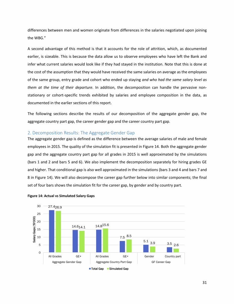
2. Decomposition Results: The Aggregate Gender Gap The aggregate gender gap is defined as the difference between the average salaries of male and female

employees in 2015. The quality of the simulation fit is presented in Figure 14. Both the aggregate gender

gap and the aggregate country part gap for all grades in 2015 is well approximated by the simulations

(bars 1 and 2 and bars 5 and 6). We also implement the decomposition separately for hiring grades GE

and higher. That conditional gap is also well approximated in the simulations (bars 3 and 4 and bars 7 and

8 in Figure 14). We will also decompose the career gap further below into similar components; the final

set of four bars shows the simulation fit for the career gap, by gender and by country part.

Figure 14: Actual vs Simulated Salary Gaps

27.4

14.6 14.8

7.55.1

3.5

26.9

14.115.6

8.5

3.92.6

0

5

10

15

20

25

30

All Grades GE+ All Grades GE+ Gender Country part

Aggregate Gender Gap Aggregate Country Part Gap GF Career Gap

Sa

lary

Ga

ps (

'$'0

00

)

Total Gap Simulated Gap

32

Figure 15 shows how the decomposition of the aggregate gender gap is obtained by the methodology

described in the previous section. Equating attrition probabilities across men and women closes 0.6

percent of the gap. Further equating salary growth closes an additional 5.4 percent and equating entry

salaries accounts for another 7.3 percent. These three factors explain together only 13.3 percent of the

gap. 76.2 percent of the gap corresponds to hiring grade composition effects whereby women are

disproportionately hired at lower grades. The remainder of the gap (10.5 percent) can be attributed to

differences between men and women hired before 1987 (the ``initial'' distribution).

For grades GE and higher, the decomposition factors are shown in Figure 15, right graph. The composition

of hires remains the most important factor to explain the gender pay gap. This is not surprising when one

considers, as we have noted in previous sections, that the WBG hired many more men than women at the

higher grades such as GG or GH throughout the period. Note that differential attrition has the effect of

bringing male and female salaries closer together, i.e. it contributes negatively to the gender gap.

Figure 15: Decomposition of the Aggregate Gender Gaps

3. Decomposition Results: The Aggregate Country Part Gap The results of the decomposition of the pay gaps between Part 1 and Part 2 employees are presented in

Figure 16. Equating attrition probabilities across Part 1 and Part 2 employees closes 14.5 percent of the

gap. Further equating salary growth closes an additional 6.2 percent and equating entry salaries accounts

for another 10.5 percent. These three factors explain together 31.2 percent of the gap. The bulk of the

0.6

-9.7

5.4 7.47.39.8

76.2 76.9

10.5

16.5

-20

-10

0

10

20

30

40

50

60

70

80

All staff (27.4k) GE+ staff (14.6k)

Co

ntr

ibu

tio

n t

o t

he

Ga

p (

%)

Attrition Salary Growth Entry Salary Grade Composition Pre-1987

33

gap (60.7 percent) again corresponds to the fact that Part 2 employees are on average hired at lower

grades. The remainder of the gap can be attributed to differences predating 1987. Within the GE+

category (Figure 16, right graph), the composition of hires again explains the majority (52 percent) of the

gap.

Figure 16: Decomposition of Aggregate Gaps by Country Grouping

4. Decomposition Results: The GF Career Gap We now decompose the pay gaps as they develop over the course of a career. We simulate the salaries

of employees hired between 1987 and 2001 onwards for 15 years. The choice of 15 years reflects a trade-

off between capturing career dynamics at higher grades, which necessitates a long span, and obtaining

results that are relevant to a large fraction of employees, rather than the small subgroup that accumulates

20 years of tenure at the WBG or more. As we discuss in section III.2, most hiring grades are not amenable

to this decomposition, either because the salary gaps are too small, or because there are not enough

individuals of each subgroup hired at that grade. We thus focus on GF hires, a group that includes large

enough gender-by-country part subsamples and exhibits sizeable pay gaps among them. Note that since

grade GF is one of the most common entry grades, we still cover 37.1 percent of all employees in grades

GE+ despite this restriction.

To examine the gender career gap, we first compare male Part 1 and female Part 1 employees hired at

the WBG headquarters at grade GF between 1987 and 2001. As seen in Figure 17, left graph, this gap is

mostly due to differences in salary growth (84.5 percent), while attrition, salary growth and entry salaries

14.5

7.96.2

10.710.512.5

60.7

52

8.1

16.9

0

10

20

30

40

50

60

70

All staff (14.8k) GE+ staff (7.5k)

Co

ntr

ibu

tio

n t

o t

he

Ga

p (

%)

Attrition Salary Growth Entry Salary Grade Composition Pre-1987

34

conditional on grade explain only 15.5 percent of it. A similar story emerges when comparing male Part

1 employees with male Part 2 employees. In this case (Figure 17, right graph), salary growth more than

explains the total gap (123 percent), and differential attrition works in the opposite direction.

Figure 17: Decomposition of the Career Gaps

5. Discussion of the Results The main insight from the decomposition exercise is that in terms of the aggregate gap, the historical and

continuing differences in entry grades are the major contributors. Career gaps arise sporadically across

grades and GF is the only entry grade with sufficient sample and sufficient salary gaps after 15 years for a

meaningful decomposition exercise. These results are at odds with the prior results of Filmer et al. (2005)

and with a prevailing view in the institution that there is considerable difference in the pay and promotion

by sex and nationality at the WBG.

We therefore conclude our analysis with a brief discussion of two further issues. First, we reconcile the

prior results of Filmer et al. (2005) with our findings. Second, we assess whether equity across subgroups

comes at the “cost” of rewarding performance. That is, if salary increases are arbitrary, there is little

reason for differences to arise across subgroups. Whether the WBG both rewards performance and limits

differences by sex and nationality or whether it limits differences by subgroups by limiting rewards to

performance is an important issue in its own right.

10.3

-34.6

84.5

123.1

5.211.5

0 00 0

-60

-40

-20

0

20

40

60

80

100

120

140

Male Part 1 vs. Female Part 1 (5.1k) Male Part 1 vs. Male Part 2 (3.5k)Co

ntr

ibu

tio

n t

o t

he

Ga

p (

%)

Attrition Salary Growth Entry Salary Grade Composition Pre-1987

35

To reconcile our results with Filmer et al. (2005), Table 3 replicates their gender gaps, noting that these

numbers do not account for differences in the entry grades of employees. We consider the 1997 cross-

section in our sample and apply the same sample restrictions, to the extent that we could identify them.

While our samples do not perfectly match, we obtain very similar gender and country part gaps, with large

differences in salaries in favor of Part 1 men and against Part 1 women and all Part 2 employees. We then

look at the subsample of staff hired after 1987, for whom we are able to identify the grade at which they

were hired. The pay gaps are a bit smaller (probably because they are from younger cohorts) but still large.

We then consider subgroups that are homogeneous with respect to their entry grade and these

differences become much smaller and sometimes disappear altogether. In other words, our results are

fully compatible with those of Filmer et al. (2005) and suggest again that differences in entry grades are a

key component of differences in salaries between subgroups at the WBG.

Table 3: Comparison to the Salary Gaps Obtained by Filmer Et Al. (2005)

Salary in 1997 Entry Salary Tenure in 1997 N

Filmer et al.

(2005), table 1

Male - Part I 100 100 11.9 1356

Male - Part II 95.3 91.4 12.5 857

Female - Part I 86.6 86.4 10.7 537

Female - Part II 82.5 80.6 11.2 250

Replication:

Employees hired at

GE+ grades

Male - Part I 100 N/A 11 1745

Male - Part II 94.3 N/A 11.6 1143

Female - Part I 84.1 N/A 10.6 752

Female - Part II 74.7 N/A 11.8 440

Employees hired

after 1987 at GE+

grades

Male - Part I 100 N/A 4.7 886

Male - Part II 92.5 N/A 5.3 516

Female - Part I 88.8 N/A 4.3 405

Female - Part II 80.6 N/A 4.4 200

Employees hired at

GF after 1987

Male - Part I 100 100 4.5 264

Male - Part II 100.6 98.3 5.2 209

Female - Part I 99.1 101.5 4.6 190

Female - Part II 96.3 94.2 4.3 112

Employees hired at

GG after 1987

Male - Part I 100 100 5 546

Male - Part II 97.6 94 5.4 254

Female - Part I 93.5 94.5 3.8 157

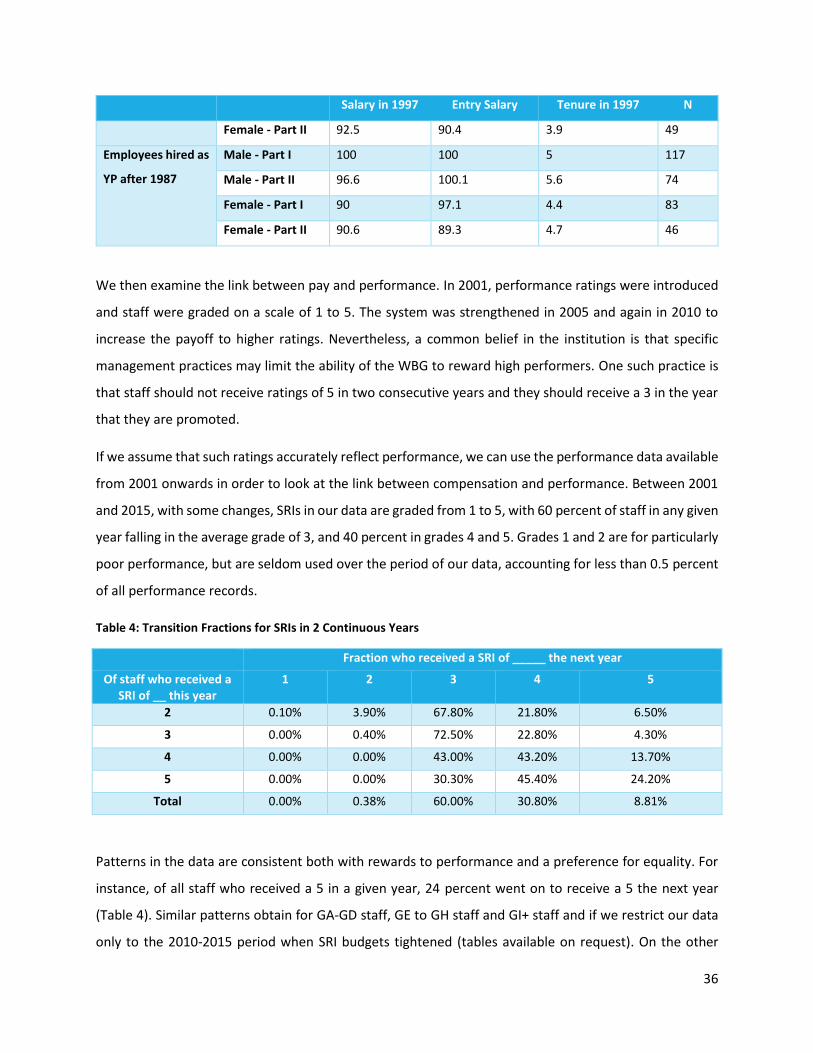
36

Salary in 1997 Entry Salary Tenure in 1997 N

Female - Part II 92.5 90.4 3.9 49

Employees hired as

YP after 1987

Male - Part I 100 100 5 117

Male - Part II 96.6 100.1 5.6 74

Female - Part I 90 97.1 4.4 83

Female - Part II 90.6 89.3 4.7 46

We then examine the link between pay and performance. In 2001, performance ratings were introduced

and staff were graded on a scale of 1 to 5. The system was strengthened in 2005 and again in 2010 to

increase the payoff to higher ratings. Nevertheless, a common belief in the institution is that specific

management practices may limit the ability of the WBG to reward high performers. One such practice is

that staff should not receive ratings of 5 in two consecutive years and they should receive a 3 in the year

that they are promoted.

If we assume that such ratings accurately reflect performance, we can use the performance data available

from 2001 onwards in order to look at the link between compensation and performance. Between 2001

and 2015, with some changes, SRIs in our data are graded from 1 to 5, with 60 percent of staff in any given

year falling in the average grade of 3, and 40 percent in grades 4 and 5. Grades 1 and 2 are for particularly

poor performance, but are seldom used over the period of our data, accounting for less than 0.5 percent

of all performance records.

Table 4: Transition Fractions for SRIs in 2 Continuous Years

Fraction who received a SRI of _____ the next year

Of staff who received a SRI of __ this year

1 2 3 4 5

2 0.10% 3.90% 67.80% 21.80% 6.50%

3 0.00% 0.40% 72.50% 22.80% 4.30%

4 0.00% 0.00% 43.00% 43.20% 13.70%

5 0.00% 0.00% 30.30% 45.40% 24.20%

Total 0.00% 0.38% 60.00% 30.80% 8.81%

Patterns in the data are consistent both with rewards to performance and a preference for equality. For

instance, of all staff who received a 5 in a given year, 24 percent went on to receive a 5 the next year

(Table 4). Similar patterns obtain for GA-GD staff, GE to GH staff and GI+ staff and if we restrict our data

only to the 2010-2015 period when SRI budgets tightened (tables available on request). On the other

37

hand, as a staff member’s salary increases within the same grade, their subsequent salary increase slows

down. For those who are above the “midpoint” of the salary band at their grade-level, high performance

yields marked compensation increases only if the staff member is promoted. For instance, in our data

there are two variables that show the salary raise in a given year for an employee—the raise that an

employee would receive based on his/her SRI alone and the actual raise that takes into account the

relative compensation of the staff at his/her grade level. In a regression context, the “midpoint” penalty

implies that, after conditioning on grade, an increase in the SRI implies a 1.9 percentage point salary

increase, but there is a 0.6 percentage point penalty for every $10,000 increase in the initial salary.

Similarly, large policies appear not to be reflected in performance ratings. For instance, in 2010, a

significant change was introduced, whereby new hires would be given 3 year contracts with renewal based

on performance. This could have incentivized performance, but we do not see higher SRIs on average for

staff hired in 2011 and 2012. The SRI obtained over the first three years at the WBG remains the same for

staff hired in 2008 (SRI=3.31), 2009 (SRI=3.31), 2010 (SRI=3.34), 2011 (SRI=3.32) and 2012 (SRI=3.25).

An alternate way to assess performance rewards is to examine the diversity in performance of cohorts

over time. Take for instance the 2005-2015 period, where the SRI system has been in place for 10 years

and consider the salary structures of those who were hired between 2000 and 2005. The worst 10 percent

of performers among staff who entered as GF between 2000 and 2005 in a balanced panel over this period

has an average SRI of 3.22; the best 10 percent of performers has an average SRI of 4.30.

These differences in average SRIs led to large variation in pay (Table 5). By 2015, the best 10 percent saw

their salary increase by 83% against 26% for the worst 10 percent. Nevertheless, these rewards are not

seen as clearly through the entire distribution of performance. There is a clear penalty for staff in the

lowest decile, and to a lesser extent, to deciles 2, 3 and 4, and a clear reward for those in the top decile

with muted differentiation among staff in deciles 5 through 9. A hypothesis consistent with these data is

that most of the difference in salaries is due to promotions rather than annual salary raises within the

same grade. The fraction of employees promoted to GH or more within 10 years is lower than 17 percent

for the first 4 deciles, between 30 and 40 percent for deciles 5 through 9, while 5 percent of employees in

the top decile are already at grade GI by that time and 50 percent are GH.

38

Table 5: Salaries and Promotions by Mean Performance Ratings Aggregated over 10 Years (staff hired at GF in 2000-2005)

Bottom decile

2nd 3rd 4th Middle decile

6th 7th 8th 9th Top decile

Start Salary

100 98 99 99 98 99 98 98 101 99

10 year salary

growth

26% 38% 45% 49% 55% 58% 65% 68% 69% 83%

%GG after 10

yrs

60 74 79 71 59 63 61 58 63 45

%GH after 10

yrs

1 4 12 16 26 29 33 38 37 53

%GI after 10

yrs

0 0 0 0 0 0 1 0 0 3

V. Conclusion We have analyzed salary differences at the WBG between 1987 and 2015 in terms of differences by sex

and by nationality. Our analysis begins with the idea that aggregate and career gaps can be examined as

an interplay between composition and compensation effects and our decomposition results suggest that

composition effects play the major role in explaining the aggregate gap in 2015. The career gap in

general—and especially among GE+ staff where sample sizes are sufficient for meaningful comparisons—

tends to be small at the WBG with entry salaries, salary growth and exits contributing in different

proportions depending on the grade at which the employee was originally hired.

As a research paper, the objective is to establish basic facts that can inform discussion and debate at the

WBG. One general theme that emerges from this line of work is that pay distributions today are linked in

complex ways to historical hiring and compensation patterns. Conversely, policies today will have long-

run effects that need to be carefully considered. For instance, attempts to increase the number of women

at the GH level through greater hiring at the GF level and promotions would have to account for the fact

that men tend to leave the institution at a faster rate than women and that overall exits are highly cyclical.

Consequently, boosting hiring at the bottom of an exit-cycle can have very different long-term effects

relative to additional hiring at the peak of the cycle. Similarly, one-time salary raises to staff who are below

a benchmark would have to be evaluated both in terms of their effects on the balance between pay and

performance as well as the design of the compensation system.

39

Two specific issues stand out for further attention. First, compositional differences continue to affect the

distribution of staff at the WBG. We do not know whether these differences emerge at the point of hiring

(equally qualified men and women have applied, but men are chosen more often) or at the point of job

applications (fewer qualified women apply relative to men). Data on job applicants are currently not

available in the HR system and further, even for those who are successfully hired into the WBG, data on

personal characteristics are incomplete. For instance, education levels measured as the highest degree is

missing for 55 percent of staff in the data. If compositional differences arise at the application stage, a

very different kind of policy would be required (such as an outreach program) relative to compositional

differences that arise at the hiring stage given an equal application pool across all subgroups.

Second, exit rates from the institution are such that 50% of staff leave within 7-9 years. Little is known

about why staff leave the institution and what jobs they receive outside the WBG. Further, managers may

have flexibility to negotiate, but new tools may need to be leveraged better to retain staff who plan to

leave. Our analysis revealed that those who leave and those who stay look very similar on their

performance at the WBG prior to their exit. Therefore, the institution loses both high and low performing

staff whenever the number of exits rises. Appropriate actions that can be taken to retain high-performing

staff—especially women and Part 2 staff—may be a useful new area for policy or simply be an area that

needs to be better managed within the institution.

40

References Blau, Francine D., and Lawrence M. Kahn. 2016. “The Gender Wage Gap: Extent, Trends, and Explanations.” IZA Working Paper 9656, January Deon Filmer, Elizabeth King, Dominique van de Walle. 2005. "Testing for pay and promotion bias in an international organization", International Journal of Manpower, Vol. 26 Issue 5, pp.404 – 420

Gobillon, Laurent, Marion Leturcq, Dominique Meurs and Sebastien Roux. 2014. Elite Institutions, fields

of study and the gender wage gap: case study of a large firm. File downloaded on March 13, 2017 from

http://lagv2015.idep-fr.org/submission/index.php/LAGV2015/LAGV14/paper/viewFile/1653/376

Juhn, Chinhui and Kristin McCue. 2017. Specialization Then and Now: Marriage, Children, and the

Gender Earnings Gap across Cohorts. Journal of Economic Perspectives. Vol. 31 (1): pp. 183-204

Keane, Michael P., and Kenneth I. Wolpin. "The role of labor and marriage markets, preference

heterogeneity, and the welfare system in the life cycle decisions of black, hispanic, and white women."

International Economic Review 51.3 (2010): 851-892.

Takao, Kato, Daiji Kawaguchi and Hideo Owan. 2013. Dynamics of the Gender Gap in the Workplace: An

econometric case study of a large Japanese firm. The Research Institute of Economy, Trade and Industry

Discussion Paper Series 13-E-038.

The LSE Equity, Diversity and Inclusion Taskforce. 2016. The Gender and Ethnicity Earnings Gap at LSE.

The World Bank. 2012. World Development Report: Gender Equality and Development.

41

Appendix Figures and Tables

Appendix Figure 1: New Hires around the 1998 Reform

Notes: The figure shows the number of staff hired in each year in different grade categories. The figure highlights the significant changes around 1998 reform with a sharp decline in ungraded staff and a corresponding spike in GE+ and GA-GD hires.

0

200

400

600

800

1000

1200

No

. o

f P

eo

ple

Hir

ed

GE+ Staff GA-GD Staff Ungraded Staff

42

Appendix Figure 2: Real Salary Growth of New Entrants by Grade and Year

Notes: The figures shows the real salary growth of new entrants at each grade. Salaries are normalized to a base of 100 for each grade in 1988 and deflated using the U.S. Consumer Price Index.

100

110

120

130

140

150

160

1988-1990 1991-1995 1996-2000 2001-2005 2006-2010 2011-2015

Ave

rage

Re

al S

ala

ry (

19

87

=1

00

)

GA

GB

GC

GD

GE

GF

GG

GH

GI

GJ

GK

43

Appendix Table 1: Number of Staff by 2-digit Nationality Code

Part 1 Part 1/Part 2 Part 2

AE 1 ES 340 AF 28 DO 40 LC 5 SD 28

AT 142 EE 6 AG 4 DZ 59 LK 214 SG 73

AU 497 PT 70 AL 28 EC 93 LR 37 SI 6

BE 258 LV 8 AM 38 EG 164 LS 5 SK 27

CA 897 LT 14 AO 2 ER 5 LY 5 SL 65

CH 140 GR 97 AR 359 ET 185 MA 81 SN 135

DE 785 AZ 16 FJ 2 MD 31 SO 13

DK 194 BA 20 GA 10 MG 38 SR 1

FI 141 BB 22 GD 10 MK 15 ST 1

FR 1,293 BD 129 GE 32 ML 37 SV 48

GB 1,513 BF 30 GH 185 MM 17 SY 18

IE 201 BG 85 GM 16 MN 21 SZ 3

IS 13 BH 2 GN 21 MO 1 TD 10

IT 503 BI 18 GT 44 MR 16 TG 23

JP 722 BJ 38 GW 1 MT 4 TH 118

KW 22 BM 3 GY 69 MU 100 TJ 15

LU 7 BN 1 GZ 5 MW 31 TM 2

NL 359 BO 142 HK 4 MX 278 TN 63

NO 150 BR 435 HN 41 MY 136 TO 1

NZ 123 BS 8 HR 17 MZ 13 TR 269

RU 250 BT 10 HT 84 NA 4 TT 115

SE 230 BW 10 HU 50 NE 15 TW 1

US 9,062 BY 18 ID 107 NG 179 TZ 51

XB 7 BZ 7 IL 81 NI 49 UA 91

ZA 146 CF 4 IN 1875 NP 83 UG 109

CG 18 IQ 11 OM 1 UY 76

CI 104 IR 138 PA 28 UZ 41

CL 220 JM 154 PE 386 VC 1

CM 104 JO 63 PG 2 VE 95

CN 649 KE 215 PH 928 VN 108

CO 382 KG 30 PK 335 WS 1

CR 58 KH 8 PL 78 XK 11

CS 3 KM 2 PY 24 YF 56

CU 18 KN 3 RO 71 YU 1

CV 3 KR 290 RW 17 ZM 50

CY 24 KZ 35 RY 10 ZR 16

CZ 32 LA 7 SA 56 ZW 77

DJ 4 LB 165 SC 1

44

Appendix Table 2a: Relative salaries of employees who leave the WBG vs those who remain (Base: GA-GD non-attritors with 5 years of experience)

Hiring Grade and Years of Tenure Attrition Status

Non-Attritors Attritors

GA-GD

5 100 103

10 119 123

15 139 142

GE

5 164 162

10 208 201

15 250 256

GF

5 216 217

10 270 268

15 326 324

GG

5 284 289

10 330 334

15 337 382

Notes: The table shows the relative salaries of staff who exit the WBG and those who choose to remain for different entry grades and different tenures. The salaries are normalized with the GA-GD staff who left the WBG within 5 years chosen as the base of 100.

45

Appendix Table 2b: Mean Performance Rating of employees who leave the WBG vs. those who remain

Hiring Grade and Years of Tenure Attrition Status

Non-Attritors Attritors

GA-GD

5 3.4 3.3

10 3.6 3.5

15 3.6 3.5

GE

5 3.3 3.2

10 3.6 3.5

15 3.6 3.6

GF

5 3.3 3.2

10 3.6 3.5

15 3.7 3.6

GG

5 3.3 3.2

10 3.6 3.5

15 3.7 3.6

Notes: The table shows the mean performance rating of staff who exit the WBG and those who choose to remain for different entry grades and different tenures. For instance, the average performance rating of all staff who entered as GF but left the WBG (“attritors”) after 5 years was 3.3 compared to 3.2 for those who chose to remain at 5 years.

Technical Appendix World Bank Group HR Longitudinal Database

1

Appendix I Data Description

World Bank Group HR Longitudinal (Panel) Database

Technical Appendix World Bank Group HR Longitudinal Database

2

Bibliographic Citation Publications based on WBG Human Resource Development (WBG HRD) data collection should acknowledge those sources by means of bibliographic citations.

World Bank Group HRDDI/DEC. WORLD BANK GROUP HUMAN RESOURCE PANEL DATA 1987-2015 [COMPUTER FILE]. Washington DC: World Bank Group, Human Resources Development Diversity and Inclusion Office, 2015.

Request for Information on use of WBG HR Resources A request for using this data must be submitted to the manager of the WBG Human Resources Department of Diversity and Inclusion (HRDDI) and the WBG Vice-President of Human Resources (HRDVP). Data Disclaimer The data in this dataset are property of the World Bank Group (WBG) and strictly confidential. These data are not to be seen, distributed or used by any party without the explicit permission of the manager of the WBG Human Resources Diversity & Inclusion Office (HRDDI) and the WBG Vice-President of Human Resources (HRDVP). The original collector of the data, WBG HRDDI, bears no responsibility for uses of this collection or for interpretations or inferences based upon such uses. Data Collection Description SUMMARY: The purpose of collecting long-term human resource (HR) data is to provide deeper insight on career development, including pay and performance, of staff in the World Bank Group. Particular emphasis is placed on exploring how different dimensions of diversity such as gender relate to pay and performance. Using data sources such as PeopleSoft and Business Intelligence, data were provided by different HR teams such as the performance & compensation team. The Development Research Group (DEC) provided the data and calculations for CPI and PPP adjustments of salaries. Most data came from PeopleSoft. Variables include the staff’s unique personnel identifier (UPI), the year in which the snapshot was taken, indicators of employment status, appointment types, duty location countries and cities, salaries, units, age, performance ratings, salary increases, departments and diversity dimensions.

EXTENT OF COLLECTION: 1 data file (.dta format) Structure: Rectangular, panel data Cases: 349448 (upi-years) Variables: 65 Records per case: 1

Technical Appendix World Bank Group HR Longitudinal Database

3

Technical Appendix

World Bank Group Human Resources (HR) Longitudinal (Panel) Database

I. Presentation We describe the methodology for coding and building the “WBG Human Resources Longitudinal Database”, which is a panel data set on WBG human resource data from 1987-2015. We first present the overall structure of the database and describe the different data warehouses from which it was constructed; second, we delineate the general rules and criteria we used for coding and merging; then we present a selection of important variables, their original and raw coding and definitions in a short codebook of the variables. We subsequently provide a more extensive explanation of this host of important variables, the changes and standardizations we applied to them, as well as describing institutional changes that took place over the course of the years covered.

II. Overall structure of the database and sources Structure: This section presents the overall structure of the WBG HR Longitudinal Database and describes the different data sources used.

The dataset is structured in a panel format, with each fiscal year representing one part of the panel. The overall design is modular. There are two skeletal variables that make up the backbone of the dataset: the universal personnel identifier (UPI) and the fiscal year (FY). All the other variables were then added to these UPI-years.

o Universal personnel identifiers never change for an individual, even if the staff member has several breaks in service of employment at the WBG.

o The dataset runs from fiscal years 1987 to 2015. Each yearly snapshot is taken as per June 30th of that year, which is the end of a fiscal year. The 1988 snapshot, for example, is as of 6/30/1988.

Data Sources: At this time, the WBG does not have a unified data warehouse that contains all human resource data. The HR longitudinal database is therefore built from multiple sources:

PeopleSoft/Business Intelligence (BI): The most important source of data is PeopleSoft, which contains elements such as WBG staff’s universal personnel identified (UPI); salaries (in net terms); salary administration plan (what plan they are on); personal backgrounds (e.g. gender, age); professional situation (e.g. professional grade); location (e.g. HQ or country-office based); role and movements within the organization (e.g. promotions and lateral moves); and compensation and benefits (e.g. salaries). Whether or not an HR analyst has access to compensation and benefits data depends on the level of access. The PeopleSoft data can be accessed through SAP Business Intelligence.

o In general, the data are organized into stock and flow data. The stock data are updated daily. Daily snapshots are not saved, however. At the end of every month, a snapshot of the personnel records is frozen in time and saved for future use. The flow data can be accessed through a custom timeframe, including the first and last day of flow data.

Technical Appendix World Bank Group HR Longitudinal Database

4

o Through BI, one can only go back as far as fiscal year (FY) 2000, but a custom request to the HR Reports department allows one to go back further than the year 2000. This meant that construction of the database entailed merging pre and post 2000 data.

Talent Management: The WBGs Talent Management Unit is responsible for keeping records of talent development, including the numbers of identified ‘top talents’ at different grade levels. This data also includes observations on the yearly performance rating, also known as SRIs, which co-determine salary increases.

Family Data: Data on the family situation of staff is housed under a separate roof as well. This includes variables on the number of members in the household, as well as the marital status of the staff member.

Merging: Data from these different sources were merged using the skeletal variables mentioned above (UPI and Fiscal Years). Deleted data: After the merging process, the following data were deleted.

Observations that had year marked as 0.

1165 observations with a missing salary. This had several reasons: o Performance rankings are, on a different time schedule resulting in some employees

who received a performance ranking, but by the time we see them in the dataset, have left the WBG. Or, conversely, they were given a `fictional’ SRI for a performance year in which they did not work because they joined in that year. This is due to the retroactive character of the performance ratings. The merge from the performance data created such observations, which cannot be linked to the larger dataset.

o Some missing data are because we integrated an indicator for whether the staff was a Young Professional from another dataset. The WBG HR systems, however, mark somebody who was once a YP as always a YP. Employees who remain after retirement or exit as short term or part-time consultants will be merged in with their UPI but will not have wage data as they are no longer considered staff.

o Third, there are staff who go on secondments where they are no longer paid by the WBG, or are on leave without pay, when their salaries also disappear. This happens for several personnel members for some individual or groups of years over their employment spells at the Bank.

Finally, there are those whose salaries are marked as 0. These are people on special assignment, therefore these are also graded Unclassified UCs, and they do not receive any salary that year.

III. General rules and criteria

In building, standardizing and cleaning the dataset, we used several different general rules and criteria.

1. General Definitions: In general, we aimed to use and thereby maintain the integrity of the WBG internal definitions.

2. Employee Selection The WBG has several different types of employees. The most important broad distinction is between staff members and consultants. Within these two large categories, several sub-categories existed. In addition, these sub-categories have shifted significantly over time. A third but small category, often captured in the systems as staff members who are unclassified, are executive directors and their advisors.

a. In general, database excludes short-term consultants since little data is available on them, and they are not fulltime staff members. However, so-called long-term

Technical Appendix World Bank Group HR Longitudinal Database

5

consultants (LTCs) as well as its later form – Extended Term Consultants (ETCs) – are included in the database, since these contract types represent full-time consultancy positions with the WBG.

b. Executive Directors and their Advisors are included in the database, but excluded from the analysis since they are not paid by the WBG but by the governments they represent.

3. Variable names and labels: The WBG HR systems variable names and labels were changed to increase readability. For example, the label gradecurr was changed to “original unstandardized WBG professional grade” or the label `eod’ was replaced with “entry-of-duty”.

4. String to numeric: Several numeric variables were marked as string variables by default. This included, for example, the yearly snapshot data. We changed these string variables into numeric variables where appropriate to make it easier to work with the data.

5. Binary variables: We consistently recoded binary variables into zeros and ones. 6. Variable Standardization and Modernizations: WBG HR systems have changed multiple times

over the span of the dataset (1987-2015). As such, data definitions have also changed for multiple variables. Where possible, we recoded variables in such a way that the definitions reflect the current protocols

IV. Overview of selected important variables This section presents a short overview of a selection of variables that are particularly important, difficult to understand or work with, or needed conversions or fixes. The variables are divided into six categories.

Variable Name (label) Variable Values or explanation

1. Backbone variables

Upianonymous Anonymous UPIs Used for merging with data from departments that should not have access to full HR data

upi (UPI)

Unique identifier for staff

year (Year)

Fiscal year – the data recorded per the 30th of June every year, with the exception of 2015.

1987 1988 …… 2015

2. Salary Variables

salarycurr Salary in local currency for that upi-year. This is a net salary, irrespective of whether the staff is required to pay taxes.

E.g. 500000 will be 50.000 dollars if it is a U.S. salary administration plan or 100.000 on a Turkish salary plan will reflect a salary of 100.000 Turkish Liras.

Net/Gross

salarycurrency

Salaryadminplan (Salary What salary administration plan Examples

Technical Appendix World Bank Group HR Longitudinal Database

6

Admin Plan) the member is on, for example “US” refers to the United States salary plan. This thus also indicates the currency the staff is paid in

KH Cambodia

CN China

HK Hong Kong SAR, China

ID Indonesia

KI Kiribati

KR Korea, Rep.

LA Lao PDR

MY Malaysia

MN Mongolia

MM Myanmar

PG Papua New Guinea

PH Philippines

TH Thailand

TP Timor-Leste

TO Tonga

VN Vietnam ………

Global Payroll Group (Global payroll Group)

Indicates in what currency the staff member is paid out. This variable is not as complete as the salaryadminplan variable.

Examples include AFGUSD, which means Afghanistan United States Dollars, TURTRY indicates Turkish Liras.

Paygroup (Pay Group)

Indicates in what pay group the staff member falls, with aggregated codes for those under the United States Plan. It has less missing values than the Global Payroll Group variable.

Examples in AFUSD, which means Afghanistan U.S. Dollars, SM1 means United States salary plan.

3. Variables on Professional Background

gradecurr (Grade(Curr)) Current grade of the staff. The grade structure has changed significantly over the time the panel data covers

e.g. ETC1, GA, GK, N, M, UC

orgalpha (Org (Alpha)) The organization the staff member is a part of, with organization referring to one of the institutions that make up the WBG together

“GEF” – Global Environmental Facility IBRD – International Bank for Reconstruction and Development IFC – International Finance Corporation MIGA – Multilateral Investment Guarantee Agency

eod (EOD)

The entry-of-duty date of the staff

Example: 07/31/1977

Technical Appendix World Bank Group HR Longitudinal Database

7

apptype (Appt Type) The type of appointment the staff member has, noted in a 3 to 5 letter code.

e.g. EDAT – ED Alternative, EDIR – Executive Director, HREG – HQ Regular

appttypename (Appt Type Name)

What type of appointment the staff member has, for example HQ Regular. More detailed than the 5-letter code.

e.g. ED Advisor, Extended Term Consultant, HQ Long Term Consultant, HQ Regular, Part Time Regular…

Pmucurr

Management unit that the staff is a member of for that year. For example, HRD refers to Human Resource Development. These codes have changed over time, and thus may be linked only to UPIs in certain years, and then disappear.

Examples (for full, see codebook): ACO – Appeals Committee AFR – Africa ASI – Asia VPU AST – Asia Regions Technical Department BOG – Board of Governors BPS – Budget, Performance Review and Strategic Planning CCG – Climate Change Group Vice Presidency

departmentname (Depart Name)

The name of the department, long code

Examples: ACO, AFC13-HIS, AFCMUS-HIS

Divisioncurr (Division (Curr))

The current division that the staff is a member of, with a mix of codes and full name descriptions

Examples: WBIGA, South Asia Country Dept III, AFTP1

divisionnamecurr (Division Name (Curr))

The current division that the staff is a member of, full name

Examples: World Bank Office: Guatemala City, WBG Treasury & Portfolio, Public-Private Partnerships

divstream (Div Stream)

Division stream the staff is a member of

Examples: international trade division, Pop & Human Resources Opr Div, Regional mission: Nairoibi

highestdegree (Highest Degree)

Denotes the highest degree of the staff member in a two or three-letter code

e.g. BL and BAC = Bachelor

highestdegreename (Highest Degree Name)

Denotes the field of the highest degree

Examples include Ph.D. Economics, Urban & Regional Planning, Water Resource Management

4. Variables on Personal Background

gender (Gender)

Indicates the gender of the staff member

F – Female M – Male

nationality (Nationality) Indicates the nationality of the staff member, both two-letter

Examples include AT and Austrian, even though both mean Austrian.

Technical Appendix World Bank Group HR Longitudinal Database

8

codes and full nationalities

Countrypart (Country Part)

Indicates which so-called country part the staff’s primary nationality corresponds with—either Part 1 or Part 2.

1 – Part I Country 2 – Part II Country

personalssacr (Personal.SSA/CR)

Indicates whether the staff is from Sub-Saharan Africa or from the Caribbean

CAR FSU ISC NOG SSA XCR

marital_descr (MARITAL_DESCR)

Description of the marital status of the staff member.

Divorced Head of Household Married Not Married Partnered Separated Unknown Widowed

5. Merge Variables

mergeFamily Leftover from matching family data into the dataset, and shows which staff members had family data

Master only (1) – UPI matched with no family data Matched (3) – matched on UPI

mergeExternalPayObs Leftover from matching individuals who were missing due to external service with pay

Master only (1) – Data was already in the dataset Matched (3) – additional data for those with external service included

mergeFamilyUpdate Indicates how the family data was added for those on external service with pay

Master only (1) Missing updated (4) – updated the family data for the external service with pay staff

6. Inflation and Purchasing Power Variables

Contcode 3 digits country code Example: USA – United States of America

cd Combination of countrycode and year

Example: Per2014 is Peru 2014

Ppp2005 Purchasing Power Parity Exchange rate 2005, expressed in United States dollars

Xchange05 Official exchange rate in 2005 with the 2005 U.S. dollar

Cpi Consumer price index

Cpi2005 Consumer price index 2005. The price index in 2005, this is the

Technical Appendix World Bank Group HR Longitudinal Database

9

baseline to which all other CPIs can be compared.

Cpi_rate A ratio of cpi2005/cpi. In other words, this is a comparison of each CPI (one for each country per year) with the CPI2005.

Salaryppp2005 Salary in 2005 PPP USD

V. Selected variables, definitions, fixes and conversions 5.1 Backbone variables UPI & Year The UPI & year are the two variables that form the primary keys for the panel dataset. They uniquely identify the staff member as well as the fiscal year in which we observe them. 5.2 Salary Variables Salary Salary is the salary in the system during the snapshot. It does not reflect the actual previous year’s salary, but the salary in the system at the point of measurement. Salary is always noted as a net salary in the system. International hires, who do not have a U.S. citizenship nor a green card, do not pay taxes over their WBG income. U.S. nationals do, but their salaries are recorded as net salaries in the system, to make them comparable to the salaries of international hires.

U.S. nationals receive a tax reimbursement through a separate system, to compensate them for the differential. After the reimbursement, the salary is not always completely identical to what an international hire would have earned, but it approximates it closely.

Salary increases derive from three sources: overall salary increases, performance-based increases and promotion-based increases.

A promotion to a higher professional grade is associated with the highest salary increase, since a staff member moves into a higher salary bracket.

Increases without promotions follow a different logic. These stem from increases based on performance as well as a non-performance based, broader salary increases for staff. Therefore, salary at t does not equate the salary at t-1 plus the increase associated with a particular performance rating. There is an additional part of the increase which takes place independently from performance.

In addition, the salary increase system is set-up such that those at a lower end of the spectrum receive higher increases than those at a higher end of the spectrum. Or, within a professional particular grade, individuals who are at a lower part of the salary scale associated with that grade receive higher relative increases than those who are at a higher end of the salary distribution.

Since the 1990s, the WBG compensation and benefits team have started conducting a yearly analysis to identify salary outliers and rectify them. Using regression analysis, the team looks throughout the WBG to look at individuals who earn 10% or more below the salary they can be

Technical Appendix World Bank Group HR Longitudinal Database

10

expected to have. If an outlier is identified, the manager of that unit will then be tasked with giving them a one-time large increase to rectify this. Outliers receiving over 10% more than what can be expected are not corrected.

On rare occasions, individuals experience a decrease in their nominal salary. This can happen if somebody decides to accept a demotion or salary decrease instead of losing their position. Over the span of the dataset, there are 34 observations where this is the case.

Salary currency

A majority of WBG staff are paid in U.S. dollars, but there are also a large number of observations who are paid in local currencies.

In general, staff who are based in the Washington DC Headquarters, are paid in U.S. dollars. Local staff can either be paid in U.S. dollars or in their local currency. Generally, international hires working in country offices are paid in U.S. dollars whereas locally-hired staff are paid in the local currency, with some exceptions.

Paygroup Paygroup and globalpayrollgroup are the exact same thing, but the globalpayrollgroup replaced the paygroup variable in FY14. It represents a combination of the salaryadminplan and the salary currency, but is not a very strong and complete variable. Salary Administration Plan The salary administration plan reflects the system a staff is mapped to, but not necessarily the currency they are paid in. In other words, the salaryadminplan does not necessarily equate the currency of that salaryadminplan. For example, staff in Russia might be on the Russian (‘RU’) salaryadminplan. This does not tell us whether they are paid in rubles or in dollars at a given time t. To derive this, one has to look at the salary currency indicator. The standard WBG two-letter country codes were used to standardize the salary administration plan and create consistency across the variables. 5.3 Variables on professional background Grades The WBG has changed the way in which it marks its professional grades over time. The current system grades employees from GA to GD for administrative and client services (ACS) staff. GE tends to refer to analysts, but is a somewhat heterogeneous category. GF to GG refers to professional technical staff. GH can refer to technical staff or managers. GI refers to directors, GJ to and GK to vice presidents and senior management and GL is the President of the WBG.

Over the course of the time covered by the dataset, there were two large changes. The original system ranged from A to P. However, a large proportion of staff were not given a particular grade at this time (see below).

After this point, there was a system in which the grades ranged in numbers from 1 to 31. Grades 1-10 described support staff such as cooks and drivers. Grades 10 to 31 to professional grades, with 10 to 17 (GA-GD) referring to different levels of administrative staff, and grades 18 and up to professional levels (GE+).

In 1999 the system changed to its current set of broad banding.

Throughout the years, there have also been two unclassified categories which are heterogeneous containers—UC and UA. Before the system of broad-banding, the UC category

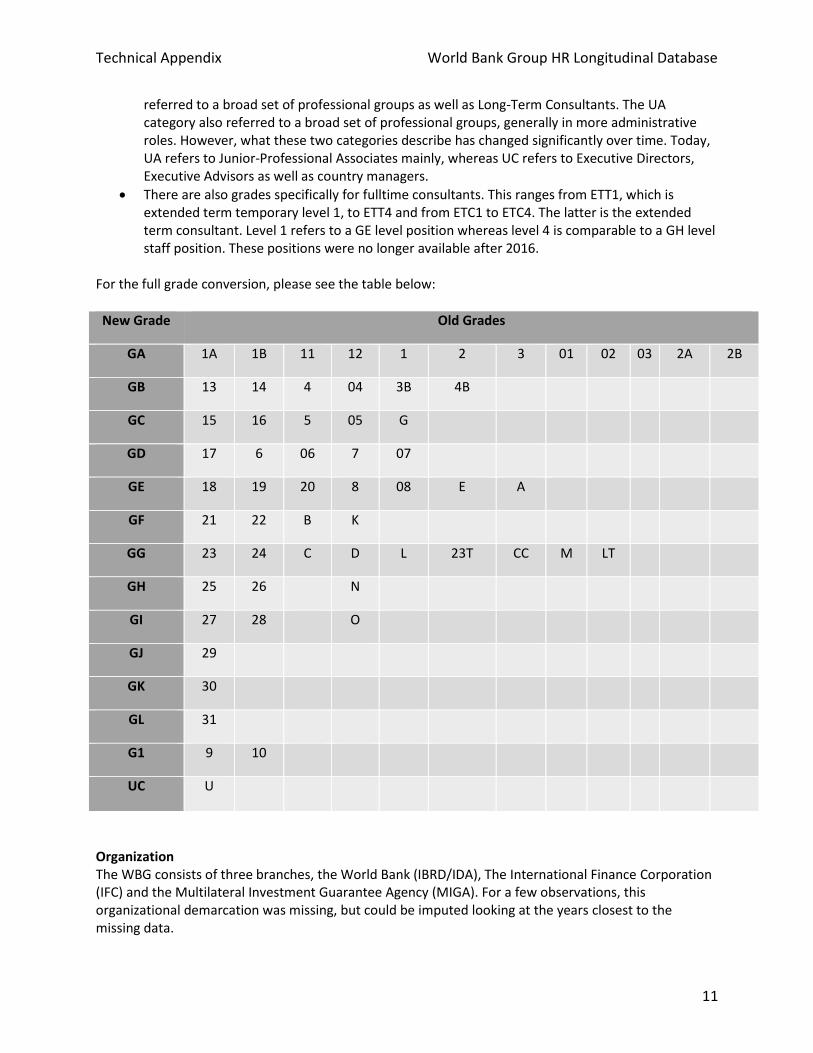
Technical Appendix World Bank Group HR Longitudinal Database

11

referred to a broad set of professional groups as well as Long-Term Consultants. The UA category also referred to a broad set of professional groups, generally in more administrative roles. However, what these two categories describe has changed significantly over time. Today, UA refers to Junior-Professional Associates mainly, whereas UC refers to Executive Directors, Executive Advisors as well as country managers.

There are also grades specifically for fulltime consultants. This ranges from ETT1, which is extended term temporary level 1, to ETT4 and from ETC1 to ETC4. The latter is the extended term consultant. Level 1 refers to a GE level position whereas level 4 is comparable to a GH level staff position. These positions were no longer available after 2016.

For the full grade conversion, please see the table below:

New Grade Old Grades

GA 1A 1B 11 12 1 2 3 01 02 03 2A 2B

GB 13 14 4 04 3B 4B

GC 15 16 5 05 G

GD 17 6 06 7 07

GE 18 19 20 8 08 E A

GF 21 22 B K

GG 23 24 C D L 23T CC M LT

GH 25 26 N

GI 27 28 O

GJ 29

GK 30

GL 31

G1 9 10

UC U

Organization The WBG consists of three branches, the World Bank (IBRD/IDA), The International Finance Corporation (IFC) and the Multilateral Investment Guarantee Agency (MIGA). For a few observations, this organizational demarcation was missing, but could be imputed looking at the years closest to the missing data.

Technical Appendix World Bank Group HR Longitudinal Database

12

Entry of Duty The entry of duty variable (EOD) is problematic, as individual employees can be given several EODs in different observation-years. This is primarily driven by the fact that the way the WBG recorded the EOD changed, reflecting therefore system-imposed changes rather than real changes. This is particularly noticeable from the year 1999 to 2000, when WBG HR Systems changed to record the most recent EOD rather than the first EOD. In other words, an individual employee who enters the WBG in 1973, left, and came back in 1976 will have an EOD of 1973 in each of the recorded years until 2000. In the observation-years post 2000, the EOD will read 1976. This was not fixed in the database, but is important to take into consideration when conducting analysis on the data. To provide an example: Person A starts working from 1983 to 1986 and then took a break from 1986 till 1990, before rejoining the WBG. We start observing this person in 1990 in our data. The EOD is WRONG for the years 1990 to 2000, as it should have been 1990 throughout, but it was only reset to 1986 in 2000 when they changed the logic of the recording. Country Codes: The WBG has two-letter country codes. This is a standardized matrix used for different country indicators, for example to show the salary administration plan, or to show the duty country of a staff member. E.g. the code for the Netherlands is “NL”. Appointment Type Appointment type reflects the type of contract a staff member is on. For example, a staff member can be on a multi-year or open-ended contract. The way in which appointment type was recorded changed over time. These different definitions were standardized to reflect the current (as of 2015) WBG appointment type definitions. See the table below for the standardizations:

Appointment Type Standardized Unstandardized

HQ Regular HQ Regular or Open-Ended Staff

Term Staff HQ Fixed Term or Term Staff

Local Staff Regular Appointment Local Regular

Local Staff Term Local Fixed Term

A2.01 The types of appointments to the staff of the WBG are specified below:

a. Regular Appointment is a full-time appointment of indefinite duration made before July 1, 1998.

b. Local Staff Regular Appointment is a full-time appointment of indefinite duration, made before July 1, 1998, of a person recruited to serve at a WBG country office.

c. Open-Ended Appointment is an appointment of indefinite duration made after June 30, 1998. d. Term Appointment is an appointment for a specified duration of a minimum of one year and a

maximum of five years per appointment except: i. a staff member who joins the WBG under the Junior

Professional Associate Program can be appointed for a maximum of two years, and;

Technical Appendix World Bank Group HR Longitudinal Database

13

ii. for a staff member appointed to an Administrative Client Support position in the Executive Directors' offices whose appointment will end with the term of an Executive Director unless the Executive Director decides that the appointment will be renewed, extended or terminated at an earlier date.

e. An Executive Director's Advisor appointment is coterminous with the term of an Executive Director unless the Executive Director decides that the appointment will be renewed, extended or terminated at an earlier date.

f. Special Assignment Appointment is a full-time appointment without pay or benefits (except as approved by the Manager, HR Operations, or a designated official) of an official of a member country, regional agency, development bank, international organization or private enterprise for the purpose of receiving or using experience and contributing to the WBG's work program.

g. Extended Term Temporary Appointment is a full-time appointment at the equivalent of Grades A – D for a minimum of one year, renewable for a second year, subject to a lifetime maximum of two years for all Extended Term appointments. Notwithstanding the above, if the manager of an ETT establishes a compelling business case that the ETT possesses highly specialized skills and/or experience, critical to the business, that cannot reasonably be obtained from others, the Vice President of the hiring unit may decide to allow an ETT appointment for up to an additional third year.

h. Extended Term Consultant Appointment is a full-time appointment at the equivalent of grade GE or above for a minimum of one year, renewable for a second year, subject to a lifetime maximum of two years for all Extended Term appointments. Notwithstanding the above, if the manager of an ETC establishes a compelling business case that the ETC possesses highly specialized skills and/or experience, critical to the business, that cannot reasonably be obtained from others, the Vice President of the hiring unit may decide to allow an ETC appointment for up to an additional third year.

Unit Names (PMU, Department, Division) There are many different demarcations for units inside the WBG. The most encompassing variable is the PMU, which indicates what vice presidency a staff is mapped to. On a more granular level, there are also department and division names. The unit names have changed a lot over time, throughout all the different reorganizations and renaming exercises undertaken by the WBG. It is therefore extremely difficult, if not impossible, to map the different unit names to each or to their most recent names. Using the WBG archives, as well as old documents available to our colleagues, we managed to find the full names for the unit abbreviations. Education levels The educational levels are marked in three-letter or two-letter abbreviations in the WBG HR systems. In addition, the same type of degree often has two different three-letter definitions over the span of time the panel-data set covers. These were standardized so that each degree type only has one, its more current, definition left. For an overview of the conversions, see the table below:

Educational levels Standardized

Associate Degree ASO AL

Bachelor BAC BL

Certificate CT CER

Diploma DIP DP

Technical Appendix World Bank Group HR Longitudinal Database

14

Doctoral DL DOC

Master MAS ML

License LI LIC

Other OTH OT

It is difficult to use the educational variable for analysis, because educational records are missing for over 25% of staff. There has been no consistent recording system for educational background. This information is taken in when staff come on board, and it is filled out on their Personal History Forms (PHFs) and verified by the Bank. However, the PHFs are not digitized in the HR systems. As such, educational records are self-reported in the HR systems, making them quite unreliable and incomplete. For historical data, this problem is unsolvable. 5.4 Variables on Personal Background Nationalities Nationalities, contrary to other country indicators, are written in full. This is inconsistent with the other country code demarcations, so the fully written nationalities were transformed to reflect the two-letter WBG country code indicators. E.g. “Dutch” was transformed into “NL”.

Stateless There were also several individual employees who had a missing nationality, or who were stateless for a period of time. Their nationalities were imputed using information from other years of their employment, when their nationality was not missing. Rather than mark the missing years as their nationality only, in some cases they were also recoded as stateless.

Gender The gender variable is complete and was transformed into a binary 0 and 1 form, from a string variable. Country Part Indicates whether the staff’s primary nationality corresponds to Part 1 or Part 2 countries. SSA/CR “SSA/CR” stands for Sub-Saharan African and Caribbean: staff who have a primary nationality in the system (as verified by passport) from the Sub-Saharan African and Caribbean countries. The exception for SSA is South Africa, which is not included in the numbers. 5.5 Merge Variables Merges These variables indicate the merges into stata (append merges) that were conducted in order to build the dataset, and which data sources these merges drew on. 5.6 Inflation and Purchasing Power Variables Inflation and purchasing power data The imported data from the DEC Poverty group works with three-letter rather than two letter codes. To standardize more, the DEC Poverty data was transformed into the WBG standard two-letter codes. E.g. “NLD”, demarcating the Netherlands, became “NL”.

Technical Appendix II: A simple Dynamic

Accounting Decomposition Analysis

In this section, we present a conceptual framework that decomposes salarydifferences into the following four factors: differences in hiring policies, differ-ences in salary growth, differences in attrition and “legacy” differences inheritedfrom initial conditions. We then proceed to describe how to implement this de-composition empirically using panel data on individual salaries and a simulationalgorithm.

1 Conceptual framework

Suppose an organization employs individuals of two different types denoted asg. For this exposition we will use the example of gender: females (g = f) andmales (g = m), but the framework can also be applied to other categorizations.

In a given year t, salaries wit are distributed according to the probabilitydensity function (pdf): ft(.). We are interested in explaining gender gaps insalaries, defined as the difference between corresponding moments of the maleand female conditional distributions: fft (.) and fmt (.). For example we maybe concerned with the difference in mean salaries across genders: E(wt/g =f)− E(wt/g = m).

The process that governs how the salary distribution changes over time canbe modeled as follows. At the beginning of year t, nt individuals are employed,comprising nft women and nmt men, with salaries distributed according to fft (.)and fmt (.). During the year individuals receive a salary increase. The functionsrf (.) and rm(.) map current salaries into the next year’s salaries. At the endof the year, hgt individuals of gender g are hired in year t, with salaries drawnfrom the hiring salary distribution fght(.). Conversely, lgt individuals of gender gleave, with salary distribution fglt(.).

The distribution of salaries evolves as a function of the objects introducedabove:

ft+1(./g) = G [ngt , fgt , r

g, hgt , fght, l

gt , f

glt] (1)

ngt+1 = ngt + hgt − lgt (2)

These relationships can be iterated backwards to an initial point (t = 0), de-fined for example as the first year of available data. This yields a decompositionof gender salary gaps at τ into:

1

1. Differences in the salary distributions at t=0 (ff0 vs.fm0 ).

2. Differences in hiring policies (hft and ffht(.) vs. hmt and fmht(.), t = 0, τ),

3. Differences in salary growth (rft (.) vs. rmt (.), t = 0, τ),

4. Differences in retention (lft ,fflt(.) vs. lmt ,fmlt (.), t = 0, τ),

In applying this framework empirically, it may be desirable to group em-ployees according to some permanent characteristic, such as type of occupation.Doing so allows for further decomposing differences in hiring policies into (i)differences in the number of men and women hired in each occupation and(ii) differences in entry salaries conditional on occupation. The decompositionbecomes:

1. Differences in the salary distributions at t=0 (ff0 vs.fm0 ),

2. Differences in the occupational composition of new hires (hft and ffht(.)vs. hmt and fmht(.), t = 0, τ),

3. Differences in entry salaries conditional on occupation (hft and ffht(.) vs.hmt and fmht(.), t = 0, τ),

4. Differences in salary growth (rft (.) vs. rmt (.), t = 0, τ),

5. Differences in retention (lft ,fflt(.) vs. lmt ,fmlt (.), t = 0, τ).

In our application, we split our sample according to the grade at which anemployee is hired, as it is a key determinant of the salary received at entry, aswell as the subsequent salary growth and propensity to exit.

We use a simulation algorithm to measure the five factors identified aboveas they compound over time. Specifically, we:

1. Specify and estimate empirical models for the number hires, their entrysalaries, salary growth for each gender, and the probability of attrition.

2. Using random draws for the stochastic elements in the model, simulatethe yearly changes in the salary distributions of men and women, startingfrom the initial distribution f0.

3. Validate the simulation model by comparing simulated vs. actual salarydistributions in the last year of available data.

4. Quantify each source of gender disparity at a time, by simulating counter-factual salary distributions after equating across genders the parametersthat govern that particular source of disparity.

2

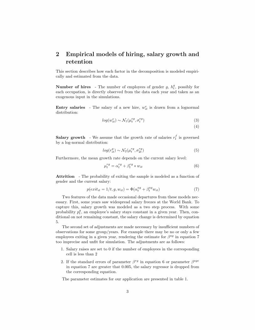
2 Empirical models of hiring, salary growth andretention

This section describes how each factor in the decomposition is modeled empiri-cally and estimated from the data.

Number of hires - The number of employees of gender g, hgt , possibly foreach occupation, is directly observed from the data each year and taken as anexogenous input in the simulations.

Entry salaries - The salary of a new hire, weit is drawn from a lognormal

distribution:

log(weit) ∼ N1(µeg

t , σegt ) (3)

(4)

Salary growth - We assume that the growth rate of salaries rft is governedby a log-normal distribution:

log(rgit) ∼ N2(µrgt , σ

rg2t ) (5)

Furthermore, the mean growth rate depends on the current salary level:

µrgt = αrg

t + βrgt ∗ wit (6)

Attrition - The probability of exiting the sample is modeled as a function ofgender and the current salary:

p(exitit = 1/t, g, wit) = Φ(αagt + βag

t wit) (7)

Two features of the data made occasional departures from these models nec-essary. First, some years saw widespread salary freezes at the World Bank. Tocapture this, salary growth was modeled as a two step process. With someprobability pgt , an employee’s salary stays constant in a given year. Then, con-ditional on not remaining constant, the salary change is determined by equation5.

The second set of adjustments are made necessary by insufficient numbers ofobservations for some group/years. For example there may be no or only a fewemployees exiting in a given year, rendering the estimate for βag in equation 7too imprecise and unfit for simulation. The adjustments are as follows:

1. Salary raises are set to 0 if the number of employees in the correspondingcell is less than 2

2. If the standard errors of parameter βrg in equation 6 or parameter βage

in equation 7 are greater that 0.005, the salary regressor is dropped fromthe corresponding equation.

The parameter estimates for our application are presented in table 1.

3

Table 1: Parameter estimates (averaged for cells containing at least 10observations)

pgt αrgt βrg

t βagt αag

t hgt µegt σeg

t

Male - I - GA-GE 0.0574 -2.8287 0.5967 0.0003 0.1449 325 30.4358 9.5392Male - II - GA-GE 0.0497 -2.7894 0.5336 0.0001 0.0964 282 27.0642 7.6398Female - I - GA-GE 0.0517 -2.8822 0.5455 -0.0017 0.1301 428 27.1002 6.1420Female - II - GA-GE 0.0592 -2.8829 0.5802 -0.0005 0.1074 335 25.1812 4.6313Male - I - GF+ 0.0326 -2.9093 0.4976 -0.0012 0.0845 203 67.0187 9.6568Male - II - GF+ 0.0389 -2.8850 0.5031 -0.0009 0.0673 129 53.0608 5.6551Female - I - GF+ 0.0374 -2.8844 0.4953 0.0001 0.0542 56 52.1491 6.2589Female - II - GF+ 0.0446 -2.8262 0.5221 -0.0007 0.0468 24 51.0044 4.6852Source:

3 Simulation algorithm

Given the estimated models above, the simulation algorithm updates salariesfrom year t− 1 to year t as follows:

1. Store the simulated annual salaries carried over from t− 1 as a histogramwith bin size of 1000 dollars.

2. For each bin in the histogram, and for each individual in the bin, draw asalary from a uniform distribution over the support of the bin, and a rateat which that salary increases during year t using the fitted value fromequation 6. Then determine the new bin in which that individual belongsafter the salary raise.

3. Determine for each employee whether they exit the sample at the end oft using the probability obtained from equation 7.

4. Build a histogram of entry salaries for each gender and each employeegroup using the number of hires for that group and the distribution of entrysalaries in equation 3. Add the histogram of entrants to the histogram ofemployees who didn’t exit.

5. Go to t+ 1.

4 Simulation fit

We apply this procedure taking 1987 as the initial year and simulating forwardto 2015. We then compare the simulated 2015 distribution of salaries with itsdata counterpart for each group of employee.

Figures 1 and 2 present the difference between the mean and the standarddeviations of the distribution of salaries of each group of employees in the dataand the simulations in 2015.

4

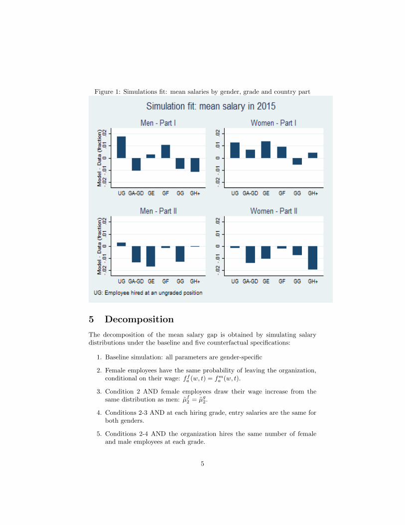
Figure 1: Simulations fit: mean salaries by gender, grade and country part

5 Decomposition

The decomposition of the mean salary gap is obtained by simulating salarydistributions under the baseline and five counterfactual specifications:

1. Baseline simulation: all parameters are gender-specific

2. Female employees have the same probability of leaving the organization,conditional on their wage: ffa (w, t) = fma (w, t).

3. Condition 2 AND female employees draw their wage increase from thesame distribution as men: µ̃f

2 = µ̃g2.

4. Conditions 2-3 AND at each hiring grade, entry salaries are the same forboth genders.

5. Conditions 2-4 AND the organization hires the same number of femaleand male employees at each grade.

5

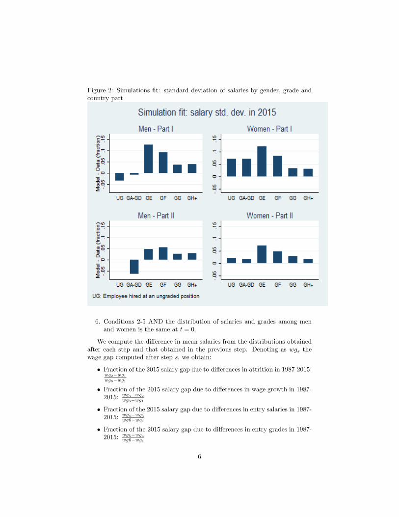
Figure 2: Simulations fit: standard deviation of salaries by gender, grade andcountry part

6. Conditions 2-5 AND the distribution of salaries and grades among menand women is the same at t = 0.

We compute the difference in mean salaries from the distributions obtainedafter each step and that obtained in the previous step. Denoting as wgs thewage gap computed after step s, we obtain:

• Fraction of the 2015 salary gap due to differences in attrition in 1987-2015:wg2−wg1wg6−wg1

• Fraction of the 2015 salary gap due to differences in wage growth in 1987-2015: wg3−wg2

wg6−wg1

• Fraction of the 2015 salary gap due to differences in entry salaries in 1987-2015: wg4−wg3

wg6−wg1

• Fraction of the 2015 salary gap due to differences in entry grades in 1987-2015: wg5−wg4

wg6−wg1

6

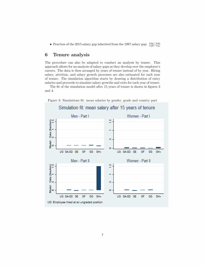
• Fraction of the 2015 salary gap inherited from the 1987 salary gap: wg6−wg5wg6−wg1

6 Tenure analysis

The procedure can also be adapted to conduct an analysis by tenure. Thisapproach allows for an analysis of salary gaps as they develop over the employee’scareers. The data is then arranged by years of tenure instead of by year. Hiringsalary, attrition, and salary growth processes are also estimated for each yearof tenure. The simulation algorithm starts by drawing a distribution of entrysalaries and proceeds to simulate salary growths and exits for each year of tenure.

The fit of the simulation model after 15 years of tenure is shown in figures 3and 4.

Figure 3: Simulations fit: mean salaries by gender, grade and country part

7

Figure 4: Simulations fit: standard deviation of salaries by gender, grade andcountry part

8