Workspace Analysis of a Linear Delta Robot: Calculating ...
79
Rose-Hulman Institute of Technology Rose-Hulman Scholar Graduate eses - Mechanical Engineering Mechanical Engineering Fall 11-2014 Workspace Analysis of a Linear Delta Robot: Calculating the Inscribed Radius Michael Louis Pauly Follow this and additional works at: hp://scholar.rose-hulman.edu/ mechanical_engineering_grad_theses Part of the Other Mechanical Engineering Commons is esis is brought to you for free and open access by the Mechanical Engineering at Rose-Hulman Scholar. It has been accepted for inclusion in Graduate eses - Mechanical Engineering by an authorized administrator of Rose-Hulman Scholar. For more information, please contact [email protected]. Recommended Citation Pauly, Michael Louis, "Workspace Analysis of a Linear Delta Robot: Calculating the Inscribed Radius" (2014). Graduate eses - Mechanical Engineering. Paper 1.
Transcript of Workspace Analysis of a Linear Delta Robot: Calculating ...

Rose-Hulman Institute of TechnologyRose-Hulman Scholar
Graduate Theses - Mechanical Engineering Mechanical Engineering
Fall 11-2014
Workspace Analysis of a Linear Delta Robot:Calculating the Inscribed RadiusMichael Louis Pauly
Follow this and additional works at: http://scholar.rose-hulman.edu/mechanical_engineering_grad_theses
Part of the Other Mechanical Engineering Commons
This Thesis is brought to you for free and open access by the Mechanical Engineering at Rose-Hulman Scholar. It has been accepted for inclusion inGraduate Theses - Mechanical Engineering by an authorized administrator of Rose-Hulman Scholar. For more information, please [email protected].
Recommended CitationPauly, Michael Louis, "Workspace Analysis of a Linear Delta Robot: Calculating the Inscribed Radius" (2014). Graduate Theses -Mechanical Engineering. Paper 1.

Workspace Analysis of a Linear Delta Robot:
Calculating the Inscribed Radius
A Thesis
Submitted to the Faculty
of
Rose-Hulman Institute of Technology
by
Michael Louis Pauly
In Partial Fulfillment of the Requirements for the Degree
of
Master of Science in Mechanical Engineering
November 2014
© 2014 Michael Louis Pauly

ii

ABSTRACT
Pauly, Michael Louis
M.S.M.E.
Rose-Hulman Institute of Technology
November 2014
Workspace Analysis of a Linear Delta Robot: Calculating the Inscribed Radius
Thesis Advisor: Dr. Dave Fisher
One of the most important traits of a robotic manipulator is its work envelope, the space
in which the robot can position its end effector. Parallel manipulators, while generally faster, are
restricted by smaller work envelopes [1]. As such, understanding the parameters defining a
physical robot’s work envelope is essential to the optimal design, selection, and use of robotic
parallel manipulators.
A Linear Delta Robot (LDR) is a type of parallel manipulator in which three prismatic
joints move separate arms which connect to a single triangular end plate [2]. In this study,
general inverse kinematics were derived for a linear delta robot. These kinematics were then
used to determine the reachable points within a plane in the robot’s work envelope, incorporating
the physical constraints imposed by a real robot. After simulating several robots of varying
parameters, a linear regression was performed in order to relate the robot’s physical parameters
to the inscribed radius of the area reachable in a plane of the LDR’s work envelope. Finally, a

iv
physical robot was constructed and used as a reality check to confirm the kinematics and
inscribed radius.
This study demonstrates the relationship between the LDR’s physical dimensions and the
inscribed radius of its work envelope. Building a physical robot allowed confirmation of the
resulting equation, validating an accurate representation of the LDR’s physical constraints. By
doing so, the resulting equation provides a powerful tool for correctly sizing a LDR based on a
desired work envelope.

ACKNOWLEDGEMENTS
I would like to thank the following persons for sharing their expertise, kind words, and
motivation, without whom it is unlikely that this thesis would ever have been written.
In no particular order:
Dr. Dave Fisher
Dr. Carlotta Berry
Dr. Jerry Fine
Jerry Leturgez
Ron Hofmann
Tom Rogge
The Rose-Hulman Robotics Team


1
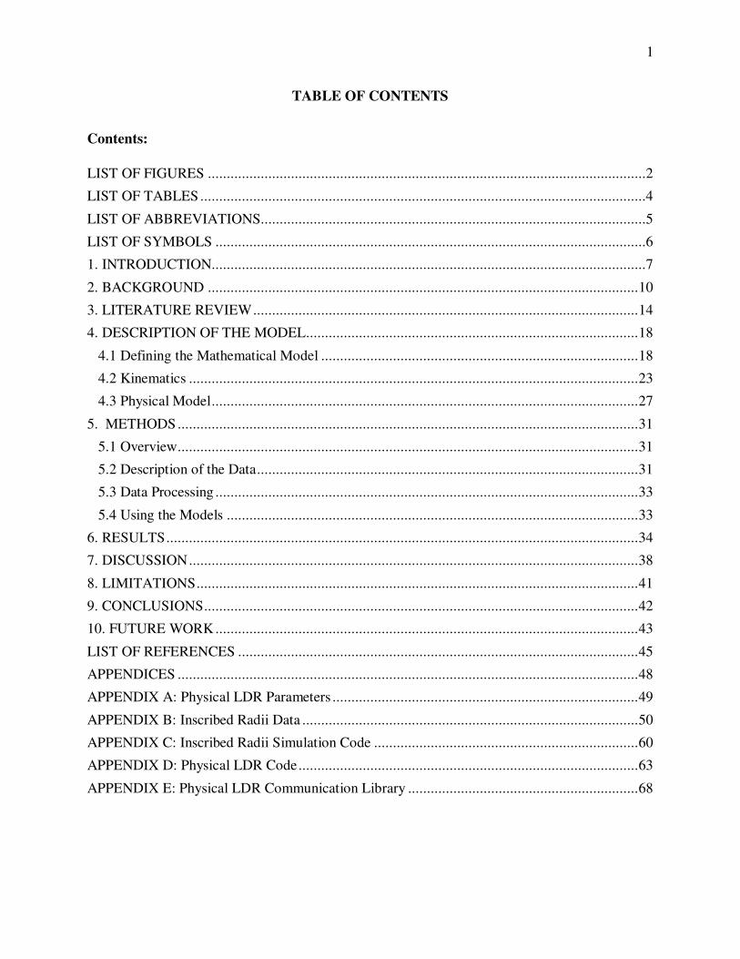
TABLE OF CONTENTS
Contents:
LIST OF FIGURES ....................................................................................................................2
LIST OF TABLES ......................................................................................................................4
LIST OF ABBREVIATIONS......................................................................................................5
LIST OF SYMBOLS ..................................................................................................................6
1. INTRODUCTION...................................................................................................................7
2. BACKGROUND .................................................................................................................. 10
3. LITERATURE REVIEW ...................................................................................................... 14
4. DESCRIPTION OF THE MODEL ........................................................................................ 18
4.1 Defining the Mathematical Model .................................................................................... 18
4.2 Kinematics ....................................................................................................................... 23
4.3 Physical Model ................................................................................................................. 27
5. METHODS .......................................................................................................................... 31
5.1 Overview .......................................................................................................................... 31
5.2 Description of the Data ..................................................................................................... 31
5.3 Data Processing ................................................................................................................ 33
5.4 Using the Models ............................................................................................................. 33
6. RESULTS ............................................................................................................................. 34
7. DISCUSSION ....................................................................................................................... 38
8. LIMITATIONS ..................................................................................................................... 41
9. CONCLUSIONS ................................................................................................................... 42
10. FUTURE WORK ................................................................................................................ 43
LIST OF REFERENCES .......................................................................................................... 45
APPENDICES .......................................................................................................................... 48
APPENDIX A: Physical LDR Parameters ................................................................................. 49
APPENDIX B: Inscribed Radii Data ......................................................................................... 50
APPENDIX C: Inscribed Radii Simulation Code ...................................................................... 60
APPENDIX D: Physical LDR Code .......................................................................................... 63
APPENDIX E: Physical LDR Communication Library ............................................................. 68

2
LIST OF FIGURES
Figure 1: A Linear Delta Robot ...................................................................................................7
Figure 2: Inscribed Radius of a LDR Work Envelope ..................................................................8
Figure 3: Example Work Envelope of a Serial Manipulator [9] ................................................. 11
Figure 4: The Stewart Platform [13] .......................................................................................... 12
Figure 5: A Diagram of the Delta Robot from the Original 1990 Patent [3] ............................... 14
Figure 6: Clavel's Linear Delta Design [3] ................................................................................. 15
Figure 7: Linear Delta Robot 3-D Printer [15] ........................................................................... 16
Figure 8: The LDR Model Used by Miller and Stock [4] ........................................................... 17
Figure 9: Modeling LDRs with 3 Spheres [4] ............................................................................ 17
Figure 10: Location and Orientation of the Coordinate System Origin ....................................... 18
Figure 11: Defining Joint Axis Offsets ...................................................................................... 19
Figure 12: Top View of the LDR’s Default Position .................................................................. 20
Figure 13: �� Measured with regard to �� ................................................................................. 21
Figure 14: Side View of the LDR with Parameters .................................................................... 22
Figure 15: All Possible LDR Poses for a Reachable Position [4] ............................................... 26
Figure 16: The Constructed LDR .............................................................................................. 27
Figure 17: Rotation Limits on the Spherical Joints .................................................................... 28
Figure 18: Spherical Joints on the Delta Plate ............................................................................ 29
Figure 19: Pointer used as an End Effector ................................................................................ 29
Figure 20: Limit Switches for the Prismatic Joints ..................................................................... 30
Figure 21: MATLAB Plot of Unreachable Points and the Inscribed Radius ............................... 32
Figure 22: Expected Workspace of the Physical LDR ................................................................ 36

3
Figure 23: Positional Results on the Physical LDR .................................................................... 39
Figure 24: Positional Results within the Work Envelope ........................................................... 40

4
LIST OF TABLES
Table 1: t Scores for Angular Terms ...................................................................................... 34
Table 2: Linear Regression Results ........................................................................................ 35
Table 3: Linear LDR Position Testing ................................................................................... 37
Table 4: ψ Values .................................................................................................................... 43

5
LIST OF ABBREVIATIONS
EE: End Effector
EoAT: End of Arm Tooling
LDR: Linear Delta Robot
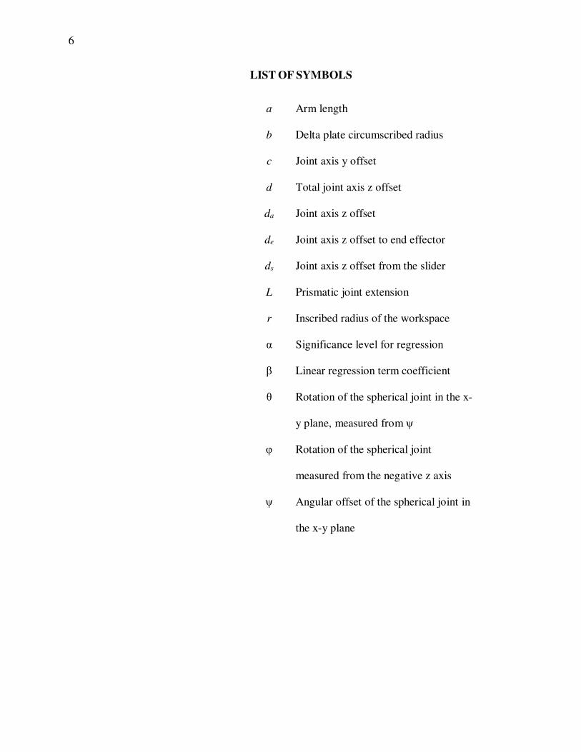
6
LIST OF SYMBOLS
a Arm length
b Delta plate circumscribed radius
c Joint axis y offset
d Total joint axis z offset
da Joint axis z offset
de Joint axis z offset to end effector
ds Joint axis z offset from the slider
L Prismatic joint extension
r Inscribed radius of the workspace
α Significance level for regression
β Linear regression term coefficient
θ Rotation of the spherical joint in the x-
y plane, measured from ψ
φ Rotation of the spherical joint
measured from the negative z axis
ψ Angular offset of the spherical joint in
the x-y plane
7
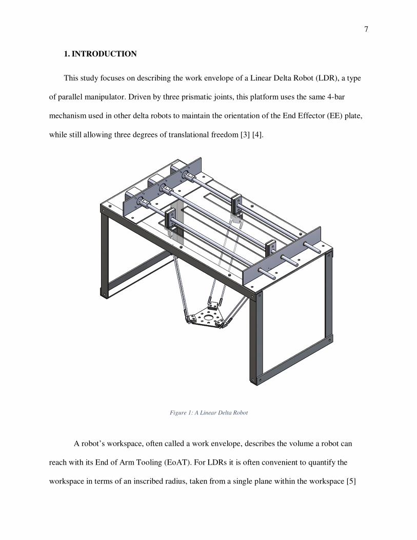
1. INTRODUCTION
This study focuses on describing the work envelope of a Linear Delta Robot (LDR), a type
of parallel manipulator. Driven by three prismatic joints, this platform uses the same 4-bar
mechanism used in other delta robots to maintain the orientation of the End Effector (EE) plate,
while still allowing three degrees of translational freedom [3] [4].
Figure 1: A Linear Delta Robot
A robot’s workspace, often called a work envelope, describes the volume a robot can
reach with its End of Arm Tooling (EoAT). For LDRs it is often convenient to quantify the
workspace in terms of an inscribed radius, taken from a single plane within the workspace [5]

8
[6]. Measuring this radius is a simple task on a physical LDR but difficult to calculate for a
theoretical robot [7]. The objective of this study is to determine the relationship between the
inscribed radius of a LDR’s workspace and the robot’s physical parameters. Figure 2 shows the
LDR from Figure 1 when viewed from the right. The LDR’s work envelope is shown in blue,
with the inscribed radius shown as the red arrow.
Figure 2: Inscribed Radius of a LDR Work Envelope
One objective of this study is to place an emphasis on studying the physical workspace of
a LDR, rather than the theoretical workspace, so additional factors such as joint angle limits and
9
end effector mounting are considered. Using the calculated inverse kinematics, a simulation
program was written to measure the inscribed radius empirically using several different sets of
physical parameters. A linear regression was performed comparing the arm length, delta plate
radius, joint axis offsets, and spherical joint limits to the inscribed radius, resulting in an equation
defining the inscribed radius in terms of the physical parameters of a LDR. Finally, a physical
LDR was built to test the inverse kinematics and measure the inscribed radius. This platform was
essential to confirm the kinematics and ensure that the assumptions about physical constraints
made in the mathematical model were valid, acting as a reality check for the simulation.
The single resulting equation can be used to evaluate a Linear Delta Robot’s work
envelope inscribed radius based only on easily measurable physical characteristics of the robot.
No kinematic equations are required, meaning that this equation can be used quickly without
requiring iterations to evaluate several possible robots quickly. Thus, the found equation is a
powerful tool for easily approximating the inscribed radius of a Linear Delta Robot.

10
2. BACKGROUND
In recent years, robotic manipulators have gained popularity in many industries. Providing
high strength, speed, repeatability, and robustness, robots have gained widespread acceptance for
jobs deemed too labor-intensive, dangerous, monotonous, or difficult for humans. The growing
number of robot models and manufacturers means that users have a plethora of potential robotic
candidates for any task, making the selection of an ideal robot a difficult task.
A defining characteristic of any robotic manipulator is its work envelope. This term refers
to any point that the robot can reach with its EoAT. Because the work envelope represents the
space in which the robot can effectively interact with the environment, it is an essential aspect to
consider when selecting or placing a robot. Designing a robot for a prescribed workspace can be
an especially difficult problem, depending on the manipulator in question [8]. It is important to
note that generally the work envelope only considers the EoAT position, but not orientation.
Many times a robot will be able to reach a location, but cannot interact with a part or fixture
because it has the wrong orientation. While work envelopes are a three dimensional space, they
are often described with a radius (or radii) within a cross-sectional plane, as seen in Figure 3.

11
Figure 3: Example Work Envelope of a Serial Manipulator [9]
An essential tool for describing a robot’s position are forward and inverse kinematics [10].
Forward kinematics are used to determine a robot’s end effector position based on the state of the
robots actuators. Inverse kinematics are used to calculate the required actuator states to achieve a
desired end position. Depending on the manipulator in question, both the forward and inverse
kinematics may provide multiple solutions. All valid actuator configurations which reach a
single end point are the set of viable poses. Serial manipulators generally have a unique solution
to the forward kinematics problem, while having multiple poses which satisfy the inverse
kinematics. Parallel manipulators, depending on the type, can have numerous solutions to both
forward and inverse kinematics [11]. The Stewart Platform, shown in Figure 4 below, has 40
direct forward kinematic solutions [12].

12
Figure 4: The Stewart Platform [13]
Robotic manipulators are generally categorized into one of two groups: serial and parallel
[12]. Serial robots have one path of joints and links from the base to the end effector, whereas
parallel robots have multiple paths from the base to the end effector. In general, serial
manipulators are heavier and slower because each joints’ motor must be mounted on the arm (or
have motion transmitted via some physical linkage), but have larger work envelopes. Parallel
manipulators are usually faster, as their motors are housed in the stationary base, but have
smaller work envelopes [14]. As such, when using parallel manipulators it is essential to select
the correct robot in order to make full use of the work envelope.
Another significant difference between serial and parallel manipulators is the way in which
their kinematics are derived. Serial manipulators often use coordinate transformations, in the
form of matrices, to relate the position of each link to the previous one [10]. Thus, the end
position, expressed as a vector, is found by multiplying the initial position by the transformation
matrices for each link. Many transformations are used, one of the most popular being the

13
Denavit-Hartenberg method. If the full transformation matrix is invertible, then the inverse
kinematics is performed by multiplying the desired position by the inverted transformation
matrix. This method is limited to a single solution and does not provide multiple poses.
Oh the other hand, parallel manipulators are modeled by systems of equations. Starting at
the base, the end position is expressed with regards to the position of each kinematic chain in the
robot. For inverse kinematics, the system of equations is solved to determine the required
actuator inputs. This proves to be a difficult task, with each manipulator often requiring its own
method [5] [11] [12].

14
3. LITERATURE REVIEW
One of the most popular parallel manipulator designs is the DELTA platform, originally
developed by Swiss team lead by Reymond Clavel [3]. Driven by three revolute joints located on
the base, motion is transmitted through three parallelogram arms to a semi-triangular end piece,
called the delta plate. One of Clavel’s models, shown in Figure 5 below, has a fourth revolute
joint that allows for rotation of the End Effector about the Z axis.
Figure 5: A Diagram of the Delta Robot from the Original 1990 Patent [3]

15
The defining aspect of Delta manipulators are their parallelogram arms. Two long links are
connected to the adjoining links by spherical joints at each end, forming a 4-bar mechanism. This
setup ensures that the two connected links remain parallel, effectively removing one degree of
freedom from the system. By using three 4-bar mechanisms, Delta platforms lock the pitch, roll,
and yaw of the Delta plate, such that the end effector has a constant orientation regardless of
position.
There are various Delta platform configurations, including linear Delta robots, which swap
the revolute joints of the original Delta platform for prismatic joints. In most cases, motion is
achieved through the use of lead screws and rotational motors, though other linear actuation
methods are also used. Figure 6 shows a linear delta platform designed by Clavel. Because of
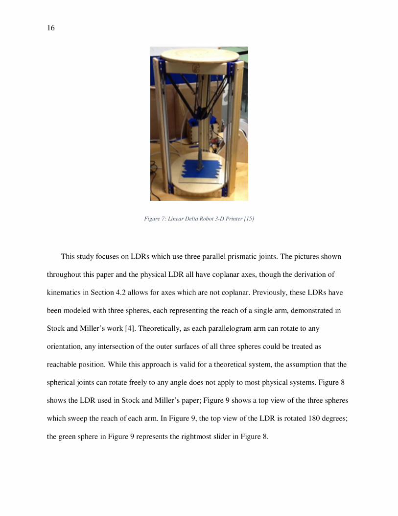
their high accuracy and rigidity, LDRs are sometimes used for 3-D printing, as seen in Figure 7.
Figure 6: Clavel's Linear Delta Design [3]
16
Figure 7: Linear Delta Robot 3-D Printer [15]
This study focuses on LDRs which use three parallel prismatic joints. The pictures shown
throughout this paper and the physical LDR all have coplanar axes, though the derivation of
kinematics in Section 4.2 allows for axes which are not coplanar. Previously, these LDRs have
been modeled with three spheres, each representing the reach of a single arm, demonstrated in
Stock and Miller’s work [4]. Theoretically, as each parallelogram arm can rotate to any
orientation, any intersection of the outer surfaces of all three spheres could be treated as
reachable position. While this approach is valid for a theoretical system, the assumption that the
spherical joints can rotate freely to any angle does not apply to most physical systems. Figure 8
shows the LDR used in Stock and Miller’s paper; Figure 9 shows a top view of the three spheres
which sweep the reach of each arm. In Figure 9, the top view of the LDR is rotated 180 degrees;
the green sphere in Figure 9 represents the rightmost slider in Figure 8.

17
Figure 8: The LDR Model Used by Miller and Stock [4]
Figure 9: Modeling LDRs with 3 Spheres [4]
This method does illustrate the possibility for multiple poses, as any intersection between
three spheres will be a valid solution. In rare cases, one sphere will lie tangent to the intersection
of the two other spheres, resulting in a single unique solution. If two spheres do not intersect,
then no solution exists.

18
4. DESCRIPTION OF THE MODEL
4.1 Defining the Mathematical Model
In order to accurately predict the work envelope of a real LDR, a new model which includes
physical constraints is required. The model used in this study will focus primarily on the
restriction of the position of the spherical joints, while also accounting for the end effector
mounting and the coupling of the prismatic and spherical joints.
To begin, a Cartesian coordinate system is created, and attached to the base of the LDR as
shown below in Figure 10.
Figure 10: Location and Orientation of the Coordinate System Origin
Next, the physical parameters of the LDR are mapped to variables. This study uses the
following convention: constant lengths are assigned lowercase letters, actuator variables are
x
y
z

19
assigned uppercase letters, and angular measurements are assigned Greek letters. Subscripts
indicate the kinematic path (joint axis) associated with the variable. Joint axis 1 is the lower left
prismatic joint, joint axis 2 is the center joint, and joint axis 3 is the far joint. The y and z
direction offsets, �� and ���, respectively, for each axis are shown in Figure 11. For the LDR
constructed in this study, ��� is zero for all axes.
Figure 11: Defining Joint Axis Offsets
Each prismatic joint is a slider which connects to the 4-bar mechanism via spherical
joints. The slider’s x displacement is ��, measured from the y-z plane, shown above. Because the
two arms in each 4-bar mechanism have a constant length and are always parallel, they are
modelled as a single link of length a. This study uses three angles to describe the rotation of the
��� 0
�� �� ��

20
spherical joint. In order to measure the same angular displacement for each of the links, an
angular offset, ��, is used. �� is the rotation from a hypothetical spherical joint facing along the
positive x axis. This constant is used to define the base or zero position of each upstream
spherical joint. ��, the lateral rotation of each spherical joint, is then measured from �� in the x-y
plane. By using ��, it is possible to directly compare the �� values of each joint and determine if
they exceed the possible rotation of the physical joints. Figure 12 shows the angular offsets, and
Figure 13 shows an example �� value measured from one of these offsets.
Figure 12: Top View of the LDR’s Default Position
��
��
� �

21
Figure 13: �� Measured with regard to ��
The third angle measured, ��, measures the 4-bar mechanisms’ rotation from the negative
z axis. Length b is the horizontal distance from the center of the delta plate to the center of the
downstream spherical joint. Two additional z offsets are also needed. The distance from the
prismatic joint’s axis to the spherical joint is designated ���; the distance from the downstream
spherical joint to the end effector is labelled ��� . Figure 14 shows the z distance offsets, using the
bottom of the delta plate as the end effector in the simulations. For the constructed LDR, a
pointer was made to extend below the bottom of the delta plate to allow easy measurement to the
center.
��

22
Figure 14: Side View of the LDR with Parameters
To simplify future equations, a single parameter, ��, will be used as the z offset, as
defined in Equation 1 below.
�� ��� � ��� � ��� (1)
Of particular concern to this study are b, effective radius of the delta plate, c, the y offset
of the joint axes, and θ and φ, angles which describe the spherical joints. These parameters are
often ignored in other analyses but are important when considering an actual robot. Depending
on the desired size of the end effector its required mounting footprint, the radius of the delta plate
might be substantial or at least nontrivial. Additionally, few spherical joints exist that provide
unlimited rotation in all three directions, so limiting the allowable ranges of θ and φ will more
closely model physical systems.
��
�
���
���
�

23
4.2 Kinematics
Finding the forward kinematic equations is straightforward. Following the kinematic
chain from the origin to the end position for each axis gives the following result:
� �� � � cos���� � � cos��� � ��� sin���� (2)
� �� � � sin���� � � sin��� � ��� sin���� (3)
� �� − �cos���� (4)
Because the three equations above apply to each axis, there are nine equations to solve
for the nine unknown parameters (L, φ, and θ for each axis). However, as each joint axis is
independent and can be solved individually, we can consider each axis as its own three degree of
freedom system.
Solving for inverse kinematic equations is accomplished by rearranging the forward
kinematic equations. Beginning with Equation 4, it is a simple matter to solve for ��.
�� cos!� "�� − �� # (5)
With �� known, Equation 3 could be rearranged to isolate ��, then solved by substituting
Equation 5 for ��. However, that would result in the use of an inverse sine function. Previous
experience has shown that MATLAB’s inverse sine function is unreliable for four-quadrant
solving. Thus, another method is used, utilizing MATLAB’s more robust, four-quadrant inverse
tangent function. This requires defining a quantity in terms of its sine and cosine. In order to
accomplish this, Equations 2 and 3 are rearranged as shown.

24
�−�� − � cos���� � cos��� � ��� sin���� (6)
�−�� − � sin���� � sin��� � ��� sin���� (7)
Equations 6 and 7 can be solved for cos��� � ��� and sin��� � ���, but Li is still
unknown and must be solved for first. This is done by squaring Equations 6 and 7, then adding
them together, resulting in Equation 8.
��−�� − � cos����� � ��−�� − � sin����� � cos��� � ��� sin���� +� sin��� � ��� sin����
(8)
Applying the trigonometric identity in Equation 9 to Equation 8 provides a quadratic
equation with Li as the only unknown.
cos��� � ��� � sin��� � ��� 1 (9)
��−�� − � cos����� � ��−�� − � sin�����
� sin���� (10)
Solving Equation 10 yields the final equation for Li.
�� � − � cos����
± &� sin���� − ��−�� − � sin�����
(11)
With Li solved for, Equations 6 and 7 can be rearranged as shown below, then used to
solve for �� with MATLAB’s atan2 function.

25
cos��� � ��� ��−�� − � cos�����
�sin���� (12)
sin��� � ��� ��−�� − � sin�����
�sin���� (13)
�� �'�(2�sin��� � ��� , cos��� � ���� − �� (14)
Thus, Equations 5, 11, and 14 model the inverse kinematics for a LDR. Three
characteristics of these equations are worth noting. First, the angle �� only varies with z position.
Because of this, if �� is the same for all three joint axes, then the magnitude of �� will be the
same (this study assumes that a is constant for all joint axes). Next, each of the equations can
provide complex solutions, either from a trigonometric inverse or the square root of a negative
number. In either case, a complex solutions signifies that the position in question would be
unreachable for a physical robot. Finally, each equation can be solved to provide two solutions.
For Equations 5 and 14, the two solutions arise from the inverse trigonometric functions when
their ranges are extended to –π to π. In Equation 11, the two solutions come from the positive
and negative values that can be the result of the square root terms. The two possible states for
each axis allow for a total of eight (2�) possible robot poses for a single desired position. Stock
and Miller provide an excellent illustration of the eight possible poses:

26
Figure 15: All Possible LDR Poses for a Reachable Position [4]
For this study, the pose in the upper left is chosen, so that � is always greater than �� and ��. This choice was made primarily to accommodate the physical robot, which has ψ angles
most similar to those shown. Thus, the inverse kinematic equations for ��,� , and �� become:
�� � − � cos���� − &� sin���� − ��−�� − � sin����� (15)
� � − � cos�� � � &� sin�� � − ��−� − � sin�� �� (16)
�� � − � cos���� − &� sin���� − ��−�� − � sin����� (17)
27
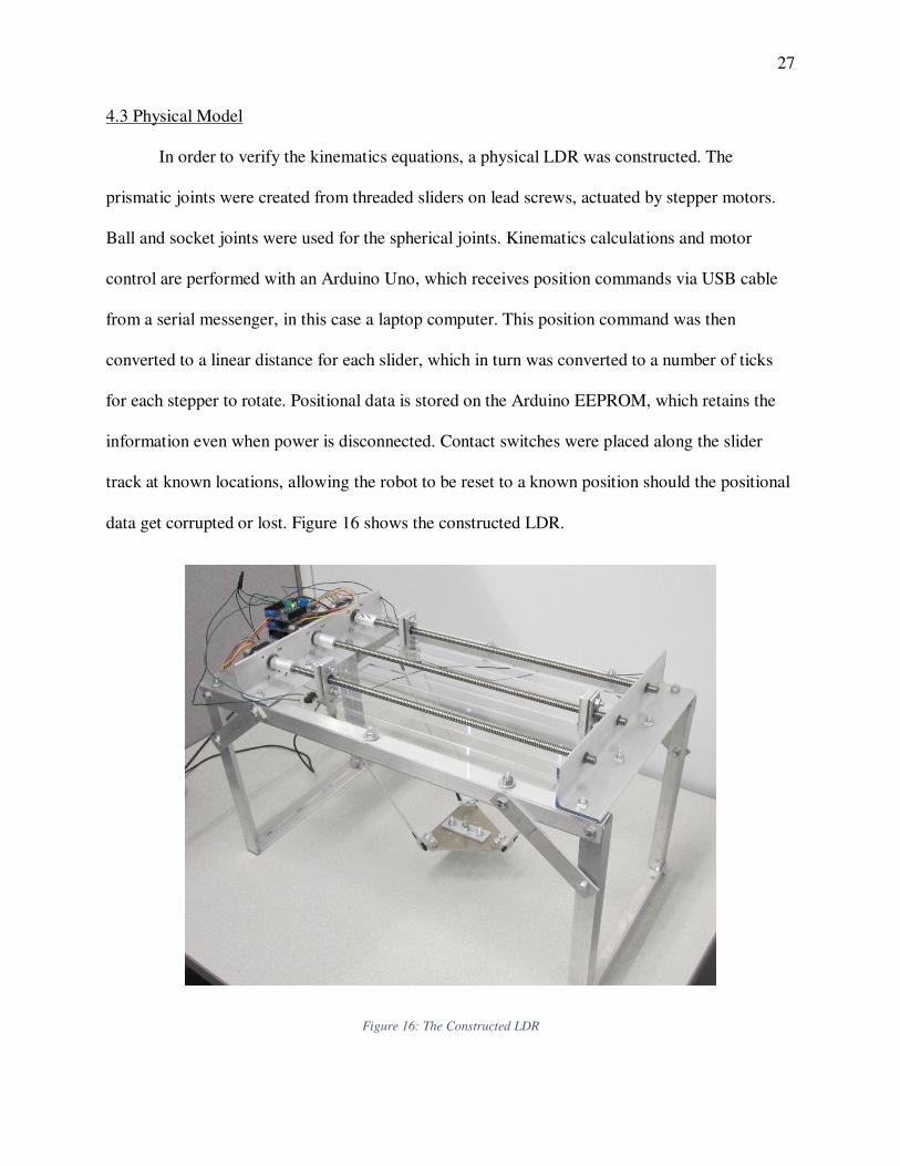
4.3 Physical Model
In order to verify the kinematics equations, a physical LDR was constructed. The
prismatic joints were created from threaded sliders on lead screws, actuated by stepper motors.
Ball and socket joints were used for the spherical joints. Kinematics calculations and motor
control are performed with an Arduino Uno, which receives position commands via USB cable
from a serial messenger, in this case a laptop computer. This position command was then
converted to a linear distance for each slider, which in turn was converted to a number of ticks
for each stepper to rotate. Positional data is stored on the Arduino EEPROM, which retains the
information even when power is disconnected. Contact switches were placed along the slider
track at known locations, allowing the robot to be reset to a known position should the positional
data get corrupted or lost. Figure 16 shows the constructed LDR.
Figure 16: The Constructed LDR

28
As stated previously, a goal of this study is to determine an equation for inscribed radius
which accounts for physical limitations of a system. As such, certain attributes of the LDR were
chosen to be less than ideal. The delta plate is larger than necessary to hold the EoAT used, to
allow for potentially larger tooling. The ball and socket joints that were chosen had a notable
restriction on φ rotation, as shown in Figures 17 and 18 below. A complete table of the
constructed LDR properties can be found in Appendix A.
Figure 17: Rotation Limits on the Spherical Joints
29
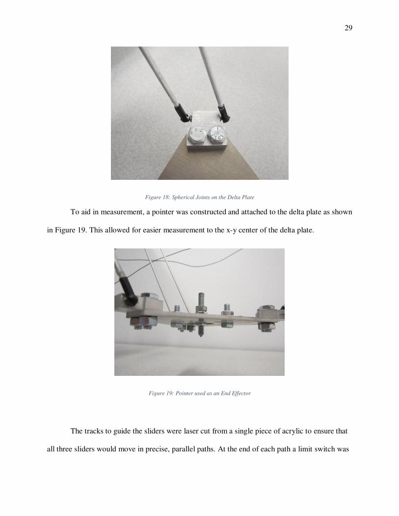
Figure 18: Spherical Joints on the Delta Plate
To aid in measurement, a pointer was constructed and attached to the delta plate as shown
in Figure 19. This allowed for easier measurement to the x-y center of the delta plate.
Figure 19: Pointer used as an End Effector
The tracks to guide the sliders were laser cut from a single piece of acrylic to ensure that
all three sliders would move in precise, parallel paths. At the end of each path a limit switch was

30
installed. The purpose of these switches, seen in Figure 20, was twofold. First, they allow for
recalibrating of each prismatic joint’s length. Second, they keep each slider out of the danger
zone at the end of the track, in which the sliders could hit the end of the track cause the couplers
to slip, and thus cause the lead screws to slip and lose position.
Figure 20: Limit Switches for the Prismatic Joints

31
5. METHODS
5.1 Overview
One can see from Equation 2 that the LDR’s reach in the x direction is primarily driven by
the positions of the three prismatic joints. To increase the LDR’s reach in the x direction, one can
simply increase the travel of the prismatic joints. However, the LDR’s reach in the y and z
directions is based on the arm length, delta plate size, joint axis offsets, and angles of the
spherical joints, whose interactions are not nearly as intuitive. This study therefore focuses on the
points reachable in a y-z plane at a fixed x value. Due to the nature of the LDR, the reachable
points in the plane will form a rough semicircle, the minimum radius of which will be the
inscribed radius for that set of physical parameters.
The radii found, in conjunction with their corresponding physical parameters, were then
used in a linear regression model to determine the equation predicting the inscribed radius. The
resulting coefficients then yielded an equation relating inscribed radius to the physical
parameters in the form shown below in Equation 18.
+ ,- � ,�� � , b � ,�c � ,/�0�1 � ,2�0�1 (18)
5.2 Description of the Data
Several values of a, b, and c, were chosen for testing, along with different allowable ranges
for � and θ, called �0�1 and �0�1, respectively. For each combination of these five physical
parameters, a MATLAB program was written to test a grid of points with the inverse kinematics
equations. Points within a y-z plane at a constant x value were tested. If the returned values for
��, ��, and �� were complex, or if �� or �� was outside range of �0�1 or �0�1 , then the point was

32
determined to be unreachable and stored. An origin point (not the robot system origin) was
selected to be the highest (greatest z value) point that lay along the centerline (the work envelope
was observed to be symmetric about the z axis). The inscribed radius was calculated as the
minimum distance from any unreachable to the origin, considering only points below the origin.
Figure 21, below, shows an example of the unreachable points (blue) and the inscribed radius
(red). This trial used di=-1, so points with a z value of -1 or higher were not calculated, as it was
already known that they would be unreachable.
Figure 21: MATLAB Plot of Unreachable Points and the Inscribed Radius
The inscribed radius r and the values of �, �, �, �0�1 , and �0�1 were stored for processing.
A complete table of the values for +, �, �, �, �0�1 , and �0�1 can be found in Appendix 2.
�
�

33
5.3 Data Processing
Linear regression was used to relate the inscribed radius r with �, �, �, �0�1 , and �0�1 .
Because �0�1 and �0�1 are angles, the values of sin��0�1�, cos��0�1�, sin��0�1�, and cos��0�1� were also considered. To determine which of the �0�1 and �0�1 terms to use, all possible
combinations of one �0�1 term and �0�1 term were tested. Any combination which had a
statistically insignificant term was eliminated. Of those combinations which remained, the
combination which had the largest absolute sum of t values was chosen. A significance level of
α=0.05 was chosen and a two-sided confidence interval was used.
With the proper angular terms selected, a final linear regression was performed to solve for
the coefficients in Equation 18. The same significance level of α=0.05 was used to determine
which terms, if any, were not statistically significant.
5.4 Using the Models
The models were used to predict the performance of the constructed LDR. Based on the
values shown in Appendix A the constructed LDR’s inscribed radius was calculated. Testing was
performed by selecting several points near the edge of the work envelope. The L1, L2, and L3
needed to reach these positions were calculated by the LDR’s Arduino controller and the LDR
was then moved to each position. The actual position of the EE was recorded and compared to
the expected values calculated by the MATLAB kinematics program.

34
6. RESULTS
Once the data was collected, nine linear regressions were performed to select the best
possible combination of �0�1 , cos��0�1�, or sin��0�1� and �0�1 , cos��0�1�, or sin��0�1�. For
each regression, the absolute sum of the t scores for the angular terms was computed. As seen
below in Table 1, the combination which most accurately represents the data is �0�1 and
cos��0�1�.
Table 1: t Scores for Angular Terms
�0�1 cos��0�1� sin��0�1�
�0�1 45.06 45.47 31.06
cos��0�1� 45.04 45.45 31.05
sin��0�1� 44.03 44.42 30.48
Thus, the terms �0�1 and cos��0�1� were selected and a final linear regression was
performed. The physical parameters, along with their β coefficients, significance levels, and t
values are shown below in Table 2.

35
Table 2: Linear Regression Results
Parameter β p t
Constant -1.3789 0.085 -1.72
a 0.3789 0.000 7.17
b 0.4742 0.000 5.18
c -0.5537 0.000 -6.05
�0�1 3.677 0.000 12.62
cos��0�1) -20.809 0.000 -32.85
Based on the p values for each term, all terms except the constant are statistically
significant. The linear regression resulted in an R-squared value of 77.23, meaning that over
three-quarters of the inscribed radius’s value is modelled by the given equation. Therefore, a best
estimate for the inscribed radius of a LDR’s workspace is
+ 0.3789� � 0.4742b − 0.5537c � 3.677�0�1 − 19.462cos��0�1) (19)
Based on this result, the inscribed radius for the constructed LDR was calculated to be
8.74 inches, compared to the 5.59 inches found by the MATLAB simulation, shown below in
Figure 22.
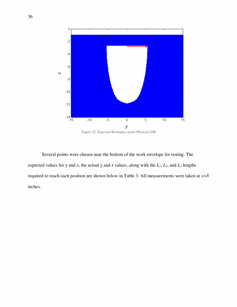
36
Figure 22: Expected Workspace of the Physical LDR
Several points were chosen near the bottom of the work envelope for testing. The
expected values for y and z, the actual y and z values, along with the L1, L2, and L3 lengths
required to reach each position are shown below in Table 3. All measurements were taken at x=8
inches.
�
�

37
Table 3: Linear LDR Position Testing
Expected y
(in)
Expected z
(in)
Measured y
(in)
Measured z
(in)
L1
(in)
L2
(in)
L3
(in)
-4 -10.5 -2.37 -10.94 2.7005 13.8345 6.4271
-3 -11 -1.88 -11.25 3.1032 13.6344 5.6543
-2 -11.4 -1.13 -11.5 3.6894 13.2594 5.6731
-1 -11.6 -0.75 -11.75 4.1425 13.1371 5.1036
0 -11.8 0 -11.81 5.434 12.3963 5.434
1 -11.6 0.69 -11.63 5.1036 13.1371 4.1425
2 -11.4 1.13 -11.5 5.6731 13.2594 3.6894
3 -11.0 1.75 -11.31 5.6543 13.6344 3.1032
4 -10.5 2.75 -10.94 6.4271 13.8345 2.7005

38
7. DISCUSSION
From Equation 19 it is immediately apparent that the cos��0�1) term immensely restricts the
inscribed radius. Especially for small manipulators, decreasing this term (by increasing �0�1)
should be the first step to increasing a LDR’s work envelope. As it exists in Equation 19, one
could theoretically increase the radius by causing �0�1 to cause cos��0�1) to become negative. In
practice, this would likely not add any benefit beyond being able to reach a point with a second
pose.
Interestingly, increasing the axis separation with c decreases the inscribed radius. Closer
axes allow for more movement, while spread axes restrict movement to points across the x-z
plane. However, close axes cause greater θ angles when moving at low φ angles near the x-z
plane, so care must be taken not to reduce c enough to lessen the inscribed radius.
As expected, increasing a increases the inscribed radius, as it directly contributes to a joint
axis’s reach in all directions. Surprisingly, b also has a positive impact on the inscribed radius,
and has close to the same impact as a. Initially, a large delta plate radius was thought to be a
detriment, causing more extreme φ and θ angles, but apparently the benefit of increased reach in
x and y had a greater impact on the radius. A large delta plate could still create issues in motor
positional or velocity control. Finally, because it directly affects the reach in z, increasing �0�1
also increases the radius.
The regression model is not accurate for all cases. The most obvious example that if
either of the joint limits were zero, a physical manipulator would have an inscribed radius of
zero, though the regression would predict a non-zero radius. This can also be seen with an arm
length of a = 0 or an axis separation of c = 0.

39
The positions of the physical LDR differed from the expected values largely due to
mechanical slop in the system, primarily due to the rotation of the sliders. While the tracks that
the sliders move along were intended to stop this, the semi-flexible acrylic did allow for some
rotation about the joint axis. Additionally, the acme nuts used on the lead screws were found to
have some wobble which allowed them to rotate along the axis. The ball and socket joints used
were composed of a metal ball within plastic socket. After some use, the plastic became mildly
worn down, which allowed a miniscule amount of linear movement as well as rotational
movement in the spherical joints. The combined effect of this variability lead to the delta plate
being pulled down (and thus inward) by gravity. Thus, all experimental results had y values
closer to zero and z values less than the predicted results, shown below in Figure 23.
Figure 23: Positional Results on the Physical LDR
�
�

40
Despite these issues, the physical LDR served as a successful sanity check to confirm that
the kinematics and work envelope calculations were roughly correct. The positional kinematics
were confirmed by moving the end effector to the expected position (by hand) without moving
the sliders, proving that the LDR could reach that position with the given L inputs. Figure 24
demonstrates this, showing that the experimental results still align with the predicted work
envelope.
Figure 24: Positional Results within the Work Envelope
�
�

41
8. LIMITATIONS
On the physical LDR, the largest limitation was the range of L. Because this range was
too small, points near the top of the work envelope could not be tested, meaning that the
inscribed radius could not be calculated as the origin could not be found. While unfortunate, this
oversight was not catastrophic as the LDR could still move around the bottom of the work
envelope, the most important and commonly used area. Additionally, the platform still acted as a
useful device to confirm the kinematics.

42
9. CONCLUSIONS
Despite some limitations, this study was largely successful in deriving the forward
kinematics, inverse kinematics, and an equation defining the inscribed radius for a LDR. While
the lower R-squared value indicates that the regression model does not capture all the variation
in the inscribed radius, Equation 19 still provides a powerful tool for estimating the inscribed
radius of a LDR. It affirms the importance of considering the impact of all the selected physical
parameters, and places heavy emphasis on the spherical joint angle restrictions. Using the
physical LDR as a reality check confirmed both the kinematics and the edge of the work
envelope, and was a valuable tool in understanding the capabilities and limitations of LDRs.
From the evidence shown, it should be clear that understanding and controlling the work
envelope is an essential step when designing or using a robotic manipulator. Hopefully, the
methods and equation presented in this thesis will provide insight to those attempting to
accurately define the workspace or kinematics of a linear delta robot.

43
10. FUTURE WORK
In order to improve the models, more physical LDRs should be constructed in order to
physically verify the equations. This study used a single LDR as a reality check, and while the
physical model roughly matched the equations, a single data point does not prove a trend. To
truly confirm the inscribed arc radius equation, an array of LDRs with varying parameters should
be built and tested, though this would obviously be a substantial investment of materials and
time.
Other future work could include LDRs with different ψ configurations. This study
exclusively used the ψ values shown in Table 4 below. These values were chosen to imitate
Clavel’s original delta manipulator by being even separated by ;� radians. However, due to the
nature of the 4-bar mechanisms on the arms, there is no reason that other ψ values could not
work.
Table 4: ψ Values
�� Value (rads)
1 �3
2 �
3 −�3
Additionally, while Clavel’s original design used constant values of a and b for all three
arms, Delta robots can be (and sometimes are) constructed with varying arm lengths and delta
plate sizes. As Equations 2, 3, and 4, show, each joint axis can be calculated independently, so

44
solving for LDRs that have differing a and b values for each joint would be a simple change that
could yield interesting results.
While this study focused on the inverse kinematics to find unreachable points, a robot’s
Jacobian matrix can also be used to find limits or singularities in a robot’s workspace. Some
attempts were made to derive a useful Jacobian from the inverse kinematics, but without success.
If a future study were to calculate the Jacobian, it might be more computationally efficient in
determining the unreachable points for the inscribed radius calculations. Additionally, the
Jacobian could provide information about areas within the workspace which would cause a LDR
to lose rigidity.
Finally, a more complex regression model could be attempted to find a more suitable
equation. This study did not include interaction terms or higher order terms in order to limit the
complexity, as the determination of the inscribed radius equation was done empirically.
However, looking at the inverse kinematics equations shows a number of interaction terms (some
with two-degree interactions), as well as higher order terms, so a more complex model could be
justified. Alternatively, an effort could be made to derive the inscribed radius equation entirely
from the kinematics.

45
LIST OF REFERENCES
[1] M. J. Uddin, S. Refaat, S. Nahavandi and H. Trinh, "Kinematic Modelling of a Robotic
Head with Linear Motors," Deakin University, School of Engineering and Technology,
Geelong.
[2] R. Clavel, "A Fast Robot with Parallel Geometry," in 18th International Symposium on
Industrial Robotics, Lausanne (Switzerland), 1998.
[3] R. Clavel, "Device for the positioning of an element in space". U.S. Patent 4,976,582, 11
Dec 1990.
[4] M. Stock and K. Miller, "Optimal Kinematic Design of Spatial Parallel Manipulators:
Application to the Linear Delta Robot," ASME Journal of Mechanical Design, vol. 125,
2003.
[5] Q. Yuan, S. Ji, Z. Wang, G. Wang, Y. Wan and L. Zhan, "Optimal Design of the Linear
Delta Robot for a Prescribed Cuboid Dexterous Workspace based on Performance Chart,"
in WSEAS Int. Conf. on Robotics, Control, and Manufacturing Technology, Hangzhou,
2008.
[6] X.-J. Liu, J. Wang, K.-K. Oh and J. Kim, "A New Approach to the Design of a DELTA
Robot with a Desired Workspace," Journal of Intelligent and Robotic Systems, vol. 39, pp.
209-225, 2004.

46
[7] Y. Zhao, "Dynamic optimum design of a three translational degrees of freedom parallel
robot while considering anisotrophic property," Robotics and Computer-Integrated
Manufacturing., vol. 29, pp. 100-112, 2012.
[8] M. A. Laribi, L. Romdhane and S. Zeghloul, "Analysis and dimensional synthesis of the
DELTA robot for a prescribed workspace," Mechanism and Machine Theory, vol. 42, pp.
859-870, 2007.
[9] FANUC Robotics, FANUC Robot M-2000iA Mechanical Unit Operators Manual,
Rochester Hills, MI: FANUC America, 2014.
[10] S. Kucuk and Z. Bingul, Industrial Robotics: Theory, Modelling, and Control, Berlin,
2006.
[11] Y.-J. Chiu and M.-H. Perng, "Forward Kinematics of a General Fully Parallel Manipulator
with Auxillary Sensors," The International Journal of Robotics Research, 1 May 2001.
[12] L.-W. Tsai, Robot Analysis, New York: John Wiley & Sons, 1999.
[13] J.-H. Ryu, Parallel Manipulators, New Developments, I-Tech Education, 2008.
[14] E. A. Baran, T. E. Kurt and A. Sabanovic, Lightweight Design and Encoderless Control of
a Minature Direct Drive Linear Delta Robot, Istanbul: Sabanci University.
[15] J. L. Irwin, J. M. Pearce, G. Anzolone and D. E. Oppliger, "The RepRap 3-D Printer
Evolution in STEM Education," in 121st ASEE Annual Conference & Exposition,
Indianapolis, 2014.

47

48
APPENDICES

49
APPENDIX A: PHYSICAL LDR PARAMETERS
Appendix A shows the complete list of physical parameters for the constructed Linear
Delta Robot. All lengths are measured in inches; all angles are measured in radians.
Table A.1: Constructed Linear Delta Physical Parameters
Parameter Value
a 9.25
b 3
c1 -3.5
c2 0
c3 3.5
d -2.656
�� �3
� �
�� −�3

50
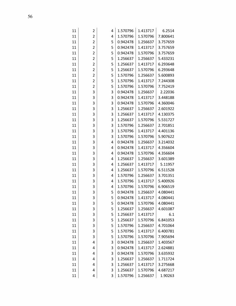
APPENDIX B: INSCRIBED RADII DATA
Appendix B shows the calculated inscribed radius for each set of hypothetical physical
parameters.
Table B.1: Inscribed Radii from MATLAB Simulation
a b c <=>? @=>? r
8 2 3 0.942478 1.256637 2.570992
8 2 3 0.942478 1.413717 3.059412
8 2 3 0.942478 1.570796 3.059412
8 2 3 1.256637 1.256637 2.886174
8 2 3 1.256637 1.413717 3.962323
8 2 3 1.256637 1.570796 4.972927
8 2 3 1.570796 1.256637 3.001666
8 2 3 1.570796 1.413717 4.20119
8 2 3 1.570796 1.570796 5.300943
8 2 4 0.942478 1.256637 2.720294
8 2 4 0.942478 1.413717 2.720294
8 2 4 0.942478 1.570796 2.720294
8 2 4 1.256637 1.256637 3.863936
8 2 4 1.256637 1.413717 4.640043
8 2 4 1.256637 1.570796 4.640043
8 2 4 1.570796 1.256637 4.00125
8 2 4 1.570796 1.413717 5.200961
8 2 4 1.570796 1.570796 5.755867
8 2 5 0.942478 1.256637 2.202272
8 2 5 0.942478 1.413717 2.202272
8 2 5 0.942478 1.570796 2.202272
8 2 5 1.256637 1.256637 3.894868
8 2 5 1.256637 1.413717 3.894868
8 2 5 1.256637 1.570796 3.894868
8 2 5 1.570796 1.256637 4.767599
8 2 5 1.570796 1.413717 4.767599
8 2 5 1.570796 1.570796 4.767599
8 3 3 0.942478 1.256637 1.726268
8 3 3 0.942478 1.413717 2.594224
8 3 3 0.942478 1.570796 3.2
8 3 3 1.256637 1.256637 2.002498
8 3 3 1.256637 1.413717 3.114482
8 3 3 1.256637 1.570796 4.123106
8 3 3 1.570796 1.256637 2.10238

51
8 3 3 1.570796 1.413717 3.301515
8 3 3 1.570796 1.570796 4.410215
8 3 4 0.942478 1.256637 2.716616
8 3 4 0.942478 1.413717 3.008322
8 3 4 0.942478 1.570796 3.008322
8 3 4 1.256637 1.256637 3.001666
8 3 4 1.256637 1.413717 4.1
8 3 4 1.256637 1.570796 5.096077
8 3 4 1.570796 1.256637 3.101612
8 3 4 1.570796 1.413717 4.301163
8 3 4 1.570796 1.570796 5.408327
8 3 5 0.942478 1.256637 2.640076
8 3 5 0.942478 1.413717 2.640076
8 3 5 0.942478 1.570796 2.640076
8 3 5 1.256637 1.256637 4.00125
8 3 5 1.256637 1.413717 4.545327
8 3 5 1.256637 1.570796 4.545327
8 3 5 1.570796 1.256637 4.101219
8 3 5 1.570796 1.413717 5.300943
8 3 5 1.570796 1.570796 5.600893
8 4 3 0.942478 1.256637 0.894427
8 4 3 0.942478 1.413717 1.772005
8 4 3 0.942478 1.570796 2.505993
8 4 3 1.256637 1.256637 1.140175
8 4 3 1.256637 1.413717 2.256103
8 4 3 1.256637 1.570796 3.298485
8 4 3 1.570796 1.256637 1.204159
8 4 3 1.570796 1.413717 2.433105
8 4 3 1.570796 1.570796 3.601389
8 4 4 0.942478 1.256637 1.843909
8 4 4 0.942478 1.413717 2.720294
8 4 4 0.942478 1.570796 3.2
8 4 4 1.256637 1.256637 2.12132
8 4 4 1.256637 1.413717 3.238827
8 4 4 1.256637 1.570796 4.272002
8 4 4 1.570796 1.256637 2.202272
8 4 4 1.570796 1.413717 3.423449
8 4 4 1.570796 1.570796 4.601087
8 4 5 0.942478 1.256637 2.828427
8 4 5 0.942478 1.413717 2.973214
8 4 5 0.942478 1.570796 2.973214
8 4 5 1.256637 1.256637 3.114482
8 4 5 1.256637 1.413717 4.229657
8 4 5 1.256637 1.570796 5.077401
8 4 5 1.570796 1.256637 3.201562

52
8 4 5 1.570796 1.413717 4.418144
8 4 5 1.570796 1.570796 5.600893
9 2 3 0.942478 1.256637 2.745906
9 2 3 0.942478 1.413717 3.569314
9 2 3 0.942478 1.570796 3.569314
9 2 3 1.256637 1.256637 3.080584
9 2 3 1.256637 1.413717 4.310452
9 2 3 1.256637 1.570796 5.434151
9 2 3 1.570796 1.256637 3.201562
9 2 3 1.570796 1.413717 4.501111
9 2 3 1.570796 1.570796 5.800862
9 2 4 0.942478 1.256637 3.257299
9 2 4 0.942478 1.413717 3.257299
9 2 4 0.942478 1.570796 3.257299
9 2 4 1.256637 1.256637 4.060788
9 2 4 1.256637 1.413717 5.295281
9 2 4 1.256637 1.570796 5.403702
9 2 4 1.570796 1.256637 4.20119
9 2 4 1.570796 1.413717 5.500909
9 2 4 1.570796 1.570796 6.747592
9 2 5 0.942478 1.256637 2.778489
9 2 5 0.942478 1.413717 2.778489
9 2 5 0.942478 1.570796 2.778489
9 2 5 1.256637 1.256637 4.701064
9 2 5 1.256637 1.413717 4.701064
9 2 5 1.256637 1.570796 4.701064
9 2 5 1.570796 1.256637 5.200961
9 2 5 1.570796 1.413717 5.755867
9 2 5 1.570796 1.570796 5.755867
9 3 3 0.942478 1.256637 1.90263
9 3 3 0.942478 1.413717 2.906888
9 3 3 0.942478 1.570796 3.640055
9 3 3 1.256637 1.256637 2.202272
9 3 3 1.256637 1.413717 3.452535
9 3 3 1.256637 1.570796 4.609772
9 3 3 1.570796 1.256637 2.302173
9 3 3 1.570796 1.413717 3.701351
9 3 3 1.570796 1.570796 4.909175
9 3 4 0.942478 1.256637 2.886174
9 3 4 0.942478 1.413717 3.535534
9 3 4 0.942478 1.570796 3.535534
9 3 4 1.256637 1.256637 3.201562
9 3 4 1.256637 1.413717 4.440721
9 3 4 1.256637 1.570796 5.565968
9 3 4 1.570796 1.256637 3.301515

53
9 3 4 1.570796 1.413717 4.701064
9 3 4 1.570796 1.570796 5.907622
9 3 5 0.942478 1.256637 3.195309
9 3 5 0.942478 1.413717 3.195309
9 3 5 0.942478 1.570796 3.195309
9 3 5 1.256637 1.256637 4.20119
9 3 5 1.256637 1.413717 5.315073
9 3 5 1.256637 1.570796 5.315073
9 3 5 1.570796 1.256637 4.301163
9 3 5 1.570796 1.413717 5.700877
9 3 5 1.570796 1.570796 6.600758
9 4 3 0.942478 1.256637 1.077033
9 4 3 0.942478 1.413717 2.088061
9 4 3 0.942478 1.570796 2.906888
9 4 3 1.256637 1.256637 1.334166
9 4 3 1.256637 1.413717 2.601922
9 4 3 1.256637 1.570796 3.764306
9 4 3 1.570796 1.256637 1.50333
9 4 3 1.570796 1.413717 2.801785
9 4 3 1.570796 1.570796 4.101219
9 4 4 0.942478 1.256637 2.039608
9 4 4 0.942478 1.413717 3.036445
9 4 4 0.942478 1.570796 3.7
9 4 4 1.256637 1.256637 2.319483
9 4 4 1.256637 1.413717 3.590265
9 4 4 1.256637 1.570796 4.729693
9 4 4 1.570796 1.256637 2.501999
9 4 4 1.570796 1.413717 3.801316
9 4 4 1.570796 1.570796 5.10098
9 4 5 0.942478 1.256637 3.026549
9 4 5 0.942478 1.413717 3.49285
9 4 5 0.942478 1.570796 3.49285
9 4 5 1.256637 1.256637 3.313608
9 4 5 1.256637 1.413717 4.570558
9 4 5 1.256637 1.570796 5.700877
9 4 5 1.570796 1.256637 3.49285
9 4 5 1.570796 1.413717 4.801042
9 4 5 1.570796 1.570796 6.10082
10 2 3 0.942478 1.256637 2.915476
10 2 3 0.942478 1.413717 3.981206
10 2 3 0.942478 1.570796 3.981206
10 2 3 1.256637 1.256637 3.255764
10 2 3 1.256637 1.413717 4.638965
10 2 3 1.256637 1.570796 5.913544
10 2 3 1.570796 1.256637 3.40147

54
10 2 3 1.570796 1.413717 4.90102
10 2 3 1.570796 1.570796 6.300794
10 2 4 0.942478 1.256637 3.7
10 2 4 0.942478 1.413717 3.7
10 2 4 0.942478 1.570796 3.7
10 2 4 1.256637 1.256637 4.242641
10 2 4 1.256637 1.413717 5.632051
10 2 4 1.256637 1.570796 6.161169
10 2 4 1.570796 1.256637 4.401136
10 2 4 1.570796 1.413717 5.900847
10 2 4 1.570796 1.570796 7.300685
10 2 5 0.942478 1.256637 3.264966
10 2 5 0.942478 1.413717 3.264966
10 2 5 0.942478 1.570796 3.264966
10 2 5 1.256637 1.256637 5.234501
10 2 5 1.256637 1.413717 5.515433
10 2 5 1.256637 1.570796 5.515433
10 2 5 1.570796 1.256637 5.400926
10 2 5 1.570796 1.413717 6.747592
10 2 5 1.570796 1.570796 6.747592
10 3 3 0.942478 1.256637 2.061553
10 3 3 0.942478 1.413717 3.162278
10 3 3 0.942478 1.570796 4
10 3 3 1.256637 1.256637 2.402082
10 3 3 1.256637 1.413717 3.801316
10 3 3 1.256637 1.570796 5.069517
10 3 3 1.570796 1.256637 2.501999
10 3 3 1.570796 1.413717 4.00125
10 3 3 1.570796 1.570796 5.408327
10 3 4 0.942478 1.256637 3.041381
10 3 4 0.942478 1.413717 3.945884
10 3 4 0.942478 1.570796 3.945884
10 3 4 1.256637 1.256637 3.40147
10 3 4 1.256637 1.413717 4.785394
10 3 4 1.256637 1.570796 6.041523
10 3 4 1.570796 1.256637 3.501428
10 3 4 1.570796 1.413717 5.001
10 3 4 1.570796 1.570796 6.407027
10 3 5 0.942478 1.256637 3.640055
10 3 5 0.942478 1.413717 3.640055
10 3 5 0.942478 1.570796 3.640055
10 3 5 1.256637 1.256637 4.401136
10 3 5 1.256637 1.413717 5.770615
10 3 5 1.256637 1.570796 6.080296
10 3 5 1.570796 1.256637 4.501111

55
10 3 5 1.570796 1.413717 6.000833
10 3 5 1.570796 1.570796 7.406079
10 4 3 0.942478 1.256637 1.204159
10 4 3 0.942478 1.413717 2.34094
10 4 3 0.942478 1.570796 3.264966
10 4 3 1.256637 1.256637 1.513275
10 4 3 1.256637 1.413717 2.927456
10 4 3 1.256637 1.570796 4.22019
10 4 3 1.570796 1.256637 1.702939
10 4 3 1.570796 1.413717 3.201562
10 4 3 1.570796 1.570796 4.601087
10 4 4 0.942478 1.256637 2.202272
10 4 4 0.942478 1.413717 3.289377
10 4 4 0.942478 1.570796 4.1
10 4 4 1.256637 1.256637 2.507987
10 4 4 1.256637 1.413717 3.920459
10 4 4 1.256637 1.570796 5.197115
10 4 4 1.570796 1.256637 2.701851
10 4 4 1.570796 1.413717 4.20119
10 4 4 1.570796 1.570796 5.600893
10 4 5 0.942478 1.256637 3.17805
10 4 5 0.942478 1.413717 3.905125
10 4 5 0.942478 1.570796 3.905125
10 4 5 1.256637 1.256637 3.50571
10 4 5 1.256637 1.413717 4.916299
10 4 5 1.256637 1.570796 6.168468
10 4 5 1.570796 1.256637 3.701351
10 4 5 1.570796 1.413717 5.200961
10 4 5 1.570796 1.570796 6.600758
11 2 3 0.942478 1.256637 3.080584
11 2 3 0.942478 1.413717 4.254409
11 2 3 0.942478 1.570796 4.393177
11 2 3 1.256637 1.256637 3.452535
11 2 3 1.256637 1.413717 4.981967
11 2 3 1.256637 1.570796 6.378871
11 2 3 1.570796 1.256637 3.601389
11 2 3 1.570796 1.413717 5.261179
11 2 3 1.570796 1.570796 6.800735
11 2 4 0.942478 1.256637 4.060788
11 2 4 0.942478 1.413717 4.123106
11 2 4 0.942478 1.570796 4.123106
11 2 4 1.256637 1.256637 4.440721
11 2 4 1.256637 1.413717 5.968249
11 2 4 1.256637 1.570796 6.92026
11 2 4 1.570796 1.256637 4.601087
56
11 2 4 1.570796 1.413717 6.2514
11 2 4 1.570796 1.570796 7.800641
11 2 5 0.942478 1.256637 3.757659
11 2 5 0.942478 1.413717 3.757659
11 2 5 0.942478 1.570796 3.757659
11 2 5 1.256637 1.256637 5.433231
11 2 5 1.256637 1.413717 6.293648
11 2 5 1.256637 1.570796 6.293648
11 2 5 1.570796 1.256637 5.600893
11 2 5 1.570796 1.413717 7.244308
11 2 5 1.570796 1.570796 7.752419
11 3 3 0.942478 1.256637 2.22036
11 3 3 0.942478 1.413717 3.448188
11 3 3 0.942478 1.570796 4.360046
11 3 3 1.256637 1.256637 2.601922
11 3 3 1.256637 1.413717 4.130375
11 3 3 1.256637 1.570796 5.531727
11 3 3 1.570796 1.256637 2.701851
11 3 3 1.570796 1.413717 4.401136
11 3 3 1.570796 1.570796 5.907622
11 3 4 0.942478 1.256637 3.214032
11 3 4 0.942478 1.413717 4.356604
11 3 4 0.942478 1.570796 4.356604
11 3 4 1.256637 1.256637 3.601389
11 3 4 1.256637 1.413717 5.11957
11 3 4 1.256637 1.570796 6.511528
11 3 4 1.570796 1.256637 3.701351
11 3 4 1.570796 1.413717 5.400926
11 3 4 1.570796 1.570796 6.906519
11 3 5 0.942478 1.256637 4.080441
11 3 5 0.942478 1.413717 4.080441
11 3 5 0.942478 1.570796 4.080441
11 3 5 1.256637 1.256637 4.601087
11 3 5 1.256637 1.413717 6.1
11 3 5 1.256637 1.570796 6.841053
11 3 5 1.570796 1.256637 4.701064
11 3 5 1.570796 1.413717 6.400781
11 3 5 1.570796 1.570796 7.905694
11 4 3 0.942478 1.256637 1.403567
11 4 3 0.942478 1.413717 2.624881
11 4 3 0.942478 1.570796 3.635932
11 4 3 1.256637 1.256637 1.711724
11 4 3 1.256637 1.413717 3.275668
11 4 3 1.256637 1.570796 4.687217
11 4 3 1.570796 1.256637 1.90263

57
11 4 3 1.570796 1.413717 3.501428
11 4 3 1.570796 1.570796 5.10098
11 4 4 0.942478 1.256637 2.376973
11 4 4 0.942478 1.413717 3.573514
11 4 4 0.942478 1.570796 4.465423
11 4 4 1.256637 1.256637 2.707397
11 4 4 1.256637 1.413717 4.257934
11 4 4 1.256637 1.570796 5.67186
11 4 4 1.570796 1.256637 2.901724
11 4 4 1.570796 1.413717 4.501111
11 4 4 1.570796 1.570796 6.10082
11 4 5 0.942478 1.256637 3.354102
11 4 5 0.942478 1.413717 4.341659
11 4 5 0.942478 1.570796 4.341659
11 4 5 1.256637 1.256637 3.705401
11 4 5 1.256637 1.413717 5.246904
11 4 5 1.256637 1.570796 6.640783
11 4 5 1.570796 1.256637 3.901282
11 4 5 1.570796 1.413717 5.500909
11 4 5 1.570796 1.570796 7.100704
12 2 3 0.942478 1.256637 3.238827
12 2 3 0.942478 1.413717 4.531004
12 2 3 0.942478 1.570796 4.805206
12 2 3 1.256637 1.256637 3.634556
12 2 3 1.256637 1.413717 5.315073
12 2 3 1.256637 1.570796 6.824954
12 2 3 1.570796 1.256637 3.801316
12 2 3 1.570796 1.413717 5.600893
12 2 3 1.570796 1.570796 7.300685
12 2 4 0.942478 1.256637 4.229657
12 2 4 0.942478 1.413717 4.554119
12 2 4 0.942478 1.570796 4.554119
12 2 4 1.256637 1.256637 4.627094
12 2 4 1.256637 1.413717 6.296825
12 2 4 1.256637 1.570796 7.580237
12 2 4 1.570796 1.256637 4.801042
12 2 4 1.570796 1.413717 6.600758
12 2 4 1.570796 1.570796 8.300602
12 2 5 0.942478 1.256637 4.204759
12 2 5 0.942478 1.413717 4.204759
12 2 5 0.942478 1.570796 4.204759
12 2 5 1.256637 1.256637 5.622277
12 2 5 1.256637 1.413717 7
12 2 5 1.256637 1.570796 7
12 2 5 1.570796 1.256637 5.800862

58
12 2 5 1.570796 1.413717 7.600658
12 2 5 1.570796 1.570796 8.746428
12 3 3 0.942478 1.256637 2.402082
12 3 3 0.942478 1.413717 3.733631
12 3 3 0.942478 1.570796 4.720169
12 3 3 1.256637 1.256637 2.801785
12 3 3 1.256637 1.413717 4.455334
12 3 3 1.256637 1.570796 5.990826
12 3 3 1.570796 1.256637 2.901724
12 3 3 1.570796 1.413717 4.716991
12 3 3 1.570796 1.570796 6.412488
12 3 4 0.942478 1.256637 3.373426
12 3 4 0.942478 1.413717 4.661545
12 3 4 0.942478 1.570796 4.767599
12 3 4 1.256637 1.256637 3.801316
12 3 4 1.256637 1.413717 5.445181
12 3 4 1.256637 1.570796 6.957011
12 3 4 1.570796 1.256637 3.901282
12 3 4 1.570796 1.413717 5.714018
12 3 4 1.570796 1.570796 7.410803
12 3 5 0.942478 1.256637 4.356604
12 3 5 0.942478 1.413717 4.522168
12 3 5 0.942478 1.570796 4.522168
12 3 5 1.256637 1.256637 4.785394
12 3 5 1.256637 1.413717 6.432729
12 3 5 1.256637 1.570796 7.516648
12 3 5 1.570796 1.256637 4.90102
12 3 5 1.570796 1.413717 6.71193
12 3 5 1.570796 1.570796 8.409518
12 4 3 0.942478 1.256637 1.529706
12 4 3 0.942478 1.413717 2.912044
12 4 3 0.942478 1.570796 3.996248
12 4 3 1.256637 1.256637 1.90263
12 4 3 1.256637 1.413717 3.605551
12 4 3 1.256637 1.570796 5.141984
12 4 3 1.570796 1.256637 2.10238
12 4 3 1.570796 1.413717 3.901282
12 4 3 1.570796 1.570796 5.600893
12 4 4 0.942478 1.256637 2.517936
12 4 4 0.942478 1.413717 3.848376
12 4 4 0.942478 1.570796 4.825971
12 4 4 1.256637 1.256637 2.901724
12 4 4 1.256637 1.413717 4.589118
12 4 4 1.256637 1.570796 6.113101
12 4 4 1.570796 1.256637 3.101612

59
12 4 4 1.570796 1.413717 4.90102
12 4 4 1.570796 1.570796 6.600758
12 4 5 0.942478 1.256637 3.512834
12 4 5 0.942478 1.413717 4.751842
12 4 5 0.942478 1.570796 4.751842
12 4 5 1.256637 1.256637 3.901282
12 4 5 1.256637 1.413717 5.57315
12 4 5 1.256637 1.570796 7.083078
12 4 5 1.570796 1.256637 4.101219
12 4 5 1.570796 1.413717 5.900847
12 4 5 1.570796 1.570796 7.600658

60
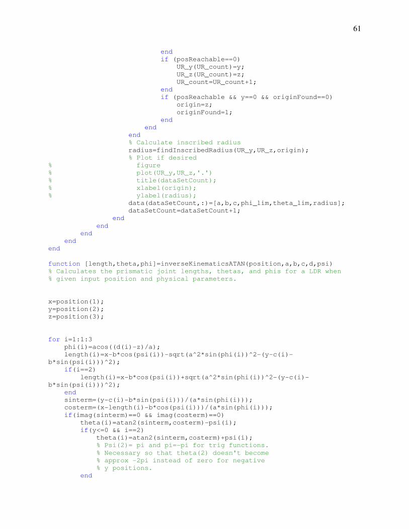
APPENDIX C: INSCRIBED RADII SIMULATION CODE
Appendix C shows the MATLAB script used to calculate the inscribed radii.
% This program calculates the inscribed radius for numerous
% LDRs of varying parameters
% Prepare workspace
clear all
close all
% Set constants
x=20;
psi=[pi/3,pi,-pi/3];
d=[-1,-1,-1];
% Set empty variables
L=[0,0,0];
phi=[0,0,0];
theta=[0,0,0];
origin=-1;
% Set up data storage
data=zeros(5*3^4,6);
dataSetCount=1;
% Set up flags
posReachable=0;
UR_count=1;
originFound=0;
% Loop through parameters
for a=8:1:12
for b=2:1:4
for c=3:1:5
for phi_lim=0.3*pi:0.1*pi:0.5*pi
for theta_lim=0.4*pi:0.05*pi:0.5*pi
UR_count=1;
origin=-1;
originFound=0;
for y= -20:0.1:20
for z= -1:-0.1:-14
posReachable=1;
testPos=[x,y,z];
[L,theta,phi]=inverseKinematicsATAN(testPos,a,b,[-c,0,c],d,psi);
if((max(imag([L,theta,phi])))~=0)
posReachable=0;
end
if(max(abs(theta))>theta_lim)
posReachable=0;
end
if(max(abs(phi))>phi_lim)
posReachable=0;
61
end
if (posReachable==0)
UR_y(UR_count)=y;
UR_z(UR_count)=z;
UR_count=UR_count+1;
end
if (posReachable && y==0 && originFound==0)
origin=z;
originFound=1;
end
end
end
% Calculate inscribed radius
radius=findInscribedRadius(UR_y,UR_z,origin);
% Plot if desired
% figure
% plot(UR_y,UR_z,'.')
% title(dataSetCount);
% xlabel(origin);
% ylabel(radius);
data(dataSetCount,:)=[a,b,c,phi_lim,theta_lim,radius];
dataSetCount=dataSetCount+1;
end
end
end
end
end
function [length,theta,phi]=inverseKinematicsATAN(position,a,b,c,d,psi)
% Calculates the prismatic joint lengths, thetas, and phis for a LDR when
% given input position and physical parameters.
x=position(1);
y=position(2);
z=position(3);
for i=1:1:3
phi(i)=acos((d(i)-z)/a);
length(i)=x-b*cos(psi(i))-sqrt(a^2*sin(phi(i))^2-(y-c(i)-
b*sin(psi(i)))^2);
if(i==2)
length(i)=x-b*cos(psi(i))+sqrt(a^2*sin(phi(i))^2-(y-c(i)-
b*sin(psi(i)))^2);
end
sinterm=(y-c(i)-b*sin(psi(i)))/(a*sin(phi(i)));
costerm=(x-length(i)-b*cos(psi(i)))/(a*sin(phi(i)));
if(imag(sinterm)==0 && imag(costerm)==0)
theta(i)=atan2(sinterm,costerm)-psi(i);
if(y<=0 && i==2)
theta(i)=atan2(sinterm,costerm)+psi(i);
% Psi(2)= pi and pi=-pi for trig functions.
% Necessary so that theta(2) doesn't become
% approx -2pi instead of zero for negative
% y positions.
end

62
else
theta(i)=10+10*i;
% Set theta as a large complex number if out of bounds.
end
end
end
% Finds the max radius when given an array of points
% that CANNOT be reached. Also requires an origin
% z position to calculate distance.
function radius=findInscribedRadius(y,z,origin)
numPoints=length(y);
radius=10000;
currentRadius=0;
for i=1:numPoints
if (z(i)<origin)
currentRadius=sqrt((z(i)-origin)^2+(y(i))^2);
if(currentRadius<radius)
radius=currentRadius;
end
end
end

63
APPENDIX D: PHYSICAL LDR CODE
Appendix D shows the Arduino code used on the constructed Linear Delta Robot.
// A program to control the constructed LDR
// Include libraries
#include <math.h>
#include <EEPROM.h>
#include <Wire.h>
#include <Adafruit_MotorShield.h>
#include "utility/Adafruit_PWMServoDriver.h"
#include <LinearDeltaCom.h>
#include <AccelStepper.h>
// Add all the #defines and global variables that would be class variables here
////////////////////////////////////////////////////////////////////
// Constants
////////////////////////////////////////////////////////////////////
// Memory Constants
#define EEPROM_ADDRESS_BACK_TICKS_START 0x0018
#define EEPROM_ADDRESS_MID_TICKS_START 0x0020
#define EEPROM_ADDRESS_FRONT_TICKS_START 0x0028
// Define default physical parameters
#define DEFAULT_a 9.25
#define DEFAULT_b 3
#define DEFAULT_c1 -3.5
#define DEFAULT_c2 0
#define DEFAULT_c3 3.5
#define DEFAULT_d1 -2.656
#define DEFAULT_d2 -2.656
#define DEFAULT_d3 -2.656
#define DEFAULT_psi1 1.04719
#define DEFAULT_psi2 3.14159
#define DEFAULT_psi3 -1.04719
#define DEFAULT_ticksPerRev 200
#define DEFAULT_threadsPerInch 10
// Define I/O Assignments
#define L1_switch_pin 2
#define L2_switch_pin 3
#define L3_switch_pin 4
////////////////////////////////////////////////////////////////////
// Variables
////////////////////////////////////////////////////////////////////
// Physical parameters
float a;
float b;
float c1;
float c2;
float c3;
float d1;
float d2;
float d3;
float psi1;
float psi2;
float psi3;
long ticksPerRev;
long threadsPerInch;
float currentPosition[3];
long currentTicks[3];
Adafruit_MotorShield AFMSbot(0x60);

64
Adafruit_MotorShield AFMStop(0x61);
Adafruit_StepperMotor *frontStepper = AFMStop.getStepper(200, 2);
Adafruit_StepperMotor *midStepper = AFMSbot.getStepper(200, 1);
Adafruit_StepperMotor *backStepper = AFMStop.getStepper(200, 1);
LinearDeltaCom deltaCom;
AccelStepper stepperFront(forwardstep1, backwardstep1);
AccelStepper stepperMid(forwardstep2, backwardstep2);
AccelStepper stepperBack(forwardstep3, backwardstep3);
void setup(){
AFMSbot.begin();
AFMStop.begin();
setDefaultParams();
loadEEPROM();
Serial.begin(115200);
delay(1000);
deltaCom.registerMoveCallback(movePos);
deltaCom.registerXMoveCallback(xMove);
deltaCom.registerYMoveCallback(yMove);
deltaCom.registerZMoveCallback(zMove);
deltaCom.registerHomeCallback(resetLengths);
deltaCom.registerRequestPositionCallback(sendPositionData);
}
void loop(){
stepperFront.run();
stepperMid.run();
stepperBack.run();
}
////////////////////////////////////////////////////////////////////
// Setup Functions
////////////////////////////////////////////////////////////////////
void setDefaultParams(){
a=DEFAULT_a;
b=DEFAULT_b;
c1=DEFAULT_c1;
c2=DEFAULT_c2;
c3=DEFAULT_c3;
d1=DEFAULT_d1;
d2=DEFAULT_d2;
d3=DEFAULT_d3;
psi1=DEFAULT_psi1;
psi2=DEFAULT_psi2;
psi3=DEFAULT_psi3;
ticksPerRev=DEFAULT_ticksPerRev;
threadsPerInch=DEFAULT_threadsPerInch;
pinMode(L1_switch_pin,INPUT_PULLUP);
pinMode(L2_switch_pin,INPUT_PULLUP);
pinMode(L3_switch_pin,INPUT_PULLUP);
stepperFront.setAcceleration(100);
stepperMid.setAcceleration(100);
stepperBack.setAcceleration(100);
stepperFront.setMaxSpeed(600);
stepperMid.setMaxSpeed(600);
stepperBack.setMaxSpeed(600);
}
// AccelStepper functions
void forwardstep1() {
frontStepper->onestep(FORWARD, SINGLE);
}
void backwardstep1() {
frontStepper->onestep(BACKWARD, SINGLE);
}
void forwardstep2() {

65
midStepper->onestep(FORWARD, SINGLE);
}
void backwardstep2() {
midStepper->onestep(BACKWARD, SINGLE);
}
void forwardstep3() {
backStepper->onestep(FORWARD, SINGLE);
}
void backwardstep3() {
backStepper->onestep(BACKWARD, SINGLE);
}
void serialEvent(){
while(Serial.available()){
deltaCom.handleRxByte(Serial.read());
}
}
////////////////////////////////////////////////////////////////////
// Movement Functions
////////////////////////////////////////////////////////////////////
void movePos(float targetX, float targetY, float targetZ){
Serial.print("Order received: Move");
Serial.print("\n");
//Calculate lengths
int positionReachable=1;
float targetPosition[]={
targetX,targetY,targetZ };
float finalLengths[3];
long finalTicks[3];
long deltaTicks[3];
inverseKinematics(targetPosition,finalLengths);
for (int i=0; i <3; i++){
if((finalLengths[i]<1.75) || (finalLengths[i]>15.25)){
positionReachable=0;
Serial.println();
Serial.print("Position Unreachable!");
Serial.println();
}
}
for(int i=0; i < 3; i++){
finalTicks[i]=length2ticks(finalLengths[i]);
deltaTicks[i]=finalTicks[i]-currentTicks[i];
}
// Make the move
if(positionReachable==1){
stepperFront.move(deltaTicks[0]);
stepperMid.move(deltaTicks[1]);
stepperBack.move(deltaTicks[2]);
// Update position
for (int i=0; i < 3; i++){
currentPosition[i]=targetPosition[i];
currentTicks[i]=finalTicks[i];
}
}
updateEEPROM();
}
void xMove(float deltaX){
Serial.print("Order received: MoveX");
Serial.print("\n");
float targetPosition[3]={
currentPosition[0],currentPosition[1],currentPosition[2] };
targetPosition[0]=targetPosition[0]+deltaX;
movePos(targetPosition[0],targetPosition[1],targetPosition[2]);
}
void yMove(float deltaY){
Serial.print("Order received: MoveY");

66
Serial.print("\n");
float targetPosition[3]={
currentPosition[0],currentPosition[1],currentPosition[2] };
targetPosition[1]=targetPosition[1]+deltaY;
movePos(targetPosition[0],targetPosition[1],targetPosition[2]);
}
void zMove(float deltaZ){
Serial.print("Order received: MoveZ");
Serial.print("\n");
float targetPosition[3]={
currentPosition[0],currentPosition[1],currentPosition[2] };
targetPosition[2]=targetPosition[2]+deltaZ;
movePos(targetPosition[0],targetPosition[1],targetPosition[2]);
}
void moveHome(){
float homePos[]={
8,0,-11 };
movePos(homePos[0],homePos[1],homePos[2]);
}
void resetLengths(){
Serial.print("Order received: ReHome");
Serial.print("\n");
while(!(digitalRead(L1_switch_pin)&&digitalRead(L2_switch_pin)&&digitalRead(L3_switch_pin))){
if(digitalRead(L1_switch_pin)==0){
stepperFront.move(-1);
}
else {
stepperFront.move(0);
}
if(digitalRead(L2_switch_pin)==0){
stepperMid.move(1);
}
else {
stepperMid.move(0);
}
if(digitalRead(L3_switch_pin)==0){
stepperBack.move(-1);
}
else {
stepperBack.move(0);
}
stepperFront.run();
stepperMid.run();
stepperBack.run();
}
currentTicks[0]=3813;
currentTicks[1]=30438;
currentTicks[2]=3938;
moveHome();
}
////////////////////////////////////////////////////////////////////
// Memory Functions
////////////////////////////////////////////////////////////////////
void loadEEPROM(){
// Ticks
currentTicks[0]=256*(unsigned long) EEPROM.read(EEPROM_ADDRESS_BACK_TICKS_START)+ (unsigned long)
EEPROM.read(EEPROM_ADDRESS_BACK_TICKS_START+1);
currentTicks[1]=256*(unsigned long) EEPROM.read(EEPROM_ADDRESS_MID_TICKS_START)+(unsigned long)
EEPROM.read(EEPROM_ADDRESS_MID_TICKS_START+1);
currentTicks[2]=256*(unsigned long) EEPROM.read(EEPROM_ADDRESS_FRONT_TICKS_START)+(unsigned long)
EEPROM.read(EEPROM_ADDRESS_FRONT_TICKS_START+1);
}
void updateEEPROM(){

67
// Ticks
EEPROM.write(EEPROM_ADDRESS_BACK_TICKS_START, currentTicks[0]/256);
EEPROM.write(EEPROM_ADDRESS_BACK_TICKS_START+1, currentTicks[0]%256);
EEPROM.write(EEPROM_ADDRESS_MID_TICKS_START, currentTicks[1]/256);
EEPROM.write(EEPROM_ADDRESS_MID_TICKS_START+1, currentTicks[1]%256);
EEPROM.write(EEPROM_ADDRESS_FRONT_TICKS_START, currentTicks[2]/256);
EEPROM.write(EEPROM_ADDRESS_FRONT_TICKS_START+1, currentTicks[2]%256);
}
////////////////////////////////////////////////////////////////////
// Helper Functions
////////////////////////////////////////////////////////////////////
long length2ticks(float length){
long ticks=length*ticksPerRev*threadsPerInch;
return ticks;
}
float ticks2length(float ticks){
float length=ticks/ticksPerRev/threadsPerInch;
return length;
}
void inverseKinematics(float targetPosition[], float lengths[]){
float x=targetPosition[0];
float y=targetPosition[1];
float z=targetPosition[2];
float t1=a*a-d1*d1+2*d1*z-z*z;
float t2=a*a-d2*d2+2*d2*z-z*z;
float t3=a*a-d3*d3+2*d3*z-z*z;
float L1=x-b*cos(psi1)-sqrt(1/t1*(t1-sin(psi1)*sin(psi1)*b*b-2*sin(psi1)*b*c1+2*sin(psi1)*b*y-c1*c1+2*c1*y-y*y))*sqrt(t1);
float L2=x-b*cos(psi2)+sqrt(1/t2*(t2-sin(psi2)*sin(psi2)*b*b-2*sin(psi2)*b*c2+2*sin(psi2)*b*y-c2*c2+2*c2*y-y*y))*sqrt(t2);
float L3=x-b*cos(psi3)-sqrt(1/t3*(t3-sin(psi3)*sin(psi3)*b*b-2*sin(psi3)*b*c3+2*sin(psi3)*b*y-c3*c3+2*c3*y-y*y))*sqrt(t3);
lengths[0]=L1;
lengths[1]=L2;
lengths[2]=L3;
}
void sendPositionData(){
Serial.println();
Serial.print("Position Request Received");
Serial.println("");
Serial.print(" x=");
Serial.print(currentPosition[0]);
Serial.print(" y=");
Serial.print(currentPosition[1]);
Serial.print(" z=");
Serial.print(currentPosition[2]);
Serial.println("");
Serial.print("J1 ticks=");
Serial.print(currentTicks[0]);
Serial.println("");
Serial.print("J2 ticks=");
Serial.print(currentTicks[1]);
Serial.println("");
Serial.print("J3 ticks=");
Serial.print(currentTicks[2]);
Serial.println("");
Serial.print("\n");
}
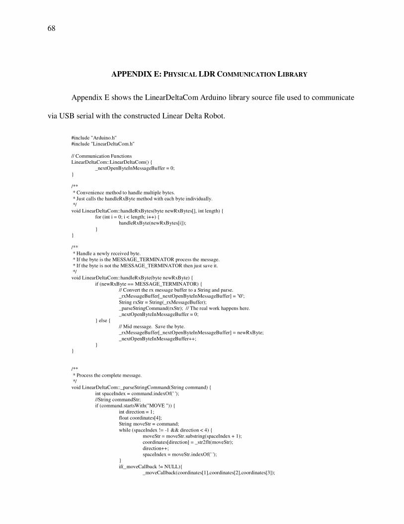
68
APPENDIX E: PHYSICAL LDR COMMUNICATION LIBRARY
Appendix E shows the LinearDeltaCom Arduino library source file used to communicate
via USB serial with the constructed Linear Delta Robot.
#include "Arduino.h"
#include "LinearDeltaCom.h"
// Communication Functions
LinearDeltaCom::LinearDeltaCom() {
_nextOpenByteInMessageBuffer = 0;
}
/**
* Convenience method to handle multiple bytes.
* Just calls the handleRxByte method with each byte individually.
*/
void LinearDeltaCom::handleRxBytes(byte newRxBytes[], int length) {
for (int i = 0; i < length; i++) {
handleRxByte(newRxBytes[i]);
}
}
/**
* Handle a newly received byte.
* If the byte is the MESSAGE_TERMINATOR process the message.
* If the byte is not the MESSAGE_TERMINATOR then just save it.
*/
void LinearDeltaCom::handleRxByte(byte newRxByte) {
if (newRxByte == MESSAGE_TERMINATOR) {
// Convert the rx message buffer to a String and parse.
_rxMessageBuffer[_nextOpenByteInMessageBuffer] = '\0';
String rxStr = String(_rxMessageBuffer);
_parseStringCommand(rxStr); // The real work happens here.
_nextOpenByteInMessageBuffer = 0;
} else {
// Mid message. Save the byte.
_rxMessageBuffer[_nextOpenByteInMessageBuffer] = newRxByte;
_nextOpenByteInMessageBuffer++;
}
}
/**
* Process the complete message.
*/
void LinearDeltaCom::_parseStringCommand(String command) {
int spaceIndex = command.indexOf(' ');
//String commandStr;
if (command.startsWith("MOVE ")) {
int direction = 1;
float coordinates[4];
String moveStr = command;
while (spaceIndex != -1 && direction < 4) {
moveStr = moveStr.substring(spaceIndex + 1);
coordinates[direction] = _str2flt(moveStr);
direction++;
spaceIndex = moveStr.indexOf(' ');
}
if(_moveCallback != NULL){
_moveCallback(coordinates[1],coordinates[2],coordinates[3]);

69
}
} else if (command.startsWith("XMOVE")) {
String xMoveStr = command.substring(spaceIndex + 1);
if (_xMoveCallback != NULL) {
_xMoveCallback(_str2flt(xMoveStr));
}
} else if (command.startsWith("YMOVE")) {
String yMoveStr = command.substring(spaceIndex + 1);
if (_yMoveCallback != NULL) {
_yMoveCallback(_str2flt(yMoveStr));
}
} else if (command.startsWith("ZMOVE")) {
String zMoveStr = command.substring(spaceIndex + 1);
if (_zMoveCallback != NULL) {
_zMoveCallback(_str2flt(zMoveStr));
}
} else if (command.startsWith("SMOOTHMOVE")) {
int smoothDirection = 1;
float smoothCoordinates[4];
String smoothMoveStr = command;
while (spaceIndex != -1 && smoothDirection < 4) {
smoothMoveStr = smoothMoveStr.substring(spaceIndex + 1);
smoothCoordinates[smoothDirection] = _str2flt(smoothMoveStr);
smoothDirection++;
spaceIndex = smoothMoveStr.indexOf(' ');
}
if(_smoothMoveCallback != NULL){
_smoothMoveCallback(smoothCoordinates[1],smoothCoordinates[2],smoothCoordinates[3]);
}
} else if (command.startsWith("SPEED")) {
String speedStr = command.substring(spaceIndex + 1);
if (_setSpeedCallback != NULL) {
_setSpeedCallback(_str2flt(speedStr));
}
} else if (command.startsWith("SMOOTHSPEED")) {
String smoothSpeedStr = command.substring(spaceIndex + 1);
if (_setSmoothSpeedCallback != NULL) {
_setSmoothSpeedCallback(_str2flt(smoothSpeedStr));
}
} else if (command.startsWith("HOME")) {
if (_homeCallback != NULL) {
_homeCallback();
}
} else if (command.startsWith("POSITION")) {
if (_requestPositionCallback != NULL) {
_requestPositionCallback();
}
}
}
// Attach the callbacks
void LinearDeltaCom::registerMoveCallback(
void (*moveCallback)(float x, float y, float z)){
_moveCallback=moveCallback;
}
void LinearDeltaCom::registerXMoveCallback(
void (*xMoveCallback)(float x)){
_xMoveCallback=xMoveCallback;
}
void LinearDeltaCom::registerYMoveCallback(
void (*yMoveCallback)(float y)){
_yMoveCallback=yMoveCallback;
}
void LinearDeltaCom::registerZMoveCallback(
void (*zMoveCallback)(float z)){
_zMoveCallback=zMoveCallback;
}

70
void LinearDeltaCom::registerSmoothMoveCallback(
void (*smoothMoveCallback)(float x, float y, float z)){
_smoothMoveCallback=smoothMoveCallback;
}
void LinearDeltaCom::registerSetSpeedCallback(
void (*setSpeedCallback)(float speed)){
_setSpeedCallback=setSpeedCallback;
}
void LinearDeltaCom::registerSetSmoothSpeedCallback(
void (*setSmoothSpeedCallback)(float smoothSpeed)){
_setSmoothSpeedCallback=setSmoothSpeedCallback;
}
void LinearDeltaCom::registerHomeCallback(
void (*homeCallback)()){
_homeCallback=homeCallback;
}
void LinearDeltaCom::registerRequestPositionCallback(
void (*requestPositionCallback)()){
_requestPositionCallback=requestPositionCallback;
}
// Helper function
float LinearDeltaCom::_str2flt(String inputString){
char charArray[inputString.length()+1];
inputString.toCharArray(charArray,sizeof(charArray));
float outputFloat=atof(charArray);
return outputFloat;
}