Workshop onUbiquitous Data Mining

in conjunction with the23rd. International Joint Conference on Artificial

Intelligence (IJCAI 2013)Beijing, China

August 3 - 9, 2013

Edited by

Joao Gama, Michael May, Nuno Marques,Paulo Cortez and Carlos A. Ferreira

Preface

Ubiquitous Data Mining(UDM) uses Data Mining techniques to extract usefulknowledge from data, namely when its characteristics reflect a World in Movement.The goal of this workshop is to convene researchers (from both academia and in-dustry) who deal with techniques such as: decision rules, decision trees, associationrules, clustering, filtering, learning classifier systems, neural networks, support vec-tor machines, preprocessing, postprocessing, feature selection and visualization tech-niques for UDM of distributed and heterogeneous sources in the form of a continuousstream with mobile and/or embedded devices and related themes.

This is the third workshop in the topic. We received 12 submissions that wereevaluated by 3 members of the Program Committee. The PC recommended accept-ing 8 full papers and 2 Position Papers. We have a diverse set of papers focusingfrom activity recognition, predicting taxis demand, trend mining to more theoreticalaspects of learning model rules from data streams. All papers deal with differentaspects of evolving data and/or distributed data.

We would like to thank all people that make this event possible. First of all,we thank authors that submit their work and the Program Committee for the workin reviewing the papers, and proposing suggestions to improve the works. A finalThanks to the IJCAI Workshop Chairs for all the support.

Joao Gama, Michael May, Nuno Marques, Paulo Cortez and Carlos A. FerreiraProgram Chairs

I

Organization

Program Chairs:Joao Gama, Michael May, Nuno Marques, Paulo Cortez and Carlos A. Ferreira

Organizing Chairs:Manuel F. Santos, Pedro P. Rodrigues and Albert Bifet

Publicity Chair:Carlos A. Ferreira

Organized in the context of the project Knowledge Discovery from Ubiquitous DataStreams (PTDC/EIA-EIA/098355/2008). This workshop is funded by the ERDF -European Regional Development Fund through the COMPETE Programme (oper-ational programme for competitiveness) and by the Portuguese Government Fundsthrough the FCT (Portuguese Foundation for Science and Technology).

Program Committee:

• Albert Bifet, Technical University of Catalonia, Spain

• Alfredo Cuzzocrea, University of Calabria, Italy

• Andre Carvalho, University of Sao Paulo (USP), Brazil

• Antoine Cornuejols, LRI, France

• Carlos A. Ferreira, Institute of Engineering of Porto, Portugal

• Eduardo Spinosa, University of Sao Paulo (USP), Brazil

• Elaine Sousa, University of Sao Paulo, Brazil

• Elena Ikonomovska, University St. Cyril & Methodius, Macedonia

• Ernestina Menasalvas, Technical University of Madrid, Spain

• Florent Masseglia, INRIA, France

• Geoffrey Holmes, University of Waikato, New Zealand

• Hadi Tork, LIAAD-INESC TEC, Portugal

• Jesus Aguilar, University of Pablo Olavide, Spain

• Jiong Yang, Case Western Reserve University, USA

• Joao Gama, University of Porto, Portugal

II

• Joao Gomes, I2R A*Star, Singapure

• Joao Mendes Moreira, University of Porto, Portugal

• Jose Avila, University of Malaga, Spain

• Josep Roure, CMU, USA

• Manuel F. Santos, University of Minho, Portugal

• Mark Last, Ben Gurion University, Israel

• Matjaz Gams, Jozef Stefan Institute, Slovenia

• Michael May, Fraunhofer Bonn, Germany

• Min Wang, IBM, USA

• Miroslav Kubat, University of Miami, USA

• Mohamed Gaber, University of Plymouth, UK

• Myra Spiliopoulou, University of Magdeburg, Germany

• Nuno Marques, University of Nova Lisboa, Portugal

• Paulo Cortez, University of Minho, Portugal

• Pedro P. Rodrigues, University of Porto, Portugal

• Philip Yu, IBM Watson, USA

• Raquel Sebastiao, University of Porto, Portugal

• Rasmus Pederson, Copenhagen Business School, Denmark

• Ricard Gavalda, University of Barcelona, Spain

• Shonali Krishnaswamy, Monash University, Australia

• Xiaoyang S. Wang, University of Vermont, USA

• Ying Yang, Monash University, Australia

III

Table of Contents

Invited Talks

Exploiting Label Relationship in Multi-Label Learning . . . . . . . . . . . . . . . . . . . . . 1Zhi-Hua Zhou

NIM: Scalable Distributed Stream Processing System on MobileNetwork Data . . . . . . . . . . . . . . . . . . . . . . . . . . . . . . . . . . . . . . . . . . . . . . . . . . . . . . . . . . . . . 3Wei Fan

Papers

Predicting Globally and Locally: A Comparison of Methods forVehicle Trajectory Prediction . . . . . . . . . . . . . . . . . . . . . . . . . . . . . . . . . . . . . . . . . . . . . . 5William Groves, Ernesto Nunes and Maria Gini

Learning Model Rules from High-Speed Data Streams . . . . . . . . . . . . . . . . . . . . 10Ezilda Almeida, Carlos A. Ferreira and Joao Gama

On Recommending Urban Hotspots to Find Our Next Passenger . . . . . . . . . .17Luis Moreira-Matias, Ricardo Fernandes, Joao Gama, Michel Ferreira,Joao Mendes-Moreira and Luis Damas

Visual Scenes Clustering Using Variational Incremental Learning ofInfinite Generalized Dirichlet Mixture Models . . . . . . . . . . . . . . . . . . . . . . . . . . . . 24Wentao Fan and Nizar Bouguila

Simultaneous segmentation and recognition of gestures forhuman-machine interaction . . . . . . . . . . . . . . . . . . . . . . . . . . . . . . . . . . . . . . . . . . . . . . 29Harold Vasquez, Luis E. Sucar and Hugo J. Escalante

Cicerone: Design of a Real-Time Area Knowledge-Enhanced VenueRecommender . . . . . . . . . . . . . . . . . . . . . . . . . . . . . . . . . . . . . . . . . . . . . . . . . . . . . . . . . . . . 34Daniel Villatoro, Jordi Aranda, Marc Planaguma, Rafael Gimenezand Marc Torrent-Moreno

Road-quality classification and bump detection with bicycle-mountedsmartphones. . . . . . . . . . . . . . . . . . . . . . . . . . . . . . . . . . . . . . . . . . . . . . . . . . . . . . . . . . . . . .39Marius Hoffmann, Michael Mock and Michael May

Simulating Price Interactions by Mining Multivariate FinancialTime Series . . . . . . . . . . . . . . . . . . . . . . . . . . . . . . . . . . . . . . . . . . . . . . . . . . . . . . . . . . . . . . 44Bruno Silva, Luis Cavique and Nuno Marques

Trend template: mining trends with a semi-formal trend model . . . . . . . . . . . 49Olga Streibel, Lars Wißler, Robert Tolksdorf and Danilo Montesi

Ubiquitous Self-Organizing Maps . . . . . . . . . . . . . . . . . . . . . . . . . . . . . . . . . . . . . . . . . 54Bruno Silva and Nuno Marques

IV

Exploiting Label Relationship in Multi-Label

Learning

Zhi-Hua Zhou

National Key Laboratory for Novel Software Technology,Nanjing University, China

zhouzh@nju.edu.cn

Abstract

In many real data mining tasks, one data object is often associated with multi-ple class labels simultaneously; for example, a document may belong to multipletopics, an image can be tagged with multiple terms, etc. Multi-label learningfocuses on such problems, and it is well accepted that the exploitation of rela-tionship among labels is crucial; actually this is the essential difference betweenmulti-label learning and conventional (single-label) supervised learning.

Most multi-label learning approaches try to capture label relationship andthen apply it to help construct prediction models. Some approaches rely on ex-ternal knowledge resources such as label hierarchies, and some approaches try toexploit label relationship by counting the label co-occurrences in training data.These approaches are effective in many cases; however, in real practice, the ex-ternal label relationship is often unavailable, and generating label relationshipfrom training data and then applying to the same training data for model con-struction will greatly increase the overfitting risk. Moreover, the label relation-ship is usually assumed symmetric, and almost all existing approaches exploitit globally by assuming the label correlation be shared among all instances.

Short Bio

Zhi-Hua Zhou is a professor at Nanjing University. His research interests aremainly in machine learning, data mining, pattern recognition and multimediainformation retrieval. In these areas he has published more than 100 papersin leading international journals or conferences, and holds 12 patents. He isthe recipient of the IEEE CIS Outstanding Early Career Award, the Fok YingTung Young Professorship Award, the Microsoft Young Professorship Award,

1

the National Science & Technology Award for Young Scholars of China, andmany other awards including nine international journal/conference paper orcompetition awards. He is an Associate Editor-in-Chief of ”Chinese ScienceBulletin”, Associate Editor or Editorial Boards member of ”ACM Trans. Intel-ligent Systems and Technology” and twelve other journals. He is the Founderand Steering Committee Chair of ACML, and Steering Committee member ofPAKDD and PRICAI. He is the Chair of the AI&PR Technical Committeeof the China Computer Federation, Chair of the Machine Learning TechnicalCommittee of the China Association of AI, the Vice Chair of the Data MiningTechnical Committee of the IEEE Computational Intelligence Society, and theChair of the IEEE Computer Society Nanjing Chapter. He is a Fellow of theIAPR, Fellow of the IEEE, and Fellow of the IET/IEE.

2

NIM: Scalable Distributed Stream Processing

System on Mobile Network Data

Wei Fan

IBM T.J. Watson Research, Hawthorne, NY, USAweifan@us.ibm.com

Abstract

As a typical example of New Moore’s law, the amount of 3G mobile broad-band (MBB) data has grown from 15 to 20 times in the past two years (30TBto 40TB per day on average for a major city in China), real-time processingand mining of these data are becoming increasingly necessary. The overhead ofstorage and file transfer to HDFS, delay in processing, etc are making offlineanalysis on these datasets obsolete. Analysis of these datasets are non-trivial,examples include mobile personal recommendation, anomaly traffic detection,and network fault diagnosis. In this talk, we describe NIM - Network Intelli-gence Miner. NIM is a scalable and elastic streaming solution that analyzesMBB statistics and traffic patterns in real-time and provides information forreal-time decision making. The accuracy of statistical analysis and patternrecognition of NIM is identical to that of off line analysis, while NIM can pro-cess data at line rate. The design and the unique features (e.g., balanced datagrouping, aging strategy) of NIM will be helpful not only for the network dataanalysis but also for other applications.

Short Bio

Dr. Wei Fan is the associate director of Huawei Noah’s Ark Lab. Prior to join-ing Huawei, he received his PhD in Computer Science from Columbia Universityin 2001 and had been working in IBM T.J. Watson Research since 2000. Hismain research interests and experiences are in various areas of data mining anddatabase systems, such as, stream computing, high performance computing,extremely skewed distribution, cost-sensitive learning, risk analysis, ensemblemethods, easy-to-use nonparametric methods, graph mining, predictive featurediscovery, feature selection, sample selection bias, transfer learning, time series

3

analysis, bioinformatics, social network analysis, novel applications and com-mercial data mining systems. His co-authored paper received ICDM’2006 BestApplication Paper Award, he lead the team that used Random Decision Treeto win 2008 ICDM Data Mining Cup Championship. He received 2010 IBMOutstanding Technical Achievement Award for his contribution to IBM Infos-phere Streams. He is the associate editor of ACM Transaction on KnowledgeDiscovery and Data Mining (TKDD).

4

Predicting Globally and Locally: A Comparison of Methodsfor Vehicle Trajectory Prediction

William Groves, Ernesto Nunes, and Maria GiniDepartment of Computer Science and Engineering, University of Minnesota

{groves, enunes, gini}@cs.umn.edu

AbstractWe propose eigen-based and Markov-based meth-ods to explore the global and local structure ofpatterns in real-world GPS taxi trajectories. Ourprimary goal is to predict the subsequent path ofan in-progress taxi trajectory. The exploration ofglobal and local structure in the data differenti-ates this work from the state-of-the-art literaturein trajectory prediction methods, which mostly fo-cuses on local structures and feature selection. Wepropose four algorithms: a frequency based algo-rithm FreqCount, which we use as a benchmark,two eigen-based (EigenStrat, LapStrat), and aMarkov-based algorithm (MCStrat). Pairwise per-formance analysis on a large real-world data set re-veals that LapStrat is the best performer, followedby MCStrat.

1 IntroductionIn order to discover characteristic patterns in large spatio-temporal data sets, mining algorithms have to take into ac-count spatial relations, such as topology and direction, as wellas temporal relations. The increased use of devices that arecapable of storing driving-related spatio-temporal informa-tion helps researchers and practitioners gather the necessarydata to understand driving patterns in cities, and to designlocation-based services for drivers. To the urban planner, thework can help to aggregate driver habits and can uncover al-ternative routes that could help alleviate traffic. Additionally,it also helps prioritize the maintenance of roads.

Our work combines data mining techniques that discoverglobal structure in the data, and local probabilistic methodsthat predict short-term routes for drivers, based on past driv-ing trajectories through the road network of a city.

The literature on prediction has offered Markov-basedand other probabilistic methods that predict paths accurately.However, most methods rely on local structure of data, anduse many extra features to improve prediction accuracy. Inthis paper we use only the basic spatio-temporal data stream.We advance the state-of-the-art by proposing the LapStratalgorithm. This algorithm reduces dimensionality and clus-ters data using spectral clustering to then predict a subse-quent path using a Bayesian network. Our algorithm supports

global analysis of the data, via clustering, as well as local in-ference using the Bayesian framework. In addition, since ouralgorithm only uses location and time data, it can be easilygeneralized to other domains with spatio-temporal informa-tion. Our contributions are summarized as follows:

1. We offer a systematic way of extracting common behav-ioral characteristics from a large set of observations us-ing an algorithm inspired by principal component anal-ysis (EigenStrat) and our LapStrat algorithm.

2. We compare the effectiveness of methods that exploreglobal structure only (FreqCount and EigenStrat), lo-cal structure only (MCStrat), and mixed global and lo-cal structure (LapStrat). We show experimentally thatLapStrat offers competitive prediction power comparedto the more local structure-reliant MCStrat algorithm.

2 Related WorkEigendecomposition has been used extensively to analyze andsummarize the characteristic structure of data sets. The struc-ture of network flows is analyzed in [Lakhina et al., 2004],principal component analysis (PCA) is used to summarize thecharacteristics of the flows that pass through an internet ser-vice provider. [Zhang et al., 2009] identify two weaknessesthat make PCA less effective on real-world data. i.e. sensi-tivity to outliers in the data, and concerns about its interpreta-tion, and present an alternative, Laplacian eigenanalysis. Thedifference between these methods is due to the set of relation-ships each method considers: the Laplacian matrix only con-siders similarity between close neighbors, while PCA consid-ers relationships between all pairs of points. These studiesfocus on the clustering power of the eigen-based methods tofind structures in the data. Our work goes beyond summariz-ing the structure of the taxi routes, and uses the eigenanalysisclusters to predict the subsequent path of an in-progress taxitrajectory.

Research in travel prediction based on driver behavior hasenjoyed some recent popularity. [Krumm, 2010] predicts thenext turn a driver will take by choosing with higher likeli-hood a turn that links more destinations or is more time effi-cient. [Ziebart et al., 2008] offer algorithms for turn predic-tion, route prediction, and destination prediction. The studyuses a Markov model representation and inverse reinforce-ment learning coupled with maximum entropy to provide ac-

5

curate predictions for each of their prediction tasks. [Velosoet al., 2011] proposes a Naive Bayes model to predict that ataxi will visit an area, using time of the day, day of the week,weather, and land use as features. In [Fiosina and Fiosins,2012], travel time prediction in a decentralized setting is in-vestigated. The work uses kernel density estimation to predictthe travel time of a vehicle based on features including lengthof the route, average speed in the system, congestion level,number of traffic lights, and number of left turns in the route.

All these studies use features beyond location to improveprediction accuracy, but they do not offer a comprehensiveanalysis of the structure of traffic data alone. Our work ad-dresses this shortcoming by providing both an analysis ofcommuting patterns, using eigenanalysis, and route predic-tion based on partial trajectories.

3 Data PreparationThe GPS trajectories we use for our experiments are takenfrom the publicly available Beijing Taxi data set which in-cludes 1 to 5-minute resolution location data for over ten-thousand taxis for one week in 2009 [Yuan et al., 2010]. Bei-jing, China is reported to have seventy-thousand registeredtaxis, so this data set represents a large cross-section of alltaxi traffic for the one-week period [Zhu et al., 2012].

Because the data set contains only location and time in-formation of each taxi, preprocessing the data into segmentsbased on individual taxi fares is useful. The data has sufficientdetail to facilitate inference on when a taxi ride is completed:for example, a taxi waiting for a fare will be stopped at a taxistand for many minutes [Zhu et al., 2012]. Using these infer-ences, the data is separated into taxi rides.

To facilitate analysis, the taxi trajectories are discretizedinto transitions on a region grid with cells of size 1.5 km ×1.5 km square. V =< v1,v2, . . . ,vw > is a collection oftrajectories. We divide it into VTR, VTE, VVA which are thetraining, test, and validation sets, respectively. A trajectoryvi is a sequence of N time-ordered GPS coordinates: vi =<cvi1 , . . . cvi

j , . . . , cvi

N >. Each coordinate contains a GPS lat-itude and longitude value, cvi

j = (xj , yj). Given a completetrajectory (vi), a partial trajectory (50% of a full trajectory)can be generated as vpartial

i =< cvi1 , cvi

2 , . . . , cvi

N/2 >. Thelast location of a partial trajectory vlast

i =< cvi

N/2 > is usedto begin the prediction task.

The relevant portion of the city’s area containing the ma-jority of the city’s taxi trips, called a city grid, is enclosedin a matrix of dimension 17 × 20. Each si corresponds tothe center of a grid square in the euclidean xy-space. Thecity graph is encoded as a rectilinear grid with directed edges(esisj ) between adjacent grid squares. I(cj , si) is an indicatorfunction that returns 1 if GPS coordinate cj is closer to gridcenter si than to any other grid center and otherwise returns0. Equation 1 shows an indicator function to determine if twoGPS coordinates indicate traversal in the graph.

Φ(cvi

j , cvi

k , eslsm) =

{1, if I(cvi

j , sl) ∗ I(cvi

k , sm) = 1

0 Otherwise(1)

From trajectory vi, a policy vector πi is created having one

eS4 S1

eS1 S4

eS5 S2

eS2 S5

eS6 S3

eS1 S2

eS2 S1

eS4 S5

eS5 S4

eS5 S6

eS6 S5

eS3 S6

S4

S S

S S

S1 2 3

5 6

eS3 S2

eS S2 3

Figure 1: City grid transitions are all rectilinear.

value for each edge in the city grid. Each δsl,sm is a directededge coefficient indicating that a transition occurred betweensl and sm in the trajectory. The policy vectors for this dataset graph have length (|π|) of 1286, based on the number ofedges in the graph. A small sample city grid is in Figure 1. Acollection of policies Π =< π1,π2, . . . ,πw > is computedfrom a collection of trajectories V :

πvi =< δvis1,s2 , . . . , δ

visl,sm

, . . . > (2)

δvisl,sm =

{1, if

∑N−1j=1 Φ(cvi

j , cvi

j+1, esl,sm) ≥ 1

0 Otherwise(3)

A graphical example showing a trajectory converted into apolicy is shown in Figure 2. All visited locations for trajec-

4

8

8 12

Latit

ude

(grid

cel

l ind

ex)

Way

poin

t Seq

uenc

e N

o.

Longitude (grid cell index)

GPS Waypoints (time ordered)Policy Grid Transitions

0

2

4

6

8

10

12

Figure 2: A trajectory converted to a policy in the city grid.

tory vpartiali are given by θvpartial

i :

θvpartiali =< ωs1 , ωs2 , . . . , ωsm >,with (4)

ωsi =

{1, if

∑nj=1 I(c

vpartiali

j , si) ≥ 1

0 Otherwise(5)

A baseline approach for prediction, FreqCount, uses ob-served probabilities of each outgoing transition from eachnode in the graph. Figure 3 shows the relative frequenciesof transitions between grid squares in the training set. Thiscity grid discretization is similar to methods used by others inthis domain [Krumm and Horvitz, 2006; Veloso et al., 2011].

4 MethodsThis work proposes four methods that explore either the localor the global structure or a mix of both to predict short-termtrajectories for drivers, based on past trajectories.

6

4

8

8 12

Latit

ude

(grid

cel

l ind

ex)

Longitude (grid cell index)

Figure 4: A sample partial policy πvpartiali

4

8

8 12

Latit

ude

(grid

cel

l ind

ex)

Longitude (grid cell index)

location probability

Figure 5: θ, location probabilities from Fre-qCount method with horizon of 3

4

8

8 12

Latit

ude

(grid

cel

l ind

ex)

Longitude (grid cell index)

Figure 6: Actual complete trajectory corre-sponding to Fig. 4, trajectory πvi

0

3

6

9

12

15

0 3 6 9 12 15

Latit

ude

(grid

cel

l ind

ex)

Longitude (grid cell index)

Figure 3: Visualization of frequency counts for edge transitions inthe training set. Longer arrows indicate more occurrences.

Benchmark: Frequency Count Method. A benchmark pre-diction measure, FreqCount, uses frequency counts for tran-sitions in the training set to predict future actions. The relativefrequency of each rectilinear transition from each location inthe grid is computed and is normalized based on the numberof trajectories involving the grid cell. The resulting policymatrix is a Markov chain that determines the next predictedaction based on the current location of the vehicle.

The FreqCount method computes a policy vector basedon all trajectories in the training set VTR. πFreqCount containsfirst order Markov transition probabilities computed from alltrajectories as in Equation 6.

δπFreqCount

si,sj =

∑v∈VTR

δvsi,sj∑v∈VTR

∑Mk=1 δ

vsi,sk

(6)

The probability of a transition (si → sj) is computed asthe count of the transition si → sj in VTR divided by thecount of all transitions exiting si in VTR.

Policy iteration (Algorithm 1) is applied to the last loca-tion of a partial trajectory using the frequency count policyset ΠFreqCount =< πFreqCount > to determine a basic predic-tion of future actions. This method only considers frequencyof occurrence for each transition in the training set, so it is ex-pected to perform poorly in areas where trajectories intersect.

Algorithm 1: Policy IterationInput: Location vector with last location of taxi θlast, a

policy list Π, prediction horizon niterOutput: A location vector containing visit probabilities

for future locations θ1 θaccum ← θlast

2 for π ∈ Π do3 t← 1

4 θ0 ← θlast

5 while t ≤ niter do6 θt =< ωt

s1 , ωts2 , . . . , ω

tsi , . . . , ω

tsM >

7 , where ωtsi = maxsj∈S(ω

t−1sj ∗ δπsj ,si)

8 t← t+ 1

9 for Si ∈ S do10 ωθaccum

si = max(ωθaccum

si , ωθt

si )

11 θ = θaccum

EigenStrat: Eigen Analysis of Covariance. This methodexploits linear relationships between transitions in the gridwhich 1) can be matched to partial trajectories for purposesof prediction and 2) can be used to study behaviors in thesystem. The first part of the algorithm focuses on model gen-eration. For each pair of edges, the covariance is computedusing the training set observations. The n largest eigenvectorsare computed from the covariance matrix. These form a col-lection of characteristic eigen-strategies from training data.

When predicting for an in-progress trajectory, the algo-rithm takes the policy generated from a partial taxi trajectoryπvpredict , a maximum angle to use as the relevancy thresholdα, and the eigen-strategies as Π. Eigen-strategies having anangular distance less than α to πvpredict are added to Πrel.This collection is then used for policy iteration. Optimal val-ues for α and dims are learned experimentally.

Eigenpolicies also facilitate exploration of strategic deci-sions. Figure 7 shows an eigenpolicy plot with a distinct pat-tern in the training data. Taxis were strongly confined to tra-jectories either the inside circle or the perimeter of the circle,

7

Algorithm 2: EigenStratInput: ΠTR, number of principal components (dims),

minimum angle between policies (α), predictionhorizon (horizon), partial policy (πvi

partial

)Output: Inferred location vector θ

1 Generate covariance matrix C|πi|×|πi| (where πi ∈ ΠTR)between transitions on the grid

2 Get the dims eigenvectors of C with largest eigenvalues3 Compute cosine similarity between πvi

partial

and theprincipal components (πj, j = 1 . . . dims):Πrel = {πj||cos(πj ,π

vipartial

)| > α}4 If the cos(πj ,π

vipartial

) < 0, then flip the sign of thecoefficients for this eigenpolicy. Use Algorithm 1 withΠrel on vpartial

i for horizon iterations to compute θ

but rarely between these regions. The two series (positive andnegative) indicate the sign and magnitude of the grid coeffi-cients for this eigenvector. We believe analysis of this typehas great promise for large spatio-temporal data sets.

4

8

4 8

Latit

ude

(grid

cel

l ind

ex)

Longitude (grid cell index)

positive directionsnegative directions

Figure 7: An eigenpolicy showing a strategic pattern.

LapStrat: Spectral Clustering-Inspired Algorithm. Lap-Strat (Algorithm 3) combines spectral clustering andBayesian-based policy iteration to cluster policies and inferdriver next turns. Spectral clustering operates upon a simi-larity graph and its respective Laplacian operator. This workfollows the approach of [Shi and Malik, 2000] using an un-normalized graph Laplacian. We use Jaccard index to com-pute the similarity graph between policies. We chose the Jac-card index, because it finds similarities between policies thatare almost parallel. This is important in cases such as twohighways that only have one meeting point; in this case, ifthe highways are alternative routes to the same intersection,they should be similar with respect to the intersection point.The input to the Jaccard index are two vectors representingpolicies generated in Section 3. J(πi,πj) is the Jaccard sim-ilarity for pair πi and πj . The unnormalized Laplacian iscomputed by subtracting the degree matrix from the similar-ity matrix in the same fashion as [Shi and Malik, 2000]. Wechoose the dims eigenvectors with smallest eigenvalues, and

Algorithm 3: LapStratInput: ΠTR, dimension (dims), number of clusters (k),

similarity threshold (ǫ), prediction (horizon),partial policy (πvi

partial

)Output: Inferred location vector θ

1 Generate similarity matrix W|ΠTR|×|ΠTR| where

wij =

{J(πi,πj), if J(πi,πj) ≥ ǫ

0 Otherwise2 Generate Laplacian (L): L = D −W and ∀dij ∈ D

dij =

{∑|ΠTR|z=1 wiz , if i = z

0 Otherwise3 Get the dims eigenvectors with smallest eigenvalues4 Use k-means to find the mean centroids (πj , j = 1 . . . k)

of k policy clusters5 Find all centroids similar to πvi

partial

:Πrel = {πj|J(πj ,π

vipartial

) > ǫ}6 Use Algorithm 1 with Πrel on vpartial

i for horizoniterations to compute θ

perform k-means to find clusters in the reduced dimension.The optimal value for dims is learned experimentally.

MCStrat: Markov Chain-Based Algorithm. The Markovchain approach uses local, recent information from vpartial

predict,the partial trajectory to predict from. Given the last k edgestraversed by the vehicle, the algorithm finds all complete tra-jectories in the training set containing the same k edges tobuild a set of relevant policies Vrel using the match function.match(k,a, b) returns 1 only if at least the last k transitionsin the policy generated by trajectory a are also found in b.Using Equation 9, Vrel is used to build a composite singlerelevant policy πrel, that obeys the Markov assumption, sothe resulting policy preserves the probability mass.

Vrel = {vi

∣∣match(k,πvpartialpredict ,πvi) = 1,vi ∈ VTR} (7)

πrel =< δπrel

s1,s2 , . . . , δπrel

si,sj , . . . > (8)

δπrel

si,sj =

∑v∈Vrel

δvsi,sj∑v∈Vrel

∑Mk=1 δ

vsi,sk

(9)

Using the composite πrel, policy iteration is then performedon the last location vector computed from vpredict.

Method Complexity Comparison. A comparison of thestorage complexity of the methods appears in Table 1.

Model Model Construction Model StorageFreqCount O(|π|) O(|π|)EigenStrat O((|π|)2) O(dims× |π|)LapStrat O((|ΠTR |)2) O(k × |π|)MCStrat O(1) O(|ΠTR| × |π|)

Table 1: Space complexity of methods.

8

5 ResultsGiven an in-progress taxi trajectory, the methods presentedfacilitate predictions about the future movement of the ve-hicle. To simulate this task, a collection of partial trajecto-ries (e.g. Figure 4) is generated from complete trajectoriesin the test set. A set of relevant policy vectors is generatedusing one of the four methods described, and policy itera-tion is performed to generate the future location predictions.The inferred future location matrix (e.g. Figure 5) is com-pared against the actual complete taxi trajectory (e.g. Fig-ure 6). Prediction results are scored by comparing the in-ferred visited location vector θ against the full location vec-tor θvi . The scores are computed using Pearson’s correlation:score = Cor(θ, θvi). The scores reported are the aggregatemean of scores from examples in the validation set.

The data set contains 100,000 subtrajectories (of approxi-mately 1 hour in length) from 10,000 taxis. The data set issplit randomly into 3 disjoint collections to facilitate experi-mentation: 90% in the training set, and 5% in both the test andvalidation sets. For each model type, the training set is usedto generate the model. Model parameters are optimized usingthe test set. Scores are computed using predictions made onpartial trajectories from the validation set.

Results of each method for 4 prediction horizons are shownin Table 2. The methods leveraging more local informationnear the last location of the vehicle (LapStrat, MCStrat) per-form better than the methods relying only on global patterns(FreqCount, EigenStrat). This is true for all prediction hori-zons, but the more local methods have an even greater perfor-mance advantage for larger prediction horizons.

Prediction HorizonMethod 1 2 4 6FreqCount .579 (.141) .593 (.127) .583 (.123) .573 (.122)EigenStrat .563 (.143) .576 (.134) .574 (.140) .574 (.140)LapStrat .590 (.144) .618 (.139) .626 (.137) .626 (.137)MCStrat .600 (.146) .616 (.149) .621 (.149) .621 (.149)

Table 2: Correlation (std. dev.) by method and prediction horizon.The best score is in bold.

Statistical significance testing was performed on the vali-dation set results, as shown in Table 3. The best performingmethods (LapStrat and MCStrat) achieve a statistically sig-nificant performance improvement over the other methods.However, the relative performance difference between the lo-cal methods is not significantly different.

6 ConclusionsThe methods presented can be applied to many other spatio-temporal domains where only basic location and time infor-mation is collected from portable devices, such as sensor net-works as well as mobile phone networks. These predictionsassume the action space is large but fixed and observationsimplicitly are clustered into distinct but repeated goals. Inthis domain, each observation is a set of actions a driver takesin fulfillment of a specific goal: for example, to take a passen-ger from the airport to his/her home. In future work, we pro-

Method FreqCount EigenStrat LapStrat MCStratFreqCount n/a n/a n/aEigenStrat 0.431 n/a n/aLapStrat *0.000211 *0.000218 0.462MCStrat *0.00149 *0.000243 n/a

Table 3: p-values of Wilcoxon signed-rank test pairs. Starred (*) val-ues indicate the row method achieves statistically significant (0.1%significance level) improvement over the column method for a pre-diction horizon of 6. If n/a, the row method’s mean is not better thanthe column method.

pose to extend this work using a hierarchical approach whichsimultaneously incorporates global and local predictions toprovide more robust results.

References[Fiosina and Fiosins, 2012] J. Fiosina and M. Fiosins. Co-

operative kernel-based forecasting in decentralized multi-agent systems for urban traffic networks. In UbiquitousData Mining, pages 3–7. ECAI, 2012.

[Krumm and Horvitz, 2006] J. Krumm and E. Horvitz. Pre-destination: Inferring destinations from partial trajecto-ries. UbiComp 2006, pages 243–260, 2006.

[Krumm, 2010] J. Krumm. Where will they turn: predictingturn proportions at intersections. Personal and UbiquitousComputing, 14(7):591–599, 2010.

[Lakhina et al., 2004] A. Lakhina, K. Papagiannaki,M. Crovella, C. Diot, E. D. Kolaczyk, and N. Taft.Structural analysis of network traffic flows. Perform. Eval.Rev., 32(1):61–72, 2004.

[Shi and Malik, 2000] J. Shi and J. Malik. Normalized cutsand image segmentation. IEEE Trans. on Pattern Analysisand Machine Intelligence, 22(8):888–905, 2000.

[Veloso et al., 2011] M. Veloso, S. Phithakkitnukoon, andC. Bento. Urban mobility study using taxi traces. In Proc.of the 2011 Int’l Workshop on Trajectory Data Mining andAnalysis, pages 23–30, 2011.

[Yuan et al., 2010] J. Yuan, Y. Zheng, C. Zhang, W. Xie,X. Xie, G. Sun, and Y. Huang. T-drive: driving directionsbased on taxi trajectories. In Proc. of the 18th SIGSPATIALInt’l Conf. on Advances in GIS, pages 99–108, 2010.

[Zhang et al., 2009] J. Zhang, P. Niyogi, and Mary S.McPeek. Laplacian eigenfunctions learn population struc-ture. PLoS ONE, 4(12):e7928, 12 2009.

[Zhu et al., 2012] Y. Zhu, Y. Zheng, L. Zhang, D. Santani,X. Xie, and Q. Yang. Inferring Taxi Status Using GPSTrajectories. ArXiv e-prints, May 2012.

[Ziebart et al., 2008] B. Ziebart, A. Maas, A. Dey, andJ. Bagnell. Navigate like a cabbie: probabilistic reason-ing from observed context-aware behavior. In Proc. of the10th Int’l Conf. on Ubiquitous computing, UbiComp ’08,pages 322–331, 2008.

9

Learning Model Rules from High-Speed Data Streams

Ezilda Almeida and Carlos Ferreira and Joao GamaLIAAD - INESC Porto L.A., Portugal

Abstract

Decision rules are one of the most expressive lan-guages for machine learning. In this paper wepresent Adaptive Model Rules (AMRules), the firststreaming rule learning algorithm for regressionproblems. In AMRules the antecedent of a rule isa conjunction of conditions on the attribute values,and the consequent is a linear combination of at-tribute values. Each rule in AMRules uses a Page-Hinkley test to detect changes in the process gener-ating data and react to changes by pruning the ruleset. In the experimental section we report the re-sults of AMRules on benchmark regression prob-lems, and compare the performance of our algo-rithm with other streaming regression algorithms.

Keywords: Data Streams, Regression, Rule Learning,Change Detection

1 IntroductionRegression analysis is a technique for estimating a functionalrelationship between a dependent variable and a set of in-dependent variables. It has been widely studied in statistics,machine learning and data mining. Predicting numeric val-ues usually involves complicated regression formulae. Modeltrees [14] and regression rules [15] are the most powerful datamining models. Trees and rules do automatic feature selec-tion, being robust to outliers and irrelevant features; exhibithigh degree of interpretability; and structural invariance tomonotonic transformation of the independent variables. Oneimportant aspect of rules is modularity: each rule can be in-terpreted per si [6].

In the data stream computational model [7] examplesare generated sequentially from time evolving distributions.Learning from data streams require incremental learning, us-ing limited computational resources, and the ability to adaptto changes in the process generating data. In this paper wepresent Adaptive Model Rules, the first one-pass algorithmfor learning regression rule sets from time-evolving streams.AMRules can learn ordered and unordered rules. The an-tecedent of a rule is a set of literals (conditions based on theattribute values). The consequent of a rule is a function that

minimizes the mean square error of the target attribute com-puted from the set of examples covered by rule. This func-tion might be either a constant, the mean of the target at-tribute, or a linear combination of the attributes. Each ruleis equipped with an online change detector. It monitors themean square error using the Page-Hinkley test, providing in-formation about the dynamics of the process generating data.

The paper is organized has follows. The next Sectionpresents the related work in learning regression trees andrules from data focusing on streaming algorithms. Sec-tion 3 describe in detail the AMRules algorithm. Section 4presents the experimental evaluation using stationary andtime-evolving streams. AMRules is compared against otherregression systems. Last Section presents the lessons learned.

2 Related WorkIn this section we analyze the related work in two dimensions.One dimension is related to regression algorithms, the otherdimension is related to incremental learning of regression al-gorithms.

In regression domains, [14] presented the system M5. Itbuilds multivariate trees using linear models at the leaves. Inthe pruning phase for each leaf a linear model is built. Later,[5] have presented M5′ a rational reconstruction of Quinlan’sM5 algorithm. M5′ first constructs a regression tree by re-cursively splitting the instance space using tests on single at-tributes that maximally reduce variance in the target variable.After the tree has been grown, a linear multiple regressionmodel is built for every inner node, using the data associatedwith that node and all the attributes that participate in testsin the subtree rooted at that node. Then the linear regressionmodels are simplified by dropping attributes if this results ina lower expected error on future data (more specifically, if thedecrease in the number of parameters outweighs the increasein the observed training error). After this has been done, ev-ery subtree is considered for pruning. Pruning occurs if theestimated error for the linear model at the root of a subtreeis smaller or equal to the expected error for the subtree. Af-ter pruning terminates, M5′ applies a smoothing process thatcombines the model at a leaf with the models on the path tothe root to form the final model that is placed at the leaf.

Cubist [15] is a rule based model that is an extension ofQuinlan’s M5 model tree. A tree is grown where the termi-nal leaves contain linear regression models. These models are

10

based on the predictors used in previous splits. Also, there areintermediate linear models at each step of the tree. A predic-tion is made using the linear regression model at the terminalnode of the tree, but is smoothed by taking into account theprediction from the linear model in the previous node of thetree (which also occurs recursively up the tree). The tree isreduced to a set of rules, which initially are paths from thetop of the tree to the bottom. Rules are eliminated via pruningand/or combined for simplification.

2.1 Streaming Regression Algorithms

Many methods can be found in the literature for solving clas-sification tasks on streams, but only a few exist for regres-sion tasks. To the best of our knowledge, we note only twopapers for online learning of regression and model trees. Inthe algorithm of [13] for incremental learning of linear modeltrees the splitting decision is formulated as hypothesis test-ing. The split least likely to occur under the null hypothesisof non-splitting is considered the best one. The linear mod-els are computed using the RLS (Recursive Least Square) al-gorithm that has a complexity, which is quadratic in the di-mensionality of the problem. This complexity is then multi-plied with a user-defined number of possible splits per nu-merical attribute for which a separate pair of linear models isupdated with each training example and evaluated. The FastIncremental Model Tree (FIMT) proposed in [10], is an in-cremental algorithm for any-time model trees learning fromevolving data streams with drift detection. It is based on theHoeffding tree algorithm, but implements a different splittingcriterion, using a standard deviation reduction (SDR) basedmeasure more appropriate to regression problems. The FIMTalgorithm is able to incrementally induce model trees by pro-cessing each example only once, in the order of their arrival.Splitting decisions are made using only a small sample of thedata stream observed at each node, following the idea of Ho-effding trees. Another data streaming issue addressed in [10]is the problem of concept drift. Data streaming models capa-ble of dealing with concept drift face two main challenges:how to detect when concept drift has occurred and how toadapt to the change. Change detection in the FIMT is carriedout using the Page-Hinkley change detection test [11]. Adap-tation in FIMT involves growing an alternate subtree from thenode in which change was detected.

IBLStreams (Instance Based Learner on Streams) is an ex-tension of MOA that consists in an instance-based learningalgorithm for classification and regression problems on datastreams by [1]; IBLStreams optimizes the composition andsize of the case base autonomously. On arrival of a new ex-ample (x0, y0), this example is first added to the case base.Moreover, it is checked whether other examples might be re-moved, either since they have become redundant or since theyare outliers. To this end, a set C of examples within a neigh-borhood of x0 are considered as candidates. This neighbor-hood if given by the kc nearest neighbors of x0, determinedaccording a distance measure ∆, and the candidate set C con-sists of the examples within that neighborhood. The most re-cent examples are excluded from removal due to the difficultyto distinguish potentially noisy data from the beginning of a

concept change. Even though unexpected observations shouldbe removed only in the former but not in the latter case.

Algorithm 1: AMRules AlgorithmInput:

S: Stream of examplesordered-set: boolean flagNmin: Minimum number of examplesλ: Constant to solve tiesα: the magnitude of changes that are allowedj: rule index

Result: RS Set of Decision Rulesbegin

Let RS← {}Let defaultRule {} → (L ← NULL)foreach example (xi, yi) do

foreach Rule r ∈ RSj doif r covers the example then

Let yi be the prediction of the rule r,computed using LrCompute error =(yi − yi)2Call PHTest(error, α, λ)if Change is detected then

Remove the ruleelse

Update sufficient statistics of rUpdate Perceptron of rif Number of examples in Lr ≥ Nminthen

r ← ExpandRule(r)

if ordered-set thenBREAK

if none of the rules in RS triggers thenUpdate sufficient statistics of the default ruleUpdate Perceptron of the default ruleif Number of examples in L ≥ Nmin then

RS ← RS ∪ ExpandRule(defaultRule)

3 The AMRules AlgorithmThe problem of learning model rules from data streams raisesseveral issues. First, the dataset is no longer finite and avail-able prior to learning, it is impossible to store all data inmemory and learn from them as a whole. Second, multiplesequencial scans over the training data are not allowed. Analgorithm must therefore collect the relevant information atthe speed it arrives and incrementally decide about splittingdecisions. Third the training dataset may consist of data fromdifferent distributions. In this section we present an incremen-tal algorithm for learning model rules to address these issues,named Adaptive Model Rules from High-Speed Data Streams(AMRules).The pseudo code of the algorithm is given in Al-gorithm 1.

The algorithm begins with an empty rule set (RS), and adefault rule {} → L, where L is initialized to NULL. L is adata structure used to store the sufficient statistics required toexpand a rule and for prediction. Every time a new trainingexample is available the algorithm proceeds with checking

11

Algorithm 2: Expandrule: Expanding one RuleInput:

r: One Ruleτ : Constant to solve tiesδ : Confidence

Result: r′ : Expanded Rulebegin

Let Xa be the attribute with greater SDRLet Xb be the attribute with second greater SDR

Compute ε =√

R2 ln(1/δ)2n

(Hoeffding bound)

Compute r = SDR(Xb)SDR(Xa)

(Ratio of the SDR values for thebest two splits)Compute UpperBound = r + εif UpperBound < 1 ∨ ε < τ then

Extend r with a new condition based on the bestattribute Xa ≤ vj or Xa > vjRelease sufficient statistics of Lrr ← r ∪ {Xa ≤ vjorXa > vj}

return r

whether for each rule from rule set (RS) the example is cov-ered by any rule, that is if all the literals are true for the exam-ple. The target values of the examples covered by a rule areused to update the sufficient statistic of the rule (L). To detectchanges we propose to use the Page-Hinkley (PH) change de-tection test. If a change is detected the rule is removed fromthe rule set. Otherwise, the rule might be expanded. The ex-pansion of the rule is considered only after certain minimumnumber of examples (Nmin). The expansion of a rule is ex-plained in Algorithm 2.

The set of rules is learned in parallel, as described in Al-gorithm 1. We consider two cases: learning ordered or un-ordered set of rules. In the former case, every example up-dates statistics of the first rule that covers it. In the latter ev-ery example updates statistics of all the rules that covers it.If an example is not covered by any rule, the default rule isupdated.

3.1 Expansion of a RuleBefore discussing how rules are expanded, we will firstdiscuss the evaluation measure used in the attribute selectionprocess. [10] describe a standard deviation reduction measure(SDR) for determining the merit of a given split. It can beefficiently computed in an incremental way. Given a leafwhere a sample of the dataset S of size N has been observed,a hypothetical binary split hA over attribute A would dividethe examples in S in two disjoint subsets SL and SR, withsizesNL andNR respectively. The formula for SDR measureof the split hA is given below:

SDR(hA) = sd(S)− NL

Nsd(SL)− NR

Nsd(SR)

sd(S) =

√√√√ 1

N(

N∑

i=1

(yi − y)2) =

=

√√√√ 1

N(

N∑

i=1

yi2 − 1

N(

N∑

i=1

yi)2)

To make the actual decision regarding a split, the SDRmeasured for the best two potential splits are compared, bydividing the second-best value by the best one to generatea ratio r in the range 0 to 1. Having a predefined range forthe values of the random variables, the Hoeffding probabilitybound (ε) [17] can be used to obtain high confidence intervalsfor the true average of the sequence of random variables. Thevalue of ε is calculated using the formula:

ε =

√R2 ln (1/δ)

2n

The process to expand a rule by adding a new conditionworks as follows. For each attribute Xi, the value of the SDRis computed for each attribute value vj . If the upper bound(r+ = r + ε) of the sample average is below 1 then the truemean is also below 1. Therefore with confidence 1−ε the bestattribute over a portion of the data is really the best attribute.In this case, the rule is expanded with condition Xa ≤ vj orXa > vj . However, often two splits are extremely similar oreven identical, in terms of their SDR values, and despite the εintervals shrinking considerably as more examples are seen,it is still impossible to choose one split over the other. In thesecases, a threshold (τ) on the error is used. If ε falls below thisthreshold and the splitting criterion is still not met, the split ismade on the best split with a higher SDR value and the ruleis expanded.

3.2 Prediction StrategiesThe set of rules learned by AMRules can be ordered orunordered. They employ different prediction strategies toachieve optimal prediction. In the former, only the first rulethat cover an example is used to predict the target example.In the latter, all rules covering the example are used for pre-diction and the final prediction is decided by using weightedvote.

Each rule in AMrules implements 3 prediction strategies: i)the mean of the target attribute computed from the examplescovered by the rule; ii) a linear combination of the indepen-dent attributes; iii) an adaptive strategy, that chooses betweenthe first two strategies, the one with lower MSE in the previ-ous examples.

Each rule in AMRules contains a linear model, trained us-ing an incremental gradient descent method, from the ex-amples covered by the rule. Initially, the weights are set tosmall random numbers in the range -1 to 1. When a newexample arrives, the output is computed using the currentweights. Each weight is then updated using the Delta rule:wi ← wi +η(y−y)xi, where y is the output, y the real valueand η is the learning rate.

3.3 Change DetectionThe AMRules uses the Page-Hinkley (PH) test [12] to moni-tor the error and signals a drift when a significant increase ofthis variable is observed. The PH test is a sequential analysistechnique typically used for monitoring change detection in

12

signal processing. The PH test is designed to detect a changein the average of a Gaussian signal [11]. This test considersa cumulative variable mT , defined as the accumulated differ-ence between the observed error and the mean of the error tillthe current moment:

mT =T∑

t=1

(et − eT − α)

where eT = 1/Tt∑

t=1et and α corresponds to the magnitude

of changes that are allowed.The minimum value of this variable is also computed:

MT = min(mt, t = 1 . . . T ). As a final step, the test moni-tors the difference betweenMT andmT : PHT = mT −MT .When this difference is greater than a given threshold (λ) wesignal a change in the distribution. The threshold λ dependson the admissible false alarm rate. Increasing λ will entailfewer false alarms, but might miss or delay change detection.

4 Experimental EvaluationThe main goal of this experimental evaluation is to study thebehavior of the proposed algorithm in terms of mean absoluterror (MAE) and root mean squared error (RMSE). We areinterested in studying the following scenarios:

– How to grow the rule set?

• Update only the first rule that covers training ex-amples. In this case the rule set is ordered, and thecorresponding prediction strategy uses only the firstrule that covers test examples.

• Update all the rules that covers training examples.In this case the rule set is unordered, and the cor-responding prediction strategy uses a weighted sumof all rules that covers test examples.

– How does AMRules compares against other streamingalgorithms?

– How does AMRules compares against other state-of-the-art regression algorithms?

– How does AMRules learned models evolve in time-changing streams?

4.1 Experimental SetupAll our algorithms were implemented in java using MassiveOnline Analysis (MOA) data stream software suite [2]. Forall the experiments, we set the input parameters of AMRulesto: Nmin = 200, τ = 0.05 and δ = 0.01. The parametersfor the Page-Hinkley test are λ = 50 and α = 0.005. Table 1summarizes information about the datasets used and reportsthe learning rate used in the perceptron learning.

All of the results in the tables 2, 3 and 4 are averaged often-fold cross-validation [16]. The accuracy is measured us-ing the following metrics: Mean absolute error (MAE) androot mean squared error (RMSE) [19]. We used two evalua-tion methods. When no concept drift is assumed, the evalua-tion method we employ uses the traditional train and test sce-nario. All algorithms learn from the same training set and the

error is estimated from the same test sets. In scenarios withconcept drift, we use the prequential (predictive sequential)error estimate [8]. This evaluation method evaluates a modelsequentially. When an example is available, the current re-gression model makes a prediction and the loss is computed.After the prediction the regression model is updated with thatexample.

DatasetsThe experimental datasets include both artificial and real data,as well sets with continuous attributes. We use ten regressiondatasets from the UCI Machine Learning Repository [3] andother sources. The datasets used in our experimental workare:

2dplanes this is an artificial data set described in [4]. Air-lerons this data set addresses a control problem, namely fly-ing a F16 aircraft. Puma8NH and Puma32H is a family ofdatasets synthetically generated from a realistic simulation ofthe dynamics of a Unimation Puma 560 robot arm. Pol thisis a commercial application described in [18].The data de-scribes a tele communication problem. Elevators this dataset is also obtained from the task of controlling a F16 aircraft.Fried is an artificial data set used in Friedman (1991) andalso described in Breiman (1996,p.139). Bank8FM a fam-ily of datasets synthetically generated from a simulation ofhow bank-customers choose their banks. Kin8nm this datasetis concerned with the forward kinematics of an 8 link robotarm. Airline this dataset using the data from the Data Expocompetition (2009). The dataset consists of a large amount ofrecords, containing flight arrival and departure details for allthe commercial flights within the USA, from October 1987to April 2008. This is a large dataset with nearly 120 mil-lion records (11.5 GB memory size) [10]. Table 1 summarizesthe number of instances and the number of attributes of eachdataset.

Table 1. Summary of datasets

Datasets # Instances # Attributes Learning rate2dplanes 40768 11 0.01Airlerons 13750 41 0.01Puma8NH 8192 9 0.01Puma32H 8192 32 0.01

Pol 15000 49 0.001Elevators 8752 19 0.001

Fried 40769 11 0.01Bank8FM 8192 9 0.01Kin8nm 8192 9 0.01Airline 115Million 11 0.01

4.2 Experimental Results

In this section, we empirically evaluate the AMRules. Theresults are described in four parts. In the first part we comparethe AMRules variants, the second part we compare AMRulesagainst other streaming algorithms and the third part compareAMRules against other state-of-the-art regression algorithms.The last part presents the analysis of AMRules behavior in thecontext of time-evolving data streams.

13

Comparison between AMRules VariantsIn this section we focus on two strategies that we found po-tentially interesting. It is a combination of expanding onlyone rule, the rule that first triggered, with predicting strat-egy uses only the first rule that covers test examples. Obvi-ously, for this approach it is necessary to use ordered rules(AMRuleso). The second setting employs unordered ruleset, where all the covering rules expand and the correspond-ing prediction strategy uses a weighted sum of all rules thatcover test examples (AMRulesu).

Ordered rule sets specializes one rule at a time, and as aresult it often produces less rules than the unordered strat-egy. Ordered rules need to consider the previous rules and re-maining combinations, which might not be easy to interpretin more complex sets. Unordered rule sets are more modular,because they can be interpreted alone.

Table 2 summarize the mean absolute error and the rootmean squared error of these variants. Overall, the experimen-tal results points out the unordered rule sets are more compet-itive than ordered rule sets in terms of MAE and RMSE.

Table 2. Results of ten-fold cross-validation for AMRules algo-rithms

Mean absolut error (variance) Root mean squared error (variance)Datasets AMRuleso AMRulesu AMRuleso AMRulesu

2dplanes 1.23E+00 (0.01) 1.16E+00 (0.01) 1.67E+00 (0.02) 1.52E+00 (0.01)Airlerons 1.10E-04 (0.00) 1.00E-04 (0.00) 1.90E-04 (0.00) 1.70E-04 (0.00)Puma8NH 3.21E+00 (0.04) 3.26E+00 (0.02) 4.14E+00 (0.05) 4.28E+00 (0.03)Puma32H 1.10E-02 (0.00) 1.20E-02 (0.00) 1.60E-02 (0.00) 1.20E-02 (0.00)

Pol 14.0E+00 (25.1) 15.6E+00 (3.70) 23.0E00 (44.50) 23.3E00 (4.08)Elevators 3.50E-03 (0.00) 1.90E-03 (0.00) 4.80E-03 (0.00) 2.20E-03 (0.00)

Fried 2.08E+00 (0.01) 1.13E+00 (0.01) 2.78E+00 (0.08) 1.67E+00 (0.25)Bank8FM 4.31E-02 (0.00) 4.30E-02 (0.00) 4.80E-02 (0.00) 4.30E-02 (0.00)Kin8nm 1.60E-01 (0.00) 1.50E-01 (0.00) 2.10E-01 (0.00) 2.00E-01 (0.00)

Comparison with other Streaming AlgorithmsWe compare the performance of our algorithm with threeother streaming algorithms, FIMT and IBLStreams. FIMT isan incremental algorithm for learning model trees, addressedin [10]. IBLStreams is an extension of MOA that consists inan instance-based learning algorithm for classification and re-gression problems on data streams by [1].

The performance measures for these algorithms are givenin Table 3. The comparison of these streaming algorithmsshows that AMRules get better results.

Comparison with State-of-the-art Regression AlgorithmsAnother experiment which involves adaptive model rules isshown in Table 4. We compare AMRules with other non-incremental regression algorithms available in WEKA [9].All these experiments using algorithms are performed us-ing WEKA. We use the standard method of ten-fold cross-validation, using the same folds for all the algorithms in-cluded.

The comparison of these algorithms show that AMRulesis very competitive in terms of (MAE, RMSE) than all theother methods, except M5Rules. AMRules is faster than allthe other algorithms considered in this study. These resultswere somewhat expected, since these datasets are relativelysmall for the incremental algorithm.

Table 5. Average results from the evaluation of change detectionover ten experiments.

Algorithms Delay SizeAMRules 1484 56 (nr. Rules)

FIMT 2096 290 (nr. Leaves)IBLStreams - -

Evaluation in Time-Evolving Data streamsIn this subsection we first study the evolution of the errormeasurements (MAE and RMSE) and evaluate the change de-tection method. After, we evaluate the streaming algorithmson non-stationary streaming real-world problem, we use theAirline dataset from the DataExpo09 competition.

To simulate drift we use Fried dataset. The simulations al-low us to control the relevant parameters and to evaluate thedrift detection. Figure 1 and Figure 2 depict the MAE andRMSE curves of the streaming algorithms using the datasetFried. These figures also illustrate the point of drift and thepoints where the change was detected. Only two of the algo-rithms – FIMT and AMRules – were able to detect a change.Table 5 report the average results over ten experiments vary-ing the seed of the Fried dataset. We measure the number ofnodes for FIMT, the number of rules AMrules and the the de-lay (in terms of number of examples) in detection the drift.The delay gives indication of how fast the algorithm will beable to start the adaptation strategy. These two algorithms ob-tained similar results. The general conclusions are that FIMTand AMRules algorithms are robust and have better resultsthan IBLStreams. Figures 3 and 4 show the evaluation of theMAE and the RMSE of the streaming algorithms on non-stationary real-world problem. FIMT and AMRules obtainapproximately similar behavior in terms of MAD and MSE.Both exhibit somewhat better performance than IBLStreams,but not significantly different.

Fig. 1. Mean absolut error of streaming algorithms using the datasetFried.

5 ConclusionsLearning regression rules from data streams is an interest-ing approach that has not been explored by the stream miningcommunity. In this paper, we presented a new regression rulesapproach for streaming data with change detection. The AM-Rules algorithm is able to learn very fast and the only mem-ory it requires is for storing sufficient statistics of the rules. To

14

Table 3. Results of ten-fold cross-validation for Streaming Algorithms

Mean absolut error (variance) Root mean squared error (variance)Datasets AMRulesu FIMT IBLStreams AMRulesu FIMT IBLStreams2dplanes 1.16E+00 (0.01) 8.00E-01 (0.00) 1.03E+00 (0.00) 1.52E+00 (0.01) 1.00E+00 (0.00) 1.30E+00 (0.00)Airlerons 1.00E-04 (0.00) 1.90E-04 (0.00) 3.20E-04 (0.00) 1.70E-04 (0.00) 1.00E-09 (0.00) 3.00E-04 (0.00)Puma8NH 2.66E+00 (0.01) 3.26E+00 (0.03) 3.27E+00 (0.01) 4.28E+00 (0.03) 12.0E+00 (0.63) 3.84E+00 (0.02)Puma32H 1.20E-02 (0.00) 7.90E-03 (0.00) 2.20E-02 (0.00) 1.00E-04 (0.01) 1.20E-02 (0.00) 2.70E-02 (0.00)

Pol 15.6E+00 (3.70) 38.2E+00 (0.17) 29.7E+00 (0.55) 23.3E+00 (4.08) 1,75E+03 (1383) 50,7E+00 (0.71)Elevators 1.90E-03 (0.00) 3.50E-03 (0.00) 5.00E-03 (0.00) 2.20E-03 (0.00) 3.00E-05 (0.00) 6.20E-03 (0.00)

Fried 1.13E+00 (0.01) 1.72E+00 (0.00) 2.10E+00 (0.00) 1.67E+00 (0.25) 4.79E+00 (0.01) 2.21E+00 (0.00)Bank8FM 4.30E-02 (0.00) 3.30E-02 (0.00) 7.70E-02 (0.00) 4.30E-02 (0.00) 2.20E-03 (0.00) 9.60E-02 (0.00)Kin8nm 1.60E-01 (0.00) 1.60E-01 (0.00) 9.50E-01 (0.00) 2.00E-01 (0.00) 2.10E-01 (0.00) 1.20E-01 (0.00)

Table 4. Results of ten-fold cross-validation for AMRulesu and others Regression Algorithms

Mean absolute error (variance) Root mean squared error (variance)Datasets MRulesu M5Rules MLPerceptron LinRegression MRulesu M5Rules MLPerceptron LinRegression2dplanes 1.16E+00 (0.01) 8.00E-01 (0.01) 8.70E-01 (0.01) 1.91E+00 (0.00) 1.52E+00 (0.01) 9.8E-01 (0.01) 1.09E+00 (0.01) 2.37E+00 (0.00)Airlerons 1.00E-04 (0.00) 1.00E-04 (0.00) 1.40E-04 (0.00) 1.10E-04 (0.00) 1.70E-04 (0.00) 2.00E-04 (0.00) 1.71E-04 (0.00) 2.00E-04 (0.00)Puma8NH 3.26E+00 (0.03) 2.46E+00 (0.00) 3.34E+00 (0.17) 3.64E+00 (0.01) 4.28E+00 (0.03) 3.19E+00 (0.01) 4.14E+00 (0.20) 4.45E+00 (0.01)Puma32H 1.20E-02 (0.00) 6.80E-03 (0.00) 2.30E-02 (0.00) 2.00E-02 (0.00) 1.20E-02 (0.00) 8.60E-03 (0.00) 3.10E-02 (0.00) 2.60E-02 (0.00)

Pol 15.6E+00 (3.70) 2.79E+00 (0.05) 14.7E+00 (5.53) 26.5E+00 (0.21) 23.3E+00 (4.08) 6.56E+00 (0.45) 20.1E+00 (15.1) 30.5E+00 (0.16)Elevators 1.90E-03 (0.00) 1.70E-03 (0.00) 2.10E-03 (0.00) 2.00E-03 (0.00) 2.20E-03 (0.00) 2.23E-03 (0.00) 2.23E-03 (0.00) 2.29E-03 (0.00)

Fried 1.13E+00 (0.01) 1.25E+00 (0.00) 1.35E+00 (0.03) 2.03E+00 (0.00) 1.67E+00 (0.25) 1.60E+00 (0.00) 1.69E+00 (0.04) 2.62E+00 (0.00)Bank8FM 4.30E-02 (0.00) 2.20E-02 (0.00) 2.60E-02 (0.00) 2.90E-02 (0.00) 4.30E-02 (0.00) 3.10E-02 (0.00) 3.40E-02 (0.00) 3.80E-02 (0.00)Kin8nm 1.60E-01 (0.00) 1.30E-01 (0.00) 1.30E-01 (0.00) 1.60E-01 (0.00) 2.00E-01 (0.00) 1.70E-01 (0.00) 1.60E-01 (0.00) 2.00E-01 (0.00)

Fig. 2. Root mean squared error of streaming algorithms using thedataset Fried.

Fig. 3. Mean absolut error of streaming algorithms using the datasetAirlines.

Fig. 4. Root mean squared error of streaming algorithms using thedataset Airlines.

the best of our knowledge, in the literature there is no othermethod that addresses this issue.

AMRules learns ordered and unordered rule sets. The ex-perimental results point out that unordered rule sets, in com-parison to ordered rule sets, are more competitive in termsof error metrics (MAE and RMSE). AMRules achieves bet-ter results than the others algorithms even for medium sizeddatasets. The AMRule algorithm is equipped with explicitchange detection mechanisms that signals change points dur-ing the learning process. This information is relevant to un-derstand the dynamics of evolving streams.

Acknowledgments:The authors acknowledge the financial support given by theprojects FCT-KDUS (PTDC/EIA/098355/2008); FCOMP -01-0124-FEDER-010053, the ERDF through the COMPETE

15

Programme and by Portuguese National Funds through FCTwithin the project FCOMP - 01-0124-FEDER-022701.

References1. S. Ammar and H. Eyke. Iblstreams: a system for instance-based

classification and regression on data streams. Evolving Systems,3:235–249, 2012.

2. A. Bifet, G. Holmes, B. Pfahringer, P. Kranen, H. Kremer,T. Jansen, and T. Seidl. Moa: Massive online analysis. Jour-nal of Machine learning Research (JMLR), pages 1601–1604,2010.

3. K. E. Blake and C. Merz. Uci repository of machine learningdatabases. 1999.

4. L. Breiman, J. Friedman, R. Olshen, and C. Stone. Classifica-tion and Regression Trees. Wadsworth and Brooks, Monterey,CA, 1984.

5. E. Frank, Y. Wang, S. Inglis, G. Holmes, and I. H. Witten. Usingmodel trees for classification. Machine Learning, 32(1):63–76,1998.

6. J. Frnkranz, D. Gamberger, and N. Lavra. Foundations of RuleLearning. Springer, 2012.

7. J. Gama. Knowledge Discovery from Data Streams. Chapman& Hall, CRC Press, 2010.

8. J. Gama, R. Sebasti ao, and P. P. Rodrigues. Issues in evaluationof stream learning algorithms. In Proceedings of the 15th ACMSIGKDD international conference on Knowledge discovery anddata mining, KDD ’09, pages 329–338, New York, NY, USA,2009. ACM.

9. M. Hall, E. Frank, G. Holmes, B. Pfahringer, P. Reutemann,and I. H. Witten. The weka data mining software: an update.SIGKDD Explor. Newsl., 11:10–18, 2009.

10. E. Ikonomovska, J. Gama, and S. Dzeroski. Learning modeltrees from evolving data streams. Data Min. Knowl. Discov.,23(1):128–168, 2011.

11. H. Mouss, D. Mouss, N. Mouss, and L. Sefouhi. Test f page-hinckley, an approach for fault detection in an agro-alimentaryproduction system. In Proceedings of the Asian Control Con-ference, 2:815–818, 2004.

12. E. S. Page. Continuous inspection schemes. Biometrika,41(1):100–115, 1954.

13. D. Potts and C. Sammut. Incremental learning of linear modeltrees. Machine Learning, 61(1-3):5–48, 2005.

14. J. R. Quinlan. Learning with continuous classes. In Aus-tralian Joint Conference for Artificial Intelligence, pages 343–348. World Scientific, 1992.

15. J. R. Quinlan. Combining instance-based and model-basedlearning. pages 236–243. Morgan Kaufmann, 1993.

16. K. Ron. A study of cross-validation and bootstrap for accuracyestimation and model selection. pages 1137–1143, 1995.

17. H. Wassily. Probability inequalities for sums of bounded ran-dom variables. Journal of the American Statistical Association,58(301):13–30, 1963.

18. S. M. Weiss and N. Indurkhya. Rule-based machine learningmethods for functional prediction. Journal of Artificial Intelli-gence Research, 3:383–403, 1995.

19. C. J. Willmott and K. Matsuura. Advantages of the mean ab-solute error (mae) over the mean square error (rmse) in assess-ing average model performance. Climate Research, 30:79–82,2005.

16

On Recommending Urban Hotspots to Find Our Next PassengerLuis Moreira-Matias 1,2,3, Ricardo Fernandes 1, Joao Gama2,5, Michel Ferreira 1,4,

Joao Mendes-Moreira 2,3,Luis Damas 6

1 Instituto de Telecomunicacoes, University of Porto, Portugal2 LIAAD/INESC TEC, Porto, Portugal

3 Department of Informatics Engineering, Faculty of Engineering, University of Porto, Portugal4 Department of Computer Sciences, Faculty of Sciences, University of Porto, Portugal

5 Faculty of Economics, University of Porto, Portugal6 GEOLINK, Porto, Portugal

{luis.m.matias, jgama, joao.mendes.moreira}[at]inescporto.pt, {rjf, michel}[at]dcc.fc.up.pt, luis[at]geolink.pt

AbstractThe rising fuel costs is disallowing random cruis-ing strategies for passenger finding. Hereby, a rec-ommendation model to suggest the most passenger-profitable urban area/stand is presented. Thisframework is able to combine the 1) underlyinghistorical patterns on passenger demand and the2) current network status to decide which is thebest zone to head to in each moment. The ma-jor contribution of this work is on how to com-bine well-known methods for learning from datastreams (such as the historical GPS traces) as an ap-proach to solve this particular problem. The resultswere promising: 395.361/506.873 of the servicesdispatched were correctly predicted. The experi-ments also highlighted that a fleet equipped withsuch framework surpassed a fleet that is not: theyexperienced an average waiting time to pick-up apassenger 5% lower than its competitor.

1 IntroductionThe taxis became crucial for human mobility inmedium/large-sized urban areas. They provide a direct,comfortable and speedy way to move in and out of big towncenters - as complement to other transportation means or asa main solution. In the past years, the city councils tried toguarantee that the running vacant taxis will always meet thedemand in their urban areas by emitting more taxi licensesthan the necessary. As result, the cities’ cores are commonlycrowded by a huge number of vacant taxis - which takedesperate measures to find new passengers such as randomcruise’ strategies. These strategies have undesirable sideeffects like large wastes of fuel, an inefficient traffic handling,an increase of the air pollution.

The taxi driver mobility intelligence is one of the keys tomitigate this problems. The knowledge about where the ser-vices (i.e. the transport of a passenger from a pick-up to adrop-off location) will actually emerge can truly be useful tothe driver – especially where there are more than one com-petitor operating. Recently, the major taxi fleets are equippedwith GPS sensors and wireless communication devices. Typ-ically, these vehicles will transmit information to a data cen-ter about their location and the events undergoing like the

Figure 1: Taxi Stand choice problem.

passenger pick-up and drop-off. These historical traces canreveal the underlying running mobility patterns. Multipleworks in the literature have already explored this kind ofdata successfully with distinct applications like smart driv-ing [Yuan et al., 2010], modeling the spatiotemporal struc-ture of taxi services [Deng and Ji, 2011; Liu et al., 2009;Yue et al., 2009], building passenger-finding strategies [Li etal., 2011; Lee et al., 2008] or even predicting the taxi locationin a passenger-perspective [Phithakkitnukoon et al., 2010].Despite their useful insights, the majority of the techniquesreported are offline, discarding the main advantages of thissignal (i.e. a streaming one).

In our work, we focus on the online choice problem aboutwhich is the best taxi stand to go to after a passenger drop-off (i.e. the stand where we will pick-up another passengerquicker). Our goal is to use the vehicular network communi-cational framework to improve their reliability by combiningall drivers’ experience. In other words, the idea is to fore-cast how many services will arise in each taxi stand based onthe network past behavior to feed a recommendation model tocalculate the best stand to head to. An illustration about ourproblem is presented in Fig. 1 (the five blue dots representpossible stands to head to after a passenger drop-off; our rec-ommendation system outputs one of them as the best choiceat the moment).

Such recommendation model can present a true advantagefor a fleet when facing other competitors, which will workwith less information than you do. This tool can improvethe informed driving experience by transmitting to the driver

17

which is the stand where 1) he will wait less time to get a pas-senger in; or where 2) he will get the service with the greatestrevenue.

The smart stand-choice problem is based on four key de-cision variables: the expected price for a service over time,the distance/cost relation with each stand, how many taxis arealready waiting at each stand and the passenger demand foreach stand over time. The taxi vehicular network can be aubiquitous sensor of taxi-passenger demand from where wecan continuously mine the reported variables. However, thework described here will just address the decision processbased on the last three variables.

In our previous work [Moreira-Matias et al., 2012], we al-ready proposed a model to predict the spatiotemporal distri-bution of the taxi passenger demand (i.e. the number of ser-vices that will emerge along the taxi stand network). Thisstudy departed from this initial work to extend it along threedifferent dimensions:

1. The Recommendation System: we use these predic-tions as input to a Recommendation System that alsoaccounts the number of taxis already in a stand and thedistance to it. Such framework will improve the taxidriver mobility intelligence in real time, helping him todecide which is the most profitable stand in each mo-ment. It will be based not only in his own past decisionsand outcomes, but on a combination of everyone experi-ence, taking full advantage of the ubiquitous charac-teristics of the vehicular communicational networks.

2. Test-bed: Our experiments took advantage of the ve-hicular network online information to feed the predic-tive framework. Moreover, the recommendation perfor-mance was evaluated in real-time, demonstrating itsrobustness and its ability to learn, decide and evolvewithout a high computational effort;

3. Dataset: 506.873 services were dispatched to our 441vehicle fleet during our experiments. This large scaletest was carried out along 9 months.

There are some works in the literature related with this prob-lem, namely: 1) mining the best passenger-finding strate-gies [Li et al., 2011; Lee et al., 2008], 2) dividing the ur-ban area into attractive clusters based on the historical pas-senger demand (i.e.: city zones with distinct demand pat-terns) [Deng and Ji, 2011; Liu et al., 2009; Yue et al., 2009]and even 3) predicting the passenger demand at certain ur-ban hotspots [Li et al., 2012; Kaltenbrunner et al., 2010;Chang et al., 2010]. The major contribution of this workfacing this state-of-the-art is to build smart recommenda-tions about the taxi stand to head to in an online streamingenvironment (i.e. real-time; while the taxis are operating)based not only on their historical trace but also on the currentnetwork status. In fact, the reported works present offlineframeworks and/or test-beds or just account a low number ofdecision variables.

The results were obtained using two distinct test-beds:firstly, (1) we let the stream run continuously between Au-gust 2011 and April 2012. The predictive model was trainedduring the first five months and it was stream-tested in thelast four. Secondly, (2) we used a traffic simulator to test

if our Recommendation System could beat the drivers’ ex-pected behavior. We simulated a competitive scenario – withtwo fleets - using the services historical log and on the exist-ing road network system. The obtained results validated thatour method can effectively help the drivers to decide wherethey can achieve more profit.

The remainder of the paper is structured as follows. Sec-tion 2 formally presents our predictive model while Section3 details our recommendation one. The fourth section de-scribes our case study, how we acquired and preprocessed thedata used as well as some statistics about it. The fifth sectiondescribes how we tested the methodology in a concrete sce-nario: firstly, we introduce the two experimental setups andthe metrics used to evaluate both models. Then, the obtainedresults are detailed, followed by some important remarks. Fi-nally, conclusions are drawn.

2 The Predictive ModelIn this section we present some relevant definitions and a briefdescription of the predictive model on taxi passenger demand.The reader should consult the section II in [Moreira-Matias etal., 2012] for further details. Let S = {s1, s2, ..., sN} be theset of N taxi stands of interest and D = {d1, d2, ..., dj} aset of j possible passenger destinations. Our problem is tochoose the best taxi stand at the instant t according with ourforecast about passenger demand distribution over the timestands for the period [t, t+ P ].

Consider Xk = {Xk,0, Xk,1, ..., Xk,t} to be a discretetime series (aggregation period of P-minutes) for the numberof demanded services at a taxi stand k. The goal is to builda model which determines the set of service counts Xk,t+1

for instant t + 1 and per taxi stand k ∈ {1, ..., N}. To doso, three distinct short-term prediction models are proposed,as well as a well-known data stream ensemble framework touse all models. We briefly describe these models along thissection.

2.1 Time Varying Poisson ModelConsider the probability for n taxi assignments to emerge ina certain time period - P (n) - following a Poisson Distribu-tion.It is possible to define it using the following equation

P (n;λ) =e−λλn

n!(1)

where λ represents the rate (average demand for taxi services)in a fixed time interval. However, in this specific problem,the rate λ is not constant but time-variant. Therefore, it wasadapted as a function of time, i.e. λ(t), transforming the Pois-son distribution into a non homogeneous one. Let λ0 be theaverage (i.e. expected) rate of the Poisson process over a fullweek. Consider λ(t) to be defined as follows

λ(t) = λ0δd(t)ηd(t),h(t) (2)

where δd(t) is the relative change for the weekday d(t) (e.g.:Saturdays have lower day rates than Tuesdays); ηd(t),h(t) isthe relative change for the period h(t) in the day d(t) (e.g. thepeak hours); d(t) represents the weekday 1=Sunday, 2=Mon-day, ...; and h(t) represents the period when time t falls (e.g.

18

the time 00:31 is contained in period 2 if we consider 30-minutes periods).

2.2 Weighted Time Varying Poisson ModelThe model previously presented can be faced as a time-dependent average which produces predictions based on thelong-term historical data. However, it is not guaranteed thatevery taxi stand will have a highly regular passenger demand:actually, the demand in many stands can often be seasonal.The sunny beaches are a good example on the demand sea-sonality: the taxi demand around them will be higher on sum-mer weekends rather than other seasons along the year.

To face this specific issue, a weighted average model isproposed based on the one presented before: the goal is toincrease the relevance of the demand pattern observed in therecent week (e.g. what happened on the previous Tuesdayis more relevant than what happened two or three Tuesdaysago). The weight set ω is calculated using a well-known timeseries approach to these type of problems: the ExponentialSmoothing [Holt, 2004]. This model will enhance the impor-tance of the mid-term historical data rather than the long-termone already proposed in the above section.

2.3 Autoregressive Integrated Moving AverageModel

The two previous models assume the existence of a regular(seasonal or not) periodicity in taxi service passenger demand(i.e. the demand at one taxi stand on a regular Tuesday duringa certain period will be highly similar to the demand verifiedduring the same period on other Tuesdays). However, thedemand can present distinct periodicities for different stands.The ubiquitous features of this network force us to rapidlydecide if and how the model is evolving so that it is possibleto adapt to these changes instantly.

The AutoRegressive Integrated Moving Average Model(ARIMA) [Box et al., 1976] is a well-known methodologyto both model and forecast univariate time series data suchas traffic flow data [Min and Wynter, 2011], electricity price[Contreras et al., 2003] and other short-term prediction prob-lems such as the one presented here. There are two mainadvantages to using ARIMA when compared to other algo-rithms. Firstly, 1) it is versatile to represent very differ-ent types of time series: the autoregressive (AR) ones, themoving average ones (MA) and a combination of those two(ARMA); Secondly, 2) it combines the most recent samplesfrom the series to produce a forecast and to update itself tochanges in the model. A brief presentation of one of the sim-plest ARIMA models (for non-seasonal stationary time se-ries) is presented below following the existing description in[Zhang, 2003] (however, our framework can also detect bothseasonal and non-stationary series). For a more detailed dis-cussion, the reader should consult a comprehensive time se-ries forecasting text such as the one presented in Chapters 4and 5 in [Cryer and Chan, 2008].

2.4 Sliding Window Ensemble FrameworkThree distinct predictive models have been proposed whichfocus on learning from the long, medium and short-term his-torical data. However, a question remains open: Is it pos-

sible to combine them all to improve our prediction? Overthe last decade, regression and classification tasks on streamsattracted the community attention due to their drifting char-acteristics. The ensembles of such models were specificallyaddressed due to the challenge related to this type of data.One of the most popular models is the weighted ensemble[Wang et al., 2003]. This error-based model was employed inthis framework. The Averaged Weighted Error(AVE) metricwas used to measure such error.

3 Recommendation ModelLet Xk,t+1 be the number of services to be demanded in thetaxi stand k during the 30-minutes period next to the timeinstant t. Then, a passenger is dropped-off somewhere bya vehicle of interest w minutes after the last forecast on theinstantt. The problem is to choice one of the possible taxistands to head to. This choice is related with four key vari-ables: the expected price for a service over time, the distanceto each stand, how many taxis are already waiting at eachstand and the predicted passenger demand. However, here wesolve this issue like a minimization problem: we want to rankthe stands according the minimum waiting time (target vari-able) to pick-up a passenger, whenever it is directly picked-upor dispatched by the central.

Let Ck,t+1 be the number of taxis already parked in thestand k in the drop-off moment and Lk,w be the number ofservices departed from the same stand between this momentand the moment of the last forecast (i.e.: t).We can define theservice deficit - SDk,t+w on the taxi stand k i.e.: a predictionon the number of services that still will be demanded in thestand discounting the vehicles already waiting in the line) as

SDk,t+w = (Xk,t+1 − Ck,t+1 − Lk,w) ∗ ρH (3)where ρH is the similarity (i.e.: 1 – error) obtained by ourforecasting model in this specific stand during the slidingtraining window H. In fact, ρH works as a certainty aboutour prediction (i.e.: if two stands have the same SD but ourmodel is experiencing a bigger error in one of them, the otherstand should be picked instead).

Let υk be the distance (in kilometres) between the drop-offlocation and the taxi stand k. We can define the normalizeddistance to the stand - Uk - as follows

Uk = 1− υkξ

(4)

where ξ is the distance to the farthest stand. We can calculatethe Recommendation Score of the taxi stand k as

RSk = Uk ∗ SDk,t+w (5)

Then, we calculate the Recommendation Score of everystands and we recommend to the driver the stand with thehighest one.

4 Data Acquisition and PreprocessingThe stream events data of a taxi company operating in the cityof Porto, Portugal, was used as case study. This city is thecenter of a medium-sized urban area (consisting of 1.3 mil-lion inhabitants) where the passenger demand is lower than

19

the number of running vacant taxis, resulting in a huge com-petition between both companies and drivers. The data wascontinuously acquired using the telematics installed in eachone of the 441 running vehicles of the company fleet through-out a non-stop period of nine months. This study just usesas input/output the services obtained directly at the stands orthose automatically dispatched to the parked vehicles (moredetails in the section below). This was done because the pas-senger demand at each taxi stand is the main feature to aid thetaxi drivers’ decision.

Statistics about the period studied are presented. Table 1details the number of taxi services demanded per daily shiftand day type. Table 2 contains information about all ser-vices per taxi/driver and cruise time. The service column inTable 2 represents the number of services taken by the taxidrivers, while the second represents the total cruise time ofevery service. Additionally, it is possible to state that the cen-tral service assignment is 24% of the total service (versus the76% of the service requested directly on the street) while 77%of the service is demanded directly to taxis parked in a taxistand (and 23% is assigned while they are cruising). The av-erage waiting time (to pick-up passengers) of a taxi parked ata taxi stand is 42 minutes while the average time for a ser-vice is only 11 minutes and 12 seconds. Such low ratio ofbusy/vacant time reflects the current economic crisis in Portu-gal and the regulators’ inability to reduce the number of taxisin the city. It also highlights the importance of the predictivesystem presented here, where the shortness of services couldbe mitigated by obtaining services from the competitors.

5 Experimental ResultsIn this section, we firstly describe the experimental setup de-veloped to test our predictive model on the available data.Secondly, we introduce our simulation model and the exper-iments associated with. Thirdly, we present our Recommen-dation System and the metrics used to evaluate our methods.Finally, we present the results.

5.1 Experimental Setup for the Predictive ModelOur model produces an online forecast for the taxi-passengerdemand at all taxi stands at each P-minutes period. Our test-

Table 1: Taxi Services Volume (Per Daytype/Shift)

Daytype Total Services Averaged Service Demand per ShiftGroup Emerged 0am to 8am 8am to 4pm 4pm to 0am

Workdays 957265 935 2055 1422Weekends 226504 947 2411 1909

All Daytypes 1380153 1029 2023 1503

Table 2: Taxi Services Volume(Per Driver/Cruise Time)

Services per Driver Total Cruise Time (minutes)Maximum 6751 71750Minimum 100 643Mean 2679 33132Std. Dev. 1162 13902

bed was based on prequential evaluation: data about the net-work events was continuously acquired.

Each data chunk was transmitted and received through asocket. The model was programmed using the R language.The prediction effort was divided into three distinct processesrunning on a multicore CPU (the time series for each standis independent from the remaining ones) which reduced thecomputational time of each forecast. The pre-defined func-tions used and the values set for the models parameters aredetailed along this section.

An aggregation period of 30 minutes was set (i.e. a newforecast is produced each 30 minutes; P=30) and a radius of100 m (W = 100 ¿ 50 defined by the existing regulations). Itwas set based on the average waiting time at a taxi stand, i.e.a forecast horizon lower than 42 minutes.

The ARIMA model (p,d,q values and seasonality) wasfirstly set (and updated each 24h) by learning/detecting theunderlying model (i.e. autocorrelation and partial autocor-relation analysis) running on the historical time series curvefor each considered taxi stand. To do so, we used an auto-matic time series function in the [forecast] R package [Yeas-min and Rob, 1999] - auto-arima – with the default parame-ters. The weights/parameters for each model are specificallyfit for each period/prediction using the function arima fromthe built-in R package [stats].

The time-varying Poisson averaged models (both weightedand non-weighted) were also updated every 24 hours. A slid-ing window of 4 hours (H=8) was considered in the ensemble.

5.2 Traffic Simulator: An Online Test-BedThe DIVERT [Conceicao et al., 2008] is a high-performancetraffic simulator framework which uses a realistic micro-scopic mobility model. The main advantage of this frame-work when facing others is the easiness to create new sim-ulation modules efficiently. Hence, we have created a newmodel that simulates the real behavior of a taxi fleet. Upona request, a central entity elects one taxi to do the requestedservice. Once the service is finished, the same entity recom-mends a new taxi-stand for the taxi to go to and wait for anew service.

This framework was employed as an online test-bed for ourRecommendation System. Firstly, the realistic map of the cityof Porto - containing the real road network topology and theexact location of the 63 taxi stands in the city – was loaded.). Secondly, we fed the framework with a service log (i.e.a time-dependent origin-destination matrix) correspondent tothe studied period. However, we just accessed the log of oneout of the two running fleets in Porto (the largest one, with441 vehicles). To simulate a scenario similar to our own, wedivided this fleet into two using a ratio close to real one (60%for the fleet A1 and 40% to the fleet B1). The services dis-patched from the central were also divided in the same pro-portion while the services demanded in each taxi stand willbe the same. The fleet B1 will use the most common and tra-ditional way to choose the best taxi-stand: it will go to thenearest taxi stand of each drop-off location (i.e. after a drop-off, each driver has to head to a specific taxi stand of its ownchoice). However, the fleet A1 will use our RecommendationSystem to do an informed driving, which considers multiple

20

variables – like the number of taxis in each stand or the de-mand prediction on them - to support this important decision.Finally, we ran the simulation and we extract the metrics foreach fleet. The framework is used to calculate the optimalpaths between the taxi stand and the passenger location andthe dependent behavior of the fleets (the location of each ve-hicle will affect the way they get the services). Our maingoal is to simulate a real scenario behavior and its competi-tive characteristics while we are testing the RecommendationSystem. It is important to notice that both fleets would getsimilar results if they did not use any Recommendation Sys-tem. We also highlight that the vehicles will remain parked inthe stand waiting for a service whenever the time it takes toappear. In this case, we consider the maximum threshold of120 minutes that is deeply detailed in the following section,along with the remaining evaluation metrics.

5.3 Evaluation MethodsWe used the data obtained from the last four months to eval-uate our both experimental setups (where 506873 servicesemerged). Firstly, we present two error measurements whichwere employed to evaluate our output: one from the literatureand another from our own specifically adapted to our currentproblem. Secondly, we detail the two performance metricsused to evaluate our recommendation models.

Consider Rk = {Rk,0, Rk,1, ..., Rk,t} to be a discrete timeseries (aggregation period of P -minutes) with the number ofservices predicted for a taxi stand of interest k in the pe-riod {1, t} and Xk = {Xk,0, Xk,1, ..., Xk,t} the number ofservices actually emerged in the same conditions. The (1)Symmetric Mean Percentage Error (sMAPE) is a well-knownmetric to evaluate the success of time series forecast models.However, this metric can be too intolerant with small magni-tude errors (e.g. if two services are predicted on a given pe-riod for a taxi stand of interest but no one actually emerges,the error within that period would be 1). Then, we proposeto also use an adapted version of Normalized Mean AbsoluteError (NMAE).

The (2) Average Weighted Error (AVE) is a metric of ourown based on the NMAE. We defined it as

AV E′ =t∑

i=1

θk,i ∗Xk,i

σk,i ∗ ψk(6)

σk,i =

{Xk,i if Xk,i > 01 if Xk,i = 0

}(7)

θk,i =

{|Rk,i −Xk,i| if Xk,i > th0 if Xk,i ≤ th

}(8)

ψk =t∑

i=1

Xk,i, AV E =

{AV E′ if AVE’ ≤ 11 if AVE’ > 1

}(9)

where ψk is the total of services emerged at the taxi standk during the time period {1, t}. The main feature about thismetric is to weight the error in each period by the number ofreal events actually emerged (i.e. the errors on periods wheremore services were actually demanded are more relevant thanthe remaining ones).

Both metrics are focused just on one time series for a giventaxi stand. However, the results presented below use an aver-aged error measured based on all stands series – GA. Considerβ to be an error metric of interest. AGβ is an aggregated met-ric given by a weighted average of the error in all stands. It isformally presented in the following equation.

AGβ =

N∑

k=1

GAβ,k ∗ ψkµ

, µ =

N∑

k=1

ψk (10)

We considered three performance metrics in the evaluation ofour recommendation models: (1) the Waiting Time (WT) and(2) the Vacant Running Distance (VRD) and the number ofNo Services (NS). The Waiting Time is the total time that adriver takes between a drop-off and a pick-up (i.e. to leavea stand with a passenger or to get one in his/her current lo-cation). The Vacant Running Distance is the distance that adriver does to get into a stand after a drop-off (i.e.: withoutany passenger inside). Independently on the time measuredon the simulation, we always consider a maximum thresholdof 120 minutes to the Waiting Time. The No Service metricis a ratio between the number of times that a taxi parked on astand had a waiting time greater than the 120 minutes thresh-old and the number of services effectively dispatched by therespective fleet.

5.4 ResultsFirstly, we present the results obtained by the online experi-ments done with the predictive models. The error measuredfor each model is highlighted in Table 3 and Table 4. Theresults are firstly presented per shift and then globally. Theseerror values were aggregated using the AGβ previously de-fined.

Secondly, the values calculated for our performance met-rics using the traffic simulator previously described are de-tailed in the Table 5. The fleet A1 used the RecommendationModel 1 (RS1) while the B1 uses the common expected be-havior (previously defined). Distinct metrics values are pre-sented for the two using different aggregations like the arith-metic mean (i.e. average), the median and the standard devi-ation. The No Services ratio is also displayed.

6 Final RemarksIn this paper, we present a novel application of time seriesforecasting techniques to improve the taxi driver mobilityintelligence. We did it in three distinct steps: firstly (1) wemined both GPS and event signals emitted by a company op-erating in Porto, Portugal (where the passenger demand is

Table 3: Error Measured on the Models using AV E

PeriodsModel

00h−08h 08h−16h 16h−00h 24h

Poisson Mean 21.28% 24.88% 22.88% 23.43%W. Poisson Mean 23.32% 28.37% 26.77% 26.74%ARIMA 20.85% 26.12% 22.92% 20.91%Ensemble 14.37% 18.18% 17.19% 15.89%

21

Table 4: Error Measured on the Models using sMAPE

PeriodsModel

00h−08h 08h−16h 16h−00h 24h

Poisson Mean 15.09% 19.20% 17.51% 16.84%W. Poisson Mean 17.32% 20.66% 19.88% 18.47%ARIMA 16.81% 18.59% 17.85% 18.51%Ensemble 14.37% 18.18% 17.19% 15.89%

Table 5: An Analysis on the Recommendation Performance

Performance Metrics A1(RS) B1(common)Average WT 38.98 40.84Median WT 26.29 27.92

Std. Dev. WT 33.79 33.22Average VRD 3.27 1.06Median VRD 2.80 0.98

Std. Dev. VRD 2.53 0.54

No Service (%) 11.08% 19.26%

lower than the vacant taxis). Secondly, we predicted - in areal-time experiment - the distribution of the taxi-passengerdemand for the 63 taxi stands at 30-minute period intervals.Finally, we recreated the scenario running in Porto, wheretwo fleets (the fleet A and B, which contain 441 and 250 ve-hicles, respectively) compete to get as many services as pos-sible. We did it using a traffic simulation framework fed bythe real services historical log of the largest operating fleet.One of the fleets used our Recommendation System for theTaxi Stand choice problem while the other one just pickedthe stand using a baseline model corresponding to the drivercommon behavior in similar situations.

Our predictive model demonstrated a more than satisfac-tory performance, anticipating in real time the spatial distri-bution of the passenger demand with an error of just 20%.We believe that this model is a true novelty and a majorcontribution to the area through its online adapting charac-teristics:

• It takes advantage of the ubiquitous characteristics ofa taxi communicational network, assembling the expe-rience and the knowledge of all vehicles/drivers whilethey usually use just their own;

• It simultaneously uses long-term, mid-term and shortterm historical data as a learning base;

• It rapidly produces real-time short-term predictions ofthe demand, which can truly improve drivers’ mobilityintelligence and consequently, their profit.

This approach meets no parallel in the literature also byits test-bed: the models were tested in a streaming environ-ment, while the state-of-art presents mainly offline experi-mental setups. Our simulation results demonstrated that suchinformed driving can truly improve the drivers’ mobility in-telligence: the fleet A1 had an Average Waiting Time 5% lowerthan its competitor – even if it has a larger fleet. We also high-light the reduction of the No Service ratio in 50% while the

Vacant Running Time faced an increase. It is important tostate that this Recommendation System is focused on a Sce-nario like our own – two or more competitors operating in amedium/large city where the demand is lower than the num-ber of running vehicles. Its main goal is to recommend astand where a service will rapidly emerge – even if this standis far away. The idea is to be in a position able to pick-upthe emerging service demand before the remaining compe-tition. This factor can provoke a slight increase on the Va-cant Running Time but it will also reduce the usually largeWaiting Times to pick-up passengers. Other scenarios mayrequire a distinct calibration of the model to account differentneeds/goals.

AcknowledgmentsThe authors would like to thank to Geolink and to itsteam for the data supplied to this work. This work wassupported by the projects DRIVE-IN: ”Distributed Rout-ing and Infotainment through Vehicular Internet-working”,VTL: ”Virtual Traffic Lights” and KDUS: ”Knowledge Dis-covery from Ubiquitous Data Streams” under the GrantsCMU-PT/NGN/0052/2008, PTDC/EIA-CCO/118114/2010,PTDC/EIA-EIA/098355/2008, respectively, and also byERDF - European Regional Development Fund throughthe COMPETE Programme (operational programme forcompetitiveness), by the Portuguese Funds through theFCT(Portuguese Foundation for Science and Technology)within project FCOMP-01-0124-FEDER-022701.

References[Box et al., 1976] G. Box, G. Jenkins, and G. Reinsel. Time

series analysis. Holden-day San Francisco, 1976.[Chang et al., 2010] H. Chang, Y. Tai, and J. Hsu. Context-

aware taxi demand hotspots prediction. InternationalJournal of Business Intelligence and Data Mining, 5(1):3–18, 2010.

[Conceicao et al., 2008] Hugo Conceicao, Luis Damas,Michel Ferreira, and Joao Barros. Large-scale simulationof v2v environments. In Proceedings of the 2008 ACMsymposium on Applied computing, pages 28–33. ACM,2008.

[Contreras et al., 2003] J. Contreras, R. Espinola, F. J. No-gales, and A. J. Conejo. Arima models to predict next-dayelectricity prices. IEEE Transactions on Power Systems,18(3):1014–1020, 2003.

[Cryer and Chan, 2008] J. Cryer and K. Chan. Time SeriesAnalysis with Applications in R. Springer, USA, 2008.

[Deng and Ji, 2011] Z. Deng and M. Ji. Spatiotemporalstructure of taxi services in shanghai: Using exploratoryspatial data analysis. In Geoinformatics, 2011 19th Inter-national Conference on, pages 1–5. IEEE, 2011.

[Holt, 2004] Charles Holt. Forecasting seasonals and trendsby exponentially weighted moving averages. InternationalJournal of Forecasting, 20(1):5–10, 2004.

[Kaltenbrunner et al., 2010] Andreas Kaltenbrunner, Ro-drigo Meza, Jens Grivolla, Joan Codina, and Rafael

22

Banchs. Urban cycles and mobility patterns: Exploringand predicting trends in a bicycle-based public transportsystem. Pervasive and Mobile Computing, 6(4):455–466,2010.

[Lee et al., 2008] J. Lee, I. Shin, and G.L. Park. Analysisof the passenger pick-up pattern for taxi location recom-mendation. In Fourth International Conference on Net-worked Computing and Advanced Information Manage-ment (NCM’08), volume 1, pages 199–204. IEEE, 2008.

[Li et al., 2011] B. Li, D. Zhang, L. Sun, C. Chen, S. Li,G. Qi, and Q. Yang. Hunting or waiting? discover-ing passenger-finding strategies from a large-scale real-world taxi dataset. In 2011 IEEE International Conferenceon Pervasive Computing and Communications Workshops(PERCOM Workshops), pages 63–68, March 2011.

[Li et al., 2012] Xiaolong Li, Gang Pan, Zhaohui Wu,Guande Qi, Shijian Li, Daqing Zhang, Wangsheng Zhang,and Zonghui Wang. Prediction of urban human mobilityusing large-scale taxi traces and its applications. Frontiersof Computer Science in China, 6(1):111–121, 2012.

[Liu et al., 2009] L. Liu, C. Andris, A. Biderman, andC. Ratti. Uncovering taxi drivers mobility intelligencethrough his trace. IEEE Pervasive Computing, 160:1–17,2009.

[Min and Wynter, 2011] W. Min and L. Wynter. Real-timeroad traffic prediction with spatio-temporal correlations.Transportation Research Part C: Emerging Technologies,19(4):606–616, 2011.

[Moreira-Matias et al., 2012] Luis Moreira-Matias, JoaoGama, Michel Ferreira, Joao Mendes-Moreira, and LuisDamas. Online predictive model for taxi services. InAdvances in Intelligent Data Analysis XI, volume 7619 ofLNCS, pages 230–240. Springer Berlin Heidelberg, 2012.

[Phithakkitnukoon et al., 2010] S. Phithakkitnukoon,M. Veloso, C. Bento, A. Biderman, and C. Ratti. Taxi-aware map: identifying and predicting vacant taxis in thecity. Ambient Intelligence, 6439:86–95, 2010.

[Wang et al., 2003] H. Wang, W. Fan, P.S. Yu, and J. Han.Mining concept-drifting data streams using ensemble clas-sifiers. In Proceedings of the ninth ACM SIGKDD interna-tional conference on Knowledge discovery and data min-ing, pages 226–235. ACM, 2003.

[Yeasmin and Rob, 1999] Khandakar Yeasmin and J. Hynd-man Rob. Automatic Time Series Forecasting: The fore-cast Package for R, 1999.

[Yuan et al., 2010] J. Yuan, Y. Zheng, C. Zhang, W. Xie,X. Xie, G. Sun, and Y. Huang. T-drive: driving direc-tions based on taxi trajectories. In Proceedings of the18th SIGSPATIAL International Conference on Advancesin Geographic Information Systems, pages 99–108. ACM,2010.

[Yue et al., 2009] Y. Yue, Y. Zhuang, Q. Li, and Q. Mao.Mining time-dependent attractive areas and movementpatterns from taxi trajectory data. In Geoinformatics, 200917th International Conference on, pages 1–6. IEEE, 2009.

[Zhang, 2003] G.Peter Zhang. Time series forecasting usinga hybrid arima and neural network model. Neurocomput-ing, 50:159–175, 2003.

23

Visual Scenes Clustering Using Variational Incremental Learning of InfiniteGeneralized Dirichlet Mixture Models

Wentao FanElectrical and Computer Engineering

Concordia University, Canadawenta fa@encs.concordia.ca

Nizar BouguilaInstitute for Information Systems Engineering

Concordia University, Canadanizar.bouguila@concordia.ca

AbstractIn this paper, we develop a clustering approachbased on variational incremental learning of aDirichlet process of generalized Dirichlet (GD) dis-tributions. Our approach is built on nonparametricBayesian analysis where the determination of thecomplexity of the mixture model (i.e. the numberof components) is sidestepped by assuming an in-finite number of mixture components. By leverag-ing an incremental variational inference algorithm,the model complexity and all the involved model’sparameters are estimated simultaneously and effec-tively in a single optimization framework. More-over, thanks to its incremental nature and Bayesianroots, the proposed framework allows to avoidover- and under-fitting problems, and to offer goodgeneralization capabilities. The effectiveness of theproposed approach is tested on a challenging appli-cation involving visual scenes clustering.

1 IntroductionIncremental clustering plays a crucial role in many data min-ing and computer vision applications [Opelt et al., 2006;Sheikh et al., 2007; Li et al., 2007]. Incremental clusteringis particularly efficient in the following scenarios: when datapoints are obtained sequentially, when the available memoryis limited, or when we have large-scale data sets to deal with.Bayesian approaches have been widely used to develop pow-erful clustering techniques. Bayesian approaches applied forincremental clustering fall basically into two categories: para-metric and non-parametric, and allow to mimic the humanlearning process which is based on iterative accumulation ofknowledge. As opposed to parametric approaches in whicha fixed number of parameters is considered, Bayesian non-parametric approaches use an infinite-dimensional parameterspace and allow the complexity of models to grow with datasize. The consideration of an infinite-dimensional parame-ter space allows to determine appropriate model complexity,which is normally referred to as the problem of model selec-tion or model adaptation. This is a crucial issue in clusteringsince it permits to capture the underlying data structure moreprecisely, and also to avoid over- and under-fitting problems.This paper focuses on the latter one since it is more adapted

to modern data mining applications (i.e. modern applicationsinvolve generally dynamic data sets).Nowadays, the most popular Bayesian nonparametric formal-ism is the Dirichlet process (DP) [Neal, 2000; Teh et al.,2004] generally translated to a mixture model with a count-ably infinite number of components in which the difficultyof selecting the appropriate number of clusters, that usu-ally occurs in the finite case, is avoided. A common wayto learn Dirichlet process model is through Markov chainMonte Carlo (MCMC) techniques. Nevertheless, MCMC ap-proaches have several drawbacks such as the high compu-tational cost and the difficulty of monitoring convergence.These shortcomings of MCMC approaches can be solvedby adopting an alternative namely variational inference (orvariational Bayes) [Attias, 1999], which is a deterministicapproximation technique that requires a modest amount ofcomputational power. Variational inference has providedpromising performance in many applications involving mix-ture models [Corduneanu and Bishop, 2001; Constantinopou-los et al., 2006; Fan et al., 2012; 2013]. In our work, weemploy an incremental version of variational inference pro-posed by [Gomes et al., 2008] to learn infinite generalizedDirichlet (GD) mixtures in the context where data points aresupposed to arrive sequentially. The consideration of theGD distribution is motivated by its promising performancewhen handling non-Gaussian data, and in particular propor-tional data (which are subject to two restrictions: nonneg-ativity and unit-sum) which are naturally generated in sev-eral data mining, machine learning, computer vision, andbioinformatics applications [Bouguila and Ziou, 2006; 2007;Boutemedjet et al., 2009]. Examples of applications includetextual documents (or images) clustering where a given doc-ument (or image) is described as a normalized histogram ofwords (or visual words) frequencies.The main contributions of this paper are listed as the follow-ing: 1) we develop an incremental variational learning al-gorithm for the infinite GD mixture model, which is muchmore efficient when dealing with massive and sequential dataas opposed to the corresponding batch approach; 2) we ap-ply the proposed approach to tackle a challenging real-worldproblem namely visual scenes clustering. The effectivenessand merits of our approach are illustrated through extensivesimulations. The rest of this paper is organized as follows.Section 2 presents the infinite GD mixture model. The incre-

24

mental variational inference framework for model learning isdescribed in Section 3. Section 4 is devoted to the experimen-tal results. Finally, conclusion follows in Section 5.

2 The Infinite GD Mixture ModelLet ~Y = (Y1, . . . , YD) be a D-dimensional random vectordrawn from an infinite mixture of GD distributions:

p(~Y |~π, ~α, ~β) =

∞∑

j=1

πjGD(~Y |~αj , ~βj) (1)

where ~π represents the mixing weights that are positive andsum to one. ~αj = (αj1, . . . , αjD) and ~βj = (βj1, . . . , βjD)are the positive parameters of the GD distribution associatedwith component j, while GD(~Y |~αj , ~βj) is defined as

GD(~Y |~αj , ~βj) =

D∏

l=1

Γ(αjl + βjl)

Γ(αjl)Γ(βjl)Yαjl−1

l

(1−

l∑

k=1

Yk

)γjl

(2)where

∑Dl=1 Yl < 1 and 0 < yl < 1 for l = 1, . . . , D,

γjl = βjl − αjl+1 − βjl+1 for l = 1, . . . , D − 1, andγjD = βjD − 1. Γ(·) is the gamma function defined byΓ(x) =

∫∞0ux−1e−udu. Furthermore, we exploit an inter-

esting and convenient mathematical property of the GD dis-tribution which is thoroughly discussed in [Boutemedjet etal., 2009], to transform the original data points into anotherD-dimensional space where the features are conditionally in-dependent and rewrite the infinite GD mixture model in thefollowing form

p( ~X|~π, ~α, ~β) =

∞∑

j=1

πj

D∏

l=1

Beta(Xl|αjl, βjl) (3)

where Xl = Yl and Xl = Yl/(1 −∑l−1k=1 Yk) for l > 1.

Beta(Xl|αjl, βjl) is a Beta distribution parameterized with(αjl, βjl).In this work, we construct the Dirichlet process through astick-breaking representation [Sethuraman, 1994]. There-fore, the mixing weights πj are constructed by recursivelybreaking a unit length stick into an infinite number of piecesas πj = λj

∏j−1k=1(1 − λk). λj is known as the stick break-

ing variable and is distributed independently according toλj ∼ Beta(1, ξ), where ξ > 0 is the concentration param-eter of the Dirichlet process.For an observed data set ( ~X1, . . . , ~XN ), we introduce a set ofmixture component assignment variables ~Z = (Z1, . . . , ZN ),one for each data point. Each element Zi of ~Z has an integervalue j specifying the component from which ~Xi is drawn.The marginal distribution over ~Z is given by

p(~Z|~λ) =

N∏

i=1

∞∏

j=1

[λj

j−1∏

k=1

(1− λk)

]1[Zi=j]

(4)

where 1[·] is an indicator function which equals to 1 whenZi = j, and equals to 0 otherwise. Since our model frame-work is Bayesian, we need to place prior distributions over

random variables ~α and ~β. Since the formal conjugate priorfor Beta distribution is intractable, we adopt Gamma pri-ors G(·) to approximate the conjugate priors of ~α and ~β as:p(~α) = G(~α|~u,~v) and p(~β) = G(~β|~s,~t), with the assumptionthat these parameters are statistically independent.

3 Model LearningIn our work, we adopt an incremental learning frameworkproposed in [Gomes et al., 2008] to learn the proposed in-finite GD mixture model through variational Bayes. In thisalgorithm, data points can be sequentially processed in smallbatches where each one may contain one or a group of datapoints. The model learning framework involves the followingtwo phases: 1) model building phase: to inference the opti-mal mixture model with the currently observed data points;2) compression phase: to estimate which mixture componentthat groups of data points should be assigned to.

3.1 Model Building PhaseFor an observed data set X = ( ~X1, . . . , ~XN ), we define Θ =

{~Z, ~α, ~β,~λ} as the set of unknown random variables. Themain target of variational Bayes is to estimate a proper ap-proximation q(Θ) for the true posterior distribution p(Θ|X ).This problem can be solved by maximizing the free energyF(X , q), where F(X , q) =

∫q(Θ) ln[p(X ,Θ)/q(Θ)]dΘ. In

our algorithm, inspired by [Blei and Jordan, 2005], we trun-cate the variational distribution q(Θ) at a value M , suchthat λM = 1, πj = 0 when j > M , and

∑Mj=1 πj =

1, where the truncation level M is a variational parame-ter which can be freely initialized and will be optimizedautomatically during the learning process [Blei and Jor-dan, 2005]. In order to achieve tractability, we also as-sume that the approximated posterior distribution q(Θ) canbe factorized into disjoint tractable factors as: q(Θ) =

[∏Ni=1 q(Zi)][

∏Mj=1

∏Dl=1 q(αjl)q(βjl)][

∏Mj=1 q(λj)].

By maximizing the free energy F(X , q) with respect to eachvariational factor, we can obtain the following update equa-tions for these factors:

q(~Z) =

N∏

i=1

M∏

j=1

r1[Zi=j]ij , q(~α) =

M∏

j=1

D∏

l=1

G(αjl|u∗jl, v∗jl) (5)

q(~β) =

M∏

j=1

D∏

l=1

G(βjl|s∗jl, t∗jl), q(~λ) =

M∏

j=1

Beta(λj |aj , bj) (6)

where we have defined

rij =exp(ρij)∑M

j=1exp(ρij)

(7)

ρij =

D∑

l=1

[Rjl + (αjl − 1) lnXil + (βjl − 1) ln(1−Xil)

]

+⟨lnλj

⟩+

j−1∑

k=1

⟨ln(1− λk)

⟩

u∗jl = ujl +

N∑

i=1

⟨Zi = j

⟩[Ψ(αjl + βjl)−Ψ(αjl) + βjl

25

×Ψ′(αjl + βjl)(〈lnβjl〉 − ln βjl)]αjl

s∗jl = sjl +

N∑

i=1

⟨Zi = j

⟩[Ψ(αjl + βjl)−Ψ(βjl) + αjl

×Ψ′(αjl + βjl)(〈lnαjl〉 − ln αjl)]βjl

v∗jl = vjl −N∑

i=1

⟨Zi = j

⟩lnXil, bj = ξj +

N∑

i=1

M∑

k=j+1

〈Zi = k〉

t∗jl = tjl −N∑

i=1

⟨Zi = j

⟩ln(1−Xil), aj = 1 +

N∑

i=1

〈Zi = j〉

where Ψ(·) is the digamma function, and 〈·〉 is the ex-pectation evaluation. Note that, R is the lower bound ofR =

⟨ln Γ(α+β)

Γ(α)Γ(β)

⟩. Since this expectation is intractable,

the second-order Taylor series expansion is applied to findits lower bound. The expected values in the above formu-las are given by 〈Zi = j〉 = rij , αjl = 〈αjl〉 = u∗jl/v

∗jl,

βjl = 〈βjl〉 = s∗jl/t∗jl, 〈lnλj〉 = Ψ(aj) − Ψ(aj + bj),

〈ln(1−λj)〉 = Ψ(bj)−Ψ(aj+bj), 〈lnαjl〉 = Ψ(u∗jl)−ln v∗jland 〈lnβjl〉 = Ψ(s∗jl)− ln t∗jl .After convergence, the currently observed data points areclustered into M groups according to corresponding respon-sibilities rij through Eq. (7). According to [Gomes et al.,2008], these newly formed groups of data points are also de-noted as “clumps”. Following [Gomes et al., 2008], theseclumps are subject to the constraint that all data points ~Xi inthe clump c share the same q(Zi) ≡ q(Zc) which is a keyfactor in the following compression phase.

Algorithm 11: Choose the initial truncation level M .2: Initialize the values for hyper-parameters ujl, vjl, sjl, tjl andξj .

3: Initialize the values of rij by K-Means algorithm.4: while More data to be observed do5: Perform the model building phase through Eqs. (5) and (6).6: Initialize the compression phase using Eq. (10).7: whileMC ≥ C do8: for j = 1 to M do9: if evaluated(j) = false then

10: Split component j and refine this split using Eqs (9).11: ∆F(j) = change in Eq. (8).12: evaluated(j) = true.13: end if14: end for15: Split component j with the largest value of ∆F(j).16: M = M + 1.17: end while18: Discard the current observed data points.19: Save resulting components into next learning round.20: end while

3.2 Compression PhaseWithin the compression phase, we need to estimate clumpsthat are possibly belong to the same mixture component whiletaking into consideration future arriving data. Now assumethat we have already observed N data points, our aim is to

make an inference at some target time T where T ≥ N . wecan tackle this problem by scaling the observed data to the tar-get size T , which is equivalent to using the variational poste-rior distribution of the observed data N as a predictive modelof the future data [Gomes et al., 2008]. We then have a mod-ified free energy for the compression phase in the followingform

F =

M∑

j=1

D∑

l=1

[⟨lnp(αjl|ujl, vjl)

q(αjl)

⟩+⟨

lnp(βjl|sjl, tjl)

q(βjl)

⟩]

+

M∑

j=1

⟨lnp(λj |ξj)q(λj)

⟩+T

N

∑

c

|nc| lnM∑

j=1

exp(ρcj) (8)

where |nc| represents the number of data points in clumpc and T

N is the data magnification factor. The correspondingupdate equations for maximizing this free energy function canbe obtained as

rcj =exp(ρcj)∑M

j=1exp(ρcj)

(9)

ρij =

D∑

l=1

[Rjl + (αjl − 1) ln〈Xcl〉+ (βjl − 1) ln(1− 〈Xcl〉)

]

+⟨lnλj

⟩+

j−1∑

k=1

⟨ln(1− λk)

⟩

u∗jl = ujl +T

N

∑

c

|nc|rcj [Ψ(αjl + βjl)−Ψ(αjl) + βjl

×Ψ′(αjl + βjl)(〈lnβjl〉 − ln βjl)]αjl

s∗jl = sjl +T

N

∑

c

|nc|rcj [Ψ(αjl + βjl)−Ψ(βjl) + αjl

×Ψ′(αjl + βjl)(〈lnαjl〉 − ln αjl)]βjl

v∗jl = vjl − T

N

∑

c

|nc|rcj ln〈Xcl〉

t∗jl = tjl − T

N

∑

c

|nc|rcj ln(1− 〈Xcl〉)

aj = 1 +T

N

∑

c

|nc|〈Zc = j〉

bj = ξj +T

N

∑

c

|nc|M∑

k=j+1

〈Zc = k〉

where 〈Xcl〉 denotes average over all data points containedin clump c.The first step of the compression phase is to assign eachclump or data point to the component with the highest re-sponsibility rcj calculated from the model building phase as

Ic = arg maxjrcj (10)

where {Ic} denote which component the clump (or datapoint) c belongs to in the compression phase. Next, we cy-cle through each component and split it along its principalcomponent into two subcomponents. This split is refined byupdating Eqs. (9). The clumps are then hard assigned to one

26

of the two candidate components after convergence for refin-ing the split. Among all the potential splits, we select the onethat results in the largest change in the free energy (Eq. (8)).The splitting process repeats itself until a stopping criterionis met. According to [Gomes et al., 2008], the stoping crite-rion for the splitting process can be expressed as a limit onthe amount of memory required to store the components. Inour case, the component memory cost for the mixture modelisMC = 2DNc, where 2D is the number of parameters con-tained in a D-variate GD component, and Nc is the numberof components. Accordingly, We can define an upper limiton the component memory cost C, and the compression phasestops whenMC ≥ C. As a result, the computational time andthe space requirement is bounded in each learning round. Af-ter the compression phase, the currently observed data pointsare discarded while the resulting components can be treatedin the same way as data points in the next round of leaning.Our incremental variational inference algorithm for infiniteGD mixture model is summarized in Algorithm 1.

coast forest highway inside-city

mountain open country street tall building

Figure 1: Sample images from the OT data set.

4 Visual Scenes ClusteringIn this section, the effectiveness of the proposed incrementalinfinite GD mixture model (InGDMM) is tested on a chal-lenging real-world application namely visual scenes cluster-ing. The problem is important since images are being pro-duced at exponential increasing rates and very challengingdue to the difficulty of capturing the variability of appearanceand shape of diverse objects belonging to the same scene,while avoiding confusing objects from different scenes. Inour experiments, we initialize the truncation level M as15. The initial values of the hyperparameters are set as:(ujl, vjl, sjl, tjl, ξj) = (1, 0.01, 1, 0.01, 0.1), which havebeen found to be reasonable choices according to our experi-mental results.

4.1 Database and Experimental DesignIn this paper, we test our approach on a challenging and pub-licly available database known as the OT database, which wasintroduced by Oliva and Torralba [Oliva and Torralba, 2001]1. This database contains 2,688 images with the size of 256×

1OT database is available at: http://cvcl.mit.edu/database.htm.

256 pixels, and is composed of eight urban and natural scenecategories: coast (360 images), forest (328 images), highway(260 images), inside-city (308 images), mountain (374 im-ages), open country (410 images), street (292 images), andtall building (356 images). Figure 1 shows some sample im-ages from the different categories in the OT database.Our methodology is based on the proposed incremental infi-nite GD mixture model in conjunction with a bag-of-visualwords representation, and can be summarized as follows:Firstly, we use the Difference-of-Gaussians (DoG) interestpoint detector to extract Scale-invariant feature transform(SIFT) descriptors (128-dimensional) [Lowe, 2004] fromeach image. Secondly, K-Means algorithm is adopted toconstruct a visual vocabulary by quantizing these SIFT vec-tors into visual words. As a result, each image is repre-sented as the frequency histogram over the visual words. Wehave tested different sizes of the visual vocabulary |W| =[100, 1000], and the optimal performance was obtained for|W| = 750 according to our experimental results. Then, theProbabilistic Latent Semantic Analysis (pLSA) model [Hof-mann, 2001] is applied to the obtained histograms to rep-resent each image by a 55-dimensional proportional vectorwhere 55 is the number of latent aspects. Finally, the pro-posed InGDMM is deployed to cluster the images supposedto arrive in a sequential way.

Table 1: Average rounded confusion matrix for the OTdatabase calculated by InGDMM.

C F H I M O S T

Coast (C) 127 10 4 2 3 31 2 1

Forest (F) 2 155 1 2 1 3 0 0

Highway (H) 0 0 122 1 0 3 3 1

Inside-city (I) 2 4 2 119 3 2 15 7

Mountain (M) 6 21 4 5 139 9 1 2

Open country (O) 2 22 19 15 9 131 3 4

Street (S) 0 1 4 8 5 5 122 1

Tall building (T) 4 9 7 23 3 19 3 110

4.2 Experimental ResultsIn our experiments, we randomly divided the OT databaseinto two halves: one for constructing the visual vocabulary,another for testing. Since our approach is unsupervised, theclass labels are not involved in our experiments, except forevaluation of the clustering results. The entire methodologywas repeated 30 times to evaluate the performance. For com-parison, we have also applied three other mixture-modelingapproaches: the finite GD mixture model (FiGDMM), the in-finite Gaussian mixture model (InGMM) and the finite Gaus-sian mixture model (FiGMM). To make a fair comparison,all of the aforementioned approaches are learned throughincremental variational inference. Table 1 shows the aver-age confusion matrix of the OT database calculated by theproposed InGDMM. Table 2 illustrates the average catego-rization performance using different approaches for the OTdatabase. As we can see from this table, it is obvious thatour approach (InGDMM) provides the best performance in

27

terms of the highest categorization rate (77.47%) among allthe tested approaches. In addition, we can observe that better

Table 2: The average classification accuracy rate (Acc) (%)obtained over 30 runs using different approaches.

Method InGDMM FiGDMM InGMM FiGMM

Acc(%) 77.47 74.25 72.54 70.19

performances are obtained for approaches that adopt the in-finite mixtures (InGDMM and InGMM) than the correspond-ing finite mixtures (FiGDMM and FiGMM), which demon-strate the advantage of using infinite mixture models over fi-nite ones. Moreover, according to Table 2, GD mixture hashigher performance than Gaussian mixture which verifies thatthe GD mixture model has better modeling capability than theGaussian for proportional data clustering.

5 ConclusionIn this work, we have presented an incremental nonpara-metric Bayesian approach for clustering. The proposed ap-proach is based on infinite GD mixture models with a Dirich-let process framework, and is learned using an incrementalvariational inference framework. Within this framework, themodel parameters and the number of mixture componentsare determined simultaneously. The effectiveness of the pro-posed approach has been evaluated on a challenging applica-tion namely visual scenes clustering. Future works could bedevoted to the application of the proposed algorithm for otherdata mining tasks involving continually changing or growingvolumes of proportional data.

References[Attias, 1999] H. Attias. A variational Bayes framework for

graphical models. In Proc. of Advances in Neural Infor-mation Processing Systems (NIPS), pages 209–215, 1999.

[Blei and Jordan, 2005] D.M. Blei and M.I. Jordan. Varia-tional inference for Dirichlet process mixtures. BayesianAnalysis, 1:121–144, 2005.

[Bouguila and Ziou, 2006] N. Bouguila and D. Ziou. Ahybrid SEM algorithm for high-dimensional unsuper-vised learning using a finite generalized Dirichlet mixture.IEEE Transactions on Image Processing, 15(9):2657–2668, 2006.

[Bouguila and Ziou, 2007] N. Bouguila and D. Ziou. High-dimensional unsupervised selection and estimation of a fi-nite generalized Dirichlet mixture model based on mini-mum message length. IEEE Transactions on Pattern Anal-ysis and Machine Intelligence, 29:1716–1731, 2007.

[Boutemedjet et al., 2009] S. Boutemedjet, N. Bouguila, andD. Ziou. A hybrid feature extraction selection approachfor high-dimensional non-Gaussian data clustering. IEEETransactions on Pattern Analysis and Machine Intelli-gence, 31(8):1429–1443, 2009.

[Constantinopoulos et al., 2006] C. Constantinopoulos,M.K. Titsias, and A. Likas. Bayesian feature and modelselection for Gaussian mixture models. IEEE Trans-actions on Pattern Analysis and Machine Intelligence,28(6):1013 –1018, 2006.

[Corduneanu and Bishop, 2001] A. Corduneanu and C. M.Bishop. Variational Bayesian model selection for mix-ture distributions. In Proc. of the 8th International Con-ference on Artificial Intelligence and Statistics (AISTAT),pages 27–34, 2001.

[Fan et al., 2012] W. Fan, N. Bouguila, and D. Ziou. Varia-tional learning for finite Dirichlet mixture models and ap-plications. IEEE Transactions on Neural Netw. LearningSyst., 23(5):762–774, 2012.

[Fan et al., 2013] Wentao Fan, Nizar Bouguila, and DjemelZiou. Unsupervised hybrid feature extraction selection forhigh-dimensional non-Gaussian data clustering with vari-ational inference. IEEE Transactions on Knowledge andData Engineering, 25(7):1670–1685, 2013.

[Gomes et al., 2008] R. Gomes, M. Welling, and P. Perona.Incremental learning of nonparametric Bayesian mixturemodels. In Proc. of IEEE Conference on Computer Visionand Pattern Recognition (CVPR), pages 1–8, 2008.

[Hofmann, 2001] T. Hofmann. Unsupervised learning byprobabilistic latent semantic analysis. Machine Learning,42(1/2):177–196, 2001.

[Li et al., 2007] L.-J. Li, G. Wang, and L. Fei-Fei. Optimol:automatic online picture collection via incremental modellearning. In Proc. of IEEE Conference on Computer Visionand Pattern Recognition (CVPR), pages 1–8, 2007.

[Lowe, 2004] D.G. Lowe. Distinctive image features fromscale-invariant keypoints. International Journal of Com-puter Vision, 60(2):91–110, 2004.

[Neal, 2000] R. M. Neal. Markov chain sampling methodsfor Dirichlet process mixture models. Journal of Compu-tational and Graphical Statistics, 9(2):249–265, 2000.

[Oliva and Torralba, 2001] A. Oliva and A. Torralba. Mod-eling the shape of the scene: A holistic representation ofthe spatial envelope. International Journal of ComputerVision, 42:145–175, 2001.

[Opelt et al., 2006] A. Opelt, A. Pinz, and A. Zisserman. In-cremental learning of object detectors using a visual shapealphabet. In Proc. of IEEE Conference on Computer Visionand Pattern Recognition (CVPR), volume 1, pages 3–10,2006.

[Sethuraman, 1994] J. Sethuraman. A constructive definitionof Dirichlet priors. Statistica Sinica, 4:639–650, 1994.

[Sheikh et al., 2007] Y.A. Sheikh, E.A. Khan, andT. Kanade. Mode-seeking by medoidshifts. In Proc.of the IEEE 11th International Conference on ComputerVision (ICCV), pages 1–8, 2007.

[Teh et al., 2004] Y.W. Teh, M.I. Jordan, M.J. Beal, andD.M. Blei. Hierarchical Dirichlet processes. Journal ofthe American Statistical Association, 101:705–711, 2004.

28

Simultaneous segmentation and recognition of gesturesfor human-machine interaction

Harold Vasquez, L. Enrique Sucar, Hugo Jair EscalanteDepartment of Computational Sciences

Instituto Nacional de Astrofısica, Optica y Electronica,Tonantzintla, 72840, Puebla, Mexico.

{hvasquez,esucar,hugojair}@inaoep.mx

Abstract

Human-activity and gesture recognition are twoproblems lying at the core of human-centricand ubiquitous systems: knowing what activi-ties/gestures users are performing allows systems toexecute actions accordingly. State-of-the-art tech-nology from computer vision and machine intelli-gence allow us to recognize gestures at acceptablerates when gestures are segmented (i.e., each videocontains a single gesture). In ubiquitous environ-ments, however, continuous video is available andthus systems must be capable of detecting when agesture is being performed and recognizing it. Thispaper describes a new method for the simultane-ous segmentation and recognition of gestures fromcontinuous videos. A multi-window approach isproposed in which predictions of several recogni-tion models are combined; where each model isevaluated using a different segment of the contin-uous video. The proposed method is evaluatedin the problem of recognition of gestures to com-mand a robot. Preliminary results show the pro-posed method is very effective for recognizing theconsidered gestures when they are correctly seg-mented; although there is still room for improve-ment in terms of its segmentation capabilities. Theproposed method is highly efficient and does notrequire learning a model for no-gesture, as opposedto related methods.

1 IntroductionHuman-computer interaction technology plays a key role inubiquitous data mining (i.e., the extraction of interesting pat-terns from data generated in human-centric environments),see [Eunju, 2010]. From all of the alternative forms ofinteraction, gestures are among the most natural and intu-itive for users. In fact, gestures are widely used to comple-ment verbal communication between humans. Research ad-vances in computer vision and machine learning have leadto the development of gesture recognition technology thatis able to recognize gestures at very acceptable rates [Ag-garwal and Ryoo, 2011; Mitra, 2007]. However, most of

the available methods for gesture recognition require ges-tures to be segmented before the recognition process be-gins [Aviles et al., 2011]. Clearly, this type of methodsis not well suited for ubiquitous systems (and real appli-cations in general), where the recognition of gestures mustbe done from a continuous video in real time [Eunju, 2010;Huynh et al., 2008].

This paper introduces a new approach for the simultane-ous segmentation and recognition of gestures in continuousvideo. The proposed method implements a voting strategyusing the predictions obtained from multiple gesture modelsevaluated at different time-windows, see Figure 1. Windowsare dynamically created by incrementally scanning the con-tinuous video. When the votes from the multiple models favora particular gesture, we segment the video and make a predic-tion: we predict the gesture corresponding to the model thatobtained the majority of votes across windows.

We use as features the body-part positions obtained bya KinectTM sensor. As predictive model we used HiddenMarkov Models (HMMs), one of the most used for gesturerecognition [Aviles et al., 2011; Aggarwal and Ryoo, 2011;Mitra, 2007]. The proposed method is evaluated in the prob-lem of recognition of gestures to command a robot. Prelim-inary results show the proposed method is very effective forrecognizing the considered gestures when they are correctlysegmented. However, there is still room for improvement interms of its segmentation capabilities. The proposed methodis highly efficient and does not require learning a model forno-gesture, as opposed in related works.

The rest of this paper is organized as follows. The next sec-tion briefly reviews related works on gesture spotting. Sec-tion 3 describes the proposed approach. Section 4 reportsexperimental results that show evidence of the performanceof proposed technique. Section 5 outlines preliminary con-clusions and discusses future work direction.

2 Related workSeveral methods for the simultaneous segmentation andrecognition of gestures (a task also known as gesture spot-ting) have been proposed so far [Derpanis et al., 2010;Yuan et al., 2009; Malgireddy et al., 2012; Kim et al., 2007;Yang et al., 2007]. Some methods work directly with spatio-temporal patterns extracted from video [Derpanis et al., 2010;Yuan et al., 2009]. Although being effective, these methods

29

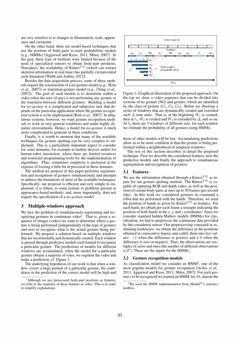
are very sensitive to to changes in illumination, scale, appear-ance and viewpoint.

On the other hand, there are model-based techniques thatuse the position of body-parts to train probabilistic models(e.g., HMMs) [Aggarwal and Ryoo, 2011; Mitra, 2007]. Inthe past, these type of methods were limited because of theneed of specialized sensors to obtain body-part positions.Nowadays, the availability of KinectTM (which can extractskeleton information in real time) has partially circumventedsuch limitation [Webb and Ashley, 2012].

Besides the data acquisition process, some of these meth-ods require the construction of a no-gesture model (e.g., [Kimet al., 2007]) or transition-gesture model (e.g., [Yang et al.,2007]). The goal of such models is to determine within avideo when the user (if any) is not performing any gesture orthe transition between different gestures. Building a modelfor no-gesture is a complicated and subjective task that de-pends on the particular application where the gesture recogni-tion system is to be implemented [Kim et al., 2007]. In ubiq-uitous systems, however, we want gesture recognition meth-ods to work in very general conditions and under highly dy-namic environments. Hence, a model for no-gesture is muchmore complicated to generate in these conditions.

Finally, it is worth to mention that many of the availabletechniques for gesture spotting can be very complex to im-plement. This is a particularly important aspect to considerfor some domains, for example in mobile devices and/or forhuman-robot interaction; where there are limited resourcesand restricted programming tools for the implementation ofalgorithms. Thus, sometimes simplicity is preferred at theexpense of loosing a little bit in precision in these domains.

The method we propose in this paper performs segmenta-tion and recognition of gestures simultaneously and attemptsto address the limitations of most of the available techniques.Specifically, our proposal is efficient and very simple to im-plement; it is robust, to some extend, to problems present inappearance-based methods; and, more importantly, does notrequire the specification of a no-gesture model.

3 Multiple-windows approachWe face the problem of simultaneously segmenting and rec-ognizing gestures in continuous video1. That is, given a se-quence of images (video) we want to determine where a ges-ture is being performed (independently of the type of gesture)and next to recognize what is the actual gesture being per-formed. We propose a solution based on multiple windowsthat are incrementally and dynamically created. Each windowis passed through predictive models each trained to recognizea particular gesture. The predictions of models for differentwindows are accumulated, when the model for a particulargesture obtains a majority of votes, we segment the video andmake a prediction, cf. Figure 1.

The underlying hypothesis of our work is that when a win-dow covers a large portion of a particular gesture, the confi-dence in the prediction of the correct model will be high and

1Although we use (processed) body-part positions as features,we refer to the sequence of these features as video. This is in orderto simplify explanations.

Figure 1: Graphical illustration of the proposed approach. Onthe top we show a video sequence that can be divided intosections of no gesture (NG) and gesture, which are identifiedby the class of gesture (G1, G2, G3). Below we illustrate aseries of windows that are dynamically created and extendedeach ∆ time units. That is, at the beginning W1 is created,then at t1, W2 is created and W1 is extended by ∆, and so on.At t5 there are 5 windows of different size, for each windowwe estimate the probability of all gestures using HMMs.

those of other models will be low. Accumulating predictionsallow us to be more confident in that the gesture is being per-formed within a neighborhood of temporal windows.

The rest of this section describes in detail the proposedtechnique. First we describe the considered features, next thepredictive models and finally the approach to simultaneoussegmentation and recognition of gestures.

3.1 FeaturesWe use the information obtained through a KinectTM as in-puts for our gesture spotting method. The KinectTM is ca-pable of capturing RGB and depth video, as well as the posi-tions of certain body-parts at rates up to 30 frames-per-second(fps). In this work we considered gestures to command arobot that are performed with the hands. Therefore, we usedthe position of hands as given by KinectTM as features. Foreach hand, we obtain per each frame a sextuple indicating theposition of both hands in the x, y, and z coordinates. Since weconsider standard hidden Markov models (HMMs) for clas-sification, we had to preprocess the continuous data providedby the considered sensor. Our preprocessing consisted in es-timating tendencies: we obtain the difference in the positionsobtained in consecutive frames and codify them into two val-ues: +1 when the difference is positive and a 0 when thedifference is zero or negative. Thus, the observations are sex-tuples of zeros and ones (the number of different observationsis 26). These are the inputs for the HMMs.

3.2 Gesture recognition modelsAs classification model we consider an HMM2, one of themost popular models for gesture recognition [Aviles et al.,2011; Aggarwal and Ryoo, 2011; Mitra, 2007]. For each ges-ture i to be recognized we trained an HMM, letMi denote the

2We used the HMM implementation from MatlabR’s statisticstoolbox.

30

HMM for the ith gesture, where i = {1, . . .K} when con-sidering K different gestures. The models are trained withthe Baum-Welch algorithm using complete sequences depict-ing (only) the gestures of interest. Each HMM was trainedfor a maximum of 200 iterations and a tolerance of 0.00001(the training process stops when changes between probabili-ties of successive transition/emission matrices do not exceedthis value); the number of states in the HMM was fixed to 3,after some preliminary experimentation.

For making predictions we evaluate the different HMMsover the test sequence using the Forward algorithm, see [Ra-biner, 1990] for details. We use the probabilities returned byeach HMM as its confidence on the gesture class for a partic-ular window.

3.3 Simultaneous segmentation and recognitionThe multi-windows approach to gesture segmentation andrecognition is as follows, see Figure 1. For processing a con-tinuous video we trigger windows incrementally: at time t0a temporal window W0 of length ∆ is triggered and all ofthe (trained) HMMs are evaluated in this window. At timet1 we trigger another window W1 of length ∆ and increasewindow W0 by ∆ frames, the HMMs are evaluated in thesetwo windows too. This process is repeated until certain con-dition is met (see below) or until window W1 surpass a max-imum length, which corresponds to the maximum number ofallowed simultaneous window, q.

In this way, at a time tg we have g− windows of varyinglengths, and the outputs of the K−HMMs for each window(i.e., a total of g×K probabilities, where K is the number ofgestures or activities that the system can recognize). The out-puts of the HMMs are given in the form of probabilities. Toobtain a prediction for each window i we simply keep the la-bel/gesture corresponding to the model that obtains the high-est probability in window i, that is, argmaxkP (Mk,Wi).

In order to detect the presence of a gesture in the continu-ous video we estimate at each time tj the percentage of votesthat each of the K−gestures obtains, by considering the pre-dictions for the j−windows. If the number of votes exceedsa threshold, τ , we trigger a flag indicating that a gesture hasbeen recognized. When the flag is on, we keep increasingand generating windows and storing predictions until there isa decrement in the percentages of votes for the dominant ges-ture. That is, end of the gesture happens in the frame wherethere is a decrement in the number of votes. Alternatively, wealso experimented with varying the window in which we seg-ment the gesture: we segmented the gesture 10 frames beforeand 10 frames after we detect the decrement in the percent-age of votes, we report experimental results under the threesettings in Section 4. At this instant the votes for each typeof gesture are counted, and the gesture with the maximumnumber of votes is selected as the recognized gesture. Once agesture is recognized, the system is reset; that is, all ongoingwindows are discarded and a the process starts again with asingle window.

One should note that the less windows we consider for tak-ing a decision the higher the chances that we make a mistake.Therefore, we ban the proposed technique for making pre-dictions before having analyzed at least p−windows. Under

these settings, our proposal will try to segment and recognizegestures only when the number of windows/predictions is be-tween (p, q).

Figure 2 illustrates the process for simultaneous segmenta-tion and recognition for a particular test sequence containingone gesture. The first three plots show the probabilities re-turned by the HMMs for three gestures; we show the proba-bilities for windows starting at different frames of the contin-uous sequence. The fourth plot shows the percentage of votesfor a particular gesture at different segments of the video.For this particular example, the proposed approach is able tosegment correctly the gesture (the boundaries for the gesturepresent in the sequence are shown in gray). In the next sec-tion we report experimental results obtained with our methodfor simultaneous segmentation and recognition of gestures.

4 Experimental resultsWe performed experiments with the multi-windows approachby trying to recognize gestures to command a robot. Specif-ically, we consider three gestures: move-right (MR), atten-tion (ATTN), move-left (ML), these are illustrated in Figure 3.For evaluation we generated sequences of gestures of varyinglengths and applied our method. The number of training andtesting gestures are shown in Table 1. Training gestures weremanually segmented. Test sequences are not segmented; theycontain a single gesture, but the gesture is surrounded by largeportions of continuous video without a gesture, see Figure 2.

Figure 3: The three gestures considered for experimentation.From left to right: move-right, attention, move-left.

Three different subjects recorded the training videos. Thetest sequences were recorded by six subjects (three of whichwere different from those that recorded the training ones).The skeleton information was recorded with the NUI Capturesoftware3 at a rate of 30fps. The average duration of traininggestures was of 35.33 frames, whereas the average durationof test sequences was of 94 frames (maximum and minimumdurations were of 189 and 55 frames respectively).

All of the parameters of our model were fixed after pre-liminary experimentation. The better values we found forthem are as follows: ∆ = 10; p = 30; q = 60; τ = 100.After training the HMMs individually, we applied the multi-windows approach to each of the test sequences.

We evaluate the segmentation and recognition performanceas follows. We say the proposed method correctly segments

3http://nuicapture.com/

31

Figure 2: Multi-windows technique in action. The first three plots show probabilities obtained per each HMM for windowsstarting at different times. In the bottom-right plot we show the number of votes obtained by the dominant HMM, note that thenumber of votes start to diminish, this is taken as an indication of the end of the gesture (best viewed in color).

Table 1: Characteristics of the data set considered for exper-imentation. We show the number of training videos per ges-ture, and, in row two, the number of gestures present in thetest sequences.

Feature MR ATTN MLTraining vids. 30 30 30Testing vids. 18 18 21

a video when the segmentation prediction is at a distance ofδ−frames (or less) from the final frame for the gesture; wereport results for δ = 5, 10, 15, 20. On the other hand, we saythe proposed method correctly recognizes a gesture, when thegesture predicted by our method (previously segmented) wasthe correct one.

Table 2 shows the segmentation and recognition perfor-mance obtained by the multi-windows approach. We reportresults when segmenting the gesture before, in and after thedecrement in percentage of votes is detected, see Section 3.

From Table 2 it can be observed that segmentation perfor-mance is low under a hard criteria (i.e., δ = 5 frames of dis-tance), the highest performance in this setting was of 29.82%.However, the recognition performance is quite high for thesame configuration, achieving recognition rates of 82.35%.Thus, the method offers a good tradeoff4 between segmenta-

4Despite the fact that segmentation performance may seem low,one should note that for the considered application it is not too badfor an user to repeat a gesture 3 times in order that a robot correctly

Table 2: Segmentation (Seg.) and recognition (Rec.) perfor-mance of the multi-windows technique. .

Before In Afterδ Seg. Rec. Seg. Rec. Seg. Rec.5 29.82% 82.35% 26.32% 60.00% 26.32% 80.00%10 54.39% 67.74% 63.16% 66.67% 50.88% 68.97%15 59.65% 64.71% 70.18% 67.50% 56.14% 68.75%20 78.95% 62.22% 80.70% 63.04% 73.68% 66.67%

tion and recognition performance.In order to determine how good/bad our recognition results

were, we performed an experiment in which we classified allof the gestures in test sequences after we manually segmentedthem (top-line). The average recognition performance for thatexperiment was of 85.96%. This performance represents thebest recognition performance we could obtain with the fea-tures and trained models. By looking at our best recognitionresult (columns Before, row 1), we can see that the recogni-tion performance of the multi-windows approach is very closeto that we would obtain when classifying segmented gestures.

As expected, segmentation performance improves whenwe relax the distance to the boundaries of the gesture (i.e.,for increasing δ). When the allowed distance is of δ = 20

identifies the command we want to transmit. Instead, accurate recog-nition systems are required so that the robot clearly understand theordered command, even when the user has to repeat the gesture acouple of times.

32

frames, we were able to segment up to 80% of the gestures.Recognition rates decreased accordingly. When we comparethe segmentation performance obtained when segmenting thegesture before, in or after the decrement of votes, we foundthat the performance was very similar. Although, segment-ing the gesture 10 frames before we detected the decrementseems to be a better option. This makes sense, as we wouldexpect to see a decrement of votes when the gesture alreadyhas finished.

Regarding efficiency, in preliminarily experiments we havefound the proposed method can run in near real-time. In astate-of-the art workstation, it can process data at a rate of30fps, which is enough for many human-computer interactiontasks. Nevertheless, we still have to perform a comprehensiveevaluation of our proposal in terms of efficiency and takinginto account that in some scenarios a high-performance com-puters are not available.

From the experimental study presented in this section wecan conclude that the proposed method is a promising solu-tion to the problem of simultaneous gesture segmentation andrecognition. The simplicity of implementation and the effi-ciency of our approach are beneficial for the development ofubiquious and human-centric systems.

5 Conclusions and future work directionsWe proposed a new method for simultaneous segmentationand recognition of gestures in continuous video. The pro-posed approach combines the outputs of classification mod-els evaluated in multiple temporal windows. These windowsare dynamically and incrementally created as the video usscanned. We report preliminary results obtained with the pro-posed technique for segmenting and recognizing gestures tocommand a robot. Experimental results reveal that the recog-nition performance of our method is very close to that ob-tained when using manually segmented gestures. Segmenta-tion performance of out proposal is still low, yet current per-formance is acceptable for the considered application. Thefollowing conclusions can be drawn so far:

• The proposed method is capable of segmenting gestures(with an error of 5 frames) at low-mild recognition rates.Nevertheless, these rates are accurate-enough for someapplications. Recall we are analyzing a continuous se-quence of video and that we do not require of a modelfor no-gesture, as required in related models.

• Recognition rates achieved by the method are acceptablefor a number of applications and domains. In fact, recog-nition results were very close to what we would obtainwhen classifying manually-segmented gestures.

• The proposed method is very easy to implement and canwork in near real-time, hence its applicability in ubiq-uitous data mining and human-centric applications arequite possible.

The proposed method can be improved in several ways, butit remains to be compared to alternative techniques. In thisaspect we have already implemented the method from [Kimet al., 2007], but results are too bad in comparison with our

proposal. We are looking for alternative methods to compareour proposal.

Current and future work includes extending the numberof gestures considered in this study and implementing themethod in the robot of our laboratory5. Additionally, weare working in different ways to improve the segmentationperformance of our method, including using different votingschemes to combine the outputs of the different windows.

References[Aggarwal and Ryoo, 2011] J. K. Aggarwal and M. S. Ryoo.

Human activity analysis: a review. ACM Computing Sur-veys, 43:16(3), 2011.

[Aviles et al., 2011] H.H. Aviles, L.E. Sucar, C.E. Mendoza,and L.A. Pineda. A comparison of dynamic naive bayesianclassifiers and hidden. Journal of Applied Research andTechnology, 9(1):81–102, 2011.

[Derpanis et al., 2010] K. G. Derpanis, M. Sizintsev, K. Can-nons, and R. P. Wildes. Efficient action spotting based ona spacetime oriented structure representation. In Proc. ofCVPR, pages 1990–1997. IEEE, 2010.

[Eunju, 2010] K. Eunju. Human activity recognition and pat-tern discovery. Pervasive Computing, 9(1):48–53, 2010.

[Huynh et al., 2008] T. Huynh, M. Fritz, and B. Schiele. Dis-covery of activity patterns using topic models. In Proc. ofUbiComp’08, pages 10–19. ACM Press, 2008.

[Kim et al., 2007] D. Kim, J. Song, and D. Kim. Simulta-neous gesture segmentation and recognition based on for-ward spotting accumulative hmms. Pattern recognition,40(11):3012–3026, 2007.

[Malgireddy et al., 2012] M.R. Malgireddy, I. Inwogu, andV. Govindaraju. A temporal bayesian model for classify-ing, detecting and localizing activities in video sequences.In Proc. of CVPRW, pages 43–48, 2012.

[Mitra, 2007] S. Mitra. Gesture recognition: a survey. IEEETransactions on Systems, Man, and Cybernetics, Part C,37(3):311–324, 2007.

[Rabiner, 1990] L. E. Rabiner. Readings in speech recogni-tion, chapter A tutorial on hidden Markov models and se-lected applications in speech recognition, pages 267–296.Morgan Kaufmann, 1990.

[Webb and Ashley, 2012] J. Webb and J. Ashley. Begin-ning Kinect Programming with the Microsoft Kinect SDK.Apres, 2012.

[Yang et al., 2007] H.D. Yang, A. Y. Park, and S. W. Lee.Gesture spotting and recognition for humanrobot inter-action. IEEE Transactions on robotics, 23(2):256–270,2007.

[Yuan et al., 2009] J. Yuan, Z. Liu, and Y. Wu. Discrimi-native subvolume search for efficient action detection. InProc. of CVPR. IEEE, 2009.

5http://ccc.inaoep.mx/ markovito/

33

Cicerone: Design of a Real-Time Area Knowledge-Enhanced Venue Recommender

Daniel Villatoro, Jordi Aranda, Marc Planagumà, Rafael Gimenez and Marc Torrent-MorenoBarcelona Digital Technology Centre, Barcelona, Spain

{dvillatoro,jaranda,mplanaguma,rgimenez,mtorrent}@bdigital.org

Abstract

Smart-devices with information sharing capabili-ties anytime and anywhere have opened a widerange of ubiquitous applications. Within urban en-vironments citizens have a plethora of locations tochoose from, and in the advent of the smart-citiesparadigm, this is the scope of location-based rec-ommender systems to provide citizens with the ad-equate suggestions. In this work we present the de-sign of an in-situ location-based recommender sys-tem, where the venue recommendations are builtupon the users’ location at request-time, but alsoincorporating the social dimension and the exper-tise of the neighboring users knowledge used tobuild the recommendations. Moreover, we proposea specific easy-to-deploy architecture, that bases itsfunctioning in the participatory social media plat-forms such as Twitter or Foursquare. Our systemconstructs its knowledge base from the accesibledata in Foursquare, and similarly obtains ratingsfrom geopositioned tweets.

1 IntroductionUrban environments host a plethora of interesting locationssuch as restaurants, shops, museums, theaters and a widerange of other venues that neither can be known by all usersnor they might be interested in visiting all. However, eachcitizen can potentially become an expert of the neighborhoodhe visits more often or lives, as he will know, and maybe havevisited, more venues in such area. Therefore, it is straighfor-ward to see how for an specific citizen might not be a problemto find an adequate venue for his taste on his neighborhood ofexpertise, but it potentially becomes cumbersome to do thesame task when in a different less-known neighborhood. Itbecomes then a problem for citizens to find locations theymight enjoy when away of their area of expertise. The prob-lem of finding adequate items for specific users is that clasi-cally solved by recommender systems.In our case, we focus on location-based recommender sys-tems [Zheng et al., 2009; Park et al., 2007], where users arerecommended locations to visit expecting to maximize users’satisfaction. These type of recommenders complement the

previously analyzed ones as they also have to take into ac-count the context, distance from the user to the recommendedvenue, and maybe several other factors.With the penetration of smart-devices, users have the pos-sibility to access information anytime anywhere, and thesystem we present in this work profits from those ubiqui-tious computing capabilities; our on-site location-based rec-ommender system allows users to obtain the most adequatevenue with respect to their current position. Our approachprofits from a different dimension of the users’ parametersspace, namely their social relationships and their relative geo-graphical knowledge with respect to the location of the items.This model provides an alternative solution to the problemof providing personalized recommendations in a geospatialdomain: user expertise in this type of domain conveys animplicit continuum knowledge of the surrounding geospatialarea and the locations within that area. Our solution intelli-gently combines this user geospatial knowledge to the clas-sical social distances amongst users used in state-of-the-artrecommenders.Our system personalizes recommendations of locations notonly considering the past history of a specific user, but also(1) the current location of the user, (2) the social distance withother similar users and (3) their expertise in the area wherethe recommendation is going to be provided. This aggrega-tion function basically expresses a tendency of a user to visita certain location given its distance to the location, and thepast history of the user and its friends and their knowledge ofthe area.To the best of our knowledge, there are no existing recom-mender systems that profit from the inherent characteristics ofthe geographical location, such as continuity in space, user’sarea expertise or word-of-mouth location suggestions, to gen-erate recommendations to users.

2 State of the ArtAs we have discussed previously, the problem of finding ad-equate venues for citizens to visit is a problem already tack-led by the recommender community, under the location-basedrecommender systems [Zheng et al., 2009; Park et al., 2007].Despite the impressive amount of literature in such area, thisis still an open problem, even for those with access to com-plete datasets and user profiles [Sklar et al., 2012], as newmethods and algorithms are being proposed to boost their ef-

34

ficiency.In this work however, we propose the integration of social in-formation into the calculation of the recommendations. Someautors have investigated the potential of the explicit inclusionof information of user’s relationships from social networks togenerate the neighborhood used in classical collaborative fil-tering (CF) algorithms (social filtering), improving the resutlsobtained by the classic CF in the analyzed scenarios [Grohand Ehmig, 2007].Others [Bonhard and Sasse, 2006] have analyzed how therelationship between advice-seeker and recommender is ex-tremely important in the user-centered recommendations,concluding that familiarity and similarity amongst the dif-ferent roles in the recommendation process aid judgementand decision making. As well as in our approach, some re-searchers have considered the important role of experts [Am-atriain et al., 2009; Bao et al., 2012], however in our case,these experts are calculated automatically for each specificarea of the city and weighted with respect to the social dis-tance amongst the advice-seeker and recommender.A similar recommendation approach is presented [Ye et al.,2010], where authors also propose the usage of Foursquareinformation to provide venue recommendations to users;more importantly the social perspective is integrated into theirrecommendations, developing a Friend-Based CollaborativeFiltering (where the neighbours for CF are selected from thesocial network of users), and an extension of this methodGeo-measured Friend-Based Collaborative Filtering (whereonly closely located friends are selected as neighbours forCF).Our method then proposes a combination of the Geo-measured Friend-Based Collaborative Filtering [Ye et al.,2010] and experts [Amatriain et al., 2009; Bao et al., 2012],in our specific case, neighborhood or area experts.

3 Cicerone Recommender SystemIn this section we provide the theoretical framework of theCicerone location-based recommender system. Firstly we de-scribe the basic terminology used later in the recommenda-tion algorithm. As we have sketched previously, our systembases its functioning in three information elements: the users’social network, the users’ area knowledge and the current lo-cation of the requesting user.

3.1 Basic TerminologyAs used herein, the term “location data item” stands for anylocation item or representation of a location. A “locationitem” is intended to encompass any type of location whichcan be represented in a map using a latitude, a longitude, andpossibly a category.

The location recommender may be capable of selecting rel-evant locations for a given target user. To do so, users shouldbe comparable entities and locations as well. It should beunderstood that the implementations described herein are notitem-specific and may operate with any other type of item vis-ited/shared by a community of users. For the specific case ofbars or restaurants items, users may interact with the items byvisiting them. The Recommendations Set is the locations set

formed by the items the user is being recommended. A UserA’s Recommendations set will be denoted herein as RA.

An essential concept is the one of “Check-in” (CItU,L)which represents the attendance1 of a user U to a certain lo-cation L in the last t days, and therefore. Our system willgenerate Location recommendations to the users by consid-ering not only its geographical position, but also its socialrelationship with other users and their degree of knowledgeof the visited locations.

In order to obtain more adequate recommendations in thistype of environments, we envision the necessity of certainestimators. Firstly, we need to quantify how well a certainuser knows a specific area (by considering the attendance fre-quency to locations in such area with respect to the rest ofthe city). Moreover, it becomes necessary to understand thesocial distance between the target user and the other users,whose opinions are being used to create the recommendationsfor the target user.

These measures are clearly described and specified next:The Area Knowledge (AKt

U,L) of a user U with respect to alocation L is calculated:

AKtU,L =

∑l′∈PostalCodeL

CItU,l′

∑∀a∈Locations

CItU,a

(1)

and represents how familiar a user is within an specific areaof the city (represented by its postal code).The Location Frequency (LF t

U,L) of a user U in a certainlocation L is calculated:

LF tU,L =

CItU,L∑∀a∈Locations

CItU,a

(2)

and normalizes the number of visits of the user U to the loca-tion L.The Social Importance (SItU,U ′ ) of a user U ′ for a user U iscalculated:

SItU,U ′ =(DegreeU ′)

1d(U,U′)

(nodes− 1)(3)

where DegreeU represents the number of connectionsthat U has in its social network, nodes represents the totalnumber of nodes in the social network (and used to normalizethe SI), and d(U,U ′) represents the geodesic distance, i.e.minimum number of hops necessary to reach U ′ from Uusing the shortest path in their social network2.

The Location Value (LV tL,U ) of a location L for a user U

at time t is calculated:

LV tL,U =

∑usersinL

(LF tU,L ×AKt

U,L × SItU,U ′)

|users| (4)

1The attendance of a user to a certain location can be captured inseveral ways, for example, a Foursquare Check-in, a geopositionedtweet, or a CDR trace of a phone call.

2d(U,U ′) < 0 means that there is no possible path that connectsU and U ′

35

Figure 1: Twitter-sensed Barcelona Social Network

where |users| represents the number of users that have“checked-in” to that Location.

The resulting value basically aggregates the informationof surrounding detected locations considering the social dis-tance of our specific user to the users that visited that location(social information), and their familiarity in the area of thelocation (geographical information).

3.2 Cicerone Recommendation AlgorithmThe general algorithm for the functioning is the following:

1. Once the position of a user A is detected, the systemautomatically captures its Latitude and Longitude andlaunches the process that builds the personalized recom-mendation set for that position and user at that certainmoment.

2. The system retrieves all the locations in 100m radius ofthe current position.

3. The recommendation set for user A, Ra, is a set con-structed with all the locations in 100m radius of the usercurrent position.

4. The system calculates the location value of each of thelocations in that set.

5. The system orders the retrieved locations according tothe calculated Location Values and constructs the Rec-ommendation Set with the 3 with a highest value.

4 Functional implementation of CiceroneAs explained previously, the theoretical framework to buildthe recommendation needs from a number of data sources,namely, users locations, venues and the social relationshipsamongst users. As this recommendation process is envisionedto be executed when users are in-situ, the main functional re-quirement for our system is to work from a mobile device.Working prototypes have decided to opt for the developmentof a dedicated app (such as Yelp, TimeOut or TripAdvisor),that users have to download within their devices. The appprovides several advantages as the explicit user profiling aswell as the definition of the necessary information to obtainthe recommendation. However, for us it implies the big prob-lem of reaching a critical mass of users that would made theknowledge base and the recommendation more accurate. Toavoid this limitation we have opted to develop our system as

a service embedded within already massive social networks.Twitter seems to be the ideal candidate for us for the follow-ing reasons:

• Twitter shows a widespread uniform penetration almostworldwide, with an continously increasing numebr ofusers (288 million monthly active users in July 2012,showing an increase of 40% since July 2009 [Global-WebIndex, 2013]).

• It allows users to associate their location when posting amessage, and associate the specific coordinates as meta-information.

• It provides developers with an accesible API to obtain innear real-time the publicly published tweets.

• Twitter captures a social network of followers and fol-lowings, publicly available for each user.

As we have initially decided to deploy our application in thecity of Barcelona, Twitter confirms to be an ideal candidate.The number of captured geopositioned tweets daily withinBarcelona is 6200 (from data coming from 2012), and thesocial network inferred from the users posting them can beseen in Figure 1 (with an average degree of 2.93).

Similarly, and to populate our items database, we opt touse the crowdsourced database of Foursquare. Foursquare isa location-based social media platform to communicate thevenues a user is in. This platform allows users to input intotheir databases new locations, by introducing not only thevenue’s name and specific location (with the GPS positionand postal address) but also a semantic category. Foursquaredescribes the places according to a rather complete taxonomy,where about 400 kinds of places are identified and grouped in9 wide categories3. Foursquare provides an accesible API al-lowing us to take snapshots of the existing locations in a cer-tain city. Within the city of Barcelona, from a snapshot takenApril 2013, we have detected over 66.000 foursquare loca-tions, uniformly distributed amongst the different districts.

Moreover, within the OpenData movement, the city ofBarcelona provides a machine-readable administrative divi-sion necessary for our theoretical calculations (namely theDistrict divisions).

5 System ArchitectureIn this section we will describe the system architecture(sketched in Figure 2) needed to implement a functional in-statiation of the theoretical framework previously described.Firstly we will describe the social network monitoring usedas data input for our platform, and also as user interface inter-action with the recommendation engine. After that, we willsketch the persistence infrastructure used to save the informa-tion related to venues and users, and finally we will describethe information update process and the component needed todevelop the recommendation platform.

3The detailed categorization of Foursquare categories and parentcategories can be found at http://aboutfoursquare.com/foursquare-categories/ (Last access April 2nd 2013).

36

Figure 2: Cicerone Architecture

Figure 3: Cicerone Workflow

5.1 Social Networks Monitoring: Sensing the CityThe usage of social media platforms in our system aretwofold: (1) information acquisition to feed the knowledgebase of our platform, and (2) a channel for users’ interactionwith our technology.

The participatory information provided by users inFoursquare will be used to populate our items database; sim-ilarly, we will use geopositioned tweets to calculate users’Area Knowledge. Therefore, the social network monitor isthe first layer of our architecture and it is composed by twocrawlers: a Foursquare crawler and a Twitter crawler. TheFoursquare crawler is in charge to scan the target city for newvenues. Once a new venue is identified, it is stored in theitems database with its associated metainformation such asits specific coordinates, the address or the category. The Twit-ter crawler is in charge to capture all the tweets generated inthe target city. Its scope is threefold: (1) build and updatethe users’ social network, (2) update the user area knowledgeusing its geopositioned tweets, and (3) permits users’ com-munication with the system.

Moreover, and given its popularity, we use Twitter as thecommunication channel of our recommender system througha bot account managed by our intelligent agent.

5.2 Persistence Infrastructure: Urban data ModelAny recommender system bases its functioning in three mainelements: users, items and ratings. These three elements haveto be stored according to the inherent properties of the sys-tem, which in this case, imply real-time information access

and update. Fed by the crawlers, the data required for our rec-ommendation solution arrives to the persistence manager andeach of these elements are stored in a persistence infrastruc-ture in the following way: Users: One of the main functionalrequirements of the recommendation algorithm is the accessto the social network of users. In order to effectively storethis information, we opt for using a graph-oriented database,namely Neo4j4. These type of databases allow us to per-sist users’ social network in the form of a directed weightedgraph. In this database, we persist users as nodes and thenestablish edges amongst nodes if there exist a social relationamongst them. Consequently, an edge between two nodes iscreated if there exists a social relation amongst them, accord-ing to users’ Twitter profiles; specifically, an edge is createdamongst from user A towards user B if userA follows user Bin Twitter. At this edge level, the edge’s weight will be de-fined depending on the users interactions: different types ofTwitter interactions (such as mentions, retweets or favourited)will affect the weight differently.5 Another important infor-mation about users is saved, namely his “Check-ins” (as de-scribed in Sec. ). These “check-ins” (the specific coordinatesof each user geopositioned tweet) is stored into a MongoDB6,as we can profit from the implemented geo-spatial index.Items: The items in our system are the locations within thetarget city. The locations database needs to provide efficientinformation access, as the recommender algorithm needs ahigh average number of accesses to it to build the recom-mendations. Moreover, an imporant item’s characteristic isits location within space, that is proffited from when usinggeo-spatial indexing. Given these two characteristics (rapidinformation access and geo-spatial indexing), as well as thepotential for distributed computing, we opt to implement thisdatabase using MongoDB.Ratings: The notion of rating is clasically treated as an ex-plicit evaluation of users about an item. However, in thiswork, we take an alternative approach for ratings: we con-sider as a constant rating value the users presence in a loca-tion, sensed through the geopositioned tweets posted from orclose to the venue location. This value is not obtained di-rectly, the Ratings will be part of knowledge obtained by therecomendation engine and their information update processcapturing user’s visits to specific locations but this will be ex-plained on the Section 5.3.

5.3 Recomendation Engine: Information UpdateProcess

The last component in our proposed architecture is the re-comendation engine containing the implementation of thetheoretical algorithms previously explained in the Section 3.Once we have our social networks monitor as an urban datasensor, and the ability to persist all the raw data requiredby the system, this component will be the responsible of theknowledge extraction process and the bussines logic triggered

4http://www.neo4j.org5Specific values and functions for edge weight determination

will be developed at later versions of our software using empiricalinformation.

6http://www.mongodb.org

37

to generate a recommendation.Because of the real-time aspect of our system, our recom-

mendation platform (whose workflow is detailed in Figure 3)needs to continously update some information elements suchas users’ Area Knowledge and Location Frequency, the cre-ation or update of social relationships amongst users or theappearance of new locations. Specifically, we envision theusers’ communication with our system through a Twitter per-sonality that encapsules our recommendation platform; ev-erytime a user mentions our system’s username, the plat-form will capture this tweet (through the Mention’s Servicesketched in Figure 2) and identify it as an explicit requestfor a recommendation that will trigger the whole intelligentprocess. Eventhough our technological platform allows us togenerate recommendations everytime a user’s location is cap-tured (with every geopositioned tweet), we rather restrict itsfunctioning with a mention system reducing the overall intru-siveness.

After the recommendation is generated, it is returned tothe user also through Twitter with a message posted by ourintelligent agent.

6 Conclusion and Future WorkThe designed recommender system plans to profit from theinformation proactively shared by users in the analyzed par-ticipatory platforms. However, as recently argued in [Jeske,2013], these type of crowdsourced systems is sensible to ma-licious attacks: in our case, and given the lack of restrictionsto post geo-positioned content from Twitter, someone couldeasily envision the method to create a fake user to become theone with higher area knowledge in every area of the city, andthen influence directly the resulting recommendations to hisown will.

Despite this potential problem associated to the publishingpolicy of Twitter and Foursquare, and as we have analyzed inSec. 2, many others have used information from these sourcesto generate location-based recommendations. However, andto the best of our knowledge, the presented algorithm is thefirst to include explicitly the user’s expertise about one of thefundamental properties of the items: the area where it is lo-cated. By combining this information, with some social infor-mation, we hypothesize that our system will be able to out-perform other location-based recommender systems.

Our main long term research task to be performed is thedevelopment of a user profiling in term of the type of venuesthe user attends to, with the overall objective of combiningthe area expertise and with specific user profiles.

AcknowledgmentsThis work has been completed with the support of ACC1Ó,the Catalan Agency to promote applied research and innova-tion.

References[Amatriain et al., 2009] Xavier Amatriain, Neal Lathia,

Josep M. Pujol, Haewoon Kwak, and Nuria Oliver. Thewisdom of the few: a collaborative filtering approach

based on expert opinions from the web. In Proceedingsof the 32nd international ACM SIGIR conference on Re-search and development in information retrieval, SIGIR’09, pages 532–539, New York, NY, USA, 2009. ACM.

[Bao et al., 2012] Jie Bao, Yu Zheng, and Mohamed F. Mok-bel. Location-based and preference-aware recommenda-tion using sparse geo-social networking data. In Proceed-ings of the 20th International Conference on Advancesin Geographic Information Systems, SIGSPATIAL ’12,pages 199–208, New York, NY, USA, 2012. ACM.

[Bonhard and Sasse, 2006] P. Bonhard and M. A. Sasse.’knowing me, knowing you’ – using profiles and socialnetworking to improve recommender systems. BT Tech-nology Journal, 24(3):84–98, July 2006.

[GlobalWebIndex, 2013] GlobalWebIndex. Twitter now thefastest growing social platform in the world. Web Report,Jan 2013.

[Groh and Ehmig, 2007] Georg Groh and Christian Ehmig.Recommendations in taste related domains: collaborativefiltering vs. social filtering. In Proceedings of the 2007international ACM conference on Supporting group work,GROUP ’07, pages 127–136, New York, NY, USA, 2007.ACM.

[Jeske, 2013] Tobias Jeske. Floating car data from smart-phones: What google and waze know about you and howhackers can control traffic. https://media.blackhat.com/eu-13/briefings/Jeske/bh-eu-13-floating-car-data-jeske-wp.pdf (Last access April 1st 2013)., 2013.

[Park et al., 2007] Moon-Hee Park, Jin-Hyuk Hong, andSung-Bae Cho. Location-based recommendation systemusing bayesian users preference model in mobile devices.In Ubiquitous Intelligence and Computing, pages 1130–1139. Springer, 2007.

[Sklar et al., 2012] Max Sklar, Blake Shaw, and AndrewHogue. Recommending interesting events in real-timewith foursquare check-ins. In Proceedings of the sixthACM conference on Recommender systems, RecSys ’12,pages 311–312, New York, NY, USA, 2012. ACM.

[Ye et al., 2010] Mao Ye, Peifeng Yin, and Wang-Chien Lee.Location recommendation for location-based social net-works. In Proceedings of the 18th SIGSPATIAL Interna-tional Conference on Advances in Geographic InformationSystems, GIS ’10, pages 458–461, New York, NY, USA,2010. ACM.

[Zheng et al., 2009] Yu Zheng, Yukun Chen, Xing Xie, andWei-Ying Ma. Geolife2. 0: a location-based social net-working service. In Mobile Data Management: Systems,Services and Middleware, 2009. MDM’09. Tenth Interna-tional Conference on, pages 357–358. IEEE, 2009.

38

Road-quality classification and bump detection with bicycle-mounted smartphones

Marius Hoffmann, Michael Mock, Michael MayFraunhofer IAIS

Schloss Birlinghoven, 53754 St Augustin, Germanyfirst.lastname@iais.fraunhofer.de

AbstractThe paper proposes a embedded surface road clas-sifier for smartphones used to track and classifyroutes on bikes. The main idea is to provide, alongwith the route tracking, information about surfacequality of the cycling route (is the surface smooth,rough or bumpy?). The main problem is the quan-tity of accelerometer data that would have to be up-loaded along with GPS track, if the analysis wasdone off-line. Instead, we propose to classify roadsurfaces online with an embedded classifier, thathas been trained off-line. More specifically, we relyon the accelerometer of a bicycle-mounted smart-phone for online classification. We carry out exper-iments to collect cycling tracks consisting of GPSand accelerometer data, label the data and learn amodel for classification, which again is deployedon the smartphone. We report on our experienceswith classification accuracy on and runtime perfor-mance of the classifier on the smartphone.

1 IntroductionThe main motivation of this work is to provide a communitybased cycling route road quality classification service. Thereare many community based services providing cycling routestogether with altitude profiles, but none of them is providinginformation about the road quality of the route, i.e. whetherthe road is smooth, rough, or bumpy. Many bicycling com-munity web-portals like [http://www.bikemap.net] offer facil-ities for uploading and downloading GPS tracks for cyclingroutes. To our knowledge, none of them provides informationabout road surface quality of the cycling route. Route qualityinformation could be gathered together with GPS track usingthe accelerometer data coming from bicycle mounted smart-phone. Obviously, including all accelerometer raw data in thedata upload would increase data traffic significantly and maynot be tolerable for the user, especially when gathering longtracks. The solution is to implement a road surface classifi-cation algorithm on the smartphone and to upload the clas-sification results together with the GPS track. Similar ap-proaches already have been successfully applied for other ve-hicles than bicycles. Pothole detection using GPS data andaccelerometer data with dedicated hardware devices mounted

in Taxi cabs has already been successfully explored in [Eriks-son et al., 2008], [Strazdins12 et al., 2011] and [Mednis etal., 2012] investigate road condition monitoring for vehicularsensor networks based on time series analysis. We investi-gate experimentally, whether we can achieve a road surfaceclassification using smartphones mounted on bicycles. In or-der to cope with the restricted computational power of thesedevices, we apply a machine learning approach: we learn aclassifier off-line on a standard PC and apply the classifieronline on the smartphone.

We collected GPS tracks and acceleration data (based onthe mobile phone’s accelerometer sensor) and applied twodifferent approaches for classification of road surface qual-ity, both based on standard machine learning classifiers: ina direct segmentation classification approach, we used man-ual labeling of road segments of fixed length (smooth, rough,bumpy) to train a classifier, based of various parameter set-tings for feature extraction. The best result that we obtainedin a cross-validation was a 20% increase of accuracy against astandard Kappa-Statistics. In a second approach, we traineda classifier for detecting bumps. Here we achieved an ac-curacy of 97%. Using this bump detector, we performed athreshold-based road segment classification, which deliveredmuch more comprehensible results. A closer look at inputdata, manual labeling, classification results, and comparisonwith the real-world, revealed that the manual labeling was er-ror prone . We conclude that the simple bump-detector basedclassification approach can be used for road surface qualityclassification and even does not require further manual label-ing of road segments.

2 Classification approach and ResultsMost of today’s smartphones are equipped with GPS and ac-celeromater sensors. In order to ensure that our algorithmperforms not only on today’s top range models, we carriedout the experiments with a 2-years old Nokia 5800, one ofthe first mass models providing accelerometer data. Figure1 illustrates a track of accelerometer data collected with asmartphone.

Figure 1 shows the length of the accelerometer vector plot-ted over a track. We see that the data provides a more orless continuos signal (at 37 Hz in our case) over the completetrack. As we want to explore a machine learning classifica-tion approach for road surface classification, we first have to

39

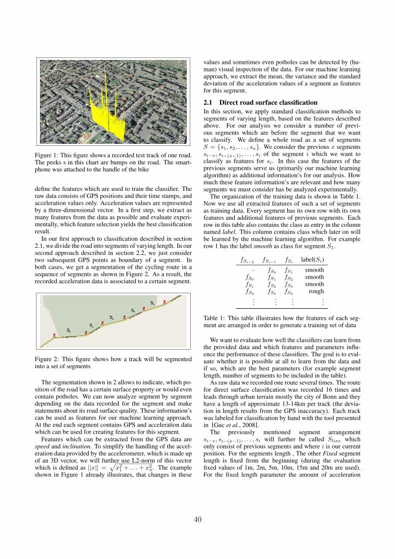
Figure 1: This figure shows a recorded test track of one road.The peeks s in this chart are bumps on the road. The smart-phone was attached to the handle of the bike

define the features which are used to train the classifier. Theraw data consists of GPS positions and their time stamps, andacceleration values only. Acceleration values are representedby a three-dimensional vector. In a first step, we extract asmany features from the data as possible and evaluate experi-mentally, which feature selection yields the best classificationresult.

In our first approach to classification described in section2.1, we divide the road into segments of varying length. In oursecond approach described in section 2.2, we just considertwo subsequent GPS points as boundary of a segment. Inboth cases, we get a segmentation of the cycling route in asequence of segments as shown in Figure 2. As a result, therecorded acceleration data is associated to a certain segment.

Figure 2: This figure shows how a track will be segmentedinto a set of segments

The segmentation shown in 2 allows to indicate, which po-sition of the road has a certain surface property or would evencontain potholes. We can now analyze segment by segmentdepending on the data recorded for the segment and makestatements about its road surface quality. These information’scan be used as features for our machine learning approach.At the end each segment contains GPS and acceleration datawhich can be used for creating features for this segment.

Features which can be extracted from the GPS data arespeed and inclination. To simplify the handling of the accel-eration data provided by the accelerometer, which is made upof an 3D vector, we will further use L2-norm of this vectorwhich is defined as ||x|| =

√x21 + . . .+ x2n. The example

shown in Figure 1 already illustrates, that changes in these

values and sometimes even potholes can be detected by (hu-man) visual inspection of the data. For our machine learningapproach, we extract the mean, the variance and the standarddeviation of the acceleration values of a segment as featuresfor this segment.

2.1 Direct road surface classificationIn this section, we apply standard classification methods tosegments of varying length, based on the features describedabove. For our analysis we consider a number of previ-ous segments which are before the segment that we wantto classify. We define a whole road as a set of segmentsS = {s1, s2, . . . , sn}. We consider the previous x segmentssi−x, si−(x−1), . . . , si of the segment i which we want toclassify as features for si. In this case the features of theprevious segments serve us (primarily our machine learningalgorithm) as additional information’s for our analysis. Howmuch these feature information’s are relevant and how manysegments we must consider has be analyzed experimentally.

The organization of the training data is shown in Table 1.Now we use all extracted features of such a set of segmentsas training data. Every segment has its own row with its ownfeatures and additional features of previous segments. Eachrow in this table also contains the class as entry in the columnnamed label. This column contains class which later on willbe learned by the machine learning algorithm. For examplerow 1 has the label smooth as class for segment S1.

fSi−2fSi−1

fSilabel(Si)

- fS0fS1

smoothfS0

fS1fS2

smoothfS1

fS2fS3

smoothfS2

fS3fS4

rough...

......

...

Table 1: This table illustrates how the features of each seg-ment are arranged in order to generate a training set of data

We want to evaluate how well the classifiers can learn fromthe provided data and which features and parameters influ-ence the performance of these classifiers. The goal is to eval-uate whether it is possible at all to learn from the data andif so, which are the best parameters (for example segmentlength, number of segments to be included in the table).

As raw data we recorded one route several times. The routefor direct surface classification was recorded 16 times andleads through urban terrain mostly the city of Bonn and theyhave a length of approximate 13-14km per track (the devia-tion in length results from the GPS inaccuracy). Each trackwas labeled for classification by hand with the tool presentedin [Guc et al., 2008].

The previously mentioned segment arrangementsi−x, si−(x−1), . . . , si will further be called Sline whichonly consist of previous segments and where i is our currentposition. For the segments length , The other Fixed segmentlength is fixed from the beginning (during the evaluationfixed values of 1m, 2m, 5m, 10m, 15m and 20m are used).For the fixed length parameter the amount of acceleration

40

values can vary, because the amount of values is speeddependant. For classification we will use two differentAlgorithms the K-Nearest-Neighbor and the Naıve BayesianClassifier. Five different features were extracted fromthe training data :speed, inclination, acceleration mean,acceleration variance, acceleration standard deviation.

The following table shows a compact overview of all pa-rameters which were evaluated.

Parameter type Parameter ValueML-algorithm K-NN, Naive Bayes

segments lengths variabe length: gpsfixed length: 1m, 2m, 5m, 10m, 15m, 20m

number of segments 3, 5, 7, 9, 11, 13extracted features inclination, speed, acceleration (mean, variance, std)

Table 2: This table gives an overview of all parameters whichwere changed during evaluation. The acceleration containsthree features, acceleration-mean, -variance and -standard de-viation)

To measure the performance of the classification algorithmon the evaluation data, a 10-folded cross-validation was in-cluded. A N -folded cross validation splits the test data intoN equally large sets and then uses N − 1 set for training toclassifier and 1 set for validating the learned concept this is re-peated N times where for every iteration a different set of theN sets is used for validation. At the end a confusion matrixis provided from the cross-validation module which consistsof the average performance values of the classification.

Additionally we performed a feature selection optimizationin order to find the best feature combination. This optimiza-tion allows to find a feature combination wich only containsfeatures which influence the learning algorithm positivly andresult in hoch accuracy. Features which confuse the learningscheme will not be selected anymore. We found thaht the pre-viously mentioned speed and inclination feature confuses thelearning scheme and results in performances which are worsethan the corresponding kappa statistics.

true smooth true bumpy true rough class precisionpred. smooth 5785 882 92 85,590%pred. bumpy 836 1052 62 53,949%pred. rough 151 110 492 65,339%

class recall 85,425% 51,468% 76,161% accuracy: 77,457%

Table 3

The classification performance for the Naive Bayes and theK-NN were almost similar, but the K-NN performed (on av-erage) slightly better than the Naive Bayes.

For K-NN algorithm, the performance increases with anincreasing number of the segments which are consideredfor classification. The Naive Bayes classifier, however, hasa more constant performance, independently of the num-ber of segments included in the table. The evaluation alsoshowed that the classification results which use longer seg-ments lengths (15m and 20m) perform much better than theones with short segment length’s (2m). When looking at the

influences of all features, we observed that the speed featuredoes not contribute to the classification. The inclination fea-ture, even worse, confuses the classifier.

The best results (table 3) are achieved with the features ac-celeration (mean, variance, standard deviation) and a segmentlength of 20m and 13 segments must be considered for classi-fication. The used segment setup is the Sline setup. The cor-responding kappa statistic achieves an accuracy of 56,357%which makes a difference of 21,101% between the classifierand its kappa statistic.

The overall results of the classification (at best 78%) arenot very satisfying for a classification model. We will see insection 2.2 that the bump detection just based on GPS-definedsegments performs much better.

2.2 Bump detection based classificationIn this approach, we first consider the detection of sin-gle bumps or potholes. The classifier in this first just dis-tinguishes the two classes: ”bump” and ”no bump”. Forthe bump classification a different route was selected andrecorded 15 times. Each of them has a length between 110mand 130m per track (here the deviation in length also resultsfrom the GPS inaccuracy). Again each track was labeled forclassification by hand via the already mentioned annotatortool.

The performance of the bump classification works outmuch better compared to the highest accuracy of the sur-face classification. Again, the feature ”speed” turned out tobe irrelevant and the feature ”inclination” was confusing theclassifier. It was also observed that (for surface- not bump-classification), the more segments are considered the morethe accuracy declines. The reason for this is that the longerthe considered area the more unimportant information is con-tained in the data which should be classified. In compari-son to the surface classification, the bump classification needsshorter segment length’s (1m to 5m) to reach high classifica-tion accuracy. The longer the segment lengths, the worse theclassification performance gets. The long segment also con-fuse the classification algorithm, this was verified by com-paring the results of the classification with the correspondingkappa statistic. The best result were achieved with the seg-ment length GPS parameter. This is quite expected, because”bumps” are short term events and GPS-based segmentation(i.e. every two succeeding GPS points define a segment) isthe smallest achievable spatial granularity.

true no bump true bump class precisionpred. no bump 404 6 98,537%

pred. bump 2 29 93,548%

class recall 99,507% 82,857% accuracy: 98,186%

Table 4

As we can see it is indeed possible to do pothole andbumpy detection with a very high accuracy, just using theNaive Bayes Classifier on a single segment. This led us toextend this simple approach to be applicable in road surface

41

classification, with the three classes ”smooth”, ”rough”, and”bumpy”, as described in the following.

Extended bump classification The bump detection can bealtered slightly to derive another concept for surface classi-fication. The main idea is to count the number of bumpysegments in a certain road section. Depending on that num-ber, one of the classes ”smooth”, ”rough”, and ”bumpy” isassigned as follows:• For 0 ≤ |bumps| ≤ N

3 , the class smooth is assigned.

• For N3 < |bumps| ≤ 2N

3 , the class rough is assigned

• For 2N3 < |bumps| ≤ N , the class bumpy is assigned

Not surprisingly, the best results were achieved for N=3,i.e. just considering the GPS-Segments Si−1, Siand Si+1 forthe classification of GPS-segment Si. In other words, a GPSsegment is considered as, for example, smooth, if at most oneof its preceding, the GPS-segment itself, and the succeedingGPS-segment have a bump. The results are shown in Table 5.

true smooth true bumpy true rough class precisionpred. smooth 27865 1113 2129 89,578%pred. bumpy 2249 1823 3315 24,678%pred. rough 1488 537 2893 58,825%

class recall 88,175% 52,491% 34,701% accuracy: 75,051%

Table 5: Confusion matrix of a the best performing classifi-cation which considered 3 segments during its classification

The classifier with the best accuracy for surface classifica-tion achieves≈ 75% the classifiers from the previous sectionswhich directly learn the labels from the training data performmuch worse. For the extended bump classification the K-NNclassifier achieves 61% accuracy. A random classifier withthe same label distribution performs with ≈ 57% accuracy.

The confusion matrix of the extended bump classifier ex-plains why the accuracy is not higher. The classifier is quitegood for smooth data, but it confuses rough and bumpy data.A closer look and comparison with the recorded variances inFigure 3 reveals that most probably, the labeling was not con-sistent in assigning the labels ”rough” and ”bumpy”.

Figure 3: This diagram illustrates the results of inaccuratemanual data labeling

Figure 3 visualizes the acceleration variance combinedwith their manual labels of a section from a recorded track.

For each label class the figure shows the manual labels (lightgray bars) and the predicted labels (dark gray bars). It canbe seen that the light gray labels for the rough class are notmodeled with sufficient detailness (on the left side of the di-agram). It can also be seen from the acceleration values thatthis label contains parts of different labels like smooth andbumpy which were not correctly labeled. The diagram showsthat the classifier indeed is more often correct than the man-ual label which is unfortunately the reference for the perfor-mance. This is the main reason for the ”bad” performance ofthe classifiers and explains also the confusion matrix (table5).

2.3 Classifier implementation on the smartphoneIn this section we will discuss the runtime of the whole classi-fication process which was implemented in J2ME. The one ofinitial goals of this work is to make the classification processpossible in the online mode of the client.

Once learned, the classifier has to execute the followingsteps online on the smartphone.

• calculate the mean, variance and standart deviation of allprevious absolute acceleration vector values

• assemble classification data

• applies Naive Bayes classifier for bump detection

• put prediction to bump LIFO (these LIFO stores previ-ous classifications, which are needed to calculate surfaceprediction)

• put GPS coordinates and prediction for this segment toObservationBuilder

• builds observation

• sends observation

The execution time of the learned classifier took less than 2ms in a JME implementation on a Nokia 5800 with an ARMCPU execution at 400 Mhz. The accelerator delivered dataat 37 Hz, resulting in 37 values which must be evaluated ateach GPS point (given that GPS is running at 1Hz). Thismeans that the overall impact of the classifier on the deviceperformance was very low and that classifier execution fin-ished safely before the next accelerometer values came in.

3 ConclusionIt was shown that in general a surface and a bump classifi-cation can be realized via a machine learning approach. Itwas shown how the data must be preprocessed to achievegood classification results and which features play an impor-tant role in this classification process. At the current state,theclassification is not as good as it could be. We showed that thecorrectness and accuracy of the labels in training data shouldbe improved for training a machine learning algorithm. How-ever, we also achieved very good bump detection The learnedclassifier is fast enough to be executed online on a moder-ately fast smartphone hardware and needs no further learningor labeling. Surface classification may derived from this. Asthe classifier performed best for short segments, mainly basedon the variance of the length of the acceleration vector, we

42

also see a good chance for just time-series based analysis ap-proaches such as used in [Mednis et al., 2012] or [Mladenovand Mock, 2009] to be applied for road surface classification.As application, biking communities can profit from the pre-sented approach for displaying route quality information on acommunity portal, or cylcing-friendly cities can monitor thesurface quality of their cycling route network for detectingdamage and initiating road repair.

AcknowledgementsThe research leading to these results has received fundingfrom the European Union’s Seventh Framework Programme(FP7/2007-2013) under grant agreement no. 255951 (LIFTProject).

References[Eriksson et al., 2008] J. Eriksson, L. Girod, B. Hull,

R. Newton, S. Madden, and H. Balakrishnan. The potholepatrol: Using a mobile sensor network for road surfacemonitoring. In Proceeding of the 6th international confer-ence on Mobile systems, applications, and services, pages29–39. ACM, 2008.

[Guc et al., 2008] B. Guc, M. May, Y. Saygin, and C. Korner.Semantic Annotation of GPS Trajectories. In 11th AGILEInternational Conference on Geographic Information Sci-ence, Girona, Spain, 2008.

[Mednis et al., 2012] Artis Mednis, Atis Elsts, and LeoSelavo. Embedded solution for road condition monitor-ing using vehicular sensor networks. In Application of In-formation and Communication Technologies (AICT), 20126th International Conference on, pages 1–5. IEEE, 2012.

[Mladenov and Mock, 2009] M. Mladenov and M. Mock. Astep counter service for Java-enabled devices using a built-in accelerometer. In Proceedings of the 1st InternationalWorkshop on Context-Aware Middleware and Services: af-filiated with the 4th International Conference on Commu-nication System Software and Middleware (COMSWARE2009), pages 1–5. ACM, 2009.

[Strazdins12 et al., 2011] Girts Strazdins12, Artis Med-nis12, Georgijs Kanonirs, Reinholds Zviedris12, and LeoSelavo12. Towards vehicular sensor networks with an-droid smartphones for road surface monitoring. 2011.

43

Simulating Price Interactions by Mining Multivariate Financial Time Series

Bruno SilvaDSI/ESTSetubal

Instituto Politecnico de SetubalPortugal

bruno.silva@estsetubal.ips.pt

Luis CaviqueUniversidade Aberta

Portugallcavique@univ-ab.pt

Nuno MarquesDI/FCT - UNL

Portugalnmm@di.fct.unl.pt

Abstract

This position paper proposes a framework basedon a feature clustering method using EmergentSelf-Organizing Maps over streaming data (Ubi-SOM) and Ramex-Forum – a sequence pattern min-ing model for financial time series modeling basedon observed instantaneous and long term relationsover market data. The proposed framework aims atproducing realistic monte-carlo based simulationsof an entire portfolio behavior over distinct marketscenarios, obtained from models generated by thesetwo approaches.

1 Introduction

Grasping the apparently random nature of financial time se-ries has proven to be a difficult task and countless methodsof forecasting are presented in literature. Nowadays, this iseven more difficult due to a global economy with strong in-terconnections. Most traders forecast future price using somecombination of fundamentals, indicators, patterns and expe-rience in the expectation that recent history will forecast theprobable future often enough to make a profit. Detecting cor-relations between financial time series and being able to simu-late both short and long term interactions in virtual scenariosusing models extracted from observed market data can pro-vide an increasingly needed tool to minimize risk exposureand volatility for a given portfolio of securities. This positionpaper argues that feature clustering methods using EmergentSelf-Organizing Maps over streaming data (UbiSOM) [Silvaet al., 2012], [Silva and Marques, 2010b] can be conjoinedwith Ramex-Forum – a sequence pattern mining model [Mar-ques and Cavique, 2013], for financial time series modelingbased on observed instantaneous and long term relations overmarket data. Since the lower the correlation among the indi-vidual securities, the lower the overall volatility of the entireportfolio, this makes possible to propose a tool to minimizerisk exposure and volatility for a given portfolio of securi-ties. The proposed framework aims at producing more realis-tic Monte Carlo-based simulations of the entire portfolio be-havior over distinct market scenarios, obtained from modelsgenerated by these two approaches.

Figure 1: Proposed framework (description in text).

2 Proposed FrameworkThe proposed modular framework is depicted in Figure 1 andconsists of i) The UbiSOM, an ESOM algorithm tailoredfrom streaming data ii) The Ramex-Forum, a sequence pat-tern mining model and iii) A Monte Carlo-based simulator.The first two are fed with a stream of log-normalized raw as-set prices, which are then used by the third module to producefuture different and possible market scenarios, based on theobserved data. The UbiSOM can model instantaneous short-term correlations between the various assets and its topologi-cal map (Section 2.1) can be used as a starting point to gener-ate alternate time-series based on a trajectory model (Section3.1) by the simulation module. The input from the Ramex-Forum module should be useful to incorporate in the simula-tions long-term dependencies between the assets to producemore realistic market scenarios.

2.1 Emergent Self-Organizing MapsSelf-Organizing Maps [Kohonen, 1982] can use the ability ofneural networks to discover nonlinear relationships in inputdata and to derive meaning from complicated or imprecisedata for modeling dynamic systems such as the stock mar-ket. The Self-Organizing Map (SOM) is a single layer feed-forward network where the output neurons are arranged ina 2-dimensional lattice, whose neurons become specificallytuned to various input vectors (observations) in an orderlyfashion. Each input xd is connected to all output neuronsand attached to each neuron there is a weight vector wd withthe same dimensionality as the input vectors. These weightsrepresent prototypes of the input data. The topology preser-vation of the SOM projection is extensively used by focus-ing SOM on using larger maps – ESOM [Ultsch and Her-

44

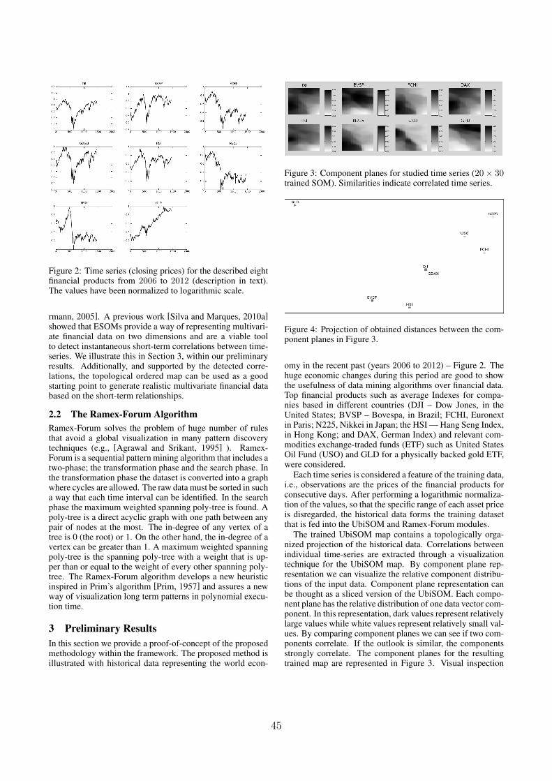
Figure 2: Time series (closing prices) for the described eightfinancial products from 2006 to 2012 (description in text).The values have been normalized to logarithmic scale.

rmann, 2005]. A previous work [Silva and Marques, 2010a]showed that ESOMs provide a way of representing multivari-ate financial data on two dimensions and are a viable toolto detect instantaneous short-term correlations between time-series. We illustrate this in Section 3, within our preliminaryresults. Additionally, and supported by the detected corre-lations, the topological ordered map can be used as a goodstarting point to generate realistic multivariate financial databased on the short-term relationships.

2.2 The Ramex-Forum AlgorithmRamex-Forum solves the problem of huge number of rulesthat avoid a global visualization in many pattern discoverytechniques (e.g., [Agrawal and Srikant, 1995] ). Ramex-Forum is a sequential pattern mining algorithm that includes atwo-phase; the transformation phase and the search phase. Inthe transformation phase the dataset is converted into a graphwhere cycles are allowed. The raw data must be sorted in sucha way that each time interval can be identified. In the searchphase the maximum weighted spanning poly-tree is found. Apoly-tree is a direct acyclic graph with one path between anypair of nodes at the most. The in-degree of any vertex of atree is 0 (the root) or 1. On the other hand, the in-degree of avertex can be greater than 1. A maximum weighted spanningpoly-tree is the spanning poly-tree with a weight that is up-per than or equal to the weight of every other spanning poly-tree. The Ramex-Forum algorithm develops a new heuristicinspired in Prim’s algorithm [Prim, 1957] and assures a newway of visualization long term patterns in polynomial execu-tion time.

3 Preliminary ResultsIn this section we provide a proof-of-concept of the proposedmethodology within the framework. The proposed method isillustrated with historical data representing the world econ-

Figure 3: Component planes for studied time series (20× 30trained SOM). Similarities indicate correlated time series.

Figure 4: Projection of obtained distances between the com-ponent planes in Figure 3.

omy in the recent past (years 2006 to 2012) – Figure 2. Thehuge economic changes during this period are good to showthe usefulness of data mining algorithms over financial data.Top financial products such as average Indexes for compa-nies based in different countries (DJI – Dow Jones, in theUnited States; BVSP – Bovespa, in Brazil; FCHI, Euronextin Paris; N225, Nikkei in Japan; the HSI — Hang Seng Index,in Hong Kong; and DAX, German Index) and relevant com-modities exchange-traded funds (ETF) such as United StatesOil Fund (USO) and GLD for a physically backed gold ETF,were considered.

Each time series is considered a feature of the training data,i.e., observations are the prices of the financial products forconsecutive days. After performing a logarithmic normaliza-tion of the values, so that the specific range of each asset priceis disregarded, the historical data forms the training datasetthat is fed into the UbiSOM and Ramex-Forum modules.

The trained UbiSOM map contains a topologically orga-nized projection of the historical data. Correlations betweenindividual time-series are extracted through a visualizationtechnique for the UbiSOM map. By component plane rep-resentation we can visualize the relative component distribu-tions of the input data. Component plane representation canbe thought as a sliced version of the UbiSOM. Each compo-nent plane has the relative distribution of one data vector com-ponent. In this representation, dark values represent relativelylarge values while white values represent relatively small val-ues. By comparing component planes we can see if two com-ponents correlate. If the outlook is similar, the componentsstrongly correlate. The component planes for the resultingtrained map are represented in Figure 3. Visual inspection

45

may suffice to detect correlations, but in [Silva and Marques,2010a] we provided an automated algorithm to cluster time-series based on a distance metric computed for pairs of com-ponent planes (Figure 4). However, this ability is only ofrelevance in this paper to justify the use of ESOM maps togenerate multivariate time-series based on a trajectory model(Section 3.1).

Figure 5 presents a Ramex-Forum generated graph for thisfinancial data, considering interactions with a latency of upto 160 (long-term) trading days over a period of 2000 days– results presented in [Marques and Cavique, 2013]. Eacharc represents the number of synchronous positive price ten-dencies (buying signals given by a moving average indica-tor). During the studied period Hong Kong HSI Index hasa behavior that was preceded by 273 times by similar vari-ations in American Dow Jones (DJI) and 179 times by Ger-man DAX. We should notice that USA DJI is influencingmost major assets in the world. The only exception to this isEuropean GermanDAX , that strongly co-influences ChineseHSI . Another correlation found is between HSI and GLDtendencies in these long term dependencies. This is some-thing that UbiSOM cannot capture and can be incorporatedwhen generating more realistic market scenarios.

3.1 Generating ScenariosBy projecting again the historical data over the UbiSOM weget a set of trajectories over the map that are used to generatethese alternate time series. A trajectory is formed by project-ing two consecutive observations from the training data andstoring the pair of neurons that were activated, in the formof a trajectory (bare in mind that loops are frequent, becausetwo similar observations are prone to be projected in the sameneuron). Figure 6 depicts these trajectories in the form of adirected graph in which each vertex represents a neuron andthe edges the obtained trajectories. The weight of the edgeindicates how many times the trajectory was followed in theprojection of the training data.

Based on this trajectory model, we can generate alternatetime series using Monte Carlo simulations. Starting at a ver-tex with edges and randomly choosing the next trajectory ofthe model to follow we can create paths of arbitrary lengths(dependent of the desired number of daily prices). Each ver-tex/neuron contains the prototype of data that contains the set

Figure 5: Correlation Ramex-Forum graph considering inter-actions with a latency of up to 160 trading days over a periodof 2000 days.

Figure 7: Simulated outcome of a possible market scenariofrom the trajectory model of a 15× 10 trained UbiSOM.

of daily prices for similar observed days. The totality of thepath then gives us the multivariate time series. Details on howto generate the path are currently being studied, it must notbe totally random, i.e., the weight on the edges must be takeninto account so as to give more importance to trajectories thatare more common. Also, when creating the trajectory modelwe store at each vertex/neuron the statistical variation of thetraining vectors that are projected on that particular neuron.This allows generating a Gaussian around each prototype vec-tor component to introduce variability on a particular virtualdaily price. This is particularly important when loops are be-ing followed in the path, so that generated time series doesn’tcontain “flat” lines.

Figure 7 depicts a sample of a generated outcome that canbe obtained from trajectories over the trained UbiSOM. It canbe seen that the multivariate time series maintain the observedcorrelations in the original historical data. This can be veryuseful in generating possible scenarios for risk estimation.

3.2 DiscussionVisual inspection of the similarity of component planes inFigure 3 shows that the results of the UbiSOM model are co-herent, e.g., DJI and DAX are strongly correlated in their his-torical behavior. GLD, as it was expected, is very far from anyother financial product. Its historical behavior is extremelydifferent in the analysis period, mainly always in a upwardmovement. All the other assets maintain a significant dis-tance from the others, showing that the correlation is not thatstrong. Interesting additional long term relations were foundby Ramex-Forum algorithm. The example shown in Figure 5,presents the USA DJI index influencing most other indexes.Also China (HSI) is detected as a major player in world econ-omy and seems to be the major influence on the price of gold(GLD). Indeed, during the analyzed period, People’s Repub-lic of China was one of the major buyers of gold in the worldand has the largest reserves of Gold and Foreign Exchange inthe world (CIA World Factbook, 2013).

However, it is the conjunction of the long term relationsdetected in Ramex-Forum with the magnitude of short timemultivariate dependencies of UbiSOM, that should be themost interesting application. Different long term trajectoriescan now be generated on the UbiSOM map, based on the longterm sequences detected by Ramex-Forum. E.g., neurons cor-

46

Figure 6: Trajectories generated for the projection of the historical training data over a 15× 10 trained UbiSOM.

47

responding to highest increases in gold values can be easilyselected from a SOM map. The same could be done for highvalues for the Chinese (HSI), or USA (DJI) economy. Highlyprobable pathways should then be made among those neu-rons. In practice these will encode the Ramex-Forum graph asa probable pathway among distinct UbiSOM neurons. Thenfor a given trading day (e.g. today) starting point, we canthen generate random walks in the map. Since each neuronrepresents a possible market state, we can easily generate foreach neuron a possible virtual trading day that is strongly re-lated with observed data. However it will be the pathwaysto provide the most interesting effect on this map. Indeed, inaverage, virtual trading days will follow possible sequencesgiven (and measured) by Ramex-Forum graph.

4 ConclusionsBoth algorithms should provide a realistic and easily usableframework to study and simulate possible effects of eithereconomic or political decisions. Even extreme events, e.g.,Acts of God, may them be given some probability. We be-lieve that such a time-series based model is a much neededtool in todays strongly interdependent and complex worldwhere over-simplistic assumptions frequently lead to poor de-cisions.

On one hand UbiSOM provides the daily correlation be-tween products and can be made self-adjustable to continu-ously changing streams of data (i.e., both collaborative learn-ing [Silva and Marques, 2010b] and detecting concept drift[Silva et al., 2012]). On the other hand Ramex-Forum graphsshows sequences of the more representative events and canbe easily used to model the dynamic of the occurrences. So,we believe that these complementary tools, one more staticand the other more dynamic, can intrinsically guarantee re-alistic modeling on different scenarios and provide a majorbreakthrough in decision support systems.

References[Agrawal and Srikant, 1995] R. Agrawal and R. Srikant.

Mining sequential patterns. In Proceedings 11th Interna-tional Conference Data Engineering, pages 3–14. IEEEPress, 1995.

[Kohonen, 1982] Teuvo Kohonen. Self-organized formationof topologically correct feature maps. Biological cyber-netics, 43(1):59–69, 1982.

[Marques and Cavique, 2013] Nuno Marques and Luis Cav-ique. Sequential pattern mining of price interactions. InProceedings 16th Portuguese Conference on Artificial In-telligence (EPIA), 2013.

[Prim, 1957] Robert Clay Prim. Shortest connection net-works and some generalizations. Bell system technicaljournal, 36(6):1389–1401, 1957.

[Silva and Marques, 2010a] B. Silva and N. Marques. Fea-ture clustering with self-organizing maps and an applica-tion to financial time series portfolio selection. In Interna-tional Conference on Neural Computation, 2010.

[Silva and Marques, 2010b] Bruno Silva and Nuno C. Mar-ques. Ubiquitous data-mining with self-organizing maps.In Proceedings of the Ubiquitous Data Mining Workshop,ECAI 2010, 2010.

[Silva et al., 2012] Bruno Silva, Nuno Marques, and GiselePanosso. Applying neural networks for concept drift de-tection in financial markets. In Workshop on UbiquitousData Mining, page 43, 2012.

[Ultsch and Herrmann, 2005] A. Ultsch and L. Herrmann.The architecture of emergent self-organizing maps to re-duce projection errors. In Proceedings of the EuropeanSymposium on Artificial Neural Networks (ESANN 2005),pages 1–6. Verleysen M. (Eds), 2005.

48

Trend template: mining trends with a semi-formal trend model

Olga Streibel, Lars Wißler, Robert Tolksdorf, Danilo Montesistreibel@inf.fu-berlin.de, lars.wissler@googlemail.com, tolk@ag-nbi.de

Networked Information Systems Group, Freie Universitat Berlin, Berlin, Germanymontesi@cs.unibo.it

University of Bologna, Bologna, Italy

AbstractPredictions of uprising or falling trends are helpfulin different scenarios in which users have to dealwith huge amount of information in a timely man-ner,such as during financial analysis. This tempo-ral aspect in various cases of data analysis requiresnovel data mining techniques. Assuming that agiven set of data, e.g. web news, contains informa-tion about a potential trend, e.g. financial crisis, itis possible to apply statistical or probabilistic meth-ods in order to find out more information about thistrend. However, we argue that in order to under-stand the context, the structure, and explanation ofa trend, it is necessary to take a knowledge-basedapproach. In our study we define trend mining andpropose the application of an ontology-based trendmodel for mining trends from textual data. We in-troduce the preliminary definition of trend miningas well as two components of our trend model: thetrend template and the trend ontology. Further-more, we discuss the results of our experimentswith trend ontology on the test corpus of Germanweb news. We show that our trend mining approachis relevant for different scenarios in ubiquitous datamining.

1 IntroductionWhen discussing trends some of us may think about the upsand downs of NASDAQ1, or DAX2 curves, or changes in pub-lic opinion on politics before elections. Likewise, one canthink about web trends, life style trends or daily trends, i.e.hot topics, in the news or on social networks. Changes in amobile data stream also fall within the definition of a trend.Understanding a trend as a hot topic is related to the researchin Emerging Topic Detection (EDT) and Topic Detection andTracking (TDT), the subfields of information retrieval [Allan,2002][Kontostathis et al., 2003]. A trend is defined there asa topic that emerges in interest and utility over time. Accord-ingly, common examples of trends may be the “Arab Spring”

1http://www.nasdaq.com/ online accessed 04-17-2013

2http://dax-indices.com/EN/index.aspx?pageID=4 online accessed 04-17-

2013

which emerged in political news worldwide in the beginningof 2011, as well as the financial and real estate crisis whichstarted to emerge on business news worldwide in 2008. Agraphical representation of a trend, based on GoogleTrends3,is shown in Fig. 1.

Figure 1: This graph shows a search volume index for the terms “fi-nancial crisis” (blue curve) and “insolvent” (red curve) in Germanyfrom 2006 to 2011. Source: GoogleTrends

Several methods have been proposed for detecting trends intexts or discovering trends in the web news (see Section 3).Other works provide approaches from statistics and time se-ries analysis that can be applied for analyzing trends in non-textual data. Our work contributes to the general understand-ing of trend mining that we see as highly relevant to ubiqui-tous data mining. In this paper, we explain our abstract con-cept of a trend template and go on to describe a trend ontologywhich is an instance of the trend template.

2 Ubiquitous data mining and trend miningThe Ubiquitous Data Mining (UDM) is defined as the essen-tial part of the ubiquitous computing [Witten and Eibe, 2005].The UDM techniques help in extracting useful knowledgefrom data that describes the world in movement, includingthe aspects of space and time. Time is the necessary dimen-sion for trend mining– there is no trend without time. And atrend is one of the aspects of a world in movement. Beforewe discuss general trend characteristics, we want to mentionthe sociological and statistical perspectives on the trend, aswell as define trend mining. This helps in understanding thetrend characteristics that create the basis for the definition ofour trend template later in this paper.

3http://www.google.com/trends/ online accessed 04-17-2013

49

2.1 Trend from different perspectivesDetecting trends from the sociological point of view is an an-alytical method for observing changes in peoples behaviorover time with regard to “six attitudes towards trends” [Ve-jlgaard, 2008]. The definition of these six attitudes is basedon eight different personality profiles of groups who partici-pate in the trend process: trend creators, trend setters, trendfollowers, early mainstreamers, mainstreamers, late main-streamers, conservatives and anti-innovators.Detecting trends from the statistics perspective is based ontrend analysis of time-series data with two goals in mind:“modeling time series (i.e. to gain insight into the mecha-nisms or underlying forces that generate the time series) andforecasting time series (i.e. to predict the future values of thetime-series variables)” [Han and Kamber, 2006]. The trendanalysis process consists of four major components: trend orlong-term movements, cyclic movements or cyclic variations,seasonal movements or seasonal variations, and irregular orrandom movements [Han and Kamber, 2006]. A trend, in thiscontext, is an indicator for a change in the data mean [Mitsa,2010].

2.2 Trend miningSince data mining can be described as “the extraction ofimplicit, previously unknown, and potentially useful infor-mation from data” [Witten and Eibe, 2005], we propose theuse of the term trend mining as defined below:

DEF 2.1 Trend mining is the extraction of implicit,previously unknown and potentially useful knowledge fromtime-ordered text or data. The trend mining techniquescan be used for capturing trend in order to support user inproviding previously unknown information and knowledgeabout the general development in users field of interests.

3 Related ResearchIn general, when mining trends from textual data, at least thefollowing three research areas should be mentioned: emer-gent trend detection, topic detection and tracking, and tem-poral data mining.In [Kontostathis et al., 2003] several systems that detectemerging trends in textual data are presented. These ETDsystems are classified into two main categories: semi-automatic and fully-automatic. For each system there is acharacterization based on the following aspects: input dataand attributes, learning algorithms and visualization. Thiscomparison includes an overview over the research publishedin [Allan et al., 1998][Lent et al., 1997][Agrawal et al.,1995][Swan and Jensen, 2000][Swan and Allan, 1999][Wattset al., 1997]. TDT research [Allan, 2002] is predomi-nantly related to the event-based approaches. Event-basedapproaches for trend mining underlie the assumption thattrends are always triggered by an event, which is often de-fined as “something happening” or “something taking place”[Lita Lundquist, 2000] in the literature. Considering a trendfrom the event research perspective means that trend detec-tion has to be understood as a monitoring task. This is mostly

the case for so-called short-term trends that are indeed trig-gered by some events and in order to detect them we haveto monitor the stream in which they occur, e.g. the occur-rence of “Eyjafjallajkull eruption”4 which was reported insocial networks and on the news in March 2010. However,so-called long-term trends, e.g. “financial crisis”, that startedto be on-topic in 2008 are not necessarily conjoined with onespecific event. It is more a chain of events or even the “soft”indicators as public opinion or news. No sharp distinctionhas been made between the TDT and ETD research fields,which means that some research such as [Swan and Allan,1999] or [Lavrenko et al., 2000] can be in fact classified intoboth fields. Temporal data mining research [Mitsa, 2010] of-fers methods for clustering, classification, dimension reduc-tion and processing of time-series data [Wang et al., 2005].It addresses in general the temporal data and the techniquesof time series analysis on these data. One definition of tem-poral data is “time series data which consist of real valuedsampled at regular time intervals” [Mitsa, 2010]. Temporaldata mining applies the data mining methodology and dealswith the same approaches for classification or clustering, thatare relevant for mining trends in textual data.

4 Trend templateBased on our experiments and considerations, we outline thefollowing assumptions about trends in the general context ofthis work;A trend can be described by the following characteristics:trigger, context, amplitude, direction, time interval, and re-lation. Fig. 2 illustrates the trend template.In 4.1, we more precisely define each characteristic.

4.1 DefinitionsTrigger is a thing. They can be: an event, a person, or a topicanything that triggers the trend. A trigger can but does nothave to cause a trend. A trigger makes the trend visible. Anexample of a trigger is Lehman Brothers5 insolvency that canbe classified as both a topic and an event.Context is the area of the trigger. If the trigger is a topicthen the context is this topic’s area, e.g. Lehman Brothersinsolvency is mentioned in the context of real estate market.Amplitude is the strength of a given trend. It can beexpressed by a number, the higher the number the moreimpact the trend has or by a qualitative value that describesthe trend phase, e.g. beginning (setter), emerging (follower),mainstream, fading (conservative).Time is necessary while spotting trend, since there can beno trend without time. It is the interval in which the trendis appearing, independent from the amplitude, e.g. the realestate crisis appeared between the years 2008-2011.Relation expresses the dependency between the trigger andthe context, it puts the given trigger, e.g. Lehman Brothersinsolvency within the given context of the real estate crisisin a relation, e.g. Lehman Brothers insolvency is part of the

4The eruption of an Icelandic volcano in March 2010 that caused air travel chaos in Eu-

rope and revenue lost for the airlines http://www.volcanodiscovery.com/iceland/eyjafjallajoekull.html online accessed 04-17-2013

5http://www.lehman.com/ online accessed 04-17-2013

50

Figure 2: Trend template– an abstract conceptualization

real estate crisis.

4.2 Formal descriptionThe trend template is an abstract model that describesthe main concepts that are important and necessary forknowledge-based trend mining. In following, we more ex-plicitly define the trend template:DEF. 4.1: Trend template (TT) is a quintuple:

TT := 〈T,C,R, TW,A〉where: T is trigger, C is context, R is relation, TW is timewindow, and A is amplitude.

DEF. 4.2: T- Trigger is set of concepts:

T := {t0, . . . , tn}, n ∈ N ∧ t ∈ Tso that if E, P , To are the sets defining:events: E := {e0, . . . , en}, n ∈ N ∧ e ∈ Epersons: P := {p0, . . . , pn}, n ∈ N ∧ p ∈ Plocations: L := {l0, . . . , ln}, n ∈ N ∧ l ∈ Ltopics: To := {to0, . . . , ton}, n ∈ N ∧ to ∈ Tothen:

T := E ∪ P ∪ To ∪ LDEF. 4.3: C- Context is a union set consisting of a set ofconcepts and a set of relations between them where c is acontext element:

C := Cco ∪Rco, c ∈ Cwith Cco the set of concepts

Cco := {cco0, . . . , ccon}, n ∈ N ∧ cco ∈ Cco

and Rco the set of relations:

Rco := {rco0, . . . , rcon}, n ∈ N∧rco ∈ Rco∧Rco ⊆ Cco × Cco

whereas rco defines a binary relation:

rco : ccox, ccoy −→ rco(ccox, ccoy) ∧ ccox 6= ccoy

and the context element is defined by:

c = cco ∪ (ccoi, ccoj)

C = Cco ∪ Cco × Cco

DEF. 4.4: R-Relational is a set of relations:

R := {r0, . . . , rn}, n ∈ N ∧ r ∈ R ∧R := {T × C}with

ri : ti, ci −→ ri(ti, ci)

DEF. 4.5: TW- Time window is a function that assigns timeslice to the time points:

TP := {tpoint|tpoint == ms ∨ second ∨minute ∨ hour ∨ day ∨month ∨ year}

TS := 〈tpoint0 . . . tpointn〉TW : TP −→ TS

DEF. 4.6: A- Amplitude is a function that assigns a value tothe quadruple of 〈T,C,R, TW 〉

A : T × C ×R× TW −→ N ∪ Vwhere N is the set of natural numbers and V is the set ofcategorical values

a : (t, c, r, tw) −→ n ∨ v

51

5 Trend OntologyOne way of implementing the trend template is the realizationof this model in the form of an ontology. We can understandthe ontology as an instance of the trend template.

Based on the trend template described above, we created anapplicable model, using SKOS6 and RDFS/OWL7 conceptsand properties. Our model serves as a general model thatcan be extended regarding the particular application domainand applied for annotating a text corpus in order to retrievethe trend structure. The trend ontology is divided into levelsmeta, middle and low which correspond to three abstract lay-ers of the model. Whereas the low level and the middle levelrelate to the corresponding application domain (in our case itis the German Stock Exchange, DAX), the meta level is themost interesting one. Meta ontology incorporates the generaltrend characteristics and can be applied to any application do-main.The central concepts of the ontology are Trigger, Trig-gerCollection, Indication, Relational and ValuePartitionand have been modeled as subconcepts of skos:Concept,skos:Collection and time:TemporalEntity, with different se-mantic construction, e.g. skos:related, skos:member. Theconcepts mirror the composition of the trend template. Trig-ger consists of three subconcepts: event, person, location.The main goal of the meta ontology is to offer all necessaryconcepts and relations in order to span the trend template asa structure over a text corpus. To actually translate a specificdocument corpus into such a structure, meta ontology needsto be combined with a domain specific trend ontology whichdefines domain specific concepts, their keywords and possi-bly also their relations. This can either be done manually byextracting common terms as keywords and linking them totheir respective concepts, or automatically by entity recog-nition. The pseudocode 6.1 describes the algorithm that weapplied to build up the trend description on the test corpus.

6 ExperimentsThe text corpus which we call German finance data8 thatserved as our test corpus consists of about 40,500 news ar-ticles related to the fields of business and finance, providedas XML files. The corpus is available in German and pro-vides news articles from January 2007 to May 2008. The textwas parsed in cooperation with neofonie9 from the followingsources: comdirect10, derivatecheck11, Handelsblatt12, God-modeTrader13, Yahoo14, Financial Times Deutschland15, andfinanzen.net16.

6http://www.w3.org/2004/02/skos/ online accessed 04-17-2013

7http://www.w3.org/TR/owl-features/ online accessed 04-17-2013

8Currently (May 2013) in the publishing process at Linguistic Data Consortium http://www.

ldc.upenn.edu/9http://www.neofonie.de, online accessed 04-25-2012

10http://www.comdirect.de/inf/index.html, online accessed 04-25-2012

11http://derivatecheck.de/, online accessed 04-25-2012

12http://www.handelsblatt.com/weblogs/, online accessed 04-25-2012

13http://www.godmode-trader.de/, online accessed 04-25-2012

14http://de.biz.yahoo.com/, online accessed 04-25-2012

15http://www.ftd.de/, online accessed 04-25-2012

16http://www.finanzen.net, online accessed 04-30-2012

Algorithm6.1: CREATETRENDDESCRIPTION(c, o)

comment: parse ∀ document ∈ corpus

comment: into ontology

parse(c, inO, outO){model.read(inO)create.reasoner(inO)for each d∈ c

do {parse(keywords);match.model(keywords, inO){for keyword← 0 to iif inO.concept.label==keyword orkeyword∈ inO.concept.labelkeyword.prefix or keyword.postfix==inO.concept.label.prefix or .postfix

then matches.add(keyword)}relate.model(matches, inO){if model.getRelation(matches).isEmpty

then model.createRelation(matches)else model.incCounter(matches)}}

model.write(outO)

In general, the content of the corpus is focused on financeand business information concerning German companies andstocks. It focuses on the situation at DAX, as well as on re-views and ratings of German companies and shares. For eval-uation purposes regarding usefulness and practicability, thetrend ontology has been filled with two different parts of thetest corpus: stock market specific documents in Part 1 and thegeneral business news in Part 2 (subsequently first and secondpart). They contain over 5,000 and 16,000 documents respec-tively. We specified several basic questions and respectivequeries as relevant for trends in general and specifically forstock market trends. Querying the ontology for the total oc-currence of concepts yields the following output (shortened tosome of the most relevant concepts): Germany (9,137), USA(4,808), Deutsche Telekom (442), Allianz (433), Switzerland(382), Starbucks (104). The output corresponds directly tothe corpus of German stock news with a clear focus on Ger-man companies followed by the still dominant US market. Asimilar query for often mentioned lines of business in the con-text of Germany in contrast to the USA yields a major focuson the industry for Germany. 4.5% to 7.1% of the total oc-currences of Germany appear in the context of different linesof industry. The USA is strong in the context of IT (9%) andservices (6.9%). Moreover, we checked so-called topic struc-ture by using our ontology. Here a general example for theconcept Germany:

trendonto:#Germany (9137) has Topictrendonto:#Financial : 1142trendonto:#buy : 1003trendonto:#MachineBuildingIndustry : 650trendonto:#Share : 606trendonto:#StockPrice : 562trendonto:#Up : 520trendonto:#Industry : 510trendonto:#Investment : 468trendonto:#Supplier : 422trendonto:#AutomobilIndustry : 414

52

Figure 3: Performance of shares in the first corpus (5,000 docu-ments) by ontology based ranking and comparison with share in-dices in the time window July 2007 to July 2011.

In Fig. 3 we show the comparison of the performance val-ues for the stock markets as ranked by ontology (test based ontime window: July 2007 to April 2008) and reported in real(time window July 2007 to July 2011). Applying the trendontology to the test set enables to find out specific informa-tion about the certain trend that is described in the documentsof the test set. Our preliminary experiments results that wepartially present in this paper show that our idea of a trendtemplate could help in harvesting knowledge from the giventest data in a timely manner.

7 Conclusions and future workThis paper presents our research on knowledge-based trendmining, wherein the main contribution is our semi-formalmodel of a trend template. We showed that the implemen-tation of the trend template in the form of a trend ontologyallows for capturing the trend structure out of a test docu-ment set. Our experiments confirm that a knowledge-basedapproach for mining trends out of data allows for extendedtrend explanations. Currently we are comparing the trend on-tology experiment results with the results from adapted K-Means clustering and LDA-based topic modeling algorithmsapplied on our test set.

AcknowledgmentsThis work has been partially supported by the “InnoProfile-Corporate Semantic Web” project funded by the German Fed-eral Ministry of Education and Research (BMBF) and theBMBF Innovation Initiative for the New German Lander -Entrepreneurial Regions.

References[Agrawal et al., 1995] Rakesh Agrawal, Edward L. Wim-

mers, and Mohamed Zait. Querying shapes of histories.In Proceedings of the 21st VLDB, pages 502–514. MorganKaufmann Publishers Inc., 1995.

[Allan et al., 1998] James Allan, Ron Papka, and VictorLavrenko. On-line new event detection and tracking. InSIGIR’98: Proceedings of the 21st annual international

ACM SIGIR conference on Research and development ininformation retrieval, pages 37–45. ACM, 1998.

[Allan, 2002] James Allan, editor. Topic Detection andTracking. Event-based Information Organization. Kluweracademic publishers, 2002.

[Han and Kamber, 2006] J. Han and M. Kamber. Data Min-ing Concepts and Techniques. Morgan Kaufmann Publish-ers Inc., 2006.

[Kontostathis et al., 2003] April Kontostathis, Leon Galit-sky, William M. Pottenger, Soma Roy, and Daniel J.Phelps. A Survey of Emerging Trend Detection in TextualData Mining. Springer-Verlag, 2003.

[Lavrenko et al., 2000] Victor Lavrenko, Matt Schmill,Dawn Lawrie, Paul Ogilvie, David Jensen, and JamesAllan. Mining of concurrent text and time series. InProceedings of the 6 th ACM SIGKDD InternationalConference on Knowledge Discovery and Data MiningWorkshop on Text Mining, pages 37–44, 2000.

[Lent et al., 1997] Brian Lent, Rakesh Agrawal, and Ra-makrishnan Srikant. Discovering trends in text databases.In Proceedings of the KDD’97, pages 227–230. AAAIPress, 1997.

[Lita Lundquist, 2000] Robert J. Jarvella Lita Lundquist.Language, Text, and Knowledge. Mental Models of ExpertCommunication. De Gruyter, 2000.

[Mitsa, 2010] Theophano Mitsa, editor. Temporal Data Min-ing. Chapman Hall/CRC Press, 2010.

[Swan and Allan, 1999] Russell Swan and James Allan. Ex-tracting significant time varying features from text. InCIKM’99: Proceedings of the eighth international confer-ence on Information and knowledge management, pages38–45. ACM, 1999.

[Swan and Jensen, 2000] Russel Swan and David Jensen.Timemines: Constructing timelines with statistical modelsof word usage. In KDD-2000 Workshop on Text Mining,2000.

[Vejlgaard, 2008] Henrik Vejlgaard. Anatomy of A Trend.McGraw-Hill, 2008.

[Wang et al., 2005] X. Wang, K. Smith, and R. Hyndman.Dimension reduction for clustering time series usingglobal characteristics. In Vaidy Sunderam, Geert van Al-bada, Peter Sloot, and Jack Dongarra, editors, Computa-tional Science - ICCS 2005, volume 3516 of Lecture Notesin Computer Science, pages 11–14. Springer Berlin / Hei-delberg, 2005.

[Watts et al., 1997] Robert J. Watts, Alan L. Porter, ScottCunningham, and Donghua Zhu. Toas intelligence min-ing; analysis of natural language processing and computa-tional linguistics. In PKDD ’97: Proceedings of the FirstEuropean Symposium on Principles of Data Mining andKnowledge Discovery, pages 323–334. Springer-Verlag,1997.

[Witten and Eibe, 2005] Ian. H. Witten and F. Eibe. DataMining Concepts and Techniques. Morgan KaufmannPublishers Inc, 2005.

53

Ubiquitous Self-Organizing Maps

Bruno SilvaDSI/ESTSetubal

Instituto Politecnico de SetubalPortugal

bruno.silva@estsetubal.ips.pt

Nuno MarquesDI/FCT - UNL

Portugalnmm@di.fct.unl.pt

Knowledge discovery in ubiquitous environments are usu-ally conditioned by the data stream model, e.g., data is poten-tially infinite, arrives continuously and is subject to conceptdrift. These factors present additional challenges to standarddata mining algorithms. Artificial Neural Networks (ANN)models are still poorly explored in these settings.

State-of-the-art methods to deal with data streams aresingle-pass modifications of standard algorithms, e.g., K-means for clustering, and involve some relaxation of the qual-ity of the results, i.e., since the data cannot be revisited to re-fine the models, the goal is to achieve good approximations[Gama, 2010]. In [Guha et al., 2003] an improved single passk-means algorithm is proposed. However, k-means suffersfrom the problem that the initial k clusters have to be set eitherrandomly or through other methods. This has a strong impacton the quality of the clustering process. CluStream [Aggar-wal et al., 2003] is a framework that targets high-dimensionaldata streams in a two-phased approach, where an online phaseproduces micro-clusterings of the incoming data, while pro-ducing on-demand offline models of data also with k-means.

In this position paper we address the use of Self-Organizing Maps (SOM) [Kohonen, 1982] and argue itsstrengths over current methods and directions to be exploredon its adaptation to ubiquitous environments, which involvedynamic estimation of the learning parameters based on mea-suring concept drift on, usually, non-stationary underlyingdistributions. In a previous work [Silva and Marques, 2012]we presented a neural network-based framework for datastream mining that explored the two-phased methodology,where the SOM produced offline models. In this paper weadvocate the development of a standalone Ubiquitous SOM(UbiSOM), that is capable of producing models in an onlinefashion, to be integrated in the framework. This allows de-rived knowledge to be accessible at any time.

The Self-Organizing Map is a well-established data-mining algorithm with hundreds of applications throughoutenumerate scientific domains for tasks of classification, clus-tering and detection of non-linear relationships between fea-tures [Oja et al., 2003]. It can be visualized as a sheet-like neural-network array, whose neurons become specificallytuned to various input vectors (observations) in an orderlyfashion. The SOM is able to project high-dimensional dataonto a 2D lattice, while preserving topological relationships

among the input data, thus electing it as a data-mining tool ofchoice [Vesanto, 1999], either for clustering, data inspectionand/or classification. The powerful visualization techniquesfor SOM models allow the detection of complex cluster struc-tures, detection of non-linear relationships between featuresand even allow the clustering of time series.

As with most standard data mining methods, classicalSOM training algorithms are tailored to revisit the data sev-eral times to build good models. As training progresses, ex-isting learning parameters are decreased monotonically overtime through one of a variety of decreasing functions. Thisis required for the network to converge to a topological or-dered state and to estimate the input space density. The con-sequence is that the maps lose plasticity over time, i.e., if atraining sample presented at a later point in time is very dif-ferent from what it has learned so far it does not have theability to represent this new data appropriately because theseparameters do not allow large updates at that time. In ubiqui-tous environments data is expected to be presented to the net-work over time, i.e., the network should be learning graduallyand derived knowledge should be accessible at any time. Thismeans that the SOM must be able to retain an indefinite plas-ticity over time, with the ability to incorporate very differentdata from what it has learned at a particular time, i.e., to be inconformance with the “dynamic environment” requirement.

Ubiquitous SOMs , i.e., self-organizing maps tailored forubiquitous environments with streaming data, should definethose parameters not based on time t, but in the error on thenetwork for a particular observation.

An underused variant of the SOM, called the parameter-less SOM (PLSOM) [Berglund, 2010]), was first introducedto address the difficulty os estimating the initial learning pa-rameters. The PLSOM has only one parameter β (neighbor-hood range) that needs to be specified in the beginning of thetraining process, after which α (learning rate) and σ (neigh-borhood radius) are estimated dynamically at each iteration.The basic idea behind the PLSOM is that for an input pat-tern that the network already represents well, there is no needfor large adjustments – learning rate and neighborhood radiusare kept small. On the other hand, if an input vector is verydissimilar of what was seen previously, then those parame-ters are adjusted to produce large adjustments. However, inits current form, it fails in mapping the input space density

54

Figure 1: Learned Gaussian distribution for the classicalSOM (left) and for the PLSOM (right). The later does notmaintain the density of the input space, which underminesthe use of visualization techniques for cluster detection andfeature correlation.

onto the 2D lattice (Figure 1). This undermines the visual-ization capabilities of the PLSOM, namely for cluster detec-tion. Also, by estimating the values of the learning parame-ters solely based on the network error for a given observation,it is very sensible to outliers.

Nevertheless, this variant of the SOM retains an indefiniteplasticity, which allows the SOM to react to very different in-put samples from what has been presented to it, at any pointin time; and converges faster to an initial global ordered stateof the lattice. These two capabilities makes PLSOM an inter-esting starting point for the proposed goal.

Concept drift means that the concept about which data isbeing collected may shift from time to time, each time aftersome minimum permanence. Changes occur over time. Theevidence of drift in a concept is reflected in the training sam-ples (e.g., change of mean, variance and/or correlation). Oldobservations, which reflect the behavior in nature in the past,become irrelevant to the current state of the phenomena un-der observation [Gama, 2010]. In [Silva et al., 2012] we ad-dressed concept drift detection using a different type of neu-ral network, namely Adaptive Resonance Theory (ART) net-works. Figure 2 illustrates its applicability to financial timeseries. It works by measuring the quantization error of the lastbuilt micro-cluster ART model, over a predefined number ofprevious ones. We propose to use the ideas of the PLSOMalgorithm using the network error as an input to a conceptdrift module, either ANN-based or not. While the concept isstable, the learning parameters are being decreased monoton-ically so as to map the input space density; when the conceptbegins to drift the parameters are adjusted to higher values soas to cope with the different observations. If the, possibly, un-derlying non-stationary distribution is drifting rapidly, main-taining higher learning parameters will, consequently, makethe model “forget” old and irrelevant observations to the cur-rent state.

Conclusion ANN methods exhibit some advantages inubiquitous data mining: they have the ability to adapt tochanging environments; have the ability to generalize fromwhat they have learned; and through the ANN error it is pos-sible to determine if the new information that arrives is very

Figure 2: a) Measuring concept drift over a stream of finan-cial statistical indicators in [Silva et al., 2012]. b) The corre-sponding time series of the Dow Jones Index.

different from what it has learned so far. A purely onlineUbiquitous Self-Organizing Map (UbiSOM) that can learnnon-stationary distributions is relevant for data stream min-ing, namely because of its c. The SOM mining capabilitiesgreatly surpass K-means, without introducing a big overheadin computation needs. Measuring concept drift as a way toestimate the learning parameters of the learning algorithm is,in our belief, a promising path.

References[Aggarwal et al., 2003] C.C. Aggarwal, J. Han, J. Wang, and

P.S. Yu. A framework for clustering evolving data streams.In VLDB, pages 81–92, 2003.

[Berglund, 2010] E. Berglund. Improved PLSOM algorithm.Applied Intelligence, 32(1):122–130, 2010.

[Gama, 2010] Joao Gama. Knowledge discovery from datastreams. Chapman & Hall/CRC Data Mining and Knowl-edge Discovery Series, 2010.

[Guha et al., 2003] S. Guha, A. Meyerson, N. Mishra,R. Motwani, and L. O’Callaghan. Clustering data streams:Theory and practice. IEEE Transactions on Knowledgeand Data Engineering, pages 515–528, 2003.

[Kohonen, 1982] T. Kohonen. Self-organized formation oftopologically correct feature maps. Biological cybernetics,43(1):59–69, 1982.

[Oja et al., 2003] Merja Oja, Samuel Kaski, and Teuvo Ko-honen. Bibliography of self-organizing map (som) papers:1998-2001, 2003.

[Silva and Marques, 2012] Bruno Silva and Nuno Marques.Neural network-based framework for data stream mining.In Proceedings of the Sixth Starting AI Researchers’ Sym-posium. IOS Press, 2012.

[Silva et al., 2012] Bruno Silva, Nuno Marques, and GiselePanosso. Applying neural networks for concept drift de-tection in financial markets. In ECAI2012, UbiquitousData Mining Workshop, 2012.

[Vesanto, 1999] J. Vesanto. SOM-based data visualizationmethods. Intelligent-Data-Analysis, 3:111–26, 1999.

55