Workshop ITG-Fachgruppe 5.3.1 Simulation and … · Multicore fiber: a fiber-cladding structure...

Chair for Communications

Kiel University

Christian-Albrechts Universität zu Kiel, Germany

Carlos Castro, Klaus Pulverer, Stefano Calabrò, Marc Bohn, and Werner Rosenkranz

Workshop ITG-Fachgruppe 5.3.1

Simulation and Experimental Verification of a Multicore Fiber System

February 2017

-2-Chair for Communications

Kiel University

C. Castro. 16-02-2017

[email protected]@tf.uni-kiel.de

Outline

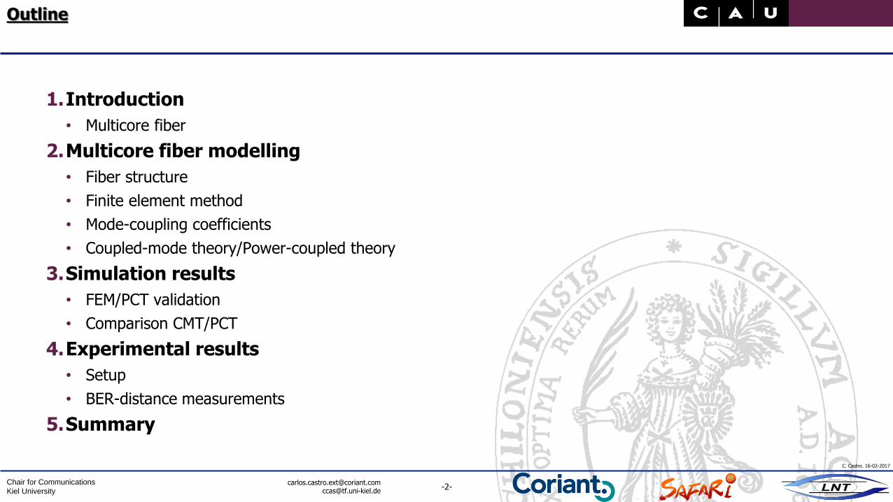
1.Introduction

• Multicore fiber

2.Multicore fiber modelling

• Fiber structure

• Finite element method

• Mode-coupling coefficients

• Coupled-mode theory/Power-coupled theory

3.Simulation results

• FEM/PCT validation

• Comparison CMT/PCT

4.Experimental results

• Setup

• BER-distance measurements

5.Summary


Kiel University

C. Castro. 16-02-2017


Introduction

Multicore fiber

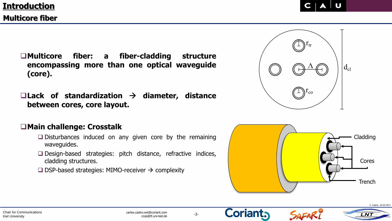
Multicore fiber: a fiber-cladding structureencompassing more than one optical waveguide(core).

Lack of standardization diameter, distance

between cores, core layout.

Main challenge: Crosstalk

Disturbances induced on any given core by the remainingwaveguides.

Design-based strategies: pitch distance, refractive indices,cladding structures.

DSP-based strategies: MIMO-receiver complexity

Cladding

Cores

Trench


Kiel University

C. Castro. 16-02-2017


Multicore fiber modelling

Fiber structure

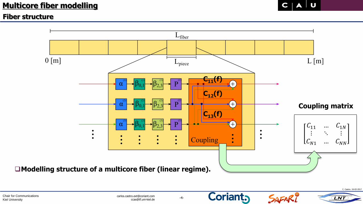
Modelling structure of a multicore fiber (linear regime).

C11(f)

C12(f)

C13(f)

𝐶11 … 𝐶1𝑁⋮ ⋱ ⋮𝐶𝑁1 … 𝐶𝑁𝑁

Coupling matrix


Kiel University

C. Castro. 16-02-2017



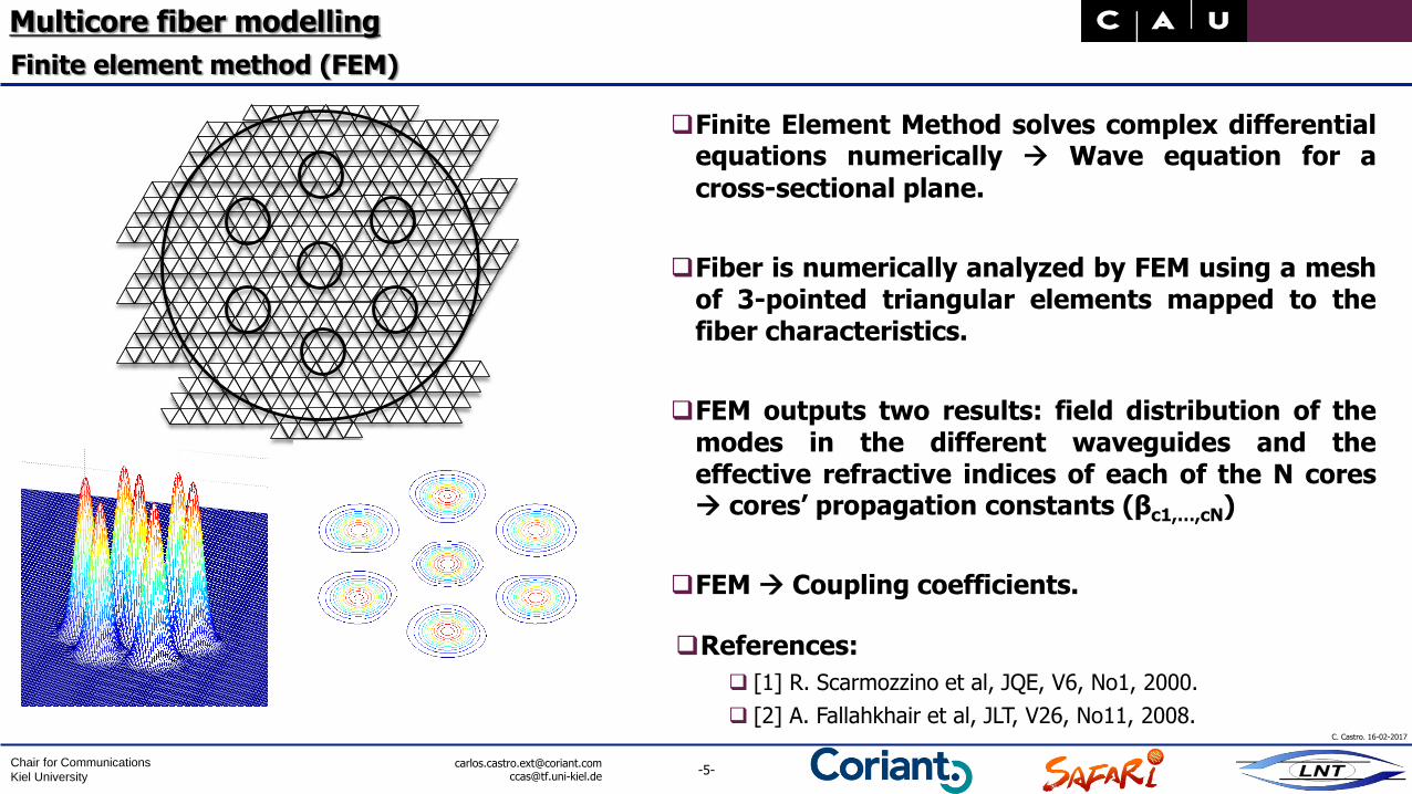
Finite element method (FEM)

Finite Element Method solves complex differentialequations numerically Wave equation for a

cross-sectional plane.

Fiber is numerically analyzed by FEM using a meshof 3-pointed triangular elements mapped to thefiber characteristics.

FEM outputs two results: field distribution of themodes in the different waveguides and theeffective refractive indices of each of the N cores cores’ propagation constants (βc1,…,cN)

FEM Coupling coefficients.

References:

[1] R. Scarmozzino et al, JQE, V6, No1, 2000.

[2] A. Fallahkhair et al, JLT, V26, No11, 2008.


Kiel University

C. Castro. 16-02-2017



Mode coupling coefficients

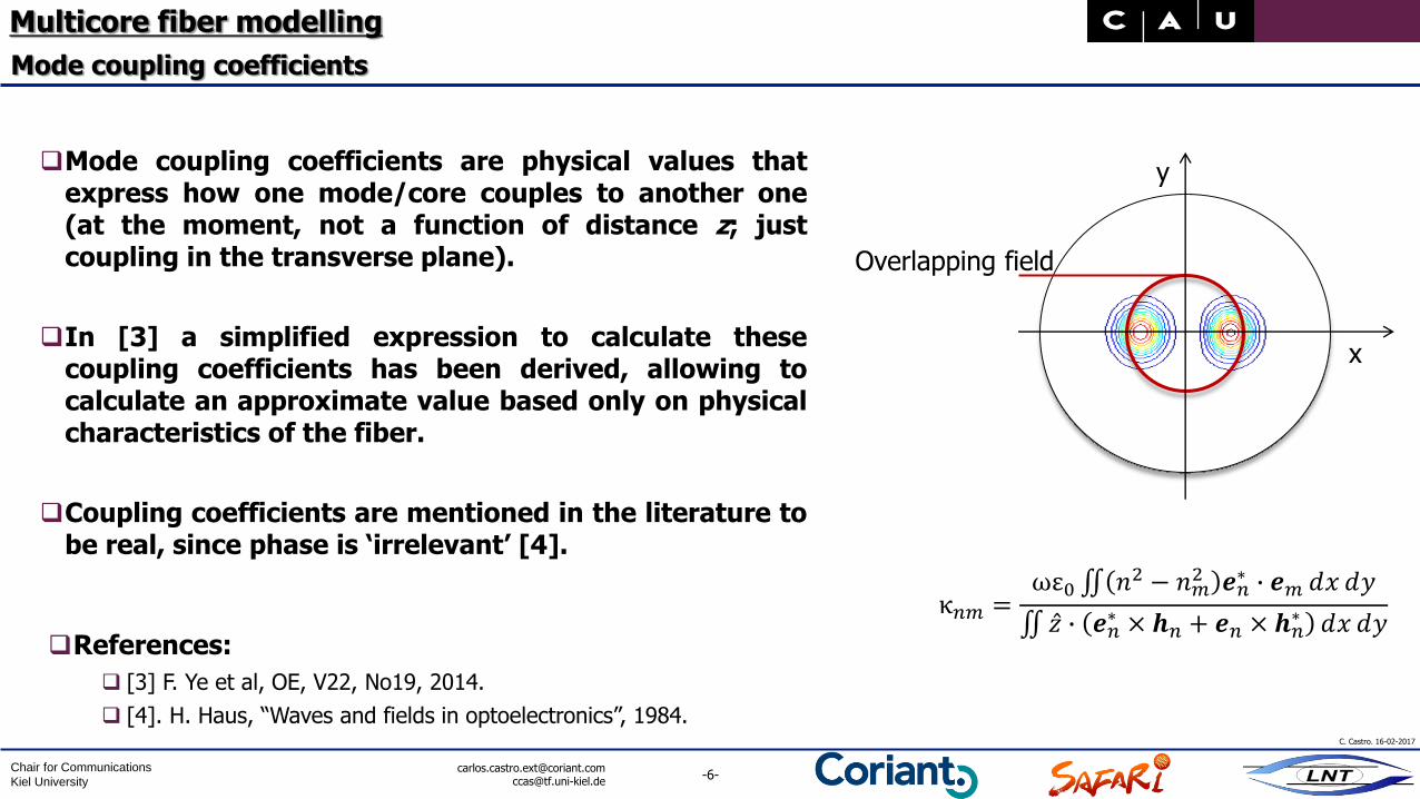
Mode coupling coefficients are physical values thatexpress how one mode/core couples to another one(at the moment, not a function of distance z; justcoupling in the transverse plane).

In [3] a simplified expression to calculate thesecoupling coefficients has been derived, allowing tocalculate an approximate value based only on physicalcharacteristics of the fiber.

Coupling coefficients are mentioned in the literature tobe real, since phase is ‘irrelevant’ [4].

Overlapping field

x

y

κ𝑛𝑚 =ωε0 𝑛

2 − 𝑛𝑚2 𝒆𝑛∗ ∙ 𝒆𝑚 ⅆ𝑥 ⅆ𝑦

𝑧 ∙ 𝒆𝑛∗ × 𝒉𝑛 + 𝒆𝑛 × 𝒉𝑛

∗ ⅆ𝑥 ⅆ𝑦References:

[3] F. Ye et al, OE, V22, No19, 2014.

[4]. H. Haus, “Waves and fields in optoelectronics”, 1984.


Kiel University

C. Castro. 16-02-2017



Coupled Mode Theory (CMT)

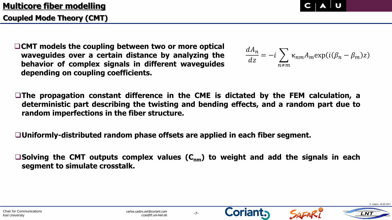
CMT models the coupling between two or more opticalwaveguides over a certain distance by analyzing thebehavior of complex signals in different waveguidesdepending on coupling coefficients.

ⅆ𝐴𝑛ⅆ𝑧= −𝑖

𝑛≠𝑚

κ𝑛𝑚𝐴𝑚exp 𝑖 𝛽𝑛 − 𝛽𝑚 𝑧

The propagation constant difference in the CME is dictated by the FEM calculation, adeterministic part describing the twisting and bending effects, and a random part due torandom imperfections in the fiber structure.

Uniformly-distributed random phase offsets are applied in each fiber segment.

Solving the CMT outputs complex values (Cnm) to weight and add the signals in eachsegment to simulate crosstalk.


Kiel University

C. Castro. 16-02-2017



Power Coupled Theory (PCT)

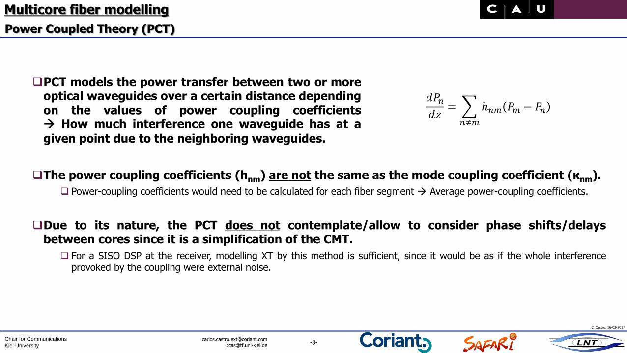
PCT models the power transfer between two or moreoptical waveguides over a certain distance dependingon the values of power coupling coefficients How much interference one waveguide has at a

given point due to the neighboring waveguides.

ⅆ𝑃𝑛ⅆ𝑧=

𝑛≠𝑚

ℎ𝑛𝑚 𝑃𝑚 − 𝑃𝑛

The power coupling coefficients (hnm) are not the same as the mode coupling coefficient (κnm).

Power-coupling coefficients would need to be calculated for each fiber segment Average power-coupling coefficients.

Due to its nature, the PCT does not contemplate/allow to consider phase shifts/delaysbetween cores since it is a simplification of the CMT.

For a SISO DSP at the receiver, modelling XT by this method is sufficient, since it would be as if the whole interferenceprovoked by the coupling were external noise.


Kiel University

C. Castro. 16-02-2017


Simulation results

FEM/PCT validation

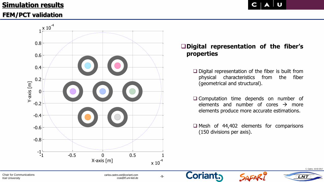
Digital representation of the fiber’sproperties

Digital representation of the fiber is built fromphysical characteristics from the fiber(geometrical and structural).

Computation time depends on number ofelements and number of cores more

elements produce more accurate estimations.

Mesh of 44,402 elements for comparisons(150 divisions per axis).

-1 -0.5 0 0.5 1

x 10-4

-1

-0.8

-0.6

-0.4

-0.2

0

0.2

0.4

0.6

0.8

1x 10

-4

X-axis [m]

Y-a

xis

[m

]


Kiel University

C. Castro. 16-02-2017


Simulation results

FEM/PCT validation

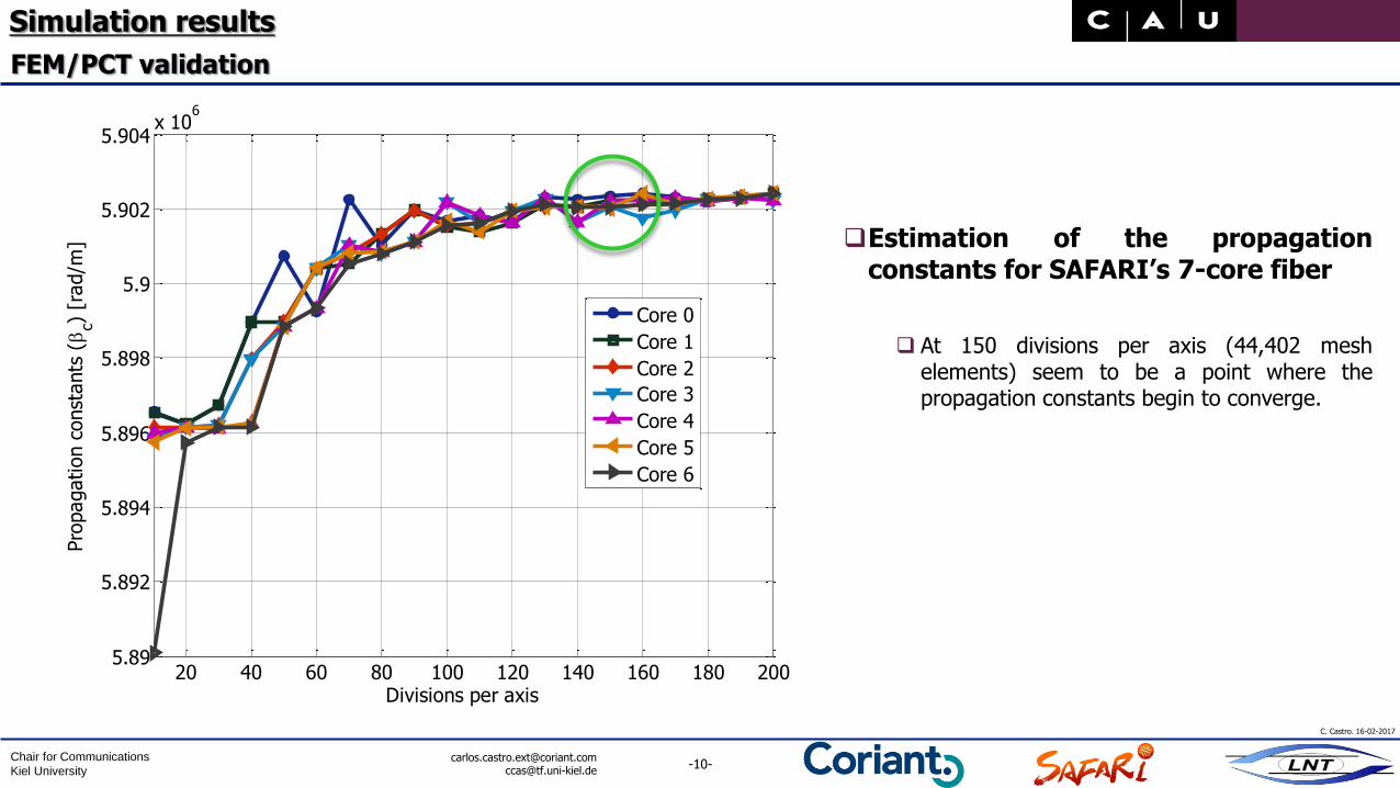
Estimation of the propagationconstants for SAFARI’s 7-core fiber

At 150 divisions per axis (44,402 meshelements) seem to be a point where thepropagation constants begin to converge.

20 40 60 80 100 120 140 160 180 2005.89

5.892

5.894

5.896

5.898

5.9

5.902

5.904x 10

6

Divisions per axis

Pro

pagation c

onst

ants

(

c) [r

ad/m

]

Core 0

Core 1

Core 2

Core 3

Core 4

Core 5

Core 6


Kiel University

C. Castro. 16-02-2017


Simulation results

FEM/PCT validation

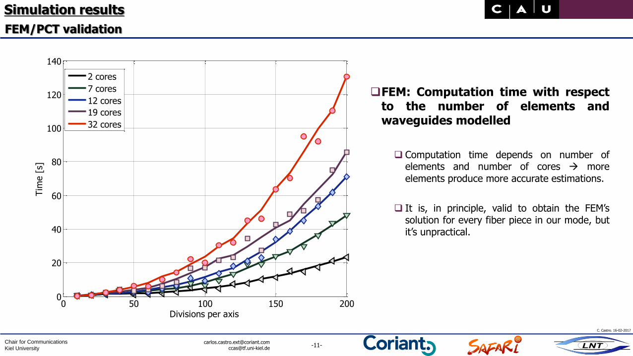
FEM: Computation time with respectto the number of elements andwaveguides modelled

Computation time depends on number ofelements and number of cores more

elements produce more accurate estimations.

It is, in principle, valid to obtain the FEM’ssolution for every fiber piece in our mode, butit’s unpractical.

0 50 100 150 2000

20

40

60

80

100

120

140

Divisions per axis

Tim

e [

s]

2 cores

7 cores

12 cores

19 cores

32 cores


Kiel University

C. Castro. 16-02-2017


Simulation results

FEM/PCT validation

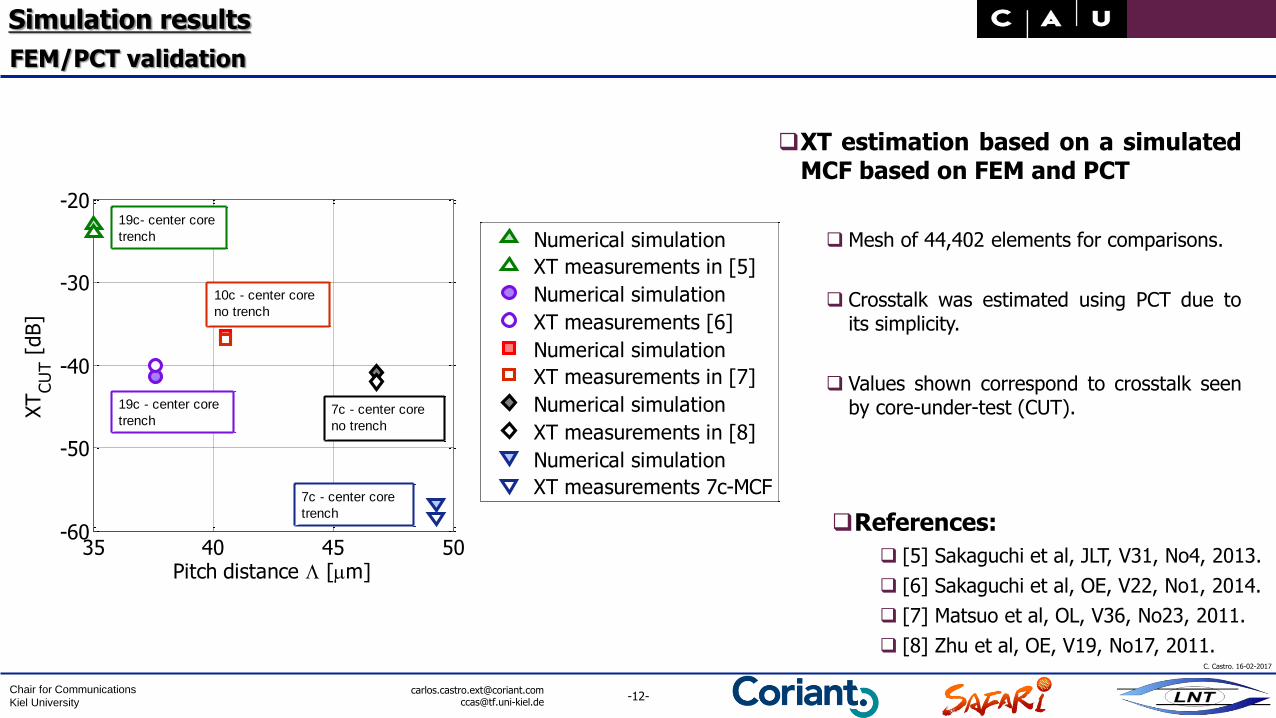
XT estimation based on a simulatedMCF based on FEM and PCT

Mesh of 44,402 elements for comparisons.

Crosstalk was estimated using PCT due toits simplicity.

Values shown correspond to crosstalk seenby core-under-test (CUT).

References:

[5] Sakaguchi et al, JLT, V31, No4, 2013.

[6] Sakaguchi et al, OE, V22, No1, 2014.

[7] Matsuo et al, OL, V36, No23, 2011.

[8] Zhu et al, OE, V19, No17, 2011.

35 40 45 50-60

-50

-40

-30

-20

Pitch distance [m]

XT

CU

T [

dB]

Numerical simulation

XT measurements in [5]


XT measurements [6]






XT measurements 7c-MCF

10c - center core

no trench

7c - center core

no trench

19c- center core

trench

19c - center core

trench

7c - center core

trench


Kiel University

C. Castro. 16-02-2017


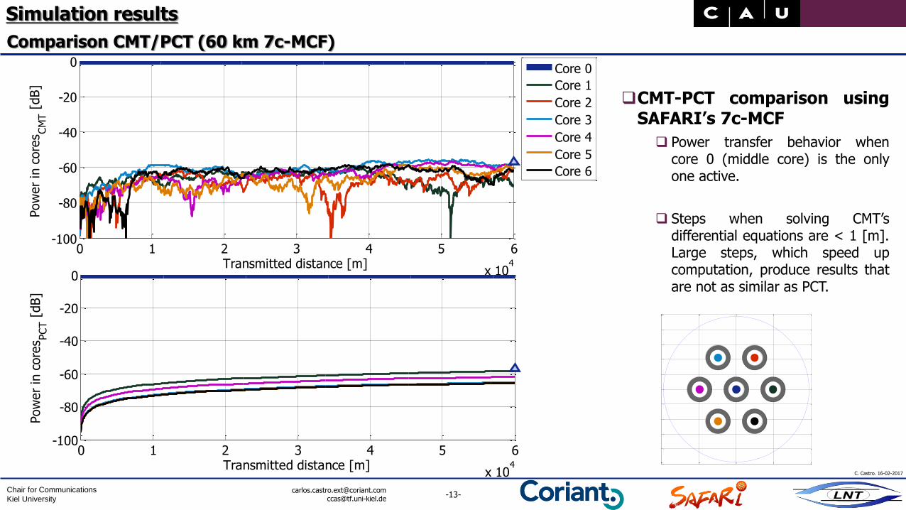
Simulation results

Comparison CMT/PCT (60 km 7c-MCF)

CMT-PCT comparison usingSAFARI’s 7c-MCF

Power transfer behavior whencore 0 (middle core) is the onlyone active.

Steps when solving CMT’sdifferential equations are < 1 [m].Large steps, which speed upcomputation, produce results thatare not as similar as PCT.

0 1 2 3 4 5 6

x 104

-100

-80

-60

-40

-20

0

Transmitted distance [m]

Pow

er

in c

ore

s CM

T [

dB]

Core 0

Core 1

Core 2

Core 3

Core 4

Core 5

Core 6

0 1 2 3 4 5 6

x 104

-100

-80

-60

-40

-20

0


Pow

er

in c

ore

s PCT [

dB]


Kiel University

C. Castro. 16-02-2017


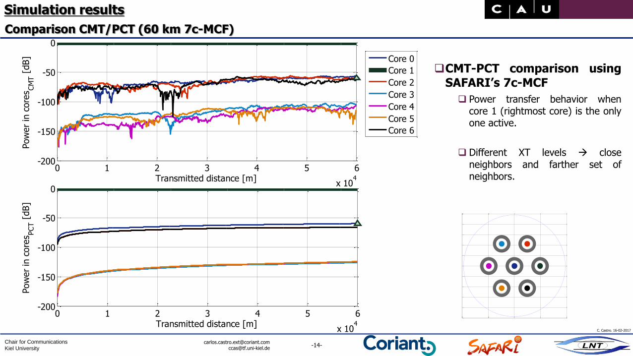
Simulation results

Comparison CMT/PCT (60 km 7c-MCF)

CMT-PCT comparison usingSAFARI’s 7c-MCF

Power transfer behavior whencore 1 (rightmost core) is the onlyone active.

Different XT levels close

neighbors and farther set ofneighbors.

0 1 2 3 4 5 6

x 104

-200

-150

-100

-50

0


Pow

er

in c

ore

s CM

T [

dB]

Core 0

Core 1

Core 2

Core 3

Core 4

Core 5

Core 6

0 1 2 3 4 5 6

x 104

-200

-150

-100

-50

0


Pow

er

in c

ore

s PCT [

dB]


Kiel University

C. Castro. 16-02-2017


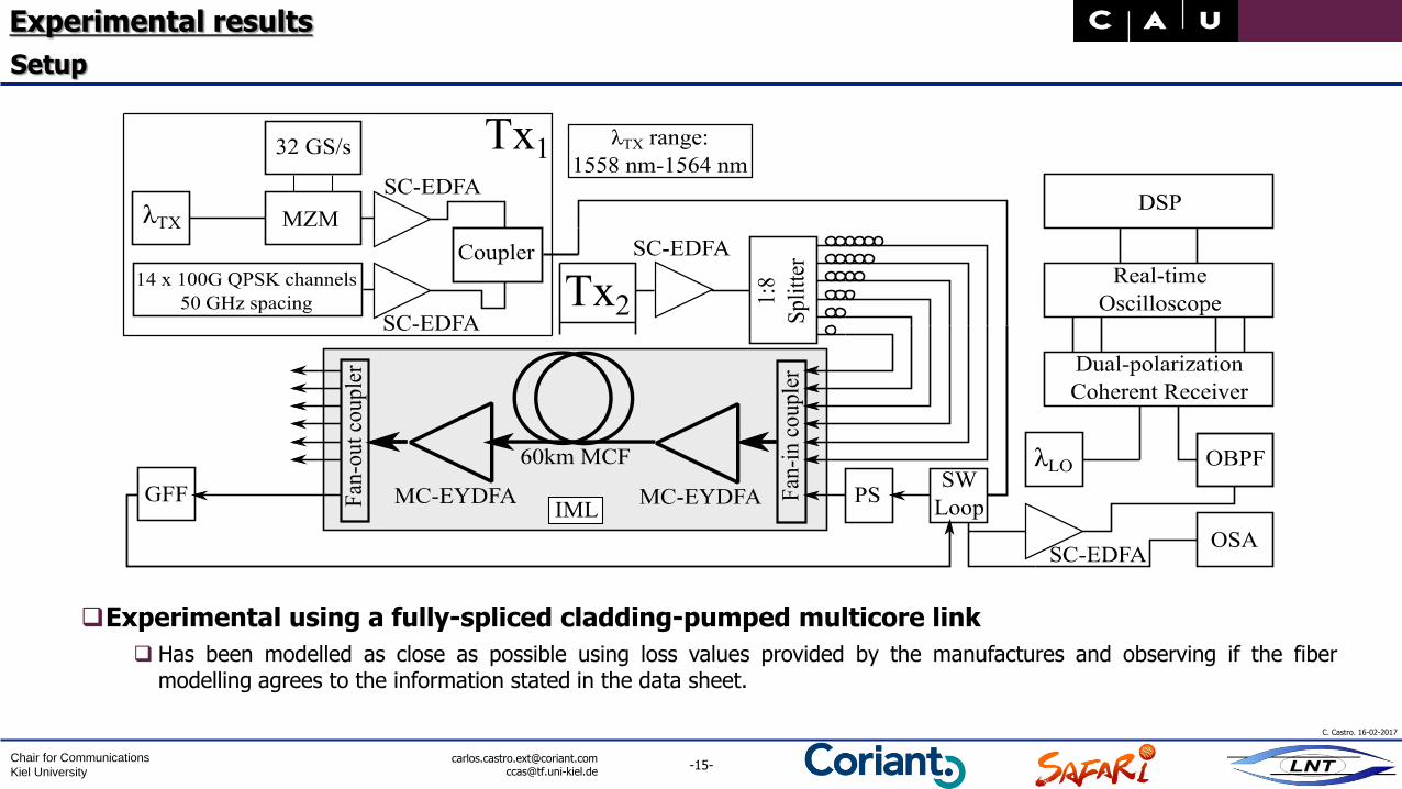
Experimental results

Setup

Experimental using a fully-spliced cladding-pumped multicore link

Has been modelled as close as possible using loss values provided by the manufactures and observing if the fibermodelling agrees to the information stated in the data sheet.


Kiel University

C. Castro. 16-02-2017


Experimental results

BER-Distance measurements

MCF System simulation(linear regime)

Measurementscorresponding to core 0.

AVG BER from 15 WDMchannels w/ channelspacing of 50 GHz

Only consideringimpairments mentioned inSlide 4.

Conclusion: simulationcan be used to roughlymodel a MCF system inorder to set transmissionobjectives accordingly.0 500 1000 1500 2000 2500 3000

10-5

10-4

10-3

10-2

10-1

100

Distance [km]

BER

FEC20%

3.4E-2

4QAMEXP

4QAMCMT

4QAMPCT

8QAMEXP

8QAMCMT

8QAMPCT

16QAMEXP

16QAMCMT

16QAMPCT


Kiel University

C. Castro. 16-02-2017



Summary and acknowledgements

Implementation of a FEM+CMT/PCT multicore fiber model

MCF system analysis for arbitrary MCF (structural and geometrical characteristics of the fiber)

FEM: calculation of cross-sectional field distribution and propagation constants of the individual cores

CMT/PCT are used to estimate the amount of XT after a given length MCF coupling matrix: digitally

simulate XT

Simulation results have been theoretically analyzed

MCF simulation has been compared to own experimental results using a fully-spliced cladding-pumpedmulticore fiber link (SAFARI project)

Coriant R&D, SAFARI project members, and Christian-Albrechts Universität zuKiel.

Chair for Communications

Kiel University

Thank you for your attention.

Workshop ITG-Fachgruppe 5.3.1 Simulation and … · Multicore fiber: a fiber-cladding structure...

Documents

Transcript of Workshop ITG-Fachgruppe 5.3.1 Simulation and … · Multicore fiber: a fiber-cladding structure...