What happened after the U.S. Bicentennial Celebration in 1976?
5757 S. University Ave.
Chicago, IL 60637
Main: 773.702.5599
bfi.uchicago.edu
WORKING PAPER · NO. 2019-56
What Happened to U.S. Business Dynamism? Ufuk Akcigit and Sina T. AtesAPRIL 2019
What Happened to U.S. Business Dynamism?∗†
Ufuk AkcigitUniversity of Chicago, NBER, CEPR
Sina T. AtesFederal Reserve Board
April 9, 2019
Abstract
In the past several decades, the U.S. economy has witnessed a number of striking trendsthat indicate a rising market concentration and a slowdown in business dynamism. In thispaper, we make an attempt to understand potential common forces behind these empiricalregularities through the lens of a micro-founded general equilibrium model of endogenousfirm dynamics. Importantly, the theoretical model captures the strategic behavior betweencompeting firms, its effect on their innovation decisions, and the resulting “best versus therest” dynamics. We focus on multiple potential mechanisms that can potentially drive theobserved changes and use the calibrated model to assess the relative importance of thesechannels with particular attention to the implied transitional dynamics. Our results highlightthe dominant role of a decline in the intensity of knowledge diffusion from the frontier firmsto the laggard ones in explaining the observed shifts. We conclude by presenting new ev-idence that corroborates a declining knowledge diffusion in the economy. We document ahigher concentration of patenting in the hands of firms with the largest stock and a changingnature of patents, especially in the post-2000 period, which suggests a heavy use of intellec-tual property protection by market leaders to limit the diffusion of knowledge. These findingspresent a potential avenue for future research on the drivers of declining knowledge diffusion.
Keywords: Business dynamism, market concentration, competition, knowledge diffusion,step-by-step innovations, transitional dynamics
JEL Classifications: E22, E25, L12, O31, O33, O34
∗First and foremost, we thank Richard Rogerson and John Haltiwanger for encouraging us to explore the declinein business dynamism in the United States. In addition, we thank Chiara Criscuolo, Chad Syverson, seminar andconference participants at the 7th CompNet Annual Conference, Boston College, Collège de France, the University ofTexas at Austin, the Federal Reserve Bank of Dallas, the OECD, the Central Bank of Turkey, the Bank of Italy, andthe Koc University Winter Workshop in Economics. Aakaash Rao and Zhiyu Fu have provided excellent researchassistance. Akcigit gratefully acknowledges financial support from the National Science Foundation. The views inthis paper are solely the responsibilities of the authors and should not be interpreted as reflecting the view of theBoard of Governors of the Federal Reserve System or of any other person associated with the Federal Reserve System.†E-mail addresses: [email protected], [email protected]
What Happened to U.S. Business Dynamism?
1 Introduction
Market economies are characterized by the so-called “creative destruction” where unproductiveincumbents are pushed out of the market by new entrants or other more productive incum-bents or both. A byproduct of this up-or-out process is the creation of higher-paying jobs andreallocation of workers from less to more productive firms. The U.S. economy has been losingthis business dynamism since the 1980s and, even more strikingly, since the 2000s. This shiftmanifests itself in a number of empirical regularities: The entry rate of new businesses, thejob reallocation rate, and the labor share have all been decreasing, yet the profit share, marketconcentration, and markups have all been rising. A growing literature has documented manydramatic empirical trends such as these and initiated a heated debate around the possible rea-sons behind the declining dynamism in the U.S. economy. We contribute to this important, andpredominantly empirical, debate by offering a new micro-founded macro model, conducting aquantitative investigation of alternative mechanisms that could have led to these dynamics, andpresenting some new facts on the rise of patenting concentration.
A central concern of our study is the identification of factors that could have driven theseobserved trends in U.S. business dynamism.1 During the past 30 years, the U.S. economy hasexperienced many fundamental changes that might have contributed to these trends shiftingthe power balance among competing firms toward market leaders. Some of these changes inprimitives, which we review in more detail in Appendix A, include reduced effective corporatetaxes, increased research and development (R&D) subsidies, increased regulations, and heavieruse of intellectual property, which limits the technologies that can be used by competing firmsand lowers the effective knowledge diffusion. Incorporating these margins within a realistictheoretical framework, we explore two main quantitative questions based on various thoughtexperiments in this study: First, how are the empirical trends observed since the 1980s linkedtogether? Second, could these trends be driven by changes discussed in this paragraph thatshifted the balance of market power?
Our research approach starts by summarizing the observed trends in the data and variouschanges in the economy that might have led to these trends. This initial discussion directs ourattention to a certain class of models. Accordingly, we build a theoretical model that accountsfor, in particular, endogenous market power and strategic competition among incumbents andentrants. Next, we calibrate this model to the U.S. economy as if it was in a steady state in1980 and hit the economy with four alternative shocks to make it enter into alternative transitionpaths. We then compare the model-generated paths with the actual trends to identify the mostpowerful shock in explaining all of the observed facts simultaneously. Finally, we calibrate the
1We focus on 10 specific trends: (i) market concentration has risen, (ii) average markups have increased, (iii) theprofit share of GDP has increased, (iv) he labor share of output has gone down, (v) the rise in market concentrationand the fall in labor share are positively associated, (vi) productivity dispersion of firms has risen, (vii) firm entry ratehas declined, (viii) the share of young firms in economic activity has declined, (ix) job reallocation has slowed down,and (x) the dispersion of firm growth has decreased. We review them in more detail in Section 2.
1
What Happened to U.S. Business Dynamism?
transition path of the model economy to reflect the changes that the U.S. economy has beenexperiencing in the past several decades. We then decompose the contribution of each channel ofinterest to the model-generated trends in order to quantify their potential importance in drivingthe empirical regularities that the U.S. economy has been witnessing.
A key advantage of studying 10 empirical trends jointly (as opposed to a smaller subset ofthem) with the help of a general equilibrium model is to exploit the power of “overidentification.”A single empirical fact can potentially be explained by multiple alternative mechanisms; however,multiple empirical facts can (we hope) help us identify one single mechanism that might haveled to the observed trends in the United States.
In a recent piece, Syverson (2019) emphasizes that the topic of “market power” has histori-cally been studied mostly by micro industrial organization literature, which focused its attentionon specific industries. While he welcomes the paradigm shift in macroeconomics toward thistopic and its aggregate implications, he explains in detail why the macroeconomic discussionshould rely more on microeconomic foundations. In this regard, our goal is to pull the macroand micro literatures closer by building a macro general equilibrium model that draws heavily onan early industrial organization literature that investigated the competition dynamics among in-cumbent firms in a winner-take-all race (e.g., Harris and Vickers, 1985, 1987; Budd et al., 1993). Inthe typical framework, two players race for a prize, and players exert different efforts dependingon their own position relative to their competitors. A fruitful branch of endogenous growth liter-ature has introduced these partial equilibrium models into a macro general equilibrium setting inorder to study various aspects of product market competition with strategic interaction betweencompeting firms (e.g., Aghion et al., 1997, 2001, 2005; Acemoglu and Akcigit, 2012; Akcigit etal., 2018). In a recent review of declining business dynamism, we consider a framework alongthese lines (Akcigit and Ates, 2019). The study presents a first-step discussion of the theoreticalpredictions of the standard model in comparison with the empirical evidence. In this paper, weextend the standard framework to have a richer setting suitable for quantitative analysis.
Similar to these studies, our theoretical framework centers on an economy that consists ofmany sectors. In each sector, two incumbent firms, which can also be interpreted as the best andthe rest, compete à la Bertrand for market leadership. This competitive structure forces marketleaders to post a limit price; hence, the mark-ups evolve endogenously as a function of thetechnology gap between firms. Market leaders try to innovate in order to open up the lead andincrease their markups and profits. Follower firms try to innovate with the hope of eventuallyleapfrogging the market leader and gaining market power. Likewise, new firms attempt to enterthe economy with the hope of becoming a market leader some day. A very important aspect ofthe model is the strategic innovation investment by the firms: Intense competition among firms,especially when the competitors are in a neck-and-neck position in terms of their productivitylevels, induces more aggressive innovation investment and more business dynamism. Yet whenthe leaders open up their technological lead, followers lose their hope of leapfrogging the leader
2
What Happened to U.S. Business Dynamism?
and lower their innovation effort. Likewise, entrants get discouraged when the markets areoverwhelmingly dominated by the market leader, and the entry rate decreases.
Our structural model allows us to primarily analyze four important margins that shapethe competition dynamics. First, corporate taxes affect profits and the return to being the mar-ket leader. Second, the government supports incumbents’ productivity-enhancing investmentsthrough R&D subsidies. Third, the level of entry costs affect the incentives of potential new en-trants. Finally, the amount of knowledge diffusion in the economy allows followers to copy themarket leaders and remain close to them. Incidentally, the U.S. economy has observed significantchanges along all of these margins in the past several decades. Changes in these four marginshave different implications as to how competition and business dynamism evolve over time inour model. Thus, our model allows us to run a horse race between these important channelsand ascertain which one(s) among them has greater power in explaining the observed empiricaltrends in the U.S. economy.
We calibrate the model to pre-1980 moments in the data as if the U.S. economy was in asteady state. We then conduct two sets of experiments. The first set of experiments focuses oneach of the four channels individually, illustrating the potential of each channel in generating ob-served empirical trends. For instance, we implement a large drop in the effective corporate taxrates between 1980 and 2010 and compare the model-simulated transition paths with all post-1980 empirical trends. We repeat this analysis with all four channels described previously. Thesecond set of experiments matches the transition path of the model to the transitional dynamicsof the U.S. economy, allowing all four channels to move jointly, and then quantifies their indi-vidual contributions. Both sets of exercises indicate that, even though each channel can havesome effect at different levels, reduction in knowledge diffusion between 1980 and 2010 is the mostpowerful force in driving all of the observed trends simultaneously. For instance, while each ofthe remaining channels can rarely account for more than 10 percent of the observed trends, theknowledge diffusion channel accounts for more than 70 percent of most symptoms of decliningbusiness dynamism and at least 50 percent of all considered trends.
Reduction in knowledge diffusion is able to account for these trends as follows. When knowl-edge diffusion slows down over time, as a direct effect, market leaders are shielded from beingcopied, which helps them establish stronger market power. When market leaders have a biggerlead over their rivals, the followers get discouraged; hence, they slow down. The productivitygap between leaders and followers opens up. The first implication of this widening is that marketcomposition shifts to more concentrated sectors. Second, limit pricing allows stronger leaders(leaders further ahead) to charge higher markups, which also increases the profit share and de-creases the labor share of gross domestic product (GDP). Since entrants are forward looking,they observe the strengthening of incumbents and get discouraged; therefore, entry goes down.Discouraged followers and entrants lower the competitive pressure on the market leader: Whenthey face less threat, market leaders relax and they experiment less. Hence, overall dynamism
3
What Happened to U.S. Business Dynamism?
and experimentation decrease in the economy.
Although the main goal of this paper is positive rather than normative, we also discussbriefly the welfare implications of market concentration within the framework of our model. Aninteresting observation is that lower market concentration is not always welfare enhancing. Incases when the knowledge diffusion is high and competition is too fierce, weighing on leaderfirms’ innovation incentives, a lower level of knowledge diffusion can improve aggregate inno-vation and welfare. However, our quantitative results indicate that in the calibrated baselineeconomy, a higher rate of knowledge diffusion is unequivocally welfare improving, implyingthat the baseline diffusion rate is inadequate from a welfare perspective.
We conclude our quantitative analysis with various robustness exercises and discuss somemodel extensions. We also elaborate on three additional channels—a decline in the inter-est rate, a fall in research productivity, and a decrease in workers’ market power relative toemployers/firms—whose potential links to some of the observed trends considered here haverecently drawn the attention of the literature. We assess the potential of these channels in jointlyaccounting for the empirical trends under consideration and show that each one of them leadsto some counterfactual response in a number of margins.
As a cautious remark, our results do not mean, and are far from implying, that the declinein knowledge diffusion is the only driver of the observed trends. Indeed, each empirical trendmight have its own leading factors, and those factors may be different than the ones studiedhere. However, our analysis instead shows that among the mechanisms we consider—changesin corporate taxation, government support for incumbents, increased regulatory burden, andreduced knowledge diffusion (potentially due to anticompetitive use of intellectual property)—the last one stands out as a powerful force when 10 empirical facts are considered together.Therefore, our results stress the importance of future research to understand the underlyingreasons for slower knowledge diffusion. To this end, we conclude our study by presentingsome brand-new, striking trends on the increased concentration of patents through both theirproduction and purchase by market leaders, as well as on the strategic use of patents, especiallysince the early 2000s. We hope that these findings ignite a broader conversation in the literature.
The rest of the paper is organized as follows. Section 2 reviews the literature; it also re-visits the empirical trends that the literature has interpreted as the signs of declining businessdynamism. After presenting the empirical evidence that motivates the theory, Section 3 intro-duces the theoretical model, and Section 4 describes its calibration. Sections 5 and 6 presentthe experiments that identify and quantify the importance of each margin using the calibratedmodel. Section 7 discusses the welfare implications. Section 8 presents robustness exercises,discusses model extensions, and investigates the implications of additional channels with regardto observed empirical trends. Section 9 provides some new empirical facts on the distribution ofthe use of intellectual property in the U.S. economy, which could shed some light on the reasonwhy knowledge diffusion has slowed down over time. Section 10 concludes.
4

What Happened to U.S. Business Dynamism?
2 Empirical Regularities and Literature Review
While the contribution of our work is mainly quantitative, it draws heavily on empirical workin the literature. Therefore, in this section, we first review the findings of this literature. Tosummarize, we focus on the following empirical regularities:
1. Market concentration has risen.
2. Average markups have increased.
3. The profit share of GDP has increased.
4. The labor share of output has gone down.
5. The rise in market concentration and the fall in labor share are positively associated.
6. Productivity dispersion of firms has risen. Similarly, the labor productivity gap betweenfrontier and laggard firms has widened.
7. Firm entry rate has declined.
8. The share of young firms in economic activity has declined.
9. Job reallocation has slowed down.
10. The dispersion of firm growth has decreased.
Next, we will briefly discuss the mechanisms the literature has proposed to explain these regu-larities. We refer the interested reader to Akcigit and Ates (2019) for a more extensive review.
To start, a set of recent papers document an increasing market concentration in the UnitedStates (Fact 1; see Furman and Giuliano, 2016; Autor et al., 2017a,b; Barkai, 2017; Grullon et al.,2017; and Gutiérrez and Philippon, 2016, 2017, among others).2 Second, several recent studiesshow an increase in average markups (Fact 2; see Nekarda and Ramey, 2013; De Loecker andEeckhout, 2017; Gutiérrez and Philippon, 2017; Eggertsson et al., 2018; and Hall, 2018, amongothers).3 Relatedly, a subset of these studies also highlight an increase in the aggregate profitshare (Fact 3). These findings drew considerable attention from both academic and policy circles,as they likely indicate an increase in firms’ market power and a decline in industry competition.For instance, Gutiérrez and Philippon (2016) argue that increased industry concentration drivesthe weak investment performance of U.S. firms via a decline in competition. Eggertsson et al.(2018) and Farhi and Gourio (2018) argue that increased market power can help explain severalmacro-finance regularities, with Eggertsson et al. (2018) also emphasizing persistently low inter-est rates. Liu et al. (2019) also focus on the role of low interest rates as a culprit of rising marketconcentration and declining business dynamism.4 Barkai (2017) claims that higher concentration
2Bajgar et al. (2019) and Kalemli-Ozcan et al. (2019) document similar patterns for European countries as well,focusing on consolidated firm accounts.
3Calligaris et al. (2018) and De Loecker and Eeckhout (2018) document similar patterns for various other countriesas well.
4We discuss the effects of declining interest rates further in Section 8.1.
5
What Happened to U.S. Business Dynamism?
is associated with lower competition and results in a declining factor income of labor. However, itis worth noting that higher market concentration may not necessarily imply higher market powerof firms (Syverson, 2004a,b). In fact, Autor et al. (2017b) and Bessen (2017) contend that highermarket concentration is a result of higher market competition and the rise of more productivefirms.5 Bessen (2017) documents that sales concentration is strongly correlated with the use ofinformation and communication technologies at the industry level. In a similar vein, Crouzetand Eberly (2018) observe that at the industry level, the firms with the largest size and highestgrowth rate are the ones whose investment in intangible capital grows the fastest.6
The fourth regularity that we include in our analysis is the secular decline in the aggregatelabor share of GDP in the United States (Fact 4; see Karabarbounis and Neiman, 2013; Elsby et al.,2013; and Lawrence, 2015). The literature has proposed a variety of explanations for this decline,including increased offshoring or foreign sourcing of inputs (Elsby et al., 2013, and Boehm etal., 2017); a fall in corporate tax rates (Kaymak and Schott, 2018); a slowdown in populationgrowth (Hopenhayn et al., 2018); a slowdown in productivity growth (Grossman et al., 2017);higher prevalence of robots in production and replacement of production workers by automatedmachinery (Acemoglu and Restrepo, 2017); and declining competition due to increased marketconcentration (Barkai, 2017). Autor et al. (2017b) also consider higher market concentration asa driver of declining labor share but relate it to the emergence of winner-take-all dynamics inmany industries with a rise of “superstar” firms.7 They highlight the positive industry–levelrelationship between the rise in concentration and the fall of labor share, another regularitywe consider in this paper (Fact 5). In a recent study, Aghion et al. (2019) also focus on thisrelationship in an endogenous growth model à la Klette and Kortum (2004), extending the modelto zero in on the relocation of activity between incumbent firms (abstracting from firm entry)across balanced growth paths.8
We also consider some facts that suggest a decline in business dynamism. First, the produc-tivity dispersion has increased in the United States, as shown by Decker et al. (2018). Similarly,Andrews et al. (2015, 2016) establish that, across the OECD economies, the gap between the av-erage productivity levels of frontier firms (top 5 percent of firms with the highest productivity)and the laggard ones has been widening, suggesting the rise of “best versus the rest” dynamics,a relationship captured by the market structure of our theoretical model (Fact 6). Second, there
5While most of these papers analyze industries at the national level, Rossi-Hansberg et al. (2018) find that, forseveral industries, the increase in market concentration at the national level coincides with a decline in concentrationat the local level, raising the question of the “relevant” market. Some policymakers bring forward similar critiquesbased on the definition of relevant markets (see OECD, 2018b, by the U.S. delegation and OECD, 2018a).
6Gutiérrez and Philippon (2019) also note that the two explanations—rising market power and decreasing com-petition versus the rise of more efficient “superstar” firms—do not necessarily describe mutually exclusive stories inthat leaders can become more efficient while using this advantage to also become “more entrenched.”
7 Diez et al. (2018) also find support for the superstar-firm argument in an international comparison using multi-country firm-level data. However, recent work by Gutiérrez and Philippon (2019) argues that the superstar firms havebeen losing their share in economic activity in the United States, especially in the post-2000 period.
8Using a similar setting, De Ridder (2019) shows that the effect of an increase in firms’ efficiency of technologyadoption can depress aggregate innovation in a balanced growth path while increasing market power of firms.
6
What Happened to U.S. Business Dynamism?
has been a secular decline in firm (and establishment) entry rates in the United States in the pastseveral decades (Fact 7; see Decker et al., 2016b; Gourio et al., 2014; and Karahan et al., 2016).Likewise, the employment share of young firms has also been declining steadily (Fact 8; seeDecker et al., 2016b, and Furman and Orszag, 2018), which is particularly worrying given the dis-proportionate contribution of high-growth young firms to job creation (Bravo-Biosca et al., 2013,and Haltiwanger et al., 2013). Decker et al. (2016a) also provide two additional regularities—namely, the decline in the gross job reallocation rate (Fact 9) and the fall in the dispersion of firmgrowth rates (Fact 10). The authors claim that these observations are driven by the shrinkingcontribution of high-growth young firms to economic activity, which in turn they attribute to thedeclining responsiveness of firms to idiosyncratic productivity shocks. Pugsley et al. (2018) ar-gue that the fall in rapid-growth young firms (gazelles) is due to a structural shift in the ex-anteheterogeneity of firms in the United States, with a decline in the prevalence of high-potentialfirms. Emphasizing the effects of the Great Recession, Davis and Haltiwanger (2019) highlightthe role of housing market cycles and credit conditions in the decline of young firm activity.
Our investigation finds that a decline in knowledge diffusion explains the large set of trendsin the data. The widening productivity gap between frontier and laggard firms, as illustrated byAndrews et al. (2016), may be indicative of a distortion in the flow of knowledge between thesefirms. The authors stress that digitalization and the increasing reliance of production processeson tacit knowledge may disproportionately benefit frontier firms in ways that cannot be easilyincorporated by laggard firms. Thus, the changing nature of technologies and the increasingimportance of tacit knowledge in the form of big and proprietary data could limit spillovers fromfrontier to laggard firms. For instance, data-dependent production processes could generate data-network effects—more data helps an incumbent firm serve customers better, thus attracting morecustomers, which in turn generates more data that improve services, which in turn entices morecustomers—that put large and established firms that produce large databases in an advantageousposition (The Economist, 2017). Indeed, Calligaris et al. (2018) find that markup differencesbetween frontier and laggard firms are the highest in digitally-intensive sectors. These dynamicsresonate also with the findings of Grullon et al. (2017) that U.S. firms in the most concentratedindustries hold the largest and relatively more valuable patent portfolios.
Regulations are another factor that could hamper technology diffusion between frontier andlaggard firms. In this regard, anticompetitive effects of weak antitrust laws and enforcement havebeen raised as a concern (Grullon et al., 2017). Indeed, a strand in the law literature emphasizesthe paradigm shift in the application of antitrust laws in a direction that underlines productmarket efficiency rather than size-based concentration in the interpretation of laws (Baker, 2012;Khan, 2016; Lynn, 2010). Lower antitrust enforcement and increased consolidation could harmthe competitive dynamics of the market. For instance, Cunningham et al. (2018) underscore the“killer acquisitions” in the pharmaceutical industry, preemptive mergers to buy out a potentialfuture competitor. Such consolidation may cause large firms to focus on defending their stakesrather than investing in productive activity, limiting the potential flow of knowledge to follower
7
What Happened to U.S. Business Dynamism?
firms and its productive use by them. Bessen (2016) observes that rent-seeking and lobbyingactivity have gained traction in the United States in the post-2000 period. These argumentsresonate with the findings of Andrews et al. (2016), who claim that the lack of pro-competitiveproduct market reforms has contributed to the widening productivity gap between frontier andlaggard firms across the OECD countries.
To sum up briefly, our study takes a holistic approach to account for all of the empiricaltrends mentioned in this section. We analyze shifts in market power and business dynamicsjointly as endogenous market outcomes through the lens of a structural model instead of takingthem as “market primitives” as criticized by Syverson (2019). Moreover, our quantitative analy-sis, carefully accounting for transitional dynamics, evaluates the strength of potential channelsthat could have contributed to the observed changes and underscores the dominant role playedby the knowledge diffusion margin. Finally, we advance the debate on market concentrationand business dynamism by presenting new evidence from patent data that highlights changingconcentration patterns.
3 Model
This section presents a closed-economy endogenous growth model of strategic interaction andinnovation in which firms compete over the ownership of intermediate-good production. Theeconomy is composed of a continuum of intermediate goods that are inputs in the productionof the final good, which is in turn consumed by the representative households. In each interme-diate product line, two active incumbent firms engage in Bertrand price competition to obtain amonopoly of production. Intermediate firms produce using labor and are heterogeneous in theirproductivity and thus in the marginal cost of production. Firms invest in cost-saving innovativeactivity to improve their productivity in the spirit of step-by-step models, which allows for het-erogeneous technological gaps between competitors. An appealing feature of the model is that,combined with optimal limit pricing that stems from Bertrand competition, different relative pro-ductivity levels generate a distribution over heterogeneous markup levels. In addition, there isan outside pool of entrants that engage in research activity to enter the market by replacing thetechnological follower in a particular line.
Among several channels that affect firm incentives in our model, we include a probability ofexogenous technology spillovers that, once realized, allow a technological laggard firm to closethe gap with the frontier. This channel governs the knowledge diffusion between the techno-logical frontier and the follower, one of the main channels that we consider in our quantitativeinvestigation as potential drivers of the declining business dynamism in the United States. In themodel, the implications of these potential factors hinge on their effect on the distribution of firmsacross relative technology levels and the resulting transitional dynamics, whose law of motionswe describe in this section.
8
What Happened to U.S. Business Dynamism?
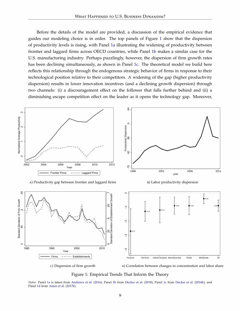
Before the details of the model are provided, a discussion of the empirical evidence thatguides our modeling choice is in order. The top panels of Figure 1 show that the dispersionof productivity levels is rising, with Panel 1a illustrating the widening of productivity betweenfrontier and laggard firms across OECD countries, while Panel 1b makes a similar case for theU.S. manufacturing industry. Perhaps puzzlingly, however, the dispersion of firm growth rateshas been declining simultaneously, as shown in Panel 1c. The theoretical model we build herereflects this relationship through the endogenous strategic behavior of firms in response to theirtechnological position relative to their competitors. A widening of the gap (higher productivitydispersion) results in lower innovation incentives (and a declining growth dispersion) throughtwo channels: (i) a discouragement effect on the follower that falls further behind and (ii) adiminishing escape competition effect on the leader as it opens the technology gap. Moreover,
0.1
.2.3
Nor
mal
ized
Ave
rage
Pro
duct
ivity
2002 2004 2006 2008 2010 2012Year
Frontier Firms Laggard Firms
a) Productivity gap between frontier and laggard firms
.78
.82
.86
.9.9
4Pr
oduc
tivity
Dis
pers
ion
1996 2001 2006 2011year
b) Labor productivity dispersion
.5.5
5.6
.65
.7St
anda
rd D
evia
tion
of E
stab
lishm
ent G
row
th
.4.4
5.5
.55
Stan
dard
Dev
iatio
n of
Firm
Gro
wth
1980 1990 2000 2010Year
Firms Establishments
c) Dispersion of firm growth
−0.27
−0.13−0.12
−0.09 −0.09 −0.09
−0.04
−.4−.3
−.2−.1
0
Finance Services Utils&Transport Manufacturing Retail Wholesale All
d) Correlation between changes in concentration and labor share
Figure 1: Empirical Trends That Inform the Theory
Notes: Panel 1a is taken from Andrews et al. (2016), Panel 1b from Decker et al. (2018), Panel 1c from Decker et al. (2016b), andPanel 1d from Autor et al. (2017b).
9
What Happened to U.S. Business Dynamism?
Panel 1d suggests a negative correlation between concentration and labor share at the industrylevel. Our theoretical model reflects this relationship through the shift of production to moreproductive frontier firms as the technology gap between them and the laggards opens up. Insum, the endogenous competition structure of our framework helps us speak to salient featuresof changing business dynamism in the United States. Now we present the model details.
3.1 Preferences
We consider the following continuous-time economy. In this environment, there is a representa-tive consumer that derives logarithmic utility from consumption:
Ut =∫ ∞
texp (−ρ (s− t)) ln Cs ds,
where Ct represents consumption at time t and ρ > 0 is the discount rate. The budget constraintof the representative consumer reads as
Ct + At = wtLt + rt At + Gt,
where Lt denotes labor (supplied inelastically), At denotes total assets, and Gt denotes lump-sum taxes levied or transfers distributed by the government. We normalize labor supply suchthat Lt = 1. The relevant prices are the interest rate rt, the wage rate wt, and the price of theconsumption good Pt, which we take to be the numeraire. Because households own the firms inthe economy, the asset market clearing condition implies that the total assets At equal the sumof firm values, i.e., At =
∫F Vf t d f with F denoting the measure of firms.
3.2 Technology and Market Structure
3.2.1 Final Good
The final good, which is used for consumption, is produced in perfectly competitive marketsaccording to the following production technology:
ln Yt =∫ 1
0ln yjt dj, (1)
where yjt denotes the amount of intermediate variety j ∈ [0, 1] used at time t. Each variety isproduced by a monopolist, which we describe next.
10
What Happened to U.S. Business Dynamism?
3.2.2 Intermediate Goods and Innovation
Incumbents. In each product line j, two incumbent firms i = {1, 2} produce two perfectlysubstitutable varieties of intermediate good j according to a linear production technology:
yijt = qijtlijt,
where lijt denotes the labor employed and qijt is the associated labor productivity of firm i. Thetotal industry output is given by yjt = yijt + y−ijt, where −i denotes the competitor of firm iwith −i = {1, 2} and −i 6= i. The intermediate-good firms compete for market leadership àla Bertrand. As a result, the firm that has a higher labor productivity obtains a cost advantageand therefore captures the whole market to supply the intermediate good j. We call a firm i themarket leader (follower) in j if qij > q−ij (qij < q−ij). Firms are neck-and-neck if qij = q−ij. Wenormalize initial productivity levels to unity such that qij0 = 1.
Firms’ productivity evolves through successive innovations. When a leader innovates be-tween t and t + ∆t, its productivity level improves proportionally by a factor λ > 1 such thatqij(t+∆t) = λqijt. By contrast, an innovation by a follower may be an incremental or drastic one.With probability (1− φ), the follower’s innovation improves its productivity proportionally byλ, as in the case of leader innovation—a process called slow catch-up (see Acemoglu and Akcigit,2012). With probability φ, a follower can incidentally come up with an innovation that bringsabout a drastic improvement in productivity, allowing the follower to close the gap with theleader—a process called quick catch-up.
Another source of quick catch-up is the flow of knowledge between competitors. In par-ticular, we assume that quick catch-up can also occur at an exogenous Poisson flow rate δ. Inthis case, the follower can replicate the frontier technology and catch up with the leader. In asense, this exogenous catch-up probability reflects the degree to which followers can learn fromthe technology frontier, capturing, in essence, spillovers from the “best” to “rest” of the firms.Therefore, we label δ as the “knowledge diffusion” parameter.
In each product line, the leader and the follower are separated by a certain number of tech-nology gaps, which reflect the difference between the total number of technology rungs thesefirms’ productivities build on. Specifically, suppose that, in line j, firm i’s productivity levelreflects nijt past improvements. Then the relative productivity level is given by
qijt
q−ijt=
λnijt
λn−ijt= λnijt−n−ijt ≡ λmijt ,
where mijt ∈N defines the technology gap between firm i and the competitor−i. We assume thatthere is a large but exogenously given upper limit in the technology gap, denoted by m.9 As will
9This innocuous assumption renders the state space finite and enables the computation of the equilibrium.
11

What Happened to U.S. Business Dynamism?
be clear, mijt is a sufficient statistic to describe firm-specific payoffs independent of the productline j. Therefore, we will drop industry subscript j whenever mit ∈ {−m, ..., 0, ..., m} refers to afirm-specific value. Accordingly, when we say the leader is m-steps ahead or, reciprocally, thefollower is m-steps behind, we mean that the follower needs to improve its productivity m stepsmore than the leader to become neck-and-neck. Lastly, we will use the notation mjt ∈ {0, ..., m}to denote the technology gap between competitors in sector j. We call sectors with positive gaps(mjt > 0) “unleveled” and sectors with no gap (mjt = 0) neck-and-neck or “leveled.”
Firms invest in R&D to obtain or retain market leadership by improving their productivity.To conduct R&D, firms hire labor. When a firm employs hijt R&D workers, it generates aninnovation with the arrival rate of xijt. Let Rijt denote the R&D expenditures of firm i in productline j at time t. We consider a convex cost of generating the arrival rate xijt in the form of
Rijt = αxγ
ijt
γwt,
where γ is the (inverse) elasticity of R&D with respect to R&D workers and wt denotes thewage rate that prevails in the economy. As a result, the R&D production function is given by
xijt =(
γhijtα
) 1γ.
Entrants. Every period, a new entrepreneur in each product line invests in R&D to enter thebusiness. If the entrepreneur generates a successful innovation, it replaces the follower in theproduct line (or one of the two incumbents with the same probability if it enters a neck-and-neckline).10 If the innovation attempt fails, the entrant disappears.
Similar to the follower innovation, an entrant innovation may be drastic, with probability φ,allowing it to catch up with the frontier technology.11 With probability (1− φ), the innovationis incremental, improving on the productivity level of the existing follower proportionally withstep size λ. If the entrant hires hijt R&D workers, it generates an innovation arrival rate xijt, andthe expenditures on R&D investment are given by
Rijt = αxγ
ijt
γwt.
We assume that firms benefit from knowledge diffusion only after they enter the market andengage in perpetual innovative activity. This distinction between entrant and follower firms willhighlight the role of distortions to the knowledge flow between frontier and laggard firms indriving business dynamism and, in particular, firm entry, even when no direct negative effect on
10The process of entrants replacing the follower or neck-and-neck firms reflects the data where entrants enter themarket small and never as large conglomerates.
11 In the remainder of the discussion, a “ ˜ ” sign will refer to values that pertain to an entrant.
12
What Happened to U.S. Business Dynamism?
firm entry is assumed. As we shall see, this margin proves crucial in understanding empiricaltrends.
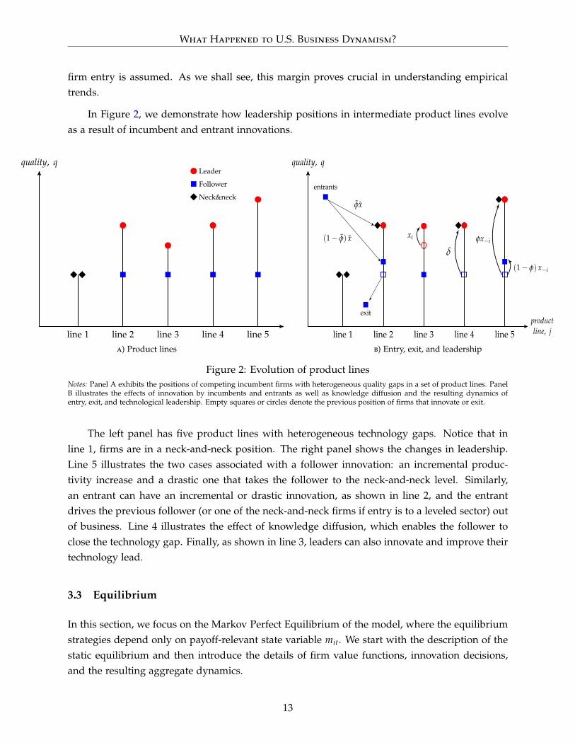
In Figure 2, we demonstrate how leadership positions in intermediate product lines evolveas a result of incumbent and entrant innovations.
quality, q
productline, j
Leader
Follower
Neck&neck
line 1 line 2 line 3 line 4 line 5
δ
(1− φ) x−i
φx−i
entrants
φx
(1− φ) x
exit
a) Product lines
quality, q
productline, jline 1 line 2 line 3 line 4 line 5
xi
δ
(1− φ) x−i
φx−i
entrants
φx
(1− φ) x
exit
b) Entry, exit, and leadership
Figure 2: Evolution of product linesNotes: Panel A exhibits the positions of competing incumbent firms with heterogeneous quality gaps in a set of product lines. PanelB illustrates the effects of innovation by incumbents and entrants as well as knowledge diffusion and the resulting dynamics ofentry, exit, and technological leadership. Empty squares or circles denote the previous position of firms that innovate or exit.
The left panel has five product lines with heterogeneous technology gaps. Notice that inline 1, firms are in a neck-and-neck position. The right panel shows the changes in leadership.Line 5 illustrates the two cases associated with a follower innovation: an incremental produc-tivity increase and a drastic one that takes the follower to the neck-and-neck level. Similarly,an entrant can have an incremental or drastic innovation, as shown in line 2, and the entrantdrives the previous follower (or one of the neck-and-neck firms if entry is to a leveled sector) outof business. Line 4 illustrates the effect of knowledge diffusion, which enables the follower toclose the technology gap. Finally, as shown in line 3, leaders can also innovate and improve theirtechnology lead.
3.3 Equilibrium
In this section, we focus on the Markov Perfect Equilibrium of the model, where the equilibriumstrategies depend only on payoff-relevant state variable mit. We start with the description of thestatic equilibrium and then introduce the details of firm value functions, innovation decisions,and the resulting aggregate dynamics.
13
What Happened to U.S. Business Dynamism?
Households. Optimal household decisions determine the equilibrium interest rate of the econ-omy. The Euler equation implies
rt = gt + ρ, (2)
where gt is the growth rate of output.
Final- and Intermediate- Good Production. The optimization of the representative final-goodproducer generates the following demand schedule for the intermediate good j ∈ [0, 1]:
yijt =Yt
pijt, (3)
where pijt is the price of intermediate good j that the monopolist producer i charges. The unit-elastic demand schedule implies that the final-good producer spends an equal amount Yt on eachintermediate good j.
Given the linear production function, an intermediate producer’s marginal cost becomes
mcit =wt
qit, (4)
which increases in the wage rate and decreases in the firm’s labor productivity.12 Moreover,Bertrand competition leads to limit pricing such that the intermediate producer sets its price tothe marginal cost of its competitor:
pit =wt
q−it. (5)
Then the optimal equilibrium quantities of the intermediate varieties produced are given as
yit =
q−itωt
if qit > q−it
0 if qit < q−it
, (6)
where ωt ≡ wt/Yt denotes the normalized wage level. We assume that in neck-and-neck sectors,i.e., when qit = q−it, the production is assigned randomly to both firms. The optimal productionemployment of the intermediate producer follows as
lit =yit
qit=
1ωtλmit
for mit ≥ 0. (7)
The operating profits of the intermediate producer exclusive of R&D expenditures becomes
π (mit) = (pit −mcit) yit =
(1− 1
λmit
)Yt for mit ≥ 0, (8)
12 We dropped the subscript j for brevity and will do so in the remainder fo the discussion unless it would causeconfusion.
14
What Happened to U.S. Business Dynamism?
and π (mit) = 0 otherwise. Similarly, the price–cost markup reads as
mk (mit) =pit
mcit− 1 = λmit − 1 for mit ≥ 0, (9)
and mk (mit) = 0 otherwise. Notice that markups, and thus profits, are positive only for marketleaders and depend on the technological difference between the leader and the follower. As such,this structure provides a useful ground to analyze the markup dynamics in the economy, whichare determined by the distribution of industries across heterogeneous gap differences, which inturn evolve based on firms’ endogenous innovation decisions.
3.3.1 Firm Values and Innovation
Incumbents. We denote the stock market value of an incumbent firm in the payoff-relevantstate mit at time t by Vmt (dropping the subscripts on m for simplicity). Then the value functionof a leader that is m-steps ahead is given by
rtVmt − Vmt = maxxmt
{(1− τt)
(1− 1
λm
)Yt − (1− st) α
xγmtγ
wt + xmt [Vm+1t −Vmt]
+ (φx−mt + φx−mt + δ) [V0t −Vmt]
+ ((1− φ) x−mt + (1− φ) x−mt) [Vm−1t −Vmt]} . (10)
The first line on the right-hand side of the expression captures the profits net of R&D expen-ditures, taxed at the corporate income tax rate τt. The second term in the first line is the ex-penditures on R&D, which is subsidized by the government at rate st. The last term capturesthe improvement in a leader’s position as a result of successful innovation.13 As reflected in thesecond line, if there is a drastic innovation by the follower or by an entrant, or if knowledgediffuses at rate δ, the leader finds itself in a neck-and-neck position. Finally, the last line of theexpression captures the case of nondrastic innovation by competitors, in which the position ofthe leader deteriorates by one step.
Similarly, the value of an m-step follower is defined as
rtV−mt − V−mt = maxx−mt
{− (1− st) α
xγ−mt
γwt + (1− φ) x−mt [V−m+1t −V−mt]
+ (φx−mt + δ) [V0t −V−mt]
+xmt [V−m−1t −V−mt] + x−mt [0−V−mt]} . (11)
Notice that the follower does not produce and, therefore, does not generate any profits. Nev-ertheless, forward-looking followers invest in R&D with the prospect of taking over the leader
13 When the m-step leader innovates, the gap does not increase because of the imposition of an upper limit on thepotential size of gaps. As a result, an m-step leader optimally chooses not to invest in R&D.
15
What Happened to U.S. Business Dynamism?
through successive innovations and reaping potential profits. Moreover, a drastic innovation andthe exogenous catch-up shock can bring them directly to the frontier. When there is successfulentry to the product line, the follower exits the market, receiving a continuation value of zero.Finally, the value of a neck-and-neck incumbent is given by14
rtV0t − V0t = maxx0t
{− (1− st) α
xγ0tγ
wt + x0t [V1t −V0t] + x0t [V−1t −V0t] +12
x0t [0−V0t]
}. (12)
Before we compute optimal innovation efforts, the next lemma defines the normalized firmvalues, which render the problem stationary.
Lemma 1 Define the normalized value vmt such that Vmt = vmtYt. Then, for m > 0, vmt is given by
ρvmt − vmt = maxxmt
{(1− τt)
(1− 1
λm
)Yt − (1− st) α
xγmtγ
wt + xmt [vm+1t − vmt]
+ (φx−mt + φx−mt + δ) [v0t − vmt]
+ ((1− φ) x−mt + (1− φ) x−mt) [vm−1t − vmt]} .
Normalized values for m ≤ 0 are defined reciprocally.
Proof. These normalized values follow directly from using the definition Vmt = vmtYt andsubstituting households’ Euler condition given in equation (2).
The first order conditions of the problems defined earlier yield the following optimal inno-vation decisions:
xmt =
[
1α(1−st)
(vm+1t − vmt)] 1
γ−1if m ≥ 0[
1α(1−st)
{(1− φ) vm+1t + φv0t − vmt}] 1
γ−1if m < 0
. (13)
Entrants. Recall that entry is directed at particular product lines, and a successful entrant re-places the follower (or one of the incumbents with an equal probability if entry is to a line in aneck-and-neck state). The problem of an entrant that aims for a product line with an m-step gapis given as
maxx−mt
{−α
xγ−mt
γwt + x−mt [(1− φ)V−m+1t + φV0t − 0]
}, (14)
14Notice that, when there is successful entry, the neck-and-neck incumbent exits with a 1/2 probability because, byassumption, the entrant randomly replaces one of the two incumbents with the same technology.
16
What Happened to U.S. Business Dynamism?
where m > 0.15 The resulting optimal innovation decisions of entrants are specified as
xmt =
[α−1 {(1− φ) vm+1t + φv0t}
] 1γ−1 if m < 0[
α−1v1t] 1
γ−1 if m = 0. (15)
We close the model by specifying aggregate wage and output. To this end, we first de-fine Qt ≡ exp
(∫ 10 ln qjtdj
)as the aggregate productivity index of the economy and µmt ≡∫ 1
0 I{| log
(qijt/q−ijt
)| = m
}dj as the measure of product lines, where the technological gap be-
tween the leader and follower is m steps (I {·} denotes the identity function). Then the final-goodproduction function in equation (1) yields the wage rate as a function of Qt and µmt:
wt = Qtλ−∑m
k=0 kµkt . (16)
Notice that higher markups suppress the aggregate wage level.
The labor market clearing condition holds at all times, i.e.,
1 =∫ 1
0
[lijt + l−ijt + hijt + h−ijt + hjt
]dj, (17)
and implies the following normalized wage ωt:
ωt =
(m
∑k=0
µktλ−k
)[1−
m
∑k=0
µkt
(α
γ
(xγ
kt + xγ−kt
)+
α
γxγ−kt
)]−1
. (18)
The last expression uses the optimal R&D labor demand schedules
hijt =α
γxγ
ijt and hjt =α
γxγ
jt. (19)
Combining equations (16) and (18) gives the level of final output:
Yt = Qtλ−∑m
k=0 kµkt ω−1. (20)
Notice that the final output depends positively on the productivity index and negatively onaverage markups. It is also inversely related to the labor share, which, in a static sense, depends
15The problem of an entrant aiming for a line in a neck-and-neck state is defined similarly, except that any innova-tion by the entrant improves on the follower only by one step:
maxx0t
{−α
xγ−mtγ
wt + x0t [V1t − 0]
}.
Because there is no notion of a technology leader in a neck-and-neck state, there is no drastic entrant innovation thatallows it to catch up with the technology frontier.
17
What Happened to U.S. Business Dynamism?
negatively on the average technology gaps—i.e., a shift in the technology gap distribution tolarger gaps decreases the labor share statically (see equation 18). In addition, the differencebetween the government’s corporate tax income and subsidy expenditure is given by
Gt =m
∑k=0
µkt
[τt
(1− λ−k
)Yt − st
(α
γxγ
kt +α
γxγ−kt
)wt
], (21)
which is distributed back to (collected from) the households in a lump sum when Gt > 0 (Gt < 0).The aggregate R&D expenditure is specified as
Rt = wt
∫ 1
0
[hijt + h−ijt + hjt
]dj. (22)
Finally, we define the evolution of aggregate productivity and the gap size distribution,which jointly determine the dynamics of the model. The transition path of Qt is determined byinnovations of incumbent firms and entrants that enter neck-and-neck industries, which improvethe productivity of workers employed in intermediate-good production:
ln Qt+∆t − ln Qt = ln λ
[µ0t (2x0t + x0t) +
m
∑k=1
µktxkt
]∆t + o (∆t) , (23)
which also defines the aggregate growth rate in the balanced growth path (BGP). Here, o (∆t)represents second-order terms, which captures the probability of two or more innovations withinthe interval ∆t.16 The transition of µmt for m > m > 1 is as follows:
µmt+∆t − µmt
∆t=+xm−1tµm−1t + ((1− φ) x−m−1t + (1− φ) x−m−1t) µm+1t
− (xmt + x−mt + x−mt + δ) µmt + o (∆t) /∆t. (24)
Briefly, the first term on the right-hand side represents the additions to the measure due toinnovations of leaders at m− 1. The second term sums the additions of incumbents that werepreviously at m + 1 and deteriorated because of incremental innovations by the follower or anew entrant. Finally, the measure of industries at position m shrinks when there is an innovationby incumbents or entrants in those industries or when an exogenous catch-up shock hits, ascaptured in the second line. For brevity, we leave the expressions for special cases of µmt withm = 0, m = 1, and m = m to Appendix B.1.
Definition 1 (Equilibrium) A Markov Perfect Equilibrium in this economy is an allocation
{rt, wt, pjt, yjt, xjt, xjt, hjt, hjt, ljt, Rt, Lt, Yt, Ct, Gt, Qt, {µmt}m∈{−m,...,m}}t∈[0,∞)j∈[0,1]
such that (i) the sequence of prices and quantities {pjt, yjt} satisfies equations (3)–(5) and maximize the
16The term satisfies lim∆t→0 o (∆t) /∆t = 0.
18
What Happened to U.S. Business Dynamism?
operating profits of the incumbent firm in the intermediate-good product line j; (ii) the R&D decisions{xjt, xjt
}are defined in equations (13) and (15), and the aggregate R&D expenditure Rt is specified in
equation (22); (iii) the supply of labor L = 1 is equal to the sum of intermediate-good producers’ profit-maximizing production worker demand (given in equation 7) and optimal R&D worker demand (givenin equation 19), as in equation (17); (iv) Yt is as given in equation (20), and Ct = Yt; (v) aggregatewage wt clears the labor markets at every t; (vi) interest rate rt satisfies the households’ Euler equation;(vii) the government’s tax collection and subsidy expenditure balance obtains Gt in equation (21), and thegovernment holds a balanced budget at all times once the lump-sum transfers to or taxes from householdsare accounted for; and (viii) Qt and {µmt}m∈{−m,...,m} evolve as specified in equations (23) and (24)consistent with optimal R&D decisions.
In our quantitative exploration, we will analyze the implications of four main channels: adecline in corporate tax rates (τ), an increase in R&D subsidy rates (s), an increase in entry costs(α), and a decline in knowledge diffusion (δ). In the past several decades, the U.S. businessenvironment has witnessed significant shifts in all of these margins. There has been a decline inthe effective corporate tax rate, especially after 2000; federal R&D tax credits were introduced forthe first time in 1981; and a web of regulations that are potentially more cumbersome for businessentry has rapidly expanded, which we describe in more detail in Appendix A. Moreover, a heavyuse of intellectual property protection and a concentration of patenting in the hands of top firms,patterns that we discuss in light of novel empirical evidence in Section 9, likely distorted theflow of knowledge between frontier and follower firms. What is common to these mechanisms isthat they can affect firm incentives and the nature of competition in asymmetric ways that favorfrontier firms, leading to higher concentration and declining business dynamism eventually. Inthe following quantitative analysis, we use our structural model to identify and quantify theeffects of these likely culprits behind declining business dynamism.
4 Calibration of the Initial Balanced Growth Path
Our ultimate aim in this paper is to quantify the relative importance of some key potentialdrivers of declining U.S. business dynamism. In particular, as noted previously, we focus on fourchannels: a decline in corporate income tax rates, an increase in R&D subsidies, an increase inentry costs, and a decline in knowledge diffusion. In our main exercise, we will assume that themodel starts from a BGP in 1980 and then replicate the transitional dynamics of the U.S. economyin the post-1980 period to back up the relative variation in each of these margins. Therefore, wewill first describe how we determine the initial BGP of the economy, which reflects the averagelong-term conditions of the U.S. economy in the pre-1980s period. Before doing so, we firstintroduce the analytical expressions for the model counterparts of the empirical variables onwhich we focus in our quantitative analysis.
19
What Happened to U.S. Business Dynamism?
4.1 Model Counterparts of Empirical Variables of Interest
Entry Rate. The firm entry rate is determined by the distribution of sectors across technologygaps and the intensity of entrant innovation aimed at those sectors:
entry ratet =12
m
∑k=0
µkt xkt, (25)
where the division by 2 reflects the fact that there are two firms operating in each line.
Labor Share. Labor share of GDP is given by
labor sharet =wtLYt
= ωt.
Markups. Average markup level is defined by
markupt =m
∑k=0
µkt
(λk − 1
). (26)
Profit Share. Profit share of GDP is given by
pro f it sharet = 1−ωt. (27)
Concentration. Average sales concentration measured by the Herfindahl-Hirschman Index(HHI) is determined by the share of leveled sectors, where sales are equalized because of Bertrandcompetition, and the share of unleveled sectors, where the leaders are the sole supplier, i.e.,
hhit = (1− µ0t)× [(100%)2 + (0%)2] + µ0t × [(50%)2 + (50%)2]
= 0.5 + 0.5µ0t. (28)
Productivity Gap. The productivity gap between frontier and laggard firms is defined asthe difference between the average (log) productivity across leaders and followers. Precisely,define the average productivity across leader firms with an m-step advantage as ln Qmt =∫
µmt∑2
i=1(ln qijt)I{qijt > q−ijt}dj and the corresponding measure for the followers as ln Q−mt =∫µmt
∑2i=1(ln qijt)I{qijt < q−ijt}dj. Then the economy-wide productivity gap becomes
productivity gapt =m
∑k=1
(ln Qmt − ln Q−mt)
=m
∑k=1
µkt ln λk. (29)
20
What Happened to U.S. Business Dynamism?
Other Variables. The other three variables—employment share of young firms, gross job re-allocation, and cross-sectional dispersion of firm growth—cannot be summarized in analyticexpressions. We calculate the employment share of young firms by simulation. We compute thegross job reallocation rate including entrant and exiting firms and accounting for both produc-tion and R&D workers. We follow Decker et al. (2014) in defining job creation and destructionrates, which in turn are based on the firm-level employment-growth measure proposed by Daviset al. (1996), a metric that takes a value between [−2, 2]. We compute the standard deviation offirm growth based on the same formula.
4.2 Data and Identification
The calibrated balanced growth path of our model reflects the state of the U.S. economy be-fore the early 1980s. Eleven structural parameters define this balanced growth path: θ ≡{ρ, τ, s, λ, α, α, γ, γ, φ, φ, δ}. We set five of these externally. On the household side, we take thetime discount parameter ρ = 5%. In combination with the calibrated growth rate of our economy,this rate results in a long-run interest rate of about 6.5%, a reasonable value for the United States(see Cooley and Prescott, 1995). On the firm side, we set the curvature parameter of the R&Dproduction function for incumbents to γ = 1/0.35, in line with previous work in the literature(Kortum, 1993; Acemoglu and Akcigit, 2012; Acemoglu et al., 2016). We also assume that theentrants’ R&D production function has the same curvature value, i.e., γ = γ. Finally, we set thecorporate income tax to τ = 30%, mimicking the effective rate in the United States before the1980s, and the R&D subsidy rate to s = 5%, using the pre-1981 estimate in Akcigit et al. (2018).The policy parameters are constant along the BGP.
We calibrate the rest of the parameters {λ, α, α, φ, φ, δ} to a set of six data targets that areinformative about the key features of the model. The first target we include is the average an-nual (utilization-adjusted) total factor productivity (TFP) growth rate obtained from the FederalReserve Bank of San Francisco’s (FRBSF) database (see Fernald, 2012), which helps us disciplinethe step size λ. To capture the long-run trend, we compute the average over two decades, aperiod that runs from the early years of the available National Science Foundation data for R&Dspending until 1980, which yields our second target. We include the average annual ratio ofaggregate R&D spending to GDP to obtain information on the R&D cost scale parameter α. Toput discipline on the scale parameter of entrants’ R&D cost function α, we use the average firmentry rate in the United States, for which the data are available from the U.S. Census Bureau’sBusiness Dynamics Statistics starting only from 1978. The fourth target we include is the aver-age markup, calculated based on De Loecker and Eeckhout (2017) and Eggertsson et al. (2018),which informs the calibration about the exogenous probability of catch-up δ.17 Notice that in ourmodel economy, average markup depends on the basic step size λ and the distribution of firms
17Because these two recent and prominent studies obtain markedly different estimates for average markup in theUnited States, we take the simple average of their estimates as our markup target in our exercises.
21
What Happened to U.S. Business Dynamism?
across gaps. Therefore, given λ, the average markup is informative about the shape of the gapdistribution, which in turn is closely related to δ because it determines the rate with which prod-uct lines switch to the neck-and-neck state. Similarly, we also target the aggregate profit sharein the economy, the increase in which will be of interest when we calibrate the transition pathof the model. The measure we use for this target is the ratio of before-tax profits (adjusted forinventory valuation and capital consumption) of domestic U.S. corporations to the gross valueadded, obtained from the NIPA (national income and product accounts) tables maintained bythe Bureau of Economic Analysis. Finally, we target the employment share of young firms in theeconomy, available from Decker et al. (2016b) starting from 1981. This target is informative aboutthe probability of an innovation being drastic, which we take to be the same for both followersand entrants (i.e., φ = φ). The idea is that drastic innovations allow firms to catch up with thefrontier quickly, increasing the chances of capturing the production of an intermediate good andstarting to employ production workers. As most entrants start as followers (except the ones thatenter a leveled industry), these parameters influence how quickly young firms start producingand thus the employment share of young firms in the economy. In the model, we obtain thismoment simulating an economy with 104 firms for a long period.
4.3 Parameter Values, the Model Fit and Sensitivity Analysis
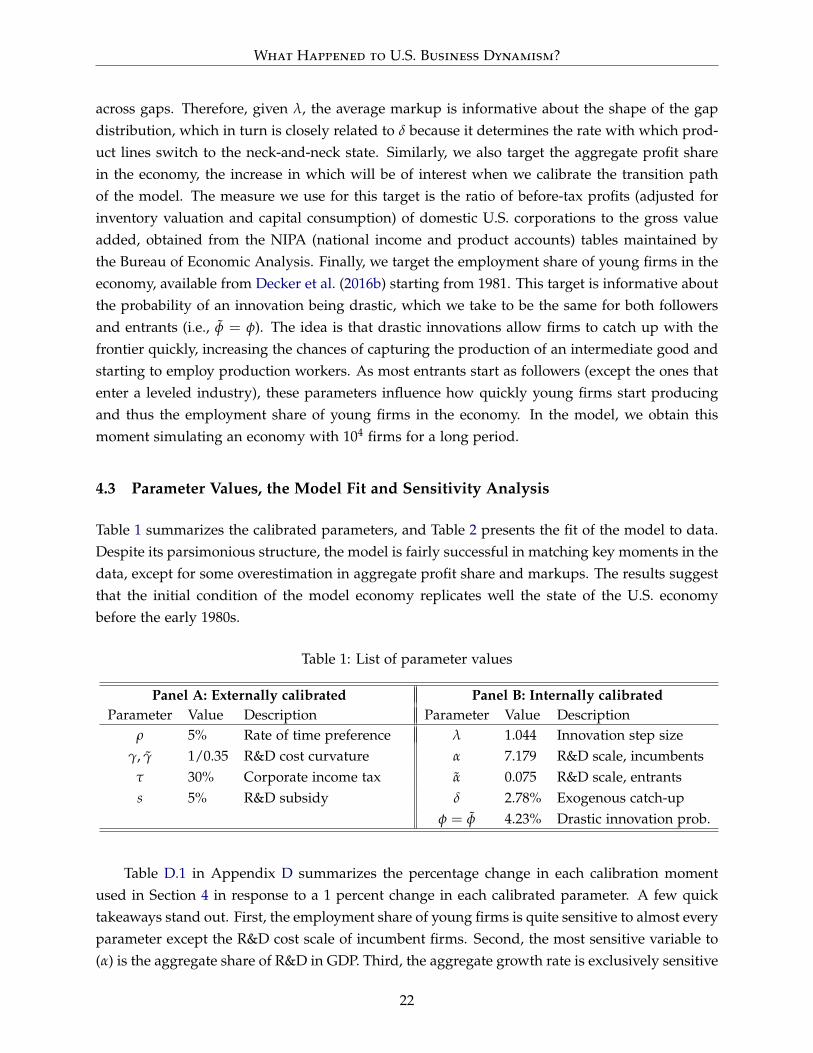
Table 1 summarizes the calibrated parameters, and Table 2 presents the fit of the model to data.Despite its parsimonious structure, the model is fairly successful in matching key moments in thedata, except for some overestimation in aggregate profit share and markups. The results suggestthat the initial condition of the model economy replicates well the state of the U.S. economybefore the early 1980s.
Table 1: List of parameter values
Panel A: Externally calibrated Panel B: Internally calibratedParameter Value Description Parameter Value Description
ρ 5% Rate of time preference λ 1.044 Innovation step sizeγ, γ 1/0.35 R&D cost curvature α 7.179 R&D scale, incumbents
τ 30% Corporate income tax α 0.075 R&D scale, entrantss 5% R&D subsidy δ 2.78% Exogenous catch-up
φ = φ 4.23% Drastic innovation prob.
Table D.1 in Appendix D summarizes the percentage change in each calibration momentused in Section 4 in response to a 1 percent change in each calibrated parameter. A few quicktakeaways stand out. First, the employment share of young firms is quite sensitive to almost everyparameter except the R&D cost scale of incumbent firms. Second, the most sensitive variable to(α) is the aggregate share of R&D in GDP. Third, the aggregate growth rate is exclusively sensitive
22
What Happened to U.S. Business Dynamism?
Table 2: Model fit
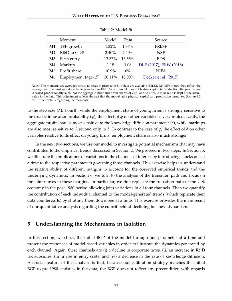
Moment Model Data Source
M1 TFP growth 1.32% 1.37% FRBSFM2 R&D to GDP 2.40% 2.40% NSFM3 Firm entry 13.57% 13.55% BDSM4 Markup 1.18 1.08 DLE (2017), ERW (2018)M5 Profit share 10.9% 6% NIPAM6 Employment (age<5) 20.11% 18.00% Decker et al. (2015)
Notes: The moments are averages across to decades prior to 1981 if data are available (M1,M2,M4,M5); if not, they reflect theaverage over the most recent available years before 1981. As our model does not feature capital in production, the profit shareis scaled proportionally such that the aggregate labor and profit shares of GDP add to 1 while their ratio is kept at the actualvalue in the data. This adjustment reflects the fact that the model lacks physical capital as a productive input. See Section 4.2for further details regarding the moments.
to the step size (λ). Fourth, while the employment share of young firms is strongly sensitive tothe drastic innovation probability (φ), the effect of φ on other variables is very muted. Lastly, theaggregate profit share is most sensitive to the knowledge diffusion parameter (δ), while markupsare also most sensitive to δ, second only to λ. In contrast to the case of φ, the effect of δ on othervariables relative to its effect on young firms’ employment share is also much stronger.
In the next two sections, we use our model to investigate potential mechanisms that may havecontributed to the empirical trends discussed in Section 2. We proceed in two steps. In Section 5,we illustrate the implications of variations in the channels of interest by introducing shocks one ata time to the respective parameters governing those channels. This exercise helps us understandthe relative ability of different margins to account for the observed empirical trends and theunderlying dynamics. In Section 6, we turn to the analysis of the transition path and focus onthe joint moves in these margins. In particular, we first replicate the transition path of the U.S.economy in the post-1980 period allowing joint variations in all four channels. Then we quantifythe contribution of each individual channel to the model-generated trends (which replicate theirdata counterparts) by shutting them down one at a time. This exercise provides the main resultof our quantitative analysis regarding the culprit behind declining business dynamism.
5 Understanding the Mechanisms in Isolation
In this section, we shock the initial BGP of the model through one parameter at a time andpresent the responses of model-based variables in order to illustrate the dynamics generated byeach channel. Again, these channels are (i) a decline in corporate taxes, (ii) an increase in R&Dtax subsidies, (iii) a rise in entry costs, and (iv) a decrease in the rate of knowledge diffusion.A crucial feature of this analysis is that, because our calibration strategy matches the initialBGP to pre-1980 statistics in the data, the BGP does not reflect any precondition with regards
23
What Happened to U.S. Business Dynamism?
to the empirical trends that we analyze later. Therefore, our model-based responses will almostexclusively rely on information that predates the shifts in the U.S. business environment, whichwe aim at explaining here, with the minimal exceptions clarified later. In other words, theexercise will reflect only minimal information from the observed dynamics of declining businessdynamism. Nevertheless, as we shall see next, the response of the model to a decline in theintensity of knowledge diffusion tracks the empirical trends quite closely.
Our approach is to introduce a path of shocks to {αt, δt, τt, st} one at a time. We assumethat each change takes place over a period of 30 years, accounting for the three decades between1980 and 2010. We specify the paths of shocks as follows. In the data, the corporate income taxrate decreases from 30% to 20%, and R&D subsidies increase from 5% to 20% (see Section 6.1for further details). To demonstrate the strengths and weaknesses of these channels, we considerlarger moves: a drop to 0 percent for corporate tax rates and a an increase to 50 percent in R&Dsubsidies in linear fashion.
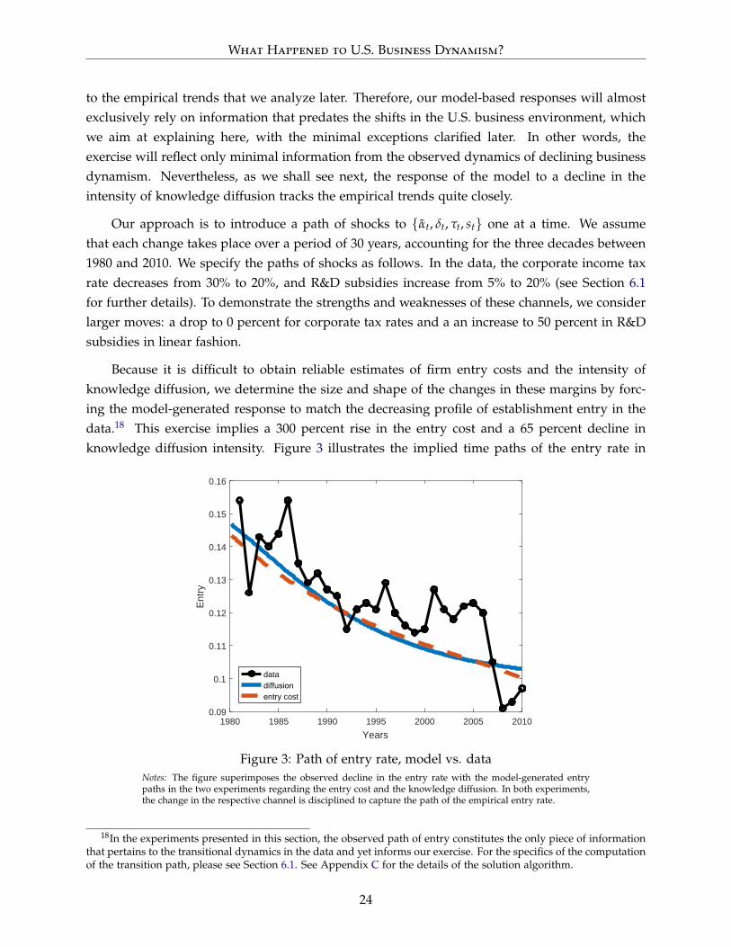
Because it is difficult to obtain reliable estimates of firm entry costs and the intensity ofknowledge diffusion, we determine the size and shape of the changes in these margins by forc-ing the model-generated response to match the decreasing profile of establishment entry in thedata.18 This exercise implies a 300 percent rise in the entry cost and a 65 percent decline inknowledge diffusion intensity. Figure 3 illustrates the implied time paths of the entry rate in
1980 1985 1990 1995 2000 2005 2010
Years
0.09
0.1
0.11
0.12
0.13
0.14
0.15
0.16
Ent
ry
datadiffusionentry cost
Figure 3: Path of entry rate, model vs. dataNotes: The figure superimposes the observed decline in the entry rate with the model-generated entrypaths in the two experiments regarding the entry cost and the knowledge diffusion. In both experiments,the change in the respective channel is disciplined to capture the path of the empirical entry rate.
18In the experiments presented in this section, the observed path of entry constitutes the only piece of informationthat pertains to the transitional dynamics in the data and yet informs our exercise. For the specifics of the computationof the transition path, please see Section 6.1. See Appendix C for the details of the solution algorithm.
24
What Happened to U.S. Business Dynamism?
these two experiments, superimposed with their counterpart in the data. The figure demon-strates the success of the individual channels in generating the decline in entry observed in thedata.
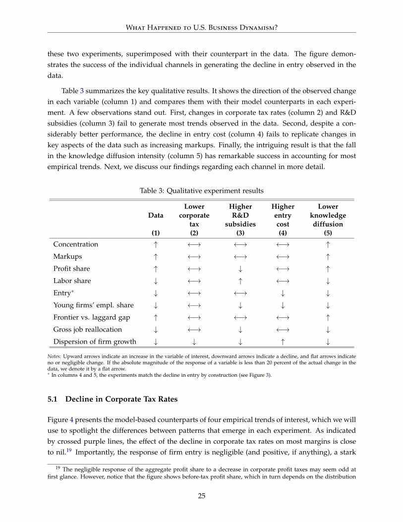
Table 3 summarizes the key qualitative results. It shows the direction of the observed changein each variable (column 1) and compares them with their model counterparts in each experi-ment. A few observations stand out. First, changes in corporate tax rates (column 2) and R&Dsubsidies (column 3) fail to generate most trends observed in the data. Second, despite a con-siderably better performance, the decline in entry cost (column 4) fails to replicate changes inkey aspects of the data such as increasing markups. Finally, the intriguing result is that the fallin the knowledge diffusion intensity (column 5) has remarkable success in accounting for mostempirical trends. Next, we discuss our findings regarding each channel in more detail.
Table 3: Qualitative experiment results
Data
(1)
Lowercorporate
tax(2)
HigherR&D
subsidies(3)
Higherentrycost(4)
Lowerknowledgediffusion
(5)
Concentration ↑ ←→ ←→ ←→ ↑Markups ↑ ←→ ←→ ←→ ↑Profit share ↑ ←→ ↓ ←→ ↑Labor share ↓ ←→ ↑ ←→ ↓Entry∗ ↓ ←→ ←→ ↓ ↓Young firms’ empl. share ↓ ←→ ↓ ↓ ↓Frontier vs. laggard gap ↑ ←→ ←→ ←→ ↑Gross job reallocation ↓ ←→ ↓ ←→ ↓Dispersion of firm growth ↓ ↓ ↓ ↑ ↓
Notes: Upward arrows indicate an increase in the variable of interest, downward arrows indicate a decline, and flat arrows indicateno or negligible change. If the absolute magnitude of the response of a variable is less than 20 percent of the actual change in thedata, we denote it by a flat arrow.∗ In columns 4 and 5, the experiments match the decline in entry by construction (see Figure 3).
5.1 Decline in Corporate Tax Rates
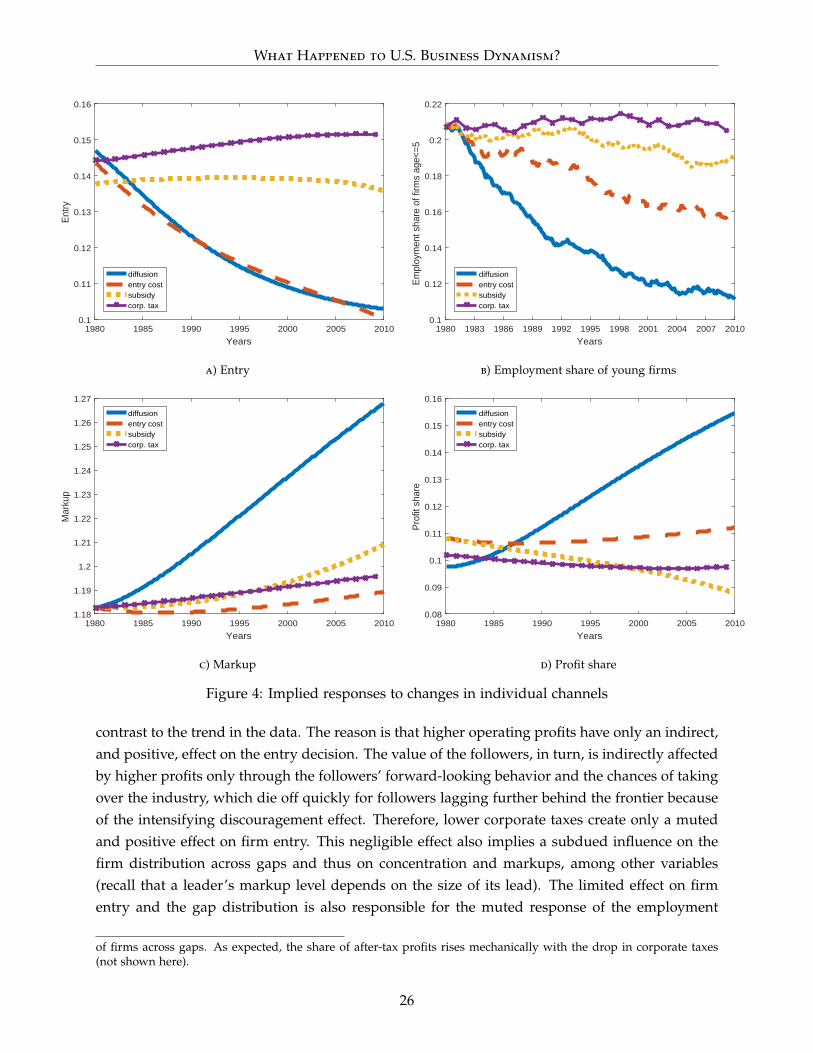
Figure 4 presents the model-based counterparts of four empirical trends of interest, which we willuse to spotlight the differences between patterns that emerge in each experiment. As indicatedby crossed purple lines, the effect of the decline in corporate tax rates on most margins is closeto nil.19 Importantly, the response of firm entry is negligible (and positive, if anything), a stark
19 The negligible response of the aggregate profit share to a decrease in corporate profit taxes may seem odd atfirst glance. However, notice that the figure shows before-tax profit share, which in turn depends on the distribution
25
What Happened to U.S. Business Dynamism?
1980 1985 1990 1995 2000 2005 2010
Years
0.1
0.11
0.12
0.13
0.14
0.15
0.16
Ent
ry
diffusionentry costsubsidycorp. tax
a) Entry
1980 1983 1986 1989 1992 1995 1998 2001 2004 2007 2010
Years
0.1
0.12
0.14
0.16
0.18
0.2
0.22
Em
ploy
men
t sha
re o
f firm
s ag
e<=5
diffusionentry costsubsidycorp. tax
b) Employment share of young firms
1980 1985 1990 1995 2000 2005 2010
Years
1.18
1.19
1.2
1.21
1.22
1.23
1.24
1.25
1.26
1.27
Mar
kup
diffusionentry costsubsidycorp. tax
c) Markup
1980 1985 1990 1995 2000 2005 2010
Years
0.08
0.09
0.1
0.11
0.12
0.13
0.14
0.15
0.16
Pro
fit s
hare
diffusionentry costsubsidycorp. tax
d) Profit share
Figure 4: Implied responses to changes in individual channels
contrast to the trend in the data. The reason is that higher operating profits have only an indirect,and positive, effect on the entry decision. The value of the followers, in turn, is indirectly affectedby higher profits only through the followers’ forward-looking behavior and the chances of takingover the industry, which die off quickly for followers lagging further behind the frontier becauseof the intensifying discouragement effect. Therefore, lower corporate taxes create only a mutedand positive effect on firm entry. This negligible effect also implies a subdued influence on thefirm distribution across gaps and thus on concentration and markups, among other variables(recall that a leader’s markup level depends on the size of its lead). The limited effect on firmentry and the gap distribution is also responsible for the muted response of the employment
of firms across gaps. As expected, the share of after-tax profits rises mechanically with the drop in corporate taxes(not shown here).
26
What Happened to U.S. Business Dynamism?
share of young firms and other variables listed in column 2 of Table 3.
5.2 Increase in R&D Subsidies
In Figure 4, the dotted yellow lines denote the responses to the increase in R&D subsidies. Al-though the responses to the increase in R&D subsidies are slightly stronger, they are still very faraway from the empirical patterns, most crucially in the case of firm entry. The increase in innova-tive activity affects firms’ distribution across gaps, moving some variables such as markups andthe employment share of young firms (and gross job reallocation, to some extent) in the right di-rection, although the magnitude of the changes is very limited. Moreover, the profit share of GDPdeclines counterfactually. This result may appear at odds with the pickup in markups, but therationale is as follows. The profit share of GDP is slightly different than the average (operational)profitability of firms, which would reflect only the distributional changes and move, therefore,in parallel to markups. However, the profit share of GDP is related to the aggregate labor share,which reflects the wage level in the economy. With higher R&D subsidies, the demand of leadingfirms for R&D employment increases, pushing up the wage level in the economy. Reciprocally,the profit share of GDP decreases. Higher wages also imply a higher cost of entry, which drivesthe slight decline in the entry rate.
5.3 Increase in Entry Costs
As described earlier, the increase in entry costs analyzed here is such that the response of firmentry matches the empirical pattern. Therefore, it is no surprise that in Figure 4a the model-generated entry rate (dashed red line) closely follows its empirical counterpart, with entry beingdiscouraged by higher costs of entry innovation. In contrast to the tax and subsidy experiments,the decline in entry costs is able to generate a modest fall in the employment share of youngfirms, as lower firm entry implies lower supply of new and young firms.
Despite some success in capturing entry and young firm dynamics, the rise in entry costfails to generate any significant move in markups and the profit share. The main reason for theseresults is that a fall in entry itself does not alter incumbent incentives to a degree that can causea large enough shift in the distribution of firms toward larger gaps. On the contrary, the share ofleveled sectors increases mildly, as reflected by the counterfactual decline in market concentration(column 4 in Table 3). The mechanics behind this result is as follows. Lower entry implies a lowerchurning for the follower firms, damping the negative business stealing effect exerted by entryon the innovation incentives of followers. This lower churning rate, in turn, boosts innovation bythe followers, increasing the share of leveled sectors and thus pushing down concentration. Butthis shift loses steam over time, allowing the sectoral distribution to move slightly toward largergaps, which causes some pickup in markups and the profit share, albeit a very small one. The
27
What Happened to U.S. Business Dynamism?
weak distributional response is also responsible for the experiment’s failure to replicate otherpatterns such as gross job reallocation.
5.4 Decline in Knowledge Diffusion
Similar to the previous experiment, the pattern that we introduce for the decline in knowledgediffusion is such that the model response in firm entry matches the empirical pattern, with thelower catch-up probability decreasing the value of being a follower and thus the benefit forentry. In stark contrast to the previous experiments, however, the decline in knowledge diffusionsucceeds in generating reasonable variations in all margins in correct directions (indicated bysolid blue lines). Average markup and the profit share of GDP rise dramatically, while the declinein the employment share of young firms is the strongest. Moreover, as shown in the last columnof Table 3, aggregate labor share decreases as well, a feature that all previous experiments miss.In addition, both gross job reallocation and the standard deviation of firm growth decline in linewith the empirical regularities.
The crux of this experiment lies in the shift of the gap distribution to larger gaps induced bythe decline in knowledge diffusion. The decline in δ decreases the intensity with which leaders ofany lead find themselves in a neck-and-neck position, thus resulting in larger masses of productlines across relatively larger gap differences. This shift induces higher concentration, averagemarkups, and profit share. Less catch-up also leads to less job reallocation and a fall in firmgrowth dispersion. Moreover, with lower knowledge diffusion, the process of new (and thereforeyoung) firms, which start the business replacing followers, taking over production slows down,resulting in a lower employment share of young firms in the economy. Notice that the decline inthis margin is larger than in the experiment of higher entry costs, even though the magnitude ofthe drop in the entry rate is almost the same in both experiments. A stronger response occurs inthis exercise because of the additional negative effect of lower knowledge diffusion, decreasingthe intensity with which young followers catch up with the leaders and eventually take over theproduction.
Overall, these model responses imply that a decline in knowledge diffusion stands out as alikely suspect behind the decline in U.S. business dynamism. In order to assess quantitativelywhether this was actually the case, we next turn to the analysis where we let these four forces bejointly at play and quantify their relative importance.
6 Investigation of Joint Forces
The channels we consider here have been moving simultaneously over the years. For exam-ple, changes in corporate tax policies and the introduction of R&D subsidies were major policy
28
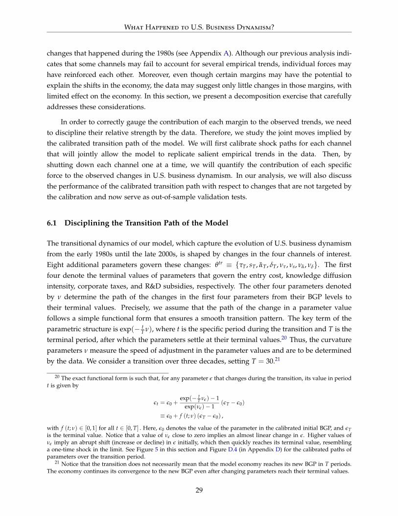
What Happened to U.S. Business Dynamism?
changes that happened during the 1980s (see Appendix A). Although our previous analysis indi-cates that some channels may fail to account for several empirical trends, individual forces mayhave reinforced each other. Moreover, even though certain margins may have the potential toexplain the shifts in the economy, the data may suggest only little changes in those margins, withlimited effect on the economy. In this section, we present a decomposition exercise that carefullyaddresses these considerations.
In order to correctly gauge the contribution of each margin to the observed trends, we needto discipline their relative strength by the data. Therefore, we study the joint moves implied bythe calibrated transition path of the model. We will first calibrate shock paths for each channelthat will jointly allow the model to replicate salient empirical trends in the data. Then, byshutting down each channel one at a time, we will quantify the contribution of each specificforce to the observed changes in U.S. business dynamism. In our analysis, we will also discussthe performance of the calibrated transition path with respect to changes that are not targeted bythe calibration and now serve as out-of-sample validation tests.
6.1 Disciplining the Transition Path of the Model
The transitional dynamics of our model, which capture the evolution of U.S. business dynamismfrom the early 1980s until the late 2000s, is shaped by changes in the four channels of interest.Eight additional parameters govern these changes: θtr ≡ {τT, sT, αT, δT, ντ, νs, να, νδ}. The firstfour denote the terminal values of parameters that govern the entry cost, knowledge diffusionintensity, corporate taxes, and R&D subsidies, respectively. The other four parameters denotedby ν determine the path of the changes in the first four parameters from their BGP levels totheir terminal values. Precisely, we assume that the path of the change in a parameter valuefollows a simple functional form that ensures a smooth transition pattern. The key term of theparametric structure is exp(− t
T ν), where t is the specific period during the transition and T is theterminal period, after which the parameters settle at their terminal values.20 Thus, the curvatureparameters ν measure the speed of adjustment in the parameter values and are to be determinedby the data. We consider a transition over three decades, setting T = 30.21
20 The exact functional form is such that, for any parameter ε that changes during the transition, its value in periodt is given by
εt = ε0 +exp(− t
T νε)− 1exp(νε)− 1
(εT − ε0)
≡ ε0 + f (t; ν) (εT − ε0) ,
with f (t; ν) ∈ [0, 1] for all t ∈ [0, T] . Here, ε0 denotes the value of the parameter in the calibrated initial BGP, and εTis the terminal value. Notice that a value of νε close to zero implies an almost linear change in ε. Higher values ofνε imply an abrupt shift (increase or decline) in ε initially, which then quickly reaches its terminal value, resemblinga one-time shock in the limit. See Figure 5 in this section and Figure D.4 (in Appendix D) for the calibrated paths ofparameters over the transition period.
21 Notice that the transition does not necessarily mean that the model economy reaches its new BGP in T periods.The economy continues its convergence to the new BGP even after changing parameters reach their terminal values.
29
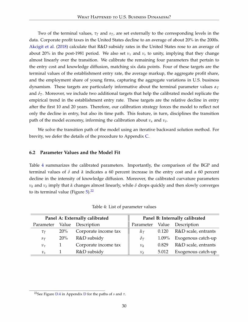
What Happened to U.S. Business Dynamism?
Two of the terminal values, τT and sT, are set externally to the corresponding levels in thedata. Corporate profit taxes in the United States decline to an average of about 20% in the 2000s.Akcigit et al. (2018) calculate that R&D subsidy rates in the United States rose to an average ofabout 20% in the post-1981 period. We also set ντ and νs to unity, implying that they changealmost linearly over the transition. We calibrate the remaining four parameters that pertain tothe entry cost and knowledge diffusion, matching six data points. Four of these targets are theterminal values of the establishment entry rate, the average markup, the aggregate profit share,and the employment share of young firms, capturing the aggregate variations in U.S. businessdynamism. These targets are particularly informative about the terminal parameter values αT
and δT. Moreover, we include two additional targets that help the calibrated model replicate theempirical trend in the establishment entry rate. These targets are the relative decline in entryafter the first 10 and 20 years. Therefore, our calibration strategy forces the model to reflect notonly the decline in entry, but also its time path. This feature, in turn, disciplines the transitionpath of the model economy, informing the calibration about να and νδ.
We solve the transition path of the model using an iterative backward solution method. Forbrevity, we defer the details of the procedure to Appendix C.
6.2 Parameter Values and the Model Fit
Table 4 summarizes the calibrated parameters. Importantly, the comparison of the BGP andterminal values of δ and α indicates a 60 percent increase in the entry cost and a 60 percentdecline in the intensity of knowledge diffusion. Moreover, the calibrated curvature parametersνα and νδ imply that α changes almost linearly, while δ drops quickly and then slowly convergesto its terminal value (Figure 5).22
Table 4: List of parameter values
Panel A: Externally calibrated Panel B: Internally calibratedParameter Value Description Parameter Value Description
τT 20% Corporate income tax αT 0.120 R&D scale, entrantssT 20% R&D subsidy δT 1.09% Exogenous catch-upντ 1 Corporate income tax να 0.829 R&D scale, entrantsνs 1 R&D subsidy νδ 5.012 Exogenous catch-up
22See Figure D.4 in Appendix D for the paths of s and τ.
30
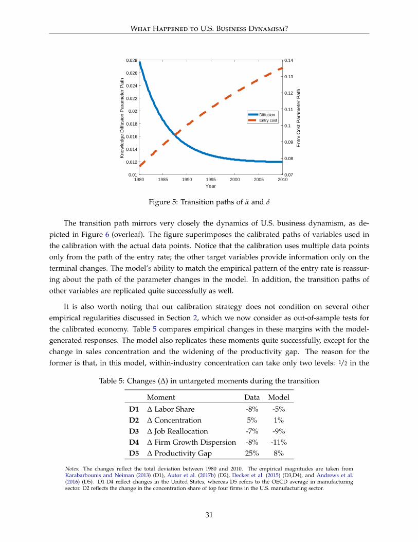
What Happened to U.S. Business Dynamism?
1980 1985 1990 1995 2000 2005 2010
Year
0.01
0.012
0.014
0.016
0.018
0.02
0.022
0.024
0.026
0.028
Kno
wle
dge
Diff
usio
n P
aram
eter
Pat
h
0.07
0.08
0.09
0.1
0.11
0.12
0.13
0.14
Ent
ry C
ost P
aram
eter
Pat
h
DiffusionEntry cost
Figure 5: Transition paths of α and δ
The transition path mirrors very closely the dynamics of U.S. business dynamism, as de-picted in Figure 6 (overleaf). The figure superimposes the calibrated paths of variables used inthe calibration with the actual data points. Notice that the calibration uses multiple data pointsonly from the path of the entry rate; the other target variables provide information only on theterminal changes. The model’s ability to match the empirical pattern of the entry rate is reassur-ing about the path of the parameter changes in the model. In addition, the transition paths ofother variables are replicated quite successfully as well.
It is also worth noting that our calibration strategy does not condition on several otherempirical regularities discussed in Section 2, which we now consider as out-of-sample tests forthe calibrated economy. Table 5 compares empirical changes in these margins with the model-generated responses. The model also replicates these moments quite successfully, except for thechange in sales concentration and the widening of the productivity gap. The reason for theformer is that, in this model, within-industry concentration can take only two levels: 1/2 in the
Table 5: Changes (∆) in untargeted moments during the transition
Moment Data Model
D1 ∆ Labor Share -8% -5%D2 ∆ Concentration 5% 1%D3 ∆ Job Reallocation -7% -9%D4 ∆ Firm Growth Dispersion -8% -11%D5 ∆ Productivity Gap 25% 8%
Notes: The changes reflect the total deviation between 1980 and 2010. The empirical magnitudes are taken fromKarabarbounis and Neiman (2013) (D1), Autor et al. (2017b) (D2), Decker et al. (2015) (D3,D4), and Andrews et al.(2016) (D5). D1-D4 reflect changes in the United States, whereas D5 refers to the OECD average in manufacturingsector. D2 reflects the change in the concentration share of top four firms in the U.S. manufacturing sector.
31
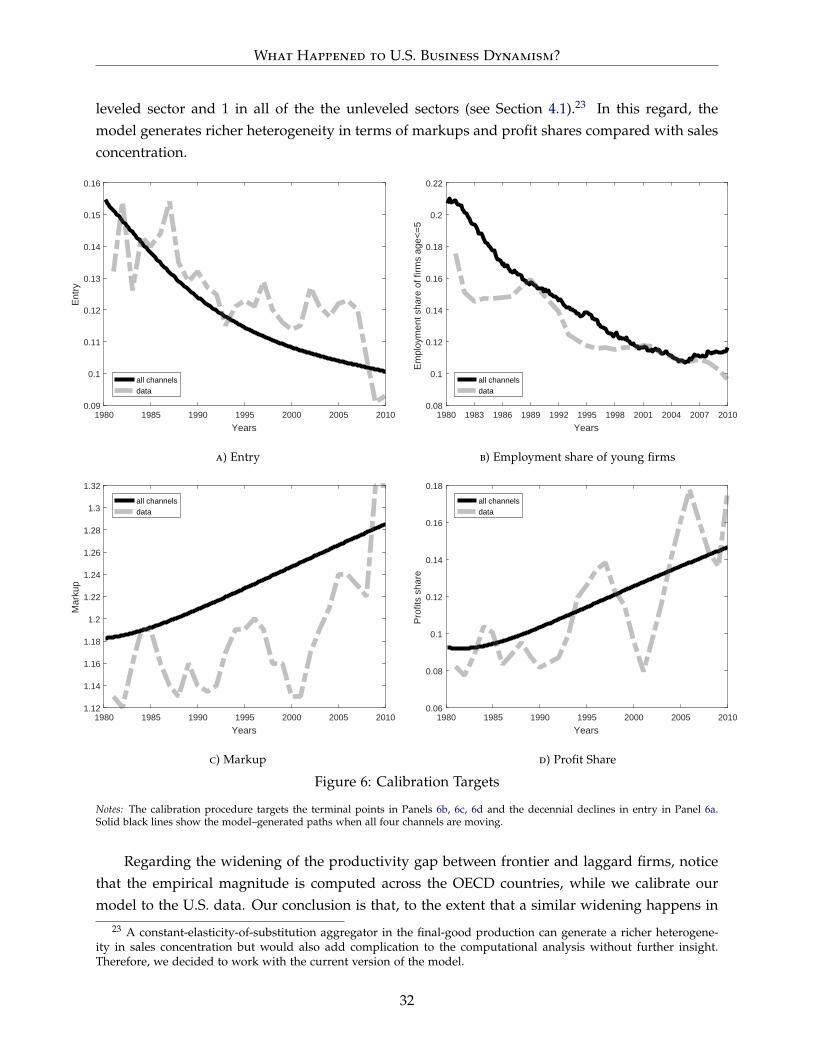
What Happened to U.S. Business Dynamism?
leveled sector and 1 in all of the the unleveled sectors (see Section 4.1).23 In this regard, themodel generates richer heterogeneity in terms of markups and profit shares compared with salesconcentration.
1980 1985 1990 1995 2000 2005 2010
Years
0.09
0.1
0.11
0.12
0.13
0.14
0.15
0.16
Ent
ry
all channelsdata
a) Entry
1980 1983 1986 1989 1992 1995 1998 2001 2004 2007 2010
Years
0.08
0.1
0.12
0.14
0.16
0.18
0.2
0.22
Em
ploy
men
t sha
re o
f firm
s ag
e<=
5
all channelsdata
b) Employment share of young firms
1980 1985 1990 1995 2000 2005 2010
Years
1.12
1.14
1.16
1.18
1.2
1.22
1.24
1.26
1.28
1.3
1.32
Mar
kup
all channelsdata
c) Markup
1980 1985 1990 1995 2000 2005 2010
Years
0.06
0.08
0.1
0.12
0.14
0.16
0.18
Pro
fits
shar
e
all channelsdata
d) Profit Share
Figure 6: Calibration Targets
Notes: The calibration procedure targets the terminal points in Panels 6b, 6c, 6d and the decennial declines in entry in Panel 6a.Solid black lines show the model–generated paths when all four channels are moving.
Regarding the widening of the productivity gap between frontier and laggard firms, noticethat the empirical magnitude is computed across the OECD countries, while we calibrate ourmodel to the U.S. data. Our conclusion is that, to the extent that a similar widening happens in
23 A constant-elasticity-of-substitution aggregator in the final-good production can generate a richer heterogene-ity in sales concentration but would also add complication to the computational analysis without further insight.Therefore, we decided to work with the current version of the model.
32
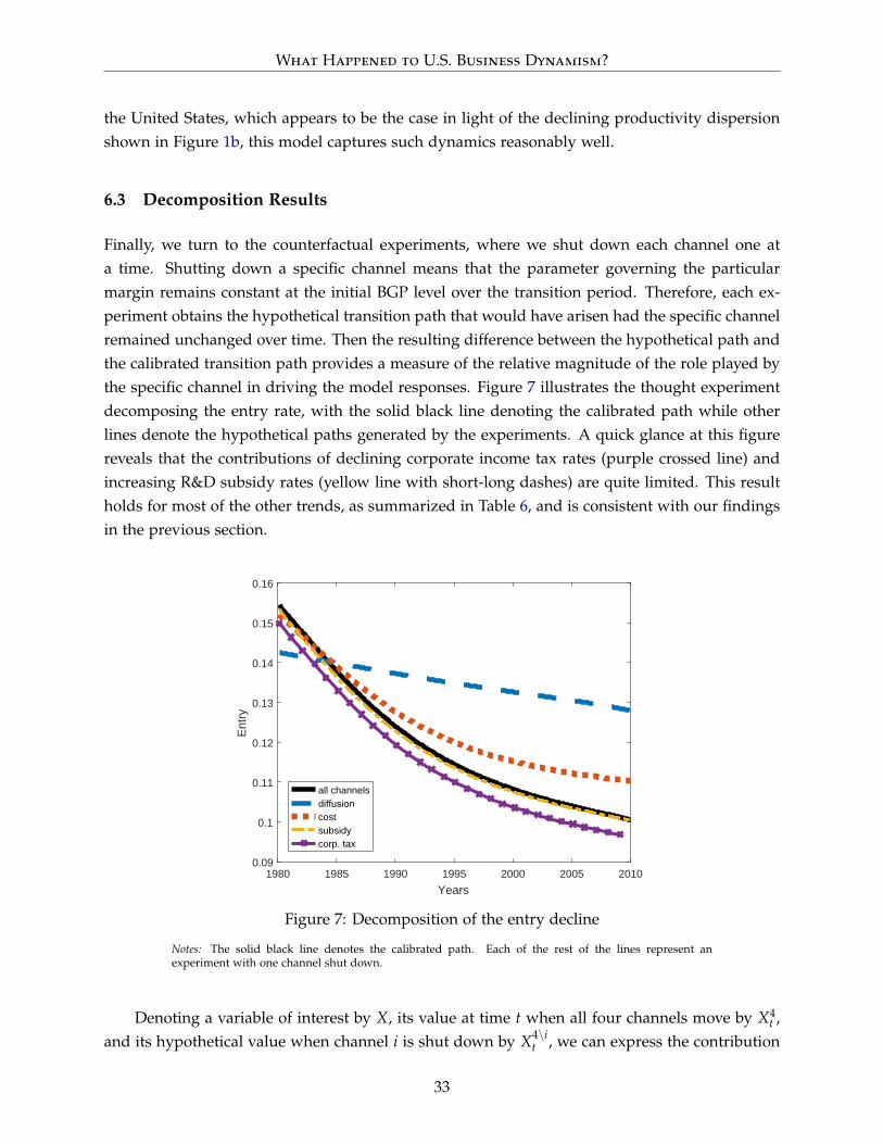
What Happened to U.S. Business Dynamism?
the United States, which appears to be the case in light of the declining productivity dispersionshown in Figure 1b, this model captures such dynamics reasonably well.
6.3 Decomposition Results
Finally, we turn to the counterfactual experiments, where we shut down each channel one ata time. Shutting down a specific channel means that the parameter governing the particularmargin remains constant at the initial BGP level over the transition period. Therefore, each ex-periment obtains the hypothetical transition path that would have arisen had the specific channelremained unchanged over time. Then the resulting difference between the hypothetical path andthe calibrated transition path provides a measure of the relative magnitude of the role played bythe specific channel in driving the model responses. Figure 7 illustrates the thought experimentdecomposing the entry rate, with the solid black line denoting the calibrated path while otherlines denote the hypothetical paths generated by the experiments. A quick glance at this figurereveals that the contributions of declining corporate income tax rates (purple crossed line) andincreasing R&D subsidy rates (yellow line with short-long dashes) are quite limited. This resultholds for most of the other trends, as summarized in Table 6, and is consistent with our findingsin the previous section.
1980 1985 1990 1995 2000 2005 2010
Years
0.09
0.1
0.11
0.12
0.13
0.14
0.15
0.16
Ent
ry
all channelsdiffusioncostsubsidycorp. tax
Figure 7: Decomposition of the entry decline
Notes: The solid black line denotes the calibrated path. Each of the rest of the lines represent anexperiment with one channel shut down.
Denoting a variable of interest by X, its value at time t when all four channels move by X4t ,
and its hypothetical value when channel i is shut down by X4\it , we can express the contribution
33
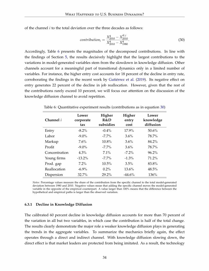
What Happened to U.S. Business Dynamism?
of the channel i to the total deviation over the three decades as follows:
contributioni =X4
2010 − X4\i2010
X42010 − X4
1980. (30)
Accordingly, Table 6 presents the magnitudes of the decomposed contributions. In line withthe findings of Section 5, the results decisively highlight that the largest contributions to thevariations in model-generated variables stem from the slowdown in knowledge diffusion. Otherchannels account for a meaningful part of transitional dynamics only in a limited number ofvariables. For instance, the higher entry cost accounts for 18 percent of the decline in entry rate,corroborating the findings in the recent work by Gutiérrez et al. (2019). Its negative effect onentry generates 22 percent of the decline in job reallocation. However, given that the rest ofthe contributions rarely exceed 10 percent, we will focus our attention on the discussion of theknowledge diffusion channel to avoid repetition.
Table 6: Quantitative experiment results (contributions as in equation 30)
Channel iLower
corporatetax
HigherR&D
subsidies
Higherentrycost
Lowerknowledgediffusion
Entry -8.2% -0.4% 17.9% 50.6%Labor -9.0% -7.7% 3.6% 78.7%Markup 7.6% 10.8% 3.6% 84.2%Profit -9.0% -7.7% 3.6% 78.7%Concentration 4.3% 7.1% -7.2% 96.2%Young firms -13.2% -7.7% -1.3% 71.2%Prod. gap 7.2% 10.5% 3.5% 83.8%Reallocation -6.9% 0.2% 13.6% 48.5%Dispersion 32.7% 29.2% -44.6% 136%
Notes: Percentage values measure the share of the contribution from the specific channel to the total model-generateddeviation between 1980 and 2010. Negative values mean that adding the specific channel moves the model-generatedvariable in the opposite of the empirical counterpart. A value larger than 100% means that the difference between thehypothetical and empirical paths is larger than the observed variation.
6.3.1 Decline in Knowledge Diffusion
The calibrated 60 percent decline in knowledge diffusion accounts for more than 70 percent ofthe variation in all but two variables, in which case the contribution is half of the total change.The results clearly demonstrate the major role a weaker knowledge diffusion plays in generatingthe trends in the aggregate variables. To summarize the mechanics briefly again, the effectoperates through a direct and indirect channel. With knowledge diffusion slowing down, thedirect effect is that market leaders are protected from being imitated. As a result, the technology
34
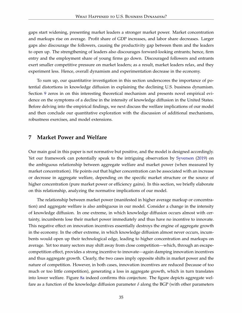
What Happened to U.S. Business Dynamism?
gaps start widening, presenting market leaders a stronger market power. Market concentrationand markups rise on average. Profit share of GDP increases, and labor share decreases. Largergaps also discourage the followers, causing the productivity gap between them and the leadersto open up. The strengthening of leaders also discourages forward-looking entrants; hence, firmentry and the employment share of young firms go down. Discouraged followers and entrantsexert smaller competitive pressure on market leaders; as a result, market leaders relax, and theyexperiment less. Hence, overall dynamism and experimentation decrease in the economy.
To sum up, our quantitative investigation in this section underscores the importance of po-tential distortions in knowledge diffusion in explaining the declining U.S. business dynamism.Section 9 zeros in on this interesting theoretical mechanism and presents novel empirical evi-dence on the symptoms of a decline in the intensity of knowledge diffusion in the United States.Before delving into the empirical findings, we next discuss the welfare implications of our modeland then conclude our quantitative exploration with the discussion of additional mechanisms,robustness exercises, and model extensions.
7 Market Power and Welfare
Our main goal in this paper is not normative but positive, and the model is designed accordingly.Yet our framework can potentially speak to the intriguing observation by Syverson (2019) onthe ambiguous relationship between aggregate welfare and market power (when measured bymarket concentration). He points out that higher concentration can be associated with an increaseor decrease in aggregate welfare, depending on the specific market structure or the source ofhigher concentration (pure market power or efficiency gains). In this section, we briefly elaborateon this relationship, analyzing the normative implications of our model.
The relationship between market power (manifested in higher average markup or concentra-tion) and aggregate welfare is also ambiguous in our model. Consider a change in the intensityof knowledge diffusion. In one extreme, in which knowledge diffusion occurs almost with cer-tainty, incumbents lose their market power immediately and thus have no incentive to innovate.This negative effect on innovation incentives essentially destroys the engine of aggregate growthin the economy. In the other extreme, in which knowledge diffusion almost never occurs, incum-bents would open up their technological edge, leading to higher concentration and markups onaverage. Yet too many sectors may shift away from close competition—which, through an escape-competition effect, provides a strong incentive to innovate—again damping innovation incentivesand thus aggregate growth. Clearly, the two cases imply opposite shifts in market power and thenature of competition. However, in both cases, innovation incentives are reduced (because of toomuch or too little competition), generating a loss in aggregate growth, which in turn translatesinto lower welfare. Figure 8a indeed confirms this conjecture. The figure depicts aggregate wel-fare as a function of the knowledge diffusion parameter δ along the BGP (with other parameters
35
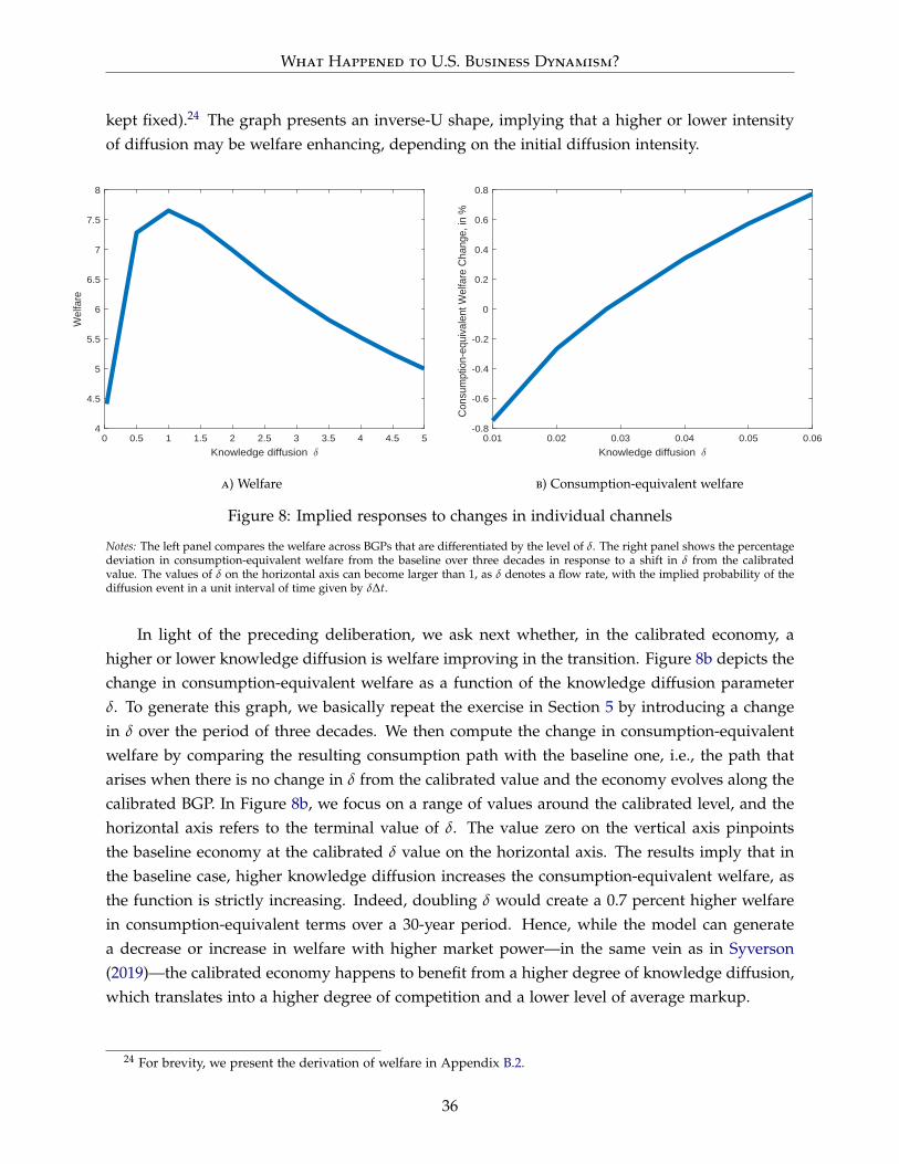
What Happened to U.S. Business Dynamism?
kept fixed).24 The graph presents an inverse-U shape, implying that a higher or lower intensityof diffusion may be welfare enhancing, depending on the initial diffusion intensity.
0 0.5 1 1.5 2 2.5 3 3.5 4 4.5 5
Knowledge diffusion /
4
4.5
5
5.5
6
6.5
7
7.5
8
Wel
fare
a) Welfare
0.01 0.02 0.03 0.04 0.05 0.06
Knowledge diffusion /
-0.8
-0.6
-0.4
-0.2
0
0.2
0.4
0.6
0.8
Con
sum
ptio
n-eq
uiva
lent
Wel
fare
Cha
nge,
in %
b) Consumption-equivalent welfare
Figure 8: Implied responses to changes in individual channels
Notes: The left panel compares the welfare across BGPs that are differentiated by the level of δ. The right panel shows the percentagedeviation in consumption-equivalent welfare from the baseline over three decades in response to a shift in δ from the calibratedvalue. The values of δ on the horizontal axis can become larger than 1, as δ denotes a flow rate, with the implied probability of thediffusion event in a unit interval of time given by δ∆t.
In light of the preceding deliberation, we ask next whether, in the calibrated economy, ahigher or lower knowledge diffusion is welfare improving in the transition. Figure 8b depicts thechange in consumption-equivalent welfare as a function of the knowledge diffusion parameterδ. To generate this graph, we basically repeat the exercise in Section 5 by introducing a changein δ over the period of three decades. We then compute the change in consumption-equivalentwelfare by comparing the resulting consumption path with the baseline one, i.e., the path thatarises when there is no change in δ from the calibrated value and the economy evolves along thecalibrated BGP. In Figure 8b, we focus on a range of values around the calibrated level, and thehorizontal axis refers to the terminal value of δ. The value zero on the vertical axis pinpointsthe baseline economy at the calibrated δ value on the horizontal axis. The results imply that inthe baseline case, higher knowledge diffusion increases the consumption-equivalent welfare, asthe function is strictly increasing. Indeed, doubling δ would create a 0.7 percent higher welfarein consumption-equivalent terms over a 30-year period. Hence, while the model can generatea decrease or increase in welfare with higher market power—in the same vein as in Syverson(2019)—the calibrated economy happens to benefit from a higher degree of knowledge diffusion,which translates into a higher degree of competition and a lower level of average markup.
24 For brevity, we present the derivation of welfare in Appendix B.2.
36
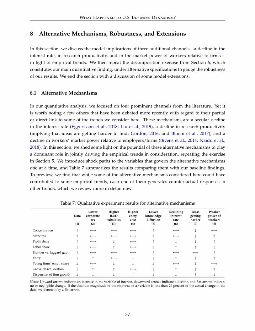
What Happened to U.S. Business Dynamism?
8 Alternative Mechanisms, Robustness, and Extensions
In this section, we discuss the model implications of three additional channels—a decline in theinterest rate, in research productivity, and in the market power of workers relative to firms—in light of empirical trends. We then repeat the decomposition exercise from Section 6, whichconstitutes our main quantitative finding, under alternative specifications to gauge the robustnessof our results. We end the section with a discussion of some model extensions.
8.1 Alternative Mechanisms
In our quantitative analysis, we focused on four prominent channels from the literature. Yet itis worth noting a few others that have been debated more recently with regard to their partialor direct link to some of the trends we consider here. These mechanisms are a secular declinein the interest rate (Eggertsson et al., 2018; Liu et al., 2019), a decline in research productivity(implying that ideas are getting harder to find; Gordon, 2016, and Bloom et al., 2017), and adecline in workers’ market power relative to employers/firms (Bivens et al., 2014; Naidu et al.,2018). In this section, we shed some light on the potential of these alternative mechanisms to playa dominant role in jointly driving the empirical trends in consideration, repeating the exercisein Section 5. We introduce shock paths to the variables that govern the alternative mechanismsone at a time, and Table 7 summarizes the results comparing them with our baseline findings.To preview, we find that while some of the alternative mechanisms considered here could havecontributed to some empirical trends, each one of them generates counterfactual responses inother trends, which we review more in detail now.
Table 7: Qualitative experiment results for alternative mechanisms
DataLower
corporatetax
HigherR&D
subsidies
Higherentrycost
Lowerknowledgediffusion
Declininginterest
rate
Ideasgettingharder
Weakerpower ofworkers
(1) (2) (3) (4) (5) (6) (7) (8)
Concentration ↑ ←→ ←→ ←→ ↑ ←→ ↓ ←→Markups ↑ ←→ ←→ ←→ ↑ ←→ ↓ ↑Profit share ↑ ←→ ↓ ←→ ↑ ↓ ↓ ↑Labor share ↓ ←→ ↑ ←→ ↓ ↑ ↑ ↓Frontier vs. laggard gap ↑ ←→ ←→ ←→ ↑ ←→ ←→ ↑Entry ↓ ↑ ←→ ↓ ↓ ↑ ↓ ↑Young firms’ empl. share ↓ ←→ ↓ ↓ ↓ ←→ ↓ ←→Gross job reallocation ↓ ↑ ↑ ←→ ↓ ↑ ↓ ↑Dispersion of firm growth ↓ ↓ ↓ ↑ ↓ ↓ ↑ ↓
Notes: Upward arrows indicate an increase in the variable of interest, downward arrows indicate a decline, and flat arrows indicateno or negligible change. If the absolute magnitude of the response of a variable is less than 20 percent of the actual change in thedata, we denote it by a flat arrow.
37
What Happened to U.S. Business Dynamism?
8.1.1 Declining Interest Rates
A stark trend observed in the U.S. economy since the 1980s has been a secular decline in interestrates, with short-term nominal interest rates even hitting a zero lower bound in the aftermath ofthe Great Recession (Summers, 2014b). This drastic shift has, of course, drawn the attention ofmany researchers, who have built a large body of work looking at the causes and implicationsof a low interest rate environment. Closer to our work, Liu et al. (2019) argued more recentlythat a decline in interest rates could be the reason behind the increase in measured market powerand a decline in productivity growth, which the authors hypothesize in a basic Schumpeterianstep-by-step innovation model. As the argument goes, lower interest rates increase the return oninvestment, but more strongly for market leaders, because those firms are the ones that generatepositive profits. In this exercise, we assess the potential of this channel for driving the observedtrends we consider here.
To generate an exogenous fall in the interest rate, we proceed along the lines proposedby Liu et al. (2019). In particular, we introduce a steady decline to the discount rate (ρ) over thetransition, as we did with other parameters in Section 5. Recall that the household’s optimizationobtains
rt = gt + ρ.
The magnitude of the decline in ρ is about 4 percent, which generates an analogous fall inthe interest rate over three decades, in line with the fall in the natural rate of interest sincethe 1980s (Williams, 2015).25 Column 6 in Table 7 shows that while this channel could havecontributed (albeit by a narrow margin) to an increase in market power measured by averagemarkups, its implication for firm entry appears to be at odds with the observed decline in thedata. Indeed, similar to the implications of a drop in corporate tax rates, the decline in interestrates increases incumbent firm value and pushes up firm entry, in contrast to the data. Moreover,the quantitative effect of this channel on several other margins is quite muted. Therefore, weconclude that while the decline in interest rates might have contributed to some observed trendsin the data, it is unlikely through the lens of our model that it has played a dominant role injointly driving the trends in U.S. business dynamism.
8.1.2 Ideas Getting Harder
In an extensive work, Gordon (2016) argues that the U.S. economy has run out of low-hangingfruit ideas that are easier to obtain and yet have broad economic applications, implying a loweraggregate growth rate in the foreseeable future. In a similar vein, the intriguing work of Bloom et
25Williams (2015) applies the methodology established by the seminal work of Laubach and Williams (2003) toestimate the natural rate of interest to more recent data to extend the series. His findings indicate a fall in the naturalrate of interest from around 4 percent in 1980 to about 2 percent right before the Great Recession and a further 2percent drop over the next few years, with an outsized decline during the recession.
38
What Happened to U.S. Business Dynamism?
al. (2017) contends that novel and productivity-enhancing ideas have become harder to generate,which manifests itself in a declining research productivity. The authors document, using bothmacro and firm-level data, that the idea output (measured by variables such as TFP growth) perresearchers employed has been steadily falling over most of the past century. To reflect on thepotential effects of this shift, we consider an increase in the cost of R&D for both entrant andincumbent firms via higher scale parameters (α and α) in a similar exercise to the “higher entrycost” experiment in Section 5.
Recall that the R&D cost functions read as
Rijt = αxγ
ijt
γwt and Rijt = α
xγijt
γwt.
Effectively, higher scale parameters means that, in order to generate the same innovation rate,firms need to devote more resources, which translates into a decline in research productivity.Measurements by Bloom et al. (2017) imply an average decrease in research productivity overthree decades by a factor of about 15 for Compustat firms and by a factor of about 6 for aggregateseries. Accordingly, we consider an extreme 10-fold increase in the scale parameter of R&D costin our exercise. The results indicate that such a drastic shift would be able to pull down firm entryand the employment share of young firms, as shown in column 7 of Table 7. However, a distortionon firms’ innovative activity via this margin would counterfactually damp concentration or othermeasures of market power through the lens of the model. Therefore, this channel would notbe able to jointly account for all of the trends we consider here, missing chiefly the changes inmarket power.
8.1.3 Weaker Market Power of Labor
The third alternative mechanism concerns a decline in workers’ relative market power. Recentwork (Bivens et al., 2014; Naidu et al., 2018) suggests that this decline could have depressed wagegrowth despite sizeable productivity gains, which would translate into a lower aggregate laborshare.26 We capture the potential effect of this change via an exogenous rise in the step size (λ).Recall that operating profits π (mit) = (1− λ−mit)Yt depend negatively on λ and the wage levelis given as
wt = Qtλ−∑m
k=0 kµkt .
Therefore, a higher step size translates into higher operational profits of firms and to a (statically)lower labor share. The increase we introduce to λ is so as to match the decline in the aggregatelabor share observed in the data. The last column of Table 7 indicates again that this channelalso fails to jointly generate the observed empirical trends. While it could have contributed to an
26 The findings of recent work by Bivens et al. (2017) and Farber et al. (2018) indicate that a decline in unionizationcould have suppressed a broad-based wage growth. Azar et al. (2017) document an increase in monopsony power inlabor markets.
39
What Happened to U.S. Business Dynamism?
intensification in market power and a decline in aggregate labor share, this time, the counterfac-tual implication is that it cannot generate a decline in the entry rate and the employment shareof young firms (if anything, it increases entry).
In sum, when the moves we have observed in the U.S. business environment are consideredjointly, our analysis suggests a limited effect from the alternative mechanisms analyzed in thissection. However, it is essential to note that these mechanisms have most likely been crucialfactors behind several other prominent trends in the economy, which are beyond the scope of theanalysis in this paper.27
8.2 Robustness
This section assesses the robustness of our main quantitative results under five alternative speci-fications.
8.2.1 Untargeting Markup
In the empirical literature, there is a lively debate about the magnitude of the change in markuplevels. While De Loecker and Eeckhout (2017) find a drastic increase in markups, a number ofother papers observe a less dramatic rise (Nekarda and Ramey, 2013; Eggertsson et al., 2018;Hall, 2018). Considering this empirical disagreement, we opted for a middle ground, includingan average markup target when matching our model’s transition path to the evolution of the U.S.economy. Now we go one step further and recalibrate the transition path, dropping the change inmarkups from the set of targets altogether. Dropping the change in markups from our target listmakes barely any difference in our transition calibration. Therefore, the decomposition resultsare almost identical to the baseline results as well. Hence, we conclude that our quantitativeresults do not crucially depend on the magnitude of the increase in markups.
8.2.2 Revisiting Effective Corporate Tax Rates
As discussed in Appendix A, corporations take advantage of several regulatory loopholes to de-crease their effective tax burden. Therefore, to the extent these practices became more commonin recent decades, there might be a concern as to whether the decline in average effective corpo-rate tax rates has been more dramatic than what we have penciled into our calibration based onnational accounts data. In that case, we would artificially restrict the potential role the changes incorporate tax rates could actually play in driving model-based responses. To alleviate this con-cern, we consider an extreme case where we assume that corporate tax rates decline to 0 percent
27For instance, lower real interest rates raise concerns for financial stability (Summers, 2014a). Farber et al. (2018)highlight the negative effect of declining unionization on income inequality.
40
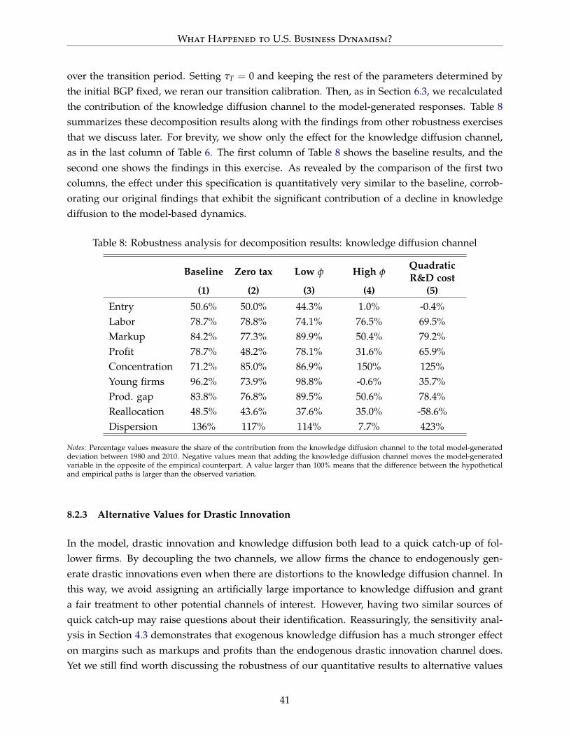
What Happened to U.S. Business Dynamism?
over the transition period. Setting τT = 0 and keeping the rest of the parameters determined bythe initial BGP fixed, we reran our transition calibration. Then, as in Section 6.3, we recalculatedthe contribution of the knowledge diffusion channel to the model-generated responses. Table 8summarizes these decomposition results along with the findings from other robustness exercisesthat we discuss later. For brevity, we show only the effect for the knowledge diffusion channel,as in the last column of Table 6. The first column of Table 8 shows the baseline results, and thesecond one shows the findings in this exercise. As revealed by the comparison of the first twocolumns, the effect under this specification is quantitatively very similar to the baseline, corrob-orating our original findings that exhibit the significant contribution of a decline in knowledgediffusion to the model-based dynamics.
Table 8: Robustness analysis for decomposition results: knowledge diffusion channel
Baseline Zero tax ** Low φ ** * High φ *QuadraticR&D cost
(1) (2) (3) (4) (5)
Entry 50.6% 50.0% 44.3% 1.0% -0.4%Labor 78.7% 78.8% 74.1% 76.5% 69.5%Markup 84.2% 77.3% 89.9% 50.4% 79.2%Profit 78.7% 48.2% 78.1% 31.6% 65.9%Concentration 71.2% 85.0% 86.9% 150% 125%Young firms 96.2% 73.9% 98.8% -0.6% 35.7%Prod. gap 83.8% 76.8% 89.5% 50.6% 78.4%Reallocation 48.5% 43.6% 37.6% 35.0% -58.6%Dispersion 136% 117% 114% 7.7% 423%
Notes: Percentage values measure the share of the contribution from the knowledge diffusion channel to the total model-generateddeviation between 1980 and 2010. Negative values mean that adding the knowledge diffusion channel moves the model-generatedvariable in the opposite of the empirical counterpart. A value larger than 100% means that the difference between the hypotheticaland empirical paths is larger than the observed variation.
8.2.3 Alternative Values for Drastic Innovation
In the model, drastic innovation and knowledge diffusion both lead to a quick catch-up of fol-lower firms. By decoupling the two channels, we allow firms the chance to endogenously gen-erate drastic innovations even when there are distortions to the knowledge diffusion channel. Inthis way, we avoid assigning an artificially large importance to knowledge diffusion and granta fair treatment to other potential channels of interest. However, having two similar sources ofquick catch-up may raise questions about their identification. Reassuringly, the sensitivity anal-ysis in Section 4.3 demonstrates that exogenous knowledge diffusion has a much stronger effecton margins such as markups and profits than the endogenous drastic innovation channel does.Yet we still find worth discussing the robustness of our quantitative results to alternative values
41
What Happened to U.S. Business Dynamism?
of φ. To this end, we recalibrate the transition of the model under the assumption of a low anda high value of φ (keeping other parameters fixed) and regenerate our decomposition results inthese alternative environments.
We start with the discussion of low-φ case. Setting φ to one-tenth of the original valuewhile keeping other parameters listed in Table 1 fixed, we recalibrate the parameters that definethe transition path of the model. Next, we recompute the quantitative effect of the recalibrateddecline in knowledge diffusion intensity. The results, shown in the third column of Table 8,demonstrate that the original findings still go through: The knowledge diffusion channel has avery high power in explaining the transition path of the model variables.
Next, we repeat the same exercise with a high value of φ, which we set to about 42 per-cent, 10 times the baseline value. This extreme value implies that almost half of the innovationsgenerated by followers are of a drastic nature and leaves very little scope for the exogenousknowledge diffusion in the model. The fourth column of Table 8 presents the results based onthe recalibrated transition path in this specification. The significant finding is that in this case,the knowledge diffusion channel contributes very little to variations in entry-related margins (inparticular, the entry rate and the employment share of young firms). These margins are nowalmost fully explained by a calibrated increase in the entry cost (not shown). This finding isperhaps expected given the extremely limited scope for the diffusion channel in this specifica-tion. But a more striking observation is that even in this constrained specification, the knowledgediffusion channel has the most significant power in driving the increase in market concentration,markups, and aggregate profit share and the reciprocal decline in aggregate labor share. Thecommon denominator of these margins is that they crucially depend on the shifts in the distribu-tion of sectors across technology gaps. Therefore, this exercise shows that even in this case, thechanges in knowledge diffusion are the main driver of such distributional shifts in the economy.
8.2.4 R&D Elasticity
In quantitative Schumpeterian growth literature, a commonly used value for the labor elasticityof R&D expenditure is 0.5, implying a quadratic R&D cost function (see Acemoglu et al., 2018,for a discussion). Therefore, we next repeat our decomposition exercise under the assumption ofquadratic R&D cost functions. To this end, we recalibrate the transition path, setting γ = γ = 2while keeping other calibrated parameters listed in Table 1 fixed. The last column in Table 8presents the results. Similar to the exercise with a higher drastic innovation probability, weobserve that while the explanatory power of a decline in knowledge diffusion becomes negligible(most of the entry decline is driven by higher entry cost), the channel retains its significance inaccounting for changes in variables such as aggregate profit share and average markup.
A seemingly confusing finding is that a decline in knowledge diffusion plays a considerablerole in driving the decline in young firms’ employment share despite its negligible effect on firm
42
What Happened to U.S. Business Dynamism?
entry. The reason is that, in fact, the decline in knowledge diffusion does not fail to generatemeaningful action in firm entry (as opposed to the exercise with a high φ). While lower δ
provides an additional force that drives down firm entry, it also causes an initial jump in thisvariable, implying a steeper decline over the transition.28 Therefore, shutting down the diffusionchannel implies a smaller magnitude for the decline in firm entry; but because the initial jump isalso removed, the terminal value of firm entry barely changes. Therefore, we obtain a seeminglynegligible contribution from the knowledge diffusion channel, as shown in Table 8 (see alsoequation 30). Nevertheless, the ability of this channel to generate meaningful dynamics stillmanifests itself in other variables such as the employment share of young firms.
8.3 Model Extensions
In this study, we focus on 10 empirical regularities and aim at analyzing them in a comprehensivebut parsimonious setting. Yet the model is flexible enough to incorporate other features that canprove useful in future research. One such extension could be the generalization of the marketstructure in intermediate-good production. Currently, perfect competition among intermediate-good producers implies that only one firm produces the particular good. As a result, the concen-tration measure (HHI) takes two values (1/2 or 1). A straightforward generalization would be touse a constant-elasticity-of-substitution production function at the industry level à la Aghion etal. (2001), which would make both firms produce in each product line. Accordingly, one wouldobtain more heterogeneity in terms of concentration. However, this extension would complicatethe computation of the model, especially over the transition (a key contribution of the study),without adding much further insight, as the key mechanism of the model would remain intact.Therefore, we stuck to the current version of the model.
Another possible extension relates to the labor share distribution of firms. Autor et al. (2017b)and Kehrig and Vincent (2018) argue that most of the labor share decline at the industry levelstems from the relocation of activity to low-labor-share, highly productive firms (rather than awidespread decline in firms’ labor share). Accordingly, they find that the labor share distributionof firms has barely changed.29 On the one hand, our model is consistent with the empiricalobservation that low-labor-share firms capture a higher share of economic activity as marketconcentration increases. On the other hand, the model does not generate a stable labor sharedistribution.30 To reflect on these empirical findings, the model can be extended by assigningheterogeneous research productivity types to firms.31 In this study, we did not take that route,because it would come at a significant loss in tractability—an essential feature for our structural
28 This initial response stems from the increase in leader’s value, incentivizing firm entry, especially to leveledsectors. As the elasticity of R&D cost function is lower in this exercise, the initial response of firm entry to the changein incumbent firms’ value is also more pronounced.
29 The evidence is more decisive for the manufacturing sector.30 Indeed, the distribution shifts toward lower-labor-share firms in lockstep with increasing concentration and
average markups in the model.31Aghion et al. (2019) consider such type heterogeneity to analyze labor share dynamics of incumbent firms.
43
What Happened to U.S. Business Dynamism?
analysis of transitional dynamics. While the aforementioned regularities are a few from manyother empirical trends that could be added to the extensive set analyzed here, notice that they arenot crucial for our main quantitative results (the pecking order among potential drivers in termsof their power in explaining observed trends in the economy). This corollary holds because theinconsistency is not specific to the dynamics created by a particular channel, but it is rather amodel feature. Therefore, we proceed with the current parsimonious framework and leave theseadditional considerations to future research.
9 New Evidence for Future Research: U.S. Patent Trends
In Section 6, we established that a decline in knowledge diffusion is the dominant culprit behindthe observed market power and business dynamism trends in the United States. A natural follow-up question is, what caused a decline in knowledge diffusion? Providing a decisive answer tothis question is beyond the scope of the analysis presented here. Nevertheless, we think it isworth reflecting briefly on this question in light of some new empirical evidence, which mayprove useful in guiding future research in this direction.
In Akcigit and Ates (2019), we elaborate on several candidates that could justify a decline inknowledge diffusion—use of tacit knowledge and data in production, outsourcing of productionprocesses, and regulations, to name a few. We extend the discussion here by providing newevidence on the use (or abuse) of patents in the United States. Patent and reassignment data fromthe U.S. Patent and Trademark Office (USPTO) provide a fertile ground for investigating patternsof knowledge diffusion, as firms rely heavily on patent protection to shield themselves fromimitators. A decline in imitators’ ability to copy and learn from market leaders’ technology due toheavier, and especially strategic, use of patents by the leaders would limit the flow of knowledgebetween firms and lead to a reduction in the intensity of knowledge diffusion. Therefore, wenow turn our attention to the changes in the use of patents in the U.S. economy across time.
Patent Concentration and Post-1980 Trends
As we reviewed in Section 2, many indicators of business dynamism suggest a declining trendsince the 1980s along with rising market concentration. We first investigate if there has beena concomitant change in patenting concentration. To answer this question, Figure 9a looks atthe share of patents registered by the top 1 percent of innovating firms with the largest patentstocks. The ratio exhibits a dramatic increase. While in the early 1980s about 35 percent ofpatents were registered by the top 1 percent of firms sitting on the largest patent stocks, this ratioreached almost 50 percent in three decades.32 In addition, the share of patents registered by newentrants (firms that patent for the first time) exhibits the opposite trend: Notwithstanding the
32Notice that the increase in this ratio has been larger than the rise in market concentration (see Autor et al., 2017b).
44
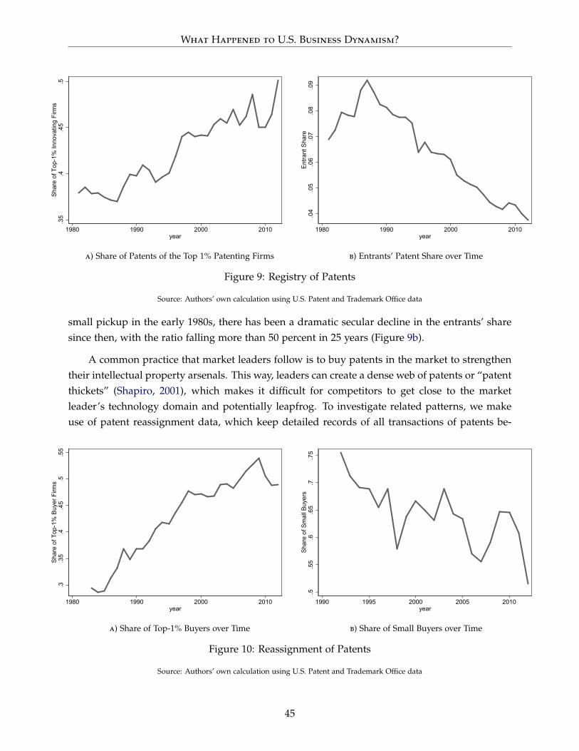
What Happened to U.S. Business Dynamism?
.35
.4.4
5.5
Shar
e of
Top
-1%
Inno
vatin
g Fi
rms
1980 1990 2000 2010year
a) Share of Patents of the Top 1% Patenting Firms
.04
.05
.06
.07
.08
.09
Entra
nt S
hare
1980 1990 2000 2010year
b) Entrants’ Patent Share over Time
Figure 9: Registry of Patents
Source: Authors’ own calculation using U.S. Patent and Trademark Office data
small pickup in the early 1980s, there has been a dramatic secular decline in the entrants’ sharesince then, with the ratio falling more than 50 percent in 25 years (Figure 9b).
A common practice that market leaders follow is to buy patents in the market to strengthentheir intellectual property arsenals. This way, leaders can create a dense web of patents or “patentthickets” (Shapiro, 2001), which makes it difficult for competitors to get close to the marketleader’s technology domain and potentially leapfrog. To investigate related patterns, we makeuse of patent reassignment data, which keep detailed records of all transactions of patents be-
.3.3
5.4
.45
.5.5
5Sh
are
of T
op-1
% B
uyer
Firm
s
1980 1990 2000 2010year
a) Share of Top-1% Buyers over Time
.5.5
5.6
.65
.7.7
5Sh
are
of S
mal
l Buy
ers
1990 1995 2000 2005 2010year
b) Share of Small Buyers over Time
Figure 10: Reassignment of Patents
Source: Authors’ own calculation using U.S. Patent and Trademark Office data
45
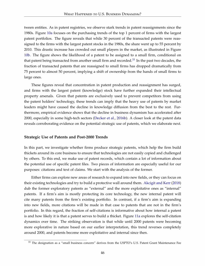
What Happened to U.S. Business Dynamism?
tween entities. As in patent registries, we observe stark trends in patent reassignments since the1980s. Figure 10a focuses on the purchasing trends of the top 1 percent of firms with the largestpatent portfolios. The figure reveals that while 30 percent of the transacted patents were reas-signed to the firms with the largest patent stocks in the 1980s, the share went up to 55 percent by2010. This drastic increase has crowded out small players in the market, as illustrated in Figure10b. The figure shows the likelihood of a patent to be assigned to a small firm, conditional onthat patent being transacted from another small firm and recorded.33 In the past two decades, thefraction of transacted patents that are reassigned to small firms has dropped dramatically from75 percent to almost 50 percent, implying a shift of ownership from the hands of small firms tolarge ones.
These figures reveal that concentration in patent production and reassignment has surged,and firms with the largest patent (knowledge) stock have further expanded their intellectualproperty arsenals. Given that patents are exclusively used to prevent competitors from usingthe patent holders’ technology, these trends can imply that the heavy use of patents by marketleaders might have caused the decline in knowledge diffusion from the best to the rest. Fur-thermore, empirical evidence shows that the decline in business dynamism has accelerated after2000, especially in some high-tech sectors (Decker et al., 2016b). A closer look at the patent datareveals corroborating evidence on the potential strategic use of patents, which we elaborate next.
Strategic Use of Patents and Post-2000 Trends
In this part, we investigate whether firms produce strategic patents, which help the firm buildthickets around its core business to ensure that technologies are not easily copied and challengedby others. To this end, we make use of patent records, which contain a lot of information aboutthe potential use of specific patent files. Two pieces of information are especially useful for ourpurposes: citations and text of claims. We start with the analysis of the former.
Either firms can explore new areas of research to expand into new fields, or they can focus ontheir existing technologies and try to build a protective wall around them. Akcigit and Kerr (2018)dub the former exploratory patents as “external” and the more exploitative ones as “internal”patents. If a firm’s aim is mostly protecting its core technology, the new internal patent willcite many patents from the firm’s existing portfolio. In contrast, if a firm’s aim is expandinginto new fields, more citations will be made in that case to patents that are not in the firm’sportfolio. In this regard, the fraction of self-citations is informative about how internal a patentis and how likely it is that a patent serves to build a thicket. Figure 11a explores the self-citationdynamics over time. The striking observation is that while until 2000 patents were becomingmore explorative in nature based on our earlier interpretation, this trend reverses completelyaround 2000, and patents become more exploitative and internal since then.
33 The designation as a “small business concern” derives from the USPTO’s U.S. Patent Grant Maintenance Fee
46
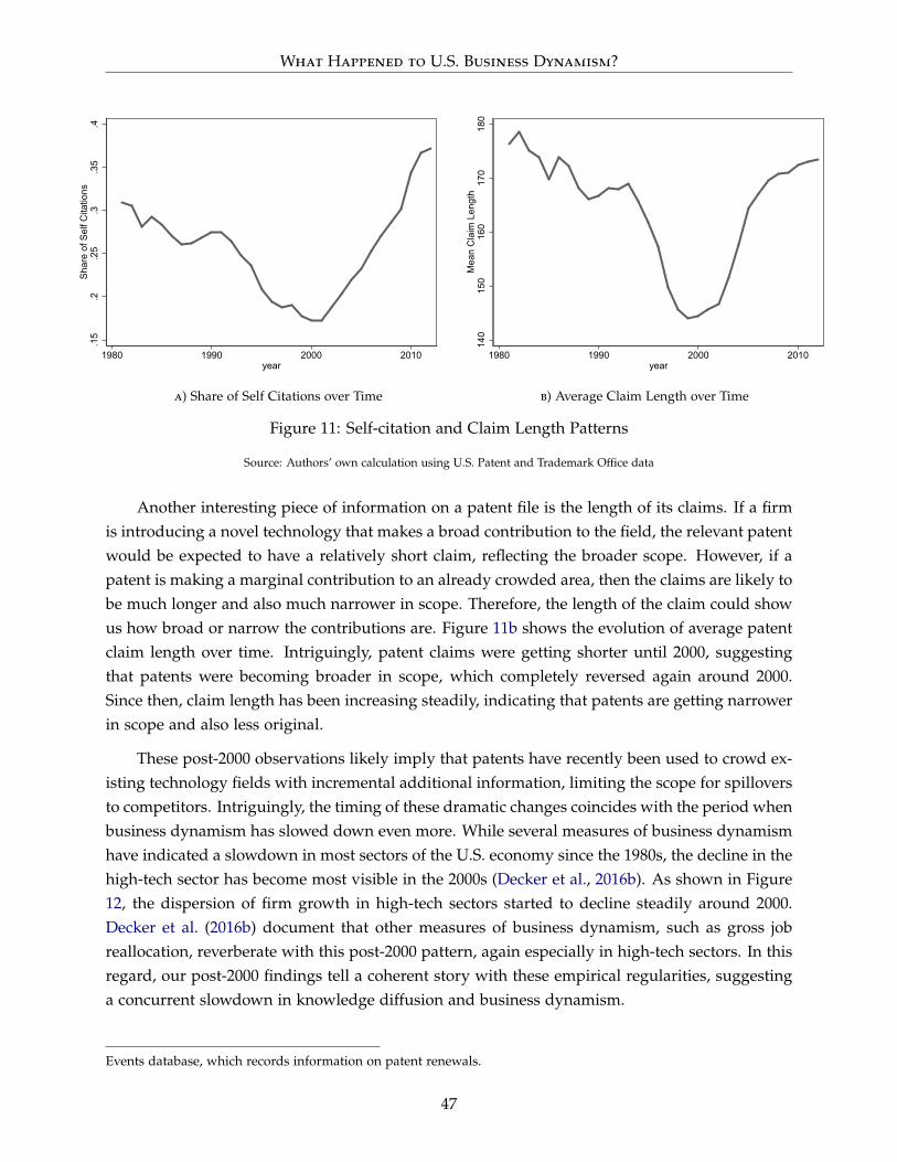
What Happened to U.S. Business Dynamism?
.15
.2.2
5.3
.35
.4Sh
are
of S
elf C
itatio
ns
1980 1990 2000 2010year
a) Share of Self Citations over Time
140
150
160
170
180
Mea
n C
laim
Len
gth
1980 1990 2000 2010year
b) Average Claim Length over Time
Figure 11: Self-citation and Claim Length Patterns
Source: Authors’ own calculation using U.S. Patent and Trademark Office data
Another interesting piece of information on a patent file is the length of its claims. If a firmis introducing a novel technology that makes a broad contribution to the field, the relevant patentwould be expected to have a relatively short claim, reflecting the broader scope. However, if apatent is making a marginal contribution to an already crowded area, then the claims are likely tobe much longer and also much narrower in scope. Therefore, the length of the claim could showus how broad or narrow the contributions are. Figure 11b shows the evolution of average patentclaim length over time. Intriguingly, patent claims were getting shorter until 2000, suggestingthat patents were becoming broader in scope, which completely reversed again around 2000.Since then, claim length has been increasing steadily, indicating that patents are getting narrowerin scope and also less original.
These post-2000 observations likely imply that patents have recently been used to crowd ex-isting technology fields with incremental additional information, limiting the scope for spilloversto competitors. Intriguingly, the timing of these dramatic changes coincides with the period whenbusiness dynamism has slowed down even more. While several measures of business dynamismhave indicated a slowdown in most sectors of the U.S. economy since the 1980s, the decline in thehigh-tech sector has become most visible in the 2000s (Decker et al., 2016b). As shown in Figure12, the dispersion of firm growth in high-tech sectors started to decline steadily around 2000.Decker et al. (2016b) document that other measures of business dynamism, such as gross jobreallocation, reverberate with this post-2000 pattern, again especially in high-tech sectors. In thisregard, our post-2000 findings tell a coherent story with these empirical regularities, suggestinga concurrent slowdown in knowledge diffusion and business dynamism.
Events database, which records information on patent renewals.
47
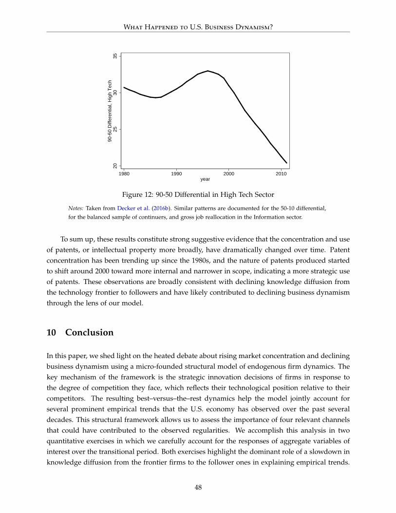
What Happened to U.S. Business Dynamism?
2025
3035
90−5
0 D
iffer
entia
l, H
igh
Tech
1980 1990 2000 2010year
Figure 12: 90-50 Differential in High Tech Sector
Notes: Taken from Decker et al. (2016b). Similar patterns are documented for the 50-10 differential,for the balanced sample of continuers, and gross job reallocation in the Information sector.
To sum up, these results constitute strong suggestive evidence that the concentration and useof patents, or intellectual property more broadly, have dramatically changed over time. Patentconcentration has been trending up since the 1980s, and the nature of patents produced startedto shift around 2000 toward more internal and narrower in scope, indicating a more strategic useof patents. These observations are broadly consistent with declining knowledge diffusion fromthe technology frontier to followers and have likely contributed to declining business dynamismthrough the lens of our model.
10 Conclusion
In this paper, we shed light on the heated debate about rising market concentration and decliningbusiness dynamism using a micro-founded structural model of endogenous firm dynamics. Thekey mechanism of the framework is the strategic innovation decisions of firms in response tothe degree of competition they face, which reflects their technological position relative to theircompetitors. The resulting best–versus–the–rest dynamics help the model jointly account forseveral prominent empirical trends that the U.S. economy has observed over the past severaldecades. This structural framework allows us to assess the importance of four relevant channelsthat could have contributed to the observed regularities. We accomplish this analysis in twoquantitative exercises in which we carefully account for the responses of aggregate variables ofinterest over the transitional period. Both exercises highlight the dominant role of a slowdown inknowledge diffusion from the frontier firms to the follower ones in explaining empirical trends.
48
What Happened to U.S. Business Dynamism?
This result hinges on the trickle-down effect of slower knowledge diffusion on firm entry as wellas the compositional dynamics arising from the less frequent catching–up of followers with themarket leaders, distorting competition dynamics.
In their extensive study, Andrews et al. (2016) show a widening productivity gap betweenfrontier and laggard firms, which the authors interpret to indicate declining knowledge diffusion.In parallel, our complementary empirical investigation presents new evidence on the potentialsymptoms of slower knowledge diffusion from the U.S. patent data. In particular, we docu-ment a higher concentration of patent ownership through both production and acquisition ofnew patents, echoing the broader patterns of market concentration. Moreover, we observe anincreasingly more strategic use of patents in the post-2000 era, as indicated by their increasinglyinternal nature. These changes have likely contributed to the decline in business dynamism, withthe flow of knowledge or spillovers to competitors becoming more constrained over time.
The findings of this paper also present a direction for both future research and policy design.As discussed previously, several channels could have distorted the diffusion of knowledge. Ashort list of candidates include globalization, regulations, the changing nature of production andthe increasing use of data. In addition, our empirical investigation points to an intensified useof patents to deter knowledge spillovers and potential competition. Opening the black box ofthe nature of knowledge diffusion and determining the drivers of its slowdown are vital topicsfor future research in this direction. In terms of policy, the results suggest that the appropri-ate response to revive business dynamism should focus on post-entry distortions that impedecompetition between leader and follower firms. Such competition policy would not only affectincumbent firms, but also incentivize business entry through positive trickle-down effects.
Finally, our work emphasizes the importance of a comprehensive approach that links micro-level changes in market primitives to macro outcomes in analyzing the drivers of prominentempirical trends in the U.S. economy. The distinction between market primitives and the ob-served outcomes is essential in that it helps us avoid enforcing a certain relationship betweenmacro outcomes that might be related in various ways—a criticism by Syverson (2019)—and getto the root of those outcomes. While each one of candidate mechanisms can potentially speakto some specific trends, a comparative study of all these channels in light of all empirical reg-ularities allows us to determine the relative quantitative bite of these channels and to identifythe potential common cause. We believe that such quantitative comparison is vital for academicwork to guide policy decisions.
49
What Happened to U.S. Business Dynamism?
References
Acemoglu, Daron and Pascual Restrepo, “Robots and Jobs: Evidence from US Labor Markets,”2017. National Bureau of Economic Research Working Paper 23285.
and Ufuk Akcigit, “Intellectual Property Rights Policy, Competition and Innovation,” Journalof the European Economic Association, 2012, 10 (1), 1–42.
, , Douglas Hanley, and William Kerr, “Transition to Clean Technology,” Journal of PoliticalEconomy, 2016, 124 (1), 52–104.
, , Harun Alp, Nicholas Bloom, and William Kerr, “Innovation, Reallocation, and Growth,”American Economic Review, 2018, 108 (11), 3450–3491.
Aghion, Philippe, Antonin Bergeaud, Timo Boppart, Peter J. Klenow, and Huiyu Li, “A Theoryof Falling Growth and Rising Rents,” 2019. mimeo.
, Christopher Harris, and John Vickers, “Competition and Growth with Step-by-step Innova-tion: An Example,” European Economic Review, 1997, 41 (3-5), 771–782.
, , Peter Howitt, and John Vickers, “Competition, Imitation and Growth with Step-by-StepInnovation,” Review of Economic Studies, 2001, 68 (3), 467–492.
, Nick Bloom, Richard Blundell, Rachel Griffith, and Peter Howitt, “Competition and Inno-vation: An Inverted-U Relationship,” Quarterly Journal of Economics, 2005, 120 (2), 701–728.
Akcigit, Ufuk and Sina T. Ates, “Ten Facts on Declining Business Dynamism and Lessons fromEndogenous Growth Theory,” 2019. University of Chicago mimeo.
and William R. Kerr, “Growth through Heterogeneous Innovations,” Journal of Political Econ-omy, 2018, 126 (4), 1374–1443.
, Sina T. Ates, and Giammario Impullitti, “Innovation and Trade Policy in a GlobalizedWorld,” 2018. National Bureau of Economic Research Working Paper 24543.
Andrews, Dan, Chiara Criscuolo, and Peter N. Gal, “Frontier Firms, Technology Diffusion andPublic Policy,” 2015. OECD Productivity Working Paper No. 2.
, , and , “The Best versus the Rest: The Global Productivity Slowdown, Divergence acrossFirms and the Role of Public Policy,” 2016. OECD Productivity Working Paper 5/2016.
Appelbaum, Binyamin, “Corporate Tax Code Proves Hard to Change,” The New York Times, 2011.https://www.nytimes.com/2011/01/28/us/politics/28tax.html?_r=1, accessed on 1/28/2019.
Autor, David, David Dorn, Lawrence F. Katz, Christina Patterson, and John Van Reenen, “Con-centrating on the Fall of the Labor Share,” American Economic Review, 2017, 107 (5), 180–85.
, , , , and , “The Fall of the Labor Share and the Rise of Superstar Firms,” 2017.National Bureau of Economic Research Working Paper 23396.
Azar, José, Ioana Marinescu, and Marshall I. Steinbaum, “Labor Market Concentration,” 2017.National Bureau of Economic Research Working Paper 24147.
Bajgar, Matej, Giuseppe Berlingieri, Sara Calligaris, Chiara Criscuolo, and Jonathan Timmis,“Industry Concentration in Europe and North America,” 2019. OECD Productivity WorkingPapers No. 18.
50
What Happened to U.S. Business Dynamism?
Baker, Jonathan B., “Economics and Politics: Perspectives on the Goals and Future of Antitrust,”Fordham Law Review, 2012, 81, 2175.
Barkai, Simcha, “Declining Labor and Capital Shares,” 2017. mimeo.
Bessen, James E., “Accounting for Rising Corporate Profits: Intangibles or Regulatory Rents?,”2016. Law & Economics Paper Series 16-18, Boston University School of Law.
, “Information Technology and Industry Concentration,” 2017. Law & Economics Paper Series17–41, Boston University School of Law.
Bivens, Josh, Elise Gould, Lawrence Mishel, and Heidi Shierholz, “Raising America’s Pay:Why It’s Our Central Economic Policy Challenge,” 2014. Economic Policy Institute. Washing-ton, D.C.
, Lora Engdahl, Elise Gould, Teresa Kroeger, Celine McNicholas, Lawrence Mishel, ZaneMokhiber, Heidi Shierholz, Marni von Wilpert, Valerie Wilson, and Ben Zipperer, “HowTodayŠs Unions Help Working People: Giving Workers the Power to Improve Their Jobs andUnrig the Economy,” 2017. Economic Policy Institute. Washington, D.C.
Bloom, Nicholas, Charles I. Jones, John Van Reenen, and Michael Webb, “Are Ideas GettingHarder to Find?,” 2017. National Bureau Economic Research Working Paper 23782.
Boehm, Christoph E., Aaron Flaaen, and Nitya Pandalai-Nayar, “Multinationals Offshoring, andthe Decline of U.S. Manufacturing,” 2017. Center for Economic Studies, U.S. Census Bureau,Working Papers 17-22.
Bravo-Biosca, Albert, Chiara Criscuolo, and Carlo Menon, “What Drives the Dynamics of Busi-ness Growth?,” 2013. OECD Science, Technology and Industry Policy Papers No. 1.
Budd, Christopher, Christopher Harris, and John Vickers, “A Model of the Evolution ofDuopoly: Does the Asymmetry between Firms Tend to Increase or Decrease?,” Review of Eco-nomic Studies, 1993, 60 (3), 543–573.
Calligaris, Sara, Chiara Criscuolo, and Luca Marcolin, “Mark-ups in the Digital Era,” 2018.OECD Working Paper 2018-10.
Congressional Budget Office, “Federal Support for Research and Development,” 2007. Wash-ington, D.C. https://www.cbo.gov/publication/18750.
, “International Comparisons of Corporate Income Tax Rates,” 2017. Washington, D.C.https://www.cbo.gov/publication/52419.
Cooley, Thomas F. and Edward C. Prescott, “Economic Growth and Business Cycles,” inThomas F Cooley, ed., Frontiers of Business Cycle Research, Princeton University Press, 1995,pp. 1–38.
Crain, Nicole V. and W. Mark Crain, “The Impact of Regulatory Costs on Small Firms,”2010. Washington, D.C.: Office of Advocacy, U.S. Small Business Administrationhttps://www.sba.gov/advocacy/impact-regulatory-costs-small-firms.
Crouzet, Nicolas and Janice Eberly, “Understanding Weak Capital Investment: The Role ofMarket Concentration and Intangibles,” 2018. Jackson Hole Economic Policy Symposium.
Cunningham, Colleen, Song Ma, and Florian Ederer, “Killer Acquisitions,” Academy of Manage-ment Proceedings, 2018, (1).
51
What Happened to U.S. Business Dynamism?
Davis, Steven J. and John C. Haltiwanger, “Dynamism Diminished: The Role of Housing Mar-kets and Credit Conditions,” 2019. National Bureau of Economic Research Working Paper25466.
Davis, Steven, John Haltiwanger, and Scott Schuh, Job Creation and Destruction, Cambridge, MA:MIT Press, 1996.
De Loecker, Jan and Jan Eeckhout, “The Rise of Market Power and The Macroeconomic Impli-cations,” 2017. National Bureau of Economic Research Working Paper 23687.
and , “Global Market Power,” 2018. National Bureau of Economic Research Working Paper24768.
De Ridder, Maarten, “Market Power and Innovation in the Intangible Economy,” 2019.Cambridge-INET Working Paper 2019/08.
Decker, Ryan A., John C. Haltiwanger, Ron S. Jarmin, and Javier Miranda, “Changing BusinessDynamism and Productivity: Shocks vs. Responsiveness,” 2018. National Bureau EconomicResearch Working Paper 24236.
, John Haltiwanger, Ron S. Jarmin, and Javier Miranda, “Where Has All The Skewness Gone?The Decline In High-Growth (Young) Firms In The US,” 2015. National Bureau of EconomicResearch Working Paper 21776.
, , , and , “Declining Business Dynamism: What We Know and the Way Forward,”American Economic Review: Papers & Proceedings, 2016, 106 (5), 203–07.
, , , and , “Where Has All The Skewness Gone? The Decline in High-Growth (Young)Firms in The US,” European Economic Review, 2016, 86, 4–23.
Decker, Ryan, John Haltiwanger, Ron Jarmin, and Javier Miranda, “The Role of Entrepreneur-ship in US Job Creation and Economic Dynamism,” Journal of Economic Perspectives, 2014, 28(3), 3–24.
Diez, Federico, Daniel Leigh, and Suchanan Tambunlertchai, “Global Market Power and ItsMacroeconomic Implications,” 2018. International Monetary Fund Working Papers 18/137.
Eggertsson, Gauti B., Jacob A. Robbins, and Ella Getz Wold, “Kaldor and Piketty’s Facts: TheRise of Monopoly Power in the United States,” 2018. National Bureau of Economic ResearchWorking Paper 24287.
Elsby, Michael, Bart Hobijn, and Aysegul Sahin, “The Decline of the U.S. Labor Share,” 2013.Federal Reserve Bank of San Francisco, Working Paper 2013-27.
Farber, Henry S., Daniel Herbst, Ilyana Kuziemko, and Suresh Naidu, “Unions and InequalityOver the Twentieth Century: New Evidence from Survey Data,” 2018. National Bureau ofEconomic Research Working Paper 24587.
Farhi, Emmanuel and François Gourio, “Accounting for Macro-Finance Trends: Market Power,Intangibles, and Risk Premia,” 2018. National Bureau of Economic Research Working Paper25282.
Fernald, John G., “A Quarterly, Utilization-Adjusted Series on Total Factor Productivity,” 2012.Federal Reserve Bank of San Francisco, Working Paper Series 2012–19.
52
What Happened to U.S. Business Dynamism?
Furman, Jason and Laura Giuliano, “New Data Show That RoughlyOne-Quarter of U.S. Workers Hold an Occupational License,” 2016.https://obamawhitehouse.archives.gov/blog/2016/06/17/new-data-show-roughly-one-quarter-us-workers-hold-occupational-license.
and Peter Orszag, “Slower Productivity and Higher Inequality: Are They Related?,” 2018.Working Paper 2018-4, Peterson Institute for International Economics.
Gordon, Robert J., The Rise and Fall of American Growth: The U.S. Standard of Living since the CivilWar, Princeton University Press, 2016.
Gourio, François, Todd Messer, and Michael Siemer, “What Is the Economic Impact of theSlowdown in New Business Formation?,” Chicago Fed Letter, 2014, (Sep).
Gravelle, Jane, “Historical Effective Marginal Tax Rates on Capital Income,” 2004. CongressionalResearch Service RS21706, Library of Congress.
Grossman, Gene M., Elhanan Helpman, Ezra Oberfield, and Thomas Sampson, “The Produc-tivity Slowdown and the Declining Labor Share: A Neoclassical Exploration,” 2017. NationalBureau of Economic Research Working Paper 23853.
Grullon, Gustavo, Yelena Larkin, and Roni Michaely, “Are U.S. Industries Becoming MoreConcentrated?,” 2017. mimeo.
Gutiérrez, Germán and Thomas Philippon, “Investment-less Growth: An Empirical Investiga-tion,” 2016. National Bureau of Economic Research Working Paper 22897.
and , “Declining Competition and Investment in the U.S.,” 2017. National Bureau of Eco-nomic Research Working Paper 23583.
and , “Fading Stars,” 2019. National Bureau of Economic Research Working Paper 25529.
, Callum Jones, and Thomas Philippon, “Entry Costs and the Macroeconomy,” 2019. NationalBureau of Economic Research Working Paper 25609.
Hall, Robert E., “New Evidence on Market Power, Profit, Concentration, and the Role of Mega-Firms in the U.S. Economy,” 2018. Standofrd University, mimeo.
Haltiwanger, John, Ron S. Jarmin, and Javier Miranda, “Who Creates Jobs? Small versus Largeversus Young,” The Review of Economics and Statistics, 2013, 95 (2), 347–361.
Harris, Christopher and John Vickers, “Perfect Equilibrium in a Model of a Race,” Review ofEconomic Studies, 1985, 52 (2), 193–209.
and , “Racing with Uncertainty,” Review of Economic Studies, 1987, 54 (1), 1–21.
Hopenhayn, Hugo, Julian Neira, and Rish Singhania, “From Population Growth to Firm De-mographics: Implications for Concentration, Entrepreneurship and the Labor Share,” 2018.National Bureau of Economic Research Working Paper 25382.
Kalemli-Ozcan, Sebnem, Bent Sorensen, Carolina Villegas-Sanchez, and Vadym Volosovych,“How to Construct Nationally Representative Firm Level Data from ORBIS Global Databaseand What Do We Learn from Representativeness?,” 2019. mimeo.
Karabarbounis, Loukas and Brent Neiman, “The Global Decline of the Labor Share,” QuarterlyJournal of Economics, 2013, 129 (1), 61–103.
53
What Happened to U.S. Business Dynamism?
Karahan, Fatih, Benjamin Pugsley, and Aysegul Sahin, “Demographic Origins of the StartupDeficit,” 2016. New York Fed, mimeo.
Kaymak, Baris and Immo Schott, “Corporate Tax Cuts and the Decline of the Labor Share,”2018. Society for Economic Dynamics, 2018 Meeting Papers 943.
Kehrig, Matthias and Nicolas Vincent, “The Micro-Level Anatomy of the Labor Share Decline,”2018. National Bureau of Economic Research Working Paper 25275.
Khan, Lina M., “Amazon’s Antitrust Paradox,” Yale Law Journal, 2016, 126, 710–805.
Klapper, Leora and Inessa Love, “The Impact of Business Environment Reforms on New FirmRegistration,” 2010. World Bank Impact Evaluation series no. IE 49, Policy Research workingpaper no. WPS 5493.
, Luc Laeven, and Raghuram Rajan, “Entry Regulation as a Barrier to Entrepreneurship,”Journal of Financial Economics, 2006, 82 (3), 591–629.
Klette, Tor Jakob and Samuel Kortum, “Innovating Firms and Aggregate Innovation,” Journal ofPolitical Economy, 2004, 112 (5), 986–1018.
Kocieniewski, David, “G.E.’s Strategies Let It Avoid Taxes Altogether,” The New York Times, 2011.https://www.nytimes.com/2011/03/25/business/economy/25tax.html?pagewanted=all, ac-cessed on 1/28/2019.
Kortum, Samuel, “Equilibrium R&D and the Patent–R&D Ratio: U.S. Evidence,” The AmericanEconomic Review, 1993, 83 (2), 450–457.
Laubach, Thomas and John C. Williams, “Measuring the Natural Rate of Interest,” Review ofEconomics and Statistics, 2003, 85 (4), 1063–1070.
Lawrence, Robert Z., “Recent Declines in Labor’s Share in U.S. Income: A Preliminary Neoclas-sical Account,” 2015. National Bureau of Economic Research Working Paper 21296.
Liu, Ernest, Atif Mian, and Amir Sufi, “Low Interest Rates, Market Power, and ProductivityGrowth,” 2019. Becker Friedman Institute Working Papers Series 2019-09.
Lynn, Barry C., Cornered: The New Monopoly Capitalism and The Economics of Destruction, JohnWiley & Sons Hoboken, NJ, 2010.
Naidu, Suresh, Eric A. Posner, and Glen Weyl, “Antitrust Remedies for Labor Market Power,”Harv. L. Rev., 2018, 132, 536.
Nekarda, Christopher J. and Valerie A. Ramey, “The Cyclical Behavior of the Price-CostMarkup,” 2013. National Bureau of Economic Research Working Paper 19099.
OECD, “Market Concentration - Note by the BIAC,” 2018. Hearing on Market Concentration.
, “Market Concentration - Note by the United States,” 2018. Hearing on Market Concentration.
Pugsley, Benjamin W., Peter Sedlácek, and Vincent Sterk, “The Nature of Firm Growth,” 2018.Center for Economic Studies, U.S. Census Bureau, Working Paper 18-30.
Rossi-Hansberg, Esteban, Pierre-Daniel Sarte, and Nicholas Trachter, “Diverging Trends inNational and Local Concentration,” 2018. National Bureau of Economic Research WorkingPaper 25066.
54
What Happened to U.S. Business Dynamism?
Shapiro, Carl, “Navigating the Patent Thicket: Cross Licenses, Patent Pools, and Standard Set-ting,” in “Innovation Policy and the Economy, Volume 1” NBER Chapters, National Bureau ofEconomic Research, Inc., October 2001, pp. 119–150.
Summers, Laurence H., “Reflections on the SNew Secular Stagnation HypothesisŠ,” in RichardBaldwin and Coen Teulings, eds., Secular Stagnation: Facts, Causes and Cures, CEPR Press Lon-don, A VoxEU.org eBook, 2014, pp. 27–38.
Summers, Lawrence H., “US Economic Prospects: Secular Stagnation, Hysteresis, and the ZeroLower Bound,” Business Economics, 2014, 49 (2), 65–73.
Syverson, Chad, “Market Structure and Productivity: A Concrete Example,” Journal of PoliticalEconomy, 2004, 112 (6), 1181–1222.
, “Product Substitutability and Productivity Dispersion,” The Review of Economics and Statistics,2004, 86 (2), 534–550.
, “Macroeconomics and Market Power: Facts, Potential Explanations, and OpenQuestions,” Brookings Institution Report, January 2019. Accessed January 21, 2019.https://www.brookings.edu/research/macroeconomics-and-market-power-facts-potential-explanations-and-open-questions/.
The Economist, “Regulating the Internet Giants: The World’s Most Valuable Resource Is NoLonger Oil, but Data,” May 2017.
Tyson, Laura and Greg Linden, “The Corporate R&D Tax Credit and US Innovation and Com-petitiveness: Gauging the Economic and Fiscal Effectiveness of the Credit,” 2012. Washington:Center for American Progress.
U.S. Bureau of Economic Analysis, “Corporate Profits after Tax (without IVA and CCAdj) [CP]and Federal Government: Tax Receipts on Corporate Income [FCTAX],” 2019. retrieved fromFRED, Federal Reserve Bank of St. Louis; https://fred.stlouisfed.org/graph/?g=aWA accessedon 1/26/2019.
U.S. Chamber of Commerce Foundation, “The Regulatory Impact on Small Businesses: Com-plex. Cumbersome. Costly.,” 2017. Washington, D.C.
Williams, John C., “The Decline in the Natural Rate of Interest,” Business Economics, 2015, 50 (2),57–60.
55
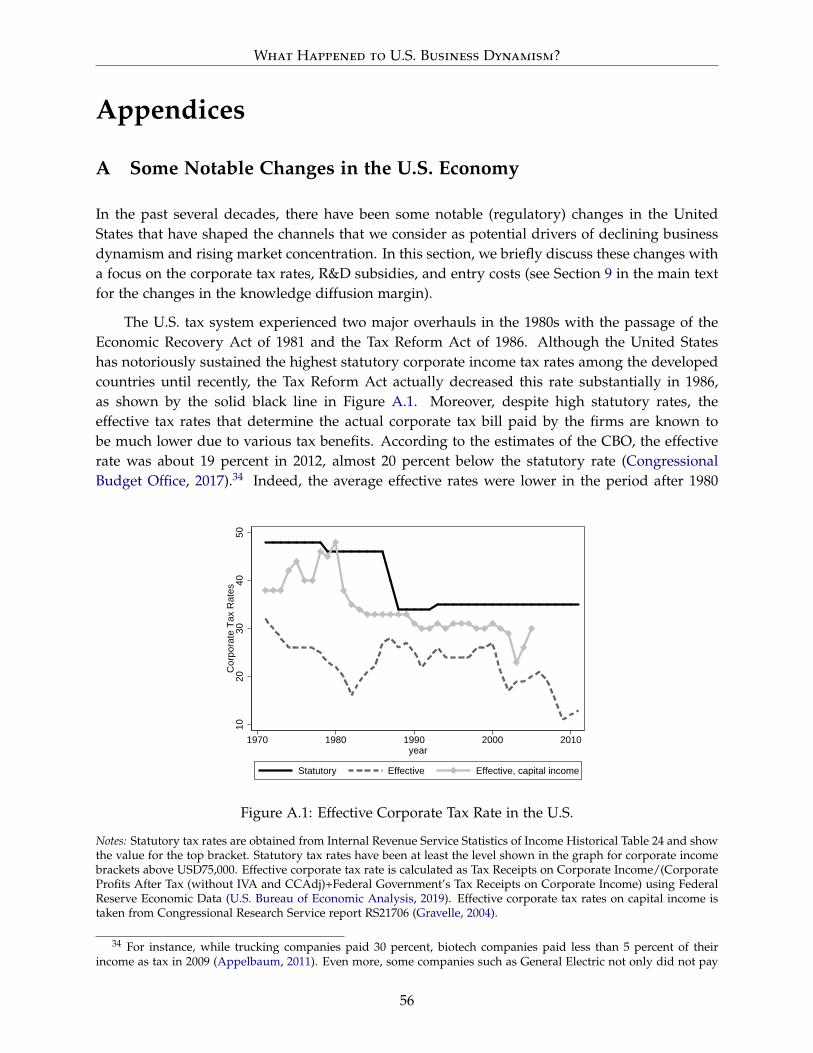
What Happened to U.S. Business Dynamism?
Appendices
A Some Notable Changes in the U.S. Economy
In the past several decades, there have been some notable (regulatory) changes in the UnitedStates that have shaped the channels that we consider as potential drivers of declining businessdynamism and rising market concentration. In this section, we briefly discuss these changes witha focus on the corporate tax rates, R&D subsidies, and entry costs (see Section 9 in the main textfor the changes in the knowledge diffusion margin).
The U.S. tax system experienced two major overhauls in the 1980s with the passage of theEconomic Recovery Act of 1981 and the Tax Reform Act of 1986. Although the United Stateshas notoriously sustained the highest statutory corporate income tax rates among the developedcountries until recently, the Tax Reform Act actually decreased this rate substantially in 1986,as shown by the solid black line in Figure A.1. Moreover, despite high statutory rates, theeffective tax rates that determine the actual corporate tax bill paid by the firms are known tobe much lower due to various tax benefits. According to the estimates of the CBO, the effectiverate was about 19 percent in 2012, almost 20 percent below the statutory rate (CongressionalBudget Office, 2017).34 Indeed, the average effective rates were lower in the period after 1980
1020
3040
50C
orpo
rate
Tax
Rat
es
1970 1980 1990 2000 2010year
Statutory Effective Effective, capital income
Figure A.1: Effective Corporate Tax Rate in the U.S.
Notes: Statutory tax rates are obtained from Internal Revenue Service Statistics of Income Historical Table 24 and showthe value for the top bracket. Statutory tax rates have been at least the level shown in the graph for corporate incomebrackets above USD75,000. Effective corporate tax rate is calculated as Tax Receipts on Corporate Income/(CorporateProfits After Tax (without IVA and CCAdj)+Federal Government’s Tax Receipts on Corporate Income) using FederalReserve Economic Data (U.S. Bureau of Economic Analysis, 2019). Effective corporate tax rates on capital income istaken from Congressional Research Service report RS21706 (Gravelle, 2004).
34 For instance, while trucking companies paid 30 percent, biotech companies paid less than 5 percent of theirincome as tax in 2009 (Appelbaum, 2011). Even more, some companies such as General Electric not only did not pay
56
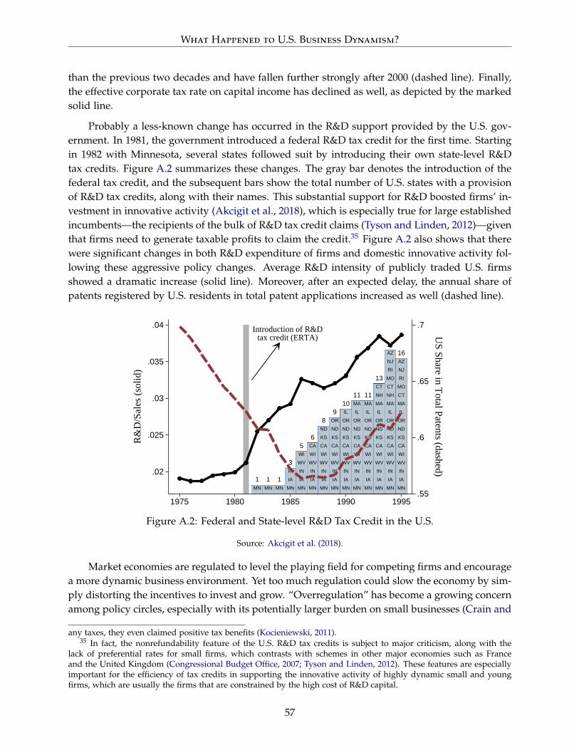
What Happened to U.S. Business Dynamism?
than the previous two decades and have fallen further strongly after 2000 (dashed line). Finally,the effective corporate tax rate on capital income has declined as well, as depicted by the markedsolid line.
Probably a less-known change has occurred in the R&D support provided by the U.S. gov-ernment. In 1981, the government introduced a federal R&D tax credit for the first time. Startingin 1982 with Minnesota, several states followed suit by introducing their own state-level R&Dtax credits. Figure A.2 summarizes these changes. The gray bar denotes the introduction of thefederal tax credit, and the subsequent bars show the total number of U.S. states with a provisionof R&D tax credits, along with their names. This substantial support for R&D boosted firms’ in-vestment in innovative activity (Akcigit et al., 2018), which is especially true for large establishedincumbents—the recipients of the bulk of R&D tax credit claims (Tyson and Linden, 2012)—giventhat firms need to generate taxable profits to claim the credit.35 Figure A.2 also shows that therewere significant changes in both R&D expenditure of firms and domestic innovative activity fol-lowing these aggressive policy changes. Average R&D intensity of publicly traded U.S. firmsshowed a dramatic increase (solid line). Moreover, after an expected delay, the annual share ofpatents registered by U.S. residents in total patent applications increased as well (dashed line).
Make America Great Again!
MN MN MN MNIAIN
IA
WIWV
MN
IN
WIWVIN
MN
CA
IA
KS
IA
CA
ND
MN
WVIN
WICA
IN
OR
WI
MNIA
NDKS
WVIN
CA
IA
WV
KSND
MN
WI
ORIL
IN
CA
OR
IAMN
ND
WV
KS
WI
KSCA
IN
WI
IA
IL
MN
WV
MA
ORND
IA
MA
MN
KS
ILOR
WV
CAWI
ND
CTNH
IN
MA
NJ
MO
KSCA
RI
IN
WI
MNIA
ND
IL
NH
OR
CT
WV
AZ
KS
WV
RI
WI
MNIA
OR
AZ
CTMA
ND
MO
NJ
IN
CA
IL
1 1 1
3
56
89
1011 11
13
1716
Introduction of R&Dtax credit (ERTA)
.55
.6
.65
.7
US Share in Total Patents (dashed).02
.025
.03
.035
.04
R&
D/S
ales
(sol
id)
1975 1980 1985 1990 1995Year
— R&D Intensity - - - Patenting Share of the U.S.Figure A.2: Federal and State-level R&D Tax Credit in the U.S.
Source: Akcigit et al. (2018).
Market economies are regulated to level the playing field for competing firms and encouragea more dynamic business environment. Yet too much regulation could slow the economy by sim-ply distorting the incentives to invest and grow. “Overregulation” has become a growing concernamong policy circles, especially with its potentially larger burden on small businesses (Crain and
any taxes, they even claimed positive tax benefits (Kocieniewski, 2011).35 In fact, the nonrefundability feature of the U.S. R&D tax credits is subject to major criticism, along with the
lack of preferential rates for small firms, which contrasts with schemes in other major economies such as Franceand the United Kingdom (Congressional Budget Office, 2007; Tyson and Linden, 2012). These features are especiallyimportant for the efficiency of tax credits in supporting the innovative activity of highly dynamic small and youngfirms, which are usually the firms that are constrained by the high cost of R&D capital.
57
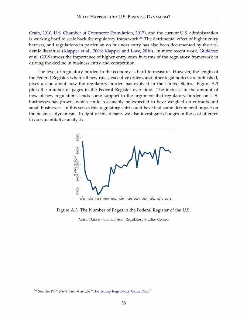
What Happened to U.S. Business Dynamism?
Crain, 2010; U.S. Chamber of Commerce Foundation, 2017), and the current U.S. administrationis working hard to scale back the regulatory framework.36 The detrimental effect of higher entrybarriers, and regulations in particular, on business entry has also been documented by the aca-demic literature (Klapper et al., 2006; Klapper and Love, 2010). In more recent work, Gutiérrezet al. (2019) stress the importance of higher entry costs in terms of the regulatory framework indriving the decline in business entry and competition.
The level of regulatory burden in the economy is hard to measure. However, the length ofthe Federal Register, where all new rules, executive orders, and other legal notices are published,gives a clue about how the regulatory burden has evolved in the United States. Figure A.3plots the number of pages in the Federal Register over time. The increase in the amount offlow of new regulations lends some support to the argument that regulatory burden on U.S.businesses has grown, which could reasonably be expected to have weighed on entrants andsmall businesses. In this sense, this regulatory shift could have had some detrimental impact onthe business dynamism. In light of this debate, we also investigate changes in the cost of entryin our quantitative analysis.
5000
060
000
7000
080
000
9000
0N
umbe
r of P
ages
1980 1983 1986 1989 1992 1995 1998 2001 2004 2007 2010 2013
Figure A.3: The Number of Pages in the Federal Register of the U.S.
Notes: Data is obtained from Regulatory Studies Center.
36 See the Wall Street Journal article “The Trump Regulatory Game Plan.”
58
What Happened to U.S. Business Dynamism?
B Additional Analytical Derivations
B.1 Evolution of µmt
µmt+∆t − µmt
∆t= xm−1tµm−1t − (x−mt + x−mt + δ) µmt (B.1)
µ1t+∆t − µ1t
∆t= (2x0t + x0t) µ0t + ((1− φ) x−2t + (1− φ) x−2t) µ2t − (x1t + x−1t + x−1t + δ) µ1t
(B.2)
µ0t+∆t − µ0t
∆t=
m
∑k=1
(φ f x−kt + φe x−kt + δ
)µkt + ((1− φ) x−1t + (1− φ) x−1t) µ1t − (2x0t + x0t) µ0t
(B.3)
B.2 Welfare
In the model economy, aggregate welfare over horizon T calculated at time t0 is given by
Wct0=∫ t0+T
t0
exp(−ρ (s− t)) log Ccs ds.
In Section 7, we report the difference in consumption-equivalent welfare between a counterfactualand the baseline economy using the following relationship:
∫ t0+T
t0
exp(−ρ (s− t0)) log Cnewcs ds =
∫ t0+T
t0
exp(−ρ (s− t0)) log((1 + ς)Cbase
cs
)ds. (B.4)
If a parameter change generates a new income sequence Cnewct between t0 and t0 + T satisfying
the above relationship, we say that the representative household in the counterfactual economyhas a ς% higher (lower) consumption-equivalent welfare over horizon T, with ς > 0 (ς < 0). Inother words, when ς > 0 (ς < 0), the representative consumer in the baseline economy wouldneed to receive ς% higher (lower) income at each point in time between t0 and t0 + T in order toobtain the same level of welfare it would have in the counterfactual scenario.
C Solution Algorithm
Before the discussion of the calibration results, a brief description of our solution algorithm isin order. The algorithm builds on the one developed by Akcigit et al. (2018), who construct anopen-economy version of the model considered here. Our aim to find the transition path thatemerges as the result of endogenous responses of firms to changes in parameters. We solve adiscretized version of the system. The solution algorithm assumes that the economy is initially
59
What Happened to U.S. Business Dynamism?
in the BGP and that the shocked parameter values converge to their new BGP value in T periods,where each period is divided into eight sub-periods. Notice that, due to the endogenous firmdecisions and the resulting endogenous adjustments in aggregate variables, the convergence ofthe economy the new BGP takes longer, which we assume to happen Tbgp > T periods. Thealgorithm is an iterative backward solution method (see Acemoglu et al., 2016). The progressionof the algorithm starts with solving for the terminal balanced growth path and then derives firmvalues and aggregate variables over the transition going backward from the terminal state. Asummary of steps is as follows.
1. Start with a guess of parameter values.
2. Compute the initial balanced growth path, where time derivatives are zero by definition.Compute the innovation rates, the implied growth rates, and finally the interest rate com-patible with balanced growth.
3. Compute the terminal balanced growth path in Tbgp defined by the terminal parametervalues similarly.
4. Next calculate the equilibrium over the transition. Guess a time path for the interest ratewith the terminal value set to its new BGP level. Solve for firm values and innovation ratesbackward in time starting from the terminal BGP.
5. Using the resulting sequences and starting from the initial gap distribution implied by theinitial BGP, simulate forward the income path and its growth rate. Use the Euler equationto derive the implied interest rate sequence and compare it to the series fed initially.
6. Update the guess for the interest rate series with the implied one and restart from step 2until the two converge. Once they do, use the final interest rate series and firm decisions tocompute the moments of interest.
7. Compare model-based moments to data targets. Search over the parameter space until thefollowing objective function (see Acemoglu et al., 2018) is minimized:
N
∑k=1
|model(k)− data(k)|12 |model(k)|+ 1
2 |data(k)| ,
where k denotes each moments and N is the number of targets.
60
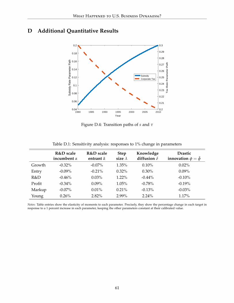
What Happened to U.S. Business Dynamism?
D Additional Quantitative Results
1980 1985 1990 1995 2000 2005 2010
Year
0.04
0.06
0.08
0.1
0.12
0.14
0.16
0.18
0.2
Sub
sidy
Rat
e P
aram
eter
Pat
h
0.2
0.21
0.22
0.23
0.24
0.25
0.26
0.27
0.28
0.29
0.3
Tax
Rat
e P
aram
eter
Pat
h
SubsidyCorporate Tax
Figure D.4: Transition paths of s and τ
Table D.1: Sensitivity analysis: responses to 1% change in parameters
R&D scaleincumbent α
R&D scaleentrant α
Stepsize λ
Knowledgediffusion δ
Drasticinnovation φ = φ
Growth -0.32% -0.07% 1.35% 0.10% 0.02%Entry -0.09% -0.21% 0.32% 0.30% 0.09%R&D -0.46% 0.03% 1.22% -0.44% -0.10%Profit -0.34% 0.09% 1.05% -0.78% -0.19%Markup -0.07% 0.01% 0.21% -0.13% -0.03%Young 0.26% 2.82% 2.99% 2.24% 1.17%
Notes: Table entries show the elasticity of moments to each parameter. Precisely, they show the percentage change in each target inresponse to a 1 percent increase in each parameter, keeping the other parameters constant at their calibrated value.
61