HCEO WORKING PAPER SERIES

Working Paper

The University of Chicago1126 E. 59th Street Box 107

Chicago IL 60637

www.hceconomics.org

Outside Options (Now) More Important than Race in

Explaining Tipping Points in US Neighborhoods

Peter Blair∗†

September 25, 2017

Abstract

I develop a revealed-preference method for estimating neighborhood tipping points.

I find that census tract tipping points have increased from 15% (1970) to 42% (2010).

The corresponding MSA tipping points have also increased from 13% (1970) to 35%

(2010). While tipping points are traditionally associated with the racial attitudes of

white households, I find that cross-sectional differences in MSA tipping points, going

from 1970-2010, depend less on differences in the racial attitudes of white households

and more on the outside options faced by white households. These results support a

continued role for place-based policies in mitigating residential segregation.

JEL Classification: R23, R21, J60

Keywords: preferences, race, Schelling model, tipping points, outside options.

∗Blair: Department Economics, Clemson University, pblair@clemson.edu and www.peterqblair.com†I received helpful comments from: Raj Chetty, William Darity Jr., Anthony Defusco, William Dougan,

Gilles Duranton, Steven Durlauf, Molly Espey, Fernando Ferreira, Robert Fleck, Edward Glaeser, JosephGyourko, Jessie Handbury, Joseph Harrington, Nathaniel Hendren, Damon Jones, Clarence Lee, GlennLoury, Corinne Low, Michael Makowsky, Conrad Miller, Albert Saiz, Mark Shepard, Curtis Simon, ToddSinai, Kent Smetters, Robert Tollison, Susan Wachter, Maisy Wong and the seminar participants at MIT,Wharton, Purdue, Swarthmore, Clemson, Emory, the Cleveland Fed, University of Chicago Summer Schoolfor Socioeconomic Inequality, the ASSA meetings, and the Southern Economic Association Conference.Mickey Whitzer, Kinde Wubneh, Lynn Selhat, Jennifer Moore, Julian Blair, Judith Blair, Rafael Luna (LunaScientific Story Telling) and Daniel DeVougas provided excellent help with preparation of the manuscript.All remaining errors are mine.

1

1 Introduction

A neighborhood tips when a marginal increase in its minority population leads to white flight

from the neighborhood. Given the link between racial segregation and adverse outcomes for

minorities, it is important to understand the mechanisms that drive neighborhood tipping.1

Furthermore, neighborhood tipping points can be important parameters for place-based poli-

cies like the Moving to Opportunity Experiment (MTO). In place-based programs where the

treatment is the destination neighborhood, it may be important to discern whether the act

of assigning minority households to a destination might itself result in the neighborhood

tipping, thereby undermining the intended treatment (Kling, Liebman, and Katz 2007).

Historically, the debate between economists and other social scientists on tipping centered

on whether neighborhood tipping reflects racial animus of non-minorities (whites) toward

minorities. In an early essay, “The Metropolitan Areas as Racial Problem,” University of

Chicago political scientist Morton Grodzins asserted that neighborhood tipping reflects “the

unwillingness of white groups to live in proximity to large numbers of [African Americans].”

Later work by economists, notably Thomas Schelling (1969, 1971), challenged this view,

demonstrating with a set of intuitive and simple models that segregation, at the neighborhood

and city levels, could occur even if white households, at the individual level, did not possess

a strong aversion to living in communities with minorities. One of the limitations of this

model, as Schelling himself noted, was that it did not include a role for outside options: “This

is but a small sample of possible results, using straight-line schedules and simple dynamics.

There are no expectations in the model, no speculation, no concerted action, no restriction

on the alternative localities available” (Schelling 1969).

The focus of this current paper is the role that outside options, i.e. the “alternative

localities available,” play in neighborhood tipping. The key insight of this paper is that

1Segregation impacts the provision of public goods to minorities, particularly if preferences for redistribu-tion are local (Zeckhauser 1993; Bayer, McMillan, and Rueben 2005). Additionally, residential segregationcreates spatial mismatches: minorities are disconnected from jobs, role models, and opportunities to interactwith non-minorities, which may result in the persistence of racial stereotypes (Kain 1968).

2

the tipping threshold for a non-minority household depends on its preferences for minority

neighbors and on the household’s outside options. In some cases, the dearth of preferable

outside options will result in a tipping threshold that is high (more racial integration is

tolerated) even though non-minority households have a strong relative preference for living

with other non-minorities. As an example, consider a city with a choice-set of two census

tracts: tract W, which is 100% non-minority, and tract M, which is 100% minority. Suppose

further that non-minority households in the city have a relative preference for non-minority

neighbors. What would happen if minorities were to integrate tract W? Would non-minority

households exit tract W in preference for tract M? Contrary to the intuition that a stronger

relative preference for same-race neighbors leads to more white flight, the stronger the white

household’s preferences for white neighbors, the more likely it will be to remain in tract

W even as the neighborhood integrates. In the same way that competition for employees

among firms sets the cost of discriminating against minority employees (Becker 1993), the

availability of preferable outside options sets the cost of acting on racial preferences in the

housing market.

I define a household’s neighborhood as the census tract where it resides, and its outside

options as the set of all of the other census tracts in its MSA of residence. I further impose

an incentive compatibility constraint on the exit decision of non-minority households. Non-

minority households exit their current neighborhood if exercising their outside option delivers

more utility than remaining in their current neighborhood. By imposing this constraint, I

am able to exploit sorting patterns in the data to estimate static tipping points at the

census tract level which are defined within the context of a discrete choice model of housing

(McFadden 1978; Berry, Levinsohn, and Pakes 1995; Bayer et al. 2007). The two main

contributions of this papers are: (i) I provide a method for computing census tract tipping

points (ii) I produce estimates of census tract tipping points for the census tracts of 123 US

cities that cover the five most recent censuses (1970-2010).

Computing tipping points for individual census tracts is a methodological contribution

3

to the empirical literature on tipping, which has progressed from the treating tipping as a

national phenomenon (Easterly 2009) to estimating tipping points at the MSA level (Card,

Mas, and Rothstein, 2008). In some cases, the distribution of census tract tipping points

is disperse and an MSA average may mask this heterogeneity. Mobile, AL and New Jersey

provide an illustrative case (Figure 1). In 1970, both cities have a mean MSA tipping point

of 22%. In Mobile, the dispersion about this mean is large, whereas for New Jersey there

is relatively less dispersion about this mean. As such, an MSA-wide place-based policy is

more likely to work consistently in New Jersey, whereas Mobile would require more locally

targeted policy to account for the heterogeneity in tipping points by census tract.

In computing the tipping points for the 38,466 tracts in my data, I find that the mean

neighborhood (tract) tipping point in the United States has increased at a rate of 6 percentage

points per decade – from 15% in 1970 to 42% in 2010. To compare these results with the

literature, I aggregate my tract tipping points to the city level and find that the mean

metropolitan statistical area (MSA) tipping points also increased at an average rate of 5

percentage points per decade from 13% (1970) to 35% (2010). According to other estimates

in the literature, the mean tipping point of US cities increased from 12% in (1970) to 14%

in (1990), an average of 1 percentage point per decade (Card, Mas, and Rothstein 2008). I

show that prior estimates understated city tipping points because they reflected the average

tipping points of the marginal census tracts in the city (i.e., those that were close to tipping),

whereas my estimates are an average of the tipping points of both the marginal and infra-

marginal census tracts in a city. One way to combine these two sets of results is that the

tipping point of the marginal census tract has changed gradually over time, whereas the

tipping point of the infra-marginal census tracts have increased more rapidly over time.

In the data, I also find evidence that cross-sectional differences in city tipping points

depend crucially on the outside options of non-minority households. Moreover, the relative

importance of outside options in explaining cross-sectional differences in city tipping points

vis-a-vis racial preferences is increasing over time. In 1970, a decrease of one standard de-

4

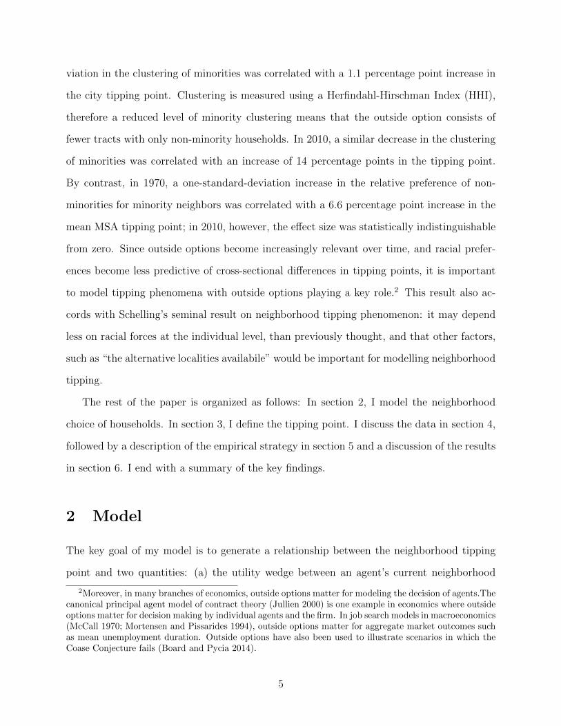
viation in the clustering of minorities was correlated with a 1.1 percentage point increase in

the city tipping point. Clustering is measured using a Herfindahl-Hirschman Index (HHI),

therefore a reduced level of minority clustering means that the outside option consists of

fewer tracts with only non-minority households. In 2010, a similar decrease in the clustering

of minorities was correlated with an increase of 14 percentage points in the tipping point.

By contrast, in 1970, a one-standard-deviation increase in the relative preference of non-

minorities for minority neighbors was correlated with a 6.6 percentage point increase in the

mean MSA tipping point; in 2010, however, the effect size was statistically indistinguishable

from zero. Since outside options become increasingly relevant over time, and racial prefer-

ences become less predictive of cross-sectional differences in tipping points, it is important

to model tipping phenomena with outside options playing a key role.2 This result also ac-

cords with Schelling’s seminal result on neighborhood tipping phenomenon: it may depend

less on racial forces at the individual level, than previously thought, and that other factors,

such as “the alternative localities availabile” would be important for modelling neighborhood

tipping.

The rest of the paper is organized as follows: In section 2, I model the neighborhood

choice of households. In section 3, I define the tipping point. I discuss the data in section 4,

followed by a description of the empirical strategy in section 5 and a discussion of the results

in section 6. I end with a summary of the key findings.

2 Model

The key goal of my model is to generate a relationship between the neighborhood tipping

point and two quantities: (a) the utility wedge between an agent’s current neighborhood

2Moreover, in many branches of economics, outside options matter for modeling the decision of agents.Thecanonical principal agent model of contract theory (Jullien 2000) is one example in economics where outsideoptions matter for decision making by individual agents and the firm. In job search models in macroeconomics(McCall 1970; Mortensen and Pissarides 1994), outside options matter for aggregate market outcomes suchas mean unemployment duration. Outside options have also been used to illustrate scenarios in which theCoase Conjecture fails (Board and Pycia 2014).

5

and his/her outside options; and (b) the marginal utility for minority neighbors. The model

consists of a demand side, in which households have neighborhood preferences that depend

on the endogenous racial mix of the neighborhood and the price of housing services in the

neighborhood, as well as other amenities therein. I follow the literature in focusing on the

demand side and abstracting from the influence of changes in housing supply on tipping

points (Card et. al. 2008, Caetano and Maheshri 2013).

A household’s choice-set consists of all of the census tracts in its MSA. Accordingly,

its outside option consists of all of the tracts in its MSA excluding its current tract of

residence. In cities where there are many minority tracts, the outside option will impact

the ability of non-minorities to exit their neighborhoods of residence. With this definition of

households choice-set, I use a discrete choice model to exploit within-MSA sorting patterns

in the data to obtain tipping points for each census tract-year observation (McFadden 1978;

Berry, Levinsohn, and Pakes 1995; Bayer et al. 2007). I use data from N census tracts in

an MSA from two consecutive census periods to estimate 2N tipping points – one for each

census-tract-year observation. Using the approach in Card et. al. (2008) and similar data

generates a single tipping point – the MSA tipping point.

In the model, I construct the tipping point in two steps. First, I use the estimates of the

sorting model to compute an exit function of white households from the neighborhood. For

a given exogenous change in the mean utility of whites in neighborhood, τ , the exit function

measures the probability that a white household exits its current neighborhood for its best

alternative in its choice-set. I refer to τ as the utility tolerance of white households since

it parametrizes the exit probability as a function of changes in the mean utility of whites.

At the tipping point, the first derivative of the exit function, the exit rate, equals zero, and

the tolerance equals τ ∗. This definition of tipping is similar to the approach in Card et al.

(2008), which associates the tipping point with the share of minorities for which the rate

of decline in white population is maximal. I get the tipping point by converting the utility

tolerance into a percent minority by using an empirical relationship between the percent

6

minority and the mean utility.

2.1 Demand Side

In the model, there are C cities indexed c ∈ {1, 2, ..., C}, and two types of households

that are differentiated by a type index, r ∈ {w,m}. The type index r = w references

white households, while the type index r = m references minority households. Each city is

exogenously assigned a total of Qwtot white households and total of Qm

tot minority households.

Each household, in turn, endogenously sorts into one of the N neighborhoods in that city,

indexed by n ∈ {1, 2, ..., N}. The sorting of households to neighborhoods depends on the

household income, the price of housing in equilibrium, and the equilibrium level of amenities

in each of the N neighborhoods.

A household’s problem is to choose the neighborhood that delivers the maximum utility.

Solving the household’s problem requires first solving for the indirect utility for each of the N

possible neighborhoods, and then choosing the neighborhood that delivers the maximum in-

direct utility. Households h of type r have utility over neighborhood amenities, consumption,

and housing services in each neighborhood n. The utility function takes the form:

Uhnr = log(Ahnr)︸ ︷︷ ︸Amenities

+αlog(Chnr)︸ ︷︷ ︸Consumption

+ βlog(Hhnr)︸ ︷︷ ︸Housing

, for r ∈ {w,m}. (1)

The parameters α and β are the consumption and housing shares. The neighborhood

amenity, Ahnr, consists of an endogenous component and an exogenous component in addi-

tion to an idiosyncratic taste shock:

log(Ahnr) = γrfn︸︷︷︸Endog. Amenity

+ θX︸︷︷︸Exog. Amenities

+ ξn︸︷︷︸Unobs. Quality

+ εhnr︸︷︷︸Taste Shocks

. (2)

The endogenous amenity is the racial composition of neighborhood, fmn = Qm

n

Qmn +Qw

n, which

is the percent minority in the neighborhood. The value of the endogenous amenity varies

7

by agent type, with whites valuing a one percentage point increase in the minority share by

an amount γw, and minorities valuing a one percentage point increase in the minority share

by an amount γm. The X’s represent observable characteristics of the neighborhood, which

also capture the overall quality of the neighborhood and the ξnr unobservable measures of

neighborhood quality, which may vary by race. I assume that the taste shocks are i.i.d. and

follow a type 1 extreme value distribution. This assumption makes it convenient to obtain

closed-form solutions without compromising the key insight of the model – which is that

the choice-set of white agents impacts the neighborhood tipping points – and allows for the

estimation of sub-MSA tipping points.

2.1.1 Solving for the Indirect Utility of a Neighborhood

For each neighborhood n households choose a bundle of consumption Chnr and housing Hhnr

to maximize utility, subject to the household’s budget constraint:

Chnr + pnHhnr ≤ Ih. (3)

Consumption is the numeraire good, and housing price pn is in terms of units of consumption.

The household’s income Ih is exogenously determined and independent of the household’s

choice of a neighborhood n. For neighborhood n, the optimal bundle (C∗hnr, H∗hnr) is:

C∗hnr =

(αr

αr + βr

)Ih (4)

H∗hnr =

(βr

αr + βr

)(Ihpn

), (5)

and the associated indirect utility is:

Vhnr = γr

(Qm

n

Qmn +Qw

n

)+ (αr + βr)log(Ih)− βrlog(pn) +Xθ + ξn + εhnr. (6)

8

To simplify notation, I define Vhnr, the deterministic part of the indirect utility, using the

following relation:

Vhnr = Vhnr + εhnr. (7)

2.1.2 Solving for Neighborhood Demand

After having solved for the indirect utility for each neighborhood, each household of income

Ih and type r chooses the neighborhood, n∗hr, that delivers the highest indirect utility:

n∗hr = arg max{Vhnr} (8)

The household’s utility-maximizing behavior across the N neighborhoods in the city generates

a conditional demand function, Qrn (~p| Ih), for each neighborhood by both household type

and household income category Ih. The conditional demand functions take the form:

Qrn (~p|Ih) = Qr

tot

exp(Vhnr)N∑

n′=1

exp(Vhn′r)

, for r ∈ {w,m}, (9)

where ~pn = {p1, p2, ..., pN} is the vector of house prices for all neighborhoods in the city.

The unconditional demand for neighborhood n by households of type r equals the sum of

the conditional demand functions over the income categories:

Qrn ( ~pn) =

∑h

Qrn (~p|Ih), for r ∈ {w,m} (10)

3 Tipping Point

In the empirical literature on tipping, the tipping point of a neighborhood n is defined by

a threshold minority fraction, f ∗n. When the minority fraction of the neighborhood exceeds

this threshold, whites exit the neighborhood at a rapid rate. Below this threshold, changes

9

in the white population of the neighborhood are less stark. In the context of this model,

I define the tipping point of a neighborhood as corresponding to the minority fraction for

which the exit rate of whites from the neighborhood is maximal.

In order to compute the tipping point, I first construct the exit function for each neigh-

borhood. This exit function traces out the probability of white flight from the neighborhood

n as a function of the decrease in utility experienced by whites in the neighborhood due to

the arrival of minorities. I adopt a similar approach to Caetano and Maheshri (2013) by us-

ing counter-factual decreases in the utility of whites to construct the exit function. The exit

function also depends on the utility wedge between the households inside option, Vhnw, and

the household’s next best alternative, Vha(n)w, where the notation a(n) is the neighborhood

that is the households best alternative, should it choose to relocate to another census tract

in the same MSA.

After constructing the exit probability as a function of the counter-factual decrease in

utility, I will solve for the utility of whites in the neighborhood at the tipping point by

solving for the inflection point of the exit function: the level of utility for which the second

derivative of the exit function is zero. The first derivative of the exit function is the exit

rate. The second derivative, which is required to solve for the inflection point, captures the

marginal exit rate. When the marginal exit rate equals zero, the exit rate is maximal.

3.1 Conditional Exit Functions

Following the arrival of new minority households to a neighborhood n, some white households

may find it preferable to exit the neighborhood and relocate to the best alternative among the

other N-1 neighborhoods in its city, neighborhood a(n), instead of remaining in neighborhood

n. I use τnw to represent the loss in indirect utility that white households of income category

h experience due to the arrival of new minority households to their host neighborhood n.

The conditional exit function of whites, which represents the exit probability of whites of a

10

given income category, is given by:

E(τnw; ~V |Ih) =∑a(n)

Prob(Vhnw − τnw + εnhnw < Vha(n)w + εha(n)w)︸ ︷︷ ︸Prob. exit n for a(n)

× ωa(n)︸︷︷︸Prob. a(n) is best opt.

(11)

=∑a(n)

∞∫−∞

F (Vha(n)w − Vhnw + τnw + εha(n)w)f(εha(n)w)dεha(n)w

ωha(n)w

,

(12)

where ωha(n)w is the probability that neighborhood a(n) ∈ {1, 2, ..n−1, n+1, ...N} is the best

alternative among the N-1 options in the household’s choice-set, and F (·) is the cumulative

distribution function for the taste shocks, which I assume follow a type 1 extreme value

distribution. The probability weight ωha(n)w is assumed to be the share of whites in the

alternative neighborhood a(n) relative to the total number of whites in the MSA excluding

the current tract n:

ωha(n)w =exp(Vha(n)w)∑

a∈{a(n)}exp(Vhaw)

. (13)

Each non-minority household living in a given tract will have a single best alternative.

However, since I do not observe all of the covariates of an individual non-minority household,

I average over all the non-minority households in a neighborhood to obtain a probability than

a given tract in the MSA is best alternative for non-minority households in this tract. The

probability weights in equation (13) are type of counter-factual market shares for utility

maximizing non-minority households who face a choice-set of the N-1 census tracts in the

MSA, where census tract n has been excluded from consideration. As such these weights

present the probability that a tract a(n) is the best option of the N-1 tracts for non-minority

households. Since I have assumed that preferences are homogeneous with-in racial group,

but heterogeneous across racial group, these probability weights are natural measures of the

probability that tract a(n) is the best alternative for a moving agent.3

3This assumption is particularly reliable for cases where there are a large number of census tracts in theMSA. In these cases, the removal a single census tract has a diminishing effect on the overall sorting in the

11

3.2 Unconditional Exit Function

The unconditional exit probability of whites from neighborhood n is the sum of the con-

ditional exit functions weighted by the number of households in the income category that

corresponds to the individual conditional demand functions, Qwhn, as a fraction of the total

number of whites in neighborhood n, Qwn :

E(τnw; ~V ) =15∑h=1

(E(τnw; ~V |Ih) · Q

whn

Qwn

)(14)

The unconditional exit function will be dominated by the behavior of whites in the most

highly represented income categories in the neighborhood. This is captured in the weighting.

As the utility drop becomes large and positive, due to the arrival of minorities, the exit prob-

ability goes to one, and all whites exit the neighborhood. In the opposite limit, as τnw gets

arbitrarily large and negative, which corresponds to whites moving into the neighborhood,

the probability of white residents exiting the neighborhood converges to zero. In general,

the exit function will resemble an S-curve with τnw on the horizontal axis and the associated

conditional exit probability on the vertical axis.

3.3 Tipping Point

The tipping point of the neighborhood is the percent minority at the inflection point of the

exit function. This is the point at which the exit function changes concavity and the exit

rate (the derivative of the exit function with respect to τnw) is maximal:

d2E(τ ∗nw; ~V )

dτnw2= 0. (15)

At the tipping point, the mean utility of white households in neighborhood n has de-

creased by an amount −τ ∗n. I use the the relative marginal utility for minority neighbors to

MSA as the number of tracts in the MSA increases. In the paper, we follow the literature and restrict ouranalysis to MSAs with at least 100 census tracts (Card et. al. 2008).

12

convert this decrement in mean utility into a change in the percent minority. Accordingly,

the percent minority at the tipping point is given by:

f ∗n = fn −τ ∗n

γw − γm(16)

The first piece of the tipping point is the initial percent minority in the census tract,

fn = Qmn

Qmn +Qw

n. The second part of the tipping point is the change in the percent minority

that takes the neighborhood to the critical point of the exit function. The key take-away

from equation (16) is that the tipping point is directly proportional to the utility tolerance

of non-minorities for minorities, τ , and inversely proportional to the relative preference of

non-minority households for minority neighbors, γw − γm, which in the data is negative. If

τ ∗n > 0, then the neighborhood n is a more desirable neighborhood than the alternatives in

the choice-set. In order for this neighborhood to tip, minorities must move in to lower the

utility of non-minorities to the point where the neighborhood tips. If τ < 0, the opposite

is true, and the tipping point is lower than the current fraction of minorities. One merit of

estimating tipping points in this manner is that it allows researchers to estimate the tipping

point of census tracts that have tipped, that have yet to tip (τ > 0), and that are beyond

their tipping points (τ < 0).

3.3.1 Estimating Preferences

This preference parameter, γw−γm, is identified from the differential sorting of non-minorities

into neighborhoods as a function of the fraction of minorities in the neighborhood. From

equation (6), we relate the ratio of the non-minority to minority market share of a neigh-

borhood to the percent minority in the neighborhood and the relative preference parameter

γw − γm:

log

(Qw

n

Qwtot,c

)− log

(Qm

n

Qmtot,c

)= (γw − γm)

(Qm

n

Qmn +Qw

n

)+ en,m (17)

13

The term on the left-hand side is the relative market share of whites to minorities in

neighborhood n. The market share of a neighborhood is the fraction of households in the

MSA of a given type that reside in the neighborhood. Moreover, the log of the market share

is mean utility of an household of the given racial type. The regressor on the right-hand

side is the percent minority in the census tract. By taking the relative market share, I

can difference out characteristics of the neighborhood that are valued equally by minorities

and non-minorities. Here I make the assumption that white and minority households value

everything similarly except the percent minority in the tract.

3.4 Semi-Parametric Estimate of Tipping Point

I also use the relative market shares to develop a semi-parametric estimator of the tipping

point, which is non-linear parallel to equation (16). In equation (17), the relative market

shares are a linear function of the fraction of minorities, fn. One limitation of this speci-

fication is that it can produce tipping points that lie outside of the interval [0, 1]. I relax

this assumption by allowing the percent minority in a neighborhood to depend flexibly on

the relative market shares. I obtain this relationship, empirically, by regressing the percent

minority in the census tract on powers of the log of the relative market shares:

Qmn

Qmn +Qw

n

= α0 +5∑

j=1

αj

[log

(Qw

n

Qwtot,c

)− log

(Qm

n

Qmtot,c

)]j︸ ︷︷ ︸

ratio of white:minority market share

(18)

The coefficients of this regression define the inverse mapping from the ratio of the non-

minority to minority market shares to the percent minority in the tract. This inverse mapping

is important because I have calculated the mean utility of white households at the tipping

point, but the ultimate quantity of interest is the percent minority, which defines the tipping

point; therefore we need the inverse mapping of the relative utility to percent minority. I use

the estimated parameters to obtain the percent minority at the tipping point by inserting a

value of Vnw − τ ∗nw − Vnm = log(

Qwn

Qwtot,c

)− log

(Qm

n

Qmtot,c

)− τ ∗nw for the relative market share at

14

the tipping point.

4 Data

To estimate the model, I use data from the U.S. census covering five decades: 1970, 1980,

1990, 2000, and 2010. This data consists of the demographic characteristics of the households

living in each of the census tracts, as well tract-level measures of the local housing stock and

local economic conditions. The key variables of interest for this study are the population

shares of each census tract broken down by race. Prior work has used similar data from the

1970-2000 extracts of the census data to compute MSA tipping points (Card et al. 2008).

I build on this work by updating the previous results to include estimates of tipping points

from the 2000 and 2010 censuses. With these five decades of tipping points, I trace the time

evolution of tipping points to show that, over time, tipping points in the United States have

increased. In addition to this empirical contribution, my paper also makes a methodological

contribution. Whereas these data have been used in Card et. al. (2008) to compute MSA

tipping points, I use these data to compute census tract tipping points. These tract-level

estimates capture the distribution of neighborhood tipping points within an MSA.

I follow Card et al. (2008) in making the following cuts in the data. First, I eliminate

any tracts whose population growth between consecutive census years surpasses average

population growth in the MSA by more than five standard deviations. Second, I drop all

tracts that experience an increase of more than 500% in their white population between

consecutive census years. These first two cuts reduce the effect of outliers on the results of

this study. For the final cut, I focus my analysis on MSAs that have 100 census tracts or

more, also following Card et al. (2008). There are 123 MSAs that satisfy these criteria, and

these MSAs cover the 38,489 census tracts that comprise my final data set.

15

5 Results

5.1 Descriptive Statistics: Racial Preferences

In Table 1, I report the mean, median, and standard deviation of these relative preference

estimates from the “diff-in-diff” procedure of equation (17). To compute standard errors on

the point estimate and preference parameters, I use an N=1000 bootstrap. The estimates for

γw−γm range from -8.84 in 1970 to -6.11 in 2010. For 1970, the diff-in-diff point estimate of

-8.84 means that a 7.8 percentage point increase in the fraction of minorities was associated

with a 50% reduction in the non-minority population of the average neighborhood. The

diff-in-diff point estimate of -6.11 for 2010 indicates that an 11.3 percentage point increase

in the fraction of minorities was needed for the non-minority population in a neighborhood

to halve.

In Figure 2, I graph decadal changes in the distribution of the relative racial preferences.

Each of the kernel density plots uses data from the 5th to 95th percentile to limit the effect

of outliers on the shape of the graphs. In each ten-year period, the distribution of preferences

shifts to the right, indicating that the mean is decreasing over time. A decreasing mean over

time is consistent with white households becoming more tolerant of living with minorities.

Over time, the distribution of preferences also narrows. This suggests that, on average, white

households increase in tolerance is occurring across all levels of the preference distribution.

The compression in the distribution of racial preferences across cities, over time, is responsible

for the declining importance of racial preferences as an explanatory factor in cross-sectional

differences in tipping points across cities.

5.2 Descriptive Statistics: Tipping Points

By applying the model to the data, I obtain two sets of census tract tipping points. The first

set comes from the the linear model in equation (16), and the second set comes from the

semi-parametric estimator of equation (18). Since the predicted outcome of both approaches

16

is a tipping point that lies in the interval [0,1], an apt analogy for describing the two methods

is that the linear (diff-in-diff method) is analogous to a linear probability model, while the

semi-parametric method is analogous to a non-linear, e.g. probit model, which produces

estimates that lie in the interval [0,1].

5.2.1 Tract Tipping Points

In Table 2, I report summary statistics for the census tract tipping points from the diff-in-diff

method of equation (16). The table is divided into three panels. In the first panel I report

the mean, median, and standard deviation of the census tract tipping points for the full

sample in each of the census years. In the second panel I report the identical statistics for

the census tract tipping points that are in the allowable [0,1] range for the given census year.

In the third panel, I report the identical statistics for each census tract that is in range in

2010. This restriction gives a consistent set of tracts across all census years. Because some of

the tipping points are not “in range,” I use the results from these three panels as checks that

the time trends in the tipping points that I observe are consistent under the three sample

restrictions: the full sample, the sample of tracts that are in range in the census year, and

a consistent set of tracts that are required to be in range in the 2010 census year. In Table

3, I present results from the semi-parametric (inverse) method of equation (18).

The mean and median of the census tract tipping points increase monotonically over time

for both the diff-in-diff and the semi-parametric (inverse) mapping methods. Moreover, the

mean tipping point is greater than the median tipping point for all years. The magnitudes of

the estimates are also comparable in both methods. I focus my discussion on the estimates

from the inverse mapping method, because between 98% and 99.6% of the tipping points

for this method are in the allowable [0,1] range.4 For this method the tipping points have

a mean of 15% in 1970, 22% in 1980, 28% in 1990, 36% in 2000, and 41% in 2010. The

median-tract tipping point also monotonically increased from 1970 to 2010. In 1970, the

4By comparison, only 57%-84% of the diff-in-diff linear estimates are in range. Nevertheless, the resultsin the second panel of Table 2 agree with the results in the inverse mapping method for all years.

17

median-tract tipping point was 13% and by 2010 it was 34%. The inter-censal correlation

between the tract tipping points is between 0.71 and 0.78, as reported in Table 4. This

demonstrates that while the mean tipping points of the tracts has increased over time, there

has been strong persistence in the ranking of tracts across time.

In Figure 3, I report kernel density plots of the tract tipping points in each census year.

The distribution for each year is a single peaked distribution that is left skewed. Over time

the peak pushes out the right, and the distribution flattens and gains more mass in the

right tail. With each succeeding census year the curve shifts out by less, indicating that the

tipping point is increasing at a decreasing rate.

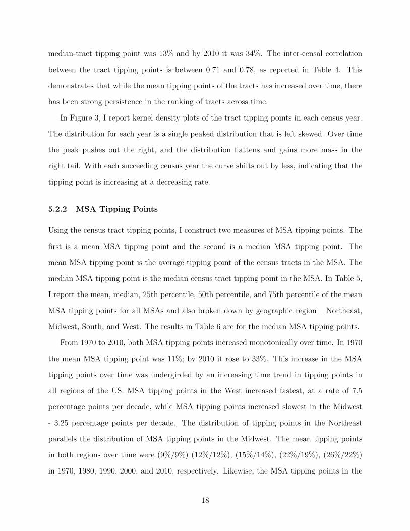
5.2.2 MSA Tipping Points

Using the census tract tipping points, I construct two measures of MSA tipping points. The

first is a mean MSA tipping point and the second is a median MSA tipping point. The

mean MSA tipping point is the average tipping point of the census tracts in the MSA. The

median MSA tipping point is the median census tract tipping point in the MSA. In Table 5,

I report the mean, median, 25th percentile, 50th percentile, and 75th percentile of the mean

MSA tipping points for all MSAs and also broken down by geographic region – Northeast,

Midwest, South, and West. The results in Table 6 are for the median MSA tipping points.

From 1970 to 2010, both MSA tipping points increased monotonically over time. In 1970

the mean MSA tipping point was 11%; by 2010 it rose to 33%. This increase in the MSA

tipping points over time was undergirded by an increasing time trend in tipping points in

all regions of the US. MSA tipping points in the West increased fastest, at a rate of 7.5

percentage points per decade, while MSA tipping points increased slowest in the Midwest

- 3.25 percentage points per decade. The distribution of tipping points in the Northeast

parallels the distribution of MSA tipping points in the Midwest. The mean tipping points

in both regions over time were (9%/9%) (12%/12%), (15%/14%), (22%/19%), (26%/22%)

in 1970, 1980, 1990, 2000, and 2010, respectively. Likewise, the MSA tipping points in the

18

South mirrored those in the West.

The MSA tipping points exhibited a high degree of correlation across consecutive census

periods, notwithstanding the fact that they increased substantially across time (Table 7).

One striking fact about the MSA tipping points is that the mean MSA tipping points and the

median MSA tipping points had very similar distributions. For example, in the full sample

the mean of the mean MSA tipping points and the mean of the median MSA tipping points

were (13%/11%), (18%/16%), (22%/21%), (30%/28%), and (35%/33%) in 1970, 1980, 1990,

2000, and 2010, respectively. For each year the difference between the mean and the median

MSA tipping points was between 1 and 2 percentage points.5 Moreover, the mean of the

mean MSA tipping points is similar to the median of the census tract tipping points. I

exploit this fact in the next section, where I show that the tipping points estimated by Card

et al. (2008) are similar to the local mean and the local median of the tipping points of the

marginal census tracts in the MSA.

5.3 Comparison with Prior Estimates of Tipping Points

The Card et al. 2008 (CMR) tipping points cover three decades – 1970, 1980, and 1990. On

average, the tipping points that I get are 3 percentage points higher in 1970, 9 percentage

points higher in 1980, and 12 percentage points higher in 1990 than CMR. This difference

occurs because the two tipping points capture different aspects of the underlying distribution

of census tract tipping points. The MSA tipping points that I report are an average of the

underlying census tract tipping points, which I am able to estimate because I model the

location decision of households within the MSA and use the counter-factual exercise to

obtain census tract tipping points. The CMR approach accurately measures a local average

of the marginal census tracts (i.e., tracts that are close to the tipping threshold). This

distinction between the two MSA tipping points is evident from the theories guiding their

5By comparison, the mean and median of the census tract tipping points were more dissimilar (15%/13%),(22%/16%), (28%/21%), (36%/28%), and (41%/34%) in the respective census years. For each year thedifference between the mean and the median tract tipping points is between 2 and 8 percentage points.

19

construction.

The CMR tipping points are the result of a fixed-point procedure. To obtain the MSA

tipping point, the CMR fits a polynomial of the change in the percent of whites between

census years (above the MSA average) as a function of the fraction of minorities in the base

census year. Each observation used to fit this function is a census tract in the MSA which is

appears into consecutive periods. The first method for determining the tipping point is to

solve for the zeros of this polynomial. The key point is that tracts below the tipping point

experience above-average growth in their non-minority (white) populations, whereas tracts

beyond the tipping point experience below average growth in their non-minority populations.

The minority fraction at the zero of this polynomial is taken to be the MSA tipping point.

In cases where there are multiple zeros, the authors took the zero that delivered the most

negative first derivative. This equilibrium selection procedure parallels the approach that I

take in this paper, where for each tract I stipulate that the tipping point occurs at the level

of utility for which the exit rate of non-minorities is maximal (and the marginal exit rate

equals zero). Since the CMR tipping point is the zero of a fitted polynomial, it depends

crucially on the behavior of the census tracts in the vicinity of this zero. I call these census

tracts the “marginal census tracts.” These are tracts that are close to their tipping points.

I call tracts that are farther away from the zero of the polynomial “infra-marginal census

tracts” because changes in the behavior the infra-marginal tracts have less bearing on the

estimated value of the CMR MSA tipping points.The setup of the CMR procedure suggests

that the CMR tipping points are local averages of the tipping points of the marginal tracts,

or perhaps the median of the tipping points of the marginal census tracts in the MSA. Since

I have estimates of tipping points for each census tract in an MSA, I can test the hypothesis

that the CMR tipping points are local averages of the tipping points of marginal census

tracts or the median of the tipping points of the marginal tracts.

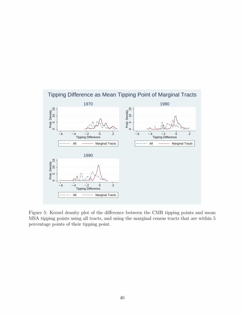
In Table 8, I present results from a regression of the difference between the CMR and

20

Revealed-Preference (PR) MSA tipping points, which I call the tipping difference,6 and the

fraction of marginal census tracts in the MSA. Here, a marginal census tract is a tract whose

percent minority is within 5 percentage points of its estimated tract tipping point. For

example, if a tract has a tipping point of 35% and a current percent minority of 32% it

is considered a marginal tract. Likewise, if another tract in the same MSA has a tipping

point of 7% and a current percent minority of 11%, I also consider it a marginal tract. To

allow for asymmetry in the impact of marginal tracts that lie to the left and to the right of

their respective tipping points, I include separate explanatory variables for (a) the fraction of

tracts in the MSA that are marginal and have minority fractions below their tipping points;

and (b) the fraction of tracts in the MSA that are marginal and have minority fractions

greater than their tipping points.

The constant terms from the regressions in Table 8 capture the mean tipping difference.

In 1990, the tipping difference was -15%. It was -10% in 1980 and -8% in 1970. These

regression results accord with the -13%, -9%, and -3% tipping differences from the raw data.

Based on the regression results, the marginal tracts that were below the tipping point drove

the tipping difference in 1990 and 1980. In 1970, the marginal tracts that were above the

tipping point (i.e., those that had already tipped), drove the tipping difference. One reason

there is a tipping difference at all is that there were few marginal tracts, and so an average

of the marginal tracts is different from an average of all tracts. To illustrate this point, I

combine the constant term from the regression and the significant coefficient on the marginal

tracts to compute the threshold fraction of marginal tracts, f required for there to be no

tipping difference in each year:

f =# marginal tracts in MSA

Total # tracts in MSA. (19)

To solve for f , I set the sum the constant term from the regression and the product of the

6I do not call this quantity a bias because my hypothesis is that the CMR tipping points measure thedistribution of the marginal census tracts, which in and of itself is an important quantity. We care aboutwhich tracts are marginal and how the distribution of marginal tracts varies across time and across space.

21

(significant) coefficient on the marginal tracts times f equal to zero. At this value of f , the

tipping difference is zero, and the CMR tipping points and the tipping points that I obtain

are equal. In 1990, 72% of the tracts would have to be marginal for there to be no tipping

difference. In 1980, 53% of the tracts would have to be marginal; and in 1970, 13% of tracts

would have to be marginal. In the reality, the average MSA consisted of 14% of marginal

tracts (below) in 1990, 13% of marginal tracts (below) in 1980, and 11% of marginal tracts

(above) in 1970. Since the mean number of marginal tracts was closest to the required level

in 1970, it is not surprising that the tipping difference was smallest in 1970. The opposite is

true for 1990, the year when the difference between the required threshold and the fraction

of tracts that were marginal was largest.

To verify this, I perform a similar exercise, this time changing the definition of the tipping

difference to be the difference between the CMR tipping point and the tipping point of the

median census tract in each MSA. When I restrict the sample to only the marginal tracts,

the tipping difference equals the difference between the CMR tipping point and the median

tipping point of the marginal census tracts. Apart from this change in the definition of the

tipping difference, Figure 6 is laid out identically to Figure 5. The dashed lines peak to

the left of zero, reflecting the fact that the CMR tipping points are smaller, on average,

than the MSA tipping points that I compute from the median. The solid lines, however,

peak even more sharply around zero than the solid lines using the mean. This reflects the

fact that the tipping difference also disappears when I compute MSA tipping points using

only the marginal tracts. With this sample restriction, the tipping difference of the median

MSA is reduced from -11.2% to -1.7% in 1990, from -7.8% to 0.1% in 1980, and does not

substantively change in magnitude in 1970 (from -3.7% to 4%). Taking the best of the local

mean and median results, the tipping difference of the median MSA is bounded above by

1.9% and bounded below by -0.1%. These results provide further support for the hypothesis

that the CMR tipping points capture the shape of the distribution of marginal census tracts

in an MSA.

22

From this comparison of marginal and infra-marginal tracts, we learn that the tipping

points of the marginal census tracts evolve more slowly over time than those of the infra-

marginal tracts. The CMR tipping points, which were shown to be an average of the marginal

tipping points, increased an average of 1 percentage point per decade (1970–1990). We also

learn that the infra-marginal tracts play an important role in the secular time trend of

tipping points. The MSA tipping points using all tracts (both marginal and infra-marginal)

increased at an average rate of 5.5 percentage points per decade (1970–2010), which is

substantially higher than the growth rate of the tipping points of infra-marginal tracts. An

important contribution of the method in this paper is that it enables researchers to compute

the tipping points of all census tracts and derived MSA tipping points, which are aggregates

of the underlying census tract tipping points. The dynamics of these MSA tipping points

better reflect the dynamics of the underlying census tracts.7

5.4 Results: Preferences versus Outside Options

The motivating insight of this paper is that outside options affect the ability of households

to act on their preferences for neighborhood racial composition. A household may remain

in a neighborhood despite its racial composition if the outside options do not offer higher

utility. The reverse is also true – a household may exit its current neighborhood because

of the availability of desirable alternative neighborhoods in its city. For each census year,

I decompose the mean MSA tipping point into a component due to the mean preferences

of the households and a measure of their outside options, which depends on the extent of

clustering in the city by race.

To measure minority clustering, I use a Herfindahl-Hirschman Index (HHI) that is stan-

dardized to have a mean of zero and standard deviation of one. To compute the index,

I construct the minority market share of each census tract n in a given census year y by

dividing the number of minorities in the tract by the total number of minorities in its MSA

7The mean tipping point of census tracts in the data increased by 6.75 percentage points per decade(19702010)

23

c: scn,m,y =Qc

n,m,y

Qctot,m,y

. I then square the minority market shares, sn,m,y and sum over them for

each MSA, c, to get the MSA HHIc :

HHIc =∑n

(scn,m,y)2. (20)

Finally, I de-mean the Minority HHI and normalize it to have variance 1 in each year. This

yields a minority HHI z-score,(HHIcm,z,y) for each MSA for each census year from 1970 to

2010. I construct a standardized non-minority HHI using an identical procedure (HHIcw,z,y).

To construct the standardized measure of racial preferences, (∆γcz,y), I de-mean the relative

marginal utility for minority neighbors from the diff-in-diff procedure of equation (17) and

normalize it to have standard deviation 1.

A one standard deviation decrease in the minority HHI corresponds to less clustering of

minorities in the MSA, or more census tracts in the MSA having some minority households.

Less clustering of minorities creates a choice-set in which many census tracts are sprinkled

with at least some minorities, making it difficult for non-minority households to sort into

all-white neighborhoods. A one standard deviation increase in the non-minority HHI corre-

sponds to more clustering of non-minorities into fewer census tracts within an MSA. Greater

clustering of non-minorities creates a choice-set that is potentially bimodal, with some tracts

having many non-minorities and others having few non-minorities. A one standard devia-

tion increase in the race preferences is associated with non-minorities having preferences for

minority neighbors that is more similar to the preferences that minorities have for minority

neighbors.

In Table 9, I report the results of a regression of mean MSA tipping points (T cy ) on

the minority HHI (HHIcm,z,y), the non-minority HHI (HHIcw,z,y), and the standardized race

preferences (∆γcz,y):

T cy = ηy1HHI

cm,z,y + ηy2HHI

cw,z,y + φy∆γcz,y. (21)

Since the tipping points were constructed using the choice-set faced by households and

24

the estimated preferences, I read this regression as providing a decomposition of the MSA

tipping points into a component due to the configuration of the outside option and the

mean preferences in the MSA. The results of this regression are summarized in Figure 7.

The first result is that less minority clustering, or having the presence of a more diverse

choice-set, is associated with a higher tipping point. In 1970, for example, a one standard

deviation decrease in the minority HHI results in a η19701 = 1.1 percentage point increase in

the tipping point. From 1970 to 2010, this effect of a reduction in minority clustering on mean

MSA tipping points strengthens monotonically. By 2010, a one standard deviation decrease

in minority clustering increases the mean tipping point by 14 percentage points, which is

roughly 50% of the base tipping point of 30% in 2010. Since reductions in the clustering of

minorities result in many tracts having at least some minorities, this reduces the number of

all-white tracts, which in turn creates a barrier to neighborhood exit by non-minorities.

Increasing the clustering of non-minorities has no statistically significant effect on MSA

tipping points in 1970. In 1980, however, a one standard deviation increase the non-minority

HHI increases the tipping point by 2.6 percentage points or 15%. By 2010, a one standard de-

viation increase in the non-minority HHI is associated with a 11.2 percentage point increase

in the tipping point. When the non-minority HHI increases, non-minorities are clustered

in fewer census tracts. This creates a bimodal distribution of tracts by racial composition.

There are fewer tracts with some non-minorities because of the increased clustering of minori-

ties; and there are more tracts with higher minority fractions also because of the clustering.

Both of these factors act as barriers to the exit of non-minorities from neighborhoods, re-

sulting in an increasing tipping point. Hence both the diffusion of minorities through the

MSA by a decrease in the minority HHI and an increase in the clustering of non-minorities

by an increase in the non-minority HHI are associated with greater tipping points in the

cross-section. This effect also strengthens over time, as illustrated by the non-zero slope of

the HHI coefficients over time in Figure 7.

While the role of outside options becomes increasingly important over time, the role of

25

racial preferences diminishes. This is illustrated by the negative downward slope of the racial

preferences coefficients. In 1970, a one standard deviation increase in racial preferences was

associated with a φ1970 = 6.6 percentage point increase in the tipping point, which equals

a more than 50% increase in the tipping point. In 2010, a one standard deviation increase

in racial preferences had no effect on the tipping point. The decline in the effect of racial

preferences on the tipping point is nearly monotonic over time. Interestingly, 1970 and 2010

are opposite sides of the coin when it comes to the respective roles of racial preferences

and outside options in MSA tipping points. In 1970, the clustering of minorities and non-

minorities had a small effect on tipping points, whereas racial preferences were at the zenith

of their importance. In 2010, the opposite was true – the configuration of the outside

options was paramount, and racial preferences appear to have played no role in explaining

cross-sectional differences in MSA tipping points. With the configuration of a households

choice-set mattering more now than in the past, modeling the tipping with outside options,

as I do here, is of principal importance in understanding the future evolution of city tipping

points.

6 Conclusion

A neighborhood tips when non-minorities exit in response to integration. Prior literature

has focused on racial preferences as a key driver for tipping. I show that in addition, the

outside options of households also matter. To incorporate outside options into a model

of tipping, I start with the assumption that a household’s outside options are the other

neighborhoods in its city of residence. I further require that a household’s response to

integration is incentive compatible – the household only exits its current neighborhood if

relocating delivers higher utility than staying. I pair this assumption about the choice-set

and the incentive compatibility constraint with a discrete choice model in order to exploit

the sub-MSA sorting patterns in the data to estimate census tract tipping points.

26

The census tract tipping points that I estimate reveal two key findings. First, tipping

points we learn that tipping points have increased over time by more than previously thought.

This result also holds when I aggregate the tract tipping points at the MSA level. Prior

estimates in the literature pegged the growth in city tipping points at an average of 1

percentage point per decade, whereas I find that city tipping points have grown by an

average rate of 5 percentage points per decade. I show that my estimates of city tipping

points are different from the prior literature because the city tipping points that I estimate

are an average of the underlying distribution of tract tipping points. The CMR tipping

points appear to be local averages of the tipping points of census tracts that are close to

tipping.

The second key finding of this paper is that outside options are increasingly important

for explaining cross-sectional variation in tipping points. In 1970, a one standard deviation

increase in the diffusion of minorities across a city was associated with a 1 percent increase in

the tipping point. By 2010, a similar change in the outside option was associated with a 14

percentage point increase in the tipping point. By contrast, differences in racial preferences

have become less important for explaining cross-sectional differences in city tipping points.

From a policy standpoint, the distinction between preferences and outside options is

important. If heterogeneity in tipping points were driven primarily by racial preferences,

then the government would require policy levers that change preferences in order to mitigate

neighborhood tipping. If, on the other hand, heterogeneity in tipping points were due to

differences in the outside options of households, then this would provide more scope for

place-based policies to promote integration. The results of this study suggest that the latter

is the case, since the effect of outside options has become larger over time, while the effect

of racial preferences on tipping points has diminished in significance.

27

7 References

1. Anderson, Simon, Andre de Palma, and Jacques-Francois Thisse. 1992. Discrete

Choice Theory of Product Differentiation. Cambridge, MA: MIT Press.

2. Anwar, Shamena, and Hanming Fang. 2006. “An Alternative Test of Racial Prejudice

in Motor Vehicle Searches: Theory and Evidence.” American Economic Review 96(1):

127–151.

3. Bayer, Patrick, Hanming Fang, and Robert McMillan. 2014. “Separate When Equal?

Racial Inequality and Residential Segregation.” Journal of Urban Economics 82: 32–

48.

4. Bayer, Patrick, Robert McMillan, and Fernando Ferriera. 2007. “A Unified Frame-

work for Measuring Preferences for Schools and Neighborhoods.” Journal of Political

Economy 115(4): 588–638.

5. Bayer, Patrick, Robert McMillan, and Kim S. Rueben. 2005. “Residential Segregation

in General Equilibrium.” NBER Working Paper No. 11095. Cambridge, MA: National

Bureau of Economic Research.

6. Bayer, Patrick, and Christopher Timmins. 2007. “Estimating Equilibrium Models of

Sorting Across Locations.” Economic Journal 117(518): 353–374.

7. Becker, Gary, and Kevin M. Murphy. 2000. Social Economics: Market Behavior in a

Social Environment. Cambridge, MA: Harvard University Press.

8. Becker, Gary S. 1993. Nobel Lecture: The Economic Way of Looking at Behavior.

Journal of Political Economy101(3): 385–409.

9. Berry, Steven, James Levinsohn, and Ariel Pakes. 1995. “Automobile Prices in Market

Equilibrium.” Econometrica 63(4): 841–890.

28

10. Black, Sandra. 1999. “Do Better Schools Matter? Parental Valuation of Elementary

Education.” Quarterly Journal of Economics 114(2): 577–599.

11. Blume, Lawrence. 1993. “The Statistical Mechanics of Strategic Interaction.” Games

and Economic Behavior 5: 387–424.

12. Boustan, Leah. 2010. “Was Postwar Suburbanization ‘White Flight’? Evidence from

the Black Migration.” Quarterly Journal of Economics 125(1): 417–443.

13. Brock, William, and Steven Durlauf. 2001. “Discrete Choice with Social Interactions.”

Review of Economic Studies 68: 235–260.

14. Caetano, Gregorio, and Vikram Maheshri. 2013. “School Segregation and the Identi-

fication of Tipping Behavior.” Working Paper.

15. Card, David, Alexandre Mas, and Jesse Rothstein. 2008. “Tipping and the Dynamics

of Segregation.” Quarterly Journal of Economics 123(1): 177–218.

16. Casey, Marcus. 2014. “Price Impacts of Black Entry: Evidence from Transactions

Data.” Working Paper.

17. Conlon, Christopher T., and Julie Holland Mortimer. 2013. ”Demand Estimation

under Incomplete Product Availability.” American Economic Journal 5(4): 1–30.

18. Easterly, William. 2009. “Empirics of Strategic Interdependence: The Case of the

Racial Tipping Point.” NBER Working Paper No. 15069. Cambridge, MA: National

Bureau of Economic Research.

19. Glaeser, Edward L. 2005. “The Political Economy of Hatred.” The Quarterly Journal

of Economics 120(1): 45–86.

20. Glaeser, Edward L., Bruce Sacerdote, and Jose A. Scheinkman. 1996. “Crime and

Social Interactions.” Quarterly Journal of Economics 111(2) : 507–548.

29

21. Grodzins, Morton. 1958. The Metropolitan Area as a Racial Problem. Pittsburgh, PA:

University of Pittsburgh Press.

22. Jullien, Bruno. 2000. “Participation Constraints in Adverse Selection Models.” Jour-

nal of Economic Theory 93: 1–47.

23. Kling, Jeffrey R., Jeffrey B. Liebman, and Lawrence Katz. 2007. “Experimental

Analysis of Neighborhood Effects.” Econometrica 76: 83–119.

24. Knowles, John, Nicola Persico, and Petra Todd. 2001. “Racial Bias in Motor Vehicle

Searches: Theory and Evidence.” Journal of Political Economy 109(1): 203–229.

25. McCall, John J. 1970. “Economics of Information and Job Search.” Quarterly Journal

of Economics 84(1): 113–126.

26. McFadden, Daniel. 1978. “Modeling the Choice of Residential Location. In Spatial

Interaction Theory and Residential Location, edited by A. Karlqvist, L. Lundqvist, F.

Snickars, and J. Weibull, 75–96. Amsterdam: North Holland.

27. Mortensen, Dale, and Christopher Pissarides. 1994. “Job Creation and Job Destruc-

tion in the Theory of Unemployment.” Review of Economic Studies 61(3): 397–415.

28. Schelling, Thomas. 1969. “Models of Segregation.” American Economic Review Pa-

pers and Proceedings 59(2): 488–493.

29. Schelling, Thomas. 1971. “Dynamic Models of Segregation.” Journal of Mathematical

Sociology 1: 143–186.

30

8 Figures and Tables

05

10P

rob.

Den

sity

0 .2 .4 .6 .8 1Census Tract Tipping Point

Mobile, AL (mean 22%) Jersey City, NJ (mean 22%)

Distribution of Tract Tipping Points for Two Cities in 1970

Figure 1: Kernel density plot of estimated census tract tipping points of Jersey City, NJ andMobile, AL in 1970.

Table 1: Relative Marginal Utility of Minority Neighbors (Diff-in-Diff)

stats 1970 1980 1990 2000 2010mean -8.84 -7.29 -6.82 -6.41 -6.11

(0.79) (0.57) (0.10) (0.14) (0.10)p50 -8.75 -7.10 -6.72 -6.48 -6.06

(0.18) (0.10) (0.29) (0.10) (0.10)N 124 124 124 124 124

31

0.2

.4.6

.8P

rob. D

ensity

−12 −10 −8 −6 −4Relative Marginal Utility for Minority Neighbors

2010 2000

1990 1980

1970

Distribution of Preferences for Minority Neighbors

Figure 2: Kernel density plot of the racial preference parameter for each MSA from 1970 to2010, using the diff-in-diff estimates.

32

Table 2: Census Tract Tipping Points (Diff-in-Diff)

All 1970 1980 1990 2000 2010mean 0.06 0.15 0.21 0.29 0.34

(0.001) (0.002) (0.002) (0.002) (0.002)p50 0.02 0.07 0.11 0.21 0.29

(0.001) (0.001) (0.002) (0.002) (0.003)N 38,489 38,489 38,489 38,489 38,489

In Range (Current Year)† 1970 1980 1990 2000 2010mean 0.18 0.26 0.30 0.36 0.41

(0.002) (0.002) (0.002) (0.002) (0.001)p50 0.09 0.14 0.19 0.28 0.35

(0.003) (0.002) (0.002) (0.002) (0.001)N 22,391 26,399 29,039 31,504 32,447

In Range (Census 2010)† 1970 1980 1990 2000 2010mean 0.07 0.17 0.25 0.35 0.41

(0.001) (0.002) (0.002) (0.002) (0.002)p50 0.03 0.09 0.15 0.27 0.35

(0.001) (0.001) (0.002) (0.002) (0.003)N 32,447 32,447 32,447 32,447 32,447† A tract is in range if its tipping point ∈ [0, 1].

33

Table 3: Census Tract Tipping Point (Semi-Parametric)

All 1970 1980 1990 2000 2010*mean 0.15 0.22 0.28 0.36 0.42

(0.001) (0.001) (0.001) (0.001) (0.001)p50 0.13 0.16 0.20 0.28 0.34

(0.001) (0.001) (0.001) (0.001) (0.002)N 38,489 38,489 38,489 38,489 38,466

In Range (Current Year) 1970 1980 1990 2000 2010mean 0.15 0.22 0.28 0.36 0.41

(0.001) (0.001) (0.001) (0.001) (0.001)p50 0.13 0.16 0.21 0.28 0.34

(0.001) (0.001) (0.001) (0.001) (0.001)N 38,333 38,085 37,941 37,803 37,694

In Range (Census 2010) 1970 1980 1990 2000 2010mean 0.16 0.23 0.28 0.36 0.41

(0.001) (0.001) (0.001) (0.001) (0.001)p50 0.13 0.16 0.21 0.29 0.34

(0.001) (0.001) (0.001) (0.001) (0.001)N 37,694 37,694 37,694 37,694 37,694∗ I dropped 23 extreme outliers in 2010.

Table 4: Correlation Tract Tipping Points (Semi-Parametric)Year 2010 2000 1990 1980 19702010 1.002000 0.71 1.001990 0.58 0.78 1.001980 0.39 0.53 0.73 1.001970 0.18 0.25 0.40 0.77 1.00# Observations 38,466 38,466 38,466 38,466 38,466

34

01

23

45

Pro

b. D

ensity

0 .2 .4 .6 .8 1Tipping Point

2010 2000

1990 1980

1970

Distribution of Census Tract Tipping Points 1970−2010

Figure 3: Distribution of census tract tipping points for each census year using the tippingpoints from the semi-parametric (inverse) method.

35

02

46

Pro

b. D

ensity

0 .2 .4 .6 .8Tipping Point

2010 2000

1990 1980

1970

Distribution of Mean MSA Tipping Points 1970−2010

Figure 4: Distribution of mean MSA tipping points for each census year using the tippingpoints from the semi-parametric (inverse) method.

36

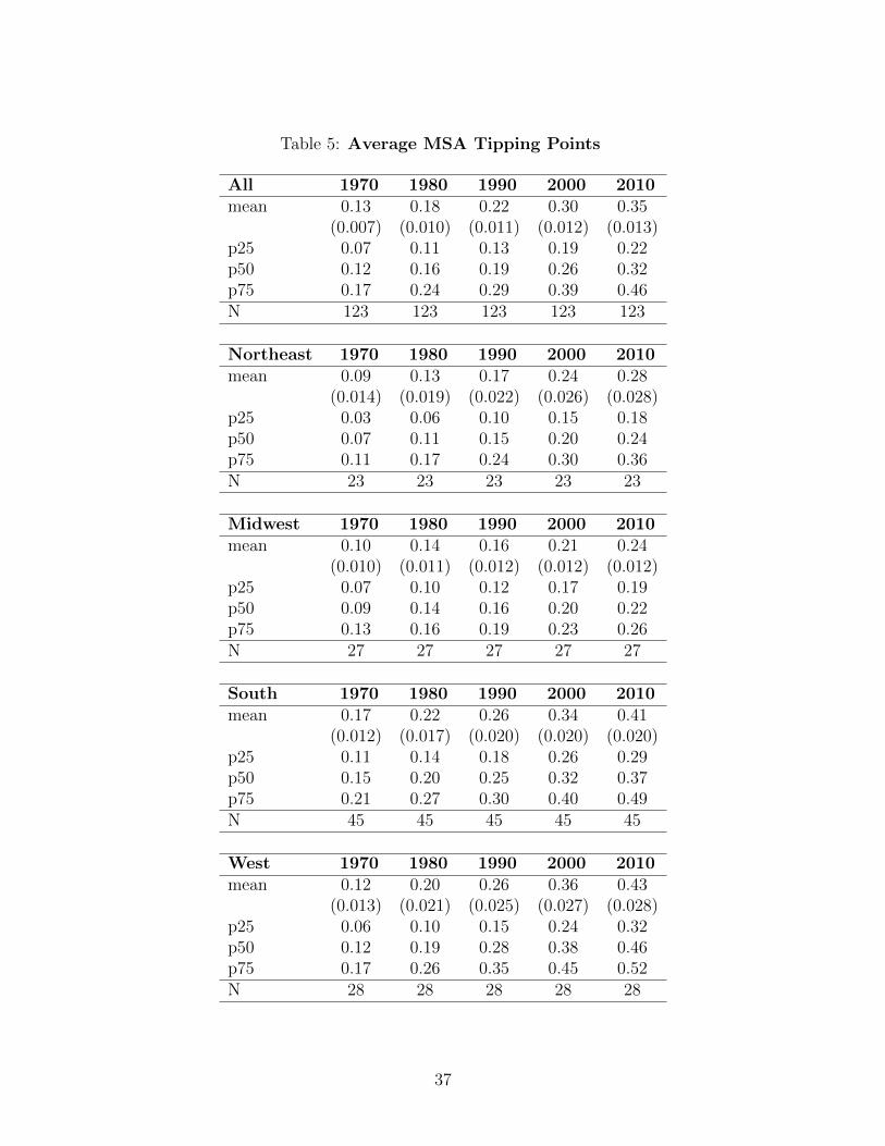
Table 5: Average MSA Tipping Points

All 1970 1980 1990 2000 2010mean 0.13 0.18 0.22 0.30 0.35

(0.007) (0.010) (0.011) (0.012) (0.013)p25 0.07 0.11 0.13 0.19 0.22p50 0.12 0.16 0.19 0.26 0.32p75 0.17 0.24 0.29 0.39 0.46N 123 123 123 123 123

Northeast 1970 1980 1990 2000 2010mean 0.09 0.13 0.17 0.24 0.28

(0.014) (0.019) (0.022) (0.026) (0.028)p25 0.03 0.06 0.10 0.15 0.18p50 0.07 0.11 0.15 0.20 0.24p75 0.11 0.17 0.24 0.30 0.36N 23 23 23 23 23

Midwest 1970 1980 1990 2000 2010mean 0.10 0.14 0.16 0.21 0.24

(0.010) (0.011) (0.012) (0.012) (0.012)p25 0.07 0.10 0.12 0.17 0.19p50 0.09 0.14 0.16 0.20 0.22p75 0.13 0.16 0.19 0.23 0.26N 27 27 27 27 27

South 1970 1980 1990 2000 2010mean 0.17 0.22 0.26 0.34 0.41

(0.012) (0.017) (0.020) (0.020) (0.020)p25 0.11 0.14 0.18 0.26 0.29p50 0.15 0.20 0.25 0.32 0.37p75 0.21 0.27 0.30 0.40 0.49N 45 45 45 45 45

West 1970 1980 1990 2000 2010mean 0.12 0.20 0.26 0.36 0.43

(0.013) (0.021) (0.025) (0.027) (0.028)p25 0.06 0.10 0.15 0.24 0.32p50 0.12 0.19 0.28 0.38 0.46p75 0.17 0.26 0.35 0.45 0.52N 28 28 28 28 28

37

Table 6: Median MSA Tipping Points

All 1970 1980 1990 2000 2010mean 0.11 0.16 0.21 0.28 0.33

(0.007) (0.010) (0.010) (0.013) (0.013)p25 0.06 0.10 0.12 0.17 0.22p50 0.10 0.13 0.17 0.24 0.31p75 0.16 0.22 0.27 0.37 0.43N 123 123 123 123 123

Northeast 1970 1980 1990 2000 2010mean 0.09 0.12 0.15 0.22 0.26

(0.013) (0.017) (0.019) (0.025) (0.025)p25 0.03 0.06 0.09 0.14 0.18p50 0.07 0.10 0.14 0.18 0.23p75 0.10 0.14 0.21 0.28 0.31N 23 23 23 23 23

Midwest 1970 1980 1990 2000 2010mean 0.09 0.12 0.14 0.19 0.22

(0.009) (0.009) (0.09) (0.010) (0.010)p25 0.06 0.09 0.11 0.17 0.18p50 0.08 0.12 0.14 0.17 0.22p75 0.11 0.14 0.16 0.21 0.24N 27 27 27 27 27

South 1970 1980 1990 2000 2010mean 0.14 0.20 0.25 0.32 0.38

(0.013) (0.017) (0.020) (0.022) (0.022)p25 0.09 0.13 0.17 0.24 0.30p50 0.11 0.17 0.22 0.29 0.35p75 0.19 0.24 0.29 0.37 0.43N 45 45 45 45 45

West 1970 1980 1990 2000 2010mean 0.11 0.19 0.25 0.36 0.42

(0.013) (0.021) (0.025) (0.027) (0.028)p25 0.05 0.10 0.14 0.24 0.31p50 0.12 0.17 0.26 0.38 0.43p75 0.17 0.25 0.34 0.44 0.53N 28 28 28 28 28

38

Table 7: Correlation in Mean MSA Tipping PointsYear 2010 2000 1990 1980 19702010 1.002000 0.88 1.001990 0.85 0.97 1.001980 0.81 0.93 0.98 1.001970 0.65 0.79 0.84 0.88 1.00# MSA 123 123 123 123 123

Table 8: Comparison of CMR and Revealed Preference Tipping Points

1990 1980 1970

% Marginal Tracts in MSA (below TP) 0.212 0.193 -0.015(0.069)** (0.067)** (0.055)

% Marginal Tracts in MSA (above TP) 0.311 0.121 0.603(0.169) (0.157) (0.123)**

Constant (Avg. Diff in CMR & RP MSA TP) -0.153 -0.102 -0.077(0.021)** (0.020)** (0.017)**

R2 0.17 0.12 0.26N 101 100 93

Table 9: Effect of Preferences and Options on Tipping Points

1970 1980 1990 2000 2010

Minority HHI -0.011 -0.034 -0.070 -0.097 -0.144(0.005)* (0.007)** (0.009)** (0.012)** (0.015)**

Non-minority HHI 0.006 0.026 0.055 0.066 0.112(0.005) (0.007)** (0.009)** (0.012)** (0.015)**

Race Prefs. 0.066 0.076 0.058 0.032 -0.005(0.007)** (0.012)** (0.012)** (0.011)** (0.008)

Constant 0.128 0.169 0.218 0.293 0.300(0.012)** (0.016)** (0.018)** (0.020)** (0.020)**

Region Fixed Effects Y Y Y Y Y

R2 0.55 0.52 0.57 0.55 0.58N 116 116 118 118 119

39

05

1015

Pro

b. D

ensi

ty

−.6 −.4 −.2 0 .2Tipping Difference

All Marginal Tracts

1970

05

1015

Pro

b. D

ensi

ty

−.6 −.4 −.2 0 .2Tipping Difference

All Marginal Tracts

1980

05

1015

Pro

b. D

ensi

ty

−.6 −.4 −.2 0 .2Tipping Difference

All Marginal Tracts

1990

Tipping Difference as Mean Tipping Point of Marginal Tracts

Figure 5: Kernel density plot of the difference between the CMR tipping points and meanMSA tipping points using all tracts, and using the marginal census tracts that are within 5percentage points of their tipping point.

40

05

1015

Pro

b. D

ensi

ty

−1 −.5 0 .5Tipping Difference

All Marginal Tracts

1970

05

1015

Pro

b. D

ensi

ty

−1 −.5 0 .5Tipping Difference

All Marginal Tracts

1980

05

1015

Pro

b. D

ensi

ty

−1 −.5 0 .5Tipping Difference

All Marginal Tracts

1990

Tipping Difference as Median Tipping Point of Marginal Tracts

Figure 6: Kernel density plot of the difference between the CMR tipping points and medianMSA tipping points using all tracts, and using just the marginal census tracts that are within5 percentage points of their tipping point.

41

−.2

−.1

0.1

.2E

ffect

of 1

std

. cha

nge

Minority HHI Non−minority HHI Race Prefs.

C1970 C1980C1990 C2000C2010

Effect of Preferences and Outside Option on Tipping Points

Figure 7: A plot of coefficient estimates from a regression of MSA tipping points on standard-ized measures of racial preferences and Herfindahl-Hirschman Indices (HHI) of the minorityand non-minority concentration of the MSA in census years C1970-C2010.

42