Working Paper Series · We start by showing that sticky price models imply that the documented...

Working Paper Series Estimating the optimal inflation target from trends in relative prices

Klaus Adam, Henning Weber

Disclaimer: This paper should not be reported as representing the views of the European Central Bank (ECB). The views expressed are those of the authors and do not necessarily reflect those of the ECB.

No 2370 / February 2020

Abstract

Using the official micro price data underlying the U.K. consumer price index, we document a

new stylized fact for the life-cycle behavior of consumer prices: relative to a narrowly defined set

of competing products, the price of individual products tends to fall over the product lifetime.

We show that this data feature has important implications for the optimal inflation target.

Constructing a sticky-price model featuring a product life cycle and heterogeneous relative-

price trends, we derive closed-form expressions for the optimal inflation target under Calvo and

menu-cost frictions. We show how the optimal target can be estimated from the observed trends

in relative prices. For the U.K. economy, we find the optimal target to be equal to 2.6% in 2016.

It has steadily increased over the period 1996 to 2016 due to changes in relative price trends

over this period.

Keywords: optimal inflation, micro price data, U.K. inflation target

JEL Class. No.: E31

ECB Working Paper Series No 2370 / February 2020 1

Non-technical Summary

A defining feature of modern economies is the high rate of product turnover in the market place. This

research paper shows that product turnover and the product life cycle are important for determining

the optimal inflation rate that a welfare maximizing central bank should target. Previous literature

on the design of monetary policy often abstracts from product turnover and its consequences.

We use the official micro price data that underlies the construction of the consumer price index in

the United Kingdom and document a new set of facts for how product prices evolve over the product

lifetime. We then derive monetary policy implications from these facts.

We start by documenting that for most expenditure items, the price of individual products declines

over the product lifetime, relative to the average price of products in the specific expenditure item.

Put differently, new products tend to be initially expensive and become cheaper over their lifetime in

relative terms. We then document considerable heterogeneity across expenditure items in the average

rate at which relative prices decline. Fashion and entertainment products, for instance, display very

high rates of relative price decline.

The set of empirical facts has strong normative implications for the optimal inflation target.

Specifically, we show that sticky price models imply that the documented relative price declines over

the product life reflects fundamental forces, such as the evolution of product quality or productivity

over time. This suggests that the documented relative price declines are efficient and that monetary

policy should choose its inflation target to facilitate the implementation of these trends.

We show that this can be achieved by setting a positive inflation target, where the optimal target

value is roughly equal to the average strength of the observed relative price decline across product

groups. For the U.K. economy the optimal inflation target is found to be significantly positive. It

stands at 2.6% for the year 2016, which is last year for which we observe micro price data. Over the

previous two decades, the optimal target has increased by around 1.2%. This is the case because

relative price trends have considerably accelerated over this period.


1 Introduction

A defining feature of modern economies is the high rate of product turnover in the market place.

This feature is documented in a number of micro studies (Nakamura and Steinsson (2008), Broda and

Weinstein (2010)) and is a key focus of the Schumpeterian literature on creative destruction (Aghion

and Howitt (1992)). It is, however, routinely abstracted from in the monetary policy literature. This

relative neglect of the product life cycle in the monetary literature is surprising, but not innocuous

from the perspective of monetary policy design: we show that features of the product life cycle turn

out to be important for determining the optimal inflation rate that a welfare maximizing central

bank should target.

We start our analysis by documenting a new set of stylized facts for the behavior of product prices

over the product lifetime. We do this by considering the official micro price data that underlies the

construction of the consumer price index in the United Kingdom. Our monthly data covers the years

1996-2016, features more than 1200 narrowly defined expenditure items and contains close to 29

million monthly price observations.

Using this data set, we document that for more than 90% of the expenditure items, the price of

individual products declines over the product lifetime, when measured relative to the average price

of products in the item.1 New products thus tend to be initially expensive, while becoming cheaper

over their lifetime in relative terms. There is also considerable heterogeneity in the average rate

of relative price decline across items. Items featuring some kind of ‘news value’, e.g., fashion and

entertainment products, display very high rates of price decline, while the vast majority of items

features rates of relative price decline between zero and five percent per year.

We also document that the downward trend in relative prices has significantly accelerated over the

past two decades. Expenditure items that dropped out of the consumption basket displayed smaller

relative price declines than the average expenditure item. Newly entering items displayed above

average relative price declines. Furthermore, within the set of continuing items, the expenditure

weights have shifted away from items displaying low rates of price decline towards items that display

stronger rates of price decline.

Taken together, these empirical facts have strong normative implications for the inflation target

that a welfare maximizing central bank should pursue. We arrive at this conclusion through a number

of steps.

We start by showing that sticky price models imply that the documented relative price declines

are actually efficient. This is the case because price rigidities and historically suboptimal rates of

inflation distort only the level of relative prices, but leave the age trend of relative prices unchanged.

As a result, the observed age trends of relative prices in the micro price data are identical to the ones

one would observe in a setting with perfectly flexible prices.

In light of this insight, the question of finding the optimal inflation rate is equivalent to determin-

1Relative prices can decline on average because there is constant product turnover. Absent turnover, this is hardly

possible.


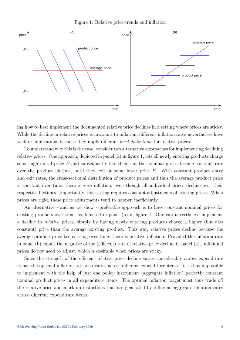
Figure 1: Relative price trends and inflation

time

price

average price

product price

(a)

time

price

average price

product price

(b)

ing how to best implement the documented relative price declines in a setting where prices are sticky.

While the decline in relative prices is invariant to inflation, different inflation rates nevertheless have

welfare implications because they imply different level distortions for relative prices.

To understand why this is the case, consider two alternative approaches for implementing declining

relative prices. One approach, depicted in panel (a) in figure 1, lets all newly entering products charge

some high initial price P and subsequently lets them cut the nominal price at some constant rate

over the product lifetime, until they exit at some lower price P . With constant product entry

and exit rates, the cross-sectional distribution of product prices and thus the average product price

is constant over time: there is zero inflation, even though all individual prices decline over their

respective lifetimes. Importantly, this setting requires constant adjustments of existing prices. When

prices are rigid, these price adjustments tend to happen inefficiently.

An alternative - and as we show - preferable approach is to have constant nominal prices for

existing products over time, as depicted in panel (b) in figure 1. One can nevertheless implement

a decline in relative prices, simply by having newly entering products charge a higher (but also

constant) price than the average existing product. This way, relative prices decline because the

average product price keeps rising over time: there is positive inflation. Provided the inflation rate

in panel (b) equals the negative of the (efficient) rate of relative price decline in panel (a), individual

prices do not need to adjust, which is desirable when prices are sticky.

Since the strength of the efficient relative price decline varies considerably across expenditure

items, the optimal inflation rate also varies across different expenditure items. It is thus impossible

to implement with the help of just one policy instrument (aggregate inflation) perfectly constant

nominal product prices in all expenditure items. The optimal inflation target must thus trade off

the relative-price and mark-up distortions that are generated by different aggregate inflation rates

across different expenditure items.


To determine how this trade-off is optimally resolved, we construct a sticky price model that

incorporates a product life cycle and rich forms of product heterogeneity. To obtain a model that

can capture key characteristics of micro price behavior, we augment the theoretical setup of Adam

and Weber (2019) by adding many heterogeneous expenditure items. The heterogeneity will imply

that the optimal target will generically fail to implement the efficient price distribution, unlike in

our earlier work.

Specifically, we introduce (i) heterogeneity in the productivity and product quality growth rates

across expenditure items, to be able to capture the observed heterogeneity in relative price trends;

(ii) heterogeneity in the degree of price rigidity and the rate of product turnover, to capture the

observed differences along these dimensions; and (iii) idiosyncratic components to product quality

and productivity, to capture the large and heterogeneous amounts of price dispersion in the data.

A second major difference relative to Adam and Weber (2019) is that the present paper not only

considers a setting with Calvo-type price-adjustment frictions, but also a setting with menu-cost

frictions that additionally features time-varying idiosyncratic productivity shocks.

Despite the richness of the model, we derive closed-form expressions for the optimal steady-state

inflation rate, i.e., for the inflation target that a welfare-maximizing central bank should adopt. This

is the case both for the setup with Calvo frictions and for the setup with menu-cost frictions.2

For Calvo frictions, we derive the optimal inflation target non-linearly and in closed-form. For

menu-cost frictions, we derive an analytic expression for the optimal target that is accurate to first

order. Reassuringly, however, the menu-cost result is identical to the one obtained when linearizing

the nonlinear Calvo result. Menu-cost and Calvo frictions thus deliver - to first-order accuracy -

identical optimal inflation targets.

To the best of our knowledge, we provide the first analytic result about optimal inflation in

a menu-cost setting.3 We thereby build on recent insights about the behavior of price distortions

derived in Alvarez et al. (2019). Since our setup essentially nests the menu-cost model of Golosov

and Lucas (2007) as a special case, it shows that the optimal inflation target is zero in a menu-cost

setting featuring only idiosyncratic productivity dynamics, but no systematic trends in productivity

or quality.

We then use our analytic first-order result, which is independent of the nature of price setting

frictions, to estimate the optimal inflation rate for the U.K. economy. We start by showing that to a

2Analytical aggregation is partly feasible because we abstain from explicitly modeling the product replacement

process, instead treat it as an exogenous (albeit heterogeneous) stochastic process. The precise economic forces

driving product replacement are not important for our results, as long as these forces are independent of the inflation

target pursued by the central bank. A number of potential forces naturally satisfy the independence requirement:

product replacement could be driven by changing consumer tastes that cause some products to fall out of fashion and

others to become fashionable; alternatively, replacement could be driven by negative productivity shocks that cause

the producer of an existing product to discontinue production and have the next best producer enter the market with

a new product.3Burstein and Hellwig (2008) numerically analyze the welfare costs of inflation in a menu-cost setting featuring cash

distortions. Blanco (2019) numerically analyzes a menu-cost setting featuring a lower bound constraint on nominal

interest rates.


first-order approximation, only three features of heterogeneity matter for the optimal inflation target:

(1) heterogeneity in productivity and quality growth across expenditure categories, which we show

to be identified by the estimated trends in relative prices; (2) heterogeneity in expenditure weights

across expenditure categories, and (3) heterogeneity in the steady-state real growth rates of (quality-

adjusted) output across expenditure categories. All remaining dimensions of heterogeneity, e.g., the

heterogeneity in Calvo price stickiness (Aoki (2001), Benigno (2004)), heterogeneity in product entry

and exit rates, heterogeneity in menu-costs or heterogeneity in idiosyncratic productivity shocks,

affect the optimal inflation target only to second-order.

The analytic first-order result has considerable empirical appeal, because it allows estimating the

optimal inflation target using micro price data only. We use the micro price data underlying the

construction of the UK CPI to estimate the optimal U.K. inflation target. For the year 2016, the

optimal target ranges between 2.6% and 3.2%, depending on how exactly one treats sales prices in the

data set. Independently of the treatment of sales prices, we robustly find that the optimal inflation

target has increased by around 1.2% over the period 1996 to 2016. This reflects the fact that negative

relative-price trends have become stronger over time through the introduction of new expenditure

items with stronger negative trends and the removal of items with less negative or positive trends.

The remainder of this paper is structured as follows. The next section presents the micro price

data set and a new set of stylized facts on relative price trends. Section 4 introduces a sticky price

model with Calvo frictions featuring a product life cycle and rich amounts of heterogeneity, which

allow capturing the documented heterogeneity in micro price data. Section 5 characterizes the steady

state outcome by aggregating the nonlinear model. Section 6 derives the nonlinear closed-form result

for the optimal inflation target. Section 7 considers the case with menu cost frictions. Section 8

explains how one can estimate the optimal inflation target from micro price data. Section 9 shows

that our estimation approach remains valid even if statistical agencies account only imperfectly for

quality progress. Section 10 presents our baseline estimation for the U.K. and section 11 offers various

robustness checks. A conclusion briefly summarizes. A series of appendices present our theoretical

aggregation result, various proofs and details of our empirical approach.

2 Related Literature

The model in the present paper is related to interesting quantitative work by Wolman (2011), who

considers a two sector sticky-price model where (goods and service) sectors feature different rates of

productivity growth. Using numerical methods, the optimal inflation target is shown to be slightly

negative for reasonable model calibrations.

Wolman (2011) abstracts from the product life cycle, which makes his setup a special case of the

one considered in the present paper. In fact, using the analytic expressions for the optimal inflation

target derived in the present paper and his model parameterization, we can replicate his numerical

findings.4 Our analytic expressions also reveal why the optimal inflation target remains fairly close

4Using proposition 1 derived below, we find the optimal inflation target to be -0.42% for his parametrization, while


to zero in his setting: in the absence of a product life cycle, remaining heterogeneity generates only

small (second-order) deviations from zero.

The literature discussing the role of the product life cycle in connection with monetary policy is

overall sparse and the present paper appears to be the first one drawing normative conclusions from

the product life cycle for monetary policy design.

The early product life cycle literature presented theoretical models of the evolution of firm entry,

exit and product innovation, but abstracted from nominal rigidities and monetary issues (Shleifer

(1986), Aghion and Howitt (1992), Klepper (1996)).

Nakamura and Steinsson (2008) present empirical evidence on product turnover in the BLS con-

sumer and producer price data sets. Broda and Weinstein (2010) present empirical evidence on

product creation and destruction for an important consumer good segment and quantify the quality

bias in consumer price indices. Bils (2009) decomposes aggregate price changes into changes origi-

nating from new products and changes from existing products, with the aim of improving estimated

quality growth. Aghion et al. (2019) also estimate the missing growth arising from incomplete adjust-

ments associated with the quality gains triggered by creative destruction. The issue of mismeasured

quality growth is orthogonal to the issue studied in this paper. In fact, as we show in section 9, our

results apply even when statistical agencies mismeasure quality growth and thus the inflation rate.

Argente, Lee and Moreira (2018) provide empirical evidence on how firms grow through the intro-

duction of new products and Argente and Yeh (2018) determine to what extent product replacement

and perpetual demand learning by firms contributes to monetary non-neutrality. To the best of our

knowledge, the latter paper is the only one incorporating a product life cycle into a setting with

nominal rigidities, but it does not study monetary policy implications.

The monetary policy literature has considered settings with endogenous firm entry and exit

(Bergin and Corsetti (2008), Bilbiie et al. (2008) and Bilbiie, Fujiwara and Ghironi (2014)), which

could be re-interpreted as models of endogenous product entry and exit.5 These papers study a

complementary setup in which monetary policy affects the entry decisions of firms/products, while

abstracting from firm/product heterogeneity. Product heterogeneity is, however, key to be able to

account for the observed relative price trends.

Also related is the optimal inflation literature, see Schmitt-Grohe and Uribe (2010) for an

overview. This literature has identified a number of complementary economic forces affecting the

optimal rate of inflation. Concerns about an occasionally binding lower bound constraint on nominal

interest rates, for instance, tend to generate a force towards positive inflation on average (Adam and

Billi (2006, 2007), Coibion, Gorodnichenko and Wieland (2012)). The same tends to be true when

wages are downwardly rigid (Carlsson and Westermark (2016), Benigno and Ricci (2011), Kim and

Ruge-Murcia (2009)). Conversely, the optimal inflation rate tends to become negative when taking

into account cash distortions (Khan, King and Wolman (2003)).

Wolman (2011) states that ”The optimal PCE inflation rate is approximately -0.4%” (p. 374).5Broda and Weinstein (2010) emphasize that product entry and exit dynamics differ considerably from firm or

establishment entry and exit dynamics.


3 U.K. Micro Price Data: New Evidence

We consider the micro price data that the Office of National Statistics (ONS) collects on a monthly

basis to compile the official consumer price index (CPI) for the United Kingdom (Office for National

Statistics (2014)). While the data has previously been analyzed in Bunn and Ellis (2012), Kryvtsov

and Vincent (2017), Blanco (2019) and Hahn and Marencak (2018), none of these papers considers

price trends over the product lifetime. More generally, it appears that the only other paper studying

life-cycle price trends is Melser and Syed (2016), who consider supermarket prices in Chicago. They

focus on trends in nominal prices and show that nominal prices of supermarket goods have a tendency

to fall over the product life, but that there is considerable heterogeneity across products, with many

goods’ prices actually increasing over the lifetime. We focus on life-cycle trends in relative prices and

find very consistent evidence of declining prices for a much broader set of goods and services. When

considering trends in nominal prices in our data set, we similarly find inconclusive evidence.

3.1 Data Description and Product Definition

We consider goods and service prices for the sample period February 1996 to December 2016. The

data covers the economic territory of the U.K., excluding offshore islands. For any given sales outlet,

data collectors find the most popular and regularly available products (or services), record price

information, as well as information for uniquely identifying the product and categorizing it into the

Classification of Individual Consumption by Purpose (COICOP). The raw data comprise almost 29

million individual price quotes, see table 1, and all prices are sampled on a monthly basis.

The publicly available micro price data set does not contain all price information underlying

the construction of the official CPI. For instance, it does not contain most of the housing related

expenditure components and also does not report so-called ‘centrally collected items’, such as ‘Golf

green fees’, ‘Horseracing admissions’ or ‘Air fares’. Despite this, the inflation rate obtained from

aggregating the price indices for which micro price data is available is very similar to the official CPI

inflation rate, see the top panel of figure 2.

Our analysis of relative price trends over the product life cycle requires us to track the same

product over time. Using the available product and outlet characteristics, we can construct around

736k unique product identifiers for the raw data. For confidentiality reasons, however, ONS does

not disclose all available location information. As a result, we have some product identifiers where

our data contains duplicate price quotes for the same month, so that we cannot perfectly distinguish

between products in these cases. We therefore discard all price quotes belonging to the identifiers

with duplicate price quotes. As table 1 shows, this leaves us with a slightly lower number of product

identifiers and about 24.5 million price quotes.

Following ONS practice, we also remove so-called ”invalid” price quotes, which are price quotes

that do not pass ONS cross-checking procedures (see Office for National Statistics (2014) for details).

Table 1 shows that removing duplicate and invalid price quotes leaves us with 22.8 million price

quotes.


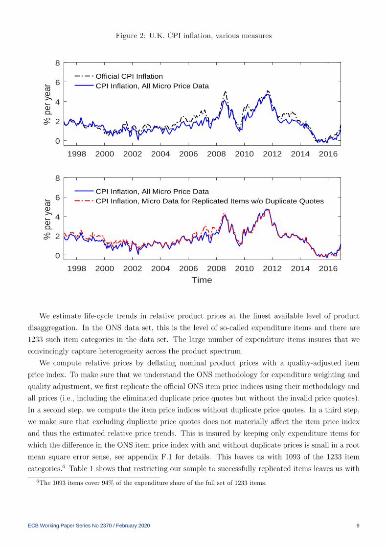
Figure 2: U.K. CPI inflation, various measures

1998 2000 2002 2004 2006 2008 2010 2012 2014 2016

0

2

4

6

8

% p

er y

ear

Official CPI InflationCPI Inflation, All Micro Price Data

1998 2000 2002 2004 2006 2008 2010 2012 2014 2016

Time

0

2

4

6

8

% p

er y

ear

CPI Inflation, All Micro Price DataCPI Inflation, Micro Data for Replicated Items w/o Duplicate Quotes

We estimate life-cycle trends in relative product prices at the finest available level of product

disaggregation. In the ONS data set, this is the level of so-called expenditure items and there are

1233 such item categories in the data set. The large number of expenditure items insures that we

convincingly capture heterogeneity across the product spectrum.

We compute relative prices by deflating nominal product prices with a quality-adjusted item

price index. To make sure that we understand the ONS methodology for expenditure weighting and

quality adjustment, we first replicate the official ONS item price indices using their methodology and

all prices (i.e., including the eliminated duplicate price quotes but without the invalid price quotes).

In a second step, we compute the item price indices without duplicate price quotes. In a third step,

we make sure that excluding duplicate price quotes does not materially affect the item price index

and thus the estimated relative price trends. This is insured by keeping only expenditure items for

which the difference in the ONS item price index with and without duplicate prices is small in a root

mean square error sense, see appendix F.1 for details. This leaves us with 1093 of the 1233 item

categories.6 Table 1 shows that restricting our sample to successfully replicated items leaves us with

6The 1093 items cover 94% of the expenditure share of the full set of 1233 items.


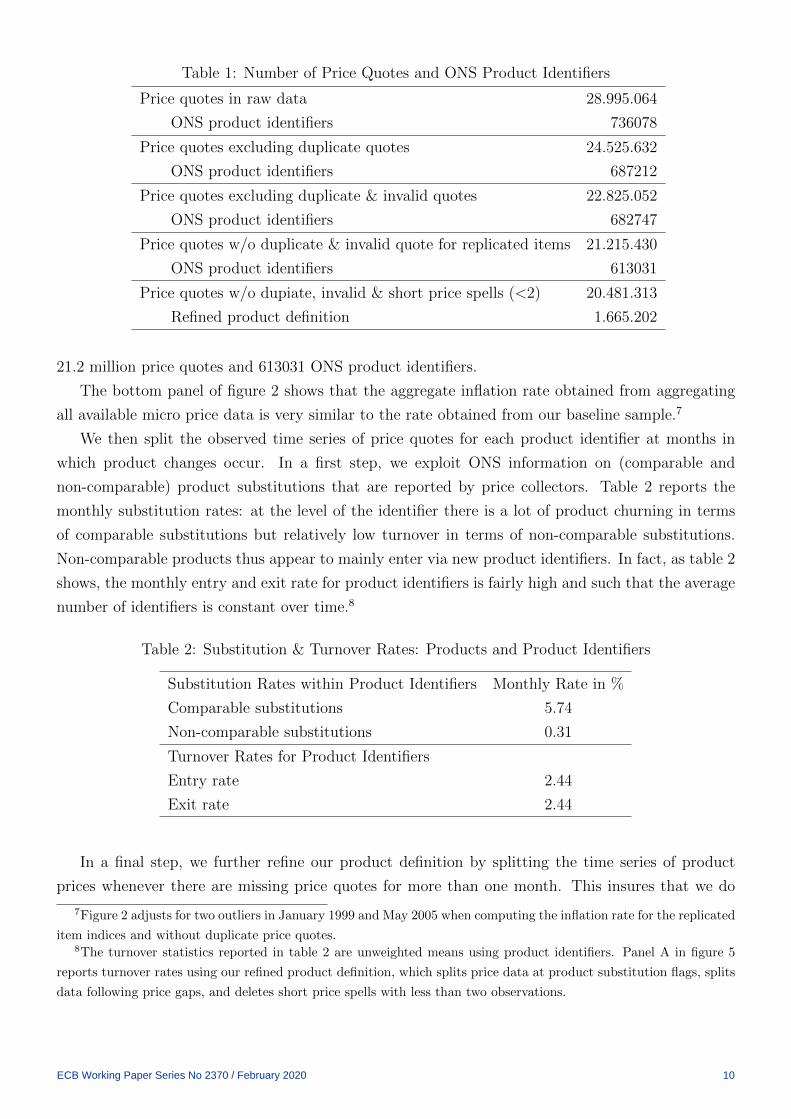
Table 1: Number of Price Quotes and ONS Product Identifiers

Price quotes in raw data 28.995.064

ONS product identifiers 736078

Price quotes excluding duplicate quotes 24.525.632


Price quotes excluding duplicate & invalid quotes 22.825.052


Price quotes w/o duplicate & invalid quote for replicated items 21.215.430


Price quotes w/o dupiate, invalid & short price spells (<2) 20.481.313

Refined product definition 1.665.202

21.2 million price quotes and 613031 ONS product identifiers.

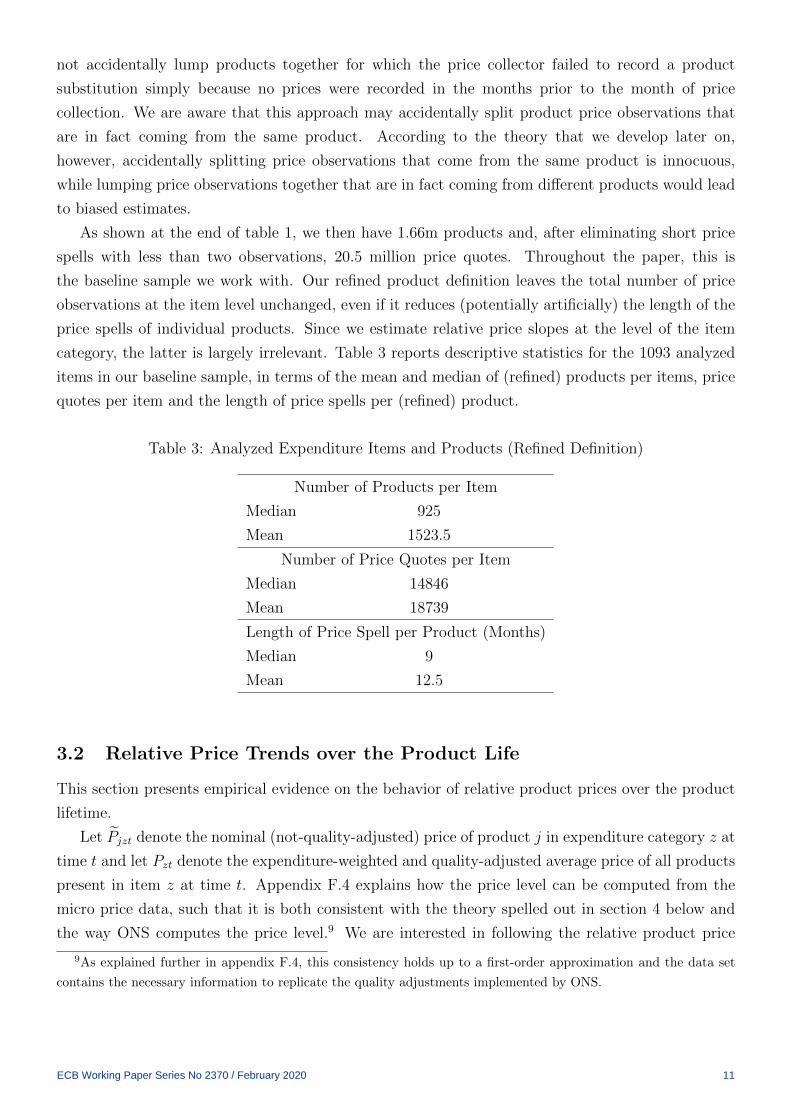
The bottom panel of figure 2 shows that the aggregate inflation rate obtained from aggregating

all available micro price data is very similar to the rate obtained from our baseline sample.7

We then split the observed time series of price quotes for each product identifier at months in

which product changes occur. In a first step, we exploit ONS information on (comparable and

non-comparable) product substitutions that are reported by price collectors. Table 2 reports the

monthly substitution rates: at the level of the identifier there is a lot of product churning in terms

of comparable substitutions but relatively low turnover in terms of non-comparable substitutions.

Non-comparable products thus appear to mainly enter via new product identifiers. In fact, as table 2

shows, the monthly entry and exit rate for product identifiers is fairly high and such that the average

number of identifiers is constant over time.8

Table 2: Substitution & Turnover Rates: Products and Product Identifiers

Substitution Rates within Product Identifiers Monthly Rate in %

Comparable substitutions 5.74

Non-comparable substitutions 0.31

Turnover Rates for Product Identifiers

Entry rate 2.44

Exit rate 2.44

In a final step, we further refine our product definition by splitting the time series of product

prices whenever there are missing price quotes for more than one month. This insures that we do

7Figure 2 adjusts for two outliers in January 1999 and May 2005 when computing the inflation rate for the replicated

item indices and without duplicate price quotes.8The turnover statistics reported in table 2 are unweighted means using product identifiers. Panel A in figure 5

reports turnover rates using our refined product definition, which splits price data at product substitution flags, splits

data following price gaps, and deletes short price spells with less than two observations.


not accidentally lump products together for which the price collector failed to record a product

substitution simply because no prices were recorded in the months prior to the month of price

collection. We are aware that this approach may accidentally split product price observations that

are in fact coming from the same product. According to the theory that we develop later on,

however, accidentally splitting price observations that come from the same product is innocuous,

while lumping price observations together that are in fact coming from different products would lead

to biased estimates.

As shown at the end of table 1, we then have 1.66m products and, after eliminating short price

spells with less than two observations, 20.5 million price quotes. Throughout the paper, this is

the baseline sample we work with. Our refined product definition leaves the total number of price

observations at the item level unchanged, even if it reduces (potentially artificially) the length of the

price spells of individual products. Since we estimate relative price slopes at the level of the item

category, the latter is largely irrelevant. Table 3 reports descriptive statistics for the 1093 analyzed

items in our baseline sample, in terms of the mean and median of (refined) products per items, price

quotes per item and the length of price spells per (refined) product.

Table 3: Analyzed Expenditure Items and Products (Refined Definition)

Number of Products per Item

Median 925

Mean 1523.5

Number of Price Quotes per Item

Median 14846

Mean 18739

Length of Price Spell per Product (Months)

Median 9

Mean 12.5

3.2 Relative Price Trends over the Product Life

This section presents empirical evidence on the behavior of relative product prices over the product

lifetime.

Let Pjzt denote the nominal (not-quality-adjusted) price of product j in expenditure category z at

time t and let Pzt denote the expenditure-weighted and quality-adjusted average price of all products

present in item z at time t. Appendix F.4 explains how the price level can be computed from the

micro price data, such that it is both consistent with the theory spelled out in section 4 below and

the way ONS computes the price level.9 We are interested in following the relative product price

9As explained further in appendix F.4, this consistency holds up to a first-order approximation and the data set

contains the necessary information to replicate the quality adjustments implemented by ONS.


Pjzt/Pzt over the lifetime of product j. To this end, we consider linear panel regressions of the form

lnPjztPzt

= fjz + ln (bz) · sjzt + ujzt, (1)

where fjz is a product and item-specific intercept term, sjzt the in-sample age of the product (nor-

malized to zero at the date of product entry), and ujzt a mean zero residual potentially displaying

serial and cross-sectional dependence. The coefficient of interest is the slope coefficient bz, which

measures the average growth rate of the relative product price over the product lifetime in item z.

Since regression (1) includes a product-specific intercept (fjz), the coefficient of interest (bz) remains

unaltered when using the quality-adjusted product price Pjzt instead of the non-adjusted price Pjzt in

the numerator on the left-hand side.10

If the set of products were constant over time, i.e., in the absence of product entry and exit, we

would have bz = 1, as not all products can simultaneously become cheaper or more expensive relative

to each other with product age.11 However, with product turnover, the price of each product relative

to the price of existing products can rise or fall over time because the existing set of products keeps

changing over time. This is the case, for instance, when products enter at a high price and leave at

a low price, in a way that the average price in the cross-section of products remains constant over

time. Each product’s relative price is then falling with product age.

We consider only linear trends in product age in equation (1) for two important reasons. First, we

observe only a censored measure of true product age: we see the in-sample age of a product but not

its true age. This distinction is relevant because products enter the ONS basket with a considerable

time delay, i.e., months or sometimes even years after their market introduction. The extent of

the time delay is also likely going to vary across products and items, which makes it impossible to

identify any non-linear age effects without observing the true product age. This said, Argente, Lee

and Moreira (2018) show - using scanner retail data for the United States, which allow observing

the precise time of product introduction - that prices decline at a rate that is very close to being

linear (see figure D.2 in their online appendix).12 Second, the linear specification will have a direct

structural interpretation that is relevant for determining the optimal inflation target in the sticky

price model that we introduce later on.

We estimate the slope coefficient bz by running the fixed-effect panel regression (1) for each

of the more than one thousand expenditure items in our baseline sample.13 Figure 3 displays the

10This is so because product quality is constant over the product lifetime, given our refined product definition. We

use the not-quality-adjusted price because this allows for some further interpretation of the intercepts fjz in the next

section.11For the case without product turnover, our theoretical model in fact predicts bz = 1.12Argente, Lee and Moreira (2018) show this to be robust to considering products with alternative durability or

product with alternative duration in the market, see their online appendices D.4 and D7.13We also estimated equation (1) using a random effects estimator. This delivers very similar results. Using a

first-difference specification, estimation results turn out to be less robust, especially with respect to the treatment of

sales prices. This is so because the first-difference estimator effectively estimates the slope bz using only the first and

last price observation of each product. These observations are with higher than average likelihood sales prices.


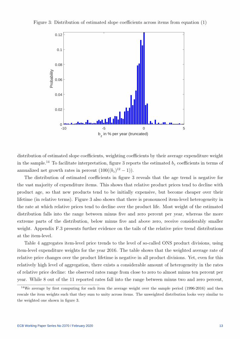
Figure 3: Distribution of estimated slope coefficients across items from equation (1)

-10 -5 0 5

bz in % per year (truncated)

0

0.02

0.04

0.06

0.08

0.1

0.12

Pro

babi

lity

distribution of estimated slope coefficients, weighting coefficients by their average expenditure weight

in the sample.14 To facilitate interpretation, figure 3 reports the estimated bz coefficients in terms of

annualized net growth rates in percent (100((bz)12 − 1)).

The distribution of estimated coefficients in figure 3 reveals that the age trend is negative for

the vast majority of expenditure items. This shows that relative product prices tend to decline with

product age, so that new products tend to be initially expensive, but become cheaper over their

lifetime (in relative terms). Figure 3 also shows that there is pronounced item-level heterogeneity in

the rate at which relative prices tend to decline over the product life. Most weight of the estimated

distribution falls into the range between minus five and zero percent per year, whereas the more

extreme parts of the distribution, below minus five and above zero, receive considerably smaller

weight. Appendix F.3 presents further evidence on the tails of the relative price trend distributions

at the item-level.

Table 4 aggregates item-level price trends to the level of so-called ONS product divisions, using

item-level expenditure weights for the year 2016. The table shows that the weighted average rate of

relative price changes over the product lifetime is negative in all product divisions. Yet, even for this

relatively high level of aggregation, there exists a considerable amount of heterogeneity in the rates

of relative price decline: the observed rates range from close to zero to almost minus ten percent per

year. While 8 out of the 11 reported rates fall into the range between minus two and zero percent,

14We average by first computing for each item the average weight over the sample period (1996-2016) and then

rescale the item weights such that they sum to unity across items. The unweighted distribution looks very similar to

the weighted one shown in figure 3.


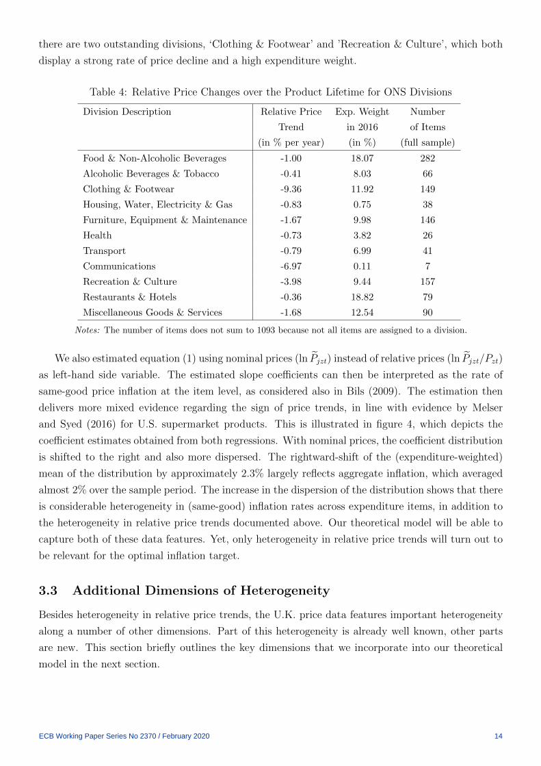
there are two outstanding divisions, ‘Clothing & Footwear’ and ’Recreation & Culture’, which both

display a strong rate of price decline and a high expenditure weight.

Table 4: Relative Price Changes over the Product Lifetime for ONS Divisions

Division Description Relative Price Exp. Weight Number

Trend in 2016 of Items

(in % per year) (in %) (full sample)

Food & Non-Alcoholic Beverages -1.00 18.07 282

Alcoholic Beverages & Tobacco -0.41 8.03 66

Clothing & Footwear -9.36 11.92 149

Housing, Water, Electricity & Gas -0.83 0.75 38

Furniture, Equipment & Maintenance -1.67 9.98 146

Health -0.73 3.82 26

Transport -0.79 6.99 41

Communications -6.97 0.11 7

Recreation & Culture -3.98 9.44 157

Restaurants & Hotels -0.36 18.82 79

Miscellaneous Goods & Services -1.68 12.54 90

Notes: The number of items does not sum to 1093 because not all items are assigned to a division.

We also estimated equation (1) using nominal prices (ln Pjzt) instead of relative prices (ln Pjzt/Pzt)

as left-hand side variable. The estimated slope coefficients can then be interpreted as the rate of

same-good price inflation at the item level, as considered also in Bils (2009). The estimation then

delivers more mixed evidence regarding the sign of price trends, in line with evidence by Melser

and Syed (2016) for U.S. supermarket products. This is illustrated in figure 4, which depicts the

coefficient estimates obtained from both regressions. With nominal prices, the coefficient distribution

is shifted to the right and also more dispersed. The rightward-shift of the (expenditure-weighted)

mean of the distribution by approximately 2.3% largely reflects aggregate inflation, which averaged

almost 2% over the sample period. The increase in the dispersion of the distribution shows that there

is considerable heterogeneity in (same-good) inflation rates across expenditure items, in addition to

the heterogeneity in relative price trends documented above. Our theoretical model will be able to

capture both of these data features. Yet, only heterogeneity in relative price trends will turn out to

be relevant for the optimal inflation target.

3.3 Additional Dimensions of Heterogeneity

Besides heterogeneity in relative price trends, the U.K. price data features important heterogeneity

along a number of other dimensions. Part of this heterogeneity is already well known, other parts

are new. This section briefly outlines the key dimensions that we incorporate into our theoretical

model in the next section.


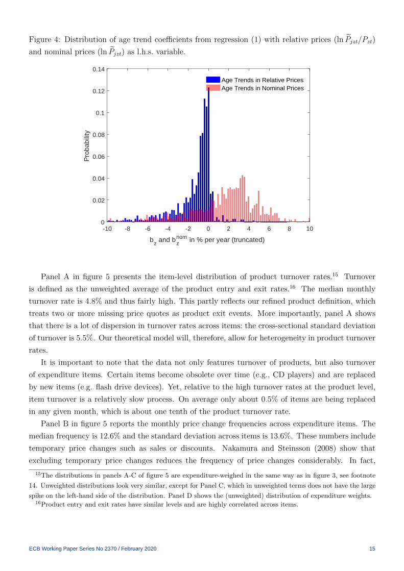
Figure 4: Distribution of age trend coefficients from regression (1) with relative prices (ln Pjzt/Pzt)

and nominal prices (ln Pjzt) as l.h.s. variable.

-10 -8 -6 -4 -2 0 2 4 6 8 10

bz and b

znom in % per year (truncated)

0

0.02

0.04

0.06

0.08

0.1

0.12

0.14

Pro

babi

lity

Age Trends in Relative PricesAge Trends in Nominal Prices

Panel A in figure 5 presents the item-level distribution of product turnover rates.15 Turnover

is defined as the unweighted average of the product entry and exit rates.16 The median monthly

turnover rate is 4.8% and thus fairly high. This partly reflects our refined product definition, which

treats two or more missing price quotes as product exit events. More importantly, panel A shows

that there is a lot of dispersion in turnover rates across items: the cross-sectional standard deviation

of turnover is 5.5%. Our theoretical model will, therefore, allow for heterogeneity in product turnover

rates.

It is important to note that the data not only features turnover of products, but also turnover

of expenditure items. Certain items become obsolete over time (e.g., CD players) and are replaced

by new items (e.g. flash drive devices). Yet, relative to the high turnover rates at the product level,

item turnover is a relatively slow process. On average only about 0.5% of items are being replaced

in any given month, which is about one tenth of the product turnover rate.

Panel B in figure 5 reports the monthly price change frequencies across expenditure items. The

median frequency is 12.6% and the standard deviation across items is 13.6%. These numbers include

temporary price changes such as sales or discounts. Nakamura and Steinsson (2008) show that

excluding temporary price changes reduces the frequency of price changes considerably. In fact,

15The distributions in panels A-C of figure 5 are expenditure-weighed in the same way as in figure 3, see footnote

14. Unweighted distributions look very similar, except for Panel C, which in unweighted terms does not have the large

spike on the left-hand side of the distribution. Panel D shows the (unweighted) distribution of expenditure weights.16Product entry and exit rates have similar levels and are highly correlated across items.


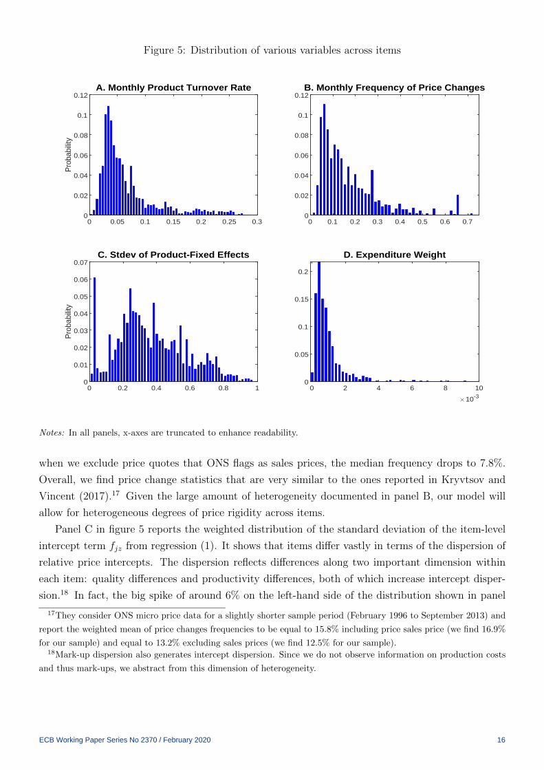
Figure 5: Distribution of various variables across items

A. Monthly Product Turnover Rate

0 0.05 0.1 0.15 0.2 0.25 0.30

0.02

0.04

0.06

0.08

0.1

0.12

Pro

babi

lity

B. Monthly Frequency of Price Changes

0 0.1 0.2 0.3 0.4 0.5 0.6 0.70

0.02

0.04

0.06

0.08

0.1

0.12

C. Stdev of Product-Fixed Effects

0 0.2 0.4 0.6 0.8 10

0.01

0.02

0.03

0.04

0.05

0.06

0.07

Pro

babi

lity

D. Expenditure Weight

0 2 4 6 8 10

10-3

0

0.05

0.1

0.15

0.2

Notes: In all panels, x-axes are truncated to enhance readability.

when we exclude price quotes that ONS flags as sales prices, the median frequency drops to 7.8%.

Overall, we find price change statistics that are very similar to the ones reported in Kryvtsov and

Vincent (2017).17 Given the large amount of heterogeneity documented in panel B, our model will

allow for heterogeneous degrees of price rigidity across items.

Panel C in figure 5 reports the weighted distribution of the standard deviation of the item-level

intercept term fjz from regression (1). It shows that items differ vastly in terms of the dispersion of

relative price intercepts. The dispersion reflects differences along two important dimension within

each item: quality differences and productivity differences, both of which increase intercept disper-

sion.18 In fact, the big spike of around 6% on the left-hand side of the distribution shown in panel

17They consider ONS micro price data for a slightly shorter sample period (February 1996 to September 2013) and

report the weighted mean of price changes frequencies to be equal to 15.8% including price sales price (we find 16.9%

for our sample) and equal to 13.2% excluding sales prices (we find 12.5% for our sample).18Mark-up dispersion also generates intercept dispersion. Since we do not observe information on production costs

and thus mark-ups, we abstract from this dimension of heterogeneity.


C is due to cigarettes (various types) and gasoline (petrol and diesel). Both of these items have a

high expenditure weight (around 3% each), but also - due to low degrees of quality and productivity

differences - very homogeneous prices. Overall, panel C reveals that for many items, intercept dis-

persion and thus productivity and/or quality dispersion is very large in the cross section of products.

In light of this finding, our model will allow for idiosyncratic productivity and quality differences

across products within each item.

Panel D in figure 5 displays the distribution of expenditure weights across items, which is the

distribution that has been used to compute the weighted distributions in the other panels of the figure.

Panel D shows that most items have an expenditure weight around one tenth of a percent, but that

there is a relatively long right tail to the distribution. To reflect this dimension of heterogeneity, our

model will allow for different expenditure weights across items, see the next section.

4 Sticky Price Model with a Product Life Cycle

This section introduces a sticky-price model featuring a product life cycle. We consider Calvo price

adjustment frictions in our baseline specification, as this will allow for a complete nonlinear aggrega-

tion and derivation of the optimal inflation rate. The case with menu-cost frictions will be discussed

in section 7.

The model contains a range of new elements that allow capturing the key dimensions of product

and price heterogeneity documented in section 3. In particular, it features multiple expenditure

items, each of which is populated by a continuum of heterogeneous products. Expenditure items

are allowed to have different degrees of price stickiness and different product-entry and exit rates.

The model also allows for heterogeneity in productivity and quality trends across items, which is key

for being able to capture the heterogeneity in relative price trends documented before. Finally, the

model allows for idiosyncratic elements in product quality and productivity, which allows capturing

the large and heterogeneous amounts of dispersion in relative prices observed in the data. The setup

in this section non-trivially generalizes the one studied in Adam and Weber (2019), which does not

feature heterogeneity along any of these dimensions.

The next sections present the model, derive the steady state of the economy and a closed-form

expression for the optimal steady-state inflation rate.

4.1 Demand Side and Production Side

The demand side of the model is standard and consists of a representative consumer with balanced-

growth consistent preferences over an aggregate consumption good Ct and hours worked Lt, described

by

E0

∞∑t=0

βt

([CtV (Lt)]

1−σ − 1

1− σ

), (2)


where β ∈ (0, 1) is a discount factor and σ > 0.19 The household faces the flow budget constraint

Ct +Kt+1 +Bt

Pt= (rt + 1− d)Kt +

WtLtPt

+Bt−1

Pt(1 + it−1)− Tt, (3)

where Kt+1 denotes the capital stock, Bt nominal government bond holdings, Pt the nominal price of

the aggregate consumption good, it−1 the nominal interest rate, Wt the nominal wage rate, rt the real

rental rate of capital, d the depreciation rate of capital, and Tt a summary variable that contains lump

sum taxes and firm profits, which the household takes as given. Household borrowing is subject to

a no-Ponzi scheme constraint. The first-order conditions characterizing optimal household behavior

are standard and derived in appendix A.1. To insure that utility remains bounded, we assume

β (γe)1−σ < 1,

where γe ≥ 1 denotes the steady-state growth rate of the aggregate economy under balanced growth,

as defined in equation (30) below.

The aggregate consumption good Ct is made up of Zt different consumption items (in the language

of the ONS). A consumption item is a product category, e.g., ”Flatscreen TV, 30-inch display” or

”CD-player, portable”, which itself contains a range of individual products. Letting Czt (z = 1, ..., Zt)

denote consumption of item z in period t, we have

Ct =Zt∏z=1

(Czt)ψzt , (4)

where ψzt ≥ 0 denotes the expenditure weight for item z at time t and∑Zt

z=1 ψzt = 1. We allow the

set of items Zt and the expenditure weights ψzt to be time-varying, so as to capture the fact that

ONS regularly drops and adds items to its consumption basket and adjusts the expenditure weights

over time.20

For simplicity, we interpret item entry and exit or changing expenditure weights for items as

being due to changing consumer tastes. Obviously, item substitution could be due to a variety of

other factors, such as increased competition from a different item, e.g., flash-drive devices becoming

increasingly competitive relative to portable CD players and thus leading to the exit of the latter.

We refrain from explicitly modeling competition across items, and instead take changes in the item

structure as exogenous. In the U.K. data, the item structure changes only slowly over time, with on

average 0.5% of items leaving the sample every month.

Every item contains a large number of differentiated products. To capture this fact, item level

consumption Czt is a Dixit-Stiglitz aggregate of individual products j ∈ [0, 1], so that

Czt =

(∫ 1

0

(QjztCjzt

) θ−1θ

dj

) θθ−1

, (5)

19We assume σ > 0 and that V (·) is such that period utility is strictly concave in (Ct, Lt) and that Inada conditions

are satisfied. We also assume that V (·) is such that the steady state amount of labor is positive.20We assume Zt to be a stationary stochastic process that assumes an integer value Z > 0 in the steady state.


where Cjzt denotes the consumed physical units of product j in item z in period t, Qjzt the quality

level of the product and θ > 1 the elasticity of substitution between products. We consider a

constant product variety over time, because our data does not offer any information about variety

trends.21 The aggregation assumes that consumption goods with higher product quality deliver

proportionately higher consumption services relative to consumption goods with a lower quality

level. This is a standard approach for modeling the quality content of goods, see Schmitt-Grohe and

Uribe (2012).

In equilibrium, the quantity of products Cjzt consumed must be equal to the quantity Yjzt pro-

duced, net of the quantity invested. Individual products are produced using a Cobb-Douglas pro-

duction function

Yjzt = AztGjzt (Kjzt)1− 1

φ (Ljzt)1φ , (6)

where Azt denotes the level of productivity common to all producers of products in item z and Gjzt a

product-specific productivity factor that captures idiosyncratic productivity components, as well as

productivity dynamics associated with experience accumulation in the manufacturing of the product.

The variables Kjzt and Ljzt, respectively, denote the capital and labor inputs into production.

In line with the evidence in micro price data, there will be constant churning of products j at

the level of each expenditure item z. In the U.K. data, product entry and exit is - unlike the entry

and exit of expenditure items - a fast moving process, see section 3.3. In practice, product turnover

may take place for a variety of reasons: (1) consumers may simply no longer demand a specific

product and demand other products instead, (2) the producers of a particular product may receive a

sufficiently negative productivity shock that causes the product to become uncompetitive and being

replaced by a new product, or (3) a newly available product is in quality-adjusted terms simply more

attractive. Whatever is the precise cause for product turnover, we assume that it can be described

by a product-specific, idiosyncratic and exogenous Poisson process with arrival rate δz ∈ (0, 1). We

thus assume that monetary policy does not affect the product turnover dynamics.

For simplicity, we assign to the newly entering product the same product index j as to the exiting

product. Let sjzt denote the age of product j in item z at time t, with sjzt = 0 in the period of

entry. Given this definition, the time t − sjzt denotes - at any period t - the date at which product

j entered into the economy.

We now describe how the productivity processes (Gjzt, Azt) and the quality process (Qjzt) evolve

over time. Product-specific productivity Gjzt is given by

Gjzt = Gjzt · εGjzt, (7)

where Gjzt denotes an experience-related productivity component for product j and εGjzt a idiosyn-

cratic product-specific productivity component. The latter is independently drawn at the time of

21The number of products sampled by ONS at the item level is not a function of true underlying product variety, but

instead governed by the desire to minimize measurement error. Product inclusion decisions thus reflect the variability

of underlying product prices and the item’s expenditure weight, see chapter 4 in ONS (2014).


product entry from some distribution ΞGz , that is

εGjzt ∼ ΞGz , (8)

with εGjzt > 0 and E[(εGjzt)θ−1] = 1, and remains constant over the lifetime of the product. We incor-

porate product-specific relative productivities (εGjzt), so that the model can replicate the standard-

deviation of product fixed effects, as well as its heterogeneity across items, as documented in figure

5.22 The experience-related productivity component Gjzt evolves over time according to

Gjzt =

1 for sjzt = 0,

gztGjzt−1 otherwise,(9)

with

gzt = gzεgzt, (10)

where gz ≥ 1 denotes the average growth rate of this productivity component and captures the

average rate of experience accumulation in the production of products in item z. The disturbance

εgzt is an arbitrary stationary process satisfying E ln εgzt = 0. Heterogeneity in the experience growth

rates gz allows the model to match different rates of relative price decline across items, as present in

figure 3.

The common item-level productivity Azt evolves according to

Azt = aztAzt−1

azt = azεazt,

where az ≥ 1 denotes the average productivity growth rate and εazt is an arbitrary stationary process

satisfying E ln εazt = 0. While accumulated experience Gjzt associated with product j in item z is lost

upon exit of the product, the growth rate in the common productivity level Azt allows for permanent

productivity gains in item z. Heterogeneity in the productivity growth rates az thus allows the model

to account for relative price trends across items, e.g., the decline of the price of products relative to

the price of services, as emphasized in Wolman (2011). The item-level growth trends az also allow to

generate a disconnect between item-level productivity growth, which is affected by az, and item-level

relative price trends, which remain unaffected by az.

It now remains to describe the process determining product quality (Qjzt). We assume that the

product-specific quality level Qjzt remains constant over the product lifetime, but that quality can

change upon product substitution.23 The quality level of product j entering in period t is given by

Qjzt = Qzt · εQjzt, (11)

22Since the standard deviation of product fixed effects in figure 5 may alternatively be generated by idiosyncratic

product-specific relative quality components, we shall also introduce such components in equation (11) below. We

do not want to take a stance on whether the observed dispersion of product fixed effects in figure 5 is generated by

product-specific quality or productivity.23In model and data, we interpret a new quality level of the same product as being a new product. Since we assign

the same index j to the exiting and newly entering product, Qjzt must have a time subscript.


where εQjzt captures an idiosyncratic product-specific relative quality component and Qzt a common

item-level quality component. The idiosyncratic component is an independent draw from some

distribution ΞQz , that is

εQjzt ∼ ΞQz ,

with εQjzt > 0 and E[(εQjzt)θ−1] = 1, and remains constant over time. The common quality component

evolves according to

Qzt = qztQzt−1 (12)

qzt = qzεqzt, (13)

where qz ≥ 1 denotes the average quality progress in item z and εqzt a random component of quality

growth, which is an arbitrary stationary process satisfying E ln εqzt = 0. Heterogeneity in average

quality growth (qz) allows the model to generate different rates of relative price increase over the

product lifetime.24 Figure 3 shows that a few items in fact display upward trends in relative prices.

Since the quality of a product remains constant over its lifetime, we have

Qjzt = Qjzt−sjzt for all (j, z, t) ,

where sjzt denotes the age of product j in item z at time t.

The previous setup deliberately abstracts from the presence of time-varying idiosyncratic shocks

at the product level. Adding such shocks comes at the cost of considerably complicating the analytical

derivation of the optimal inflation rate under Calvo frictions. We shall incorporate also time-varying

idiosyncratic shocks once we consider menu cost frictions in section 7.

Let Pjzt denote the price at which one unit of output Yjzt is sold at time t. The price Pjzt will

be set by the producer optimally subject to price-adjustment frictions. The quality-adjusted price of

the product is defined as

Pjzt =PjztQjzt

, (14)

and the quality-adjusted price level for item z as

Pzt =

∫ 1

0

(PjztQjzt

)1−θ

dj

11−θ

. (15)

Aggregation across items z delivers the quality-adjusted overall price level

Pt =∏Zt

z=1

(Pztψzt

)ψzt. (16)

24Increases in relative prices over the product life cannot be generated by experience productivity (gz ≥ 1). Expe-

rience accumulation can only cause relative prices to decrease over the product life. This does not rule out that any

observed relative price increase/decrease in the data reflects the combined effect of experience accumulation (gz) and

quality progress (qz) at the same time. Our model and the empirical analysis allow for this.


The optimal inflation rate will be defined in terms of this (perfectly) quality-adjusted price level, i.e.,

inflation is defined as

Πt =PtPt−1

. (17)

We show in section 9 that our results are robust to the presence of imperfect quality adjustment.

Optimal product demand by consumers and market clearing implies that product demand satisfies

Yjzt = Yzt

(PjztPzt

)−θ(18)

Yzt = ψzt

(PztPt

)−1

Yt (19)

where

Yjzt ≡ QjztYjzt (20)

denotes output in constant quality units.

4.2 Optimal Price Setting

We now consider the producers’ price setting problem. We assume that the price of a product can

be chosen freely at the time of product entry, but that price adjustments at the product level are

subsequently subject to Calvo-type adjustment frictions.

Let αz ∈ [0, 1) denote the time-invariant idiosyncratic probability that the price of some product j

in item z can not be adjusted in any given period.25 Since product quality is constant over the product

lifetime (new qualities are treated as new products), we let producers directly choose the quality-

adjusted product price Pjzt. Let Wt denote the nominal wage and rt the real rental rate of capital.

The factor input mix (Kjzt, Ljzt) is then chosen to minimize production costs KjztPtrt + LjztWt

subject to the constraint imposed by the production function (6).

From standard cost minimization follows, see appendix A.2, that the nominal marginal costs are

given by

MCt =

(Wt

1/φ

) 1φ(

Ptrt1− 1/φ

)1− 1φ

. (21)

We can then express the price-setting problem for product j in a price-adjustment period t as follows:

maxPjzt

Et

∞∑i=0

(αz(1− δz))iΩt,t+i

Pt+i

[(1 + τ)PjztYjzt+i −

MCt+iAzt+iQjzt+iGjzt+i

Yjzt+i

](22)

s.t. Yjzt+i = ψzt

(PjztPzt+i

)−θ (Pzt+iPt+i

)−1

Yt+i, (23)

where MCt+i/ (Azt+iQjzt+iGjzt+i) denotes the effective nominal marginal costs when productivity is

equal to Azt+iGjzt+i and product quality is equal to Qjzt, which is constant over the product lifetime.

25We abstract here from the possibility that firms can charge temporary prices or sales prices. We discuss this

feature in our robustness section 11.2.


The variable Ωt,t+i denotes the representative household’s discount factor between periods t and t+ i,

and τ denotes a sales subsidy (tax) if τ > 0 (τ < 0). We assume

−1 < τ ≤ 1/(θ − 1), (24)

so that the sales subsidy cannot be higher than what is required to eliminate the monopoly distortion

in the flexible price equilibrium.

The constraint (23) captures consumers’ optimal product demand, as implied by equations (18)-

(19). Appendix A.3 shows that the optimal price P ?jzt satisfies

P ?jzt

Pt

(QjztGjzt

Qzt

)=

(θ

θ − 1

1

1 + τ

)Nzt

Dzt

, (25)

where the item-level variables Nzt and Dzt are independent of the product index j and defined in

the appendix. The previous equation shows that the optimal relative reset price (P ?jzt/Pt) depends

only on item-level variables (Nzt/Dzt) and on how the firm’s productivity (AztQjztGjzt) relates to

the average productivity of newly entering products (AztQzt), where productivity is measured in

quality-adjusted terms. In appendix A.4 we use this insight to derive a recursive representation for

the evolution of the quality-adjusted item price level Pzt.

5 Characterizing the Steady State Outcome

This section presents the key equations determining the economy’s deterministic balanced growth

path equilibrium under Calvo frictions. We obtain these equations by aggregating the nonlinear

sticky price model in closed form and by detrending variables by their respective balanced growth

path trends. The derivations are quite involved and are performed in appendices A, B, C and D.

At the end of this section, we briefly explain how these equations are modified when considering

menu-cost frictions instead.

The equilibrium equations presented below are intuitively accessible and reveal how mark-up

distortions and relative price distortions across expenditure items move the economy away from its

first-best allocation. They also reveal how the aggregate inflation rate affects these distortions.

We start by defining the steady state as a situation without aggregate shocks and without item

turnover, in which idiosyncratic shocks continue to operate:

Definition 1 A steady state is a situation with a fixed set of items Zt = Z, constant expenditure

weights ψzt = ψz, no aggregate item-level disturbances (gzt = gz, qzt = qz, azt = az ), and a constant

(but potentially suboptimal) inflation rate Π. The following idiosyncratic shocks continue to operate

in the steady state: product entry and exit shocks, shocks to price adjustment opportunities, and

product-specific shocks to quality and productivity that realize at the time of product entry.

Appendix D shows how aggregate inflation Π, the detrended values of aggregate output y, con-


sumption c and capital k, and hours worked L satisfy the following four simple equations:26

y =

(ρ(Π)

∆e

)(k1− 1

φL1φ

)(26)

c

(−∂V (L)/∂L

V (L)

)=

1

µ(Π)

1

∆e

(k

L

)1− 1φ(

1

φ

)(27)

1

β (γe)−σ− 1 + d =

1

µ(Π)

1

∆e

(k

L

)− 1φ(

1− 1

φ

)(28)

y = c+ (γe − 1 + d)k. (29)

Equation (26) is the aggregate production function that determines output as a function of the

aggregate capital and labor inputs. The variable ∆e is a productivity parameter that captures the

efficient (and detrended) steady-state distribution of productivities and qualities across products and

item categories.27 The term ρ(Π) ≤ 1 captures the distortions that arise from inefficient relative

price distortions, as defined in detail below.28 The size of these distortions depends on the inflation

rate, except in the special case with flexible prices, where we have ρ(Π) = 1 for all Π.

Equation (27) equates the marginal rate of substitution between consumption and work on the

l.h.s. to the marginal rate of transformation on the r.h.s. of the equation. The latter is distorted by

the aggregate mark-up distortion µ(Π), as defined further below. The mark-up distortion depends

on the degree of monopolistic competition, the level of output subsidies/taxes and the inflation rate.

Again, in the special case with flexible prices, the mark-up distortion is independent of the inflation

rate.

Equation (28) determines the optimal capital-to-labor ratio: it equates the marginal product of

capital on the r.h.s., again adjusted for potential mark-up-distortions, to the sum of the steady-state

real interest rate (1/β (γe)−σ − 1) and the capital depreciation rate (d) on the l.h.s. The parameter

γe ≡Z∏z=1

(azqz)ψzφ ≥ 1 (30)

denotes the steady-state growth rate of quality-adjusted aggregate output y and affects (via con-

sumption growth) the steady-state real interest rate.

Finally, equation (29) is the resource constraint, which says that output is consumed and invested

to keep the capital stock constant in detrended terms.

The aggregate mark-up distortion µ(Π) is an expenditure-weighted average of the item-level

mark-up distortions µz(Π) and given by

µ(Π) =Z∏z=1

µz(Π)ψz , (31)

where the item-level distortions are given by

µz(Π) ≡(

1

1 + τ

θ

θ − 1

)Mz

(1− αz(1− δz)β(γe)1−σ[(γe/γez) Π]θ−1

1− αz(1− δz)β(γe)1−σ[(γe/γez) Π]θ(gz/qz)−1

), (32)

26The existence conditions for a steady state are discussed in appendix D.3.27See appendix B for a definition.28Price dispersion that reflects differences in productivity or product quality is efficient.


for all z = 1, . . . Z, with

Mz ≡(

1− αz(1− δz)[(γe/γez) Π]θ−1

1− αz(1− δz)(gz/qz)θ−1

) 1θ−1

,

and

γez ≡ (azqz)(γe)1− 1

φ .

The relative price distortion ρ(Π) is given by

(ρ(Π)µ(Π))−1 =Z∑z=1

ψz(µz(Π)ρz(Π))−1, (33)

where for all z = 1, . . . Z the item-level relative price distortions ρz(Π) are given by

ρz(Π)−1 = M θz

(1− αz(1− δz)(gz/qz)θ−1

1− αz(1− δz)[(γe/γez) Π]θ(gz/qz)−1

). (34)

As is easy to see, for the limiting case without price stickiness (αz → 0 for all z), we have

µ =

(1

1 + τ

θ

θ − 1

)ρ = 1,

independently of Π. This shows that the flexible price equilibrium is efficient, whenever the output

subsidy τ is such that it eliminates the monopoly distortion (τ = 1/(θ − 1), so that µ = 1). This

mirrors results of standard New Keynesian models that do not feature product heterogeneity and a

product life cycle.

For the general case with price stickiness and suboptimal output subsidies, there exists a trade-

off between reducing mark-up distortions and reducing relative price distortions. In particular,

the steady-state inflation rate that minimizes the mark-up distortion, i.e., moves 1/µ(Π) closest to

one, is generally different from the steady-state inflation rate that minimizes the effects of relative

price distortions, i.e., moves ρ(Π) closest to one. While this difference is quantitatively small for

fully calibrated versions of the model, the trade-off between minimizing mark-up and relative-price

distortion considerably complicates further analytical derivations. We shall thus consider a limiting

case in which mark-up distortions are proportional to relative price distortions:29

Lemma 1 Consider a steady state with a potentially suboptimal inflation rate Π. For the limiting

case β (γe)1−σ → 1, we have

µ(Π) =

(1

1 + τ

θ

θ − 1

)1

ρ(Π).

The proportionality between the mark-up distortion, µ(Π), and the inverse relative price distor-

tion, 1/ρ(Π), implies that both distortions are minimized by the same inflation rate.30 We derive the

distortion-minimizing optimal inflation rate in the subsequent section.

29See appendix E.1 for the proof of lemma 1.30Note that this holds true independently of the level of the output subsidy τ .


Equations (26)-(29), (31) and (33) similarly hold with menu-cost frictions, except that one has

to incorporate the aggregate resource loss from price-adjustment costs into equation (29). Further-

more, the item-level mark-up and relative-price distortions (µz, ρz) are now different functions of the

model parameters. It seems difficult, though, to derive non-linear closed-form expressions for these

distortions in the presence of menu costs.

6 Optimal Inflation Target with Calvo Frictions

We now present our main theoretical result about the optimal inflation target for the case with

Calvo frictions. The optimal target is defined as the inflation rate that maximizes steady state

utility.31 The next section presents the non-linear closed-form solution for the optimal target. The

subsequent section presents a first-order approximation, which is useful for estimating the optimal

inflation target from micro price data. We show in section 7 that the approximate result also holds

when price adjustment frictions take the form of menu costs.

6.1 Nonlinear Closed-Form Result

The following proposition states our main result:

Proposition 1 Consider an arbitrary output subsidy/tax satisfying (24) and the limit β(γe)1−σ → 1.

The welfare maximizing steady-state inflation rate Π? is given by

Π? =Z∑z=1

ωzγezγegzqz, (35)

where γez is the output growth rate of item z and γe the aggregate growth rate, with

γezγe

=azqz∏Z

z=1 (azqz)ψz.

The item weights ωz ≥ 0 are given by

ωz ≡ωz∑Zz=1 ωz

,

with

ωz ≡ψzθαz(1− δz)(γe/γez)θ(Π?)θ(qz/gz)

[1− αz(1− δz)(γe/γez)θ(Π?)θ(qz/gz)] [1− αz(1− δz)(γe/γez)θ−1(Π?)θ−1].

31The underlying idea is that economic shocks generate only temporary deviations of the optimal inflation rate from

its steady-state value, so that the average inflation rate that a welfare-maximizing central bank should target is in

fact the optimal steady-state inflation rate. This holds true to a first-order approximation in the aggregate shocks.

Nonlinear terms can cause the time average of the optimal stochastic inflation rate to differ from its steady-state value,

but such terms tend to be quantitatively small in sticky-price models, as long as the lower bound on nominal rates is

not binding.


The proof of the proposition is contained in appendix E.2. It shows that the steady-state amount

of labor (L) does not depend on the inflation target (Π), so that the target is optimally chosen to

maximize steady-state consumption. Consumption is shown to depend on the inflation target only

via the aggregate markup distortion (which is proportional to the relative-price distortion under

the maintained assumptions). The inflation rate minimizing the markup distortion and maximizing

consumption is the one stated in the proposition.

Equation (35) shows that the optimal inflation target is a doubly-weighted average of the item-

level terms gz/qz. To interpret this finding, we start by discussing the role of the item-level terms

gz/qz. Thereafter, we assess the role of the two weights ωz and γez/γe.

Items with gz > qz generate a force towards positive inflation (Π∗ > 1), while items with gz < qz

generate a force towards deflation (Π∗ < 1). To understand why this is the case, abstract for a

moment from quality progress (qz = 1) and suppose gz > 1. Productivity then increases with

the lifetime of the product, so that old products should become increasingly cheaper relative to

newly entering products. In the presence of price setting frictions, this relative price decline of old

products is best implemented by having new products charge higher prices, i.e., by positive amounts

of inflation, rather than by having old products continuously adjust prices downward. This is so

because price cuts cannot be synchronized across products due to Calvo frictions and thereby give

rise to inefficient price dispersion.32 Now consider the polar case without age-dependent productivity

(gz = 1) and positive quality progress (qz > 1). New products can then be produced at increasingly

higher quality, without having to use more inputs into their production. New products should thus

become cheaper (in quality-adjusted terms), relative to old products. Again, in the presence of price

setting frictions, this is best achieved by having new products charge lower prices, i.e., via deflation,

rather than by having old product increase prices.

The proof of the proposition implies that the item-level term gz/qz captures the value of the

inflation target that eliminates inefficient price dispersion in item z. To the extent that gz/qz varies

across items, the optimal inflation rate must thus trade-off between the distortions across different

items. The optimal resolution of this trade-off is captured by the item weights γez/γz and ωz.

The first set of weights, γez/γz, capture the (quality-adjusted) output growth in item z relative to

the growth rate of the aggregate economy. This leads to an overweighting of items with fast output

growth and an underweighting of items with slow growth.

The second set of weights, ωz, are nonlinear functions of item-level fundamentals, i.e., the expen-

diture weight ψz, the product turnover rate δz, the price stickiness αz, and the demand elasticity

θ. These weights also depend on the item-level terms qz/gz and on the optimal inflation rate Π∗

itself. Admittedly, the dependence on Π∗ makes it hard to interpret the item weights ωz. Yet, for

the special case where an item features no price stickiness (αz = 0), the optimal item weight is zero

(ωz = 0). This is in line with the insights provided in Aoki (2001). Similarly, with only a single

item (Z = 1) and thus no trade-off between items, all weights are equal to one, so that we obtain

Π? = g1/q1. This is the special case with a single relative price trend considered in Adam and Weber

32With menu cost frictions, continous price cuts would be equally undesirable because price adjustment is costly.


(2019).

6.2 An Operational Approximate Result

This section derives a first-order approximation to the nonlinear analytic expression for the optimal

inflation target in proposition 1. We do so because a fully-fledged estimation based on the nonlinear

result is challenging, as this would require empirically identifying a large range of structural param-

eters in a model-consistent way.33 In contrast, estimation based on the approximate result can be

implemented using readily available micro price data, as explained further in section 8. The approx-

imate result also turns out to be robust to assuming menu-cost frictions instead of Calvo frictions,

see section 7.

Lemma 2 Consider an arbitrary output subsidy/tax satisfying (24) and the limit β(γe)1−σ → 1.

The optimal steady-state inflation rate is equal to

Π? =Z∑z=1

ψzγezγegzqz

+O(2), (36)

where O(2) denotes a second-order approximation error and where the approximation to equation

(35) has been taken around a point, in which gzqz

γezγe

and αz(1− δz)(γe/γez)θ−1 are constant across item

categories z = 1, . . . Z, but can vary to first order across items z.

The lemma shows - somewhat surprisingly - that only three dimensions of heterogeneity matter

for the inflation target to first order: heterogeneity in the expenditure weights ψz, heterogeneity in

the relative growth rates γez/γe and heterogeneity in the item-level terms gz/qz. Before explaining

how these three objects can be estimated from micro price data, the next section shows that the

same result applies with menu costs.

7 Optimal Inflation Target with Menu Costs

We now consider the optimal steady-state inflation target in a setting where price-adjustment frictions

take the form of menu costs and where producers are also subject to idiosyncratic productivity shocks.

We derive conditions under which the same inflation target as in lemma 2 is optimal in this setting.

The demand side of the economy is unchanged relative to our setting with Calvo frictions, but

the economy now evolves in continuous time. As before, common item-level productivity evolves

according to

d lnAzt = (ln az) dt

33For instance, using empirical price adjustment frequencies to estimate the price rigidity parameters αz, as is

commonly done in the literature, requires assuming that marginal production costs are not constant. The estimation

approach we adopt below does not rely on this assumption.


and experience productivity evolves according to

d lnGjzt = (ln gz) dt + σzdWjzt,

where σz > 0 captures the presence of product-specific idiosyncratic changes in productivity and

Wjzt denotes a standard Brownian motion. Such kind of shocks have not been present in the Calvo

setting considered before. The initial quality level Qjzt−sjzt and the initial experience level Gjzt−sjzt

are again drawn at the time of product entry, and average quality evolves according to

d lnQzt = (ln qz) dt.

Consider a product j in item z entering at time t. Maximization of real profits requires choosing

the initial product price Pjzt, which can be chosen at no cost, the stopping times τ ijz at which prices

are adjusted subsequently, and the associated price changes ∆Pjz(τijz), so as to

maxPjzt,τ ijz ,∆Pjz(τ ijz)∞i=1

E

∫ ∞t

e−r(1−δz)t

((1 + τ z)

PjztPt− MCt/PtAztQjztGjzt

)Yjztdt (37)

−∞∑i=1

e−r(1−δz)τ ijzκzdejzt(τ

ijz),

subject to the demand function (23), where Pjzt = Pjzt +∑

τ ijz<t∆Pjz(τ

ijz), r = − ln(β(γe)1−σ) ≥ 0

and where the price-adjustment cost parameter κz multiplies the efficient flex-price equilibrium real

profit dejzt(τijz) at adjustment time τ i.34

Following Alvarez et al. (2019), we assume that the firm’s profit function is sufficiently well

approximated by a quadratic expansion in the price gap, where the gap is defined as the difference

between firms’ relative price and the profit-maximizing relative price.35 Likewise, we assume that the

steady-state distribution of price gaps and the rate of price changes is differentiable with respect to

inflation.36 Taken together, these assumptions insure that the we can build on the insights provided

in proposition 1 in Alvarez et al. (2019).

An important difference between Calvo and menu-cost frictions is that the latter generate resource

costs when prices are adjusted. Let Fm(κz, λzZz=1) denote the aggregate adjustment costs when

the steady-state rate of price adjustment in item z is λz. Since λz depends on the aggregate inflation

rate, the minimization of aggregate adjustment costs introduces a new trade-off into the choice of

the optimal inflation rate. As we show below, this additional trade-off will not affect the optimal

inflation rate if one of the following conditions is satisfied:

Assumption 1 Suppose (κz, σ2z, δz) = (κ, σ2, δ) +O(1) and either

(i) menu costs are small (κ ∼ O(1)), or

34We choose this adjustment-cost specification to insure that dejzt depends neither on equilibrium inflation nor on

output subsidies, so that aggregate adjustment costs respond to inflation exclusively via the rate of price adjustment.35Technically, this requires the gaps to be of first order, which is the case whenever the adjustment bounds are of

first order. Results in Dixit (1991) suggest the latter to be the case when(σ2zκz)1/4 ∼ O(1).

36A necessary condition for this to be the case is that σz > 0, as assumed.


(ii) menu costs are large (κ ∼ O(0)), but

∂Fm(κz, λzZz=1)

∂λz· ∂2λz

(∂ ln Π)2

∣∣∣∣Π=

gzγez

qzγz

∝ ψz for all z = 1, ..., Z, (38)

where O(i) denotes terms of order i = 0, 1.

The next proposition shows how the insights from the Calvo model then extend to a menu-cost

setup:

Proposition 2 Consider a menu-cost setup where κz, σ2z, δ

2zZz=1 satisfy assumption 1 and output

subsidies τ z are such that item-level markup distortions µz are proportional to item-level relative price

distortions 1/ρz. The optimal steady-state inflation rate is then equal to

Π? =Z∑z=1

ψzγezγegzqz

+O(2), (39)

where O(2) denotes a second-order approximation error and where the approximation has been taken

around a point at which gzqz

γezγe

is constant across item categories z = 1, . . . , Z and where (κz, σ2z, δz) =

(κ, σ2, δ).

The proof of the proposition leverages insights about the symmetry of the price-gap distribution

derived in Alvarez et al. (2019) and can be found in appendix E.4. To the best of our knowledge,

proposition 2 is the first closed-form result about optimal inflation in a menu-cost setting. In the

special case with a single expenditure item (Z = 1) and without systematic quality and productivity

trends (g/q = 1), the model reduces to a setting that is very similar to the one studied in Golosov

and Lucas (2007).37 In this special case, the optimal inflation target involves zero inflation (Π? = 1).

Interestingly, the optimal inflation rate under menu costs is - to first order - the same as with

Calvo frictions. The proof of the proposition shows that this holds true because item-level price

distortions all react (to second-order accuracy at the point of approximation) in the same way to

deviations of inflation from its item-level optimal rate. This is so despite the presence of first-order

heterogeneity in the parameters κz, σ2z, δ

2zZz=1. The menu-cost model shares this property with the

Calvo model, which causes price dispersion to be minimized in both settings by the same inflation

rate.38

Assumption 1 insures that menu costs are either too small to matter for optimal inflation to first

order (condition (i)) or that they generate the same trade-off across items as the one generated by

price dispersion (condition (ii)). In particular, proportionality condition (38) requires the resource

loss associated with deviations from the item-level optimal inflation rate to be proportional to the

37Golosov and Lucas (2007) consider an idiosyncratic productivity process that is continously mean reverting. In

our setting, mean-reversion occurs in a Poisson-like fashion via product substitution.

38Recall that effective price stickiness in the Calvo model, αz(1−δz)(γe

γez

)θ−1

, can also differ to first order in lemma

2.


expenditure weight of the item.39 Minimizing price dispersion is then equivalent to minimizing the

resource loss from price adjustment costs.

Finally, the proportionality between mark-up and relative price distortions implies that both are

minimized by the same inflation rate. Under Calvo frictions, this proportionality was insured by the

limiting condition β(γe)1−σ → 1, see lemma 1. Under menu-cost frictions, this limiting condition

fails to guarantee proportionality, due to the presence of time-varying idiosyncratic shocks.40 This

requires imposing appropriate output subsidies, which then allows considering more general discount

factors.

Overall, it is quite reassuring so see that Calvo and menu-cost frictions deliver the same approx-

imate expression for the optimal inflation target. This is true even though the costs of deviating

from the optimal inflation target are typically quite different across the two frictions (Burstein and

Hellwig (2008)). Moreover, both frictions likely deliver different results for optimal inflation when

also considering higher-order terms.

8 Estimating the Optimal Inflation Target

The results about the optimal inflation target in lemma 2 and proposition 2 show that three dimen-

sions of heterogeneity matter to first order: heterogeneity in expenditure weights ψz, heterogeneity

in growth rates γez/γeand heterogeneity in the item-level terms gz/qz.

The first two dimensions can be readily identified from official micro price data sets. In particular,

the expenditure weights are naturally part of micro price data sets that are used to compute an

aggregate price index. The heterogeneity in growth rates can be identified using the model-implied

relationship γez/γe = Π/Πz, which allows using the sample means of Π and Πz to estimate γez/γ

e.

It thus only remains to identify item-level terms gz/qz. We first discuss how this can be achieved

in a Calvo setting, and thereafter discuss menu-cost settings. In fact, a main contribution of the paper

is to derive a model-consistent estimation approach that directly yields estimates of the item-level

terms gz/qz under fairly general conditions:41

Proposition 3 Consider a stochastic sticky price economy with Calvo frictions and with a stationary

(and potentially suboptimal) inflation rate Πt. Let T ?jz denote the set of periods in which the price of

product j in item z can be adjusted and let sjzt denote the product age. The optimal reset price P ?jzt

in adjustment periods, defined in equation (25), satisfies

lnP ?jzt

Pzt= f ?jz − ln

(gzqz

)· sjzt + u?jzt, for all t ∈ T ?jz, (40)

where the residual satisfies E[u?jzt] = 0.

39Since ∂λz/∂ ln Π|Πz=gzγez/qzγz

= 0, deviations of inflation from its optimal item-level rate produce no first-order

resource costs.40Inverse proportionality would similarly fail in a Calvo setup featuring time-varying idiosyncratic shocks.41See appendix E.5 for the proof.


The proposition shows that the optimal Calvo reset price displays an age trend at the rate gz/qz,

which is our parameter of interest. The result applies, whenever there is a strictly positive rate of

product turnover (δz > 0), as assumed, but is otherwise independent of the turnover rate. For the

case without item turnover (δz = 0), the model implies that the age trend is discontinuously different

and equal to zero.42

It may appear surprising that the age-trend coefficient in equation (40) reveals our parameter

of interest in a setting with sticky prices and potentially suboptimal inflation rates. To understand

why this is the case, we note that with flexible prices (αz = 0), the same relative price trend would

emerge. Specifically, the proof of proposition 3 implies that flexible prices satisfy

lnP fjzt

Pzt= f fjz − ln

(gzqz

)· sjzt + ufjzt, (41)

for all periods t in which the product is on offer. Price stickiness and suboptimal inflation rates thus

only affect the level of relative reset prices, i.e., the intercept term f ?jz and the residual u?jzt, but

leave the time trend of relative prices invariant. This invariance property is key for the ability to

identify the structural parameters gz/qz under Calvo frictions. In fact, it implies that the relative

price trends that are present in micro price data are efficient, i.e., reflect economic fundamentals.

This invariance property of relative price trends is by no means special to the Calvo setting. It

holds similarly if price adjustments are subject to menu cost frictions instead. Since menu costs

generate inaction bands around the frictionless optimal relative price, the optimal reset price under

menu cost frictions must display the same time trend as the frictionless price.

Equation (40) thus provides a highly tractable approach for empirically identifying gz/qz inde-

pendently of the source of price rigidities.43’44 Since product prices are reset only infrequently in

adjustment periods but stay constant otherwise, the entire price path of a product displays the very

same time trend as the reset prices. We thus have that the entire price path satisfies

lnPjztPzt

= fjz − ln

(gzqz

)· sjzt + ujzt, (42)

for some alternative intercept term and a residual that again satisfies E[ujzt] = 0.45 In our empirical

42This seeming discontinuity at δz = 0 arises only because steady state considerations also involve taking a limit, so

that one effectively considers a double limit: the limit δz → 0 and additionally the limit distribution for steady state

productivities implied by δz.43This is true even though the residual u?jzt can potentially contain a unit root, see the proof of proposition 3. Since

product lives tend to be short, the asymptotics of interest are the ones where the number of products gets large,

not the ones where the lifetime of the products get large. Non-stationarity is thus not an issue for consistency and

asymptotic normality of our estimates.44This is the case, despite the fact that the true product age sjzt is typically not observed. As is easily seen, using

the number of months since the product has been included into the price data set as the ‘age’ regressor, instead of the

true product age, affects only the estimated intercept term, but leaves the coefficient of interest multiplying the ‘age’

term unchanged. One can thus estimate the parameter of interest even without observing true product age.45Appendix E.6 derives the intercept term and the properties of the modified residual in the previous equation for

the case with Calvo frictions.


approach, we shall use equation (42) as our baseline equation, which uses all price observations. We

will consider estimates based on the reset prices only, see equation (40), in a robustness exercise.

Regression (42) is almost the one we have estimated in our empirical section 3. The only differ-

ences are that in section 3 we used the non-quality adjusted relative product price (ln(Pjzt/Pzt)) on

the left-hand side of equation (1) and that there was a different sign for the regression coefficient.

With product quality being constant across the product lifetime, the first difference does not affect

the estimated age coefficient, as it gets absorbed in the estimated constant; the second difference

only implies a trivial sign inversion. The estimates of slope coefficients bz displayed in figure 3 thus

already reveal the (negative) of the optimal item-level inflation rates.

9 Imperfect Quality Adjustment

The estimation approach and the underlying theory developed in the previous sections assume that

statistical agencies perfectly adjust prices for quality. This is clearly an idealized assumption, as a

number of studies show that quality adjustment is far from perfect (Bils (2009), Broda and Weinstein

(2010), Aghion et al. (2019)).

This section shows that failure to perfectly adjust prices for quality generates biases in the slope

coefficients identified in regression (40), i.e., the coefficient in front of the age trend will then not be

equal to ln gz/qz, unlike in the case with perfect quality adjustment. This is the case because the item

price level Pzt showing up on the left-hand side of the regression equation displays a different trend

when quality adjustment is imperfect. While this may be a source of concern, we show below that

the optimal inflation target computed according to lemma 2 based on these biased slope estimates

nevertheless delivers the welfare maximizing target for the imperfectly quality-adjusted price index.

In other words, the approach developed in the previous sections works perfectly well, even if quality

adjustment is imperfect, as is likely the case in practice.

To make this point most forcefully, we consider an extreme setting in which the statistical agency

makes no quality adjustments whatsoever. The item price level is thus computed using not-quality-

adjusted prices Pjzt and given by

Pzt ≡(∫ 1

0

(Pjzt)1−θdj

) 11−θ

, (43)

with the associated item-level inflation rate given by

Πzt = Pzt/Pzt−1.

Appendix E.7 derives the recursive law of motion for the not-quality adjusted item price level and

shows that in steady state the following holds:

Πz = qzΠz. (44)

The item-level inflation rate without quality adjustment Πz thus exceeds the quality-adjusted infla-

tion rate whenever there is quality growth (qz > 1). Similarly, the aggregate steady-state inflation


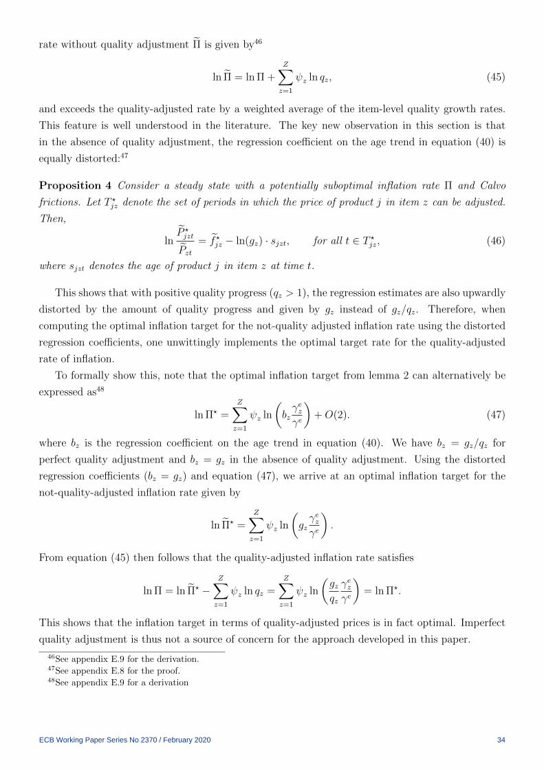
rate without quality adjustment Π is given by46

ln Π = ln Π +Z∑z=1

ψz ln qz, (45)

and exceeds the quality-adjusted rate by a weighted average of the item-level quality growth rates.

This feature is well understood in the literature. The key new observation in this section is that

in the absence of quality adjustment, the regression coefficient on the age trend in equation (40) is

equally distorted:47

Proposition 4 Consider a steady state with a potentially suboptimal inflation rate Π and Calvo

frictions. Let T ?jz denote the set of periods in which the price of product j in item z can be adjusted.

Then,

lnP ?jzt

Pzt= f ?jz − ln(gz) · sjzt, for all t ∈ T ?jz, (46)

where sjzt denotes the age of product j in item z at time t.

This shows that with positive quality progress (qz > 1), the regression estimates are also upwardly

distorted by the amount of quality progress and given by gz instead of gz/qz. Therefore, when

computing the optimal inflation target for the not-quality adjusted inflation rate using the distorted

regression coefficients, one unwittingly implements the optimal target rate for the quality-adjusted

rate of inflation.

To formally show this, note that the optimal inflation target from lemma 2 can alternatively be

expressed as48

ln Π? =Z∑z=1

ψz ln

(bzγezγe

)+O(2). (47)

where bz is the regression coefficient on the age trend in equation (40). We have bz = gz/qz for

perfect quality adjustment and bz = gz in the absence of quality adjustment. Using the distorted

regression coefficients (bz = gz) and equation (47), we arrive at an optimal inflation target for the

not-quality-adjusted inflation rate given by

ln Π? =Z∑z=1

ψz ln

(gzγezγe

).

From equation (45) then follows that the quality-adjusted inflation rate satisfies

ln Π = ln Π? −Z∑z=1

ψz ln qz =Z∑z=1

ψz ln

(gzqz

γezγe

)= ln Π?.

This shows that the inflation target in terms of quality-adjusted prices is in fact optimal. Imperfect

quality adjustment is thus not a source of concern for the approach developed in this paper.

46See appendix E.9 for the derivation.47See appendix E.8 for the proof.48See appendix E.9 for a derivation


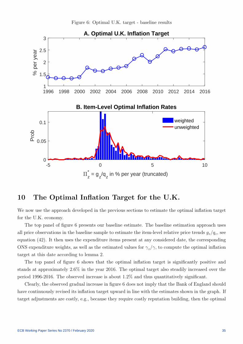
Figure 6: Optimal U.K. target - baseline results

1996 1998 2000 2002 2004 2006 2008 2010 2012 2014 20161

1.5

2

2.5

3%

per

yea

rA. Optimal U.K. Inflation Target

B. Item-Level Optimal Inflation Rates

-5 0 5 10

z* = g

z/q

z in % per year (truncated)

0

0.05

0.1

Pro

b

weightedunweighted

10 The Optimal Inflation Target for the U.K.

We now use the approach developed in the previous sections to estimate the optimal inflation target

for the U.K. economy.

The top panel of figure 6 presents our baseline estimate. The baseline estimation approach uses

all price observations in the baseline sample to estimate the item-level relative price trends gz/qz, see

equation (42). It then uses the expenditure items present at any considered date, the corresponding

ONS expenditure weights, as well as the estimated values for γz/γ, to compute the optimal inflation

target at this date according to lemma 2.

The top panel of figure 6 shows that the optimal inflation target is significantly positive and

stands at approximately 2.6% in the year 2016. The optimal target also steadily increased over the

period 1996-2016. The observed increase is about 1.2% and thus quantitatively significant.

Clearly, the observed gradual increase in figure 6 does not imply that the Bank of England should

have continuously revised its inflation target upward in line with the estimates shown in the graph. If

target adjustments are costly, e.g., because they require costly reputation building, then the optimal


adjustments to the target would happen through lumpy and infrequent adjustments and not via

small continuous adjustments.

The optimal inflation target in figure 6 deviates from zero in a quantitatively significant way

because of the strong negative relative price trends (section 3). Panel B in figure 6 depicts the

distribution of item-level optimal inflation rates Π∗z ≡ gz/qz (in annualized terms) for all items

present over the period 1996-2016. The panel depicts the distribution once in expenditure weighted

form (blue bars) and once using item frequencies (red line).49 Both of these distributions show that

the optimal inflation rate is positive for the vast majority of items. This is the case for 90.5 % of

the expenditure-weighted items and 89.8% of raw items in the sample.

Panel B in figure 6 also highlights that the aggregate inflation result is not driven by outliers,

instead there is a large mass of items for which the item-level optimal inflation rate is close to the

estimated optimal inflation target. There is, however, considerable heterogeneity in relative price

trends in the economy, causing some expenditure items to have substantially positive rates of optimal

item-level inflation.

To understand the source of the upward trend in the optimal inflation target in figure 6, we

perform a dynamic Olley-Pakes decomposition, following the approach of Melitz and Polanec (2015).

Specifically, we decompose the increase in the inflation target for any year of interest relative to the

base year 1996 into three components: the effect of newly added items up to the year of interest,

the effect of items that have exited up to the year of interest, and the effect of changing expenditure

weights among continuing items up to the year of interest.

The result of this decomposition is depicted in figure 7. The bottom panel of the figure shows the

number of continuing, exiting and entering items at any given date (all relative to the base year 1996).

The top panel decomposes the total increase in the inflation target (the solid blue line) into the three

elements. It shows that all elements contribute to the observed increase in the optimal inflation

target. The largest upward force comes from newly entering items, which display (on average) a

larger rate of relative price decline and thus a higher optimal item-level inflation rate than the items

present in 1996. The second largest upward force comes from exiting items: exiting items display a

rate of relative price decline that was on average below the one displayed by items that were present

in 1996. Finally, a small positive force is due to a reshuffling of expenditure weights among the set

of continuing items towards items displaying a larger rate of relative price decline.

Figure 8 compares the expenditure-weighted distribution of item-level inflation rates in 1996 and

2016. It shows how item entry and exit, as well as expenditure reweighting among continuing items

have shifted the distribution of optimal item-level inflation rates towards the right over these two

decades. The figure makes it clear that there was a notable shift in the center of the distribution

and that results are not driven by outliers.

Figure 9 explores the quantitative relevance of the weighting schemes for the estimated optimal

inflation target. The figure compares the baseline estimate to an inflation target estimate that

49The expenditure-weighted distribution is the mirror image of the relative price trend distribution shown in figure

3.


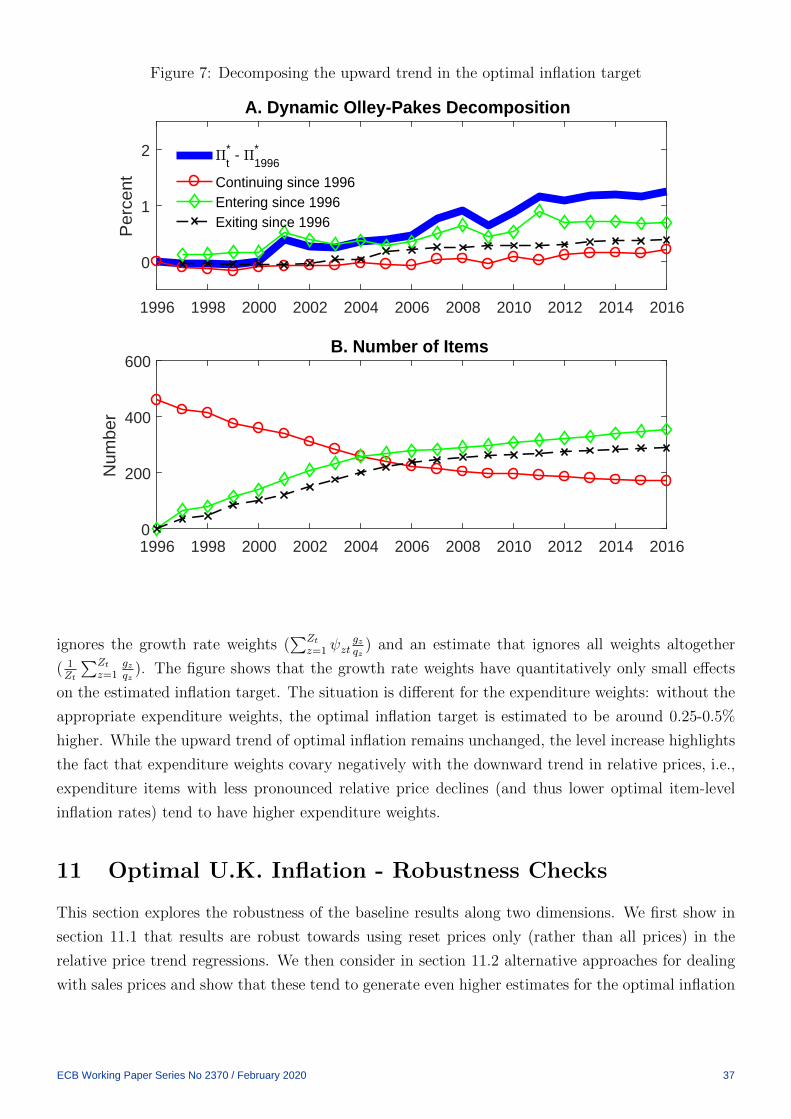
Figure 7: Decomposing the upward trend in the optimal inflation target

1996 1998 2000 2002 2004 2006 2008 2010 2012 2014 2016

0

1

2

Per

cent

A. Dynamic Olley-Pakes Decomposition

*t - *

1996

Continuing since 1996Entering since 1996Exiting since 1996

1996 1998 2000 2002 2004 2006 2008 2010 2012 2014 20160

200

400

600

Num

ber

B. Number of Items

ignores the growth rate weights (∑Zt

z=1 ψztgzqz

) and an estimate that ignores all weights altogether

( 1Zt

∑Ztz=1

gzqz

). The figure shows that the growth rate weights have quantitatively only small effects

on the estimated inflation target. The situation is different for the expenditure weights: without the

appropriate expenditure weights, the optimal inflation target is estimated to be around 0.25-0.5%

higher. While the upward trend of optimal inflation remains unchanged, the level increase highlights

the fact that expenditure weights covary negatively with the downward trend in relative prices, i.e.,

expenditure items with less pronounced relative price declines (and thus lower optimal item-level

inflation rates) tend to have higher expenditure weights.

11 Optimal U.K. Inflation - Robustness Checks

This section explores the robustness of the baseline results along two dimensions. We first show in

section 11.1 that results are robust towards using reset prices only (rather than all prices) in the

relative price trend regressions. We then consider in section 11.2 alternative approaches for dealing

with sales prices and show that these tend to generate even higher estimates for the optimal inflation


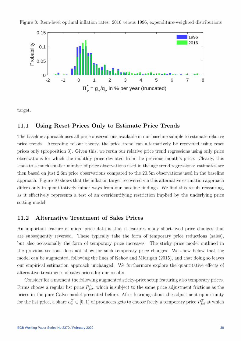
Figure 8: Item-level optimal inflation rates: 2016 versus 1996, expenditure-weighted distributions

-2 -1 0 1 2 3 4 5 6 7 8

z* = g

z/q


0

0.05

0.1

0.15P

roba

bilit

y19962016

-2 -1 0 1 2 3 4 5 6 7 8

z* = g

z/q


0

0.05

0.1

Pro

babi

lity

19962016target.

11.1 Using Reset Prices Only to Estimate Price Trends

The baseline approach uses all price observations available in our baseline sample to estimate relative

price trends. According to our theory, the price trend can alternatively be recovered using reset

prices only (proposition 3). Given this, we rerun our relative price trend regressions using only price

observations for which the monthly price deviated from the previous month’s price. Clearly, this

leads to a much smaller number of price observations used in the age trend regressions: estimates are

then based on just 2.6m price observations compared to the 20.5m observations used in the baseline

approach. Figure 10 shows that the inflation target recovered via this alternative estimation approach

differs only in quantitatively minor ways from our baseline findings. We find this result reassuring,

as it effectively represents a test of an overidentifying restriction implied by the underlying price

setting model.

11.2 Alternative Treatment of Sales Prices

An important feature of micro price data is that it features many short-lived price changes that

are subsequently reversed. These typically take the form of temporary price reductions (sales),

but also occasionally the form of temporary price increases. The sticky price model outlined in

the previous sections does not allow for such temporary price changes. We show below that the

model can be augmented, following the lines of Kehoe and Midrigan (2015), and that doing so leaves

our empirical estimation approach unchanged. We furthermore explore the quantitative effects of

alternative treatments of sales prices for our results.

Consider for a moment the following augmented sticky-price setup featuring also temporary prices.

Firms choose a regular list price PjLzt, which is subject to the same price adjustment frictions as the

prices in the pure Calvo model presented before. After learning about the adjustment opportunity

for the list price, a share αzT ∈ [0, 1) of producers gets to choose freely a temporary price Pj

Tzt at which


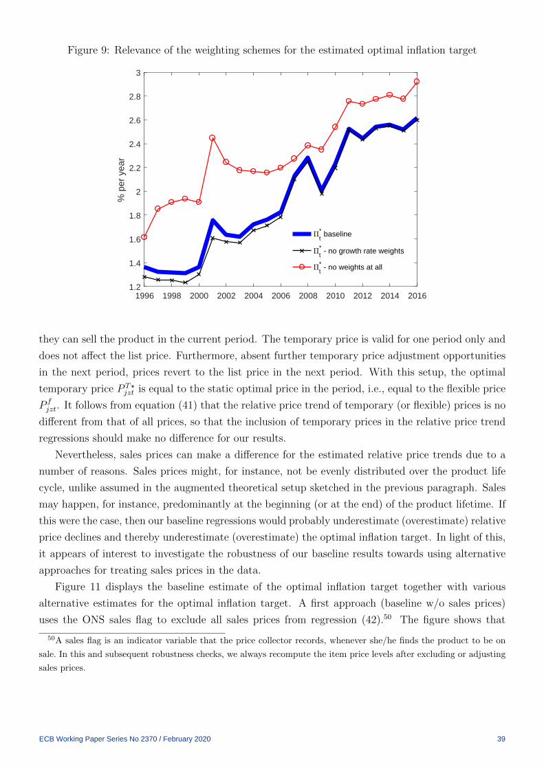
Figure 9: Relevance of the weighting schemes for the estimated optimal inflation target

1996 1998 2000 2002 2004 2006 2008 2010 2012 2014 20161.2

1.4

1.6

1.8

2

2.2

2.4

2.6

2.8

3

% p

er y

ear

t* baseline

t* - no growth rate weights

t* - no weights at all

they can sell the product in the current period. The temporary price is valid for one period only and

does not affect the list price. Furthermore, absent further temporary price adjustment opportunities

in the next period, prices revert to the list price in the next period. With this setup, the optimal

temporary price P T?jzt is equal to the static optimal price in the period, i.e., equal to the flexible price

P fjzt. It follows from equation (41) that the relative price trend of temporary (or flexible) prices is no

different from that of all prices, so that the inclusion of temporary prices in the relative price trend

regressions should make no difference for our results.

Nevertheless, sales prices can make a difference for the estimated relative price trends due to a

number of reasons. Sales prices might, for instance, not be evenly distributed over the product life

cycle, unlike assumed in the augmented theoretical setup sketched in the previous paragraph. Sales

may happen, for instance, predominantly at the beginning (or at the end) of the product lifetime. If

this were the case, then our baseline regressions would probably underestimate (overestimate) relative

price declines and thereby underestimate (overestimate) the optimal inflation target. In light of this,

it appears of interest to investigate the robustness of our baseline results towards using alternative

approaches for treating sales prices in the data.

Figure 11 displays the baseline estimate of the optimal inflation target together with various

alternative estimates for the optimal inflation target. A first approach (baseline w/o sales prices)

uses the ONS sales flag to exclude all sales prices from regression (42).50 The figure shows that

50A sales flag is an indicator variable that the price collector records, whenever she/he finds the product to be on

sale. In this and subsequent robustness checks, we always recompute the item price levels after excluding or adjusting

sales prices.


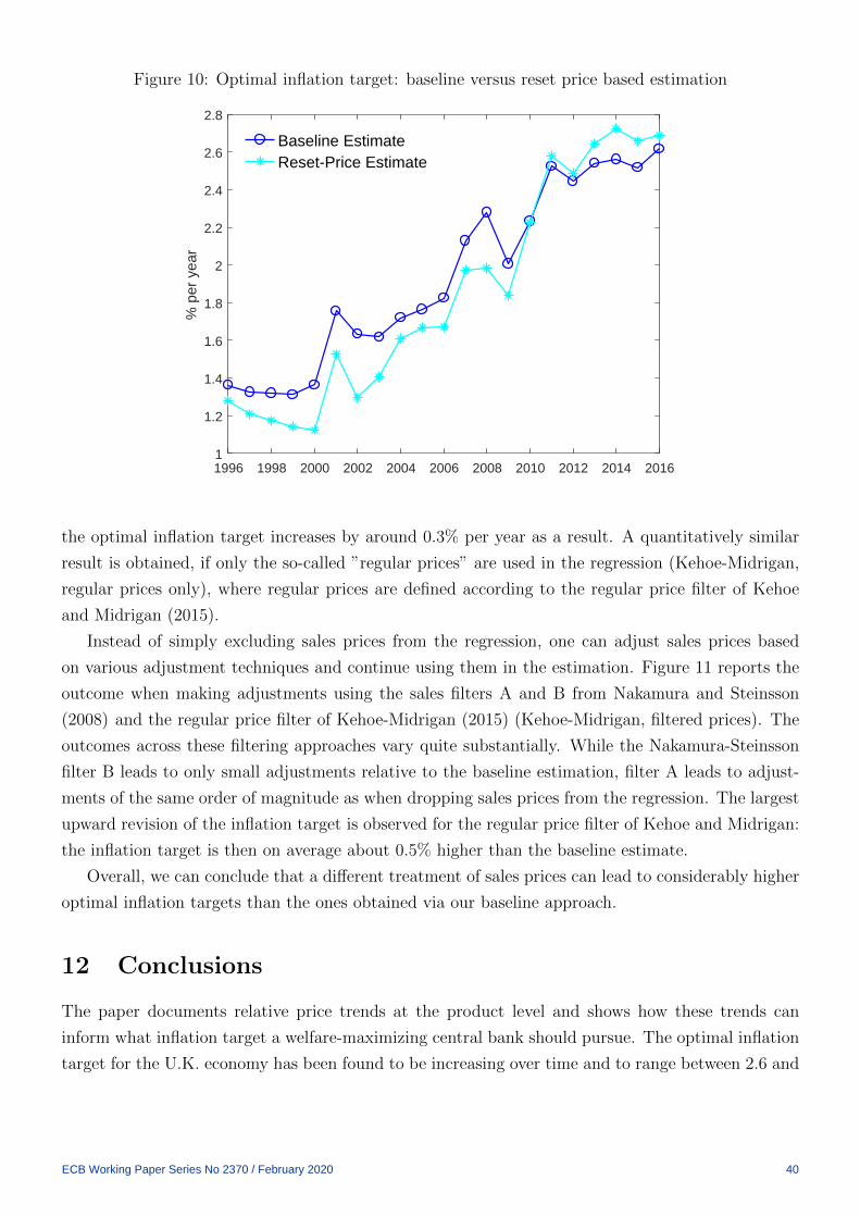
Figure 10: Optimal inflation target: baseline versus reset price based estimation

1996 1998 2000 2002 2004 2006 2008 2010 2012 2014 20161

1.2

1.4

1.6

1.8

2

2.2

2.4

2.6

2.8

% p

er y

ear

Baseline EstimateReset-Price Estimate

the optimal inflation target increases by around 0.3% per year as a result. A quantitatively similar

result is obtained, if only the so-called ”regular prices” are used in the regression (Kehoe-Midrigan,

regular prices only), where regular prices are defined according to the regular price filter of Kehoe

and Midrigan (2015).

Instead of simply excluding sales prices from the regression, one can adjust sales prices based

on various adjustment techniques and continue using them in the estimation. Figure 11 reports the

outcome when making adjustments using the sales filters A and B from Nakamura and Steinsson

(2008) and the regular price filter of Kehoe-Midrigan (2015) (Kehoe-Midrigan, filtered prices). The

outcomes across these filtering approaches vary quite substantially. While the Nakamura-Steinsson

filter B leads to only small adjustments relative to the baseline estimation, filter A leads to adjust-

ments of the same order of magnitude as when dropping sales prices from the regression. The largest

upward revision of the inflation target is observed for the regular price filter of Kehoe and Midrigan:

the inflation target is then on average about 0.5% higher than the baseline estimate.

Overall, we can conclude that a different treatment of sales prices can lead to considerably higher

optimal inflation targets than the ones obtained via our baseline approach.

12 Conclusions

The paper documents relative price trends at the product level and shows how these trends can

inform what inflation target a welfare-maximizing central bank should pursue. The optimal inflation

target for the U.K. economy has been found to be increasing over time and to range between 2.6 and


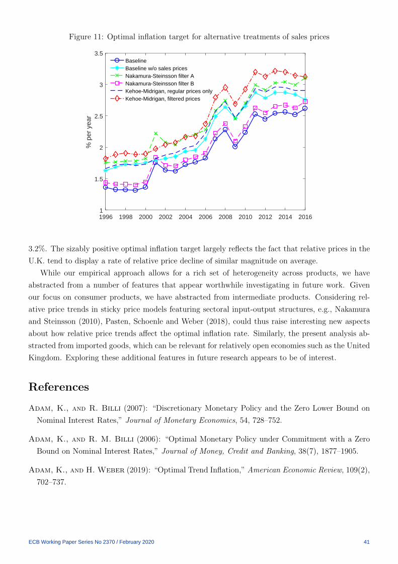
Figure 11: Optimal inflation target for alternative treatments of sales prices

1996 1998 2000 2002 2004 2006 2008 2010 2012 2014 20161

1.5

2

2.5

3

3.5

% p

er y

ear

BaselineBaseline w/o sales pricesNakamura-Steinsson filter ANakamura-Steinsson filter BKehoe-Midrigan, regular prices onlyKehoe-Midrigan, filtered prices

3.2%. The sizably positive optimal inflation target largely reflects the fact that relative prices in the

U.K. tend to display a rate of relative price decline of similar magnitude on average.

While our empirical approach allows for a rich set of heterogeneity across products, we have

abstracted from a number of features that appear worthwhile investigating in future work. Given

our focus on consumer products, we have abstracted from intermediate products. Considering rel-

ative price trends in sticky price models featuring sectoral input-output structures, e.g., Nakamura

and Steinsson (2010), Pasten, Schoenle and Weber (2018), could thus raise interesting new aspects

about how relative price trends affect the optimal inflation rate. Similarly, the present analysis ab-

stracted from imported goods, which can be relevant for relatively open economies such as the United

Kingdom. Exploring these additional features in future research appears to be of interest.

References

Adam, K., and R. Billi (2007): “Discretionary Monetary Policy and the Zero Lower Bound on

Nominal Interest Rates,” Journal of Monetary Economics, 54, 728–752.

Adam, K., and R. M. Billi (2006): “Optimal Monetary Policy under Commitment with a Zero

Bound on Nominal Interest Rates,” Journal of Money, Credit and Banking, 38(7), 1877–1905.

Adam, K., and H. Weber (2019): “Optimal Trend Inflation,” American Economic Review, 109(2),

702–737.


Aghion, P., A. Bergeaud, T. Boppart, P. Klenow, and H. Li (2019): “Missing Growth

from Creative Destruction,” American Economic Review, 109, 2795–2822.

Aghion, P., and P. Howitt (1992): “A Model of Growth through Creative Destruction,” Econo-

metrica, 60(2), 323–351.

Alvarez, F., M. Beraja, M. Gonzalez-Rozada, and P. A. Neumeyer (2019): “From Hyper-

inflation to Stable Prices: Argentina’s Evidence on Menu Cost Models*,” The Quarterly Journal

of Economics, 134(1), 451–505.

Aoki, K. (2001): “Optimal monetary policy responses to relative-price changes,” Journal of Mone-

tary Economics, 48(1), 55 – 80.

Argente, D., M. Lee, and S. Moreira (2018): “How Do Firms Grow? The Life Cycle of

Products Matters,” University of Chicago mimeo.

Argente, D., and C. Yeh (2018): “Product Life Cycle, Learning, and Nominal Shocks,” Univer-

sity of Chicago mimeo.

Benigno, P. (2004): “Optimal monetary policy in a currency area,” Journal of International Eco-

nomics, 63(2), 293 – 320.

Benigno, P., and L. A. Ricci (2011): “The Inflation-Output Trade-Off with Downward Wage

Rigidities,” American Economic Review, 101, 1436–1466.

Bergin, P. R., and G. Corsetti (2008): “The extensive margin and monetary policy,” Journal

of Monetary Economics, 55(7), 1222–1237.

Bilbiie, F. O., I. Fujiwara, and F. Ghironi (2014): “Optimal monetary policy with endogenous

entry and product variety,” Journal of Monetary Economics, 64, 1–20.

Bilbiie, F. O., F. Ghironi, and M. J. Melitz (2008): “Monetary Policy and Business Cycles

with Endogenous Entry and Product Variety,” in NBER Macroeconomics Annual 2007, Volume

22, NBER Chapters, pp. 299–353. National Bureau of Economic Research, Inc.

Bils, M. (2009): “Do Higher Prices for New Goods Reflect Quality Growth or Inflation?,” Quarterly

Journal of Economics, 124, 637–675.

Blanco, A. (2019): “Optimal Inflation Target in an Economy with Menu Costs and Zero Lower

Bound,” University of Michigan mimeo.

Broda, C., and D. E. Weinstein (2010): “Product Creation and Destruction:Evidence and Price

Implications,” American Economic Review, 100, 691–723.

Bunn, P., and C. Ellis (2012): “Examining The Behaviour Of Individual UK Consumer Prices,”

The Economic Journal, 122(558), F35–F55.


Burstein, A., and C. Hellwig (2008): “Welfare Costs of Inflation in a Menu Cost Model,”

American Economic Review, Papers and Proceedings,, 98 (2), 438–443.

Carlsson, M., and A. Westermark (2016): “Labor market frictions and optimal steady-state

inflation,” Journal of Monetary Economics, 78, 67 – 79.

Coibion, O., Y. Gorodnichenko, and J. Wieland (2012): “The Optimal Inflation Rate in

New Keynesian Models: Should Central Banks Raise Their Inflation Targets in Light of the Zero

Lower Bound?,” Review of Economic Studies, 79(4), 1371–1406.

Dixit, A. (1991): “Analytical Approximations in Models of Hysteresis,” The Review of Economic

Studies, 58(1), 141–151.

Ernesto Pasten, R. S., and M. Weber (2018): “The Propagation of Monetary Policy Shocks

in a Heterogeneous Production Economy,” Brandeis University Mimeo.

Golosov, M., and R. E. Lucas (2007): “Menu Costs and Phillips Curves,” Journal of Political

Economy, 115, 171–199.

Hahn, V., and M. Marencak (2018): “Price Points and Price Dynamics,” Working Paper Series

of the Department of Economics, University of Konstanz 2018-01, Department of Economics,

University of Konstanz.

Kehoe, P. J., and V. Midrigan (2015): “Prices Are Sticky After All,” Journal of Monetary

Economics, 75, 35–53.

Khan, A., R. G. King, and A. L. Wolman (2003): “Optimal Monetary Policy,” Review of

Economic Studies, 70, 825–860.

Kim, J., and F. J. Ruge-Murcia (2009): “How much inflation is necessary to grease the wheels?,”

Journal of Monetary Economics, 56(3), 365 – 377.

Klepper, S. (1996): “Entry, Exit, Growth, and Innovation over the Product Life Cycle,” American

Economic Review, 86(3), 562–583.

Kryvtsov, O., and N. Vincent (2017): “The Cyclicality of Sales and Aggregate Price Flexibility,”

Working paper available at https://sites.google.com/site/okryvtsov/.

Melitz, M. J., and S. Polanec (2015): “Dynamic Olley-Pakes productivity decomposition with

entry and exit,” The RAND Journal of Economics, 46(2), 362–375.

Melser, D., and I. A. Syed (2016): “Life Cycle Price Trends and Product Replacement: Impli-

cations for the Measurement of Inflation,” Review of Income and Wealth, 62, 509–533.

Nakamura, E., and J. Steinsson (2008): “Five Facs about Prices: A Reevaluation of Menu Cost

Models,” Quarterly Journal of Economics, 123, 1415–1464.


(2010): “Monetary Non-neutrality in a Multisector Menu Cost Model,” The Quarterly

Journal of Economics, 125(3), 961–1013.

Office for National Statistics (2014): Consumer Price Indices - Technical Manual.

Schmitt-Grohe, S., and M. Uribe (2010): “The Optimal Rate of Inflation,” in Handbook of

Monetary Economics, ed. by B. M. Friedman, and M. Woodford, vol. 3 of Handbook of Monetary

Economics, chap. 13, pp. 653–722. Elsevier.

(2012): “On Quality Bias and Inflation Targets,” Journal of Monetary Economics, 59(4),

393 – 400.

Shleifer, A. (1986): “Implementation Cycles,” Journal of Political Economy, 94(6), 1163–1190.

Wolman, A. L. (2011): “The Optimal Rate of Inflation with Trending Relative Prices,” Journal

of Money, Credit and Banking, Vol. 43, 355–384.


A Key Model Derivations

A.1 First-Order Conditions of the Household Problem

The representative household maximizes expected discounted utility in equation (2) subject to the

budget constraint (3). The first-order conditions to this maximization problem comprise

Wt

Pt= −Ct

∂V (Lt)/∂LtV (Lt)

(48)

Ωt,t+1 = β

(Ct+1

Ct

)−σ (V (Lt+1)

V (Lt)

)1−σ

(49)

1 = Et

[Ωt,t+1

(1 + itPt+1/Pt

)](50)

1 = Et [Ωt,t+1(rt+1 + 1− d)] , (51)

a no-Ponzi scheme condition, the transversality condition and the household’s budget constraint.

A.2 Derivation of Firms’ Marginal Cost Expression (21)

Let

Ijzt ≡ Yjzt/(AztQjztGjzt)

denote the units of factor inputs (K1− 1

φ

jzt L1φ

jzt) required to produce Yjzt units of (quality-adjusted)

output. We now show that cost minimization yields the expression for nominal marginal costs of Ijzt

provided in equation (21). Firm j chooses the factor input mix to minimize production costs subject

to the constraint imposed by the production function (6),

minKjzt,Ljzt

Kjztrt + LjztWt/Pt s.t. Yjzt = AztQjztGjztK1− 1

φ

jzt L1φ

jzt .

Denoting the Lagrange multiplier by λt, this cost minimization problem yields first-order conditions

0 = rt +

(1− 1

φ

)λtAztQjztGjzt

(LjztKjzt

) 1φ

0 = Wt/Pt +1

φλtAztQjztGjzt

(LjztKjzt

) 1φ−1

.

These conditions imply that the optimal capital labor ratio is the same for all firms j ∈ [0, 1] and all

items z = 1, . . . Zt, i.e.,Kjzt

Ljzt=

Wt

Ptrt(φ− 1). (52)

Substituting the optimal factor input mix into the production function (6) and solving for the factor

inputs yields the factor demand functions

Ljzt =

(Wt

Ptrt(φ− 1)

) 1φ−1

Ijzt (53)

Kjzt =

(Wt

Ptrt(φ− 1)

) 1φ

Ijzt, (54)


where Ijzt is defined in the text. Firm j demands these amounts of labor and capital, respectively,

to combine them to Yjzt units of (quality-adjusted) output. Thus, the firm’s cost function is

MCtIjzt = Wt

(Wt

Ptrt(φ− 1)

) 1φ−1

Ijzt + Ptrt

(Wt

Ptrt(φ− 1)

) 1φ

Ijzt, (55)

where MCt denotes nominal marginal (or average) costs. The previous equation can be rearranged

to obtain equation (21).

A.3 Derivation of the Optimal Price Setting Equation (25)

The first order condition to the firm’s price setting problem (22) yields

0 = Et

∞∑i=0

(αz(1− δz))iΩt,t+i

Pt+iYjzt+i

[P ?jzt −

θ

(1 + τ)(θ − 1)

(MCt+i

Azt+iQzt+iQjzt+i

)],

where we use the short-hand notation Qjzt = QjztGjzt/Qzt. Solving this equation for P ?jzt yields

P ?jzt

PtQjzt =

(1

1 + τ

θ

θ − 1

)(56)

Et∑∞

i=0(αz(1− δz))iΩt,t+i

(Pzt+iPzt

)θ−1 (Pt+iPt

Yt+iYt

)(MCt+i

Pt+iAzt+iQzt+i

)(QjztQjzt+i

)Et∑∞

i=0(αz(1− δz))iΩt,t+i

(Pzt+iPzt

)θ−1 (Yt+iYt

) .

We can express the ratio Qjzt/Qjzt+i in the previous equation as

QjztQjzt+i

=GjztQzt+i

Gjzt+iQzt

,

because quality remains constant over the lifetime of product j, so that Qjzt = Qjzt+i. Using equation

(7) to substitute for productivity Gjzt and the fact that the idiosyncratic component εGjzt remains

constant of the product lifetime further yields

QjztQjzt+i

=Gjzt

Gjzt+i

Qzt+i

Qzt

.

Given the evolution of Gjzt implied by equation (9), this equation can be rearranged to obtain

QjztQjzt+i

=

∏ik=1 qzt+k∏ik=1 gzt+k

,

which is independent of the product index j and reduces to Qjzt/Qjzt+i = 1 for i = 0. Using the

previous equation, we can express the numerator on the r.h.s. of equation (56), denoted by Nzt,

recursively as

Nzt =MCt

PtAztQzt

+ αz(1− δz)Et

[Ωt,t+1

(Pzt+1

Pzt

)θ−1(Pt+1

Pt

)(Yt+1

Yt

)(qzt+1

gzt+1

)Nzt+1

]. (57)

We can also express the denominator on the r.h.s. of equation (56), denoted by Dzt, recursively as

Dzt = 1 + αz(1− δz)Et

[Ωt,t+1

(Pzt+1

Pzt

)θ−1(Yt+1

Yt

)Dzt+1

], (58)

which then leads to equation (25) for the optimal price.


A.4 Item Price Level and Its Recursive Evolution Equation

We derive a recursive representation of the item price level Pzt in two steps. First, we decompose

the price level into the prices of newly entering products, the prices of existing products that are

optimally reset in period t, and all remaining prices. Second, we show that optimal reset prices

for existing products with age s ≥ 1 can be expressed as a function of the optimal prices of newly

entering products. This relationship allows us to derive the recursive price-level representation. The

derivation in the present section follows similar steps as in Adam and Weber (2019) but generalizes

it by allowing for idiosyncratic components in productivity and product quality.

From equation (15), we have

P 1−θzt =

∫ 1

0

P 1−θjzt dj,

where Pjzt = Pjzt/Qjzt denotes the quality-adjusted price of product j in item z. We decompose

this price level into (i) all prices that are adjusted in period t, including prices for newly entering

products; (ii) the sticky prices of continuing products. The share of the latter is equal to αz(1− δz)and their average price is equal to the lagged item price level. Thus, applying this decomposition to

the previous equation yields

P 1−θzt =

∞∑s=0

∫J?t−s,t

(P ?jzt)

1−θdj + αz(1− δz)(Pzt−1)1−θ, (59)

where J?t−s,t denotes the set of products with age s in period t that can adjust prices in t. The share

of products that can adjust prices in t is equal to δz + (1− δz)(1−αz), where δz is the share of newly

entering products (all with optimal prices) and (1− δz)(1− αz) is the share of continuing products

that can adjust prices. We can define the average optimal price of products newly entering in t as

P ?z,t,t ≡

(1

δz

∫J?t,t

(P ?jzt)

1−θdj

) 11−θ

, (60)

and the average optimal price of products that entered in t− s (for s ≥ 1) and reset prices in t as

P ?z,t−s,t ≡

(1

(1− αz)δz(1− δz)s

∫J?t−s,t

(P ?jzt)

1−θdj

) 11−θ

. (61)

Substituting the previous two definitions into equation (59) yields

P 1−θzt = δz(P

?z,t,t)

1−θ + (1− αz)δz∞∑s=1

(1− δz)s(P ?z,t−s,t)

1−θ + αz(1− δz)(Pzt−1)1−θ, (62)

where (1− αz)δz∑∞

s=1(1− δz)s + αz(1− δz) = 1− δz is equal to the share of continuing products.

In the second step, we use the optimal price setting equation (25) to express the item price level in

the previous equation recursively. Consider the pricing equation for product j with age sjzt = s ≥ 1

and rewrite (25) by substituting Gjzt using equation (7) and substituting Qjzt using equation (11).

This yieldsP ?jzt

Pt

(Qzt−sGjzt

Qzt

)[εQjz,t−sε

Gjz,t−s] =

(θ

θ − 1

1

1 + τ

)Nzt

Dzt

, (63)


where the term in brackets captures the idiosyncratic component of the optimal price, which is

constant over the product’s lifetime. Since the previous equation refers to products with the same

age, we can use equation (9) to rewrite Gjzt and equation (12) to rewrite Qzt−s/Qzt. This yields

P ?jzt

Pt

(∏s−1k=0 gzt−k∏s−1k=0 qzt−k

)[εQjz,t−sε

Gjz,t−s] =

(θ

θ − 1

1

1 + τ

)Nzt

Dzt

.

Rearranging the previous equation to obtain the average of the optimal prices of products with the

same age s, as defined in equation (61), yields

P ?z,t−s,t =


)−1(θ

θ − 1

1

1 + τ

)NztPtDzt

, (64)

where we used E[(εGjzt)θ−1] = 1 and E[(εQjzt)

θ−1] = 1 and the fact that εGjzt and εQjzt are independent.

Analogous steps for the case of products that newly entering in period t deliver the following

expression for the optimal average price P ?z,t,t of these products, as defined in equation (60):

P ?z,t,t =

(θ

θ − 1

1

1 + τ

)NztPtDzt

. (65)

Equations (64) and (65) jointly deliver

P ?z,t−s,t = P ?

z,t,t


)−1

, (66)

for s ≥ 1. This equation shows how the optimal average price of older products is related to the

optimal average price of newly entering products. Using the previous equation to substitute for

P ?z,t−s,t in equation (62) and rearranging the result yields

P 1−θzt = (P ?

z,t,t)1−θ

αzδz + (1− αz)

δz +∞∑s=1

δz(1− δz)s(∏s−1

k=0 gzt−k∏s−1k=0 qzt−k

)θ−1

+ αz(1− δz)(Pzt−1)1−θ. (67)

Now define

(∆ezt)

1−θ ≡ δz +∞∑s=1



)θ−1

, (68)

and substitute this definition into equation (67). This delivers the recursive representation of the

item price level:

P 1−θzt =

αzδz + (1− αz)(∆e

zt)1−θ (P ?

z,t,t)1−θ + αz(1− δz)(Pzt−1)1−θ, (69)

where P ?z,t,t is defined in equation (60). Finally, we rewrite the definition of ∆e

zt according to

(∆ezt)

1−θ = δz + (1− δz)(gztqzt

)θ−1δz +

∞∑s=1


k=0 gzt−1−k∏s−1k=0 qzt−1−k

)θ−1

= δz + (1− δz)(∆zet−1qzt/gzt

)1−θ,

(70)


which shows that (∆ezt)

1−θ is a stationary variable that evolves recursively. We define the item-level

(gross) inflation rate as

Πzt ≡ Pzt/Pzt−1

and the relative price p?zt as

p?zt ≡ P ?z,t,t/Pzt. (71)

Using these definitions, we rearrange equation (69) to obtain

1 =αzδz + (1− αz)(∆e

zt)1−θ (p?zt)

1−θ + αz(1− δz)(Πzt)θ−1. (72)

The previous equation shows that in a balanced growth path with a constant item-level inflation Πz,

the relative price p?z is also constant.

A.5 Item-Level and Economy-Wide Aggregate Production Functions

We aggregate the model in two steps. In a first step, we aggregate firm-specific production functions

to item-level production functions. In a second step, we aggregate the item-level production functions

to a economy-wide production function.

To obtain the item-level production function, we substitute (quality-adjusted) output of product

j in item z in the production function (6) using the demand function (18). This yields

YztAztQjztGjzt

(PjztPzt

)−θ=

(Kjzt

Ljzt

)1− 1φ

Ljzt .

Integrating the previous equation over all firms j ∈ [0, 1] in item z, using the definition

Lzt ≡∫Ljzt dj,

and equation (52), which shows that capital-to-labor ratio is identical for all products, we obtain the

item-level production function for quality-adjusted output in item z

Yzt =AztQzt

∆zt

(K

1− 1φ

zt L1φ

zt

), (73)

where

Kzt ≡∫Kjzt dj

and where we have defined the productivity parameter 1/∆zt as

∆zt ≡∫ 1

0

(Qzt

QjztGjzt

)(PjztPzt

)−θdj , (74)

which captures the (detrended) distribution of productivities and qualities across products in item

z. The recursive evolution equation for ∆zt is derived in appendix A.6.

To obtain the economy-wide aggregate production function, we rewrite equation (73) to obtain

Yzt∆zt

AztQzt

=

(Kt

Lt

)1− 1φ

Lzt.


where we used the fact that the capital-to-labor ratio is the same across items, see equation (52).

Summing the previous equation over all items z = 1, ..Z, and using labor market clearing across

items, Lt =∑

z Lzt, and the demand function (19) to substitute for item-level output Yzt, we obtain

Yt

Zt∑z=1

ψzt

(PztPt

)−1(∆zt

AztQzt

)= K

1− 1φ

t L1φ

t .

The aggregate economy-wide production function for quality-adjusted output is thus given by

Yt =(Γet )

1/φ

∆t

(K

1− 1φ

t L1φ

t

), (75)

where the aggregate economy-wide productivity parameter 1/∆t is defined according to

∆t ≡ (Γet )1/φ

Zt∑z=1

ψzt

(PztPt

)−1(∆zt

AztQzt

), (76)

and where Γet denotes the trend-growth factor defined in Appendix B.4 and ensures that ∆t a sta-

tionary variable.

A.6 Derivation of the Recursive Evolution Equation for ∆zt

To derive a recursive representation for the productivity shifter ∆zt, defined in equation (74), we

decompose it in a way that resembles the decomposition of the item price level in Appendix A.4.

This yields

∆zt

P θzt

=∞∑s=0

∫J?t−s,t

(Qzt

QjztGjzt

)(P ?

jzt)−θdj +

qztgzt

∫Jt

(Qzt−1

Qjzt−1Gjzt−1

)(Pjzt−1)−θdj, (77)

where, as before, J?t−s,t denotes the set of products with age s ≥ 0 at time t that can adjust prices

in t. Let Jt denote the set of all products that can not adjust prices in t. To derive equation (77),

we have used the fact that all products in Jt have age s ≥ 1. We have also used the fact that the

productivity component Gjzt for the products in Jt−1,t continues to evolve over time, which yields

Gjzt = Gjzt · εGjzt−1

=

(Gjzt

Gjzt−1

)(Gjzt−1 · εGjzt−1

)= gztGjzt−1, (78)

where the last line follows from equations (7) and (9) for the case with s ≥ 1.

Since products in Jt are a representative subset of all products in the economy at date t− 1 and

since Jt has mass αz(1− δz), we can rewrite equation (77) by shifting equation (74) one period into

the past, which yields

∆zt

P θzt

=∞∑s=0

∫J?t−s,t

(Qzt

QjztGjzt

)(P ?

jzt)−θdj + αz(1− δz)

qztgzt

∆zt−1

P θzt−1

. (79)


We now rearrange the infinite sum in the previous equation. The steps involved in this resemble the

steps used in in the derivation of the item price level in Appendix A.4, but with slight modifications.

We first show how the integrals appearing in the infinite sum on the r.h.s. of equation (79) are

related to the average optimal price of newly entering products P ?z,t,t. For s ≥ 1, we obtain∫

J?t−s,t

(Qzt

QjztGjzt

)(P ?

jzt)−θdj =

(∏s−1k=0 qzt−k∏s−1k=0 gzt−k

)∫J?t−s,t

[Qzt−s

Qjzt−sGjzt−s

](P ?

jzt)−θdj, (80)

using Qzt = (∏s−1

k=0 qzt−k)Qzt−s and the fact that products in J?t−s,t have age greater or equal to s.

We can rearrange the r.h.s. of equation (80) further using

Gjzt =

(s−1∏k=0

gzt−k

)Gjzt−s,

which follows from (78). The brackets in equation (80) contain only idiosyncratic components and

thus simplify asQzt−s

Qjzt−sGjzt−s= [εQjz,t−sε

Gjz,t−s]

−1.

Substituting the previous two equations into equation (80) and integrating the result over the prod-

ucts in J?t−s,t yields

∫J?t−s,t

(Qzt

QjztGjzt

)(P ?

jzt)−θdj =


)−1 ∫J?t−s,t

[εQjz,t−sεGjz,t−s]

−1(P ?jzt)−θdj. (81)

To link the previous equation to the average optimal price of newly entering products P ?z,t,t, we

rearrange equation (64) to obtain


−1(P ?jzt)−θ = [εQjz,t−sε

Gjz,t−s]

θ−1


)−1(θ

θ − 1

1

1 + τ

)NztPtDzt

−θ .Integrating the previous equation over the set of products in J?t−s,t and normalizing the result yields

∫J?t−s,t


−1

(1− αz)δz(1− δz)s(P ?

jzt)−θ dj =


)−1(θ

θ − 1

1

1 + τ

)NztPtDzt

−θ ,where we used E[(εGjzt)

θ−1] = 1 and E[(εQjzt)θ−1] = 1 and the fact that εGjzt and εQjzt are independent.

We can now use equation (65) to substitute P ?z,t,t into the previous equation, which yields

∫J?t−s,t


−1

(1− αz)δz(1− δz)s(P ?

jzt)−θ dj =


)θ (P ?z,t,t

)−θ.

Furthermore, substituting the previous equation for the r.h.s. of equation (81) yields∫J?t−s,t

(Qzt

QjztGjzt

)(P ?

jzt)−θdj = (1− αz)δz(1− δz)s


)θ−1 (P ?z,t,t

)−θ,


which shows how the integral terms on the r.h.s. of equation (79) are related to the average optimal

price of newly entering products P ?z,t,t for s ≥ 1. For the case with s = 0, analogous steps yield∫

J?t,t

[εQjztεGjzt]−1(P ?

jzt)−θ dj = δz(P

?z,t,t)

−θ.

Using the preceding two equations to substitute for the integrals in the infinite sum on the r.h.s. of

equation (79), we obtain

∆zt

P θzt

= (P ?z,t,t)

−θ

δz + (1− αz)∞∑s=1



)θ−1+ αz(1− δz)

qztgzt

∆zt−1

P θzt−1

,

where the term in curly brackets is the same as the term in curly brackets in equation (67). Accord-

ingly, rearranging the previous equation yields the recursive representation

∆zt = (p?zt)−θ αzδz + (1− αz)(∆e

zt)1−θ+ αz(1− δz)(Πzt)

θ (gzt/qzt)−1 ∆zt−1,

where Πzt = Pzt/Pzt−1. The stationary variable ∆ezt evolves as described in equation (70) and p?zt is

defined in equation (71). The previous equation shows that ∆zt is constant in the balanced growth

path, because p?zt is constant in this path due to equation (72).

B Efficient Allocation and Efficient Growth Trends

As a reference point and to better understand the distortions emerging in the decentralized economy,

this section derives the first-best allocation. This involves deriving the allocation of factor inputs

across products with different levels of product quality and productivity at the level of each expen-

diture item z, in addition to the allocation of factor inputs across items z with different average

quality and productivity. It also requires determining the optimal intertemporal paths of aggregate

variables. This appendix also derives the growth trend of variables in the efficient allocation. Using

the efficient trends we drive expressions for the efficient allocation in terms of detrended variables.

Throughout the appendix, variables carrying the superscript ’e’ denote efficient quantities.

B.1 Efficient Allocation at the Item-Level

Consider a setting where it is efficient to allocate Lezt units of labor and Kezt units of capital to the

production of products in item z. The optimal allocation of capital and labor across products j in

item z maximizes then (quality-adjusted) item-level output/consumption in equation (5), subject to

the production function (6) and the feasibility constraints Lezt =∫zLejzt dj and Ke

zt =∫zKejzt dj. This

allocation problem yields the efficient item-level output

Y ezt =

AztQzt

∆ezt

(Kezt)

1− 1φ (Lezt)

1φ , (82)


where the efficient productivity parameters 1/∆ezt is defined as

1/∆ezt ≡

(∫ 1

0

(GjztQjzt/Qzt)θ−1 dj

) 1θ−1

. (83)

To derive a recursive representation for 1/∆ezt, we rearrange the previous equation to obtain

(∆ezt)

1−θ = δz

∞∑s=0

(1− δz)s1

δz(1− δz)s

∫Jt−s,t

(GjztQjzt/Qzt)θ−1 dj, (84)

where Jt−s,t denotes the set of products with age s ≥ 0 in period t. The integrals appearing on the

r.h.s. of the infinite sum in the previous equation can bet expressed as

1

δz(1− δz)s

∫Jt−s,t

(GjztQjzt/Qzt)θ−1 dj =


)θ−1

,

since E[(εQjzt)θ−1] = 1 and E[(εGjzt)

θ−1] = 1 and εQjzt and εGjzt are independent. Plugging the previous

equation into equation (84) yields equation (68) which as is shown in appendix A.4, has the recursive

representation described in equation (70).

B.2 Efficient Allocation Across Items

The optimal allocation of capital and labor between items maximizes (quality-adjusted) aggregate

output/consumption in equation (4), subject to the efficient item-level production function (82) and

the feasibility conditions Let =∑

z Lezt and Ke

t =∑

zKezt, for given levels of Let and Ke

t . Solving this

allocation problem delivers the aggregate economy-wide efficient production function

Y et =

(Γet )1/φ

∆et

(Ket )

1− 1φ (Let )

1φ , (85)

where the efficient productivity level 1/∆et is defined as

1

∆et

≡ (Γet )− 1φ

(Zt∏z=1

ψψztzt

(AztQzt

∆ezt

)ψzt), (86)

and Γet denotes the aggregate growth rate defined in Appendix B.4 and ensures that ∆et a stationary

variable.

B.3 Efficient Intertemporal Allocation

The intertemporal allocation maximizes expected discounted utility of the representative household,

equation (2), subject to the intertemporal feasibility condition

Cet +Ke

t+1 = (1− d)Ket + Y e

t (87)


and the aggregate economy-wide production function (85). The first order conditions to this problem

comprise the feasibility condition (87) and

Y eLt = −U

eLt

U eCt

, (88)

1 = βEt

[U eCt+1

U eCt

(Y eKt+1 + 1− d

)], (89)

where UCt denotes the marginal utility of consumption in t, ULt the marginal disutility from labor,

Y eKt the marginal product of capital and Y e

Lt the marginal product of labor.

B.4 Efficient Item-Level and Aggregate Growth Trends

This section determined the efficient growth for the balanced growth path equilibrium in which

aggregate hours worked Let and item-level hours worked Lezt are stationary for all z. The variables

Cet , K

et and Y e

t all display the same growth trend, which we denote by Γet . Since the captial-to-labor

ratio is constant across products, it then follows the item-level capital stocks Kzt have the same

growth trend Γet for all z.

We can then derive the item-level output growth trend by rewriting equation (82) as

Y ezt =

AztQzt

∆ezt

(Γet )1− 1

φ

(Kezt

Γet

)1− 1φ

(Lezt)1φ ,

which shows that Y ezt grows at the same rate as AztQzt

∆ezt

(Γet )1− 1

φ because all other variables are stationary.

We can thus define the item-level growth trend as

Γezt ≡AztQzt

∆ezt

(Γet )1− 1

φ . (90)

To derive the aggregate growth trend Γet , we substitute equilibrium output for equilibrium consump-

tion in equation (4) and detrend all output variables in the resulting equation by their respective

growth trends, which yields

Y et

Γet=

[∏Ztz=1(Γezt)

ψzt

Γet

]Zt∏z=1

(Y ezt

Γezt

)ψzt.

Since Y ezt/Γ

ezt is stationary, the the aggregate growth trend is given by

Γet ≡Zt∏z=1

(Γezt)ψzt . (91)

Using definition (90) to substitute for Γezt in the previous equation and solving for Γet yields

Γet =Zt∏z=1

(AztQzt

∆ezt

)φψzt, (92)


which determines the aggregate growth trend in terms of model primitives. Substituting the previous

equation for Γet into equation (90) shows that the item-level growth trend relative to the aggregate

growth trend is independent of the parameter φ and given by

ΓeztΓet

=

(AztQzt

∆ezt

)∏Zt

z=1

(AztQzt

∆ezt

)ψzt . (93)

We also define the aggregate growth rate as

γet ≡ Γet/Γet−1. (94)

Using equation (92) to substitute for Γet and Γet−1 we obtain:

γe =Z∏z=1

(azqz)ψzφ (95)

in the steady state. Furthermore, we define the item-level growth rate as

γezt ≡ Γezt/Γezt−1, (96)

and using equation (93), we obtain that in steady state,

γezγe

=azqz∏Z

z=1 (azqz)ψz.

B.5 Efficient Production in Terms of Detrended Variables

We now express the item-level and aggregate production functions in the planned economy in terms

of detrended output and capital variables. Letting lower case letters denote stationary variables,

we can defineyet ≡ Y et /Γ

et , k

et ≡ Ke

t /Γet , k

ezt ≡ Ke

zt/Γet and yezt ≡ Y e

zt/Γezt. To obtain the production

function in item z in terms of detrended variables, we divide equation (82) by equation (90) and use

the definitions of item-level detrended variables. This yields

yezt = (kezt)1− 1

φ (Lezt)1φ . (97)

To obtain the aggregate production function in terms of detrended variables, we divide equation (85)

by Γet and use the definitions of aggregate detrended variables, which yields

yet =1

∆et

(ket )1− 1

φ (Let )1φ . (98)

Here, 1/∆et is defined in equation (86), and this definition simplifies to

1

∆et

=Zt∏z=1

ψψztzt , (99)

after substituting the equation (92) for Γte into the definition.


C The Decentralized Economy and its Distortions

We now express the prices and allocations in the decentralized economy in terms of detrended vari-

ables, using the efficient growth trends derived in the previous appendix to detrend quantities. We

then relate the allocation in the decentralized economy to the first-best allocation derived in the pre-

vious section using two key distortions (or wedges), namely a mark-up distortion and a relative-price

distortion.

Appendices C.1 and C.2 start by deriving the growth trends of relative prices and express optimal

reset prices in terms of detrended variables. Appendix C.3 introduces the mark-up distortion and

uses it to rewrite various first-order conditions of households and firms. Appendix C.4 derives the

item-level and aggregate production functions for the decentralized economy and relates them to the

efficient allocation by introducing a relative-price distortion term. Appendix C.5 summarizes the

equations characterizing the decentralized economy in detrended variables.

C.1 Relative Price Trends and Relative Inflation Rates

To detrend the relative price of item z, Pzt/Pt, we multiply the demand function (19) by the (inverse

of the) relative growth factor Γezt/Γet , which yields

yzt/yt = ψztp−1zt , (100)

where we have defined

pzt ≡ (Pzt/Pt) (Γezt/Γet ) , (101)

which is constant in steady state. The demand function (19) also implies

Πzt

Πt

=

(ψztψzt−1

)(γeztyzt/yzt−1

γetyt/yt−1

)−1

,

which shows that items with stronger price increases face stronger output declines, which is a result

of Cobb-Douglas aggregation across expenditure items.

C.2 Optimal Price in Terms of Detrended Variables

To express the optimal reset price in equation (25) in terms of detrended variables, we multiply the

equation by the relative sectoral growth trend, Γezt/Γet (see Appendix B) and divide by item price

level Pzt. This yields

P ?jzt

Pzt

(QjztGjzt

Qzt

)pzt =

(1

1 + τ

θ

θ − 1

)Nzt

Dzt

(ΓeztΓet

), (102)

where pzt is defined in equation (101). Since Dzt is stationary, see equation (58), we can define

dzt ≡ Dzt. (103)


The variable Nzt in equation (102) grows over time, but the variable

nzt ≡ Nzt

(ΓeztΓet

)(104)

is again stationary, as we show below. Using these definitions, we can thus write equation (102) in

terms of stationary variables according to

P ?jzt

Pzt

(QjztGjzt

Qzt

)pzt =

(1

1 + τ

θ

θ − 1

)nztdzt

. (105)

It remains to prove the stationarity of nzt. Using the definition of nzt and equation (57) delivers

nzt =

(MCt

PtAztQzt

)(ΓeztΓet

)+ αz(1− δz)Et

[Ωt,t+1

(Pzt+1

Pzt

)θ−1(Pt+1

Pt

)(Yt+1

Yt

)(qzt+1

gzt+1

)(ΓeztΓet

)(Γezt+1

Γet+1

)−1

nzt+1

]or equivalently

nzt =

(MCt

PtAztQzt

)(ΓeztΓet

)+ αz(1− δz)Et

[Ωt,t+1Πθ−1

zt+1Πt+1 (yt+1/yt) γet+1

(qzt+1

gzt+1

)(γet+1

γezt+1

)nzt+1

]. (106)

We can rewrite equation (90) to obtain

ΓeztΓet

= (Γet )− 1φ

(AztQzt

∆ezt

),

and use this equation to rearrange the term involving marginal costs in equation (106) according to(MCt

PtAztQzt

)(ΓeztΓet

)=

(MCt

PtAztQzt

)(Γet )

− 1φ

(AztQzt

∆ezt

)=

(MCt

Pt(Γet )1/φ

)(1

∆ezt

).

We then define real detrended marginal costs as

mct ≡MCt

Pt(Γet )1/φ, (107)

where MCt is defined in equation (21). Substituting the previous equation into equation (106) yields

nzt =mct∆ezt

+ αz(1− δz)Et[Ωt,t+1Πθ−1


(qzt+1

gzt+1

)(γet+1

γezt+1

)nzt+1

],

which contains only stationary variables. From equation (58) and the definition of dzt we likewise

obtain

dzt = 1 + αz(1− δz)Et[Ωt,t+1Πθ−1

zt+1 (yt+1/yt) γet+1dzt+1

].

To obtain a detrended expression for the average optimal price of new products, we integrate

equation (105) over the set of newly entering products in t, normalize the resulting equation and use

the assumptions E[(εGjzt)θ−1] = 1 and E[(εQjzt)

θ−1] = 1 and independence of εGjzt and εQjzt. This yields

p?ztpzt =

(1

1 + τ

θ

θ − 1

)nztdzt

, (108)

where we have also used the definition (71).


C.3 Aggregate Mark-Up Distortions

We define the average markup µzt at the item level as the relative price of item z over real marginal

costs (all in detrended terms),

µzt ≡pztmct

, (109)

and the aggregate markup as

µt ≡Zt∏z=1

µψztzt . (110)

Substituting equation (110) for µzt into the previous equation, we obtain

µt = mc−1t

Zt∏z=1

pψztzt .

Expressing the aggregate price in equation (16) in terms of detrended relative prices and also using

equation (99), we obtain from the previous equation

µt =1

mct∆et

. (111)

Using the definition (107) and equation (21), we obtain

mct =

(ktLt

) 1φ(

rt1− 1/φ

),

where we have also used equation (52) determining the optimal input mix. Substituting into the

previous equation the expression for the markup and rearranging yields

rt = µ−1t

(1− 1

φ

)1

∆et

(ktLt

)− 1φ

. (112)

Analogous steps deliver

wt = µ−1t

(1

φ

)1

∆et

(ktLt

)1− 1φ

. (113)

The previous two equations show how the capital-to-labor ratio gets distorted by the aggregate

markup µt.

C.4 Relative Price Distortions

We define detrended variables according to yt ≡ Yt/Γet , kt ≡ Kt/Γ

et , kzt ≡ Kzt/Γ

et and yzt ≡ Yzt/Γ

ezt.

To obtain the production function in item z in terms of detrended variables, we rewrite equation

(73) as

YztΓezt

=

[(Γet )

1− 1φ

Γezt

AztQzt

∆zt

](Kzt

Γet

)1− 1φ

L1φ

zt.


Using the definitions for detrended variables and the definition of the item-level growth trend in

equation (90), we obtain a production function in detrended variables:

yzt =

(∆ezt

∆zt

)k

1− 1φ

zt L1φ

zt. (114)

In a situation in which relative prices in the decentralized economy are efficient, we have

∆zt = ∆ezt,

such that equation (114) becomes equal to the efficient production function in the planner solution,

see equation (97). Item-level distortions arising from inefficient price dispersion can thus be captured

by the item-level distortion factor

ρzt ≡ ∆ezt/∆zt ≤ 1 (115)

We obtain the aggregate production function in detrended variables for the decentralized economy

by dividing equation (75) by Γet and using the definitions of aggregate detrended variables:

yt =

(∆et

∆t

)(1

∆et

)k

1− 1φ

t L1φ

t . (116)

We can then define an aggregate distortion factor capturing inefficiencies associated with relative

price distortions across all items:

ρt ≡ ∆et/∆t ≤ 1. (117)

When relative prices are efficient, we have ρt = 1, so that the aggregate production function in

the decentralized economy (116) becomes equal to the aggregate production function in the planner

allocation (98).

We take the inverse of equation (76) and multiply it by ∆et . We simplify the resulting equation

by substituting for (Γet )1/φ using equation (90) and using the definition of pzt in equation (101). This

yields

∆et

∆t

= ∆et

(Zt∑z=1

ψztp−1zt (∆zt/∆

ezt)

)−1

,

and shows that the relative price distortion at the aggregate level is a weighted sum over item-level

relative price distortions with weights equal to the item’s relative output (recall yzt/yt = ψztp−1zt from

equation (100)). We can rearrange the previous equation by using the definition (110) to substitute

for pzt and equation (111) to substitute for mct in this definition. This yields

(ρtµt)−1 =

Zt∑z=1

ψzt(µztρzt)−1 (118)

and shows that the product of (inverse) aggregate distortion corresponds to the weighted sum of the

product of (inverse) item-level distortions.


C.5 Summary of Equations Characterizing the Decentralized Economy

At the aggregate level, the decentralized and detrended economy is summarized by the following four

equations:

yt =

(ρt∆et

)k

1− 1φ

t L1φ

t (119)

µ−1t

(1

φ

)1

∆et

(ktLt

)1− 1φ

= −ct(∂V (Lt)/∂Lt

V (Lt)

)(120)

1 = Et

[Ωt,t+1

µ−1t+1

(1− 1

φ

)1

∆et+1

(kt+1

Lt+1

)− 1φ

+ 1− d]

(121)

γet+1kt+1 = (1− d)kt + yt − ct. (122)

Equation (119) follows from substituting the definition of the relative price distortion (117) into the

aggregate production function (116). Equation (120) follows from substituting equation (113) for

the wage into the first-order condition (48). Equation (121) follows from substituting equation (112)

for the real rate into the household’s first-order condition (51). Equations (120) and (121) show

how the markup distorts the intra- and inter-temporal optimal household choices compared to the

first-best allocation, see equations (88) and (89). Equation (122) is derived from consolidating the

budget constraints of the representative household and the government and expressing the resulting

equation in terms of detrended variables.

Equations (119)–(122) determine the variables yt, kt, Lt and ct given values for the aggregate

distortions ρt and µt, which depend on the inflation rate, aggregate growth γet , the productivity

parameter ∆et determined by equation (99) and given the equation for the discount factor

Ωt,t+1 = β

(γet+1ct+1

ct

)−σ (V (Lt+1)

V (Lt)

)1−σ

.

Furthermore, we previously determined in equation (118) and definition (110) that the aggregate

markup and relative price distortions are functions of the item-level markup and relative price dis-

tortions. These equations are repeated here, jointly with the definitions of item-level markup and

relative price distortions (110) and (115), respectively:

(ρtµt)−1 =

Zt∑z=1

ψzt(µztρzt)−1

µt =Zt∏z=1

µψztzt

ρzt = ∆ezt/∆zt

µzt = pzt/mct.

Note that the distortions depend on the inflation rate.


The item-level outcomes are described by the following set of equations:

1 =αzδz + (1− αz)(∆e

zt)1−θ (p?zt)

1−θ + αz(1− δz)(Πzt)θ−1 (123)

p?ztpzt =

(1

1 + τ

θ

θ − 1

)nztdzt

(124)

nzt =mct∆ezt

+ αz(1− δz)Et[Ωt,t+1Πθ−1


(qzt+1

gzt+1

)(γet+1

γezt+1

)nzt+1

](125)

dzt = 1 + αz(1− δz)Et[Ωt,t+1Πθ−1

zt+1 (yt+1/yt) γet+1dzt+1

](126)(

γeztγet

)Πzt =

(ψztψzt−1

pztpzt−1

)Πt (127)

∆zt = (p?zt)−θ αzδz + (1− αz)(∆e

zt)1−θ+ αz(1− δz)(Πzt)

θ (gzt/qzt)−1 ∆zt−1 (128)

(∆ezt)

1−θ = δz + (1− δz)(∆ezt−1qzt/gzt

)1−θ(129)

mct =

(wt

1/φ

) 1φ(

rt1− 1/φ

)1− 1φ

(130)

rtkt = (φ− 1)wtLt (131)

γezt = (γet )1− 1

φ(aztqzt∆

ezt−1/∆

ezt

), (132)

where inflation Πt is defined in equation (17) and the aggregate price level in equation (16). Fur-

thermore, the aggregate growth rate γet is defined in equation (94) and the aggregate growth trend

is determined by equation (92).

D Derivation of the Steady State Equations in Section 5

In the steady state, the one-period discount factor in equation (49) is

Ω = β(γe)−σ.

Using this, equations (119)–(122) simplify to the equations (26)–(29) in the steady state. Further-

more, in the steady state, the aggregate markup in equation (110) and the relative price distortion

in equation (118) simplify to equations (31) and (33), respectively. These aggregate distortions are

functions of the item-level distortions, which are functions of the aggregate inflation rate. We now de-

rive the steady-state expressions for the item-level distortions µz in equation (32) and ρz in equation

(34).

D.1 Item-Level Relative Price Distortion

To express ρz as function of inflation, we consider the equations (123) and (128) in the steady state.

This yields

1− αz(1− δz)Πθ−1z =


z)1−θ (p?z)

1−θ(1− αz(1− δz)Πz

θ(gz/qz)−1)

∆z =αzδz + (1− αz)(∆z

e)1−θ (pz?)−θ . (133)


Dividing both equations by each other yields

p?z = ∆−1z

(1− αz(1− δz)Πθ−1

z

1− αz(1− δz)Πθz(gz/qz)

−1

). (134)

Substituting this expression for p?z into equation (133) yields(∆z

∆ez

)1−θ

=

(αzδz(∆

ez)θ−1 + (1− αz)


−1

)(1− αz(1− δz)Πθ−1

z


−1

)−θ.

We substitute for ∆ez on the r.h.s. of the previous equation using the steady-state version of equation

(129), which yields

∆z

∆ez

=

(1− αz(1− δz) (gz/qz)

θ−1


−1

) 11−θ (

1− αz(1− δz)Πθ−1z


−1

) θθ−1

.

Simplifying the previous equation, using the definition (115) and substituting for Πz using equation

(127) in the steady state yields

ρz(Π)−1 =

(1− αz(1− δz) (gz/qz)

θ−1

1− αz(1− δz)[(γe/γez)Π]θ(gz/qz)−1

)(1− αz(1− δz)[(γe/γez)Π]θ−1

1− αz(1− δz) (gz/qz)θ−1

) θθ−1

, (135)

which shows that the item-level relative price distortion can be expressed as function of Π only.

Rearranging the previous equation yields equation (34).

D.2 Item-Level Markup Distortion

To express µz as function of inflation, we consider the pricing equation (124) in the steady state and

substitute for n and d using the equations (125) and (126) in the steady state. This yields

pzmc

=

(1

1 + τ

θ

θ − 1

)1

p?z∆ez

(1− αz(1− δz)β(γe)1−σ[(γe/γez)Π]θ−1

1− αz(1− δz)β(γe)1−σ[(γe/γez)Π]θ(gz/qz)−1

), (136)

where we have also substituted for Πz using equation (127) in the steady state. Using equation (134),

the definition (115) and equation (127) to substitute for Πz, we obtain

1

p?z∆ez

= ρz(Π)−1

(1− αz(1− δz)[(γe/γez)Π]θ−1


)−1

.

Using the previous equation to substitute for (p?z∆ez)−1 on the r.h.s. in equation (136) yields

µz(Π) =

(1

1 + τ

θ

θ − 1

)ρz(Π)−1

(1− αz(1− δz)[(γe/γez)Π]θ−1


)−1

(137)

×(

1− αz(1− δz)β(γe)1−σ[(γe/γez)Π]θ−1

1− αz(1− δz)β(γe)1−σ[(γe/γez)Π]θ(gz/qz)−1

).

Using equation (135) to substitute for ρz(Π)−1 and the definition (109) to substitute for pz/mc in the

previous equation yields equation (32) determining the item-level markup as function of inflation.


D.3 Steady State: Existence Conditions

We now derive the existence conditions for a steady state (or deterministic balanced growth path).

First, we need to impose

1 > (1− δz) (gz/qz)θ−1 , (138)

for all z, so that 1/∆ez, which measures quality-adjusted productivity in the efficient economy, see

equation (129), has a well-defined steady-state value:(1

∆ez

)θ−1

=δz

1− (1− δz) (gz/qz)θ−1

,

Given the substantial amount of product turnover (δz 0), see panel A of Figure 5, and the

relatively low rates of relative price decline (gz/qz), see figure 3, condition (138) is likely to be

fulfilled for reasonable values for the demand elasticity parameter θ.

To insure that the item-level distortions ρz(Π) and µz(Π) in equations (34) and (32) have well-

defined steady state values, we furthermore impose

1 > αz(1− δz)[(γe/γez) Π]θ(gz/qz)−1 (139)

1 > αz(1− δz)[(γe/γez) Π]θ−1, (140)

for all z. Since αz 1 and δz 0, it follows from the fact that γe/γez and gz/qz take on values fairly

close to one, that these conditions are easily fulfilled for reasonable values for the demand elasticity

parameter θ and plausible (gross) steady-state inflation rates Π.

E Proofs

E.1 Proof of Lemma 1

For the limiting case β (γe)1−σ → 1, we have from item-level distortions in equations (32) and (34)

that

µz(Π) =

(1

1 + τ

θ

θ − 1

)ρz(Π)−1. (141)

Multiplying the previous equation by ρz(Π) and substituting the result into equation (33) yields

(ρ(Π)µ(Π))−1 =

(1

1 + τ

θ

θ − 1

)−1

,

so that

µ(Π) =

(1

1 + τ

θ

θ − 1

)ρ(Π)−1.

E.2 Proof of Proposition 1

The proof proceed as follows: section E.2.1 derives a convenient formulation for the steady-state

solution for general values of β (γe)1−σ < 1; section 1 considers this formulation for the limiting


case β (γe)1−σ → 1 and shows that labor is independent of the inflation rate, whereas consumption

depends on the inflation rate only via the aggregate markup distortion; section E.2.3 derives the

inflation rate that minimizes the aggregate markup distortion and thus maximizes consumption.

E.2.1 Steady State Solution

We rewrite equations (26) to (29) by expressing the variables y, c and k relative to hours worked L,

which yields

y

L=

(ρ(Π)

∆e

)(k

L

)1− 1φ

(142)

c

L=

1

µ(Π)

1

∆e

(1

φ

)(k

L

)1− 1φ(− V (L)

L ∂V (L)/∂L

)(143)

k

L=

1

µ(Π)

1

∆e

(1− 1

φ

)(k

L

)1− 1φ(

1

β(γe)−σ− 1 + d

)−1

(144)

y

L=c

L+ (γe − 1 + d)

k

L. (145)

We now show that these four equations determine the four variables y, c, L, k, given a steady-state

inflation rate Π. For given Π, one can solve for hours worked L by substituting the equations (142)

to (144) into equation (145). This yields(− V (L)

L ∂V (L)/∂L

)= φµ(Π)ρ(Π)− (φ− 1)

(γe − 1 + d1

β(γe)−σ− 1 + d

). (146)

Given Π and L, the solutions for k, c, and y can then be recursively computed from the equations

(142) to (144). These solutions are

k(Π) =

(1

µ(Π)

1

∆e

)φ(1− 1

φ

)φ(1

β(γe)−σ− 1 + d

)−φL (147)

c(Π) =1

µ(Π)

1

∆e

(1

φ

)(k

L

)1− 1φ(− V (L)

∂V (L)/∂L

)(148)

y(Π) = c+ (γe − 1 + d)k. (149)

E.2.2 Steady-state solution for the limiting case in proposition 1:

We now consider the steady-state solution from the previous section for the limiting case β (γe)1−σ →1. Using lemma 1 equation (146) simplifies to(

− V (L)

L ∂V (L)/∂L

)=

(1

1 + τ

θ

θ − 1

)φ− (φ− 1) . (150)

This shows that the steady state amount of labor does not dependent on Π. Next, rewrite equation

(147) as (k(Π)

L

)1− 1φ

=

(1

µ(Π)

1

∆e

)φ−1(1− 1

φ

)φ−1

(γe − 1 + d)1−φ .


Substitute this equation and equation (150) into equation (148), this delivers

c(Π) =

(1

µ(Π)

)φL

(1

∆e

)φ(γe − 1 + d)1−φ

((1

1 + τ

θ

θ − 1

)φ− (φ− 1)

)φ−φ (φ− 1)φ−1

,

where the term in parentheses depends is independent of inflation Π. We thus have

c(Π) ∝(

1

µ(Π)

)φ. (151)

The inflation rate that minimizes the aggregate markup distortion thus maximizes steady-state con-

sumption and thereby welfare, given that labor is fixed.

E.2.3 Minimizing The Aggregate Markup Distortion

From equation (31), minimizing the aggregate markup distortion in the steady state implies

∂µ(Π)

∂Π=

Z∑z=1

ψzµz(Π)ψz−1[∂µz(Π)/∂Π]

(∏zC

µz(Π)ψz

)= 0,

where zC to denote the set of all items except for item z. The equation holds if and only if

Z∑z=1

ψz∂µz(Π)/∂Π

µz(Π)= 0. (152)

Using equation (141), the expression for ρz(π) in equation (34) and the shorthand notation αz =

αz(1− δz)(γe/γez)θ−1, we obtain

∂µz(Π)/∂Π

µz(Π)=

θαzΠθ−2(qzγe

gzγez

)(

1− αzΠθ(qzγe

gzγez

))(1− αzΠθ−1)

[Π− gzγ

ez

qzγe

].

Plugging this expression into equation (152) and multiplying by Π2 yields

Z∑z=1

ψzθαzΠθ(qzγe

gzγez

)(

1− αzΠθ(qzγe

gzγez

))(1− αzΠθ−1)

[Π− gzγ

ez

qzγe

]= 0. (153)

The expression in the parentheses is the weight ωz in proposition 1. We normalize the weights so

that they sums to unity over all z = 1, . . . Z. This yields normalized weights ωz = ωz/∑Z

z=1 ωz, with∑Zz=1 ωz = 1. Using these, we can rewrite equation (153) according to

Z∑z=1

ωz

[Π? − gzγ

ez

qzγe

]= 0, (154)

where ωz is given by the expression in the proposition and Π? denotes the optimal solution. Solving

equation (154) for Π? yields the expression for the optimal inflation target in proposition 1.


E.3 Proof of Lemma 2

Defining mz = gzγezqzγe

one can express equation (153) as

Z∑z=1

ωz(Π,mz) [Π−mz] = 0, (155)

where ωz(Π,mz) = ψzθαzΠθ/mz

(1−αzΠθ/mz)(1−αzΠθ−1)and αz = αz(1− δz)(γe/γez)θ−1. Linearizing equation (155)

at a point where Π = mz for all z, yields

Z∑z=1

ωz(Π, mz) [Π−mz] = 0 +O(2).

Letting again Π? denote the optimal solution, we can rewrite the previous equation as

Π? =Z∑z=1

ωz(Π, mz)(∑Zz′=1 ωz′(Π, mz′)

)−1 mz +O(2), (156)

which shows that Π? is a weighted average of mz’s for all item categories z and with weights evaluated

at the expansion point and normalized to unity. The normalized weight of item z evaluated at Π = mz

is given by

ωz(Π, mz)∑Zz=1 ωz(Π, mz)

= ψz

[θαzΠ

θ−1(1− αzΠθ−1

)2

](Z∑z=1

ψz

[θαzΠ

θ−1(1− αzΠθ−1

)2

])−1

,

= ψz,

where the second equality follows from the fact that αz is constant across item categories z = 1, . . . Z

and the fact that∑Z

z=1 ψz = 1. Equation (156) can be rearranged to obtain

Π? =Z∑z=1

ψzmz +O(2),

which is the equation stated in lemma 2, when using mz = gzγezqzγe

.


The proof proceeds in four steps. The first three steps derive the optimal inflation rate ignoring the

fact that resource losses associated with menu costs may depend on the inflation rate. In particular,

step 1 shows that welfare maximization is then again identical to consumption maximization and

that consumption depends only via relative price distortions on inflation. Step 2 derives an auxiliary

lemma showing how relative-price distortions depend on the price gap distribution, where the price

gap is defined as the difference between the log relative price of the firm minus the efficient log

relative price. Step 3 uses results about the price-gap distribution in the menu-cost model under

alternative steady-state inflation rates from Alvarez et al. (2019), combines these with the results


from the previous steps, and derives the optimal inflation rate. In step 4, we show that the optimal

inflation rate thus derived either also minimizes the output losses from menu costs (condition (ii)

in assumption 1) or that the resource losses associated with menu costs generate effects that are

irrelevant for optimal inflation to first order (condition (i) in assumption 1).

Step 1: Equations (26)-(28) continue to hold in the menu cost, as they are derived for arbi-

trary price distributions. The aggregate markup distortions µ(Π) and the aggregate relative-price

distortion ρ(Π) continue to be defined by equations (33) and (31), respectively, but the item-level

mark-ups µz and item-level relative-price distortions ρz are now the ones implied by menu-cost fric-

tions. To account for the resource loss from menu costs, the resource constraint (29) needs to be

modified to include the economy-wide menu costs Fm(κz, λzZz=1), which depend on the adjustment

cost parameters κz and the price adjustment frequencies λz:

y = c+ (γe − 1 + d)k + Fm(κz, λzZz=1)

The resource cost will generally depend on the inflation rate because the price adjustment frequencies

λz depend on inflation. Steps 1-3 of the proof ignore this dependency. It will be considered in step

4 of the proof.

From the proof of proposition 1 in appendix E.2 then follows that welfare maximization is again

equivalent to consumption maximization. This is true because labor input continues to be indepen-

dent of inflation as long as the mark-up distortions are inversely proportional to the relative price

distortion. The latter is insured by the assumed output subsidies. Welfare then continues to be

captured by equation (151), reproduced here for convenience:

c(Π) ∝(

1

µ(Π)

)φ.

Using the definition of the aggregate markup in equation (31) and the inverse proportionality of the

distortions, we have

c(Π) ∝

(Z∏z=1

(ρz(Π))ψz

)φ

,

where the item-level relative price distortion is defined in equation (115). Steps 2 and 3 of the proof

below determine the inflation that maximizes

c(Π) ∝

(Z∏z=1

(∆ez/∆z(Π))ψz

)φ

. (157)

Step 2 proves the following auxiliary result:

Lemma 3 We have

ln∆zt

∆ezt

=1

2θ

∫ 1

0

Xjzt(pgjzt)

2 dj +O(3) (158)


where O(3) denotes a third-order approximation error, pgjzt the log relative-price gap

pgjzt ≡ pjzt − pejzt,

with pjzt ≡ ln(Pjzt/Pzt) denoting the log relative price charged by the firm and pejzt ≡ ln(P ejzt/P

ezt) the

efficient log relative price. The firm weights Xjzt are given by

Xjzt ≡((

Qzt

GjztQjzt

)1

∆ezt

)1−θ

, (159)

and satisfy ∫ 1

0

Xjzt dj = 1.

Proof of lemma 3: Recall the definitions of ∆zt and 1/∆ezt from equations (74) and (83),

reproduced here for convenience:

∆zt ≡∫ 1

0

(Qzt

QjztGjzt

)(PjztPzt

)−θdj (160)

1/∆ezt ≡

(∫ 1

0

(QjztGjzt

Qzt

)θ−1

dj

) 1θ−1

, (161)

The efficient relative price is given by51

P ejzt

P ezt

=

(Qzt

GjztQjzt

)1

∆ezt

. (162)

Using the previous equation to substitute QztQjztGjzt

in equation (160) delivers

∆zt

∆ezt

=

∫ 1

0

P ejzt

P ezt

(PjztPzt

)−θdj

=

∫ 1

0

((Qzt

GjztQjzt

)1

∆ezt

)1−θ (Pjzt/PztP ejzt/P

ezt

)−θdj

=

∫ 1

0

((Qzt

GjztQjzt

)1

∆ezt

)1−θ

exp(−θ[pjzt − pejzt]

)dj

=

∫ 1

0

Xjzt exp(−θpgjzt

)dj.

Approximating the previous equation to second order in pgjzt at the point pgjzt = 0, yields

∆zt

∆ezt

= 1− θ∫ 1

0

Xjzt exp(−θpgjzt

)|pg=0 p

gjzt dj +

1

2θ2

∫ 1

0

Xjzt exp(−θpgjzt

)|pg=0 (pgjzt)

2 dj +O(3).

Evaluating the derivatives of the first and second-order terms in the previous equation delivers

∆zt

∆ezt

− 1 = −θ∫ 1

0

Xjztpgjzt dj +

1

2θ2

∫ 1

0

Xjzt(pgjzt)

2 dj +O(3) (163)

51This can be seen be substituting the efficient price into equation (160). We then obtain ∆zt = ∆ezt.


Next, we show that the first-order Taylor term in equation (163) moves only to second order. The

item price level definition (15) implies

1 =

∫ 1

0

exp((1− θ)pjzt)dj.

Using equation (162) and the definition of the relative price gap, we can express the previous equation

in terms of the relative price gap:

1 =

∫ 1

0

exp((1− θ)pgjzt)((

Qzt

GjztQjzt

)1

∆ezt

)1−θ

dj.

Using definition (159), we obtain

1 =

∫ 1

0

Xjzt exp((1− θ)pgjzt) dj.

Approximating the previous equation to second order yields∫ 1

0

Xjzt pgjzt dj =

1

2(θ − 1)

∫ 1

0

Xjzt(pgjzt)

2 dj + o(3).

Using the previous equation to replace the first-order Taylor term in equation (163) yields

∆zt

∆ezt

− 1 =1

2θ

∫ 1

0

Xjzt(pgjzt)

2 dj +O(3). (164)

To obtain an approximation in terms ln(∆zt

∆ezt

), we approximate ln(∆zt

∆ezt

) at the point ∆zt

∆ezt

= 1 to second

order, which delivers

ln

(∆zt

∆ezt

)= (∆zt/∆

ezt − 1)− 1

2(∆zt/∆

ezt − 1)2 +O(3),

From equation (164) follows that (∆zt/∆ezt − 1)2 ∼ O(4) and can thus be ignored for the purpose of

deriving a second-order approximation. Substituting equation (164) for ∆zt/∆ezt − 1 in the previous

equation yields

ln

(∆zt

∆ezt

)=

1

2θ

∫ 1

0

Xjzt(pgjzt)

2 dj +O(3),

which is equation (158) in lemma 3.

Step 3. Since firms’ menu costs are proportional to flexible price profits, the firm problem

is homogenous in firm-level technology. As a result, the price gap distribution is independent of

the firm-level (relative-productivity) weights Xjzt. Since∫ 1

0Xjzt dj= 1, equation (158) in lemma 3

simplifies in a menu-cost setting to

ln∆zt

∆ezt

=1

2θ

∫ 1

0

(pgjzt)2dj +O(3).

Letting fz(pg) denote the steady-state price-gap distribution of the menu-cost model, one can rewrite

the previous equation in steady state as:

ln∆z

∆ez

=1

2θ

∫(pg)2fz(p

g)dj +O(3). (165)


We now define ζz as the rate at which an individual firm’s relative-price gap is drifting in steady

state, in the absence of idiosyncratic shocks hitting the firm and in the absence of price adjustments.

This rate is given by

ζz ≡ ln Πz − ln(gz/qz)

= ln(Πγe/γez)− ln(gz/qz)

= ln Π− ln

(gzγ

ez

qzγe

),

where the second equality uses the steady-state relationship between item-level and aggregate infla-

tion obtained from the product demand function (19).

Proposition 1 in Alvarez et al. (2019) shows that the steady-state density of price gaps in the

menu-cost model for quadratic profit functions takes the form fz(pg) = f(pg|ζz, σ2

z, κz). We can thus

express equation (165) as

ln∆z

∆ez

=1

2θ

∫(pg)2f(pg|ζz, σ2

z, κz)dpg +O(3)

Taking the log of equation (157) and using the previous expression to substitute ln(∆ez/∆z(Π)) and

taking the first-order condition with respect to the optimal inflation rate ln Π delivers∑z

ψz∂ ln(∆e

z/∆z))

∂ζz

∂ζz∂ ln Π︸︷︷︸≡1

= 0

∑z

ψz∂ ln(∆e

z/∆z))

∂ζz︸︷︷︸≡ Fz(ln Π, ln

(gzγezqzγe

))

= 0. (166)

We have Fz(ln(gzγez/(qzγ

e)), ln(gzγez/(qzγ

e))) = 0 in the menu cost model, due to the symmetry of

f(pg|ζz, σ2z, κz) in the sense that f(pg|ζz, σ2

z, κz) = f(−pg|− ζz, σ2z, κz), the symmetry of (pg)2 around

zero, the assumed differentiability of f(pg|ζz, σ2z, κz) at the point of approximation (ζz = 0), and the

assumption that we can work with a quadratic profit function, see proposition 1 in in Alvarez et al.

(2019). This implies that equation (166) holds at the point ln Π = ln(gzγezqzγe

)= m , i.e., at the point

of approximation in proposition 2. We can thus use the implicit function theorem to approximate

the optimal solution of (166) to first order around the point ln Π = ln(gzγezqzγe

)= m. This delivers

ln Π = m−∑z

ψz

∂Fz(ln Π, ln(gzγezqzγe

))/∂ ln

(gzγezqzγe

)∑

z ψz∂Fz(ln Π, ln(gzγ

ez

qzγe

))/∂ ln Π

∣∣∣∣∣∣ln Π=ln

(gzγ

ez

qzγe

)=m︸︷︷︸

≡ Fz

(ln

(gzγ

ez

qzγe

)− m) +O(2),


which exploits the fact that ∂Fz(ln Π, ln(gzγezqzγe

))/∂x = 0 for x = κz, σ2

z, δz, as ∂ ln(∆ez/∆z))/∂ζz = 0

holds independently of the considered values for (κz, σ2z, δz). For this reason, we do not get first-order

contributions from heterogeneity in (κz, σ2z, δz).

From the definition of Fz(ln Π, ln (gzγez/(qzγ

e))) follows that Fz = −1 at the point of approxima-

tion, because the derivatives∂Fz(ln Π, ln(gzγ

ez/qzγ

e))

∂ ln(gzγez/qzγe)

are identical for all z at the point of approximation and

∂Fz(ln Π, ln

(gzγ

ez

qzγe

))/∂ ln Π = −∂Fz(ln Π, ln

(gzγ

ez

qzγe

))/∂ ln

(gzγ

ez

qzγe

).

We thus obtain

ln Π =∑z

ψz ln

(gzγ

ez

qzγe

)+O(2).

The previous equation is to first order equal to

Π =∑z

ψz

(gzγ

ez

qzγe

)+O(2), (167)

which is the result stated in the proposition. It now remains to show that it continuos to hold once

we also take into account the resource effects from menu costs.

Step 4: We now consider the additional effects arising from the dependency of the resource loss

associated with menu costs on the inflation rate. When condition (i) in assumption 1 holds, then

menu costs vary only to third order with inflation. This is so because menu costs themselves are of

first order, but the adjustment frequency λz moves only to second order with inflation. This is so

because ∂λz/∂ ln Π = 0 at the point of approximation, see proposition 1 in Alvarez et al. (2019).

Menu cost then do not matter for optimal inflation to first order, as only effects that move allocations

to second or lower order are relevant. Result (167) thus continues to apply.

When condition (ii) in assumption 1 holds, then menu costs move allocations to second order.

To see this, write the adjustment frequency as λz(ζz) where ζz = ln Π− ln gzqz

γezγz

.52 The second-order

approximation of menu costs with respect to inflation around the point of approximation is given by

Fm(κz, λzZz=1) = Fm +1

2

∑z

∂Fm(κz, λzZz=1)

∂λz

∂2λz

(∂ ln Π)2 (ln Π−m)2

+1

2

∑z

∂Fm(κz, λzZz=1)

∂λz

∂2λz

(∂ ln Π)2 (lngzqz

γezγz−m)2

−∑z

∂Fm(κz, λzZz=1)

∂λz

∂2λz

(∂ ln Π)2 (ln Π−m)(lngzqz

γezγz−m)

+O(3),

52The adjustment frequency also depends on other parameters, i.e.,(κz, σ

2z, δz

). We capture depencency on these

parameters in nonlinear form through the subscript z in λz.


where we used once more ∂λz/∂ ln Π = 0, which causes all first-order terms and some second-order

terms to disappear, and the fact that ∂λz/∂ ln Π ≡ − ∂λz/∂ ln(gzqz

γezγz

). Using∂Fm(κz ,λzZz=1)

∂λz∂2λz

(∂ ln Π)2∝

ψz and the fact that∑

z ψz = 1, the first-order condition of the previous equation with respect to

ln Π shows that adjustment costs are minimized for

ln Π =∑z

ψz

(lngzqz

γezγz

)+O(2),

which is to first order equal to (167). The optimal inflation rate (167) thus not only maximizes con-

sumption for a given amount of labor input, as shown in steps 1-3 of the proof, but also minimizes

the resource loss from price adjustments and thus total hours worked for a given amount of con-

sumption. Under condition (ii) in assumption 1, the inflation rate (167) thus maximizes steady-state

utility with respect to consumption and labor.


Taking the natural logarithm of the equation (105), which describes the optimal reset price, yields

lnP ?jzt

Pzt= ln

(1

1 + τ

θ

θ − 1

)− ln

(QjztGjzt

Qzt

)+ ln

(nztpztdzt

). (168)

We rearrange the term ln(QjztGjzt/Qzt) in the previous equation for sjzt ≥ 1 as

ln

(QjztGjzt

Qzt

)= ln(εGjztε

Qjzt) + ln

(Qzt−sGjzt

Qzt

)= ln(εGjztε

Qjzt) + ln

(∏sjzt−1k=0 gzt−k∏sjzt−1k=0 qzt−k

)

= ln(εGjztεQjzt) + ln

(gzqz

)· sjzt +

t∑i=t−sjzt+1

(ln εgzi − ln εqzi) . (169)

where the first equality follows from using equations (7) and (11), the second equality follows from

using equations (9) and (12), the third equality follows from using equations (10) and (13), and

and where ln(εGjztεQjzt) denotes the product-fixed effect. For the case with sjzt = 0, we obtain

ln(QjztGjzt/Qzt) = ln(εGjztεQjzt). Substituting the equation (169) into equation (168) yields equation

(40) in the proposition, where we have defined

f ?jz ≡ ln

(1

1 + τ

θ

θ − 1

nzpzdz

)− ln(εGjztε

Qjzt) (170)

u?jzt ≡ ln

(nztpztdzt

pzdznz

)−

t∑i=t−sjzt+1

(ln εgzi − ln εqzi) , (171)

and E[u?jzt] = 0 holds because by assumption E ln εgzt = 0 and E ln εqzt = 0 and ln(

nztpztdzt

pzdznz

)denotes

the percentage deviation of stationary variables from their steady state values.


E.6 Relative Price Regression Using all Prices (Equation 42)

As proven below, the intercepts and residuals of regression (42) satisfy the following properties:

Proposition 5 The evolution of the relative product price in all periods, including adjustment peri-

ods, is described by equation (42), where

fjz = f ?jz + uz,

with f ?jz being defined in equation (170) and

uz = − αz1− αz

[E ln Πzt − ln(gz/qz)]. (172)

For products with age sjzt > 0, we have

ujzt =

u?jzt − uz in price adjustment periods,

ujz,t−1 + ln(gz/qz)− ln Πzt otherwise,(173)

where u?jzt is defined in equation (171). For new products with sjzt = 0, we have

ujzt = u?jzt − uz,

where

u?jzt ≡ ln

(nztpztdzt

pzdznz

).

Given the results in the previous proposition, we can compute the unconditional mean of ujzt.

Rewrite equation (173) as

ujzt = ξjzt[ujz,t−1 + ln(gz/qz)− ln Πzt] + (1− ξjzt)(u?jzt − uz),

where the product-specific, idiosyncratic, and independent Poisson process ξjzt captures the price

adjustment process: ξjzt is equal to zero with probability 1− αz and equal to one otherwise. Given

the independence of ξjzt from ujz,t−1, Πzt and u?jzt, we obtain

E[ujzt] = E[ξjzt]E[ujz,t−1 + ln(gz/qz)− ln Πzt] + E[u?jzt − uz]− E[ξjzt]E[u?jzt − uz]

= αz (E[ujz,t−1] + ln(gz/qz)− E[ln Πzt]) + (1− αz)E[u?jzt − uz].

Since ujzt is a stationary process, we have E[ujzt] = E[ujz,t−1]. Since E[u?jzt] = 0, see proposition 3,

we obtain from the previous equation and equation (172) that

E[ujzt] = − αz1− αz

[E ln Πzt − ln(gz/qz)]− uz = 0,

as claimed in the text.

Proof. We start by deriving the evolution of the modified residual ujzt. Let the sticky price in t

be equal to the optimal price set k ≥ 0 periods ago, Pjzt = P ?jz,t−k, where k ≤ sjzt. Then, we can

rewrite equation (42) as

lnP ?jz,t−k

Pz,t−k+ ln

Pz,t−kPzt

= fjz − ln

(gzqz

)· (k + sjz,t−k) + ujzt,


or equivalently

lnP ?jz,t−k

Pz,t−k+ ln

Pz,t−kPzt

= fjz − uz − ln

(gzqz

)· (k + sjz,t−k) + ujzt + uz.

Defining fjz − uz = f ?jz, the previous equation is equal to the reset price equation (40) shifted k

periods into the past, i.e.,

lnP ?jz,t−k

Pz,t−k= f ?jz − ln

(gzqz

)· sjz,t−k + u?jz,t−k,

where ujzt is given by

ujzt = u?jz,t−k − uz + ln

(gzqz

)· k − ln

PztPz,t−k

. (174)

For k = 0, we have ujzt = u?jzt − uz. For k ≥ 1, we can derive a recursive representation. Equation

(174) then also holds in period t− 1, where the age of the price is k − 1, so that

ujz,t−1 = u?jz,t−k − uz + ln

(gzqz

)· (k − 1)− ln

Pz,t−1

Pz,t−k

= ujzt − ln

(gzqz

)− ln

Pz,t−1

Pzt.

The last line follows from equation (174). Rewriting the previous equation yields the postulated

recursive law of motion of the residual ujzt for non-adjustment periods:

ujzt = ujz,t−1 + ln(gz/qz)− ln Πzt.

E.7 Derivation of Equation (44)

The not-quality adjusted price level of item z, defined in equation (43), can be decomposed as follows:

P 1−θzt = δz(P

?z,t,t)

1−θ + (1− αz)δz∞∑s=1

(1− δz)s(P ?z,t−s,t)

1−θ + αz(1− δz)(Pzt−1)1−θ, (175)

where the average optimal (not-quality adjusted) price of new products entering in t is given by

P ?z,t,t ≡

(1

δz

∫J?t,t

(P ?jzt)

1−θdj

) 11−θ

, (176)

and the average optimal (not-quality adjusted) price of continuing products with age s ≥ 1 is given

by

P ?z,t−s,t ≡

(1

(1− αz)δz(1− δz)s

∫J?t−s,t

(P ?jzt)

1−θdj

) 11−θ

. (177)

To obtain a recursive representation of equation (175), we derive the equation corresponding to

equation (64) for the case without quality adjustment. This yields

P ?z,t−s,t =

(s−1∏k=0

gzt−k

)−1(θ

θ − 1

1

1 + τ

)NztPtDzt

Qzt. (178)


For the special case s = 0, we have

P ?z,t,t =

(θ

θ − 1

1

1 + τ

)NztPtDzt

Qzt. (179)

Dividing equation (178) by equation (179) yields

P ?z,t−s,t = P ?

z,t,t

(s−1∏k=0

gzt−k

)−1

. (180)

Using the previous equation to substitute for P ?z,t−s,t in equation (175) yields

P 1−θzt = (P ?

z,t,t)1−θ

δz + (1− αz)∞∑s=1

δz(1− δz)s(s−1∏k=0

gzt−k

)θ−1+ αz(1− δz)(Pzt−1)1−θ,

which can be rearranged to obtain

P 1−θzt =


zt)1−θ

(P ?z,t,t)

1−θ + αz(1− δz)(Pzt−1)1−θ, (181)

where the stationary variable ∆ezt is given by

(∆ezt)

1−θ = δz + (1− δz)(∆ezt−1/gzt)

1−θ. (182)

In order to relate Pzt in equation (69) to Pzt in equation (181), we derive the mapping between P ?z,t,t

and P ?z,t,t. In particular, dividing equation (179) by equation (65) and taking growth rates yields

P ?z,t,t

P ?z,t−1,t−1

=Qzt

Qz,t−1

P ?z,t,t

P ?z,t−1,t−1

, (183)

which shows that in item z, the growth rates of the average optimal price of newly entering products

with and without quality adjustment are related via quality growth.

The steady-state version of equation (181) can be rearranged to obtain

(ΠzPz,t−1)1−θ =αzδz + (1− αz)(∆e

z)1−θ( P ?

z,t,t

P ?z,t−1,t−1

P ?z,t−1,t−1

)1−θ

+ αz(1− δz)(ΠzPz,t−2)1−θ,

For equation (184) to be consistent with equation (181), it must hold that

Πz = P ?z,t,t/P

?z,t−1,t−1. (184)

Similar reasoning for the item price level with quality adjustment yields

Πz = P ?z,t,t/P

?z,t−1,t−1. (185)

Using equations (184) and (185) to rewrite equation (183) in the steady state yields equation (44) in

the main text.



Consider a steady state and use equation (14) to replace in equation (105) the quality-adjusted reset

price P ?jzt by P ?

jzt/Qjzt. This yields

P ?jzt

Pzt

PztPzt

1

Qjzt

(QjztGjzt

Qzt

)=

(1

1 + τ

θ

θ − 1

)nzpzdz

.

Taking the natural logarithm of the previous equation and using equation (169) to substitute for

ln(QjztGjzt/Qzt) in the steady state yields

lnP ?jzt

Pzt= ln

(1

1 + τ

θ

θ − 1

nzpzdz

)+ ln

(Qjzt

εGjztεQjzt

)− ln

(gzqz

)· sjzt + ln

(Pzt

Pzt

). (186)

Steady-state relative item price levels evolve as

ln(Pzt/Pzt) = (t+ 1) · ln(Πz/Πz) + ln(Pz,−1/Pz,−1)

= −(t+ 1) · ln(qz) + ln(Pz,−1/Pz,−1)

= − ln(qz) · sjzt − (t− sjzt + 1) · ln(qz),

where the second equality follows from equation (44) and the third equality uses the initial condition

Pz,−1/Pz,−1 = 1, without loss of generality. Using the previous equation to substitute for the ratio of

item price levels in equation (186) yields

lnP ?jzt

Pzt= ln

(1

1 + τ

θ

θ − 1

nzpzdz

)+ln

(Qjzt

εGjztεQjzt

)−(t−sjzt+1)·ln(qz)−ln

(gzqz

)·sjzt−ln(qz)·sjzt. (187)

Defining the product-fixed effect as53

f ?jz ≡ ln

(1

1 + τ

θ

θ − 1

nzpzdz

)+ ln

(Qjzt

εGjztεQjzt

)− (t− sjzt + 1) · ln(qz)

shows that equation (187) is equivalent to equation (46) in the proposition.

E.9 Imperfect Quality Adjustment: Deriving Equations (45) and (47)

To derive equation (45), we define the price level for the case without quality adjustment as

Pt =Zt∏z=1

(Pzt/ψzt

)ψzt,

analogously to equation (16). Taking growth rates of the previous equation and using equation (44)

to substitute for Πz in the steady state yields

Π =∏Z

z=1(qzΠz)

ψz .

53Recall that t− sjzt is constant over the product lifetime.


Taking the natural logarithm of the previous equation and using ln Π =∑Z

z=1 ψz ln Πz, which follows

from equation (16), yields equation (45).

To derive equation (47), we rewrite the equation in Lemma 2, which holds to first order at the

approximation point (Π, mz), with Π = mz and mz = gzγezqzγe

, using

Π? = Π + Π(ln Π? − ln Π) +O(2)

mz = mz + mz(lnmz − ln mz) +O(2),

to substitute for Π? and mz, respectively. This yields

ln Π? − ln Π =Z∑z=1

ψz (lnmz − ln mz) +O(2),

which after simplifying is equivalent to equation (47).

F Data Appendix

F.1 ONS Methodology for Constructing Item-Level Price Indices

ONS constructs quality-adjusted item price indices using a three step approach. We now briefly

describe each step (see Office for National Statistics (2014) for a more detailed description).

In the first step, ONS uses internal plausibility and cross-checking procedures to flag price quotes

it considers invalid and then removes these quotes from the data set before computing price indices.

ONS removes, for example, price quotes which belong to a non-comparable substitution in the month

in which the substitution occurs and in the subsequent month. Similarly, ONS removes price quotes

with an invalid base price. Generally, the base price is the price of the product in the previous

January. However, when ONS detects a change in product quality, it adjusts the base price to reflect

this quality change. As described further below, ONS uses base prices to obtain quality-adjusted

price indices. We restrict our sample to validated price quotes (see table 1).54

In the second step, ONS computes one or more stratum indices in each item category. To this

end, ONS stratifies valid price quotes into stratum cells according to the type of shop (shops with ten

or more outlets versus shops with less than ten outlets) and/or the region from which price quotes

were sampled (ONS considers thirteen regions). In a given month, a stratum index comprises all

54In addition, we erase 201 validated price quotes for which the base price is exactly equal to 0.0004 GBP. This

base price is clearly implausible on a priori grounds. Furthermore and contrary to previous studies focusing on the

price change distribution, we also keep the validated price quotes that contain the VAT changes in December 2008,

January 2010 and January 2011. Dropping all price quotes in a January would make it infeasible to construct chained

item price indices. We also keep validated price quotes in May 2005 in our baseline sample even though May 2005 is a

month in which unusually many nominal price quotes are equal to their value in January 2005. Our results are robust

to excluding price quotes in May 2005 from the analysis. Finally, we also keep the validated price quotes in January

1999 in our baseline sample, even though unusually large replication errors arise in this month for some of the item

indices that we recompute.


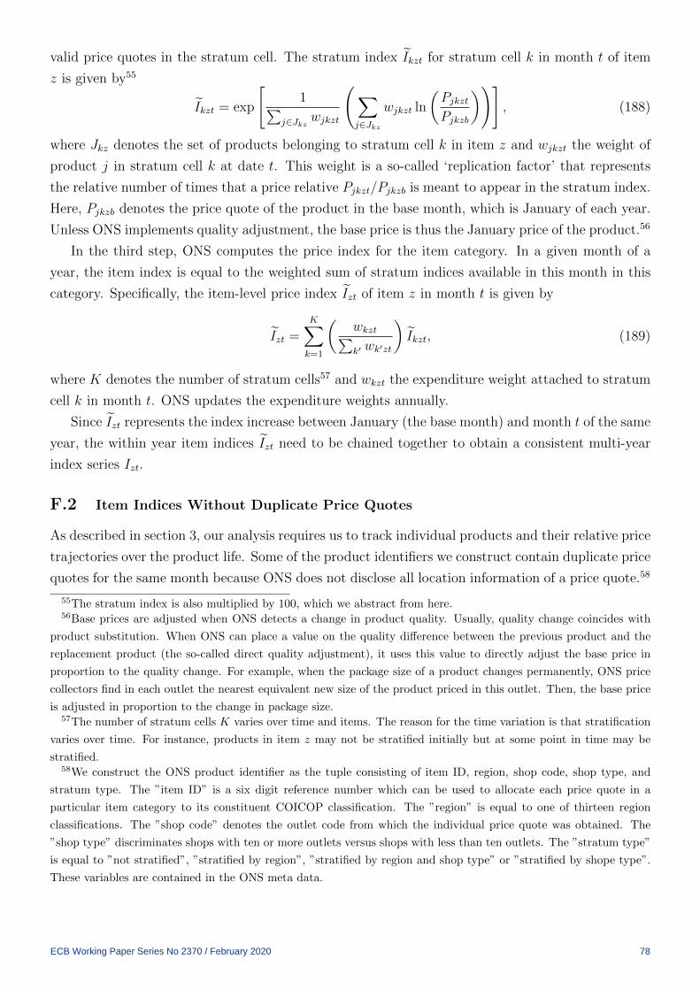
valid price quotes in the stratum cell. The stratum index Ikzt for stratum cell k in month t of item

z is given by55

Ikzt = exp

[1∑

j∈Jkz wjkzt

(∑j∈Jkz

wjkzt ln

(PjkztPjkzb

))], (188)

where Jkz denotes the set of products belonging to stratum cell k in item z and wjkzt the weight of

product j in stratum cell k at date t. This weight is a so-called ‘replication factor’ that represents

the relative number of times that a price relative Pjkzt/Pjkzb is meant to appear in the stratum index.

Here, Pjkzb denotes the price quote of the product in the base month, which is January of each year.

Unless ONS implements quality adjustment, the base price is thus the January price of the product.56

In the third step, ONS computes the price index for the item category. In a given month of a

year, the item index is equal to the weighted sum of stratum indices available in this month in this

category. Specifically, the item-level price index Izt of item z in month t is given by

Izt =K∑k=1

(wkzt∑k′ wk′zt

)Ikzt, (189)

where K denotes the number of stratum cells57 and wkzt the expenditure weight attached to stratum

cell k in month t. ONS updates the expenditure weights annually.

Since Izt represents the index increase between January (the base month) and month t of the same

year, the within year item indices Izt need to be chained together to obtain a consistent multi-year

index series Izt.

F.2 Item Indices Without Duplicate Price Quotes

As described in section 3, our analysis requires us to track individual products and their relative price

trajectories over the product life. Some of the product identifiers we construct contain duplicate price

quotes for the same month because ONS does not disclose all location information of a price quote.58

55The stratum index is also multiplied by 100, which we abstract from here.56Base prices are adjusted when ONS detects a change in product quality. Usually, quality change coincides with

product substitution. When ONS can place a value on the quality difference between the previous product and the

replacement product (the so-called direct quality adjustment), it uses this value to directly adjust the base price in

proportion to the quality change. For example, when the package size of a product changes permanently, ONS price

collectors find in each outlet the nearest equivalent new size of the product priced in this outlet. Then, the base price

is adjusted in proportion to the change in package size.57The number of stratum cells K varies over time and items. The reason for the time variation is that stratification

varies over time. For instance, products in item z may not be stratified initially but at some point in time may be

stratified.58We construct the ONS product identifier as the tuple consisting of item ID, region, shop code, shop type, and

stratum type. The ”item ID” is a six digit reference number which can be used to allocate each price quote in a

particular item category to its constituent COICOP classification. The ”region” is equal to one of thirteen region

classifications. The ”shop code” denotes the outlet code from which the individual price quote was obtained. The

”shop type” discriminates shops with ten or more outlets versus shops with less than ten outlets. The ”stratum type”

is equal to ”not stratified”, ”stratified by region”, ”stratified by region and shop type” or ”stratified by shope type”.

These variables are contained in the ONS meta data.


For our analysis, we discard all price quotes belonging to the product identifiers with duplicate price

quotes.

When then recompute item indices using official ONS methodology (see appendix F.1), discarding

products with duplicate price quotes, and compare the recomputed item indices with the official ONS

item indices.

We consider a recomputed item index as sufficiently accurate, whenever the root mean squared

error (RMSE) of the log difference between the recomputed and the official index is below 2%,

RMSEz =

√1

Tz

∑Tz

[ln(IOzt

)− ln

(Izt

)]2 < 0.02,

where IOzt denotes the official ONS index of item category z in month t, Izt the recomputed item

index and Tz the sample period for which both indices display non-missing values. We also require

that recomputed item indices do not display temporarily missing values. We find that 1093 of the

1233 item categories fulfill these requirements.59 These 1093 item categories constitute our baseline

sample.

Panel A in figure 12 depicts the distribution of RMSEs for all 1233 item categories. RMSEs are

generally low: the median (mean) error is equal to 0.006 (0.0079). Pairwise correlations between

recomputed and official ONS item indices in Panel B typically exceed 0.95 and the median (mean)

correlation is equal to 0.984 (0.972).60 Panel C in figure 12 depicts the RMSE (the upward-sloping

line) and the correlations for all items with an RMSE<0.02. It shows that for the vast majority of

items that satisfy RMSE<0.02, we have a high correlation (above 0.9). Only few items display a

somewhat lower correlation.

Figure 13 further illustrates the properties of the 1093 recomputed item indices in our baseline

sample. Panel A shows that the numbers of recomputed and ONS item indices evolve in parallel and

tend to both increase over the sample period. For the item categories in our baseline sample, the

implied annual entry and exit rates are equal to 6.02% and 5.37%, respectively, which indicates fairly

modest turnover at the item category level.61 Furthermore, only about half of the 1093 recomputed

item indices are present in the average year (503 out of 1093). The same pattern is present when

considering all ONS item indices for which micro price data is available (675 out of 1233). Panel B

reports the relative number and the expenditure share of items in our baseline sample relative to the

59In particular, 68 of the recomputed indices do not fulfill the RMSE criterion. Another 72 of the recomputed item

indices fulfill the RMSE criterion but display temporarily missing values. We exclude these indices, which often refer

to seasonal products for which prices are missing in certain months in each year, to avoid complications when chaining

item indices with missing values in the month of January.60Correlations are meaningful statistics because at this stage of the analysis, the base period of item indices corre-

sponds to the month of January in the current year.61The entry rate is the share of item categories newly introduced in the current year, relative to all item categories

present in this year. The exit rate is the share of item categories present in the previous year but no longer present

in this year. Item turnover primarily reflects decisions taken at ONS, which are often determined by methodological

changes or data production requirements such as keeping the number of items in the basket roughly steady over time.


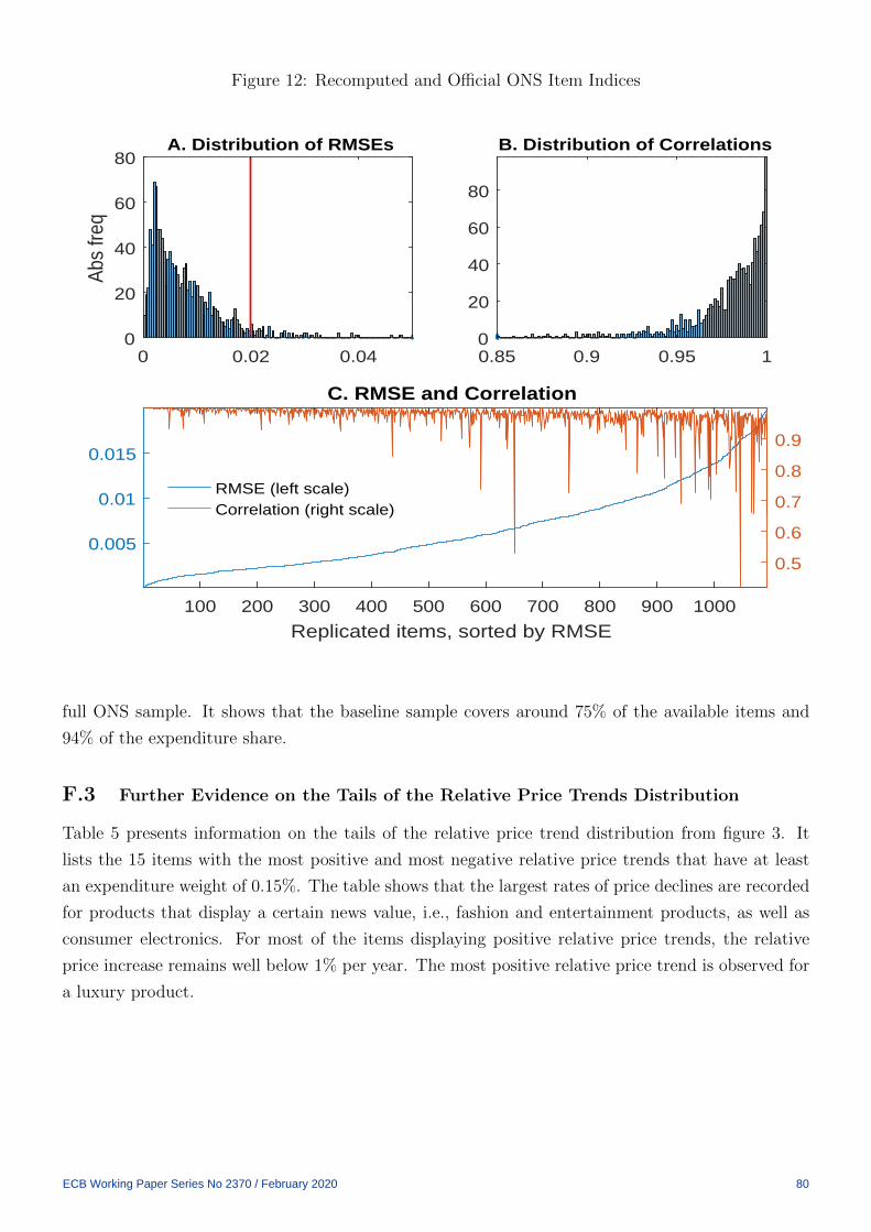
Figure 12: Recomputed and Official ONS Item Indices

A. Distribution of RMSEs

0 0.02 0.040

20

40

60

80

Abs

freq

B. Distribution of Correlations

0.85 0.9 0.95 10

20

40

60

80

100 200 300 400 500 600 700 800 900 1000

Replicated items, sorted by RMSE

0.005

0.01

0.015

0.5

0.6

0.7

0.8

0.9

C. RMSE and Correlation

RMSE (left scale)Correlation (right scale)

full ONS sample. It shows that the baseline sample covers around 75% of the available items and

94% of the expenditure share.

F.3 Further Evidence on the Tails of the Relative Price Trends Distribution

Table 5 presents information on the tails of the relative price trend distribution from figure 3. It

lists the 15 items with the most positive and most negative relative price trends that have at least

an expenditure weight of 0.15%. The table shows that the largest rates of price declines are recorded

for products that display a certain news value, i.e., fashion and entertainment products, as well as

consumer electronics. For most of the items displaying positive relative price trends, the relative

price increase remains well below 1% per year. The most positive relative price trend is observed for

a luxury product.


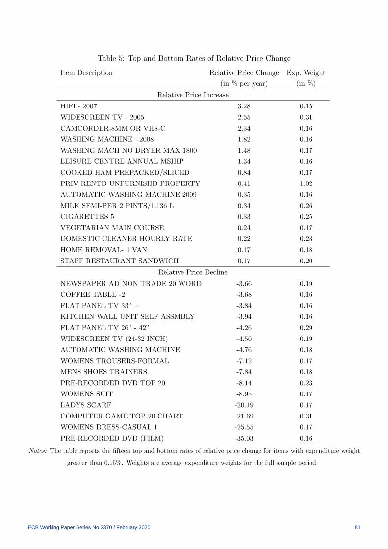
Table 5: Top and Bottom Rates of Relative Price Change

Item Description Relative Price Change Exp. Weight

(in % per year) (in %)

Relative Price Increase

HIFI - 2007 3.28 0.15

WIDESCREEN TV - 2005 2.55 0.31

CAMCORDER-8MM OR VHS-C 2.34 0.16

WASHING MACHINE - 2008 1.82 0.16

WASHING MACH NO DRYER MAX 1800 1.48 0.17

LEISURE CENTRE ANNUAL MSHIP 1.34 0.16

COOKED HAM PREPACKED/SLICED 0.84 0.17

PRIV RENTD UNFURNISHD PROPERTY 0.41 1.02

AUTOMATIC WASHING MACHINE 2009 0.35 0.16

MILK SEMI-PER 2 PINTS/1.136 L 0.34 0.26

CIGARETTES 5 0.33 0.25

VEGETARIAN MAIN COURSE 0.24 0.17

DOMESTIC CLEANER HOURLY RATE 0.22 0.23

HOME REMOVAL- 1 VAN 0.17 0.18

STAFF RESTAURANT SANDWICH 0.17 0.20

Relative Price Decline

NEWSPAPER AD NON TRADE 20 WORD -3.66 0.19

COFFEE TABLE -2 -3.68 0.16

FLAT PANEL TV 33” + -3.84 0.16

KITCHEN WALL UNIT SELF ASSMBLY -3.94 0.16

FLAT PANEL TV 26” - 42” -4.26 0.29

WIDESCREEN TV (24-32 INCH) -4.50 0.19

AUTOMATIC WASHING MACHINE -4.76 0.18

WOMENS TROUSERS-FORMAL -7.12 0.17

MENS SHOES TRAINERS -7.84 0.18

PRE-RECORDED DVD TOP 20 -8.14 0.23

WOMENS SUIT -8.95 0.17

LADYS SCARF -20.19 0.17

COMPUTER GAME TOP 20 CHART -21.69 0.31

WOMENS DRESS-CASUAL 1 -25.55 0.17

PRE-RECORDED DVD (FILM) -35.03 0.16

Notes: The table reports the fifteen top and bottom rates of relative price change for items with expenditure weight

greater than 0.15%. Weights are average expenditure weights for the full sample period.


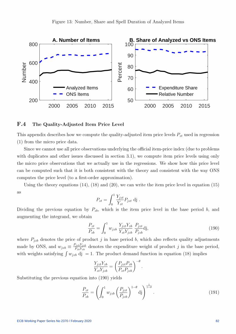
Figure 13: Number, Share and Spell Duration of Analyzed Items

2000 2005 2010 2015200

400

600

800

Num

ber

A. Number of Items

Analyzed ItemsONS Items

2000 2005 2010 201550

60

70

80

90

100

Per

cent

B. Share of Analyzed vs ONS Items

Expenditure ShareRelative Number

C. Spells of Analyzed vs ONS Items

5 10 15 20

Years

0

50

100

150

200

Num

ber

ONS ItemsAnalyzed Items

D. Spells of Analyzed Items

5 10 15 20

Years

0

5

10

15P

erce

ntunweightedweighted

F.4 The Quality-Adjusted Item Price Level

This appendix describes how we compute the quality-adjusted item price levels Pzt used in regression

(1) from the micro price data.

Since we cannot use all price observations underlying the official item-price index (due to problems

with duplicates and other issues discussed in section 3.1), we compute item price levels using only

the micro price observations that we actually use in the regressions. We show how this price level

can be computed such that it is both consistent with the theory and consistent with the way ONS

computes the price level (to a first-order approximation).

Using the theory equations (14), (18) and (20), we can write the item price level in equation (15)

as

Pzt =

∫ 1

0

YjztYzt

Pjzt dj .

Dividing the previous equation by Pzb, which is the item price level in the base period b, and

augmenting the integrand, we obtain

PztPzb

=

∫ 1

0

wjzbYjztYzbYztYjzb

PjztPjzb

dj, (190)

where Pjzb denotes the price of product j in base period b, which also reflects quality adjustments

made by ONS, and wjzb ≡ PjzbYjzbPzbYzb

denotes the expenditure weight of product j in the base period,

with weights satisfying∫wjzb dj = 1. The product demand function in equation (18) implies

YjztYzbYztYjzb

=

(PjztPzbPztPjzb

)−θ.

Substituting the previous equation into (190) yields

PztPzb

=

(∫ 1

0

wjzb

(PjztPjzb

)1−θ

dj

) 11−θ

. (191)


Linearizing the previous equation around Pjzt/Pjzb = 1 delivers

PztPzb

=

∫ 1

0

wjzbPjztPjzb

dj +O(2). (192)

The advantage of the linearized model-consistent equation (192) is that it does not depend on the

demand elasticity θ showing up in the non-linear expression (191).

Linearizing the ONS stratum price index in equation (188) around Pjkzt/Pjkzb = 1 delivers

Ikzt =∑j∈Jkz

wjkztPjkztPjkzb

+O(2),

where wjkzt ≡ wjkzt/(∑

j′∈Jkz wj′kzt

). Using the ONS approach to aggretate stratum indices to item

indices, see equation (189), we obtain from the previous equation

Izt =K∑k=1

((wkzt∑k wkzt

) ∑j∈Jkz

wjkztPjkztPjkzb

)+O(2). (193)

This shows that the ONS approach (193) and the theory-consistent approach (192) deliver to first

order the same price index, provided we set the product weight in equation (192) equal to

wjzb =

(wkzt∑k′ wk′zt

)wjkzt,

where k denotes the stratum to which product j belongs. Using the previous weights we compute

the quality-adjusted item price level. Following ONS, we then chain the index growth rates across

years to get the multi-year series for the price index at the item level.


Acknowledgements We thank our discussants Yuriy Gorodnichenko, Volker Hahn, Martin Seneca, and Alexander Wolman for excellent discussions. We also thank Andrey Alexandrov, seminar participants at the Dutch Central Bank (DNB), Federal Reserve Bank of New York, Goethe University in Frankfurt, University of Oxford, the 2019 ASSA Annual Meeting in Atlanta, the 2019 Inflation Conference at the Federal Reserve Bank of Cleveland, the Society for Economic Dynamics Meeting 2019, St. Louis, the CESifo Area Conference on Macro, Money and International Finance, 2019, and the ECB Monetary Policy Conference 2019 for comments and suggestions. Special thanks go to our research assistant Michal Marencak. The contribution by Klaus Adam has been supported by CRC-TR224 of the German Research Foundation. The opinions expressed in this paper are those of the authors and do not necessarily reflect the views of the ECB, the Deutsche Bundesbank or the Eurosystem. Klaus Adam University of Oxford, Oxford, United Kingdom; CEPR; email: [email protected] Henning Weber Deutsche Bundesbank, Frankfurt am Main, Germany; email: [email protected]

© European Central Bank, 2020

Postal address 60640 Frankfurt am Main, Germany Telephone +49 69 1344 0 Website www.ecb.europa.eu

All rights reserved. Any reproduction, publication and reprint in the form of a different publication, whether printed or produced electronically, in whole or in part, is permitted only with the explicit written authorisation of the ECB or the authors.

This paper can be downloaded without charge from www.ecb.europa.eu, from the Social Science Research Network electronic library or from RePEc: Research Papers in Economics. Information on all of the papers published in the ECB Working Paper Series can be found on the ECB’s website.

PDF ISBN 978-92-899-4013-9 ISSN 1725-2806 doi:10.2866/453066 QB-AR-20-022-EN-N

mailto:[email protected]

mailto:[email protected]

http://www.ecb.europa.eu/

http://www.ecb.europa.eu/

http://ssrn.com/

https://ideas.repec.org/s/ecb/ecbwps.html

http://www.ecb.europa.eu/pub/research/working-papers/html/index.en.html

Working Paper Series · We start by showing that sticky price models imply that the documented...

Documents

Transcript of Working Paper Series · We start by showing that sticky price models imply that the documented...