WORKING PAPER SERIES - ecb.europa.eu · THE ROLE OF REAL WAGE RIGIDITY AND LABOR ... and Andrew...

WORKING PAPER SER IESNO. 556 / NOVEMBER 2005

THE ROLE OF REAL WAGE RIGIDITY AND LABOR MARKETFRICTIONS FOR UNEMPLOYMENT AND INFLATION DYNAMICS

by Kai Christoffel and Tobias Linzert

EUROSYSTEM INFLATION PERSISTENCE NETWORK

In 2005 all ECB publications will feature

a motif taken from the

€50 banknote.

WORK ING PAPER S ER I E SNO. 556 / NOVEMBER 2005

This paper can be downloaded without charge from http://www.ecb.int or from the Social Science Research Network

electronic library at http://ssrn.com/abstract_id=850884.

THE ROLE OF REAL WAGE RIGIDITY

AND LABOR MARKETFRICTIONS FOR

UNEMPLOYMENT AND INFLATION DYNAMICS 1

by Kai Christoffel 2

and Tobias Linzert 3

EUROSYSTEM INFLATION PERSISTENCE NETWORK

1 We thank Heinz Herrmann, Andrew Levin, Michael Krause, Keith Küster and an anonymous referee for helpful comments andsuggestions.We are also grateful to the seminar participants at the Goethe-University Frankfurt and the Deutsche Bundesbank

and the members of the Eurosystem’s Inflation Persistence Network for their suggestions.The research was undertaken while both authors were affiliated with the Deutsche Bundesbank and the Goethe University Frankfurt.The views expressed in

this paper are those of the authors and do not necessarily reflect those of the ECB or Bundesbank.2 Corresponding address: European Central Bank, Kaiserstrasse 29, 60311 Frankfurt, Germany;

e-mail: [email protected] 3 European Central Bank, Kaiserstrasse 29, 60311 Frankfurt, Germany;

e-mail:[email protected]

© European Central Bank, 2005

AddressKaiserstrasse 2960311 Frankfurt am Main, Germany

Postal addressPostfach 16 03 1960066 Frankfurt am Main, Germany

Telephone+49 69 1344 0

Internethttp://www.ecb.int

Fax+49 69 1344 6000

Telex411 144 ecb d

All rights reserved.

Any reproduction, publication andreprint in the form of a differentpublication, whether printed orproduced electronically, in whole or inpart, is permitted only with the explicitwritten authorisation of the ECB or theauthor(s).

The views expressed in this paper do notnecessarily reflect those of the EuropeanCentral Bank.

The statement of purpose for the ECBWorking Paper Series is available fromthe ECB website, http://www.ecb.int.

ISSN 1561-0810 (print)ISSN 1725-2806 (online)

The Eurosystem Inflation Persistence Network

This paper reflects research conducted within the Inflation Persistence Network (IPN), a

team of Eurosystem economists undertaking joint research on inflation persistence in the

euro area and in its member countries. The research of the IPN combines theoretical and

empirical analyses using three data sources: individual consumer and producer prices;

surveys on firms’ price-setting practices; aggregated sectoral, national and area-wide

price indices. Patterns, causes and policy implications of inflation persistence are

addressed.

Since June 2005 the IPN is chaired by Frank Smets; Stephen Cecchetti (Brandeis

University), Jordi Galí (CREI, Universitat Pompeu Fabra) and Andrew Levin (Board of

Governors of the Federal Reserve System) act as external consultants and Gonzalo

Camba-Méndez as Secretary.

The refereeing process is co-ordinated by a team composed of Günter Coenen

(Chairman), Stephen Cecchetti, Silvia Fabiani, Jordi Galí, Andrew Levin, and Gonzalo

Camba-Méndez. The paper is released in order to make the results of IPN research

generally available, in preliminary form, to encourage comments and suggestions prior to

final publication. The views expressed in the paper are the author’s own and do not

necessarily reflect those of the Eurosystem.

3ECB

Working Paper Series No. 556November 2005

CONTENTS

Abstract 4

Non-technical summary 5

1 Introduction 7

2 The business cycle model with labormarket matching 9

2.1 Household problem 10

2.2 Job matching 10

2.2.1 Job destruction 12

2.2.2 Job creation 13

2.3 Wage setting 14

2.3.1 Efficient Nash bargaining 15

2.3.2 Right-to-manage bargaining 16

2.3.3 Introducing wage rigidity 17

2.4 Final good firms and price setting 19

2.5 Monetary policy 20

3 Impact of real wage rigidity 21

3.1 Efficient bargaining setup 21

3.2 Right-to-manage bargaining setup 22

4 The impact of labor market fundamentals 24

4.1 Bargaining power of workers 25

4.2 Employment protection 26

Conclusions 27

References 29

Appendix 33

European Central Bank working paper series 38

Abstract

In this paper we incorporate a labor market with matching frictions and wagerigidities into the New Keynesian business cycle model. In particular, we analyzethe effect of a monetary policy shock and investigate how labor market frictionsaffect the transmission process of monetary policy. The model allows real wagerigidities to interact with adjustments in employment and hours affecting inflationdynamics via marginal costs. We find that the response of unemployment andinflation to an interest rate innovation depends on the degree of wage rigidity.Generally, more rigid wages translate into more persistent movements of aggregateinflation. Moreover, the impact of a monetary policy shock on unemployment andinflation depends also on labor market fundamentals such as bargaining power andthe flows in and out of employment.

Keywords: Monetary Policy, Matching Models, Labor Market Search, Inflation Per-sistence, Real Wage RigidityJEL classification: E52, J64, E32, E31

4ECBWorking Paper Series No. 556November 2005

Non-technical Summary

Europe’s labor markets are characterized by firing costs, generous unemploymentbenefits and strong unions that are perceived to contribute to sluggish labor mar-ket adjustments. Moreover, the collective wage bargaining process is seen to pre-vent wages from adjusting instantaneously, introducing a substantial degree of wagerigidity. Therefore, rigidities and frictions in the labor market might be crucial forunderstanding sluggishness in firms’ marginal cost and their price setting behavior.

In this paper, we stress the role of the labor market in determining firms’ marginalcost and link labor market adjustments directly to the dynamics of inflation. Forthat reason, we introduce a labor market model with matching frictions into the NewKeynesian business cycle framework. We particularly introduce a model with right-to-manage wage bargaining to incorporate a real wage rigidity in form of a social wagenorm which has important implications for the joint dynamics of unemployment andinflation in our New Keynesian DSGE model.

The traditional New Keynesian dynamic stochastic general equilibrium model of busi-ness cycle fluctuations generally fails to account for the degree of inflation persistenceobserved in actual data. Therefore, we specifically explore the question whether theunderlying labor market regime contributes to explaining inflation persistence. Inparticular, we analyze how different degrees of real wage rigidities affect the reactionof unemployment and inflation to a shock in monetary policy under different wagebargaining regimes. Moreover, we study the impact of a monetary policy shock onunemployment and inflation conditional on labor market fundamentals such as bar-gaining power of the workers and the flows in and out of employment.

We find that rigid real wages contribute to explaining persistent inflation. Employinga right-to-manage bargaining framework, wages feed directly into firm’s marginal costand hence into inflation dynamics via the New Keynesian Phillips curve. Introducinga real wage rigidity in form of a social wage norm, we can show that more rigidwages translate into more persistent movements of aggregate inflation. In contrast,the channel from wages to inflation is missing under the assumption of an efficientbargaining model and, therefore, fails to generate inflation persistence.

Our calibration also shows that unemployment and inflation dynamics do not onlydepend on rigid wages but also on the parameters that determine employment pro-tection and bargaining power of workers. Generally, ”institutional” parameters thatraise the volatility in wages, increase also the response of inflation and tend to reduceits persistence. On the other hand, anything that spurs the volatility in labor flows,dampens the adjustments of wages and, therefore, tends to increase the persistence ininflation.

The model reveals that the labor market has important implications for the trans-mission process of monetary policy. The inclusion of a labor market into the NewKeynesian model introduces another channel along which real and nominal rigiditiescan be incorporated into the model. The ”labor market channel” significantly affectsthe dynamics of employment and inflation. In particular, real wage rigidity appearsto play a key role in shaping marginal cost dynamics and, consequently persistent

5ECB


movement in inflation rates. Our model suggests that the central bank may benefitfrom closely monitoring the labor market. From the developments in real labor flowsas well as real wage movements the central bank can infer on the dynamics and par-ticularly, on the degree of persistence of the inflation rate. Therefore, differences inlabor market regimes may help to explain inflation dynamics across countries.


1 Introduction

Europe’s labor markets are rigid in many respects. High firing costs, generous un-

employment benefits and strong unions are perceived to contribute to sluggish labor

market adjustments. Moreover, the collective wage bargaining process is seen to pre-

vent wages from adjusting instantaneously, introducing a substantial degree of wage

rigidity. Therefore, rigidities and frictions in the labor market might be crucial for

understanding sluggishness in firms’ marginal cost and their price setting behavior.

In this paper, we stress the role of the labor market in determining firms’ marginal

cost and link labor market adjustments directly to the dynamics of inflation. For

that reason, we introduce a Mortensen and Pissarides (1994) labor market model

with matching frictions into the New Keynesian business cycle framework, see also

Walsh (2003) and Trigari (2003). We particularly extend the Trigari (2003) model

with right-to-manage wage bargaining to incorporate a real wage rigidity in form of a

Hall (2005) type wage norm. In contrast to the traditional Nash efficient bargaining,

the right-to-manage bargaining constitutes a channel through which wages affect the

marginal costs of firms. Since marginal costs feed into the determination of prices

through the New Keynesian Phillips curve, we establish a direct channel of real wage

rigidities to translate into aggregate inflation.

We specifically explore the question whether the underlying labor market regime con-

tributes to explaining inflation persistence. In particular, we analyze how different

degrees of real wage rigidity affect the reaction of unemployment and inflation to a

shock in monetary policy under different wage bargaining regimes. Moreover, we study

the impact of a monetary policy shock on unemployment and inflation conditional on

labor market fundamentals such as bargaining power of the workers and the flows in

and out of employment.

The lack of inflation persistence implied by the standard New Keynesian model has

triggered a line of research focusing on firms’ price setting process. Generally, this

approach accounts for the observed persistence only if a substantial backward-looking

component is included into the Phillips curve relation, see Fuhrer and Moore (1995),

Gali and Gertler (1999) and Christiano, Eichenbaum, and Evans (2005). A second line

of research focuses on inflation persistence stemming from inertia in the underlying

process of marginal costs. Erceg, Henderson, and Levin (2000) introduce Calvo type

7ECB


nominal wage rigidities to generate marginal cost sluggishness. Indeed, Gali, Gertler,

and Lopez-Salido (2001) find that wage rigidities are a significant factor driving the

persistent movement in marginal cost for both the euro area and the U.S..1

Yet, the mere modelling of wage rigidities might not suffice to fully understand the

factors behind sluggish marginal cost. Adjustments in the labor market take place on

the hours of work as well as the employment margin. Besides, in light of high levels

of unemployment in Europe and generally rigid labor markets a cleared labor market

neglecting unemployment might be a misleading assumption. In contrast, our model

incorporates matching frictions that generate equilibrium unemployment. Moreover,

workers and firms bargain over wages in a collective wage bargaining manner. In

addition to adjustments in hours of work per worker, the model provides an additional

adjustment channel via the employment margin. Consequently, we employ a model

with nominal price rigidities that incorporates both real wage rigidities and matching

frictions in the labor market. This model framework will allow us to analyze how labor

market dynamics and particularly the adjustment of wages translate into marginal cost

and inflation dynamics.

Our main results can be summarized as follows. Our model features a ”labor market

channel” in the monetary transmission mechanism. We can show that the interaction

of the specific wage setting process, i.e. the right-to-manage bargaining with real wage

rigidities establish a direct channel on aggregate inflation dynamics. In particular,

assuming a high degree of wage rigidity induces marginal cost to adjust slowly which

translates into more persistent inflation dynamics. In contrast, using an efficient bar-

gaining framework, in which marginal cost are mainly determined by hours worked not

wages, the wage rigidity does not lead to higher inflation persistence, see also Krause

and Lubik (2003). Moreover, our calibration shows that unemployment and inflation

dynamics depend also on the parameters that determine employment protection and

bargaining power of workers. And finally, the model is able to describe both the effect

of a monetary policy shock on unemployment and on inflation. An adverse monetary

policy shock in our model leads to a negative response of unemployment and inflation,

displaying the traditional Phillips curve trade-off.

The understanding of labor markets for the transmission process might be of crucial

1 See Christiano, Eichenbaum, and Evans (2005) and Edge, Laubach, and Williams (2003) whoalso stress the importance of wage rigidities contributing critically to explain inflation and outputdynamics.


importance for a central bank. First, inflation dynamics and hence inflationary pres-

sures might depend on the flexibility of wages and labor flows. Second, countries that

differ with respect to their labor market regime might respond quite differently to a

monetary policy shock. In general, understanding labor market adjustments and how

they are related to the monetary transmission process may reduce the uncertainty

associated with the reaction of inflation to a monetary policy action.

The remainder of the paper is structured as follows. Section 2 introduces the business

cycle model featuring nominal price and real wage rigidities. In Section 3 we analyze

the role of wage rigidities for inflation dynamics in our simulated model framework.

Section 4 assesses the impact of labor market fundamentals on inflation dynamics.

Section 5 offers some conclusions and provides an outlook for further research.

2 The Business Cycle Model with Labor Market Match-

ing

Following Trigari (2003), we introduce a New Keynesian style business cycle model

incorporating labor market frictions. These labor market frictions are twofold. First,

we use the standard Mortensen-Pissarides model to account for equilibrium unem-

ployment. This imposes a real rigidity on the adjustment of the factors of production

to aggregate shocks. Second, we follow Hall (2005) and Krause and Lubik (2003) by

including real wage rigidity in form of a wage norm. In that sense we extend the

model by Trigari (2003) to allow for rigidities in wage contracts.

The model structure is characterized by a separation between firms in the wholesale

and retail market. The intermediate goods are produced by competitive firms in

the wholesale sector employing labor as the only input to production. The retail

sector firms buy wholesale goods at marginal cost, transform them into differentiated

goods and sell them with a mark-up over marginal cost in a monopolistic competitive

environment, see Walsh (2003).2

2 The two market structure of wholesale and retail sector simplifies the structure of the model.Notice that Krause and Lubik (2003) embed the two sector structure into a single integrated firmemploying labor to produce intermediate and final good.

9ECB


2.1 Household Problem

There is a continuum of households on the interval [0, 1]. The representative household

chooses {ct, ht}∞

t=1 to maximize its utility given by:

max Et

∞∑

t=0

βt

[c1−σt

1 − σ− κh

h1+φt

1 + φ

](1)

where the first term is the utility from consuming ct of the final good while the second

part represents the disutility from work by supplying ht units of hours. The degree

of risk aversion is given by σ and φ denotes the inverse of the intertemporal elasticity

of substitution of labor. κh accounts for the relative importance of disutility of work

and utility from consumption in total utility.

Households maximize consumption subject to the following budget constraint:

ct +Bt

ptrnt

= dt +Bt−1

pt(2)

where pt is the aggregate price level, Bt is per capita holdings of one period risk free

bond, rnt is the gross nominal interest rate on this bond and dt denotes the per capita

income of the household in period t.

Household members can be employed or unemployed. When employed they receive

the wage payments wtht, when unemployed they engage in home production of a non-

tradable goods or receive unemployment benefits which are evaluated in consumption

units, bt. In the absence of perfect income insurance an individual’s savings decision

would depend on its employment history and prospects. To avoid any distributional

issues that may arise from this instance, we follow Merz (1995) and Andolfatto (1996)

in assuming that households pool their income and consumption. Conditional on this

assumption households optimality conditions can be given by the usual intra- and

intertemporal relation.

2.2 Job Matching

In the following section we lay out the search and matching model of Mortensen-

Pissarides that is incorporated into a New Keynesian style business cycle model to

explicitly model labor market frictions in the form of equilibrium unemployment, see

Mortensen and Pissarides (1994), Mortensen and Pissarides (1999), Pissarides (2000).


Trade in the labor market is an uncoordinated, time consuming, and costly activity

that introduces frictions which lead to imperfect outcomes in the labor market. Jobs

are constantly created and destroyed and unemployed workers look for new jobs gen-

erating unemployment in equilibrium. The process through which workers and firms

find each other is represented by a matching function accounting for the imperfections

and transaction cost in the labor market.3 This function summarizes the entire search

process in a single relation where the number of matches is a function of the number

of unemployed persons, ut, and the number of vacant jobs, vt, in the labor market:

mt = m(ut, vt) = mut v

1−t (3)

with being the elasticity of the matching with respect to the stock of unemployed

persons. The parameter m captures all factors that influence the efficiency of match-

ing. The function is assumed to have constant returns to scale.

The probability that a vacant job is matched with a worker is:

qt =mt

vt= mθ−

t (4)

where θt = vt

utdefines an indicator for the tightness in the labor market. An increase

in the number of vacancies relative to unemployment, θt, reduces the probability that

a vacancy will be filled. This in turn means that additional vacancies per unemployed

worker imply an increase of the probability that the unemployed person finds a job.

Accordingly, the corresponding probability for an unemployed worker to find a job is

given by:

st = mt/ut = mθ1−t (5)

where the exit rate from unemployment is an increasing function of the labor market

tightness. For a given number of unemployed persons in the market, the probability

of finding a job increases when the number of vacancies rise.

The probabilities of filling a job and finding a job show that the matching model

introduces two kinds of externalities responsible for determining equilibrium unem-

ployment in the model: the congestion and the labor market tightness externality.

Each firm posting a vacancy creates a negative congestion externality for other firms

3 Frictions usually derive from a complex set of factors such as imperfect information, heterogeneity,absence of perfect insurance, etc. The matching function incorporates the equilibrium outcome ofsuch frictions without the explicit reference to the above sources of frictions.

11ECB


since an additional vacancy decreases the chance for other firms to fill their vacancies.

Conversely, the labor market tightness describes the effect that each additional job

searcher creates a negative search externality for other searchers. Thus, there will be

a stochastic rationing in the labor market which cannot be solved by the usual price

mechanism. The variable, θt, defined to capture both externalities, plays a crucial

role in determining the degree of rationing and hence the equilibrium unemployment

in the labor market.

Once a worker and a firm are matched, they produce output according to the produc-

tion function:

f(ht) = zthαt (6)

where labor, i.e. the number of hours, ht, is the only input to production and zt

represents technological progress.

It is assumed that firms produce the output necessary to provide the aggregate house-

hold demand.

ct = (1 − ρ)ntzthαt (7)

2.2.1 Job Destruction

Unemployment rises after an adverse shock. According to Hall (2004) employed work-

ers do not loose jobs more frequently in a recession than in other times, i.e. job

destruction remains rather constant over time. On the other hand, employers are far

more reluctant to create jobs in a recession. Hence, unemployment rises because the

exit rate of unemployment is lower, and not because the entrance rate is higher.

Therefore, without loss of plausibility, we can assume that job destruction occurs

exogenously at the rate ρ. The rate ρ indicates the proportion of existing matches that

disappear at the beginning of each period, i.e. become unproductive for unspecified

reasons resulting in firms terminating the job.

The number of employed workers at the beginning of each period (nt) evolves as

follows:

nt = (1 − ρ)nt−1 + mt−1 (8)


where the first part of the right hand side represents the matches that survived the

job destruction process in the previous period and the second part being the matches

formed in the previous period which become productive in the current period. It is

important to note the nt gives the number of employed workers at the beginning of

period t. The number of productive workers in period t is therefore given by (1−ρ)nt.

The number of searching workers is given accordingly as (where total labor force is

normalized to one):4

ut = 1 − (1 − ρ)nt (9)

2.2.2 Job Creation

Firms create a job vacancy when the expected gains from an employment relation

exceed the cost of vacancy posting. Until the value of a new job is equal to the cost

of creating a job new firms will enter the market to create vacancies. For simplicity

it is assumed that each firm has one job so vacancy posting and hence the number of

jobs created is a matter of how many firms are in the market.

The value of a job for a firm is given by the contemporaneous payoff and the discounted

future value of the job at the end of the period.

Jt = xtf(ht) − wtht + Et βt+1(1 − ρ)Jt+1 (10)

where xt is the relative price of the intermediate good and wt is the wage the firm

has to pay for an hour of work. Since all the intermediate good producers act in a

competitive environment the relative price is given by marginal cost in relation to the

price of the consumption good. The discount factor is constructed in terms of relative

marginal utility (λt = ∂Ut

∂ct) from consumption, such that βt+s = βsλt+s

λt.

The value of an open vacancy to a firm is given by:

Vt = −κ

λt+ Et βt+1 [qt(1 − ρ)Jt+1 + (1 − qt)Vt+1] (11)

with κ being the utility cost of vacancy posting.5 When a job is vacant, the profit

is zero. Hence the value of a vacancy is determined by the current cost of holding a

4 Note that ut gives the number of searching workers, while the number of unemployed workers atthe beginning of each period is given by 1 − nt.

5 Notice that the vacancy costs cannot just be seen as the pure costs of hiring but also costs formachines and other capital that will be idle while the vacancy is not filled.

13ECB


vacancy open and the expected utility arising from future matches. As long as the

value of a vacancy is greater than zero vacancies are created until Vt = 0.

Taking the difference between the two equations Jt and Vt yields the surplus, Jt − Vt,

to the firm of filling a vacancy. It can be seen from the equations for Jt and Vt that

the value of a firm from a filled vacancy increases in the search cost, the separation

rate, the discount rate and the expected length of search.

Turning to the problem of the worker, we assume that a worker can either be employed

or unemployed. The value of being employed is given by:6

Wt = wtht −g(ht)

λt+ Et βt+1 [(1 − ρ)Wt+1 + ρUt+1] (12)

The first term in the equation is the worker’s wage income. The second term represents

the disutility of work and the last term reflects the future utility of an employment

relation. With a probability ρ the job is destroyed and the worker receives the utility

of being unemployed while the value of being employed is realized if the job remains

productive.

In the same way we can express the value of being unemployed:

Ut = b + Et βt+1 [st(1 − ρ)Wt+1 + (1 − st + stρ)Ut+1] (13)

The value of being unemployed is determined by the value of home production or

unemployment benefits, b, and the probability of finding a job in period t and not

loosing the job at beginning of period t + 1 given by st(1 − ρ). With probability

1 − st(1 − ρ) unemployed workers remain in the unemployment pool, either by being

not matched at all or being matched and separated immediately at the beginning of

the next period.

Taking the difference between the two equations Wt and Ut yields the surplus, Wt−Ut,

to the worker of staying employed. The surplus depends crucially on the level of

unemployment benefits and the tightness in the labor market.

2.3 Wage Setting

In a frictionless Walrasian labor market, hours are chosen to equate the marginal rate

of substitution between leisure and consumption with the marginal product of labor.

6 Where g(ht) = κhh1+φt

1+φdenotes the disutility from supplying labor.


The resulting wage rate equals the marginal product of labor. In a labor market with

matching frictions and equilibrium unemployment, however, the worker and the firm

bargain over wages. In general, wages will be bargained to split the positive rent

or match surplus arising from a successful match between the worker and the firm.7

There are several versions of noncooperative bargaining games that are able to solve

the surplus sharing problem. In the following section we will consider the efficient

Nash bargaining to contrast it with the right-to-manage bargaining.

2.3.1 Efficient Nash Bargaining

A plausible way to split the rent between workers and employers is through efficient

Nash bargaining. MacDonald and Solow (1981) proposed a bargaining game in which

bargaining takes place over employment and wages at the same time. In this case,

wages and the number of hours worked are chosen to maximize the joint surplus:

maxw,h

[Wt − Ut]η [Jt − Vt]

1−η (14)

subject to equations (10) to (13).

This implies the following optimality condition:

ηJt = (1 − η)(Wt − Ut) (15)

The wage in this model can be interpreted as a weighted average of the two ”threat”

points of employers and employees, i.e. the marginal product and the reservation wage,

respectively. The stronger the bargaining power of the worker, the closer the wage is

to the marginal product and vice versa. Therefore, the wage has only a distributive

role of the rent from the foregone expected search costs.

The wage relation following from (15) can be written as:

wt = η

(xtmplt

α+

κθt

λtht

)+ (1 − η)

(mrst

1 + φt+

b

ht

)(16)

Notice that in this formulation the wage does not only depend on the marginal rate of

substitution (mrs) as in the frictionless Walrasian market but also on the state of the

labor market, i.e. the value of household production or level of unemployment benefits

7 The rent is generated since it is costly to both workers and employers not to agree over employment.The worker remains unemployed and has to look for another job and similarly the firm faces searchcosts to find another worker.

15ECB


(b), the labor market tightness (θ), etc. In the theoretical model an increased tightness

of the labor market or higher unemployment benefits implies higher negotiated wages.

In the bargaining process wages and hours are determined simultaneously. This im-

plies that hours are chosen in an efficient way according to the following optimality

condition:

mpltxt = mrst (17)

Under efficient bargaining the outcome lies on the contract curve, i.e. the locus of

tangency points of the isoprofit curve of the firm and worker’s indifference curves.

Any change in hours will be accompanied by a change in the wage as well so that any

renegotiation of hours and wages will yield an agreement on the contract curve. Thus,

the correct measure of firms marginal cost is the worker’s marginal rate of substitution

of consumption and leisure rather than the wage.

2.3.2 Right-To-Manage Bargaining

In contrast to efficient Nash bargaining the right-to-manage model proposes that

unions and firms only bargain over wages and that firms subsequently choose the

level of employment, see Nickell and Andrews (1983) and Trigari (2003). The reason-

ing to negotiate wages and the employment level separately is that firms want to adapt

their labor demand if product demand changes. In practise employers are always able

to adjust employment by changing work hours or the workforce. In this view, the

efficient bargaining solution by which every adjustment in working hours is accompa-

nied by a renegotiation of wages seems too restrictive. Besides, a large proportion of

wages in Europe are covered by collective bargaining agreements at the sectoral level,

leaving the individual firm with the optimal decision on the demand for hours only.

Therefore, the right-to-manage model seems to characterize the institutional setup in

Europe better than the efficient bargaining model.

The product of the weighted economic rents of the negotiating parties, i.e. workers

and employers is maximized with respect to wt:

ηδwt Jt = (1 − η)δf

t (Wt − Ut) (18)

where δwt = ∂Wt

∂wtis the marginal contribution of wages to the value of a job to the

worker and δft = ∂Jt

∂wtis the marginal contribution of the wage to the value of a job to


the firm. Using the relations in equations (10)-(13) yield the following wage equation:

wtht = χt(xtzht + fFt ) + (1 − χt)

κhh1+φt

1+φ

λt+ b − fW

(19)

where fFt and fW

t are the future net present values from employment for the firm and

the worker, respectively and

χt =ηδn

t

ηδwt + (1 − η)δf

t

We can rewrite the wage as:

wt = χt

(xtmplt

α+

κθt

λtht

)+ (1 − χt)

(mrs

1 + φt+

b

ht

)(20)

+χt(1 − st)κ

λtqt

(1 −

1 − χt

χt

χt+1

1 − χt+1

)

As in the efficient bargaining case, the wage differs from the competitive wage. The

wage depends on the respective bargaining power of the negotiating parties, the reser-

vation wage and the general tightness of the labor market. In that sense, the institu-

tional framework of the labor market is crucial for the wage setting process.

Once the wage is determined, firms will choose hours to satisfy the relation:

xtmplt = wt (21)

Wages are set through the bargaining process and are taken as given by the firms

when choosing their level of employment. For every additional hour of work the

firm must pay the previously bargained wage. Therefore, in contrast to the efficient

bargaining case, the wage is now a direct determinant of the firm’s marginal cost. The

mechanism through which wages feed into marginal costs is crucial to our model since

it constitutes a direct channel of wages on inflation dynamics via the New Keynesian

Phillips curve.

2.3.3 Introducing Wage Rigidity

Aggregate wages are characterized by a high degree of persistence. Especially in

Europe, sudden and significant shifts in the aggregate wage level are not observed.

Due to collective wage bargaining agreements, wage changes only take place on a quite

17ECB


infrequent basis. Therefore, a wage that can be freely adjusted each period assumes

a degree of wage flexibility that is hardly consistent with actual practises.

Erceg, Henderson, and Levin (2000) and Christiano, Eichenbaum, and Evans (2005)

introduce wage rigidity into the New Keynesian business cycle model by a Calvo type

wage setting scheme. As in final good price setting, firms are randomly chosen to

change their wages while the remaining firms keep wages unchanged. In Europe,

however, most wages are bargained on a sector wide level, are not allowed to fluctuate

freely and once settled remain unchanged for a given period. More importantly, the

Calvo wage rigidity modelling strategy neglects the crucial interdependence of the

wage bargaining process with other labor market issues, like the flows in and out of

employment or the level of unemployment. For that reason we opt for introducing a

wage rigidity into the labor market setting presented in the previous sections.8

Following Hall (2005), we introduce wage rigidity into the model in the form of a

backward looking social norm.9 The possible outcome of the wage bargain lies within

a bargaining set. The bargaining set is bounded by an upper limit denoting the wage

rate (w(u)t ) for which the firms’s surplus from the employment relation is zero. The

wage level for which the worker is indifferent between working and being unemployed

determines the lower wage bound (w(l)t ).10 All wage levels in this bargaining set are

possible solutions of the wage bargain and can be written as a convex combination of

upper and lower bound:

w⋆t = Γtw

(u)t + (1 − Γt)w

(l)t (22)

where Γt is a function of the specific bargaining regime governed by η.

According to Hall (2005) a wage norm or social consensus can be perceived as a rule to

select an equilibrium within the bargaining set. Without going into the details of the

sources of this wage norm, we assume that the actual wage level is given by a weighted

8 Throughout this paper we are using the term wage rigidity to refer to the general property thatreal wages are not adjusting immediately to the desired level. In contrast to this usage Trigari(2003) is using the term wage rigidity for the right-to-manage bargaining approach where wagesare allocative but free to adjust immediately (compare Section 2.3.2).

9 The wage norm has originally been introduced into the matching model to improve the model’sperformance in replicating labor market fluctuations. In particular, the model cannot explain wellthe magnitude of the cyclical behavior of unemployment and vacancies, see e.g. Hall (2005) andShimer (2005). A wage norm limits the adjustment capabilities of wages and hence increases theadjustments on the labor quantity side. This channel substantially increases the business cyclefluctuations of unemployment and vacancies.

10 The upper and the lower limit of the wage bargaining set are derived from the value functionsdefined in equations (10) and (11) respectively (12) and (13).


average of past wage level and the equilibrium wage level defined in Equation (22):11

wt = (1 − δ)w⋆t + δw (23)

where w = wt−1 and δ denoting the respective weight. The wage norm used in this

framework can be seen as encompassing various sources of wage rigidities.12 While

being a short cut to a micro founded wage rigidity, the aggregate wage norm used

in this paper constitutes a plausible starting point for analyzing the impact of wage

rigidities on the monetary transmission process, see also Krause and Lubik (2003),

Uhlig (2004) and Blanchard and Gali (2005), which take a similar approach.

In contrast to the efficient bargaining model, the right-to-manage model of the previous

section establishes a link between the wage setting and firms’ marginal cost. In fact,

in our model the wage rigidity will directly influence the marginal cost process.13 In a

New Keynesian model with a Walrasian labor market an adverse shock to production

usually leads to large declines in real wages. Marginal costs of firms fall accordingly

and the incentive for price adjustments is high. This is, however, in contrast to the

empirical evidence that commonly demonstrates fluctuations of prices and wages to

be rather small. Hence, the departure from the Walrasian labor market with wage

rigidities may improve the model generated dynamics of output and inflation. More

specifically, the introduction of the wage norm depresses marginal cost fluctuations and

helps to generate more persistent inflation dynamics via the New Keynesian Phillips

curve.

2.4 Final Good Firms and Price Setting

The final good firms aggregate the intermediate goods into the final consumption

good.14 The output index is assembled using the standard aggregation technology.

yt =

[∫ 1

0y

ǫ−1ǫ

it

] ǫǫ−1

(24)

11 The wage norm can be rationalized, for example, in terms of an aggregation of individual wagedecisions, each subject to idiosyncratic productivity shocks disturbing the wage outcome. Onlythose wages that fall out of the boundaries of the wage bargaining set are reset to the nearestboundary. In general, the average wage in a period becomes the norm for next period, see Hall(2003) for details.

12 See for example Boeri and Burda (2003) or Danthine and Kurmann (2004) for possible microfoun-dations.

13 Notice that the wage rigidity in this model does not affect the formation of a match itself. However,a wage rigidity influences the vacancy posting of employers as slow moving wages affect the profitcondition and hence the amount of open vacancies posted by firms.

14 This section follows the standard setting described in Rotemberg and Woodford (1998).

19ECB


with yt, yit and ǫ being aggregate output, the individual firm’s output and the firm’s

own price elasticity, respectively. The final good is sold at its unit price defined as

pt =

[∫ 1

0p1−ǫ

it

] 11−ǫ

(25)

The resulting demand for each aggregator depends on the relative price and aggregate

demand.

yit =

(pit

pt

)−ǫ

yt (26)

Following the specification introduced by Calvo (1989) we can write the Dixit-Stiglitz

price index as

pt =[(1 − ϕ)p⋆1−ǫ

t + ϕp1−ǫt−1

] 11−ǫ (27)

where (1 − ϕ) denotes the per period probability that a firm is able to reset its price

to the optimal price p⋆t . The remaining fraction ϕ of firms keep their prices at the

levels prevailed in the previous period. The optimal price p⋆t is chosen to maximize

profits over the expected time span until the firm can re-optimize the price.

Et

∞∑

s=0

ϕsβt+s

[p⋆

it

pt+s− xt+s

]yi,t+s (28)

The solution to this problem is given by

pit =ǫ

ǫ − 1Et

∞∑

s=0

ωt,t+spt+sxt+s (29)

The weights ωt,t+s are given by

ωt,t+s =ϕsβt+sRit,t+s

Et

∑∞

k=0 ϕkβt+kRit,t+k(30)

with Rit denoting the real interest rate.

2.5 Monetary Policy

The central bank’s monetary policy is modelled via a Taylor-type interest rate rule

according to which the nominal interest rate evolves as:

rnt = (rn

t−1)ρm

Et(pt+1/pt)γπ(1−ρm)(yt)

γy(1−ρm)eǫmt (31)


3 Impact of Real Wage Rigidity

To solve the model described in the previous section the equations are linearized

around the model’s steady state. The resulting linearized system is solved using

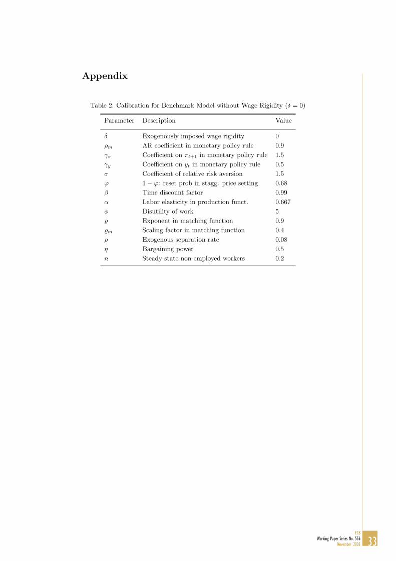
AIM.15 In order to analyze the dynamics of our model we calibrate the model choosing

parameter values that are generally used in the literature. The benchmark parameter

choices are displayed in Table 2.

In this section we analyze the model’s dynamics to a unit shock in monetary policy,

i.e. an increase in the nominal interest rate. We are particularly interested in how

monetary policy is propagated in the presence of a non-Walrasian labor market with

equilibrium unemployment and real wage rigidity. Towards that aim, we will compare

the outcome of the model under the two bargaining schemes introduced in the previous

sections, i.e. the efficient Nash bargaining and the right-to-manage bargaining. This

allows the analysis of the transmission process of monetary policy when labor markets

differ with respect to the bargaining regime as well as to the degree of wage rigidity.

The results regarding the impact of wage rigidity on the variables of interest crucially

depend on the prevailing bargaining regime.

3.1 Efficient Bargaining Setup

As a first step, we analyze the impact of wage rigidity when combined with an efficient

Nash bargaining setup. The corresponding impulse-response functions are displayed

in Figure 1. An adverse interest rate shock initially leads to a fall in private de-

mand. In order to adjust to private demand, intermediate good producers reduce

production, implying a fall in employment and working hours. A dampened demand

decreases expected profits and hence induces firms to post less vacancies. Vacancies

fall and unemployment increases accordingly. Since working hours must fall to meet

the reduced demand, firms pay lower wages to reduce worker’s labor supply.

The drop in consumption implies an increase in the current period’s marginal utility of

consumption. The marginal rate of substitution between leisure and consumption falls

accordingly. In Section 2.3.1 it was highlighted that the marginal rate of substitution

is an important determinant of firms’ marginal costs. As can be seen in Figure 1, a

15 See Anderson and Moore (1985) for details on the solution method.

21ECB


drop in the marginal rate of substitution is translated into a fall of marginal costs.

Additionally, inflation falls also since marginal costs subsequently affect inflation via

the New Keynesian Phillips curve.

The introduction of real wage rigidity in the efficient bargaining model increases the

adjustment via the employment margin. Under rigid wages, changes in demand con-

ditions have a stronger impact on the profits of the firm. If wages cannot decrease

sufficiently, firms are paying excessive wage compensation. This implies a negative

impact on firms’ profits, a reduced number of posted vacancies and an additional

reduction in employment. The path of hours, however, is not significantly affected,

which implies that inflation dynamics are not strongly influenced by the introduction

of wage rigidity.16

3.2 Right-to-Manage Bargaining Setup

As a second step, we analyze how the model dynamics change when workers and firms

bargain according to a right-to-manage (RTM) bargaining regime. We are particularly

interested in the responses of the variables when a wage rigidity is introduced into the

RTM model. For that reason we compare the response functions of a RTM model

without wage rigidity with a calibration using a high degree of wage stickiness. The

corresponding impulse-response functions are shown in Figure 2.

The initial reactions to a monetary policy shock without a wage norm are quite similar

to the responses in the efficient bargaining model. A noteworthy difference is that

wages react much stronger in the RTM model and labor flows are much less pronounced

than in the efficient bargaining version. The increased volatility of wages can be

explained by a steeper labor demand function in the right-to-manage setup.

The introduction of wage rigidity in the RTM model has an important implication for

the dynamics of inflation in the model, see Figure 2. Indeed, the introduction of wage

rigidities reduce the volatility and increase the persistence of wages. Accordingly, as

it is apparent from the figure, marginal costs and inflation also show a more persistent

response to a monetary policy shock. Therefore, we can show that for a reasonable

degree of wage rigidity the model improves significantly along the inflation persistence

margin.

16 This result is consistent with the findings of Krause and Lubik (2003).


In our model, rigid wages feed into marginal costs and hence have a direct impact

on inflation dynamics through the New Keynesian Phillips curve. The mechanism of

wage rigidities in the right-to-manage framework can be best seen in the linearized

version of the wage and inflation equation:17

wt = (1 − δ)(γ1mrst + γ2(vt − ut − ht − λt))

−(1 − δ)(γ3ht − ζ1χt + ζ2 E(χt+1)) + δwt−1 (32)

πt =(1 − βϕ)(1 − ϕ)

ϕ(wt − (α − 1)ht) + β E(πt+1) (33)

It is obvious from Equation (32) that the inclusion of wage rigidities smooth the path

of wages. Wages in turn determine firms’ marginal costs and thus directly feed into the

path of inflation, see Equation (33). Therefore, the wage rigidity smoothes marginal

costs and increases inflation persistence. Moreover, since in our model not only hours

but also employment adjusts to economic shocks, the fluctuations of hours can be

smaller than in a model without the employment margin. This implies that marginal

costs may be further smoothed by a less variable hours component. Therefore, the

modelling of flows in and out of employment in our model can have further implications

for the dynamics of marginal costs and hence inflation.

Table 1 displays the inflation and wage persistence from model simulations when

labor markets differ with respect to the bargaining regime as well as the degree of

wage rigidity. The four columns show the persistence in wages and inflation from the

model simulated series. Persistence is measured as the sum of the AR coefficients of

the respective lagged dependent variable from a univariate autoregressive process, see

Andrews and Chen (1994).18

The upper panel in Table 1 shows the model series persistence within a RTM bargain-

ing framework and the lower panel the efficient bargaining counterparts. It is apparent

17 Where χt = ηδw(1−χ)

ηχδw+(1−η)χhδw

t −

(1−η)χh

(ηχδw+(1−η)χh)δ

ft , variables with a hat denote the steady state

values and the parameters are given by the following relations: γ1 =1−η

(1+φ)+ η

α

1− ηα

, γ2 =(ηκ)

wqλh

1− ηα

, γ3 =(ηκ)

wqλh+

(1−η)b

wh

1− ηα

, ζ1 =η(1−α)(1−η)α

+ κ

qwλh

1− ηα

and ζ2 = η

1−η(1 − s)

κ

qwλh

1− ηα

.18 The most common approach to determine a variable’s persistence is to estimate a univariate AR

equation of the following form:

wt = c+ ςwt−1 +

4∑

i=1

ψi∆wt−i + εt

where ς corresponds to the sum of the AR coefficients of the lagged dependent variables. See e.g.Gadzinski and Orlandi (2003) for further evidence and alternative measures on inflation persistencein the euro area.

23ECB


Table 1: Estimated Persistence ς in Wages and Inflation

Bargaining Persistence Model Model Model Model.

Regime ς in δ = 0 δ = 0.90 δ = 0.95 δ = 0.97

Right to ManageWages 0.36 0.81 0.88 0.92

Inflation 0.38 0.71 0.77 0.78

Efficient BargainingWages 0.52 0.92 0.95 0.97

Inflation 0.17 0.18 0.19 0.16

Notes: δ is the coefficient of lagged wages in the wage equation.

from the table that the greater the exogenously imposed wage rigidity, the higher is

inflation persistence in the RTM model. For wage norms consistent with aggregate

wage data (e.g. an AR coefficient of 0.9) the RTM model generates substantial infla-

tion persistence compared to model variants with no wage norm. In contrast, inflation

persistence under the efficient bargaining framework is not affected significantly when

the degree of wage rigidity increases. In the efficient bargaining model there is no

direct channel from wages to firms’ marginal costs. Obviously, this prevents wages

from affecting inflation in a significant way.

To sum up, the introduction of RTM bargaining with real wage rigidities has important

implications for the transmission of monetary policy in the traditional New Keynesian

model. A non-clearing labor market together with wage rigidities help to explain a

more persistent response of inflation to a shock in interest rates.

4 The Impact of Labor Market Fundamentals

European labor markets are governed by labor market institutions such as collec-

tive wage bargaining, employment protection legislation and unemployment insurance.

These institutions may be seen to influence the bargaining power of workers which in

turn affect the wage determination process. In this section we look at the responses

of unemployment and inflation to a monetary policy shock under different degrees of

labor market rigidity in the RTM model with wage rigidity.19 The wage equation in

the right-to-manage model in Section 2.3.2 contains several variables characterizing

the state of the labor market such as the bargaining power of workers, the job de-

19 The notion of the interaction between shocks and institutions was forwarded by e.g. Blanchard andWolfers (2000) to statistically explain the evolution of European unemployment.


struction rate or the level of the reservation wage. Since we established a link between

the wage outcome and inflation dynamics, the question arises how the determinants

of the wage itself affect inflation dynamics.20

4.1 Bargaining Power of Workers

Collective wage bargaining is an important institutional feature that determines wages

of workers. For example, despite a relatively low union density, union coverage is fairly

high in most of Continental European countries, see e.g. Nickell, Nunziata, Ochel, and

Quintini (2003). Generally, higher bargaining power of workers in the form of higher

union membership and coverage is associated with an upward pressure on wages and

hence higher unemployment.21

We start with analyzing inflation and unemployment dynamics with different degrees

of workers’ bargaining power represented by the parameter, η, see Figure 3.22 If

bargaining power is high the negotiated wage increases since workers can command

higher wages for a given disutility of work. Thus, expected profits of firms decline and

cause the number of vacant jobs to fall. This in turn results in higher unemployment.

In line with the empirical evidence provided by e.g. Blanchard and Wolfers (2000), the

interaction of a monetary policy shock and high bargaining power leads to an increase

in unemployment in our model.

Higher bargaining power of workers induces inflation to respond more to a contrac-

tionary monetary policy shock, see Figure 3. When wages increase with higher bar-

gaining power, marginal costs rise as well and feed into increased movements of in-

flation. A change in bargaining power affects both the magnitude of the response in

unemployment and inflation and the persistence of the respective variables. Notice,

however, that an increase in bargaining power does not only feeds into larger upward

wage movements in the case of a positive demand shock, but due to the symmetry

of the model, also to larger wage declines when the shock is negative. Therefore,

20 Note that there have been a set of theoretical studies on the impact of labor market institutionssuch as hiring subsidies and unemployment benefits on labor market dynamics, see e.g. Yashiv(2004).

21 Yet, in practise this effect can be offset if wage setting in the economy is coordinated, see e.g.Nickell and Layard (1999).

22 The baseline parameter choice for bargaining power is η = 0.4 which is a conservative assumptionon rents accruing to the workers. Much empirical work has of course been devoted to estimatingbargaining power within a wage equation framework. For example Abowd and Lemieux (1993)estimated a workers’ share of rents of about 30% in Canada.

25ECB


higher wage movements translate also into larger movements in marginal costs and

thus larger responses in inflation.

4.2 Employment Protection

European labor markets are characterized by lower job turnover rates than their U.S.

counterpart, see e.g. Burda and Wyplosz (1994).23 This is conventionally interpreted

as stemming from higher employment protection and firing costs in Europe. On the

one hand, employment protection leads firms to be more cautious in filling vacancies

and on the other hand reduces involuntary separations. Lower job flows in our model

correspond to a lower job destruction rate. For that reason we model employment

protection simply through its effect on aggregate job flows. This neglects, however,

the direct effect of employment protection on the bargaining position of workers and

hence the impact on wages.

Figure 4 displays the responses of unemployment and inflation to a monetary policy

shock when we vary the rate of exogenous job destruction. In a regime with lower

job turnover, i.e. lower job destruction rates, unemployment reacts less to an adverse

interest rate shock since aggregate labor flows are lower.24 A lower job destruction

rate reduces aggregate job creation and elevates the volatility in real wages.25 Larger

adjustments on the wage margin dampen aggregate wage persistence. The response

of inflation to a monetary policy shock appears to be more pronounced and less per-

sistent. This in turn means that in the case of high aggregate labor flows, wage

adjustments tend to be small and thus translate into smaller and more persistent

movements of the inflation rate.26

The analysis has shown that any ”institutional” parameter that raises the volatility

in wages, increases also the response of inflation and tends to reduce its persistence.

On the other hand, anything that spurs the volatility in labor flows dampens the

adjustments of wages and, therefore, tends to increase the persistence in inflation.

23 A prominent exception is, however, the comparison of the U.S. and the Portuguese labor flows asdocumented in Blanchard and Portugal (2001).

24 Note that the empirical evidence of a relationship between employment protection and unemploy-ment is rather mixed, see e.g. Nickell and Layard (1999).

25 Notice that the effect on wages would be potentially larger if we had a direct channel of employmentprotection on the bargained wage outcome in our model.

26 In a similar vein, an increase in the natural rate of unemployment surges equilibrium job flows.Less adjustment takes place on the wage margin and, therefore, raises wage and hence inflationpersistence.


This, however, is partly due to the simplistic modelling of labor market institutions in

this model. Employment protection as well as bargaining power are usually associated

with exerting an upward pressure on wages with downward rigidity at the same time.

Since in our model wages react symmetrically, higher bargaining power results in

stronger wage increases in the case of a positive shock and in larger reductions in the

case of a negative shock, respectively. A better account of labor market institutions

and their implications for unemployment and inflation dynamics in this model, is a

task to be taken up in further research.

5 Conclusions

We include a labor market with wage rigidities as well as matching frictions into

the New Keynesian model. In particular, we follow the approach by Trigari (2003)

assuming that workers and firms bargain over wages according to a right-to-manage

bargaining model. We extend the Trigari setting by incorporating wage rigidity into

the right-to-manage bargaining framework which has important implications for the

joint dynamics of unemployment and inflation in our New Keynesian DSGE model.

The model sheds light on the question whether the specific form of wage bargaining

and the degree of wage rigidity affects the transmission process of monetary policy

determining inflation dynamics.

The traditional New Keynesian dynamic stochastic general equilibrium model of busi-

ness cycle fluctuations generally fails to account for the degree of inflation persistence

observed in actual data. Employing a right-to-manage bargaining framework, wages

feed directly into firm’s marginal cost and hence into inflation dynamics via the New

Keynesian Phillips curve. Introducing a wage rigidity in form of a Hall type wage

norm, we can show that more rigid wages translate into more persistent movements

of aggregate inflation. In contrast, the channel from wages to inflation is missing un-

der the assumption of an efficient bargaining model and, therefore, fails to generate

inflation persistence.

Our calibration also shows that unemployment and inflation dynamics do not only

depend on rigid wages but also on the parameters that determine employment protec-

tion, bargaining power of workers and the natural rate of unemployment. Generally,

”institutional” parameters that raise the volatility in wages, increase also the response

27ECB


of inflation and tend to reduce its persistence. On the other hand, anything that spurs

the volatility in labor flows, dampens the adjustments of wages and, therefore, tends

to increase the persistence in inflation.

The model reveals that the labor market has important implications for the trans-

mission process of monetary policy. The inclusion of a labor market into the New

Keynesian model introduces another channel along which real and nominal rigidities

can be incorporated into the model. The ”labor market channel” significantly affects

the dynamics of employment and inflation. In particular, real wage rigidity appears

to play a key role in shaping marginal cost dynamics and, consequently persistent

movement in inflation rates. Our model suggests that the central bank may benefit

from closely monitoring the labor market. From the developments in real labor flows

as well as real wage movements the central bank can infer on the dynamics and par-

ticularly, on the degree of persistence of the inflation rate. Therefore, differences in

labor market regimes may help to explain inflation dynamics across countries.

The theoretical results in our paper depend on the specific parameter choice in the

model’s calibration. In a companion paper, Christoffel, Kuster, and Linzert (2005),

the parameters of the model are estimated to make a quantitative assessment of the

model. In particular, we analyze the role of labor labor market rigidities for the

transmission of monetary policy. The estimated model allows us to make explicit

statements on the importance of wage rigidities for inflation dynamics. Moreover, we

shed light on the relevance of labor market shocks for business cycle dynamics and

monetary policy in particular.


References

Abowd, J., and T. Lemieux (1993): “The Effect of Product Market Competition on

Collective Bargaining Agreements: The Case of Foreign Competition in Canada,”

Quarterly Journal of Economics, 108, 983–1004.

Anderson, G., and G. Moore (1985): “A Linear Algebraic Procedure for Solving

Linear Perfect Foresight Models,” Economics Letters, 17, 247–52.

Andolfatto, D. (1996): “Business Cycles and Labor-Market Search,” American

Economic Review, 86(1), 112–132.

Andrews, D., and W. Chen (1994): “Approximately Median-Unbiased Estimation

of Autoregressive Models,” Journal of Business and Economics Statistics, 12, 187–

204.

Blanchard, O. J., and J. Gali (2005): “Real Wage Rigidities and the New Key-

nesian Model,” mimeo.

Blanchard, O. J., and P. Portugal (2001): “What Hides Behind an Unemploy-

ment Rate: Comparing Portuguese and US Unemployment,” American Economic

Review, 91(1), 187–207.

Blanchard, O. J., and J. Wolfers (2000): “The Role of Shocks and Institutions

in the Rise of European Unemployment: The Aggregate Evidence,” The Economic

Journal, 111, 1–33.

Boeri, T., and M. C. Burda (2003): “Preferences for Rigid versus Individualized

Wage Setting in Search Economies with Firing Frictions,” mimeo.

Burda, M., and C. Wyplosz (1994): “Gross Worker and Job Flows in Europe,”

European Economic Review, 38, 1287–1315.

Calvo, G. (1989): “Staggered Prices in a Utility Maximising Framework,” Journal

of Monetary Economics, 12, 383–398.

Christiano, L. J., M. Eichenbaum, and C. L. Evans (2005): “Nominal Rigidi-

ties and the Dynamic Effects of a Shock to Monetary Policy,” Journal of Political

Economy, 113(1), 1–45.

29ECB


Christoffel, K., K. Kuster, and T. Linzert (2005): “The Impact of Labor

Markets on the Transmission of Monetary Policy in an Estimated DSGE Model,”

mimeo.

Danthine, J.-P., and A. Kurmann (2004): “Fair Wages in a New Keynesian Model

of the Business Cycle,” Review of Economic Dynamics, 7, 107–142.

Edge, R. M., T. Laubach, and J. C. Williams (2003): “The Response of Wages

and Prices to Technology Shocks,” FRBSF Working Paper.

Erceg, C., J. D. W. Henderson, and A. T. Levin (2000): “Optimal Monetary

Policy with Staggered Wage and Price Contracts,” Journal of Monetary Economics,

46, 281–313.

Fuhrer, J. C., and G. Moore (1995): “Inflation Persistence,” The Quarterly Jour-

nal of Economics, February 1995, 127–159.

Gadzinski, G., and F. Orlandi (2003): “Inflation Persistence for the EU Countries

the EURO Area and the US,” mimeo, European Central Bank.

Gali, J., and M. Gertler (1999): “Inflation Dynamics: A Structural Econometric

Analysis,” Journal of Monetary Economics, 44, 195–222.

Gali, J., M. Gertler, and D. Lopez-Salido (2001): “European Inflation Dynam-

ics,” European Economic Review, 45, 1237–1270.

Hall, R. E. (2003): “Wage Determination and Employment Fluctuations,” Working

Paper 9967, NBER.

(2004): “The Labor Market is the Key to Understanding the Business Cycle,”

mimeo.

(2005): “Employment Fluctuations with Equilibrium Wage Stickiness,”

American Economic Review, 95(1), 50–65.

Krause, M. U., and T. A. Lubik (2003): “The (Ir)relevance of Real Wage Rigidity

in the New Keynesian Model with Search Frictions,” mimeo.

MacDonald, I., and R. M. Solow (1981): “Wage Bargaining and Employment,”

American Economic Review, 71, 896–908.


Merz, M. (1995): “Search in the Labor Market and the Real Business Cycle,” Journal

of Monetary Economics, 36(2), 269–300.

Mortensen, D., and C. Pissarides (1994): “Job Creation and Job Destruction in

the Theory of Unemployment,” Review of Economic Studies, 61, 397–415.

(1999): “Job Reallocation, Employment Fluctuations, and Unemployment

Differences,” in Handbook of Macroeconomics, ed. by J. Taylor, and M. Woodford,

pp. 1171–1228. Elsevier Science.

Nickell, S. J., and M. Andrews (1983): “Unions, Real Wage and Employment in

Britain 1951-79,” Oxford Economic Papers, 35, suppl., 183–206.

Nickell, S. J., and R. Layard (1999): “Labour Market Institutions and Economic

Performance,” in Handbook of Labor Economics, ed. by O. Ashenfelter, and D. Card.

North Holland.

Nickell, S. J., L. Nunziata, W. Ochel, and G. Quintini (2003): “The Beveridge

Curve, Unemployment and Wages in the OECD from the 1960s to the 1990s,” in

Knowledge, Information and Expectations in Modern Macroeconomics: In Honor

of Edmund S. Phelps, ed. by P. Aghion, R. Frydman, J. Stiglitz, and M. Woodford.

Princeton University Press.

Pissarides, C. A. (2000): Equilibrium Unemployment. MIT Press, second edn.

Rotemberg, J. J., and M. Woodford (1998): “An Optimization-Based Economet-

ric Framework for the Evaluation of Monetary Policy: Expanded Version,” NBER:

Technical Working Paper, 223.

Shimer, R. (2005): “The Cyclical Behavior of Equilibrium Unemployment, Vacancies

and Wages: Evidence and Theory,” American Economic Review, 95(1), 25–49.

Trigari, A. (2003): “Labor Market Search, Wage Bargaining and Inflation Dynam-

ics,” mimeo.

Uhlig, H. (2004): “Macroeconomics and Asset Markets: Some Mutual Implications,”

mimeo, Humboldt University Berlin.

Walsh, C. (2003): “Labor Market Search and Monetary Shocks,” in Elements of

Dynamic Macroeconomics, ed. by J. Altug, J. Chadha, and C. Nolan. Cambridge

University Press.

31ECB


Yashiv, E. (2004): “Macroeconomic Policy Lessons of Labor Market Frictions,” Eu-

ropean Economic Review, 48, 259–284.


Appendix

Table 2: Calibration for Benchmark Model without Wage Rigidity (δ = 0)

Parameter Description Value

δ Exogenously imposed wage rigidity 0

ρm AR coefficient in monetary policy rule 0.9

γπ Coefficient on πt+1 in monetary policy rule 1.5

γy Coefficient on yt in monetary policy rule 0.5

σ Coefficient of relative risk aversion 1.5

ϕ 1 − ϕ: reset prob in stagg. price setting 0.68

β Time discount factor 0.99

α Labor elasticity in production funct. 0.667

φ Disutility of work 5

Exponent in matching function 0.9

m Scaling factor in matching function 0.4

ρ Exogenous separation rate 0.08

η Bargaining power 0.5

n Steady-state non-employed workers 0.2

33ECB


Figure 1: Impulse-Response Functions of a Monetary Policy Shock from Calibrated Model inan Efficient Bargaining Regime

0 2 4 6 8 10 12 14 16 18 20−0.35

−0.3

−0.25

−0.2

−0.15

−0.1

−0.05

0

mcoeff

(a) Response of Marginal Cost

0 2 4 6 8 10 12 14 16 18 20−0.09

−0.08

−0.07

−0.06

−0.05

−0.04

−0.03

−0.02

−0.01

0

wageff

(b) Response of Real Wages

0 2 4 6 8 10 12 14 16 18 20−0.2

−0.15

−0.1

−0.05

0

0.05

vaceff

(c) Response of Vacancies

0 2 4 6 8 10 12 14 16 18 20−2

0

2

4

6

8

10

12

14

16x 10

−3

uneeff

(d) Response of Unemployment

0 2 4 6 8 10 12 14 16 18 20−0.06

−0.05

−0.04

−0.03

−0.02

−0.01

0

0.01

houeff

(e) Response of Hours of Work

0 2 4 6 8 10 12 14 16 18 20−0.07

−0.06

−0.05

−0.04

−0.03

−0.02

−0.01

0

piceff

(f) Response of Inflation

Notes: The dashed line corresponds to the impulse-responses of the efficient bargaining withoutexogenously imposed wage rigidity, i.e. δ = 0, see Equation (23). The solid line displays theimpulse-response function of the efficient bargaining model with wage rigidity of δ = 0.9. Noticethat this is not an implausible value as it corresponds to an estimated AR(1) coefficient for anunivariate real wage equation for U.S. and German data.


Figure 2: Impulse-Response Functions of a Monetary Policy Shock from Calibrated Model ina Right-to-Manage Bargaining Regime

0 2 4 6 8 10 12 14 16 18 20−0.35

−0.3

−0.25

−0.2

−0.15

−0.1

−0.05

0

0.05

mcortm

(a) Response of Marginal Cost

0 2 4 6 8 10 12 14 16 18 20−0.3

−0.25

−0.2

−0.15

−0.1

−0.05

0

0.05

wagrtm

(b) Response of Real Wages

0 2 4 6 8 10 12 14 16 18 20−0.08

−0.07

−0.06

−0.05

−0.04

−0.03

−0.02

−0.01

0

0.01

vacrtm

(c) Response of Vacancies

0 2 4 6 8 10 12 14 16 18 20−2

0

2

4

6

8

10x 10

−3

unertm

(d) Response of Unemployment

0 2 4 6 8 10 12 14 16 18 20−0.06

−0.05

−0.04

−0.03

−0.02

−0.01

0

0.01

hourtm

(e) Response of Hours of Work

0 2 4 6 8 10 12 14 16 18 20−0.07

−0.06

−0.05

−0.04

−0.03

−0.02

−0.01

0

0.01

picrtm

(f) Response of Inflation

Notes: The dashed line corresponds to the impulse-responses of the right-to-manage modelwithout exogenously imposed wage rigidity, i.e. δ = 0, see Equation (23). The solid line displaysthe impulse-response function of the right to manage model with wage rigidity of δ = 0.9. Noticethat this is not an implausible value as it corresponds to an estimated AR(1) coefficient for anunivariate real wage equation for U.S. and German data.

35ECB


Figure 3: Impulse-Response Functions of a Monetary Policy Shock from Calibrated Modelwith Decreased Workers’ Bargaining Power

0 2 4 6 8 10 12 14 16 18 20−0.04

−0.035

−0.03

−0.025

−0.02

−0.015

−0.01

−0.005

0

0.005

(a) Inflation

0 2 4 6 8 10 12 14 16 18 20−0.5

0

0.5

1

1.5

2

2.5

3

3.5x 10

−3

(b) Unemployment

Notes: The dashed line corresponds to the impulse-responses of the right-to-manage model withwage rigidity of δ = 0.9. The solid line displays the impulse-response function of the model witha decrease from 0.5 to 0.03 in worker’s bargaining power.


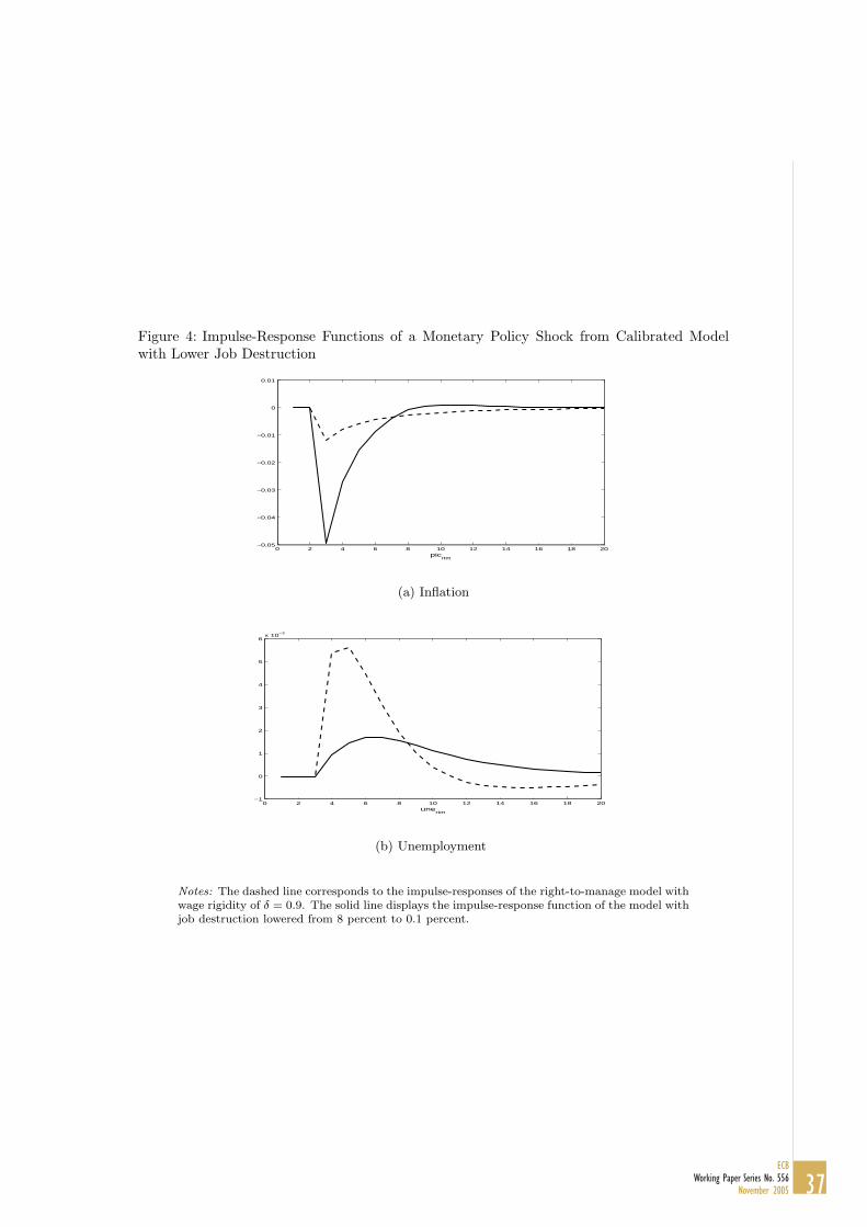
Figure 4: Impulse-Response Functions of a Monetary Policy Shock from Calibrated Modelwith Lower Job Destruction

0 2 4 6 8 10 12 14 16 18 20−0.05

−0.04

−0.03

−0.02

−0.01

0

0.01

picrtm

(a) Inflation

0 2 4 6 8 10 12 14 16 18 20−1

0

1

2

3

4

5

6x 10

−3

unertm

(b) Unemployment

Notes: The dashed line corresponds to the impulse-responses of the right-to-manage model withwage rigidity of δ = 0.9. The solid line displays the impulse-response function of the model withjob destruction lowered from 8 percent to 0.1 percent.

37ECB



European Central Bank working paper series

For a complete list of Working Papers published by the ECB, please visit the ECB’s website(http://www.ecb.int)

509 “Productivity shocks, budget deficits and the current account” by M. Bussière, M. Fratzscherand G. J. Müller, August 2005.

510 “Factor analysis in a New-Keynesian model” by A. Beyer, R. E. A. Farmer, J. Henryand M. Marcellino, August 2005.

511 “Time or state dependent price setting rules? Evidence from Portuguese micro data”by D. A. Dias, C. R. Marques and J. M. C. Santos Silva, August 2005.

512 “Counterfeiting and inflation” by C. Monnet, August 2005.

513 “Does government spending crowd in private consumption? Theory and empirical evidence forthe euro area” by G. Coenen and R. Straub, August 2005.

514 “Gains from international monetary policy coordination: does it pay to be different?”by Z. Liu and E. Pappa, August 2005.

515 “An international analysis of earnings, stock prices and bond yields”by A. Durré and P. Giot, August 2005.

516 “The European Monetary Union as a commitment device for new EU Member States”by F. Ravenna, August 2005.

517 “Credit ratings and the standardised approach to credit risk in Basel II” by P. Van Roy,August 2005.

518 “Term structure and the sluggishness of retail bank interest rates in euro area countries”by G. de Bondt, B. Mojon and N. Valla, September 2005.

519 “Non-Keynesian effects of fiscal contraction in new Member States” by A. Rzońca andP. Ciz· kowicz, September 2005.

520 “Delegated portfolio management: a survey of the theoretical literature” by L. Stracca,September 2005.

521 “Inflation persistence in structural macroeconomic models (RG10)” by R.-P. Berben,R. Mestre, T. Mitrakos, J. Morgan and N. G. Zonzilos, September 2005.

522 “Price setting behaviour in Spain: evidence from micro PPI data” by L. J. Álvarez, P. Burrieland I. Hernando, September 2005.

523 “How frequently do consumer prices change in Austria? Evidence from micro CPI data”by J. Baumgartner, E. Glatzer, F. Rumler and A. Stiglbauer, September 2005.

524 “Price setting in the euro area: some stylized facts from individual consumer price data”by E. Dhyne, L. J. Álvarez, H. Le Bihan, G. Veronese, D. Dias, J. Hoffmann, N. Jonker,P. Lünnemann, F. Rumler and J. Vilmunen, September 2005.

39ECB


525 “Distilling co-movements from persistent macro and financial series” by K. Abadir andG. Talmain, September 2005.

526 “On some fiscal effects on mortgage debt growth in the EU” by G. Wolswijk, September 2005.

527 “Banking system stability: a cross-Atlantic perspective” by P. Hartmann, S. Straetmans andC. de Vries, September 2005.

528 “How successful are exchange rate communication and interventions? Evidence from time-seriesand event-study approaches” by M. Fratzscher, September 2005.

529 “Explaining exchange rate dynamics: the uncovered equity return parity condition”by L. Cappiello and R. A. De Santis, September 2005.

530 “Cross-dynamics of volatility term structures implied by foreign exchange options”by E. Krylova, J. Nikkinen and S. Vähämaa, September 2005.

531 “Market power, innovative activity and exchange rate pass-through in the euro area”by S. N. Brissimis and T. S. Kosma, October 2005.

532 “Intra- and extra-euro area import demand for manufactures” by R. Anderton, B. H. Baltagi,F. Skudelny and N. Sousa, October 2005.

533 “Discretionary policy, multiple equilibria, and monetary instruments” by A. Schabert,October 2005.

534 “Time-dependent or state-dependent price setting? Micro-evidence from German metal-workingindustries” by H. Stahl, October 2005.

535 “The pricing behaviour of firms in the euro area: new survey evidence” by S. Fabiani, M. Druant,I. Hernando, C. Kwapil, B. Landau, C. Loupias, F. Martins, T. Y. Mathä, R. Sabbatini, H. Stahl andA. C. J. Stokman, October 2005.

536 “Heterogeneity in consumer price stickiness: a microeconometric investigation” by D. Fougère,H. Le Bihan and P. Sevestre, October 2005.

537 “Global inflation” by M. Ciccarelli and B. Mojon, October 2005.

538 “The price setting behaviour of Spanish firms: evidence from survey data” by L. J. Álvarez andI. Hernando, October 2005.

539 “Inflation persistence and monetary policy design: an overview” by A. T. Levin and R. Moessner,November 2005.

540 “Optimal discretionary policy and uncertainty about inflation persistence” by R. Moessner,November 2005.

541 “Consumer price behaviour in Luxembourg: evidence from micro CPI data” by P. Lünnemannand T. Y. Mathä, November 2005.

542 “Liquidity and real equilibrium interest rates: a framework of analysis” by L. Stracca,November 2005.


543 “Lending booms in the new EU Member States: will euro adoption matter?”by M. Brzoza-Brzezina, November 2005.

544 “Forecasting the yield curve in a data-rich environment: a no-arbitrage factor-augmentedVAR approach” by E. Mönch, November 2005.

545 “Trade integration of Central and Eastern European countries: lessons from a gravity model”by M. Bussière, J. Fidrmuc and B. Schnatz, November 2005.

546 “The natural real interest rate and the output gap in the euro area: a joint estimation”by J. Garnier and B.-R. Wilhelmsen, November 2005.

547 “Bank finance versus bond finance: what explains the differences between US and Europe?”by F. de Fiore and H. Uhlig, November 2005.

548 “The link between interest rates and exchange rates: do contractionary depreciations make adifference?” by M. Sánchez, November 2005.

549 “Eigenvalue filtering in VAR models with application to the Czech business cycle”by J. Beneš and D. Vávra, November 2005.

550 “Underwriter competition and gross spreads in the eurobond market” by M. G. Kollo,November 2005.

551 “Technological diversification” by M. Koren and S. Tenreyro, November 2005.

552 “European Union enlargement and equity markets in accession countries”by T. Dvorak and R. Podpiera, November 2005.

553 “Global bond portfolios and EMU” by P. R. Lane, November 2005.

554 “Equilibrium and inefficiency in fixed rate tenders” by C. Ewerhart, N. Cassola and N. Valla,November 2005.

555 “Near-rational exuberance” by J. Bullard, G. W. Evans and S. Honkapohja, November 2005.

556 “The role of real wage rigidity and labor market frictions for unemployment and inflationdynamics” by K. Christoffel and T. Linzert, November 2005.

WORKING PAPER SERIES - ecb.europa.eu · THE ROLE OF REAL WAGE RIGIDITY AND LABOR ... and Andrew...

Documents

Transcript of WORKING PAPER SERIES - ecb.europa.eu · THE ROLE OF REAL WAGE RIGIDITY AND LABOR ... and Andrew...