WORKING PAPER SERIES - ecb.europa.eu · For instance, the model by Dees et al. (2007), which...

WORK ING PAPER SER IE SNO 855 / JANUARY 2008

ASSESSING THEFACTORS BEHINDOIL PRICE CHANGES

by Stéphane Dées,Audrey Gasteuil,Robert K. Kaufmannand Michael Mann

WORKING PAPER SER IESNO 855 / J ANUARY 2008

ASSESSING THE FACTORSBEHIND OIL PRICE CHANGES 1

by Stéphane Dées 2,Audrey Gasteuil 3,

Robert K. Kaufmann 4

and Michael Mann 5

This paper can be downloaded without charge fromhttp : //www.ecb.europa.eu or from the Social Science Research Network

electronic library at http : //ssrn.com/abstract id=1080247.

1 The views expressed in this paper are those of the authors and do not necessarily refl ect the position of the European Central Bank or the Eurosystem. We are grateful to colleagues of the European Central Bank and the Eurosystemas well as an anonymous referee

for helpful comments.2 European Central Bank, Kaiserstrasse 29, D-60311 Frankfurt am Main, Germany; e-mail: [email protected]

3 Currently at Société Générale, 52 Place de l’Ellipse, 92972 Paris La Défense Cedex, France; e-mail: [email protected]. The paper was written while the author visited

the European Central Bank as an intern.4 Center for Energy & Environmental Studies, Department of Geography and Environment,

Boston University, Boston, MA 02215, United States; e-mail: [email protected] Department of Geography and Environment, Boston University, Boston, MA 02215,

United States; e-mail: [email protected]

In 2008 all ECB publications

feature a motif taken from the €10 banknote.

© European Central Bank, 2008

Address Kaiserstrasse 29 60311 Frankfurt am Main, Germany

Postal address Postfach 16 03 19 60066 Frankfurt am Main, Germany

Telephone +49 69 1344 0

Website http://www.ecb.europa.eu

Fax +49 69 1344 6000

All rights reserved.

Any reproduction, publication and reprint in the form of a different publication, whether printed or produced electronically, in whole or in part, is permitted only with the explicit written authorisation of the ECB or the author(s).

The views expressed in this paper do not necessarily refl ect those of the European Central Bank.

The statement of purpose for the ECB Working Paper Series is available from the ECB website, http://www.ecb.europa.eu/pub/scientific/wps/date/html/index.en.html

ISSN 1561-0810 (print) ISSN 1725-2806 (online)

3ECB

Working Paper Series No 855January 2008

Abstract 4

Non-technical summary 5

1 Introduction 7

2 Methodology 9

3 Results 15

4 Discussion 17

Conclusion 27

Literature cited 28

Figure caption 30

Figures and tables 31

European Central Bank Working Paper Series 36

CONTENTS

4ECBWorking Paper Series No 855January 2008

ABSTRACT

The rapid rise in the price of crude oil between 2004 and the summer of 2006 are the subject

of debate. This paper investigates the factors that might have contributed to the oil price

increase in addition to demand and supply for crude oil, by expanding a model for crude oil

prices to include refinery utilization rates, a non-linear effect of OPEC capacity utilization,

and conditions in futures markets as explanatory variables. Together, these factors allow the

model to perform well relative to forecasts implied by the far month contracts on the New

York Mercantile Exchange and are able to account for much of the $26 rise in crude oil prices

between 2004 and 2006.

Keywords: Oil prices, Refinery industry, OPEC

JEL codes: C53, Q41.

5ECB


Non-technical summary

The rapid rise in the price of crude oil between 2004 and the summer of 2006 are the subject

of debate. This paper investigates the factors that might have contributed to the oil price increase

in addition to demand and supply for crude oil.

The first additional factor is related to the changes in the so-called downstream sector;

especially the refining sector. The number of refineries in the United States has not increased

since 1981, and in the spring of 2007, a significant fraction of refining capacity was closed due

to unscheduled maintenance. Under these conditions, a lack of spare refining capacity is seen as

one cause for the on-going rise in the price of motor gasoline and crude oil.

Other factors proposed to explain the sharp rise in oil prices include the lack of sufficient

spare production capacity and a non-linear relationship between oil prices and supply. The

existence of non-linearities in the relationship between oil prices and the quantity delivered to the

market might affect the determination of oil prices. Although a linear relationship could be a

reasonable approximation under normal circumstances, extreme events may shift the market

equilibrium between supply and demand towards different types of market functioning in which

prices are much more sensitive to shocks than under normal conditions. Non-linearities may be

caused by lags associated with building additional extraction and refining capacity. Given these

constraints, oil prices would be more sensitive to supply as production approaches capacity.

Finally, expectations of shortages in the long-run may also influence oil prices. The

conditions on the futures markets (whether the market is contango - the price of crude oil for four

month contracts is greater than the price for near month contracts - or in backwardation - the

price of crude oil for four month contracts is less than the price for the near month contract-)

might therefore affect the stock behaviors and, in turn, the oil price setting.

In this paper, we estimate a model for crude oil prices that includes refinery utilization rates,

a non-linear effect of OPEC capacity utilization, and conditions in futures markets (New York


Mercantile Exchange) as explanatory variables. Results indicate that the refining sector plays an

important role in the recent price increase, but not in the way described by most analysts. The

relationship is negative such that higher refinery utilization rates reduce crude oil prices. This

effect is associated with shifts in the production of heavy and light grades of crude oil and price

spreads between them. Non-linear relationships between OPEC spare capacity and oil prices as

well as conditions on the futures markets also account for changes in real oil prices. Together,

these factors allow the model to perform well relative to forecasts implied by the far month

contracts on the New York Mercantile Exchange and are able to account for much of the $26 rise

in crude oil prices between 2004 and 2006.

7ECB


I Introduction

Causes for the rapid rise in the price of crude oil between 2004 and the summer of 2006 are

the subject of debate. Some of the debate focuses on changes in the so-called downstream

sector; especially the refining sector. The number of refineries in the United States has not

increased since 1981 (Annual Energy Review, 2006), and in the spring of 2007, a significant

fraction of refining capacity was closed due to unscheduled maintenance (New York Times,

2007). Under these conditions, a lack of spare refining capacity is seen as one cause for the on-

going rise in the price of motor gasoline and crude oil. Other factors proposed to explain the

sharp rise in oil prices include the lack of sufficient spare production capacity and a non-linear

relationship between oil prices and supply. Finally, expectations of shortages in the long-run may

also influence oil prices.

Arguments that such factors might be important determinants of oil prices are consistent with

the performance of models that exclude their effect. For instance, the model by Dees et al.

(2007), which specifies crude oil prices as a function of OPEC capacity, OECD crude oil stocks,

OPEC quotas and cheating by OPEC on those quotas, performs well in-sample, but consistently

under-predict real oil prices since 2004 (Figure 1).

While causal relationships in the US oil supply chain indicate that the price of crude oil is

exogenous and that downstream factors such as refinery utilization rates have no effect on the

price of crude oil (Kaufmann et al., in review), statistical models used to estimate the causal

relationships do not contain many of the factors that are known to affect crude oil prices, such as

capacity utilization, production quotas, and production levels (Kaufmann et al., 2004; Wirl and

Kujundzic, 2005). Moreover, the existence of non-linearities in the relationship between oil

prices and the quantity delivered to the market might affect the determination of oil prices.

Although a linear relationship could be a reasonable approximation under normal circumstances,

extreme events may shift the market equilibrium between supply and demand towards different


types of market functioning in which prices are much more sensitive to shocks than under

normal conditions. Non-linearities may be caused by lags associated with building additional

extraction and refining capacity (Kaufmann and Cleveland, 2001; Kaufmann, in review). Given

these constraints, oil prices would be more sensitive to supply as production approaches

capacity. Finally, the conditions on the futures markets (whether the market is in contango - the

price of crude oil for four month contracts are greater than the price for near month contracts - or

in backwardation - the price of crude oil for four month contracts is less than the price for near

month contracts-) might affect the stock behaviors and, in turn, the oil price setting.

In this paper, we estimate a model for crude oil prices that includes refinery utilization rates,

a non-linear effect of OPEC capacity utilization, and conditions in futures markets (New York

Mercantile Exchange) as explanatory variables. Results indicate that the refining sector plays an

important role in the recent price increase, but not in the way described by most analysts. The

relationship is negative such that higher refinery utilization rates reduce crude oil prices. This

effect is associated with shifts in the production of heavy and light grades of crude oil and price

spreads between them. Non-linear relationships between OPEC spare capacity and oil prices as

well as conditions on the futures markets also account for changes in real oil prices. Together,

these factors allow the revised model to perform well relative to forecasts implied by the far

month contracts on the New York Mercantile Exchange and are able to account for much of the

$26 rise in crude oil prices between 2004 and 2006.

These results and the methods used to obtain them are described in five sections. Section II

describes the data and econometric techniques used to estimate a cointegrating relationship for

crude oil prices. Results are described in section III. Section IV discusses the effect of refinery

utilization rates on crude oil prices, the importance of non-linearities in supply conditions, and

the role of futures market conditions. It also presents the ability of this econometric equation to

forecast oil prices. Section V concludes.

9ECB


II Methodology

To explore the effect of downstream conditions on crude oil prices, we update the quarterly

data set used to estimate the price equation described by Kaufmann et al. (2004) and expand it to

include other market conditions, such as US refinery utilization rates and conditions in the New

York Mercantile Exchange. Because there are a large number of I(1) explanatory variables, the

cointegrating relationship for crude oil prices is estimated using the dynamic ordinary least

squares (DOLS) developed by Stock and Watson (1993). Short run dynamics are estimated

using an error correction model.

Data

The quarterly data set (1986Q1-2000Q4) used by Kaufmann et al. (2004) to evaluate the

effect of OPEC on crude oil prices includes observations on the average F.O.B price for all crude

oil imported by the US, OPEC capacity utilization, OPEC quotas, OECD oil demand, and OECD

stocks of crude oil. We use the average FOB price for crude oil imported by the US as the

dependent variable because it represents the price paid for physical barrels obtained from a

variety of sources. As such, it is relatively unaffected by conditions unique to a single market.

For example, the price of West Texas Intermediate (WTI) is influenced by local conditions, such

as stocks of crude oil in Cushing Oklahoma and conditions in refineries that depend heavily on

WTI. These data are updated with observations through 2006Q4, the most recent quarter for

which a complete set of data is available.

To evaluate the effect of conditions in the refining sector on crude oil prices, we collect data

on US refinery utilization rates, which vary between zero and one. Monthly observations are

available from the Energy Information Administration. Ideally, we would prefer global data, but

only US data are available; nonetheless, US refinery capacity utilization is a satisfactory proxy

as US refinery capacity represents about 20 percent of world capacity in 2006. Indeed, as there is


one global market, even for refined petroleum products, it is unlikely that utilization rates in one

part of the world will decouple dramatically from other parts. So long as one can ship refined

petroleum products, it is, for instance, unlikely that US refinery utilization rates will increase

significantly while European rates will decline significantly1. Finally, if the greatest shortage of

refining capacity does occur in the US, then US refinery utilization rates are the relevant measure

because they would reflect conditions at the margin, which by definition, determine prices.

This notion is based on results that indicate the price of crude oil produced in geographical

disparate parts of the world cointegrate (e.g. Bachmeier and Griffin, 2006). If refinery utilization

rates affect crude oil prices, cointegration among crude prices implies that refinery utilization

rates in different parts of the globe share the same stochastic trend. If refinery utilization rates do

not share the same stochastic trend, the different stochastic trends in refinery utilization rates

would prevent cointegration among different types of crudes. If refinery utilization rates do not

affect crude prices, statistical results will fail to reject the null hypothesis of no relationship

between refinery utilization rates and crude oil prices, regardless of which refinery utilization

rate is used in the statistical model.

Refinery utilization rates affect crude oil prices based on the ability of refineries to convert

crude oil to final products. Crude oil is available in different qualities: sour and sweet, heavy

and light. Refineries are designed to operate most efficiently using specific crudes such that the

values of crude rises and falls based on the availability of specific types of crude relative to

existing refining capacity. Although currently much of the world’s refining capacity is set up to

use light sweet crudes, heavy sour crudes represent much of the unused production capacity in

OPEC. However, rapidly rising demand for refined oil products and growing supplies of crude

1 For example, immediately after hurricane Katrina that hit the Gulf of Mexico in September 2005, there was a very large increase in US imports of finished motor gasoline during September and October 2005 relative to the same months during 2004. Presumable, non-US refiners increased their utilization rates to generate this extra gasoline.

11ECB


oil have squeezed spare refining capacity. Bottlenecks have also arisen in the downstream oil

industry through a lack of de-sulphurisation capacity and limited conversion capacity, reflecting

limited investment in the industry in the recent years. The marginal barrel of crude oil that

refiners are able to process is of a light and sweet quality. However, the marginal supply of crude

oil is of a heavy and sour quality. There is thus a quality mismatch between the marginal barrel

of oil supplied and the marginal barrel of oil that refiners are able to process. This mismatch may

affect crude oil markets.

To evaluate the effect of conditions in the New York Mercantile Exchange, we compile

observations on the near month contract and the four-month contract for West Texas

Intermediate (Cushing--dollars per barrel). To generate quarterly observations, we average

values for days on which contracts are traded. We use these data to calculate the spread

between the near month and four month contract. This difference is used to measure whether the

market is in contango or in backwardation. Finally, we compile quarterly observations for the US

GDP price deflator in order to compute oil prices in real terms.

Model Explanation

To represent the effect of refinery utilization rates, nonlinearities, and conditions in the New

York Mercantile Exchange on crude oil prices, we estimate the following equation:

Pricet = + 1Dayst + 2Caputilt + 3Caputil2t + 4 Caputil3

t+ 5 Refinet

+ 6 (NYMEX4t- NYMEX1 )t + t (1)

in which Price is the real average F.O.B. price for US crude oil imports (2000 US$). Days is

days of forward consumption of OECD crude oil stocks, which is calculated by dividing OECD

stocks of crude oil by OECD demand for crude oil. Caputil is capacity utilization by OPEC,

which is calculated by dividing OPEC production by OPEC capacity, multiplying this quotient

by OPEC’s share of global oil production, and dividing this product by the rate at which OPEC


cheats on its quota (dividing the difference between OPEC production and OPEC quota by world

oil demand)2. Refine is the US refinery utilization rate. NYMEX4 is the fourth month contract for

WTI and NYMEX1 is the near month contract for WTI.

We expect the regression coefficient associated with Days to be negative — an increase in

stocks reduces real oil price by reducing reliance on current production and thereby lowering the

risk premium that is associated with a supply disruption.

We also expect a negative relationship between refinery utilization rates and crude oil prices.

This effect can be understood two ways. Increasing rates of refinery utilization forces refiners to

buy crudes that are less well suited to refineries. This reduces their yield and reduces the value of

products they produce. Similarly, as refineries reach capacity, the demand for crude oil drops,

which also reduces prices.

The cubic specification chosen for Caputil allows for two turning points (or inflection

points). We expect 2 and 4 to be positive and 3 to be negative. Under these conditions, prices

increase exponentially up to the first turning point and increase exponentially after the second

turning point. Between these turning points there is a normal operating range in which changes in

capacity utilization have small impacts on prices. This relationship is based on the assumption

that producers prefer to lift oil within a normal operating range. At levels well above this range,

high utilization rates can interfere with field maintenance that is needed to ensure the long-run

productivity of the well. Similarly, operators are reluctant to pump at very low utilization rate

because fixed costs of production are very much greater than operating costs — so long as prices

remain above operating costs operators will desire to operate their wells to pay off their fixed

costs. Desire to operate within this range coupled with inelastic price elasticities of demand

2 We modify Caputil by cheating because cheating could increase capacity utilization by OPEC but reduce oil prices by increasing supply relative to the quota that balances world oil demand and non-OPEC production. To account for this effect, Caputil is divided by cheat. This division allows increased rates of cheating to reduce oil prices even as cheating causes capacity utilization to rise-

13ECB


imply that prices must change significantly to move refinery utilization rates back towards the

normal operating range. As capacity utilization rises beyond normal operating conditions and

supplies become tight, inelastic demand implies that large prices increases are needed to bring

utilization rates back to the normal range. On the downside, inelastic price elasticities imply very

large price reductions are needed to increase demand (or make it economical to decommission

capacity) to move capacity utilization back towards the normal operating range. Similar

arguments can be made for a non-linear effect of refinery utilization, but the squared and cubic

terms of refinery utilization are not statistically different from zero.

Finally, we expect 6 to be positive as contango is expected to have a positive effect on

prices because the higher price for future deliveries provides an incentive to build and hold

stocks, which bolsters demand.

Econometric Methodology

As indicated by previous analyses, time series for the real price of crude oil and its

determinants probably contain a stochastic trend. We evaluate the time series properties of

variables in equation (1) using the Augmented Dickey Fuller statistic (Dickey and Fuller, 1979)

and a test statistic for quarterly data (Hylleberg et al., 1990). Results in Table 1 indicate that

these variables contain an annual root. The ADF statistic fails to reject the null hypothesis of a

unit root for all variables (Table 1 – Panel “Univariate tests”). This result is generally confirmed

by the 1 statistic, which fails to reject the null hypothesis of no annual root for variables other

than Caputil and Days. None of the variables contain seasonal unit roots, as indicated by results

that reject 2 = 0 and a joint test. F 3 4 0.

The presence of I(1) trends invalidates the blind application of ordinary least squares (OLS)

because the diagnostic statistics generated by OLS will indicate a meaningful relationship among

unrelated I(1) variables more often than implied by random chance (Granger and Newbold,


1974). Such relations are termed spurious regressions. To avoid confusion that is associated

with spurious regressions, the relationship among variables in equation (1) is evaluated by

determining whether they cointegrate. Following a well established method to determine

whether two (or more) variables cointegrate (Engle and Granger, 1987), equation (1) is estimated

by OLS. In such a case the regression error ( ) would be analyzed for a stochastic trend using the

ADF and HEGY statistic. If these test statistics fail to reject the null hypothesis, the

nonstationary residual indicates that the regression is spurious. If the regression error is

stationary, the variables cointegrate. In this case, equation (1) can be interpreted as a

cointegrating relationship for real oil prices.

However, even if the variables cointegrate, the OLS estimate of the cointegrating vector will

contain a small sample bias and the limiting distribution will be non-normal with a non-zero

mean (Stock, 1987). In this paper, to avoid confusion associated with this bias, the cointegrating

relationship among non-stationary variables in equation (1) is estimated using dynamic ordinary

least squares (DOLS) (Stock and Watson, 1993). DOLS generates asymptotically efficient

estimates of the regression coefficients for variables that cointegrate, it is computationally

simple, and it performs well relative to other asymptotically efficient estimators (Stock and

Watson, 1993). Coefficients estimated by DOLS represent the long run relationship among

variables. DOLS does not estimate the short-run dynamics -- it is not necessary for

asymptotically efficient estimation of the cointegrating vector. Lags and leads used to estimate

the DOLS version of equation (1) are chosen using the Schwarz Information criterion (Schwarz,

1978). The large number of variables in equation (1) would make it difficult to identify

cointegrating relationships using the full information maximum likelihood (FIML) estimator of a

vector error correction model developed by Johansen (1988) and Johansen and Juselius (1990). If

there is a cointegrating relationship between oil prices and the right-hand side variables in

15ECB


equation (1), then we need to examine the short run relationship among variables. To do so, we

use OLS to estimate an error correction model (ECM), which is given by equation (2):

t

s

iiti

s

iititi

s

iiti

s

iiti

s

iiti

s

iiti

s

iititt

WarQQQ

PriceNYMEXNYMEXRefine

CaputilCaputilCaputilDayskPrice

4332211

17

16

15

1

33

1

22

11

111

14 (2)

in which is the first difference operator, Q1, Q2, and Q3, are dummy variables for the first,

second, and third quarters respectively, War is a dummy variable for the first Persian Gulf War

(1990Q3-1990Q4), and is the residual from the cointegrating relationship estimated in

equation (1). The number of lags (s) for the right-hand side variables in equation (2) is chosen

using the Akaike information criterion (Akaike, 1973).

The statistical significance of in equation (2) evaluates the hypothesis that prices are

affected by disequilibrium between observed real oil prices and the right hand side variables in

equation (1), which represents the long-run value. A negative value for indicates that

disequilibrium between crude oil prices and its determinants moves price toward the equilibrium

value implied by the cointegrating relationship. Under these conditions, the right hand side

variables in equation (1) are said to 'Granger cause' real oil prices.

III Results

Regression results for equation (1) indicate that the variables constitute a cointegrating

relationship that can be interpreted as an equation for the long-run determinants of real oil prices.

The ADF statistic for the OLS regression error rejects the null hypothesis of a unit root, which

indicates that there are no unit roots at an annual frequency (Table 1 – Panel “DOLS Regression

residuals”). This conclusion is reinforced by the value of 1, which also rejects the null


hypothesis of a unit root at an annual frequency. Nor does the residual contain unit roots at sub-

annual frequencies, as indicated by results that reject 2 = 0 and a joint test F 3 4 0.

The elements of the cointegrating vector have signs that are generally consistent with

previous results (Table 2). The effect of Days is negative. An increase in stocks reduces

reliance on current production, which tends to lower the risk premium that is associated with a

supply disruption. Capacity utilization by OPEC producers has a positive effect on prices. But

unlike previous efforts, the weighted effect of capacity utilization is represented in a nonlinear

fashion. The signs of the regression coefficients are consistent with a priori expectations that

prices drop rapidly at low levels of capacity utilization and rise rapidly at high levels of capacity

utilization.

As expected, the coefficient associated with the difference between the four-month and near

month contract for WTI on the New York Mercantile Exchange is positive, indicating that

contango has a positive effect on prices. Finally, the coefficient associated with refinery

utilization rates is negative. As explained in the next section, this negative effect is associated

with changes in the types of crude oil produced and price spreads between crude oils of different

densities.

Regression results for the error correction model (equation (2)) indicate that the cointegrating

relationship given by equation (1) can be interpreted as an equation for the long-term

determinants of price. The error correction term ( ) in equation (2) is negative. This value

indicates that disequilibrium among oil prices and the right-hand side variables from equation (1)

move oil price towards the long-run equilibrium value that is implied by the right hand side

variables. As such, OECD stocks, OPEC capacity utilization rates, refinery utilization rates, and

conditions in the New York Mercantile Exchange “Granger cause” real oil prices. Furthermore,

this effect is very rapid. The point estimate for indicates that 68 percent of the difference

17ECB


between the equilibrium and observed price for crude oil is eliminated within one quarter (Table

2). But the standard error around the point estimate implies that we cannot reject the null

hypothesis = -1 ( t= 1.77, p > 0.083), which would indicate that prices adjust completely.

IV Discussion

The Effect of Refinery Utilization on Crude Oil Prices

The sign associated with refinery utilization ( 5) in equation (1) is negative—higher refinery

utilization rates depress crude oil prices. This negative effect could be seen as counterintuitive as

the lack of new refining capacity is mostly seen as partially responsible for higher prices. Killian

(2007) however finds similar results with the reduced-form model of oil prices (crude and

gasoline prices). Moreover, the negative effect of refinery utilization rates is consistent with the

effect of refinery utilization rates on the composition of crude oils produced and price spreads

between crude oils of varying densities.

The effect of refinery utilization rates on the price of crude oil is associated with changes in

the quality of crude oils produced. The quality of a crude oil is determined in large part by its

density and sulfur content. The density of crude oil is measured by an API gravity index, which

measures the density of crude oil relative to water. An API value of greater than 10o indicates

that crude floats on water, with larger values indicating a reduction in density (i.e. lighter crude).

In general, light grades of crude oils are of higher quality because they generate greater yields of

more valuable light products (e.g. motor gasoline). Crude oils with a high sulfur content (so-

called sour crudes) are of lower quality because they increase refinery maintenance costs due to

enhanced corrosion associated with the sulfur. Based of these differences, the price for a barrel

of light sweet crude generally is greater than the price for heavy and sour grades of crude oils.


For example, the price Arabian medium during the fourth quarter of 2006 was $54.38 per

barrel—a barrel of Arabian Heavy cost $52.26. The $2.11 difference is termed the price spread.

At any point in time, producers from around the globe lift an array of crude oils. Because of

their higher price, light, sweet crudes tend to be produced first. For producers, these crudes

generate greater revenues. For refiners, light sweet crudes increase revenues and reduce costs.

As refinery utilization rates rise, producers increase the production of heavy sour crudes. For

example, Saudi Arabia increased its production of crude oil from 7.52 million barrels per day

(MBD) in 1999 to 9.15 MBD in 2005. Of this 1.63 MBD increase, 1.58 MBD came from

medium grades of crude oil—the production of light grades of crude oil increased only 0.053

MBD (Eni Spa, 2006). Because of the price spread among crude oils, the change in the

composition of crude oil reduced the average price of crude oil produced by Saudi Arabia. Note

that the dependent variable in equation (1) is an average of crude oil purchased by the US. So,

an increase in refinery utilization rates reduces the average price of crude oil by changing the

composition of crude oil imports in favor of heavy and sour grades of crude oil.

Refinery utilization rates also may affect prices by changing the spread between the price of

heavy and light grades of crude oil. As refinery utilization moves towards capacity, increased

demand is satisfied by expanding runs of heavy and sour crudes. But prices may drop as the

quality declines and demand weakens. As utilization rates reach 100 percent, demand drops to

zero. These effects suggest that increases in refinery utilization rates may lower prices of

medium and heavy crude oils more than they raise the price of light crude oils. This too would

lower the price of crude oil as refiner utilization rates rise.

To test the hypothesis that increased refinery utilization rates reduce the price of heavy

grades of crude oil relative to lighter grades, we investigate the effect of refinery utilization rates

on the price spread between grades of crude oils by estimating equations (3) – (6):

19ECB


Heavy 1 1Medium 1Util 1t (3)Medium 2 2Heavy 2Util 2t (4)

Heavy 1 1 1t 1 1i Mediumt i

i 1

s

1i Utilt i

i 1

s

1t (5)

Medium 2 2 2t 1 2i Heavyt i

i 1

s

2i Utilt i

i 1

s

1t (6)

in which Heavy is the nominal price of Arabian Heavy (API index = 27o), Medium is the nominal

price of Arabian Medium (31o), and Util is the US refinery utilization rate. The estimation

sample includes weekly observations between January 3, 1997 and May 18, 2007 that are

obtained from the Energy Information Administration. The sample period represents the longest

periods of nearly continuous data. Because the time series for price and utilization rates contain

stochastic trends, equations (3) - (6) are estimated using the same general procedure used to

estimate equations (1) and (2).

Equations (3) and (4) test the hypothesis that refinery utilization rates do not affect the spread

between heavy and medium grades of crude oil produced by Saudi Arabia. This null hypothesis

is tested by evaluating i = 0 in equations (3) and (4). Rejecting the null hypothesis 1= 0 and/or

2 = 0 would indicate that refinery utilization rates affect the price spread. To ensure that DOLS

can estimate these coefficients reliably, ADF statistics calculated from the OLS residual suggest

that equation (3) can be viewed as a cointegrating relationship for Arabian Heavy and equation

(4) can be viewed as a cointegrating relationship for Arabian Medium (Table 3). The DOLS

estimate of 1 in equation (3) indicates that increases in refinery utilization rates depress the price

of Arabian Heavy relative to Arabian Medium—the DOLS estimate for 2 in equation (4)

indicates that increases in refinery utilization rates increase the price of Arabian Medium relative

to Arabian Heavy, but this effect is measurable only at the ten percent level (Table 3). These

results are consistent with the hypothesis that refinery utilization rates affect the price spread

between crude oils.


The estimate for 1 in equation (5) suggests (p < .06) that disequilibrium in the cointegrating

relationship estimated from equation (3) moves the price of Arabian Medium towards its

equilibrium value. Conversely, the estimate for 2 in equation (6) indicates that disequilibrium

in equation (4) has no effect on the price of Arabian Medium. This suggests that the effect of

refinery utilization rates on price spreads is manifest largely by reductions in the price of heavy

grades of crude oil—this simple model does not provide evidence that higher refinery utilization

rates raise the price of lighter crude oils. As such, these results are consistent with the hypothesis

that higher refinery utilization rates reduce the price of heavier crude oils.

To assess further the effects of the refinery utilization on the oil market, we simulate a

decrease in the refinery utilization rate by 5% in the model by Dees et al (2007) supplemented

with the new oil price equations (1) and (2). Figure 2 shows that a 5 percentage point reduction

in refinery utilization rate would increase crude oil prices by around 20%, which depressed

world demand by about 0.5%. Higher oil prices increase non-OPEC production (about 1%),

which combined with lower demand, reduce OPEC production by about 2.5% after 2 years (2%

in the long-run).

Non-linearities in supply conditions and dynamics in crude oil prices

To check the importance of non-linearities in the oil price behaviors, we use several tests to

evaluate the inclusion of nonlinear terms in equation (1). First, values for 3 and 4 that are

significantly different from zero give preliminary support for a nonlinear relationship. Second,

we test whether non-linear combinations of the estimated values help explain the dependent

variable (Ramsey, 1974). This procedure is based on the notion that if non-linear combinations

of the explanatory variables have any power in explaining the dependent variable, then the linear

model is misspecified. Test statistics indicate that a linear version of equation (1) is indeed

misspecified, which confirms the role of nonlinear terms of Caputil in determining real oil prices

21ECB


(Table 4). Finally, we evaluate the role of nonlinearities using F-tests for omitted and/or

redundant variables. The former checks whether additional variables (here the non-linear terms)

explain a significant portion of the variation in the dependent variable; the latter tests whether a

subset of variables (here the non-linear terms) all have zero coefficients and may be deleted from

the equation. Both tests confirm the validity of the non-linear specification of the oil price

equation (Table 5).

To assess the impact of non-linearities on the oil prices, we introduce equations (1) and (2)

in the model by Dees et al. (2007) to assess a demand shock (rise by 1% in world real GDP). We

simulate two scenarios: the first assumes that OPEC operates at 96% of its capacity (i.e. broadly

the highest level of OPEC capacity utilization that was reached in 2005Q3); the second case

assumes that OPEC operates at 87% of its capacity (Figure 3). The price increase is more rapid at

higher rates of utilization. As the model equilibrates, the long-term response is the same; non-

linearities affect the dynamics of convergence. This simulation illustrates that high rates of

OPEC capacity utilization amplified the price effects of demand growth after 2004.

Contango, Backwardation & Speculation

It is a bit surprising that equations (1) and (2) credit the change from backwardation to

contango with a significant effect on real crude oil prices. This effect may represent a change in

expectations for long-run prices. Both backwardation and contango are stable market conditions

that are maintained by self-reinforcing positive feedback loops and significant shifts between

these two states can be triggered by an exogenous shift in expectations.

The market has been in a general period of backwardation between 1998 and 2005. During

this period, prices were relatively low and demand was relatively weak. Under these conditions,

OPEC tried to maintain prices by keeping the market tight. By pumping just enough oil to cover

demand, there was no oil “left over” to build stocks and the lack of stocks supported higher

prices in the near month. Prices were lower farther in the future because there was plenty of


spare capacity. Backwardation is maintained via the incentive to hold stocks and speculative

behaviors. So long as the market is in backwardation, there is no incentive to build stocks

because future deliveries can be purchased at a lower price and do not carry the economic costs

of physical storage. Backwardation can be broken only if OPEC produces quantities of oil well

beyond its quota, raises its production quotas beyond immediate market demand, or if demand

starts to grow faster than trend growth.

Since 2005, the market has entered a period of contango, in which prices on contracts for

future deliveries are higher than prices on contracts for current deliveries. Under these

conditions, stocks of crude oil build if the price difference between far-month and the near-

month contract is greater than the economic cost of physically holding oil. Financial gains are

available to those who can store oil via purchase of prompt-month contracts and sell contracts

dated further in the future. The stock build reinforces contango by lowering near month prices.

Contango can be broken if the market perceives a long-term slow-down in demand growth or a

long-term increase in production growth.

Given the positive feedback loops that maintain backwardation and contango, significant shifts

between these two stable states probably need to be driven largely by exogenous events. To

date, analysts have not isolated an exogenous event that changed the market from backwardation

to contango. Failing this, the switch may be associated with a change in long-run perceptions for

oil prices. Specifically, the lack of significant additions to OPEC capacity, continued discussion

about a peak in global oil supply, and strong growth in oil demand despite higher prices, may

have raised the far-end of the price curve in a way that moved the market from backwardation to

contango.

Forecasting performance and factors explaining the recent rise in oil prices

Evaluating the effect of refinery utilization rates, non-linearities, and conditions in the futures

market on crude oil prices is motivated by efforts to explain the recent rise in crude oil prices

23ECB


(2004-2006). To assess the degree to which this price rise can be explained by equations (1) and

(2), we use them to generate a one-step ahead out-of-sample forecast. The forecast is compared

to those implied by the futures market and a random walk. To facilitate comparisons with

alternative forecasts, equations (1) and (2) are re-estimated using the price for the near month

contract of WTI on the NYMEX as the dependent variable. By doing so, the one step ahead out-

of sample forecast for the near month contract can be compared directly to that implied by the

futures market, which is the price for the four month contract (there is no equivalent set of

potential forecasting variables for the average FOB price used as the dependent variable in the

previous section). The forecast implied by a random walk is the current price (level) for the near

month contract applied to the next quarter.

Equations (1) and (2) (hereafter termed oil price model) are used to generate a recursively

expanding, one-step ahead forecast from the second quarter of 1999 through the first quarter of

2007. Visual comparison indicates that equations (1) and (2) are able to generate an accurate one

step ahead out of sample forecast (Figure 1). The single notable exception is the forecast for the

third quarter of 2003, when the model under predicts the observed value. The third quarter

coincides with the start of the US occupation of Iraq, and the model may not be able to capture

its effect on global oil prices. The model’s ability to reconstruct the recent price rise is not solely

due to the one-step ahead nature of the forecast. If we start the simulation in the first quarter of

1999 and do not update the observed prices for crude oil, the model still captures much of the

recent rise in oil prices (Figure 1).

To compare the oil price model’s forecast to the futures market and a random walk, the

accuracy of the forecasts are assessed using the following loss function:

dt Ptˆ PEt

2Pt

ˆ PAt2

(7)


in which Pt is the observed price for crude oil at time t, ˆ PEt the one-step ahead out-of-sample

price forecast by the econometric model and ˆ PAt is the price forecast by the alternative model,

either the futures market or a random walk.

Values of dt are used to calculate the sign test (S2a) test statistic as follows:

S2a

I dt 0.5Nt 1

N

0.25N(8)

1 0( )

0t

t

if dI d

otherwise

in which N is the number of observations (32) (Lehmann, 1975). The S2a statistic tests the null

hypothesis that the price forecasts generated by the two models are equally accurate and is

asymptotically standard normal under the null. A negative value for the S2a statistic that exceeds

the p = .05 threshold (-1.96) would indicate that the one step ahead out-of-sample forecast

generated by the econometric model is closer to the observed value of price than the alternative

forecast more often than expected by random chance. Under these conditions, we would

conclude that the econometric model generates a more accurate price forecast than the futures

market or a random walk.

Results indicate that the econometric model performs relatively well. The one-step-ahead

forecast generated by the econometric model is statistically indistinguishable from the forecast

implied by far month contracts on the NYMEX. The forecast generated by the econometric

model is closer to the observed value for sixteen of the thirty-two out-of sample observations,

hence the zero value (p=1.0) for the S2a statistic. On the other hand, there is some indication that

the one step ahead forecast based on the notion that oil prices are a random walk is more accurate

than the forecast generated by the oil price model. The value of the sign test is 1.77, which

25ECB


indicates that that the random walk is closer to the observed value than expected by random

chance at the ten percent level (p < .086). The superior performance of a random walk is

consistent with previous studies that indicate the price forecasts implied by the futures contracts

perform poorly relative to random walks (Abosendra and Baghestani, 2004).

The oil price forecasts also can be compared using the econometric concept of

encompassing. For competing forecasts, a finding of encompassing means that relative to a first

forecast, a second forecast provides no further useful incremental information for prediction

(Newbold and Harvey, 2002). In other words, the second model contains no information not

already contained in the first model, which makes the second forecast inferentially redundant.

Our analysis of encompassing is based on the notion that the three models can be thought

of nested versions of the other. The econometric model includes the difference of the near and

four month contract on the NYMEX, and so forecasts based on the four month contract or a

random walk can be thought of as restricted versions of the econometric model.

To test whether one model encompasses another, we use a test statistic (ENC-NEW)

developed by Clark and McCracken (2001). Their test statistic is given by:

ENC NEW P

P 1 ( ˆ 1,i2 ˆ 1,i ˆ 2,i )

i t 1

N

P 1 ( ˆ 2,i2 )

i t 1

N

in which P is the number of one step ahead forecasts (32), ˆ 1 is the error of one step ahead

forecast generated by the restricted model, ˆ 2 is the error of the one step ahead forecast

generated by the unrestricted model, t+1 is the date of the first out of sample forecast (1999Q2),

N is the date for the last out of sample forecast (2007Q1). The null hypothesis is that model 2

nests the restricted model 1 such that model 2 therefore contains k extra parameters. Rejecting


this null would indicate that the extra k parameters in model 2 are not redundant. This null

hypothesis is tested against a non-standard distribution whose critical value depends on the

number of extra parameters (k) and the ratio of out of sample observations to the number of in

sample observations, which is termed P (.64 for this analysis)

We fail to reject the null hypothesis (ENC-NEW = 2.69, k=5, p > .05) that the econometric

model contains five excess parameters (capacity utilization - together with its square and cubic

terms, refinery utilization, and stocks). This result is consistent with the results that the random

walk generates a more accurate out-of-sample forecast than the econometric model. On the other

hand, we reject (ENC-New = 7.7, p < .01) the null hypothesis that the four-month contract on

the NYMEX nests the econometric model, which implies that the five parameters in the

econometric model are not superfluous—they contain information not in the four-month

contract.

Given the oil price model’s ability to generate an accurate one step ahead out-of-sample

forecast, we use the econometric model to quantify the causes for the increase in the average

FOB oil price for US oil imports between 2004Q1 and 2006Q3. To isolate the effects of

individual variables, we simulate the model with historical observations for that variable and

hold all other right hand variables at their value in 2004Q1. The price change associated with

that variable is the difference between the simulated value for the third quarter 2006 and the

observed value for the first quarter 2004.

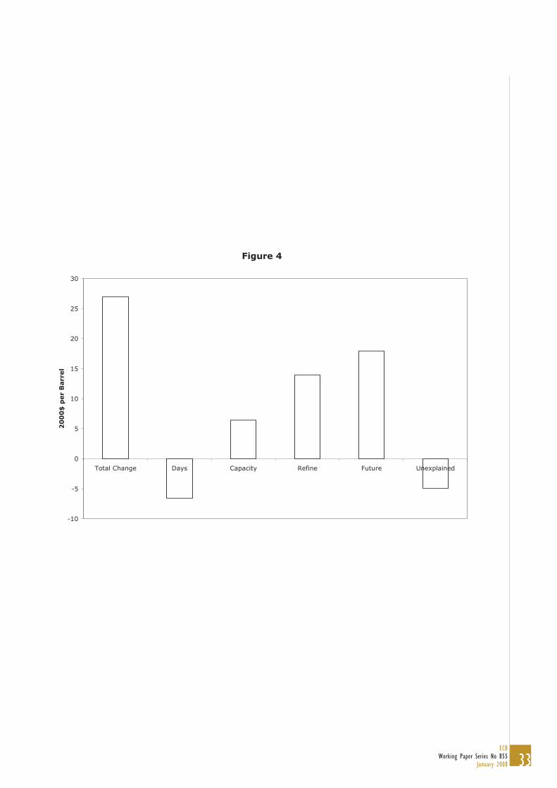
Results indicate that much of the $26.94 increase is associated with an increase in OPEC’s

capacity utilization, changes in refinery utilization rates, and changes in the futures market

(Figure 4). Specifically, the effects of the OPEC capacity utilization variable raised prices by

about $6.49 largely because of a steady decline in OPEC cheating—OPEC capacity rose from 94

percent in 2004Q2 to 96.3 percent in 2005Q3, but then dropped back to 94.7 percent in 2006Q2.

US refinery utilization rates dropped from 95.2 percent in 2004Q2 to 90.7 percent in 2006Q2 and

27ECB


this decline is associated with a $13.97 price rise. The difference between the near-month and

four month contract for WTI rose from –0.96 in 2004Q1 to $2.39 in 2006Q2, which raised oil

prices by about $17.93. Offsetting these increases, OECD stocks of crude oil rose from 81.7

days to 86.2 days and this reduced oil prices by $6.55. Together, these effects overstate the

observed price rise by $4.90.

Conclusion

The rapid rise in the price of crude oil between 2004 and the summer of 2006 has been

difficult to explain with the usual fundamentals related to the supply/demand balance. This paper

investigates additional factors that might have contributed to the oil price increase. Most of the

increase can be explained by concerns about future oil market conditions, materialized by the

shift of the futures market in contango, as well as changes in the refining sector, with a drop in

the refinery utilization rate. Factors related to crude oil supply continued to be important when

we account for non linear relationships between OPEC spare capacity and oil prices.

Interestingly, results of this analysis indicate that there is little evidence that increasing

refining capacity could lower crude oil prices. Of the variables identified by this paper to effect

prices, only stocks of crude oil could effectively participate to lower prices —each days of

forward consumption reduces real oil prices by about $2 in the long run. However, despite a

recent upturn, days of forward consumption have generally declined over the last twenty years,

from about 90-95 days of forward consumption to 78-82 days of forward consumption.

Interestingly, this reduction is not due to a reduction in stock levels, but to the fact that the

increase in storage capacity has been considerably slower than the increase in demand. This

implies that market conditions may not provide the economic incentives needed to expand

storage facilities with demand. Against this background, as long as demand remains robust, there

are very few reasons to expect oil prices to return to levels observed before 2004.


Literature cited

Abosendra, S. and H. Baghestani (2004), On the predictive accuracy of crude oil production

futures prices, Energy Policy, 32(12), 1389-1393.

Akaike, H. (1973), 2nd International Symposium on Information Theory, P.N. Petrov and F.

Csaki, Eds., Akadacemiai Kiadaco, 267-281.

Annual Energy Review (2006), Table 5.9, US Energy Information Agency, Washington, DC.

Bachmeier, L.J. and J.M. Griffin (2006), Testing for market integration crude oil, coal, and

natural gas, The Energy Journal 27(2), 55-71.

Clark, T. and M. McCracken (2001), Tests of equal forecast accuracy and encompassing for

nested models, Journal of Economertrics, 105, 85-110.

Dees, S. P. Karadeloglou, R. Kaufmann, and M. Sanchez (2007), Modelling the World Oil

Market, Assessment of a quarterly Econometric Model, Energy Policy, 35, 178-191.

Dickey, D. A. and W. A Fuller (1979), Distribution of the estimators for autoregressive time

series with a unit root. Journal of American Statistics Association, 74, 427-431.

Engle, R.E. and C.W.J., Granger (1987), Cointegration and error-correction: representation,

estimation, and testing, Econometrica, 55, 251-276

Granger, C. W. J. and P. Newbold (1974), Spurious regressions in econometrics, Journal of

Econometrics, 2, 111-120.

Hylleberg, S, R.F. Engle, L.W.J. Granger, and B.S. Yoo (1990), Seasonal integration and

cointegration, Journal of Econometrics, 44, 215-238.

Johansen, S. and K. Juselius (1990), Maximum likelihood estimation and inference on

cointegration with application to the demand for money, Oxford Bulletin of Economics and

Statistics, 52, 169-209.

Johansen, S. (1988), Statistical analysis of cointegration vectors, Journal of Economic Dynamics

and Control, 12, 231-254

29ECB


Kaufmann, R.K. (2007), US refining capacity: implications for environmental regulations and

the production of alternative fuels, CEES Working paper.

Kaufmann, R.K. and C.J. Cleveland (2001), Oil production in the lower 48 states; Economic,

geological, and institutional determinants, The Energy Journal, 22, 27-49.

Kaufmann, R.K, S. Dees, P. Karadeloglou, and M. Sanchez (2004), Does OPEC matter? an

econometric analysis of oil prices, The Energy Journal, 25(4), 67-90.

Kaufmann, R.K, S. Dees, and M. Mann (In review), Causal order in the US oil supply chain, The

Energy Journal.

Killian, L. (2007), The Economic Effects of Energy Price Shocks, Journal of Economic

Literature, forthcoming.

Lehmann, E.L. (1975), Nonparametrics, Statistical Methods Based on Ranks McGraw-Hill, San

Francisco.

Mackinnon, J.A. (1996), Numerical distribution functions for unit root and cointegration tests,

Journal Applied Econometrics,11, 601-618.

Newbold, P. and D.I. Harvey (2002), Forecast Combination and Encompassing, In: A

Companion to Economic Forecasting M. P. Clements and D.F. Hendry (eds.) Blackwell

Publishers, Malden, MA.

New York Times (2007), Record failures at oil refineries raise gas prices, July 22.

Ramsey, J.B. (1974), Classical model selection through specification error tests, in P. Zarembka

(ed), Frontiers in Econometrics new York, Academic Press.

Schwarz, G. (1978), Estimating the dimension of a model, Annals of Statistics, 6, 461-464.

Stock, J.H. (1987), Asymptotic properties of least squares estimators of co-integrating vectors,

Econometrica 55, 1035-1056.

Stock, J.H. and M.W. Watson (1993), A simple estimator of cointegrating vectors in higher order

integrated systems, Econometrica, 61, 783-820.


Wirl, F. and A. Kujundzic (2004), The impact of OPEC conference outcomes on world oil

prices 1984-2001, The Energy Journal, 25(1), 45-62.

Figure Caption

Figure 1 The observed value of the near month contract on the NYMEX (solid line). The

forecast for the average prices for US crude oil imports generated by a model that omits the

effects of refinery utilization, non-linearities, and market conditions in the NYMEX (dotted

line). The one-step ahead out of sample forecast generated by the econometric model

(equations (1) & (2)) is given by open circles (root mean square error = 4.07), the forecast

implied by the near month contract on the NYMEX is given by the open squares (root mean

square error = 3.54), a random walk, as given by the lagged value of the near month contract

on the NYMEX(mean square error = 3.08). Open diamonds represent the price simulated by

the econometric model with information about the exogenous variables only (root mean

square error = 6.87).

Figure 2 Impact of a 5 percent decrease in refinery utilization as measured by the percentage

changes from the baseline scenario.

Figure 3 Impact of a 1 percent increase in world real GDP on oil prices as measured by the

percentage change from the baseline scenario.

Figure 4 The change in real oil price between the first quarter of 2004 and the second quarter of

2006 explained by different individual variables in equations (1) and (2).

31ECB


Figure 1

0

10

20

30

40

50

60

70

1999-1 2000-1 2001-1 2002-1 2003-1 2004-1 2005-1 2006-1 2007-1

20

00

Do

llars

per

Barr

el


Figure 2

-3.0

-2.5

-2.0

-1.5

-1.0

-0.5

0.0

0.5

1.0

1.5

1 5 9 13 17 21 25 29 33 37 41 45 49 53 57 61 65 69 73 77 81 85

-60

-50

-40

-30

-20

-10

0

10

20

30

World demand Opec supply Non-Opec supply Crude oil price (rhs)

Figure 3

0

0.5

1

1.5

2

2.5

3

3.5

1 4 7 10 13 16 19 22 25 28 31 34 37 40 43 46 49 52 55 58 61 64 67 70 73 76 79 82

OPEC cap. util. at 96% OPEC cap. util. at 87%

33ECB


Figure 4

-10

-5

0

5

10

15

20

25

30

Total Change Days Capacity Refine Future Unexplained

20

00

$ p

er

Barr

el


Table 1 - HEGY statistics for annual and seasonal unit rootsADF F

Univariate tests Price -0.93 -0.57 -3.23** -4.97** -1.26 14.85** Days -2.31 -3.49+ -4.29** -6.94** 0.01 21.07** Caputil -2.07 -1.36 -2.58 -5.45** -4.21** 35.93** Refine -1.53 -5.51** -4.63** -5.10** -1.70+ 15.52** NYMEX1-NYMEX4 -2.44 -2.40 -2.69 -5.25** -3.07** 18.61** DOLS Regression residuals

quation (1) -4.81+ -3.89** -4.89** -6.32** -1.82* 23.85** ** Value exceeds p < .01, *p < .05, and + p < .10 Univariate HEGY tests include an intercept, time trend, and seasonal dummies. HEGY statistic calculated from the OLS regression residuals do not include an intercept, time trend, or seasonal dummies. Significance levels from Hylleburg et al., (1990). Univariate ADF test includes an intercept time trend, and seasonal dummies. ADF tests of cointegrating relation do not include a constant or intercept. Number of augmenting lags chosen using the Akaike information criterion (Akaike, 1973). Significance levels from Mackinnon (1996) using the number of observations. Asymptotic values have a higher significance level.

Table 2 - Estimates for Price Equation US FOB Price NYMEX Price Cointegrating Relation (Equation 1) Constant 382.80**

{23.27} 435.07** {19.94}

Days -2.06** {0.14}

-2.39** {0.12}

Caputil 2.46** {0.58}

2.37** {0.54}

Caputil2 -1.01E-01** {3.30E-02}

-9.31E-02** {3.00E-02}

Caputil3 7.84E-04** {2.96E-04}

7.17E-04** {1.25E-04}

Refine -2.09** {0.15}

-2.29** {0.13}

NYMEX1-NYMEX4 3.25** {0.40}

4.08** {0.36}

R2 0.91 0.94 Short run Dynamics (Equation 2) 3 Adjustment rate ( ) -0.68**

(0.18) -0.70** (0.19)

R2 0.61 0.60 {} standard error calculated using the Newey-West (1987) estimator ** Value exceeds p < .01, *p < .05, and + p < .10

3 We do not report the full set of results as too many parameters have been estimated. These results are available upon request.

35ECB


Table 3 - Regression results for spreads between the price of Arabian Heavy and Arabian Medium (equations (3) –(6))

Equations (3) & (5) Equations (4) & (6) Medium ( 1) 9.46E-01**

Heavy ( 2) 1.06** Util ( ) -3.26E-02* 3.25E-02+

-2.33E-01+ 3.00E-02 ADF# -3.21+ -3.24+ Length for lags and leads for the ADF test, the DOLS estimators, or the OLS estimator is chosen based on the statistical significance of lags and leads—missing values prevent the use of standard statistical criteria such as the Akaike or Schwarz criteria.

** Value exceeds p < .01, *p < .05, and + p < .10 # ADF statistic does not have a trend or a constant. Significance level calculated based on

functions in MacKinnon (1996) using the number of observations. Asymptotic values have a higher significance level.

Table 4 - Ramsey test for non-linearities in the oil price equation

Reset 1 15.04 (0.000) Reset 2 7.38 (0.001) The p-value associated with the statistic is in parenthesis. Note: The Ramsey RESET tests 1 and 2 use the fitted values squared, the fitted values squared and cubed as explanatory regressors respectively.

Table 5 - Tests for non-linearities in the oil price equation (Omitted and redundant variable test)

Omitted variables, F-stat 3.87 (0.027) Redundant variables, F-stat 11.99 (0.000) The p-value associated with the statistic is in parenthesis.


European Central Bank Working Paper Series

For a complete list of Working Papers published by the ECB, please visit the ECB’s website(http://www.ecb.europa.eu).

817 “Convergence and anchoring of yield curves in the euro area” by M. Ehrmann, M. Fratzscher, R. S. Gürkaynak and E. T. Swanson, October 2007.

818 “Is time ripe for price level path stability?” by V. Gaspar, F. Smets and D. Vestin, October 2007.

819 “Proximity and linkages among coalition participants: a new voting power measure applied to the International Monetary Fund” by J. Reynaud, C. Thimann and L. Gatarek, October 2007.

820 “What do we really know about fi scal sustainability in the EU? A panel data diagnostic” by A. Afonsoand C. Rault, October 2007.

821 “Social value of public information: testing the limits to transparency” by M. Ehrmann and M. Fratzscher, October 2007.

822 “Exchange rate pass-through to trade prices: the role of non-linearities and asymmetries” by M. Bussière, October 2007.

823 “Modelling Ireland’s exchange rates: from EMS to EMU” by D. Bond and M. J. Harrison and E. J. O’Brien, October 2007.

824 “Evolving U.S. monetary policy and the decline of infl ation predictability” by L. Benati and P. Surico,October 2007.

825 “What can probability forecasts tell us about infl ation risks?” by J. A. García and A. Manzanares, October 2007.

826 “Risk sharing, fi nance and institutions in international portfolios” by M. Fratzscher and J. Imbs, October 2007.

827 “How is real convergence driving nominal convergence in the new EU Member States?” by S. M. Lein-Rupprecht, M. A. León-Ledesma, and C. Nerlich, November 2007.

828 “Potential output growth in several industrialised countries: a comparison” by C. Cahn and A. Saint-Guilhem, November 2007.

829 “Modelling infl ation in China: a regional perspective” by A. Mehrotra, T. Peltonen and A. Santos Rivera, November 2007.

830 “The term structure of euro area break-even infl ation rates: the impact of seasonality” by J. Ejsing, J. A. García and T. Werner, November 2007.

831 “Hierarchical Markov normal mixture models with applications to fi nancial asset returns” by J. Gewekeand G. Amisano, November 2007.

832 “The yield curve and macroeconomic dynamics” by P. Hördahl, O. Tristani and D. Vestin, November 2007.

833 “Explaining and forecasting euro area exports: which competitiveness indicator performs best?” by M. Ca’ Zorzi and B. Schnatz, November 2007.

834 “International frictions and optimal monetary policy cooperation: analytical solutions” by M. Darracq Pariès, November 2007.

835 “US shocks and global exchange rate confi gurations” by M. Fratzscher, November 2007.

37ECB


836 “Reporting biases and survey results: evidence from European professional forecasters” by J. A. Garcíaand A. Manzanares, December 2007.

837 “Monetary policy and core infl ation” by M. Lenza, December 2007.

838 “Securitisation and the bank lending channel” by Y. Altunbas, L. Gambacorta and D. Marqués, December 2007.

839 “Are there oil currencies? The real exchange rate of oil exporting countries” by M. M. Habiband M. Manolova Kalamova, December 2007.

840 “Downward wage rigidity for different workers and fi rms: an evaluation for Belgium using the IWFP procedure” by P. Du Caju, C. Fuss and L. Wintr, December 2007.

841 “Should we take inside money seriously?” by L. Stracca, December 2007.

842 “Saving behaviour and global imbalances: the role of emerging market economies” by G. Ferrucci and C. Miralles, December 2007.

843 “Fiscal forecasting: lessons from the literature and challenges” by T. Leal, J. J. Pérez, M. Tujula and J.-P. Vidal, December 2007.

844 “Business cycle synchronization and insurance mechanisms in the EU” by A. Afonso and D. Furceri,December 2007.

845 “Run-prone banking and asset markets” by M. Hoerova, December 2007.

846 “Information combination and forecast (st)ability. Evidence from vintages of time-series data” by C. Altavillaand M. Ciccarelli, December 2007.

847 “Deeper, wider and more competitive? Monetary integration, Eastern enlargement and competitiveness in the European Union” by G. Ottaviano, D. Taglioni and F. di Mauro, December 2007.

848 “Economic growth and budgetary components: a panel assessment for the EU” by A. Afonso andJ. González Alegre, January 2008.

849 “Government size, composition, volatility and economic growth” by A. Afonso and D. Furceri, January 2008.

850 “Statistical tests and estimators of the rank of a matrix and their applications in econometric modelling”by G. Camba-Méndez and G. Kapetanios, January 2008.

851 “Investigating infl ation persistence across monetary regimes” by L. Benati, January 2008.

852 “Determinants of economic growth: will data tell?” by A. Ciccone and M. Jarocinski, January 2008.

853 “The cyclical behavior of equilibrium unemployment and vacancies revisited” by M. Hagedorn and I. Manovskii, January 2008.

854 “How do fi rms adjust their wage bill in Belgium? A decomposition along the intensive and extensive margins”by C. Fuss, January 2008.

855 “Assessing the factors behind oil price changes” by S. Dées, A. Gasteuil, R. K. Kaufmann and M. Mann,January 2008.

WORKING PAPER SERIES - ecb.europa.eu · For instance, the model by Dees et al. (2007), which...

Documents

Transcript of WORKING PAPER SERIES - ecb.europa.eu · For instance, the model by Dees et al. (2007), which...