Working paper research - | nbb.be · Working paper research n° 68 ... Member of the Board of...
71
Working paper research n° 68 May 2005 Noname – A new quarterly model for Belgium Philippe Jeanfils Koen Burggraeve
Transcript of Working paper research - | nbb.be · Working paper research n° 68 ... Member of the Board of...

Working paper research n° 68 May 2005
Noname – A new quarterly model for Belgium Philippe Jeanfi ls Koen Burggraeve

NBB WORKING PAPER No 68 – MAY 2005
NATIONAL BANK OF BELGIUM
WORKING PAPERS - RESEARCH SERIES
NONAME
A NEW QUARTERLY MODEL FOR BELGIUM_______________________________
Philippe Jeanfils (*)
Koen Burggraeve (**)
The views expressed in this paper are those of the authors and do not necessarily reflect
the views of the National Bank of Belgium.
We are especially grateful to Raf Wouters for his helpful comments on this paper. Any
remaining errors are of course our sole responsibility.
(*) NBB, Research Department, (e-mail: [email protected]).(**) NBB, Research Department, (e-mail: [email protected]).

NBB WORKING PAPER No 68 – MAY 2005
Editorial Director
Jan Smets, Member of the Board of Directors of the National Bank of Belgium
Statement of purpose:
The purpose of these working papers is to promote the circulation of research results (Research Series) and analyticalstudies (Documents Series) made within the National Bank of Belgium or presented by external economists in seminars,conferences and conventions organised by the Bank. The aim is therefore to provide a platform for discussion. The opinionsexpressed are strictly those of the authors and do not necessarily reflect the views of the National Bank of Belgium.
The Working Papers are available on the website of the Bank:http://www.nbb.be
Individual copies are also available on request to:NATIONAL BANK OF BELGIUMDocumentation Serviceboulevard de Berlaimont 14BE - 1000 Brussels
Imprint: Responsibility according to the Belgian law: Jean Hilgers, Member of the Board of Directors, National Bank of Belgium.Copyright © fotostockdirect - goodshoot
gettyimages - digitalvisiongettyimages - photodiscNational Bank of Belgium
Reproduction for educational and non-commercial purposes is permitted provided that the source is acknowledged.ISSN: 1375-680X

NBB WORKING PAPER No 68 – MAY 2005
Abstract
This paper gives an overview of the present version of the quarterly model for the Belgian
economy built at the National Bank of Belgium (NBB). This model can provide quantitative
input into the policy analysis and projection processes within a framework that has explicit
micro-foundations and expectations. This new version is also compatible with the ESA95
national accounts.
This model called Noname is relatively compact. The intertemporal optimisation problem of
households and firms is subject to polynomial adjustment costs, which yields richer
dynamic specifications than the more usual quadratic cost function. Other characteristics
are: pricing-to-market and hence flexible mark-ups and incomplete pass-through, a CES
production function with an elasticity of substitution between capital and labour below one,
time-dependent wage contracting à la Dotsey, King and Wollman. Most of the equations
taken individually have acceptable statistical properties and diagnostic simulations suggest
that the impulse responses of the model to exogenous shocks are reasonable. Its structure
allows simulations to be conducted under the assumption of rational expectations as well
as under alternative expectations formations.
JEL codes: C5, E2, E3, F41
Key words: Econometric modelling, Pricing-to-market, CES production function, Wage
bargaining, Polynomial adjustment costs, Rational expectations.

NBB WORKING PAPER No 68 MAY 2005
NBB WORKING PAPER No 68 – MAY 2005
Table of Contents
0. Introduction.............................................................................................................11. Theoretical structure of the model ........................................................................3
1.1 Households............................................................................................................3
1.1.1 Consumption...................................................................................................3
1.1.2 Household's net financing capacity..................................................................8
1.2 Goods market structure .........................................................................................8
1.2.1 Intermediate Goods Firms...............................................................................8
1.2.2 Production of final goods...............................................................................15
1.2.3 Aggregate imports .........................................................................................17
1.3 Labour market structure.......................................................................................18
1.4 Government.........................................................................................................22
1.5 Monetary and financial sector ..............................................................................24
1.6 Steady-state ........................................................................................................24
1.7 Parameterisation of the long-run..........................................................................26
2. Dynamics...............................................................................................................282.1 Theoretical considerations ...................................................................................28
2.2 Estimation............................................................................................................30
2.3 Wage Dynamics...................................................................................................34
2.4 Price Dynamics....................................................................................................37
2.5 Income accounts..................................................................................................37
2.6 An illustration of the role of expectations..............................................................40
3. Diagnostic simulations.........................................................................................42
3.1 Preliminary remarks.............................................................................................42
3.2 A foreign demand shock ......................................................................................44
3.3 An indirect tax shock............................................................................................45
3.4 A labour supply shock..........................................................................................47
3.5 An oil price shock.................................................................................................49
4. Concluding remarks .............................................................................................51
Bibliographie.................................................................................................................... 53
Appendix ......................................................................................................................... 56
National Bank of Belgium working paper series............................................................... 61

NBB WORKING PAPER No 68 - MAY 2005

NBB WORKING PAPER No 68 – MAY 2005 1
0. INTRODUCTION
The National Bank of Belgium has developed a new quarterly model for the Belgian
economy. This paper gives an overview of the present version of this model, called
Noname1. The model is developed as a tool for producing medium term projections along
with their risk analysis and constitutes a coherent framework for analysing policy issues.
To this end, it allows some compromise between theoretical structure and data matching
but it meets the minimum requirement of a clear and delineated treatment of expectations.
This structure allows simulations to be conducted under the assumption of rational
expectations as well as under alternative expectations formations.
Noname rests on continuous re-estimation and re-specification of the original
developments which took place at the NBB in the late 1990's that were published in
Jeanfils (2000). Like its predecessor, the new model is, to a large extent, based on
dynamic intertemporal optimisation and emphasises the importance of agents'
expectations on macroeconomic outcomes. In particular, the model embodies overlapping
generations of consumers, profit-maximising firms in imperfectly competitive product and
labour markets, forward-looking behaviour and costly adjustment processes. However it
has undergone improvements in a number of directions, including an overall re-
specification of the supply-side in order to ensure that foreign trade is now theoretically
consistent with the rest of the demand and supply block, to give theoretical foundations to
the empirically observed flexible mark-ups and to allow for a CES production function. This
new version of the model strictly respects the accounting framework to avoid possible
leakages on the income accounts side. On top of that, other reasons have led to the
revision of the model. Among them, recurrent changes in the database due to the rebasing
of the national accounts and price indices, the availability of new input-output tables, the
release of ESA95 data and new employment data series. They all created a need for a
respecification of the model.
The size of the model has been kept as small as possible. This is a consequence of the
belief that the cost of adding and maintaining more and more equations to an increasingly
complex model outweigh the gain of more detailed and refined insights. Larger models
eventually lose their original and internal logic and the results become less transparent and
harder to understand. Noname consists of around 120 equations that show how different
1 Waiting for something more original, the successive prototype versions of the model were internally called"Noname". Given that our imaginations were not creative enough to get some catchier name, this acronymfinally remained on the last version.

NBB WORKING PAPER No 68 - MAY 20052
macroeconomic variables affect each other. Among these, some 25 are truly behavioural
equations, 25 others consist of technical relationships defining derived prices and public
finance items and the remaining ones are identities. In spite of its limited size, it still
requires a significant investment in terms of time to understand a model as Noname in
detail. However, even a knowledge on a fairly general level could already contribute to
increase insight in the outcomes of a projection process or simulations. This paper
therefore aims at familiarising the reader with the key issues of the model, rather than
pretending to be an advanced user's guide.
The projections from the model reflect a plausible and internally consistent representation
of the likely developments of the Belgian economy, and are based on the information
available at a given time. Noname is one of the many tools that are used to produce
projections, hereby serving as a guide to internally consistent thinking. It produces a
forecast in a consistent structure. Such a model helps to ensure that, during the projection
process, a new piece of information that is fed to the model at one specific place, is
appropriately reflected in all the other parts of projection. In practice, it does not only
produce an output during a projection exercise, it can also serve as a tool for an ex-post
consistency check. In this context, a non-model based forecast is added as an update to
the database and the model is solved for the implied residuals, also called add-factors.
Where the residuals take on extreme values, this is a warning that the forecast could need
some reconsideration. Such exercises, as well as the experience gained from policy
simulation experiments along with new econometric evidence have also led to revisions of
some parts of the model.
The next section of the paper proceeds by considering the theoretical underpinnings of the
model and its steady state properties. In section 2 the dynamic adjustments are derived
and estimated. This section also illustrates the impact of expectations on simulation
results. Then, section 3 presents some diagnostic simulations. The emphasis will be on the
properties of the overall system. This is the domain where macroeconomic models have
more on offer than a focus on individual equations or partial equilibrium properties. The
final section concludes.

NBB WORKING PAPER No 68 – MAY 2005 3
1. THEORETICAL STRUCTURE OF THE MODEL
The two main groups of private agents in the model are households and firms.
Households maximise utility subject to an intertemporal budget constraint. Firms maximise
profits under a CES technology. Goods and labour markets are imperfectly competitive.
Maximisation of their objective functions provide the long run equations of the model.
1.1 Households
We use a discrete time version of Blanchard's (1985) overlapping generations model of
perpetual youth, which is also tractable with more than two generations.
1.1.1 Consumption
a) Individual consumption
A consumer born in period t-k and still living in period t maximises his expected lifetime
utility
st,skos
st cUE (1.1)
Uncertainty about consumption, c, at any future date, and thus the need to take
expectations, comes from the possibility of death in the spirit of Blanchard's (1985) model
of perpetual youth. If there is a constant probability of death each period, say , then the
probability of being alive s periods ahead is given by s1 . In case of death, utility is
assumed to be zero. If alive, one will be aged k+s with a derived utility st,skcU . The
objective function may then be written as
st,sk
s
oscU1 (1.2)
A constant probability of death increases the individual's rate of time preference. It is
assumed that individuals maximise expected lifetime utility with no intergenerational
altruism.
The presence of a positive probability of death affects both the rate at which future utility is
discounted ( 111 instead of , where represents the subjective rate

NBB WORKING PAPER No 68 - MAY 20054
of time preference ) and the effective rate of interest an individual is facing ( 1r1
instead of r1 ). Accordingly, the flow budget constraint of an individual of age k is
written as
1st,1sk1st,c1st,1sk1st,1skst,1st
st,sk cPylfw1r1
fw (1.3)
where st,skc is consumption at time t+s of a consumer aged k+s priced st,cP , st,skfw
is begin-of-period asset holdings which earn real return 1st,str , and styl is the after-tax
labour income “sensu lato”, i.e. inclusive of transfer payments.
We also need an additional condition to prevent the consumer from choosing a path with
an exploding debt, while allowing him to be temporarily indebted. This is the so called no-
Ponzi-game condition, implying that asymptotically assets holdings should be non-
negative:
0fwr1
1lim 1st,1sks
0i1it,it
1s
s(1.4)
and it allows to iterate (1.3) forward to obtain the intertemporal budget constraint
st,sk0s
1s
0i1it,it
s
tt,k
st,skst,c0s
1s
0i1it,it
s
t
ylr1
1Efw
cPr1
1E
(1.5)
which states that the expected present value of consumption at time t equals expected
present value of disposable labour income, i.e. expected human wealth, and initial
non-human wealth.
The optimal solution is given by the intertemporal Euler equation:
1st,1sk1st,c
st,c1st,stst,sk cU
PP
r1cU (1.6)

NBB WORKING PAPER No 68 – MAY 2005 5
To provide a closed-form solution we assume that the instantaneous utility function
exhibits constant relative risk aversion, where the elasticity of substitution between
consumption at any two points in time is constant and equal to , that is:
1
c1
)c(U (1.7)
If 1t,t denotes inflation during period t then (1.6) can be rewritten as
t,ks
1s
0i 1it,it
1it,itst,sk c
1r1
c (1.8)
The term between brackets can be viewed as a real rate. Let it be denoted by trr1 . If
households do not expect it to vary a lot, a closed form solution can be obtained. Provided
that the stability condition 1)rr1)(1( 1t holds, we obtain the following
consumption function:
)PhwE
Pfw
(ct,c
t,kt
t,c
t,ktt,k (1.9)
1tt rr111 (1.10)
where t, the propensity to consume out of total wealth, depends on the real rate of return,
on the intertemporal elasticity of substitution, on the probability of death and on the
subjective rate of time preference. is constant, i.e. independent of the real rate, in the
particular case of logarithmic utility 1 . Human wealth (hw) is defined as the sum of
discounted future labour income:
st,sk0s
1s
0i1it,it
s
t,k ylr1
1hw (1.11)
b) Aggregation
After the description of consumption behaviour of one generation, it is necessary to sum
over the generations to obtain the aggregate variables. Denote aggregate consumption,
labour income, financial wealth and human wealth by C, YL, FW, HW. Since we want to
deal with a growing economy, or at least prevent the country from disappearing, we need
NBB WORKING PAPER No 68 - MAY 20056
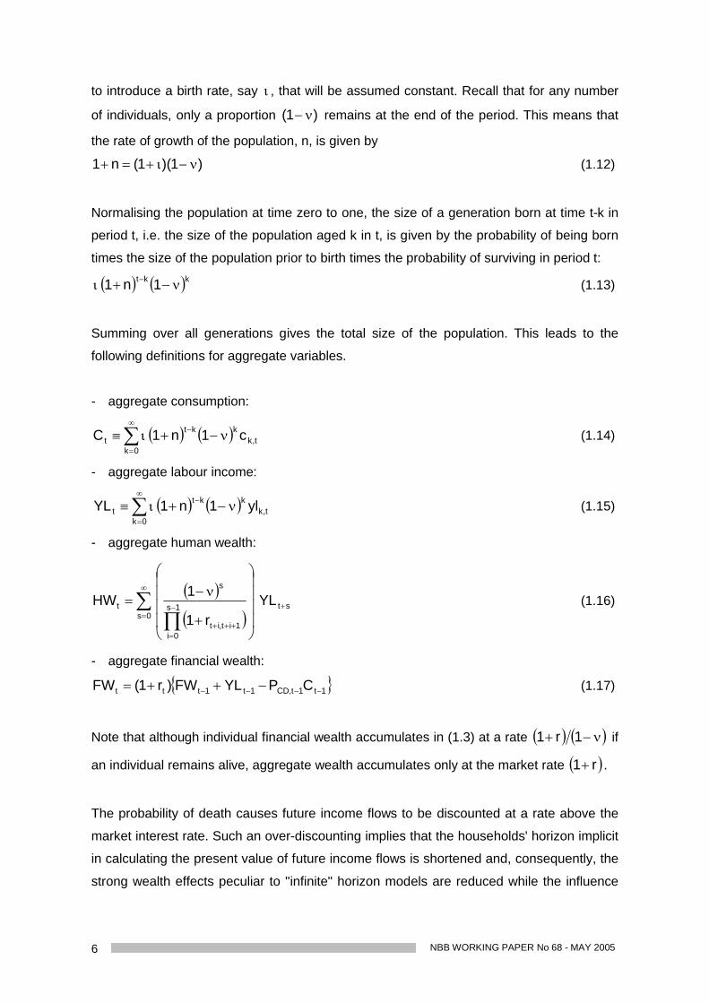
to introduce a birth rate, say , that will be assumed constant. Recall that for any number
of individuals, only a proportion )1( remains at the end of the period. This means that
the rate of growth of the population, n, is given by
)1)(1(n1 (1.12)
Normalising the population at time zero to one, the size of a generation born at time t-k in
period t, i.e. the size of the population aged k in t, is given by the probability of being born
times the size of the population prior to birth times the probability of surviving in period t:kkt 1n1 (1.13)
Summing over all generations gives the total size of the population. This leads to the
following definitions for aggregate variables.
- aggregate consumption:
0kt,k
kktt c1n1C (1.14)
- aggregate labour income:
0kt,k
kktt yl1n1YL (1.15)
- aggregate human wealth:
st0s
1s
0i1it,it
s
t YLr1
1HW (1.16)
- aggregate financial wealth:
1t1t,CD1t1ttt CPYLFW)r1(FW (1.17)
Note that although individual financial wealth accumulates in (1.3) at a rate 1r1 if
an individual remains alive, aggregate wealth accumulates only at the market rate r1 .
The probability of death causes future income flows to be discounted at a rate above the
market interest rate. Such an over-discounting implies that the households' horizon implicit
in calculating the present value of future income flows is shortened and, consequently, the
strong wealth effects peculiar to "infinite" horizon models are reduced while the influence

NBB WORKING PAPER No 68 – MAY 2005 7
of current income is strengthened. As a consequence, the extreme version of the
Ricardian equivalence does not hold since the present value of future tax changes does
not completely match current adjustments in tax payments.
Since the propensity to consume was independent of age, the aggregate consumption
function can now be written as:
t,CD
tt
t,CD
t1tt P
HWEPFW
rr111C (1.18)
which is the aggregate version of (1.9) and (1.10)
The estimation is based on a log-linear approximation of this consumption function in
which the proportionality of consumption to total wealth is ensured by imposing that the
coefficients of human and financial wealth sum to one:
tt,CDtt,CDtt rr2.1pfw05.0phw95.0c (1.19)
This life-cycle model determines the desired level of consumption. It depends on the one
hand on the financial wealth which equals the market value of financial assets. On the
other hand it also depends on human wealth which corresponds to the present value of
expected future labour income -defined net of taxes and inclusive of transfer payments-.
The magnitude of the coefficient on financial wealth is low as compared to that on human
wealth: a 10 p.c. increase in financial wealth only raises consumption by 0.5 p.c. against
9.5 p.c. for human wealth.
Finally, the optimal consumption is a negative function of a real short-term interest rate
reflecting intertemporal substitution in consumption, i.e. the effect the interest rate exerts
on the propensity to consume out of total wealth. Empirically, this negative sign is probably
also a consequence of the inclusion of durable goods in the consumption data. According
to the estimated coefficient, a 100 basis point cut in the annualised real rate would cause a
0.3 p.c. hike in desired consumption. If interest payments have a positive income effect,
they will be accounted for by the financial wealth variable which incorporates capital
incomes.
NBB WORKING PAPER No 68 - MAY 20058
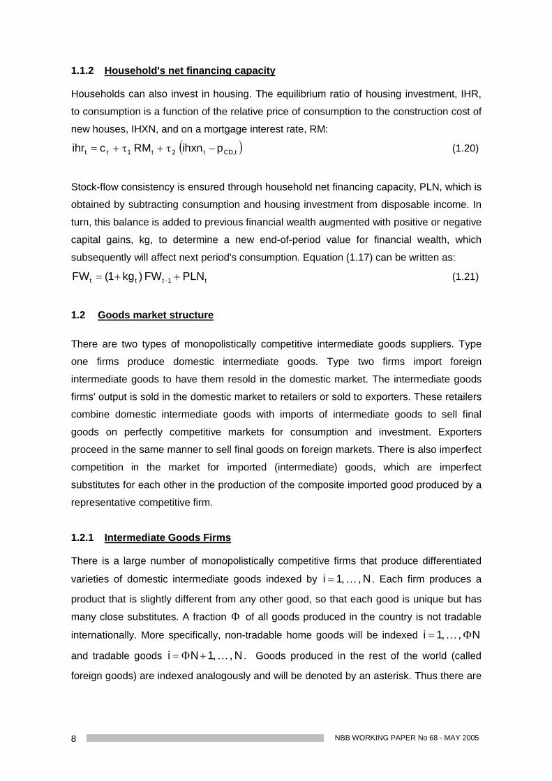
1.1.2 Household's net financing capacity
Households can also invest in housing. The equilibrium ratio of housing investment, IHR,
to consumption is a function of the relative price of consumption to the construction cost of
new houses, IHXN, and on a mortgage interest rate, RM:
t,CDt2t1tt pihxnRMcihr (1.20)
Stock-flow consistency is ensured through household net financing capacity, PLN, which is
obtained by subtracting consumption and housing investment from disposable income. In
turn, this balance is added to previous financial wealth augmented with positive or negative
capital gains, kg, to determine a new end-of-period value for financial wealth, which
subsequently will affect next period's consumption. Equation (1.17) can be written as:
t1ttt PLNFW)kg1(FW (1.21)
1.2 Goods market structure
There are two types of monopolistically competitive intermediate goods suppliers. Type
one firms produce domestic intermediate goods. Type two firms import foreign
intermediate goods to have them resold in the domestic market. The intermediate goods
firms' output is sold in the domestic market to retailers or sold to exporters. These retailers
combine domestic intermediate goods with imports of intermediate goods to sell final
goods on perfectly competitive markets for consumption and investment. Exporters
proceed in the same manner to sell final goods on foreign markets. There is also imperfect
competition in the market for imported (intermediate) goods, which are imperfect
substitutes for each other in the production of the composite imported good produced by a
representative competitive firm.
1.2.1 Intermediate Goods Firms
There is a large number of monopolistically competitive firms that produce differentiated
varieties of domestic intermediate goods indexed by N,,1i . Each firm produces a
product that is slightly different from any other good, so that each good is unique but has
many close substitutes. A fraction of all goods produced in the country is not tradable
internationally. More specifically, non-tradable home goods will be indexed N,,1i
and tradable goods N,,1Ni . Goods produced in the rest of the world (called
foreign goods) are indexed analogously and will be denoted by an asterisk. Thus there are

NBB WORKING PAPER No 68 – MAY 2005 9
*N1NN~ varieties demanded at home. The markets for internationally traded
goods are segmented by country, so that firms have the ability to set distinct prices in each
national market2. This last feature is typically called "Pricing To Market". Following Bergin
and Feenstra (2001) and Bergin (2003) the final goods retailers aggregate over the
differentiated goods with a translog functional form. Unlike the usual CES aggregator used
in most new open economy models, the translog specification does not restrict the
elasticity of substitution between goods to be constant but allows it to vary with the prices
of competing goods. When demand is elastic, -a feature necessary to have monopolistic
competition-, a fall in competing prices raises the elasticity leading to a pro-competitive
reduction in mark-ups. This feature is important in generating pricing-to-market also in
equilibrium3 since the demand curve faced by the firms has an elasticity that depends on
their price-setting decisions which may be different for their different markets, e.g.
domestic or foreign.
1.2.1.1 Domestic producers
a) Representative firm
The nominal price index is defined as the dual expenditure function of the final good
producers, which is assumed to have a translog form. This unit expenditure function is
defined by:
N~
1ijt
N~
1jitij
N~
1iitit PlnPln
21PlnPln (1.22)
where Pit is the home-currency price of good "i".
We consider the special case where all goods enter symmetrically
jifor1N~N~
,N~
,N~1
ijiii
The expenditure shares are obtained by differentiating the expenditure function
itjt
N~
)1j(1jit
tit Pln
N~Pln
1N~N~N~1
PlnPln
s (1.23)
2 This assumption can be justified with a system of selective distribution in which producers can choose theirdealers and prevent them from reselling to anyone but the end-users.
NBB WORKING PAPER No 68 - MAY 200510
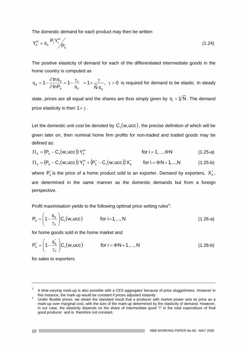
The domestic demand for each product may then be written
it
Htt
itHit P
YPsY (1.24)
The positive elasticity of demand for each of the differentiated intermediate goods in the
home country is computed as
0,sN~
1s
1Plnsln
1itit
ii
it
itit is required for demand to be elastic. In steady
state, prices are all equal and the shares are thus simply given by N~1s i . The demand
price elasticity is then 1 .
Let the domestic unit cost be denoted by ucc,wC t , the precise definition of which will be
given later on, then nominal home firm profits for non-traded and traded goods may be
defined as:
N...,,1iforYucc,wCP Hittitit (1.25-a)
N,...,1NiforXucc,wCPYucc,wCP *itt
*it
Hittitit (1.25-b)
where *itP is the price of a home product sold to an exporter. Demand by exporters, *
itX ,
are determined in the same manner as the domestic demands but from a foreign
perspective.
Profit maximisation yields to the following optimal price setting rules4:
N...,,1iforucc,wCs
1P tii
itit (1.26-a)
for home goods sold in the home market and
N,...,1Niforucc,wCs
1P tii
*it*
it (1.26-b)
for sales to exporters.
3 A time-varying mark-up is also possible with a CES aggregator because of price sluggishness. However inthis instance, the mark-up would be constant if prices adjusted instantly
4 Under flexible prices, we obtain the standard result that a producer with market power sets its price as amark-up over marginal cost, with the size of the mark-up determined by the elasticity of demand. However,in our case, the elasticity depends on the share of intermediate good "i" in the total expenditure of finalgood producer and is therefore not constant.

NBB WORKING PAPER No 68 – MAY 2005 11
The expenditure share can be substituted from (1.23) so that (1.26-a) can be solved for the
optimal price in terms of marginal cost and prices of competitors. This expression is
nonlinear, involving Pit and lnPit, so we will use an approximation to obtain a simple
solution for the price. In this simple linearised form, the price setting equation implies that
domestic prices for both traded and nontraded goods behave as
N...,,1iforp1N~
1ucc,wc1pN~
)ij(1jjttit (1.27-a)
where small case letters denote the logarithm of the variable and parameter 21
indicates the degree to which an individual firm's price setting decision is influenced by the
price of other competitors in the market, while the remainder is determined by its own
costs. And when goods are sold to exporters, their price is similarly given by
N,...,1Niforp1N~
1ucc,wc1pN~
)ij(1j
*jtt
*it (1.27-b)
b) Aggregation
To further simplify these price equations, consider the case of two equally-sized groups of
differentiated products at home and abroad, N = N*. The total number of products
demanded in the home country is thus N2 , a proportion 21 of which consists
of domestically produced intermediate goods. Let i,Hp denote the price of home goods sold
in the home market, Mjp the price of foreign goods sold in the home market. Then applying
expression (1.27-a) for all firms i = 1, ... , N and noting that in equilibrium Hi,H pp and
mtdpp MMj . Then assuming N is large one can solve for Hp as
ttHt mtd232
1ucc,wc232
21p (1.28)
Similarly denoting the price of home goods for the foreign market by ixtd , and the price of
foreign goods sold in the foreign market by *i,Fp and noting that in equilibrium xtdxtdi
and *F
*i,F pp , equation (1.27-b) may be compactly written as:
*Fttt p
32ucc,wc
3221xtd (1.29)

NBB WORKING PAPER No 68 - MAY 200512
This shows that firms set their price not only in response to changes in their own costs but
also in response to the prices set by their competitors. The relative weight depends on the
share of non-traded goods which determines the proportion of their competitors which are
foreign.
In linearised form, a definition of the price index for the domestic economy is
tHtt mtd21p
21p (1.30)
and domestic output sold in the home country is obtained by summing over the "domestic"
demand functions for all home goods i:
tHttHt dpp1
21y (1.31)
while exported output, xtr, is obtained in a similar manner
*tt
*tt d
21xtdp1
21xtr (1.32)
To obtain an expression similar to (1.30) for the foreign price index, consider a two-country
world. Then the foreign pricing-to-market and the relative price of non-tradables would be
the inverse of their home counterpart so that the foreign price index would be given by
t*Ft
*t xtd
21p
21p (1.33)
Thanks to this definition, the demand for exports can be expressed in terms of *Fp and xtd.
Using Y to denote production, market clearing for domestic intermediate goods requires
N...,,1iforYY Hitit (1.34)
N,...,1NiforXYY *it
Hitit (1.35)
Producing each variety of intermediate goods involves labour measured in hours, capital
and technical progress within a common CES production function with constant return to
scale:1
itKitLit K1LY (1.36)

NBB WORKING PAPER No 68 – MAY 2005 13
where 11 is the elasticity of technical substitution between labour and capital,
KL ,, are a share parameter, labour- and capital-augmenting technical progress
respectively5.
Static profit maximisation subject to the firm's production function (1.36) and to the derived
demand for the firm's output (1.24) yields the following FOC
it
itititit L
YPW (1.37.a)
it
itititit K
YPUCC (1.37.b)
where
ii
it
it
s11
is the gross mark-up;
1
itL
itL
it
it
LY
LY
; (1.38.a)
1
itK
itK
it
it
KY
1KY
(1.38.b)
Substituting equation (1.38.a) into (1.37.a) gives the optimal labour demand. Since it is
expressed in volume, i.e. total hours, in order to obtain employment we added a relation
for the average hours per worker. These are cyclical around a trend which is specified as
an increasing function of the ratio of full-time to part-time work and of conventional working
time.
Equations (1.37.b) and (1.38.b) determine the optimal demand for capital. Since the ratio
of long-run equilibrium investment (IOR) to target capital equals the sum of the
depreciation rate and the steady state growth rate of output (the latter being the sum of the
rate of technical progress,L
g , augmented with the rate of population growth, n), the
following steady state investment rate equation holds:
5 Note that without loss of generality we can assume that remains constant since, if 1, the precisevalue of is arbitrary and any change in it can be represented through biased technical progress which is
reflected in a change in the ratioK
L .
NBB WORKING PAPER No 68 - MAY 200514
nglnkiorL1tt (1.39)
This relationship shows the investment flow necessary to make the capital stock growing
at the steady state growth rate of the economy.
Knowing the optimal factor demands, real unit production cost is given as1
KL
R ucc1w)ucc,w(c (1.40)
This is the minimum cost of obtaining the unit output level given that the "real" unit input
prices are w and ucc. This function is homogenous of degree one so that the nominal unit
cost is simply given by )ucc,w(cP)ucc,w(C R
1.2.1.2 Importing firms
The importing firms choose their resale price in our home market Mjtp to maximise their
profitsMjt
*Fjt
Mjt
Mjt YPP (1.41)
where the cost of imported intermediates in domestic currency is given by the price of
foreign goods sold in the foreign market *i,Fp .
Profit maximisation implies
N,...,1NjforPs
1P *Fjt
jj
MjtM
jt (1.42)
and substituting for the expenditure shares from (1.23) and following the same steps as for
domestic goods in (1.28), one finally gets
Ht*Ftt
Mt p
32p
3221mtdp (1.43)
From (1.43) and (1.28), we can obtain a price index for intermediate goods sold on the
home market in terms of unit cost and foreign price
*FttHt p
21
21ucc,wc
21
211p (1.44)

NBB WORKING PAPER No 68 – MAY 2005 15
Comparing (1.44) to (1.29), rather than to (1.28) highlights more clearly how prices
charged by home firms in the domestic and export markets can be different.
1.2.2 Production of final goods
The composite final goods, Z, are obtained by aggregating over intermediate home goods
along with aggregating over imported goods6:1M
tHtt YYZ (1.45)
where HY is an aggregate of the individual home goods sold in the domestic economy,
HiY and MY is an aggregate of the imported goods, M
iY .
Final goods producers (or aggregators) behave competitively, maximising profits each
period, taking the price i,HP of each intermediate home good HiY and the price, imtd , of
each imported foreign goods, MiY ,as given:
Mtt
Htt,Htt
Zt YmtdYPZP (1.46)
where P is the overall price index of the final goods, HP , the price index of home goods
and mtd, the import price of foreign goods. Given the aggregation function defined
in (1.45), the conditional aggregate demand for home and foreign goods will be
t
1
t
t,HHt ZP
PY (1.47)
t
1
t
tMt ZP
mtd1Y (1.48)
with the demand for individual goods given by (1.24) and its analogues for imports. The
home price index may be written as1
tHt1
t mtdP1P (1.49)
which in log-linearised form is the analogue to (1.30) with 21 .
This could in principle be the end of the story. However, since we are interested in a
decomposition of aggregate demand in expenditure categories, we will consider that the
composite final good is then transformed without cost into differentiated goods which are
6 A CES aggregator is often use in the literature. However since this approach will serve for eachexpenditure categories it is assumed that the elasticity is unitary for all categories. Due to a lack of data onthe various categories of both import quantities and prices, it seems hazardous to try to identify eachelasticity of substitution between domestic and imported categories of goods.

NBB WORKING PAPER No 68 - MAY 200516
either sold as consumption goods, investment goods, housing investment and government
goods to final goods aggregators. The exporters proceed in the same way so that the
demand for home good results from the sum:
t,Ht,Hh
t,Ht,Ht,HHt XGIICY (1.50)
where t,Ht,Hh
t,Ht,Ht,H X,GI,I,C denote the amount of domestic goods used in the production
of consumption, investment, housing investment, government purchases of goods and
services and exports respectively. These demands are obtained by aggregating the
individual demand (1.24) for each specific category. Proceeding along the same line for
imports we obtain aggregate imports as:
t,Mt,Mh
t,Mt,Mt,MtMt XGIICMTRY (1.51)
For instance, for consumption, replacing Z by PCR, HY by HC and MY by MCCC 1
t,Mt,Ht CCPCR (1.52)
where t,MC refers to imported consumption goods. The aggregator sells the final good to
households at a price PCD,t which may be interpreted as the consumption price index. Profit
maximisation implies the following (log)price indice:
tC
t,HCi
tt,CD mtd1pt1lnp (1.53)
where itt stands for indirect taxes (less subsidies) rate.
This demand will be allocated between home and foreign goods according to
t
1
t,CD
t,HCt,H PCRP
PC (1.54)
t
1
t,CD
tCt,M PCRP
mtd1C (1.55)
Production of the final investment goods, IOR, and of government purchases of goods and
services, GCR1, are modelled analogously. Finally, exporters also combine traded
domestic intermediate goods and imported brands to produce export goods, XTR.
Therefore, we have the analogues to (1.53), (1.54), (1.55) for each GDP category with
specific weights for domestic and imported goods reflecting information from input-output
tables.
NBB WORKING PAPER No 68 – MAY 2005 17
From (1.49) and (1.53), it can be seen that the domestic and foreign price are common
across final expenditure categories. Consequently, differences in their respective deflator
will only reflect the differences in their import share.
Note that, in line with available input-output tables, housing investment is produced from
domestic materials only, i.e. 0IhM .
1.2.3 Aggregate imports
Substituting for the import demand by categories of expenditures, (1.51) becomes:
t
1
t,TD
t,TDX
t
1
t,1CD
t,TDGt
1
t,OD
t,TDIt
1
it
t,CD
t,TDCt
XTRXM
)1(
1GCRGM
)1(IORIM
)1(PCR
t1PM
)1(MTR
(1.56)
where XGIC ,,, are the share of home produced goods in private consumption,
investment, public procurement, GCR1, and exports respectively, which can be derived
from input-output tables.
This section has described the central role played by the price of home domestic
intermediate goods (also labeled price of domestic output) in the derivation of the main
deflators of final demand. A comparison of the empirical versions of the price set by
domestic firms on the home and foreign markets indicates the degree to which firm's price
setting decision is influenced by the price of competitors in that market:*FttHt p51ucc,wc54p
*Fttt p31ucc,wc32xtd
Not surprisingly home firms are more sensitive to competitors' prices on the foreign market
than on the domestic market. Since imported goods compete with domestic ones, the price
set by importers is also an average of their own costs, represented by the price they have
to pay to acquire the foreign goods, and of the price of domestic intermediate goods:*Ftt
*FtHtt p1511ucc,wc154p32p31mtd
These relationships show that exchange rate pass-through is far from complete even in the
long term because modifications of importers' mark-ups partially offset exchange rate

NBB WORKING PAPER No 68 - MAY 200518
changes. On top of that, the composition of *Ftp , which is an indicator of the price of both
intra- and extra-euro area competitors, reinforces this incompleteness of the pass-through.
In order to account for the different expenditure categories, the final demand has been
subdivided into private consumption, business investment, government procurement and
exports, all of which have a domestic and an imported component, housing which is made
of domestic inputs only and inventories which are exogenous.
Finally, from the production function and the factor demands, we have obtained the labour-
augmenting technical progress and the elasticity of substitution between capital and
labour. The former is supposed to grow at a rate around 1.5 p.c. a year and the estimate of
the latter is close to 0.5. A low elasticity of substitution helps somewhat to match the
empirical findings of a small response of business investment to interest rate changes
since it lowers the response of capital formation to variations in the user cost. In addition,
with an elasticity of substitution below one, capital accumulation creates employment while
growth in the labour supply and the labour-augmenting technical progress will cause a rise
in unemployment unless they are offset by increased investment.
1.3 Labour market structure
In Belgium, the government has intervened quite regularly in the course of the wage
formation process. This may be a source of concern when trying to analyse that process
econometrically. However, for simulation purposes, we will consider that in the long run
wages can be explained according to a bargaining model between firms and unions and
that, in practice, the correction mechanism is not market determined but sometimes
imposed by government interventions. Of course, forecasting exercises need to respect
the law of July 1996 for the promotion of employment and the safeguarding of firms'
competitiveness which guarantees that the principle of automatic indexation of wages to
the “health” consumption price index is maintained but that nominal wages do not grow
faster than the weighted average wage growth in France, Germany and The Netherlands.
Note that oil, tobacco and alcohol are excluded from the basket used to calculate the
"health" consumption price index. This feature may be important in understanding the
transmission of oil price shocks. In the rest of the model, the labour supply is treated
exogenous.

NBB WORKING PAPER No 68 – MAY 2005 19
Each intermediate good firm negotiates wage with a single union according to a "right to
manage" bargaining model. By organising themselves in trade unions, households can
extract some producer surplus. Once wages are fixed, the firm decides on employment
according to its labour demand curve (1.37.a). Each representative union seeks to
maximise the average real "consumption" income of "insiders" which is equal to
CD
ii
Niii P
AS1WSV (1.57)
where Si is the proportion of insiders who will keep their job following the wage settlement
which will yield the wage NiW and Ai is the reservation wage or expected income for those
who will lose their job. Actually, the relation between gross nominal wage, WB, net real
"consumption" wage, WN, and real "producer" wage cost, WC , are given by
H
1wB
C
Pt1WW and
CD
3w2wB
N
Ptt1WW and the "tax and price wedge" is given
by NC
WWz . In these formulae, the average tax rates 3w2w1w t,t,t refer respectively to
the social security contributions of employers, of employees and withholding tax on earned
income. The expected nominal income available outside the firm is assumed to be an
average of the wage in other firms, 3w2wB tt1W , and of the unemployment benefit,
B:
uBtt1Wu1A 3w2wBe
(1.58)
where u is the unemployment rate and is a constant.
The outcome of the bargaining process is the wage rate that maximises a Nash product of
the type,
iiiii VV (1.59)
where is an index of relative bargaining power, and V and are the utility functions of
the unions and firms respectively. The bar above a variable indicates the outside options
available to the parties if negotiations collapse and the firm shuts down. It is assumed that
0,PAV iCD
i .
Then the Nash product can be rewritten as
i1wBii
CD
3w2wBi
i t1WSP
Att1W(1.60)
NBB WORKING PAPER No 68 - MAY 200520
with Si assumed to depend on the wage cost. The product is maximised (by choosing BiW )
when
iL
ik
tSN
3w2wBi
3w2wBi
i
i1wBi
LK1
1Att1W
tt1WLt1W (1.61)
where SN is a constant reflecting the vulnerability of insiders to job loss.
From the definition of alternative income (1.58), it follows that
3w2wB
3w2wB
BBi3w2w
3w2wBi
3w2wBi
3w2wBi
tt1Wtt1W
B1u)WW(tt1
tt1WAtt1W
tt1W
e
(1.62)
In a symmetric equilibrium all intermediate goods firms and unions make identical
decisions so that
N/KK,N/LL,SS,PP,WW iiiHHiBB
i ,for all i = 1, ..., N
Thus one gets
3w2wB
3w2wB
3w2wB
tt1WBbwhere,
b1u1
Att1Wtt1W
(1.63)
Combining (1.59) with the fact that the profit rate is given by
tH
1YP
(1.64)
yields a relationship that, in case 0SN , simplifies to
b1u1
YPLt1W t
H
1wB
(1.65)
NBB WORKING PAPER No 68 – MAY 2005 21
Note that 0SN means that higher wages will have no effect on the employment of
insiders although they will reduce the jobs available to outsiders7.
Making use of the production function to eliminate L/Y, one finally gets the aggregate wage
equation8:1
t
1L
H
1wB
b1u
u1k11
Pt1W
(1.66)
where PLLF
Kk , LFP being private labour force.
This relation shows that if k falls following a faster growth in the labour supply or a slower
growth in the capital stock, the real production wage should also fall to prevent
unemployment from rising.
Log-linearising equation (1.66) yields the following equilibrium wage setting rule for the
economy:
t
ttttt,L
Ct u1
k1log1b1loguloglog1loglogw
(1.67)
From the definitions of WC and WB, one can see that employer social security contributions
have a direct one for one impact on wage cost while employee's contribution and income
taxes exert their effect through the replacement ratio.
Estimation of (1.67) results in the following relation:
t
ttttt,L
Ct u1
k1log1ulogb2.018.01log05.0logw
7 Actually it can be shown that when demand is non stochastic, as it is the case here, SN equals either 0 or1. Intermediate cases occur when demand is stochastic.
8 Alternatively in (1.65), one could have expressed WL/PY in terms of k, u, ... and obtained an implicit
equation for equilibrium unemploymenttt
*t
tt
*t b1
u1
k11
u
This relation emphasises that the equilibrium unemployment rate is dependent not only on labour marketconditions such as union power, , or the replacement ratio, b, as in Layard et al. (1991) but also thecapital-labour ratio, k, and the (inverse) mark-up through which changes in foreign prices will pass.
NBB WORKING PAPER No 68 - MAY 200522
It shows that the real producer wage follows trend labour productivity but can deviate from
it due to:
- rent sharing: although the estimated coefficient at 0.05 is far below 1 as implied by
theory;
- changes in the rate of unemployment and in the replacement ratio. Given that wage
formation has not always been determined by market forces, it is not surprising that the
empirical impact of these two variables is also lower than theory would predict. Actually,
the replacement ratio dampens the already mild effect exerted by the rate of
unemployment. When unemployment benefits are high as compared to pocket wages,
the negative impact of unemployment is reduced;
- the last term on the right-hand-side. To illustrate how this term, which would not be
present under a Cobb-Douglas production function, works. Imagine that for some
reason capital is growing slower than the labour supply and that k is falling. To maintain
a constant unemployment rate under these circumstances, the real wage cost must
grow less than trend productivity or, in other words, the real wage in efficiency units
must fall.
1.4 Government
Many variables in this sector are either exogenous in real terms or defined through
technical relations. Current expenditure is divided into interest payments on government
debt and different types of primary expenditure categories. The allocation of the
outstanding debt over long term and short term domestic currency and foreign currency
debt is taken as given and a representative interest rate is applied to each corresponding
debt category. The weighted sum of these representative rates is, in turn, used to estimate
the implicit rate on government debt. In modelling primary expenditure, the following main
items are distinguished:
- government wages and pensions are indexed according to the “health” CPI, real wages
being treated exogenous;
- government consumption of goods and public investment are exogenous in real terms
and the deflator of the former follows both the price of home produced goods, with a
weight of G , and of imported goods with a weight of G1 as explained in (1.49)
while the deflator of the latter is related to the private sector investment deflator;
- most transfers to households are exogenous in real terms but are indexed to the
“health” CPI. Unemployment benefits are the only business cycle sensitive component.

NBB WORKING PAPER No 68 – MAY 2005 23
In the long run, we have to ensure that the debt to GDP ratio settles down to its steady
state value. To achieve this goal, total transfer payments to households are used as the
control variable. One possibility would be to incorporate a fiscal policy feedback rule that
would adjust transfers to bring the debt to GDP ratio to its desired level. Such a
convergence could be achieved by specifying a fiscal rule which imposes a targeted path
for the debt and/or deficit ratios. Such a rule is highly pro-cyclical since in order to keep the
debt or deficit ratio on target when output is below trend, the deficit must also be lower
than in steady state, which reinforces the reduction of output. Therefore, to avoid too much
cyclical variation when simulating the model with a fiscal rule, we make use of a more
flexible rule which only guarantees that the debt ratio decreases at a given rate but does
not strictly respect a given level; i.e. it accommodates shocks but ensures convergence to
the steady state, the exact date of the convergence being different from shock to shock.
General government receipts have been split into
- direct taxes on households' earned income: due to the progressiveness of income
taxes, the average tax rate is a log-linear function of the income level per head. The
nominal income level is affected by both a price and a real component. Under normal
circumstances, tax brackets are indexed to the rise in the consumption price of the
preceding year and then price level changes do not change the average tax rate. In
addition the average tax rate can also reflect changes in the tax structure;
- direct taxes on companies: the tax amount is explained by the firms' tax rate, which is a
flat one, together with the taxable base which is represented by the gross operating
surplus of companies;
- social security contributions are split into employers', employees' and self-employed
contributions. In each case implicit contribution rates are modelled as functions of the
official rates;
- indirect taxes are estimated as an aggregate of VAT and excises duties and the taxable
base is nominal private consumption and housing investment.
Government debt is determined by the government budget constraint which says that debt
(GDN) equals previous period debt minus budget surplus (GLN):
GDN = GDNt-1 -GLN (1.68)
NBB WORKING PAPER No 68 - MAY 200524
1.5 Monetary and financial sector
Monetary policy is exogenous to the model so that whatever the outcome of shocks in
terms of inflation the monetary policy stance, as measured by the nominal rate, will remain
unchanged. There is no role for monetary aggregates in determining prices and output.
Monetary policy affects model results through the interplay of interest rates. The model
includes a 3-month interest rate, a long term bond rate, a mortgage rate and a rate for
credit to companies.
1.6 Steady-state
The steady state growth rate of the model can be summarised as follows.
For real variables, define
ty1t yg1y (1.69)
where yg , the equilibrium real growth rate of the economy, is derived from differentiating
the production function (1.36) with respect to time:
KLgg
KY1gg
NLYg K
KL
Ly (1.70)
which can also be written as
KLgg
NLK1ggg
NLY
KL
KLy
L(1.71)
or making use of the production function
KLgg
NLYggg
NLY
KL
LyL
(1.72)
Hence
KKLgggggg
NLYg KKLL
y (1.73)
Finally, making use of (1.37.a) and denoting the share of wages by Ls , this simplifies to
KKLggggggs1g KKLLy (1.74)

NBB WORKING PAPER No 68 – MAY 2005 25
Along a balanced growth path, if technical progress is purely labour-augmenting 0gK
,
the real growth rate of the economy equals the growth rate of labour in efficiency unit
provided that the capital stock also grows at that rate.
Rowthorn (1996) also shows that contrary to the Cobb-Douglas technology used in Layard
et al. (1991), this condition also affects the unemployment rate in equilibrium. He shows
that u* evolves through time according to:
KLggggif0
dtdu
LK
*
(1.75)
This gives the growth rate of physical capital required to offset the combined effects of
labour supply growth and biased technical progress. Unemployment remains constant if
capital grows at this rate, also called the "natural" rate of growth.
Note that it's the model's focus on consistent expectations that necessitates that more
attention be given to equilibrium properties than is the case in traditional macro models.
Solving forward looking models requires imposing terminal conditions that pin down
agents' expectations beyond the simulation horizon. It is then natural to determine such
end-points by making use of the model's steady state growth rates9.
9 While the steady-state growth rates are known and are invariant to shocks affecting the economy - otherthan shocks affecting directly the steady state growth rate itself-, the steady-state levels are conditional totheir history in the simulations.

NBB WORKING PAPER No 68 - MAY 200526
1.7 Long run parameterisation
The long run parameterisation is summarised in table 1.
Table 1 - Long Term Parameters
Parameter Value Source
technical progressL
g 0.00385 estimated
labour supply growth n 0.0013 sample meanelasticity of substitution 0.52 estimatedlabour share in production 0.80 fixedprobability of death 0.035 fixedshare of non-traded 0.41 sample meandemand price elasticity 5 fixedgross mark-up 11 0.25
share of home goods in:- consumption C 0.32 input-output
- business investment i 0.74 input-output
- government procurement G 0.13 input-output
- exports X 0.63 input-output
inflation inflation 0.00475 fixeddebt-to-gdp ratio gdn/(yen*4) 0.60 growth and stability pact
The real growth rate of the economy is given by the estimated labour-saving technical
progress augmented with the average rate of growth of the labour supply. The former
results from the estimation of the demand for labour and its value is 0.385 p.c. per quarter.
For the latter, we assumed that no further reduction in conventional working time will occur
and that it equals its average over 1980-2003, i.e. 0.13 p.c. per quarter. In calibrating the
steady-state we also assumed that inflation is close to 2 p.c. per year, i.e. 0.475 p.c. per
quarter. The elasticity of substitution between labour and capital, , comes from the
estimation of the demand for production factors and is estimated at 0.52.
In evaluating human wealth from the future stream of labour income, we will use a
probability of death of about 3.5 p.c. This is quite high and, when the discount process with
the real rate of interest is also taken into account, this means that the first 5 years count for
75 p.c. in the present value sum of future incomes.
From the definition of demand elasticity under symmetry and since in a steady state all
firms with the same cost charge the same price and thus have the same market share, the
elasticity of demand may be written as 1 which implies a steady-state mark-up over
NBB WORKING PAPER No 68 – MAY 2005 27
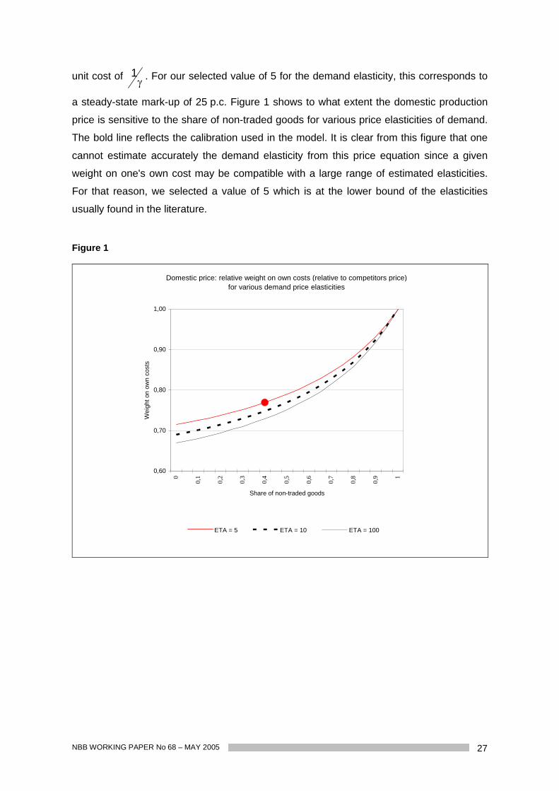
unit cost of 1 . For our selected value of 5 for the demand elasticity, this corresponds to
a steady-state mark-up of 25 p.c. Figure 1 shows to what extent the domestic production
price is sensitive to the share of non-traded goods for various price elasticities of demand.
The bold line reflects the calibration used in the model. It is clear from this figure that one
cannot estimate accurately the demand elasticity from this price equation since a given
weight on one's own cost may be compatible with a large range of estimated elasticities.
For that reason, we selected a value of 5 which is at the lower bound of the elasticities
usually found in the literature.
Figure 1
Domestic price: relative weight on own costs (relative to competitors price)for various demand price elasticities
0,60
0,70
0,80
0,90
1,00
0
0,1
0,2
0,3
0,4
0,5
0,6
0,7
0,8
0,9 1
Share of non-traded goods
Wei
ght o
n ow
n co
sts
ETA = 5 ETA = 10 ETA = 100

NBB WORKING PAPER No 68 - MAY 200528
2. DYNAMICS
2.1 Theoretical considerations
Equilibrium equations are first derived and subjected to coefficient restrictions from static
economic theory according to section 1. They take the following form:p
j jtj0*t Zy (2.1)
where yt* is the decision variable10 of interest and Zj are its p explanatory variables. These
equilibrium paths for the decision targets describe the relationships between variables
when all dynamic adjustments have been accomplished.
Of course, the current state of these variables should not necessarily reflect equilibrium at
all points in time. It is therefore necessary to embed the equilibrium conditions into
dynamic equations describing their law of motion towards these equilibrium paths. Many
macroeconomic models incorporate deviations from equilibrium in unrestricted error
correction equations:
t,j
p
1jj1t
*1t1tot Z)L(by)L(a)yy(µcy (2.2)
where a(L) and b(L) are unrestricted polynomials in the lag operator added arbitrarily. Such
equations may deliver nice empirical fits of the data but they are not apt for a coherent
analysis of responses by rational agents reacting to news about future events. Indeed,
dynamic behaviour does not solely originate from delayed responses due to the costs of
adjusting variables, but also from movements induced by changes in agents' expectations
about future events. To answer policy related questions appropriately, agents'
expectations need to be identified. Therefore, treating expectations explicitly in estimating
dynamic equations should permit to identify frictions that impede dynamic adjustments and
expectations separately.
As explained in Jeanfils (2000) in order to obtained richer dynamics than the one resulting
from quadratic adjustment costs we are using Polynomial Adjustment Costs (PAC). This
generalisation of quadratic adjustment costs is due to Tinsley (1993). Only a brief
description of his approach is presented hereafter11. Consider the following loss function:
10 In what follows, the terms 'decision variable', 'target' and 'equilibrium level' are used as equivalents.11 For a more exhaustive treatment of what follows, see Tinsley (1993) and Kozicki and Tinsley (1999).

NBB WORKING PAPER No 68 – MAY 2005 29
2
itk
m
1kk
2*itito
oi
itt yL1byybEC (2.3)
The first squared term represents the disequilibrium cost while the second represents
adjustment costs and is a fixed discount factor. This decision rule relaxes the assumption
that it is costly to adjust only the level of the decision variable (k=1) and introduces costs in
modifying differences in the variable: the rate of growth of y corresponds to k=2, the rate of
acceleration to k=3, etc. Minimisation of this loss function yields the Euler equation
0}y)L1)(L1(byy{E tk1
m
1kkt
*tt (2.4)
or with another notation
0y)...1)(...1(
y)L...L1)(L...L1(E
t*
m1m
m1
tm1mm
m1
1t (2.5)
A solution to this Euler equation well-suited for estimation is given by the following decision
rule:
te*ity1tEma,,
0i iSity*ia
1m
1i)*
1ty1t(y1Aocty (2.6)
where Si is the multiple-root discount factor, which is analogous to the inverse of the
unstable root in the case of costs affecting only the level. They are non-linear functions of
the discount rate and of the m parameters of the lag polynomial A(.), written compactly
as 'a'. Expectations of changes in the target, Et-1 yt+i *, are provided by an auxiliary VAR
as in (2.2). Since the extent of these frictions (the size of m) is estimated rather than
imposed by an a priori choice of a particular adjustment cost function, the empirical
goodness-of-fit of the dynamic model equations is far better than those obtained from
usual Rational Expectations models and is comparable with time series models. In
particular, high residual autocorrelation which is generally present in empirical tests of
decision rules based on level adjustment costs, is strongly reduced.

NBB WORKING PAPER No 68 - MAY 200530
Optimal adjustment today ty depends on three factors: (i) the deviation of last period's
level from its equilibrium *1t1t yy , (ii) past changes in y12, (iii) a weighted forecast of
future changes in equilibrium or target levels *ity for which the forecast weights Si are
declining in time since they are functions of the discount factor (i.e. forecasts far in the
future are less important than the forecast for tomorrow). It is the introduction of multiple
lagged changes in y that enables to have a better fit for the dynamic behaviour of most
macroeconomic variables than fits obtained in former empirical implementations of rational
expectations.
2.2 Estimation
Estimation of (2.6) requires a three-step process since its coefficients are complicated
nonlinear functions of both the parameters in the forecast model and the parameters in the
adjustment cost polynomial. First, coefficients in the definition of the targets y* are
estimated in a cointegration framework or imposed from theoretical restrictions, cfr.
Table 1. Then a forecasting VAR model for y* is estimated. And finally the coefficients ai*
are estimated. Since the dynamic equation (2.6) is linear in variables, its nonlinear
coefficient restrictions present in the forward weights Si can be imposed with an iterative
Least Squares procedure that, at each iteration, restricts the coefficients in Si to values
determined by estimates of the adjustment coefficients from the prior estimation13. In all
cases, the value of has been fixed to 0.9514.
Households' decisions concerning consumption and residential investment and domestic
firms' decisions (labour demand, investment, and prices) as well as exporters' and
importers' pricing rules have been modelled in the polynomial adjustment costs framework.
As an illustration of the results, the firms' pricing decision rule for domestic intermediate
goods is given by:
)0i
p(SEp0.676(0.078)
)p(p0.122(0.023)
p iHti1-t1-Ht1Ht1-HtHt (2.7)
12 These lagged terms are not present if agents minimize only the costs associated with changing the level ofy which was the assumption made in earlier applications of rational expectations models as estimated from(42) and (44). The parameter ai* are the coefficients of the lag polynomial A*(L) implicitly defined by A(L) 1-L+A(1)L-A*(L)(1-L)L.
13 The order of adjustment costs, m, is chosen empirically by testing for the number of significant lags of thedependent variable in an unrestricted ECM. Note that this procedure does not correct for possiblegenerated regressor bias.
14 Estimation results are not very sensitive to small variations in ,e.g. from 0.95 to 0.98.

NBB WORKING PAPER No 68 – MAY 2005 31
This equation contains a significant error-correction term (standard deviations are given in
parentheses) and one lag in output price inflation, meaning that inflation exhibits some
persistence. In addition, it is augmented with expectations of the target for which the sum
of weights equals 0.35515. Grouping all leads gives the following compact notation:
)p(Eleads355.0plags676.0)p(p0.122p iHt1-t1-Ht11Ht1-HtHt (2.8)
Table 2 - Compact view of equations
Order ofadjustment
cost (m)
Mean lead ofexpectations
of targets
Meanlag
LR test forREH1 Additional dynamics
Households
Consumption 3 1.7 1.6 0.64 Changes inemployment
Investment in dwellings 4 1.1 1.1 0.92
Firms
Labour 1 4.0 5.4 0.42 Investment 3 4.4 5.6 0.79 Accelerator + cash flow Domestic price 2 2.2 2.0 1.00 non linear output gap2
Exporters and importers
Export price 2 2.1 2.5 0.03 non linear output gap2
Import price 1 1.7 1.9 0.01 non linear output gap2
1 LR test (p-value) of excluding Var determinants of expected target changes, y e* . A p-value of 0.05 or less indicatesa rejection of REH restrictions with at least a 95 p.c. level of confidence.
2 defined as the ratio of actual output growth to the steady state rate of growth.
Table 2 summarises the results obtained for the seven equations mentioned above.
Column 1 gives the order of adjustment costs, m, ranging from 1 to 4. Column 2 reports
the mean lead of expectations of the targets. This is a compact measure of how far ahead
agents tend to look as well as how quickly a variable adjusts to expected future events. In
principle, agents plan over an infinite future, but the effective length of the planning period
is determined by the extent of the frictions. Actually, a quick adjustment is associated with
a short expectation horizon. Column 3 gives the mean lag of the series. This is a measure
of the average speed of response to past events. As shown in this table, consumption,
housing investment and prices exhibit mean leads and lags of two quarters or less
apparently reflecting the ability of households and price makers to adjust their decisions
variables quickly. Labour shows that a low order in a variable's polynomial adjustment cost
function does not necessarily imply a low mean lead or lag of its series. Column 4 of
table 2 provides a Likelihood Ratio test of the rational expectations over-identifying
15 Some diagnostic tests for the dynamic specification of the equations are given in appendix A2.

NBB WORKING PAPER No 68 - MAY 200532
restrictions on the coefficients of the agents' VAR forecast model. If the additional
regressors are statistically significant, it implies that the p-values are low which means that
households or firms do not have rational expectations as defined by the VAR's forecasts in
their dynamic adjustment equations. As shown by their p-values, these restrictions are,
with the exception of import and export prices, never rejected at conventional levels of
significance16.
16 In the unrestricted equation used in the LR test, the same lags of the variables included in the VAR areintroduced as additional regressors.

NBB WORKING PAPER No 68 – MAY 2005 33
Figures 2, 3 and 4
Distributions of weights in firms' decisions
-0,0500
0,0000
0,0500
0,1000
0,1500
0,2000
Quarters
Domest ic priceLabourInvestment
Distributions o f weights in househo lds' decisions
-0,2000
-0,1000
0,0000
0,1000
0,2000
0,3000
0,4000
Quarters
Consumption
Housing Investment
Distributions of weights in exportand import prices
0,0000
0,0500
0,1000
0,1500
0,2000
0,2500
Quarters
Export priceImport price

NBB WORKING PAPER No 68 - MAY 200534
Figures 2, 3 and 4 present the distributions of weights, i.e. the contribution of past and
future expected changes in the target on current decisions. The optimal current level of a
variable, x, given the presence of frictions can be represented as a two-sided moving
average of past and future target values, x* :i
*iti1tt xEx . The weights depicted in
figures 2, 3 and 4 sum to one for each variable. Weights for past quarters, shown to the left
of the peak, indicate the importance of past equilibrium levels to current decisions. Since,
as the quarters go by, older plans are revised or reach completion, the weights for past
planning periods tend to zero. In the same way, the weights of future targets shown to the
right of the peak diminish with the time horizon because of discounting and because more
distant plans can be corrected if necessary by taking other measures in future quarters.
Since long mean lead and lag are reflected in a rather flat curve, two types of weights
distributions appear. One shape, exemplified by labour, investment and domestic output
price, tends to be relatively flat, reflecting a strong influence of planning considerations in
the evolution of the variables. The other shape which is more concentrated around the
peak concerns households, exporters and importers. In particular, import price and
housing investment react very quickly and there is a dampening cycle in the evolution of
the latter series.
2.3 Wage Dynamics
In section 1.3, the optimal wage rate for a given period has been derived. However, wage
contracts are not set continuously because, once signed, they will not be revised for
several periods. In order to reflect this feature, we follow a simplified version of Dotsey,
King and Wolman (1999) state dependent pricing model which boils down to a time
dependent formulation. Assume that wages, once bargained, are set for up to a maximum
time period J (J>1). This is different from Taylor's staggered prices (1980) in which wages
are set for exactly J periods and from Calvo's model (1983) in which J is infinite. At the
start of each period, there is a fraction J,...,2,1jjt of each vintage of contracts which
has not been adjusted for j periods and thus remains equal to Cj-tw . Let i denote the
probability that a contract is adjusted conditional on having remained in effect for i periods.
The probability of non-adjustment is thus i1 . The total fraction of wages which is
adjusted is equal to it
J
1iit0 and comparably a fraction jtjjt 1 in each

NBB WORKING PAPER No 68 – MAY 2005 35
category j = 1, 2, ..., J which remains equal to the wage bargained j periods ago. These
fractions are related to the start-of-period fractions by
jt1t,1j for j = 0,1, ..., J-1 (2.9)
so that
1t,1jjjt 1 for j = 1, ..., J-1 (2.10)
Since all wages must be into one of the categories in terms of time span since their last
change:1J
1iitt0 1 (2.11)
Then a fixed weight aggregate wage index can be calculated as
jtj
J
1jjtj
J
1jj w1w (2.12)
The average contract length is given by
j1DJ
1j
1J
0hhj (2.13)
Note that in a model à la Calvo the proportion of wage contracts that are modified each
period is Jandj,j . The fraction of contracts that have not been adjusted
is 1jj 1 and is decreasing in j (i.e. there will be a maximum of contracts
changed after one period).
The estimation of the wage equation is done in two steps. First, we estimate a "flexible"
version of the log-linearised optimal wage equation and then the dynamics. For this
second step, one needs to choose a maximum contract length J prior to estimation. In
addition, one also needs to estimate the J conditional wage change probabilities, j . This
may be simplified by adopting the same non-linear functional form as Murchinson et al.
(2004) which allows one to reduce the number of free parameters:
1J...,,2,1j;01
1jJ
j (2.14)

NBB WORKING PAPER No 68 - MAY 200536
where is a (positive) parameter to be estimated and it ensures that the conditional
probability of changing wage is increasing with time since the last wage change at an
increasing rate ( 0j,0j 2j
2j ).
Note that wages are bargained on a real gross basis and that the government often
intervenes to affect wage costs by changing tw1, the employers' social security contribution
rate. In addition, there is automatic ex-post indexation that comes in addition to the
bargained wage. The resulting wage index can be written as:
Lg.jp1ww
1j
0qqtjt
1J
1jjtj
J
1jj (2.15)
The average contract length in (2.13) can be written as
jomegaDJ
1jj (2.16)
We choose a maximum contract length, J, of 8 quarters and the resulting estimated is
then equal to 0.37. This gives an average contract length, D, of 4.1. Figure 5 shows the
distribution of the contract lengths represented by the omega's in (2.16) and compares it to
the distribution of Calvo contracts, that results in the same average contract length
( 24.0 ).
Figure 5
Distribution of contracts lengths(average duration = 4.1)
0
0,05
0,1
0,15
0,2
0,25
0,3
1 2 3 4 5 6 7 8
omega (xhi=0.37) Calvo omega
NBB WORKING PAPER No 68 – MAY 2005 37
2.4 Price Dynamics
Apart from domestic intermediate goods, exports and imports prices that result from
dynamic optimisation, the dynamics of consumption, investment deflators and the price of
new dwellings are all backward-looking and dynamic homogeneity has been imposed in all
cases.
2.5 Income accounts
The income account in the model is consistent with the ESA95 accounting scheme. This
structure guarantees that no primary or redistributed income is lost along the way and that
all disposable sector income that is not consumed or invested gets accumulated in an
appropriate wealth concept. Consequently, sector wealth can never develop a life on its
own. All wealth accrual reflects an income or spending behaviour that has found its way
through this accounting scheme at some point in time.
Sector income items that are not really important in magnitude, and/or where close to no
information is available as to their explanation, have been regrouped in a residual item per
sector. (As can be seen in table 3: OPN for households; OGN for the government sector;
companies: see infra). For database purposes, this item has indeed been calculated
residually as the difference between disposable sector income and the other endogenous
items for that sector in the primary and secondary income account. During the projection
process they are related to some aggregate concept (a fixed ratio to GDP, total wages,
etc).
GDP calculated along the income or expenditures lines should of course lead to the same
result. Given this equality and given the fact that the expenditures are completely
accounted for in behavioural equations elsewhere in the model, at least one element in the
income grid will be calculated residually. We choose it to be the firms' net operating
surplus (NON).
Further constraints can be imposed inside the logic of this accounting grid. Indeed, primary
income from wealth sums to zero over all sectors, which makes one of them redundant.
Once again this happened in the firms' sector. Also, all re-distributional income should sum
to zero over all sectors. Firms' "other income" will therefore equal the sum of all other items
in the re-distributional segment of the income grid. Given that all (but the residual) items in
this sub-grid have a counterpart in another sector, one can easily state the constraint for

NBB WORKING PAPER No 68 - MAY 200538
firms' residual transfers. It equals the sum of the other sectors' residual transfers (TWN-
OGN-OPN).
The transition from disposable income to financial surplus is then, for the most part, merely
an accounting activity: apart from consumption, investment and changes in inventory
(explained elsewhere) only exogenous elements intervene like mathematical pension
reserves, capital transfers and depreciation.
Using all this information, the complete income account can then be broken down as
indicated in Table 3.
Finally, net foreign assets (NFA) result from the accumulation of current account balances:
NFA = NFAt-1 +XTN - MTN + TWN + NFN (2.17)
where XTN, MTN are export and import values respectively, TWN represents capital
transfers and NFN net factor incomes.

NBB WORKING PAPER No 68 – MAY 2005 39
Gross Domestic Product
Table 3 National concept: GNI Income ROW
FIRMS(S11/S12) GOV (S13) HH (S14/S15) ROW (S2)
P7 imports MTN P6 exports -XTN
goods & serv. balance - (XTN - MTN)
PRIMARY INCOME
B2n net operating surplus NON
B3n mixed income OPNI D1 wages WIN1 WAN D2 indirect taxes TIN EUN D3 subsidies SUBS1 SUBS2
D4 income from wealth -NFN_INT + INN -INN NFN_INT
REDISTRIBUTIONAL INCOME
D5 income taxes direct taxes firms -OTN OTN direct taxes HH PTN -PTN
D6 soc.sec. HH w.r.t. Gov. personal soc.sec. contr. PIN -PIN employers' soc.sec. contr. OSN -OSN
transfers from Gov to HH unemployment benefits -TRN_UNN TRN_UNN other trf. from Gov to HH -TRN_EXO2 TRN_EXO2
for simulation purposes only trf. resulting from fisc. rule -TRN_FR TRN_FR
D7 other current transfers TWN-OGN-OPN OGN OPN -TWN
B6n net disposable income OYN GYN PYN -CAN
D8 + math. pension reserves -MPN MPN P3 - consumption -GCN -PCN
D9 + capital transfers' CON CGN CPN -(CON+CGN+CPN) P51 - investment -OIN -GIN -HIN
P52 - changes in inventory -SCN K1 + depreciation OKN GKN PKN
K2 - non-prod. non-fin. assets -GLN_RES GLN_RES
B9 financial surplus OLN GLN PLN S2LN
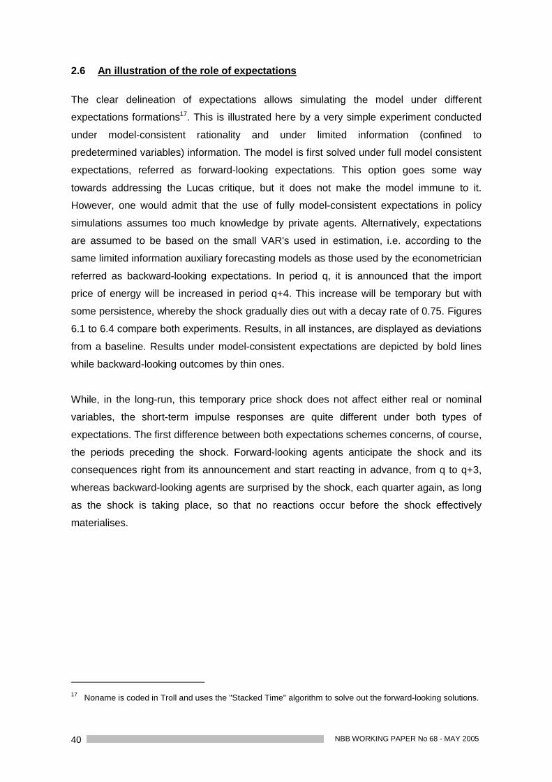
NBB WORKING PAPER No 68 - MAY 200540
2.6 An illustration of the role of expectations
The clear delineation of expectations allows simulating the model under different
expectations formations17. This is illustrated here by a very simple experiment conducted
under model-consistent rationality and under limited information (confined to
predetermined variables) information. The model is first solved under full model consistent
expectations, referred as forward-looking expectations. This option goes some way
towards addressing the Lucas critique, but it does not make the model immune to it.
However, one would admit that the use of fully model-consistent expectations in policy
simulations assumes too much knowledge by private agents. Alternatively, expectations
are assumed to be based on the small VAR's used in estimation, i.e. according to the
same limited information auxiliary forecasting models as those used by the econometrician
referred as backward-looking expectations. In period q, it is announced that the import
price of energy will be increased in period q+4. This increase will be temporary but with
some persistence, whereby the shock gradually dies out with a decay rate of 0.75. Figures
6.1 to 6.4 compare both experiments. Results, in all instances, are displayed as deviations
from a baseline. Results under model-consistent expectations are depicted by bold lines
while backward-looking outcomes by thin ones.
While, in the long-run, this temporary price shock does not affect either real or nominal
variables, the short-term impulse responses are quite different under both types of
expectations. The first difference between both expectations schemes concerns, of course,
the periods preceding the shock. Forward-looking agents anticipate the shock and its
consequences right from its announcement and start reacting in advance, from q to q+3,
whereas backward-looking agents are surprised by the shock, each quarter again, as long
as the shock is taking place, so that no reactions occur before the shock effectively
materialises.
17 Noname is coded in Troll and uses the "Stacked Time" algorithm to solve out the forward-looking solutions.
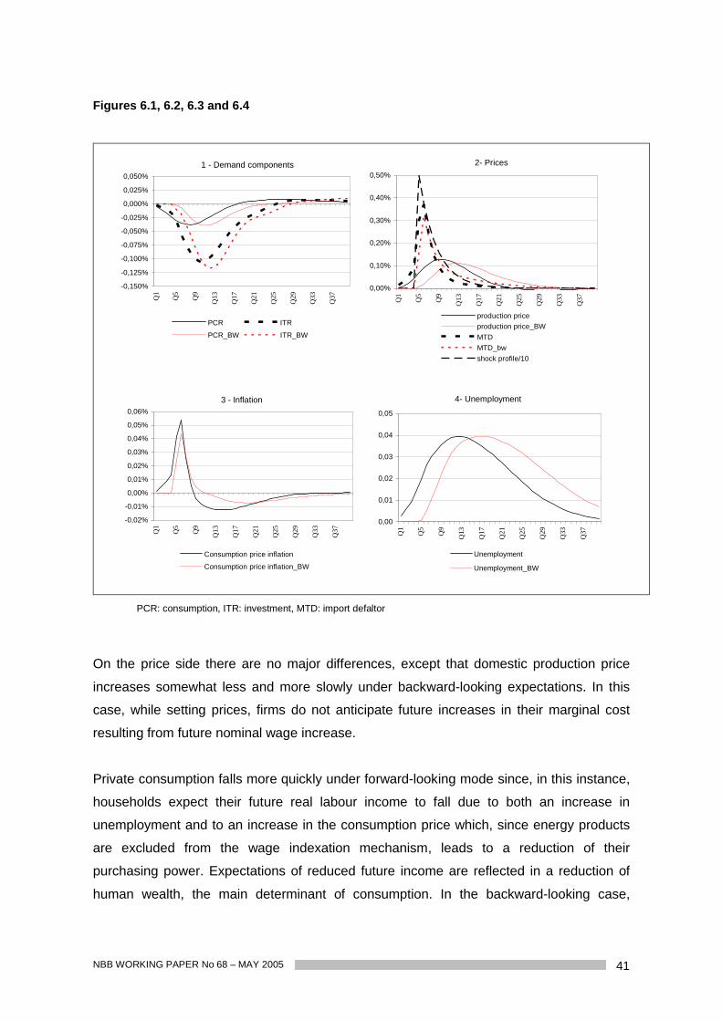
NBB WORKING PAPER No 68 – MAY 2005 41
Figures 6.1, 6.2, 6.3 and 6.4
1 - Demand components
-0,150%
-0,125%
-0,100%
-0,075%
-0,050%
-0,025%
0,000%
0,025%
0,050%
Q1
Q5
Q9
Q13
Q17
Q21
Q25
Q29
Q33
Q37
PCR ITR
PCR_BW ITR_BW
2- Prices
0,00%
0,10%
0,20%
0,30%
0,40%
0,50%
Q1
Q5
Q9
Q13
Q17
Q21
Q25
Q29
Q33
Q37
production priceproduction price_BWMTDMTD_bwshock profile/10
3 - Inflation
-0,02%
-0,01%
0,00%
0,01%
0,02%
0,03%
0,04%
0,05%
0,06%
Q1
Q5
Q9
Q13
Q17
Q21
Q25
Q29
Q33
Q37
Consumption price inflation
Consumption price inflation_BW
4- Unemployment
0,00
0,01
0,02
0,03
0,04
0,05
Q1
Q5
Q9
Q13
Q17
Q21
Q25
Q29
Q33
Q37
Unemployment
Unemployment_BW
PCR: consumption, ITR: investment, MTD: import defaltor
On the price side there are no major differences, except that domestic production price
increases somewhat less and more slowly under backward-looking expectations. In this
case, while setting prices, firms do not anticipate future increases in their marginal cost
resulting from future nominal wage increase.
Private consumption falls more quickly under forward-looking mode since, in this instance,
households expect their future real labour income to fall due to both an increase in
unemployment and to an increase in the consumption price which, since energy products
are excluded from the wage indexation mechanism, leads to a reduction of their
purchasing power. Expectations of reduced future income are reflected in a reduction of
human wealth, the main determinant of consumption. In the backward-looking case,

NBB WORKING PAPER No 68 - MAY 200542
human wealth only decreases gradually as households observe the reduction in their
current income (they fail to recognise immediately the size and the persistence of this
reduction) so that, in this framework, aggregate consumption decreases mainly as a
consequence of the reduction in employment. Investment decreases more quickly under
forward-looking expectations since the future contractions of output are taken into account
and thereafter it recovers somewhat more rapidly in expectation of the subsequent
recovery of output.
Figure 6.4 highlights the sluggishness in the response of unemployment which returns to
base more slowly than output. This is, in some way, the mirror image of the long lead and
lag found in the employment equation.
3. DIAGNOSTIC SIMULATIONS
3.1 Preliminary remarks
In the model, exchange rates and the short term interest rate are treated exogenously.
Endogenisation of these variables would require an analysis of output, price and interest
rate determination at the eurozone level. When such an analysis is necessary, we can use
a DSGE model for the euroarea, such as Smets and Wouters (2003). Therefore, all the
simulations presented in this paper are conditional on the assumption of constant short
and long term nominal interest rates. The purpose of the following simulations is to
investigate model properties. They are not intended to provide a comprehensive account
of the model's multipliers. All the diagnostic simulations presented have been run for a
period of 25 years18. The choice for such a long simulation period is dictated by two
requirements. First, solving models under model-consistent expectations requires a
terminal date sufficiently far into the future to avoid the simulation results to be affected by
the choice of the terminal date. Second, simulating the model over a long period allows an
inspection of the long run solution of the model. Each benchmark simulation exercise has
been performed with the fiscal rule switched off over the entire period. Simulation results
are reported relative to a base constructed over the future which is residual-free. This
means that no add-factors are added and. the baseline scenario is not calibrated to match
observed data in the first quarters. As such, the base does not represent a projection in the
usual meaning of the word.
18 However for readability reasons, the charts hereafter only show the first 10 years.

NBB WORKING PAPER No 68 – MAY 2005 43
The model has been estimated on an equation by equation basis. As already mentioned,
for Polynomial Adjustment Costs equations, this approach gives the flexibility to introduce
various types of expectation formation and in that way offers an easy alternative to the
model-consistent expectations scheme. A system estimation would however provide
probability distributions for the parameters and allow us to generate probability
distributions for simulated values of the variables. Such a system estimation would be
difficult if not unfeasible with the size of our model. Since we cannot get this full
characterisation of parameter uncertainty, we have conducted simple numerical
experiments to explore whether the magnitudes of some relevant parameters are
important for the ultimate effect of the shocks. Tables 4-a to 4-d in appendix A1
investigate how the results discussed in the next sub-sections are dependent on our
benchmark parameterisation. It separately examines the repercussions on the simulations
outcomes of:
- an increase in the elasticity of consumption w.r.t. financial wealth from 5 p.c. to 10 p.c.
to the detriment of human wealth;
- variations of 20 p.c. in the price elasticity so that the domestic and export price
elasticities vary from 4 to 6;
- variations in the dynamic coefficient of the short term impact of changes in employment
on consumption from 0.25 to 0.619;
- variations of coefficient of the cash-flow in the short term investment equation from 0.2
to 0.55;
- the introduction of the fiscal rule from the beginning of the fifth year after the shock
onwards;
the remaining parameters being left unchanged.
This sensitivity analysis demonstrates that the results that follow are not too over-sensitive
to these perturbations. However, the range of the distribution of the medium and long-run
impact of consumption is large for the foreign demand shock. In this case, the distribution
is skewed towards the minimum: the maximum effect is far above the average one
because these permanent shocks have clear positive (i.e. downwards) effects on the
public debt. When experiments are conducted with a fiscal rule, these positive effects are
redistributed in the form of lump-sum transfers to households. These transfers increase
their disposable income and, since the shock is permanent, they also increase their human
wealth, being private consumption's main determinant.
19 When this coefficient is set at 0.6, the model does not converge in the case of the labour supply shock.

NBB WORKING PAPER No 68 - MAY 200544
3.2 A foreign demand shock
This shock is characterized by a 1 p.c. permanent expansion of Belgian real export
markets, both at the extra and intra euro-area levels. It has been imposed that this
increase in foreign demand leaves prices inside and outside the eurozone unaffected. In
response, Belgian exports increase by almost 1 p.c. which raises GDP by around 0.4 p.c.
The improvement in the trade balance is limited through the large import content of
exported goods. The major domestic change concerns investment which positively reacts
to output as well as to improved profitability. After five years consumption increases in line
with the increase in human wealth. However, in the short run, during the job creation
period, consumption overshoots its long run level. The reduction of unemployment allows
wages to increase, which puts upwards pressure on marginal costs as well as on prices.
As nominal rates are fixed and inflation increases somewhat ex-post, the real interest rates
decline. This also contributes to sustain consumption and investment. Note that this
increase in domestic prices and the associated deterioration in competitiveness is
responsible for the fact that exports grow less than export markets in the medium term.

NBB WORKING PAPER No 68 – MAY 2005 45
Figures 7a, 7b, 7c and 7d
Foreign demand shock : Employment
0,00%0,10%0,20%0,30%0,40%0,50%0,60%0,70%0,80%0,90%1,00%
Employment
Foreign demand shock: GDP components
0,00%
0,20%
0,40%
0,60%
0,80%
1,00%
1,20%
GDP PCRITR XTRM TR
Foreign demand shock: Prices and costs
0,00%
0,05%
0,10%
0,15%
0,20%
0,25%
XTD M TDhome good price M arginal costPCD
Foreign demand shock : Inflation
-0,005%
0,000%
0,005%
0,010%
0,015%
0,020%
Consumpt ion price inf lat ion
wage inf lat ion
PCR: consumption, ITR: investment, XTR: exports, MTR: imports, XTD: export deflator,MTD: import deflator
3.3 An indirect tax shock
The average VAT rate is permanently increased by 1ppt. The transmission from changes
in VAT rates to consumer prices is not immediate. Indeed, many prices are labelled VAT
included and there may be menu costs to changing them. Besides, even if it is true for
individual prices labelled exclusive VAT that a 1 ppt. increase in VAT rate should lead on
impact to a 1 p.c. increase in the selling prices, at the aggregate macro level, it may not be
the case. Since such measures are generally announced well in advance and are subject
to legislative lags, consumers may bring their expenditures plans forward (in case of a VAT
increase) or delay them (in case of a decrease). In the real world, there is a variety of VAT

NBB WORKING PAPER No 68 - MAY 200546
rates and, most of the time changes to them have not been applied uniformly but rather
differently to individual rates. Consequently, shocks to some rates may not lead to an
immediate one-for-one impact on the consumption deflator because their weights change.
For all these reasons, transmission lags are difficult to estimate empirically and there is
uncertainty surrounding them. Therefore, we have fixed them as a 3-quarter distributive lag
with coefficients 0.5, 0.3, 0.2.
Figures 8a, 8b, 8c and 8d
Indirect Tax shock :GDP components
-1,60%-1,40%-1,20%
-1,00%-0,80%-0,60%-0,40%
-0,20%0,00%0,20%
GDP PCR
ITR XTRM TR
Indirect Tax shock: Prices and costs
0,00%
0,50%
1,00%
1,50%
2,00%
2,50%
XTD M TDhome good price M arginal costPCD
Indirect Tax shock : Inflation
-0,10%
0,00%
0,10%
0,20%
0,30%
0,40%
0,50%
0,60%
Consumpt ion price inflat ion
wage inf lat ion
Indirect Tax shock: Employment
-1,20%
-1,00%
-0,80%
-0,60%
-0,40%
-0,20%
0,00%
Employment
PCR: consumption, ITR: investment, XTR: exports, MTR: imports, XTD: export deflator,MTD: import deflator
This being said, such a measure widens the gap between output price "at factors cost" and
the private consumption deflator "at market price". Given the lag structure, the latter
increases on impact by 0.5 p.c. and, after 3 quarters, the pass-through is complete while
the former has only changed by 0.3 p.c. within this time horizon. Thereafter, as wages are
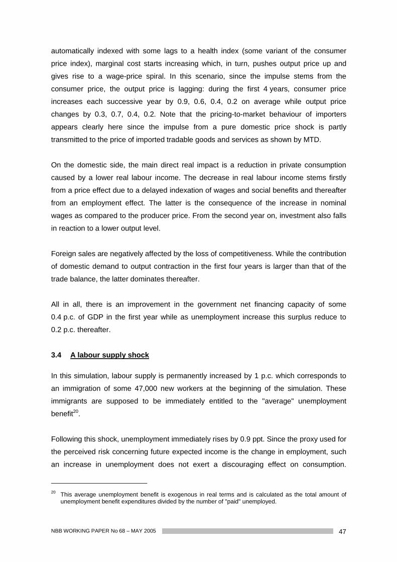
NBB WORKING PAPER No 68 – MAY 2005 47
automatically indexed with some lags to a health index (some variant of the consumer
price index), marginal cost starts increasing which, in turn, pushes output price up and
gives rise to a wage-price spiral. In this scenario, since the impulse stems from the
consumer price, the output price is lagging: during the first 4 years, consumer price
increases each successive year by 0.9, 0.6, 0.4, 0.2 on average while output price
changes by 0.3, 0.7, 0.4, 0.2. Note that the pricing-to-market behaviour of importers
appears clearly here since the impulse from a pure domestic price shock is partly
transmitted to the price of imported tradable goods and services as shown by MTD.
On the domestic side, the main direct real impact is a reduction in private consumption
caused by a lower real labour income. The decrease in real labour income stems firstly
from a price effect due to a delayed indexation of wages and social benefits and thereafter
from an employment effect. The latter is the consequence of the increase in nominal
wages as compared to the producer price. From the second year on, investment also falls
in reaction to a lower output level.
Foreign sales are negatively affected by the loss of competitiveness. While the contribution
of domestic demand to output contraction in the first four years is larger than that of the
trade balance, the latter dominates thereafter.
All in all, there is an improvement in the government net financing capacity of some
0.4 p.c. of GDP in the first year while as unemployment increase this surplus reduce to
0.2 p.c. thereafter.
3.4 A labour supply shock
In this simulation, labour supply is permanently increased by 1 p.c. which corresponds to
an immigration of some 47,000 new workers at the beginning of the simulation. These
immigrants are supposed to be immediately entitled to the "average" unemployment
benefit20.
Following this shock, unemployment immediately rises by 0.9 ppt. Since the proxy used for
the perceived risk concerning future expected income is the change in employment, such
an increase in unemployment does not exert a discouraging effect on consumption.
20 This average unemployment benefit is exogenous in real terms and is calculated as the total amount ofunemployment benefit expenditures divided by the number of "paid" unemployed.

NBB WORKING PAPER No 68 - MAY 200548
Moreover disposable income mechanically increases by the amount of the transfer from
the government to the new unemployment benefit recipients. This boosts aggregate
consumption which, in turn, stimulates output and investment. Such an increase in
domestic absorption leads to a deterioration of the trade balance even when
competitiveness gains in both the import and the export markets show up. The increase in
employment resulting from a higher output and a lower real "producer" wage falls short of
the initial jump in labour supply. This stems from the lack of sufficient flexibility in wage
formation which prevents wages from falling enough to absorb effectively the whole
increase in labour supply. As a result, the unemployment rate rises permanently by some
0.6 p.c. This result is somewhat higher than that reported by Karanassou, Sala and
Snower (2004) who obtain an increase of 0.42 p.c. for an average of 11 EU countries
(including Belgium). Finally, government net financing capacity deteriorates by 0.2 p.c. of
GDP.

NBB WORKING PAPER No 68 – MAY 2005 49
Figures 9a, 9b, 9c and 9d
Labour supply shock : GDP components
0,00%
0,10%
0,20%
0,30%
0,40%
0,50%
0,60%
0,70%
GDP PCRITR XTRM TR
Labour supply shock: Prices and costs
-0,50%-0,45%-0,40%-0,35%-0,30%-0,25%-0,20%-0,15%-0,10%-0,05%0,00%
XTD M TDhome good price M arginal costPCD
Labour supply shock : Inflation
-0,20%
-0,15%
-0,10%
-0,05%
0,00%
0,05%
Consumpt ion price inf lation
wage inf lat ion
Labour supply shock: Employment
0,00%
0,20%
0,40%
0,60%
0,80%
1,00%
Employment
PCR: consumption, ITR: investment, XTR: exports, MTR: imports, XTD: export deflator,MTD: import deflator
3.5 An oil price shock
In this exercise, we analyse the effect of a permanent 10 p.c. increase in the price of
crude oil expressed in euro.
Following this price shock, there is a quick and sustained increase in import prices which
rise by almost 0.8%. Since imported items enter the private consumption directly also, its
deflator also increases by around 0.25% in year one. Higher import prices also push up
intermediate goods producers' price, initiating a cost-price spiral. As a result the
consumption deflator increases by 0.9% in the long-run. The shock also affects export
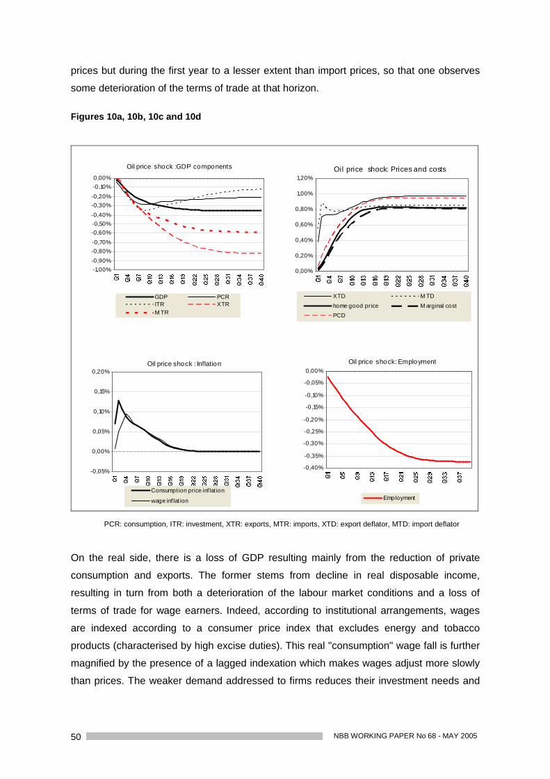
NBB WORKING PAPER No 68 - MAY 200550
prices but during the first year to a lesser extent than import prices, so that one observes
some deterioration of the terms of trade at that horizon.
Figures 10a, 10b, 10c and 10d
Oil price shock :GDP components
-1,00%-0,90%-0,80%-0,70%-0,60%-0,50%-0,40%-0,30%-0,20%-0,10%0,00%
GDP PCRITR XTRM TR
Oil price shock : Inflation
-0,05%
0,00%
0,05%
0,10%
0,15%
0,20%
Consumption price inf lat ion
wage inf lat ion
Oil price shock: Prices and costs
0,00%
0,20%
0,40%
0,60%
0,80%
1,00%
1,20%
XTD M TDhome good price M arginal costPCD
Oil price shock: Employment
-0,40%
-0,35%
-0,30%
-0,25%
-0,20%
-0,15%
-0,10%
-0,05%
0,00%
Employment
PCR: consumption, ITR: investment, XTR: exports, MTR: imports, XTD: export deflator, MTD: import deflator
On the real side, there is a loss of GDP resulting mainly from the reduction of private
consumption and exports. The former stems from decline in real disposable income,
resulting in turn from both a deterioration of the labour market conditions and a loss of
terms of trade for wage earners. Indeed, according to institutional arrangements, wages
are indexed according to a consumer price index that excludes energy and tobacco
products (characterised by high excise duties). This real "consumption" wage fall is further
magnified by the presence of a lagged indexation which makes wages adjust more slowly
than prices. The weaker demand addressed to firms reduces their investment needs and

NBB WORKING PAPER No 68 – MAY 2005 51
the effect the price of energy exerts on costs in the building industry, combined with the
decrease in households' real disposable income, causes a fall in housing investment. After
three years, investment recovers somewhat in so far that firms are now able to improve
their financing capacities. As time passes wage inflation catches up with consumer price
and employment stops deteriorating, allowing consumption to stabilise, be it still below
base. The main driving force behind the reduction in real output in the long run is the drop
in exports following a loss of external competitiveness. Note that in reality such an oil price
shock is likely to increase also competitors' prices reducing thereby the effect on
competitiveness.
4. CONCLUDING REMARKS
In this paper, we depicted the core structure of the small open economy quarterly model of
the National Bank of Belgium.
The goal was to build a model that is able to provide quantitative input into the policy
analysis and projection processes with a framework that has explicit micro-foundations and
expectations. Since a model as Noname obeys economic theory not only in the long-term
but, for many variables, also in the dynamic adjustment process, its responses are easier
to understand from an economic point of view than those of traditional backward-looking
models with arbitrarily added unrestricted polynomials in the lag operator that nicely fit the
data. We also believe that it is therefore more suited in the context of a coherent analysis
of responses by rational agents reacting to news about future events than was the case in
traditional econometric models. Another element of the strategy involves the decision to
maintain the model relatively compact to keep the structure simple enough for projections
and simulation purposes.
Some key differences between our chosen setup and that typically found in the literature
have been focused on:
- Noname can be operated under different assumptions concerning expectation formation
and whatever the option used it converges to the same long-run solution;
- In order to rationalise the introduction of dynamics, the intertemporal optimisation
problem of households and firms is subjected to costs related to the adjustment of
decision variables. Noname, as FRB/US, makes use of a richer dynamic specification
than the quadratic cost function encountered in former testing of the rational

NBB WORKING PAPER No 68 - MAY 200552
expectations hypothesis. Such richer dynamics are introduced by means of Polynomial
Adjustment Costs (PAC);
- We have pricing-to-market and hence flexible mark-ups and incomplete pass-through
even in equilibrium thanks to "translog" preferences rather than the usual and easier to
work with "CES" aggregator which generates incomplete pass-through only along the
transition path;
- A CES production function characterises the data better than the previous Cobb-
Douglas production function, and it generates a below one elasticity of substitution
between capital and labour;
- In case the model is utilised with endogenous wages, we use a simplified version of the
time-dependent pricing framework à la Dootsey, King and Wollman which is able to
generate hump-shaped responses contrary to the Calvo model used in most DSGE
models or to an error correction model used in more traditional settings, which implies
the largest response to a shock during the period the shock occurs.
Most of the equations taken individually have acceptable statistical properties although it
was not our first goal to exactly match the data. The reason for not sticking to the data
individually was that a model is more interesting taken as a whole and single equation and
partial equilibrium analysis have hardly some value-added in this context. In addition, as
Kapetanios et al. (2005) have noted in a paper on policy-oriented modelling (p.3)
"Replicating the data is rarely the objective. There are many reasons for this. Data is often
subject to substantial revisions for long periods of time, so one may be replicating a
chimera; it can also be influenced by many special factors that are hard to specify, ...".
Finally, diagnostic simulations suggest that the impulse responses of the model to
exogenous shocks are reasonable.

NBB WORKING PAPER No 68 – MAY 2005 53
References
Acemoglu D. (2000), Labor- and capital- augmenting technical change, NBER, WP 7544.
Barten A.P. and Ph. Jeanfils (2004), "The evaluation of dynamic properties of large empiricalmacroeconomic models", in S. Késenne and C.Reyns., (eds), Liber Amicorum Prof. Dr.Robert Van Straelen, Garant, Antwerpen, Apeldoorn, 88-94.
Basu S. (1996), "Procyclical productivity: increasing returns of cyclical utilisation?", QuarterlyJournal of Economics, 111, 719-751.
Basu S. and M. Kimball (1997), Cyclical productivity with unobserved input variation, NBERWorking Paper 5915.
Bénassy J.-P. (2001), "Output and inflation persistence under price and wage staggering: analyticalresults", mimeo, November.
Bergin P. (2003), "A model of relative national price levels under pricing to market", EuropeanEconomic Review, 47, 569-586.
Bergin P. and R. Feenstra (2001), "Pricing-to-market, staggered contracts, and real exchange ratepersistence", Journal of International Economics, 54, 333-359.
Bergin P. and R. Feenstra (2000), "Staggered price setting, translog preferences, and endogenouspersistence", Journal of Monetary Economics, 45, 657-680.
Black R., D. Laxton, D. Rose and R. Tetlow (1994), The Bank of Canada’s new quarterly projectionmodel: SSQPM, Bank of Canada , Technical Report n° 72.
Blanchard O.J. (1985), "Debt, Deficit, and Finite Horizons", Journal of Political Economy, 93, 223-247.
Blanchard O.J and S. Fischer (1989), Lectures on macroeconomics, The MIT Press.
Brayton F., E. Mauskopf, D. Reifschneider, P. Tinsley and J. Williams (1997), "The role ofexpectations in the FRB/US macroeconomic model", Federal Reserve Bulletin, 83 (4), 227-245.
Brayton F., A. Levin, R. Tryon and J. Williams (1997), "The evolution of macro models at theFederal Reserve Board", Carnegie-Rochester Conference Series on Public Policy 47, 43-81.
Calvo G. (1983), "Staggered prices in a utility-maximizing environment", Journal of MonetaryEconomics, 12, 983-998.
Campbell J.Y. and N.G. Mankiw (1989), "Consumption, income, and interest rates: reinterpretingthe time series evidence", in NBER Macroeconomics Annual, 1989.

NBB WORKING PAPER No 68 - MAY 200554
Corsetti G. and L. Dedola (2002), Macroeconomics of international price discrimination, ECBworking paper 176, September.
Dolado J., J.W. Galbraith and A. Banerjee (1991), "Estimating intertemporal quadratic adjustmentcosts models with integrated series", International Economic Review, 32 (4), 919-936.
Dombrecht M. and Ph. Moës (1998), "Inflation and unemployment in an open economy", Economicand Financial Modelling, 5(2), 53-94.
Dotsey M., R.G. King and A.L. Wolman (1999), "State-dependant pricing and general equilibriumdynamics of money and output", Quarterly Journal of Economics, 114, 655-690.
Duffy J. and C. Papageorgiou (2000), "A cross-country empirical investigation of the aggregateproduction function specification", Journal of Economic Growth, 5, March, 87-120.
Eugène B., Ph. Jeanfils and B. Robert (2003), La consommation en Belgique, NBB Working Paper,Document Series 39, June.
Freystätter H. (2003), Price setting behavior in an open economy and the determination of Finnishforeign trade price, Bank of Finland Studies E:25.
Gali J. (1995), Non-Walrasian unemployment fluctuations, NBER working paper 5337, November.
Jeanfils Ph. (2000), A model with explicit expectations for Belgium, NBB Working Paper, ResearchSeries 4, March.
Kapetanios G., A. Pagan and A. Scott (2005), Making a match: combining theory and evidence inpolicy-oriented macroeconomic modelling, mimeo, January 2005.
Karanassou, M., S. Sala and D.J. Snower (2004), Unemployment in the European Union:institutions, prices and growth, CESifo Working Paper 1247, July.
Klump R. and H. Preissler (2000), "CES production function and economic growth", ScandinavianJournal of Economics, 102 (1), pp 41-56.
Kosicki S. and P. Tinsley (2002), Alternative sources of the lag dynamics of inflation, FederalReserve of Kansas City, RWP 02-12.
Kosicki S. and P. Tinsley (2001), Dynamic specifications in optimizing trend-deviation macromodels, Federal Reserve of Kansas City, RWP 01-03.
Kosicki S. and P. Tinsley (1999), "Vector rational error correction", Journal of Economic Dynamicsand Control, 23, 1299-1327.
Layard R., S.J. Nickell and R. Jackman (1991). Unemployment: Macroeconomic Performance andthe Labour Market, Oxford University Press.
Lucas R. (1976), "Econometric policy evaluation: a critique". In The Phillips curve and the labourmarket, Carnegie-Rochester Conference Series on Public Policy 1, 19-46.
NBB WORKING PAPER No 68 – MAY 2005 55
McHugh J. (2002), Wage centralization, union bargaining, and macroeconomic performance, IMFworking paper 02143, August.
Murchinson S., A. Renisson and Z. Zhu (2004), A structural small open-economy model forCanada, Bank of Canada, Working Paper 2004-4, February.
Monacelli T. (2003), Monetary policy in a low pass-through environment, ECB working paper 227,April.
Nickell S. (1985), "Error correction, partial adjustment and all that: an expository note", OxfordBulletin of Economics and Statistics, 47 (2), 119-129.
Ripatti A. and J. Vilmunen (2001), Declining labour share - evidence of a change in the underlyingproduction technology, Bank of Finland, Discussion Papers 10/2001.
Rowthorn R.E. (1999), "Unemployment, wage bargaining and capital-labour substitution"Cambridge, Journal of Economics, 23 (4), 413-425.
Smets F. and R. Wouters (2003), "An estimated dynamic stochastic general equilibrium model ofthe euro area" Journal of the European Economic Association,1 (September), 1123-1175.
Taylor J.B. (1980), "Aggregate dynamics and staggered contracts", Journal of Political Economy,88, 1-24.
Tinsley P.A. (1993), "Fitting both data and theories: polynomial adjustment costs and errorcorrection decision rules", Finance and Economics Discussions Series, 93-21, FederalReserve Board, Washington, D.C.
Tinsley P.A. (2002), "Rational error correction", Computational economics, 19 (2), April, 197-225.
Trigari A. (2003), Labour market search, wage bargaining and inflation dynamics, mimeo, August.
von zur Muelhen P. (2001), "The effect of past and future economic fundamentals on spending andpricing behaviour in the FRB/US macroeconomic model", Finance and EconomicsDiscussions Series, 2001-12, Federal Reserve Board, Washington, D.C.
Willman A. (2002), Euro Area production function and potential output: a supply side systemapproach, ECB Working paper 153, June.
Zanetti F. (2003), Non-Walrasian labor market and the European Business cycle, mimeo BostonCollege, April.

NBB WORKING PAPER No 68 - MAY 200556
Appendix A1: Impact of model parameters on simulation results
Table 4a - Sensitivity of the results from a foreign demand shock to perturbationsin selected parameters
YER benchmark max min avg NetX benchmark max min avg
q=1 0.30% 0.30% 0.29% 0.30% q=1 0.28% 0.28% 0.27% 0.28%q=5 0.36% 0.40% 0.35% 0.37% q=5 0.23% 0.24% 0.19% 0.22%q=9 0.39% 0.45% 0.38% 0.40% q=9 0.21% 0.22% 0.16% 0.20%q=21 0.34% 0.43% 0.33% 0.35% q=21 0.21% 0.22% 0.13% 0.20%q=inf 0.30% 0.32% 0.28% 0.30% q=inf 0.19% 0.20% 0.14% 0.19%
PCR benchmark max min avg PCD benchmark max min avg
q=1 0.02% 0.04% 0.02% 0.03% q=1 0.00% 0.00% 0.00% 0.00%q=5 0.16% 0.26% 0.13% 0.18% q=5 0.01% 0.01% 0.01% 0.01%q=9 0.19% 0.33% 0.15% 0.20% q=9 0.04% 0.04% 0.03% 0.04%q=21 0.09% 0.31% 0.08% 0.11% q=21 0.11% 0.13% 0.10% 0.11%q=inf 0.06% 0.16% 0.05% 0.07% q=inf 0.12% 0.14% 0.11% 0.12%
ITR benchmark max min avg ULC benchmark max min avg
q=1 0.14% 0.15% 0.14% 0.14% q=1 -0.22% -0.22% -0.22% -0.22%q=5 0.40% 0.45% 0.36% 0.40% q=5 -0.11% -0.10% -0.11% -0.11%q=9 0.54% 0.63% 0.48% 0.55% q=9 -0.01% -0.01% -0.02% -0.01%q=21 0.51% 0.65% 0.44% 0.53% q=21 0.16% 0.19% 0.14% 0.17%q=inf 0.44% 0.49% 0.38% 0.44% q=inf 0.18% 0.21% 0.16% 0.18%
Table 4b - Sensitivity of the results from a indirect tax shock to perturbationsin selected parameters
YER benchmark max min avg NetX benchmark max min avg
q=1 0.02% 0.02% 0.02% 0.02% q=1 0.07% 0.07% 0.07% 0.07%q=5 -0.29% -0.27% -0.31% -0.29% q=5 0.03% 0.05% 0.01% 0.03%q=9 -0.52% -0.49% -0.55% -0.52% q=9 -0.11% -0.08% -0.13% -0.11%q=21 -0.81% -0.76% -0.87% -0.81% q=21 -0.55% -0.52% -0.57% -0.55%q=inf -0.83% -0.78% -0.87% -0.83% q=inf -0.67% -0.64% -0.69% -0.66%
PCR benchmark max min avg PCD benchmark max min avg
q=1 -0.07% -0.06% -0.08% -0.07% q=1 0.52% 0.52% 0.52% 0.52%q=5 -0.45% -0.40% -0.51% -0.45% q=5 1.34% 1.34% 1.33% 1.34%q=9 -0.57% -0.50% -0.65% -0.57% q=9 1.78% 1.79% 1.77% 1.78%q=21 -0.46% -0.39% -0.54% -0.46% q=21 2.20% 2.25% 2.16% 2.20%q=inf -0.38% -0.36% -0.44% -0.39% q=inf 2.18% 2.25% 2.12% 2.18%
ITR benchmark max min avg ULC benchmark max min avg
q=1 0.00% 0.00% -0.01% 0.00% q=1 -0.04% -0.04% -0.05% -0.04%q=5 -0.28% -0.26% -0.32% -0.28% q=5 1.12% 1.13% 1.11% 1.12%q=9 -0.50% -0.45% -0.56% -0.50% q=9 1.52% 1.55% 1.50% 1.52%q=21 -0.41% -0.27% -0.52% -0.40% q=21 1.87% 1.94% 1.80% 1.87%q=inf -0.21% -0.05% -0.35% -0.21% q=inf 1.75% 1.86% 1.66% 1.75%
Notes : the table compares the maximum and minimum as well as the average effects of the shock when the size of someparameters varies as compared to our benchmark parameterisation on GDP, YER, on private consumption, PCR, on gross fixedcapital formation, ITR, on net exports, NetX, on private consumption deflator, PCD and on unit labour costs, ULC.
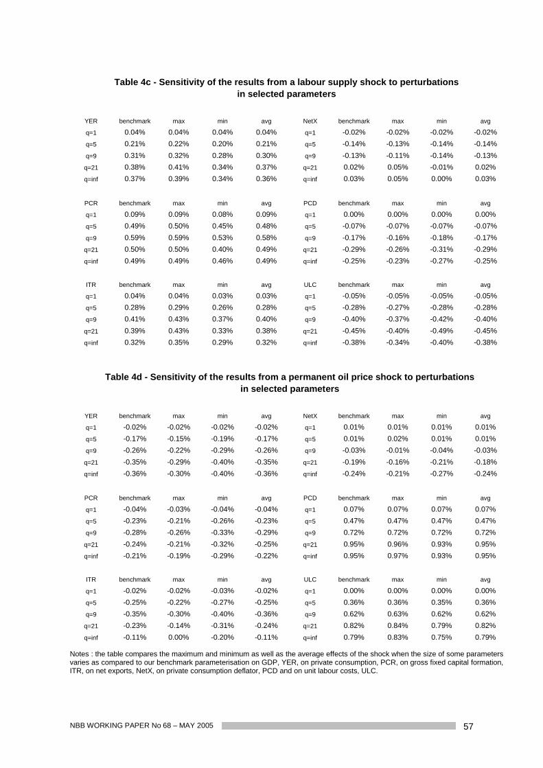
NBB WORKING PAPER No 68 – MAY 2005 57
Table 4c - Sensitivity of the results from a labour supply shock to perturbationsin selected parameters
YER benchmark max min avg NetX benchmark max min avg
q=1 0.04% 0.04% 0.04% 0.04% q=1 -0.02% -0.02% -0.02% -0.02%q=5 0.21% 0.22% 0.20% 0.21% q=5 -0.14% -0.13% -0.14% -0.14%q=9 0.31% 0.32% 0.28% 0.30% q=9 -0.13% -0.11% -0.14% -0.13%q=21 0.38% 0.41% 0.34% 0.37% q=21 0.02% 0.05% -0.01% 0.02%q=inf 0.37% 0.39% 0.34% 0.36% q=inf 0.03% 0.05% 0.00% 0.03%
PCR benchmark max min avg PCD benchmark max min avg
q=1 0.09% 0.09% 0.08% 0.09% q=1 0.00% 0.00% 0.00% 0.00%q=5 0.49% 0.50% 0.45% 0.48% q=5 -0.07% -0.07% -0.07% -0.07%q=9 0.59% 0.59% 0.53% 0.58% q=9 -0.17% -0.16% -0.18% -0.17%q=21 0.50% 0.50% 0.40% 0.49% q=21 -0.29% -0.26% -0.31% -0.29%q=inf 0.49% 0.49% 0.46% 0.49% q=inf -0.25% -0.23% -0.27% -0.25%
ITR benchmark max min avg ULC benchmark max min avg
q=1 0.04% 0.04% 0.03% 0.03% q=1 -0.05% -0.05% -0.05% -0.05%q=5 0.28% 0.29% 0.26% 0.28% q=5 -0.28% -0.27% -0.28% -0.28%q=9 0.41% 0.43% 0.37% 0.40% q=9 -0.40% -0.37% -0.42% -0.40%q=21 0.39% 0.43% 0.33% 0.38% q=21 -0.45% -0.40% -0.49% -0.45%q=inf 0.32% 0.35% 0.29% 0.32% q=inf -0.38% -0.34% -0.40% -0.38%
Table 4d - Sensitivity of the results from a permanent oil price shock to perturbationsin selected parameters
YER benchmark max min avg NetX benchmark max min avg
q=1 -0.02% -0.02% -0.02% -0.02% q=1 0.01% 0.01% 0.01% 0.01%q=5 -0.17% -0.15% -0.19% -0.17% q=5 0.01% 0.02% 0.01% 0.01%q=9 -0.26% -0.22% -0.29% -0.26% q=9 -0.03% -0.01% -0.04% -0.03%q=21 -0.35% -0.29% -0.40% -0.35% q=21 -0.19% -0.16% -0.21% -0.18%q=inf -0.36% -0.30% -0.40% -0.36% q=inf -0.24% -0.21% -0.27% -0.24%
PCR benchmark max min avg PCD benchmark max min avg
q=1 -0.04% -0.03% -0.04% -0.04% q=1 0.07% 0.07% 0.07% 0.07%q=5 -0.23% -0.21% -0.26% -0.23% q=5 0.47% 0.47% 0.47% 0.47%q=9 -0.28% -0.26% -0.33% -0.29% q=9 0.72% 0.72% 0.72% 0.72%q=21 -0.24% -0.21% -0.32% -0.25% q=21 0.95% 0.96% 0.93% 0.95%q=inf -0.21% -0.19% -0.29% -0.22% q=inf 0.95% 0.97% 0.93% 0.95%
ITR benchmark max min avg ULC benchmark max min avg
q=1 -0.02% -0.02% -0.03% -0.02% q=1 0.00% 0.00% 0.00% 0.00%q=5 -0.25% -0.22% -0.27% -0.25% q=5 0.36% 0.36% 0.35% 0.36%q=9 -0.35% -0.30% -0.40% -0.36% q=9 0.62% 0.63% 0.62% 0.62%q=21 -0.23% -0.14% -0.31% -0.24% q=21 0.82% 0.84% 0.79% 0.82%q=inf -0.11% 0.00% -0.20% -0.11% q=inf 0.79% 0.83% 0.75% 0.79%
Notes : the table compares the maximum and minimum as well as the average effects of the shock when the size of some parametersvaries as compared to our benchmark parameterisation on GDP, YER, on private consumption, PCR, on gross fixed capital formation,ITR, on net exports, NetX, on private consumption deflator, PCD and on unit labour costs, ULC.

NBB WORKING PAPER No 68 - MAY 200558
Appendix A2: Main dynamic behavioural equations
1. PRICE AND WAGE EQUATIONS IN THE MODEL
1.1. Prices(i) Main driving domestic price
The price of the domestic intermediate goods, Hp , is the main driving domestic price variable in themodel.
The target or optimal price for domestic intermediate goods is given by:
ttHt* mtd23.0ucc,wc77.0p
whereucc,wc t is unit cost of production with "w" being the hourly wage cost and the user cost of
capital being defined as rppErIucc 1t,CDtOD with rp designing a constant riskpremium arbitrarily fixed at 0.025.
This shows that firms set their price not only in response to changes in their own costs but also inresponse to the prices set by their competitors. The relative weight depends on the share of non-traded goods which determines the proportion of their competitors that are foreign.
The dynamic equation for domestic intermediate goods is :
1yy0.001)p(Eleads355.0
plags676.0)p(p0.12p
ss1-t
iHt1-t
1-Ht11Ht1-HtHt
R²: 0.34; dw: 2.64; LM(4): 24.6 (0.0); JB: 1.61 (0.44); Arch(4): 6.16(0.18)where y is the growth rate of private output and ssy its steady-state value.
(ii) Consumption deflator
Since final goods result from the combination of domestic products and imported goods, priceindices for consumption (PCD), and also for investment by companies and exported goods areweighted functions of the price set by domestic suppliers ( Hp ) and the price of imported goods
(mtd). Given that Hp is defined at factor costs, the consumption deflator is modelled by addingindirect tax rates. In addition the energy price is added to account for the direct price effect on fuel.
Thus consumption price inflation evolves according to:
ttHt
2t2t1t1ttt
pei013.0mtd307.0p68.04.0)tipcd(15.0)tipcd(45.0tipcd
[ mean lag (inflation): 1.9 ]
where the import price of energy, PEI, and the indirect tax rate, ti, are exogenous and the rate ofgrowth of the price of imports, MTD, is given by
1yy0.001)mtd(Eleads91.0)mtd(mtd0.34mtd ss
1-tiHt1-t1t1-tt
R²: 0.51; dw: 2.03; LM(4): 4.65 (0.32); JB: 0.16 (0.92); Arch(4): 3.58(0.46)and the target level is

NBB WORKING PAPER No 68 – MAY 2005 59
HttFt*t p27.0pei06.0p67.0mtd
And finally, the price that serves in the indexation mechanism of wages and transfers evolvesaccording to:
tttt pmazout008.0pei013.0pcd005025.12pcdwhere pmazout stands for heating oil which is not excluded from the health index.
(iii) Exports and GDP deflatorsThe rate of growth of the price of exports, XTD, is given by
)xtd(Eleads76.0xtd0.15)xtd(xtd0.24xtd it1-t1-t1t1-tt
R²: 0.59; dw: 1.79; LM(4): 12.1 (0.02); JB: 0.28 (0.86); Arch(4): 0.41(0.98)where the target level is
*Ftttt
*t p25.0pei046.0ucc,wc624.0xtd
The GDP deflator is defined by an accounting identity that divides the value of GDP, YEN, by itsvolume, YER:
YERYENYED
and it has no feedback on other prices.
1.2. Wages
Note that fuel, tobacco and alcohol are excluded from the basket used to calculate the "health"consumption price index, PCD2. Therefore, for forecasts, the wage rate excluding indexation(wrh_R) is assumed to be exogenous and the endogenous nominal wage is obtained by indexing itaccording to:
)2PCD*12/32PCD*12/82PCD*12/1(*R_wrhwrh 2t1tttt
However if necessary for simulations, an endogenous "real" wage may be used. This is a "flexible"version of (1.67) :
t
ttttt,L
Ct u1
k1log1ulogb2.018.01log05.0logw
and after indexation the aggregate wage index is calculated as in (2.12)
2. DEMAND COMPONENTS
2.1. Consumption
Due to habit formation consumption does not immediately adjust to changes in the desired level. Inaddition to taking into account these delayed adjustments, the dynamic consumption equation alsodepends on changes in employment to capture uncertainty in future income:
3
0iitit1-t1-t21t1-tt 4Lln*0.42)c(Eleads485.0clags538.0)c(c0.178c
R²: 0.39; dw: 1.83; LM(4): 6.72 (0.15); JB: 0.04(0.98); Arch(4): 3.64(0.45)where *c is given in (1.19)
2.2. Housing investment
The equilibrium ratio of housing investment to consumption is a function of the relative price ofconsumption to the cost of new houses and on a mortgage interest rate.

NBB WORKING PAPER No 68 - MAY 200560
ttt1tttt*t pcdihxn4.0rkrhpcdErmt2.1cihr
)ihr(Eleads396.0ihrlags604.0)ihr(ihr0.19ihr it1-t1-t31t1-tt
R²: 0.74; dw:1.75; LM(4): 4.46 (0.34); JB: 0.26 (0.87); Arch(4): 3.97(0.41);sample restricted to 1990:1 to 2003:4
2.3. Business investment
4
1i1t1titi-t
it1-t1-t3L2t1-tt
IODKREOTNNON0.39
)kre(Eleads65.0iorlags21.0)ngln-kre(ior0.12ior
R²: 0.42; dw: 2.54; LM(4): 12.2 (0.02); JB: 2.5 (0.28); Arch(4): 4.4(0.35)
2.4. Exports
1t*
1ftt*ftt
2t1tt*
1t1tt
xtdp4.0xtdp6.03.0ex_wdr32.0in_wdr07.0in_wdr23.0in_wdr7.068.0xtrxtr15.0xtr
R²: 0.34; dw: 1.57; LM(4): 2.96 (0.56); JB: 3.26 (0.19); Arch(4): 3.46 (0.48)
where xtr* is given by combining (1.32) and (1.33).
2.5. Imports
1t*t
*1t1tt duc49.0mtr79.0mtrmtr40.0mtr
R²: 0.54; dw: 2.26; LM(4): 10.5 (0.03); JB: 1.82 (0.40); Arch(4): 25.7 (0.00)
where mtr* is given by (1.56).
3. EMPLOYMENT
)hourslpn(Eleads79.0
y16.0)hourslpnhourslpn(16.0hourslpn
itit1-t
t1t1-t1t1-ttt
R²: 0.61; dw: 1.97; LM(4): 6.21 (0.18); JB: 3.64 (0.16); Arch(4): 4.80 (0.30)
where the optimal level comes from log-linearisation of (1.28a) :
)t003845.0(48.0pwrh52.052.0yhourslpn Htttttt
and hours per employee evolve according to :
1t1tt
1t1t1t1t1tt
hours17.0krey13.0krey17.0etpl1.0durconhours38.0hours
R²: 0.43; dw: 2.25; LM(4): 6.61 (0.15); JB: 0.66 (0.71); Arch(4): 4.65 (0.32)
where durcon is conventional working time and etpl reflects the proportion full-time workers.

NBB WORKING PAPER No 68 – MAY 2005 61
NATIONAL BANK OF BELGIUM - WORKING PAPERS SERIES
1. "Model-based inflation forecasts and monetary policy rules" by M. Dombrecht and R. Wouters,Research Series, February 2000.
2. "The use of robust estimators as measures of core inflation" by L. Aucremanne, ResearchSeries, February 2000.
3. "Performances économiques des Etats-Unis dans les années nonante" by A. Nyssens,P. Butzen, P. Bisciari, Document Series, March 2000.
4. "A model with explicit expectations for Belgium" by P. Jeanfils, Research Series, March 2000.
5. "Growth in an open economy: some recent developments" by S. Turnovsky, Research Series,May 2000.
6. "Knowledge, technology and economic growth: an OECD perspective" by I. Visco,A. Bassanini, S. Scarpetta, Research Series, May 2000.
7. "Fiscal policy and growth in the context of European integration" by P. Masson, ResearchSeries, May 2000.
8. "Economic growth and the labour market: Europe's challenge" by C. Wyplosz, ResearchSeries, May 2000.
9. "The role of the exchange rate in economic growth: a euro-zone perspective" byR. MacDonald, Research Series, May 2000.
10. "Monetary union and economic growth" by J. Vickers, Research Series, May 2000.
11. "Politique monétaire et prix des actifs: le cas des Etats-Unis" by Q. Wibaut, Document Series,August 2000.
12. "The Belgian industrial confidence indicator: leading indicator of economic activity in the euroarea?" by J.J. Vanhaelen, L. Dresse, J. De Mulder, Document Series, November 2000.
13. "Le financement des entreprises par capital-risque" by C. Rigo, Document Series, February2001.
14. "La nouvelle économie" by P. Bisciari, Document Series, March 2001.
15. "De kostprijs van bankkredieten" by A. Bruggeman and R. Wouters, Document Series,April 2001.
16. "A guided tour of the world of rational expectations models and optimal policies" byPh. Jeanfils, Research Series, May 2001.
17. "Attractive Prices and Euro - Rounding effects on inflation" by L. Aucremanne and D. Cornille,Documents Series, November 2001.
18. "The interest rate and credit channels in Belgium: an investigation with micro-level firm data" byP. Butzen, C. Fuss and Ph. Vermeulen, Research series, December 2001.
19 "Openness, imperfect exchange rate pass-through and monetary policy" by F. Smets andR. Wouters, Research series, March 2002.
20. "Inflation, relative prices and nominal rigidities" by L. Aucremanne, G. Brys, M. Hubert,P. J. Rousseeuw and A. Struyf, Research series, April 2002.
21. "Lifting the burden: fundamental tax reform and economic growth" by D. Jorgenson, Researchseries, May 2002.

NBB WORKING PAPER No 68 - MAY 200562
22. "What do we know about investment under uncertainty?" by L. Trigeorgis, Research series,May 2002.
23. "Investment, uncertainty and irreversibility: evidence from Belgian accounting data" byD. Cassimon, P.-J. Engelen, H. Meersman, M. Van Wouwe, Research series, May 2002.
24. "The impact of uncertainty on investment plans" by P. Butzen, C. Fuss, Ph. Vermeulen,Research series, May 2002.
25. "Investment, protection, ownership, and the cost of capital" by Ch. P. Himmelberg,R. G. Hubbard, I. Love, Research series, May 2002.
26. "Finance, uncertainty and investment: assessing the gains and losses of a generalised non-linear structural approach using Belgian panel data", by M. Gérard, F. Verschueren, Researchseries, May 2002.
27. "Capital structure, firm liquidity and growth" by R. Anderson, Research series, May 2002.
28. "Structural modelling of investment and financial constraints: where do we stand?" byJ.- B. Chatelain, Research series, May 2002.
29. "Financing and investment interdependencies in unquoted Belgian companies: the role ofventure capital" by S. Manigart, K. Baeyens, I. Verschueren, Research series, May 2002.
30. "Development path and capital structure of Belgian biotechnology firms" by V. Bastin,A. Corhay, G. Hübner, P.-A. Michel, Research series, May 2002.
31. "Governance as a source of managerial discipline" by J. Franks, Research series, May 2002.
32. "Financing constraints, fixed capital and R&D investment decisions of Belgian firms" byM. Cincera, Research series, May 2002.
33. "Investment, R&D and liquidity constraints: a corporate governance approach to the Belgianevidence" by P. Van Cayseele, Research series, May 2002.
34. "On the Origins of the Franco-German EMU Controversies" by I. Maes, Research series,July 2002.
35. "An estimated dynamic stochastic general equilibrium model of the Euro Area", by F. Smetsand R. Wouters, Research series, October 2002.
36. "The labour market and fiscal impact of labour tax reductions: The case of reduction ofemployers' social security contributions under a wage norm regime with automatic priceindexing of wages", by K. Burggraeve and Ph. Du Caju, Research series, March 2003.
37. "Scope of asymmetries in the Euro Area", by S. Ide and Ph. Moës, Document series,March 2003.
38. "De autonijverheid in België: Het belang van het toeleveringsnetwerk rond de assemblage vanpersonenauto's", by F. Coppens and G. van Gastel, Document series, June 2003.
39. "La consommation privée en Belgique", by B. Eugène, Ph. Jeanfils and B. Robert, Documentseries, June 2003.
40. "The process of European monetary integration: a comparison of the Belgian and Italianapproaches", by I. Maes and L. Quaglia, Research series, August 2003.
41. "Stock market valuation in the United States", by P. Bisciari, A. Durré and A. Nyssens,Document series, November 2003.

NBB WORKING PAPER No 68 – MAY 2005 63
42. "Modeling the Term Structure of Interest Rates: Where Do We Stand?, by K. Maes, Researchseries, February 2004.
43. Interbank Exposures: An Empirical Examination of System Risk in the Belgian BankingSystem, by H. Degryse and G. Nguyen, Research series, March 2004.
44. "How Frequently do Prices change? Evidence Based on the Micro Data Underlying the BelgianCPI", by L. Aucremanne and E. Dhyne, Research series, April 2004.
45. "Firms' investment decisions in response to demand and price uncertainty", by C. Fuss andPh. Vermeulen, Research series, April 2004.
46. "SMEs and Bank Lending Relationships: the Impact of Mergers", by H. Degryse,N. Masschelein and J. Mitchell, Research series, May 2004.
47. "The Determinants of Pass-Through of Market Conditions to Bank Retail Interest Rates inBelgium", by F. De Graeve, O. De Jonghe and R. Vander Vennet, Research series, May 2004.
48. "Sectoral vs. country diversification benefits and downside risk", by M. Emiris, Research series,May 2004.
49. "How does liquidity react to stress periods in a limit order market?", by H. Beltran, A. Durré andP. Giot, Research series, May 2004.
50. "Financial consolidation and liquidity: prudential regulation and/or competition policy?", byP. Van Cayseele, Research series, May 2004.
51. "Basel II and Operational Risk: Implications for risk measurement and management in thefinancial sector", by A. Chapelle, Y. Crama, G. Hübner and J.-P. Peters, Research series,May 2004.
52. "The Efficiency and Stability of Banks and Markets", by F. Allen, Research series, May 2004.
53. "Does Financial Liberalization Spur Growth?" by G. Bekaert, C.R. Harvey and C. Lundblad,Research series, May 2004.
54. "Regulating Financial Conglomerates", by X. Freixas, G. Lóránth, A.D. Morrison and H.S. Shin,Research series, May 2004.
55. "Liquidity and Financial Market Stability", by M. O'Hara, Research series, May 2004.
56. "Economisch belang van de Vlaamse zeehavens: verslag 2002", by F. Lagneaux, Documentseries, June 2004.
57. "Determinants of Euro Term Structure of Credit Spreads", by A. Van Landschoot, Researchseries, July 2004.
58. "Macroeconomic and Monetary Policy-Making at the European Commission, from the RomeTreaties to the Hague Summit", by I. Maes, Research series, July 2004.
59. "Liberalisation of Network Industries: Is Electricity an Exception to the Rule?", by F. Coppensand D. Vivet, Document series, September 2004.
60. "Forecasting with a Bayesian DSGE model: an application to the euro area", by F. Smets andR. Wouters, Research series, September 2004.
61. "Comparing shocks and frictions in US and Euro Area Business Cycle: a Bayesian DSGEapproach", by F. Smets and R. Wouters, Research series, October 2004.
62. "Voting on Pensions: A Survey", by G. de Walque, Research series, October 2004.

NBB WORKING PAPER No 68 - MAY 200564
63. "Asymmetric growth and inflation developments in the acceding countries: a new assessment",by S. Ide and Ph. Moës, Research series, November 2004.
64. "Importance économique du Port Autonome de Liège: rapport 2002", by F. Langeaux,Document series, November 2004.
65. "Price-setting behaviour in Belgium: what can be learned from an ad hoc survey", byL. Aucremanne and M. Druant, Research series, March 2005.
66. "Time-dependent versus State-dependent Pricing: A Panel Data Approach to the Determinantsof Belgian Consumer Price Changes", by L. Aucremanne and E. Dhyne, Research series, April2005.
67. "Indirect effects – A formal definition and degrees of dependency as an alternative to technicalcoefficients", by F. Coppens, Research series, May 2005.
68. "Noname – A new quarterly model for Belgium", by Ph. Jeanfils and K. Burggraeve, Researchseries, May 2005.