Working Paper No. 616 February 2019
34
Optimal development of electricity generation mix considering fossil fuel phase-out and strategic multi-area interconnection Desta Z. Fitiwi ab* , Muireann Lynch ab , Valentin Bertsch c Abstract: Increased renewable generation worldwide is posing new challenges for power system planners. The location, as well as the level and operation, of each generation resource is increasingly important. This work presents a constrained Generation Expansion Planning (GEP) optimization model. One of the salient features of the model is its reasonably accurate representation of the physical characteristics of power systems. It considers both active and reactive power flows in a linear manner. Natural voltage magnitude deviations from nominal values across the transmission system are also captured in the resulting model. Therefore, the network model employed here closely resembles the AC optimal power flow one. We apply the model to a realistic test system of the island of Ireland and determine the optimal generation expansion and operation out to 2030 under a range of demand and policy scenarios. Our results show that costs and emissions are driven primarily by the decommissioning of old inefficient generation units. High renewable targets, on the other hand, render increased carbon prices relatively ineffective in reducing system emissions. *Corresponding Author: [email protected] Keywords: Generation expansion planning, optimal generation mix, RES integration, strategic interconnection, carbon leakage. Acknowledgements: Desta Z. Fitiwi acknowledges support by a research grant from the Science Foundation Ireland (SFI) under the SFI Strategic Partnership Programme Grant number SFI/15/SPP/E3125. The opinions, findings and conclusions or recommendations expressed in this material are those of the authors and do not necessarily reflect the views of the Science Foundation. This work has also benefited from the valuable support of EirGrid, the Transmission System Operator in the Republic of Ireland. Hence, the authors would like to greatly acknowledge EirGrid’s contributions in providing data and insights for this work. a. Economic and Social Research Institute, Dublin b. Department of Economics, Trinity College Dublin c. German Aerospace Center (DLR), Germany ESRI working papers represent un-refereed work-in-progress by researchers who are solely responsible for the content and any views expressed therein. Any comments on these papers will be welcome and should be sent to the author(s) by email. Papers may be downloaded for personal use only. Working Paper No. 616 February 2019
Transcript of Working Paper No. 616 February 2019

Optimal development of electricity generation mix considering fossil fuel phase-out and strategic multi-area interconnection
Desta Z. Fitiwiab*, Muireann Lynchab, Valentin Bertschc
Abstract: Increased renewable generation worldwide is posing new challenges for power system planners. The location, as well as the level and operation, of each generation resource is increasingly important. This work presents a constrained Generation Expansion Planning (GEP) optimization model. One of the salient features of the model is its reasonably accurate representation of the physical characteristics of power systems. It considers both active and reactive power flows in a linear manner. Natural voltage magnitude deviations from nominal values across the transmission system are also captured in the resulting model. Therefore, the network model employed here closely resembles the AC optimal power flow one.
We apply the model to a realistic test system of the island of Ireland and determine the optimal generation expansion and operation out to 2030 under a range of demand and policy scenarios. Our results show that costs and emissions are driven primarily by the decommissioning of old inefficient generation units. High renewable targets, on the other hand, render increased carbon prices relatively ineffective in reducing system emissions.
*Corresponding Author: [email protected]
Keywords: Generation expansion planning, optimal generation mix, RES integration, strategic interconnection, carbon leakage.
Acknowledgements: Desta Z. Fitiwi acknowledges support by a research grant from the Science Foundation Ireland (SFI) under the SFI Strategic Partnership Programme Grant number SFI/15/SPP/E3125. The opinions, findings and conclusions or recommendations expressed in this material are those of the authors and do not necessarily reflect the views of the Science Foundation. This work has also benefited from the valuable support of EirGrid, the Transmission System Operator in the Republic of Ireland. Hence, the authors would like to greatly acknowledge EirGrid’s contributions in providing data and insights for this work.
a. Economic and Social Research Institute, Dublinb. Department of Economics, Trinity College Dublinc. German Aerospace Center (DLR), Germany
ESRI working papers represent un-refereed work-in-progress by researchers who are solely responsible for the content and any views expressed therein. Any comments on these papers will be welcome and should be sent to the author(s) by email. Papers may be downloaded for personal use only.
Working Paper No. 616
February 2019

2
1. Introduction
1.1. Background Concerns over climate change have led to new and sustained efforts to decarbonise energy systems [1], [2], which in the case of the electricity sector require an expansion in renewable generation technologies. This expansion has implications for generation expansion planning (GEP) exercises, which determine the optimal development of power production mixes over medium- to long-term time horizons. In particular, GEP methodologies simultaneously determine the optimal sizes, locations and generation schedules of power production technologies in a least-cost manner. The variability in the supply of various sources of renewable generation, such as wind and solar power, and the spatial distribution of same, pose new challenges for GEP.
The literature on GEP is wide and extensive, spanning over several decades. References [3], [4], [5] and [6] present extensive reviews of the existing literature on GEP and related aspects. Authors in [7] highlight the importance of a flexible power system, and investigate ways of improving operational flexibility within a GEP framework with the aim of meeting renewable and emission reduction targets. The GEP problem can be considered independently [8] or in tandem with other objectives such as transmission expansion planning (TEP) [9]–[15]. Furthermore, GEP methodologies are often employed to determine the impact of a new technology and/or system development. Examples include carbon capture and storage [16], energy storage systems [17], renewable integration [18], [19], power-to-gas [20], demand response [14], electric vehicles [21] and [22] and distributed generation [21].
The GEP problem can be formulated in a static planning framework in which decisions are made for a target year (e.g. [12], [15], [23] and [24]) or a dynamic framework as in [25], [26]–[28]. The work in [10] initially formulates the GEP and TEP optimization problems in a static and multi-level planning framework, but with the capability of performing year-by-year dynamic analysis. Sequential static planning or a rolling horizon approach is adopted when the planning horizon is long [13]. Strict differentiation between dynamic and static planning is not possible as they are not clearly defined in the literature.
Power systems contain various sources of uncertainty on both the supply and demand sides [29], and the limited predictability of renewable generation increases this uncertainty. Authors in [30] incorporate uncertainty from renewable power sources by selecting representative days for their input data set. The work in [12] accounts for uncertainty in wind power generation using a Monte Carlo Simulation (MCS) approach in a composite generation and transmission expansion planning (GTEP) framework. Some studies have also included reliability issues in a GEP framework, for example [9], which considers generator and transmission line outages in a GTEP optimization. Authors in [13] perform an in-depth stochastic GTEP exercise with uncertainties in demand, fuel prices, costs of greenhouse gas emissions and supply disruptions.
In this paper, we develop a network-constrained GEP optimization framework that considers short- and long-term uncertainties. Short-term uncertainty (also known as operational uncertainty) arises from variable power production sources (such as wind and solar), electricity demand and forced outages of conventional generators. We model the uncertainty by considering a sufficiently large number of operational situations. Sources of long-term uncertainty include demand composition and growth, carbon and fuel prices, and policy interventions, including
3
RES-E penetration and decarbonisation targets, system-non synchronous penetration (SNSP) limit, phasing out fossil fuel based power generation, and regional or cross-country interconnections.
The optimisation model developed in this paper is based on a linearised AC optimal power flow (LinAC-OPF). Unlike the commonly used DC-OPF network model, LinAC-OPF linearly represents both active and reactive power flows and considers natural voltage magnitude differences across nodes.
1.2. Contribution of this paper The original contributions of this paper are threefold. First, this paper represents a significant methodological improvement through its consideration of the transmission system. Many GEP models ignore the transmission system entirely and essentially model the entire network as one node. These models are incapable of considering the spatial aspects of GEP, which as discussed are of increasing importance as we nowadays witness a paradigm shift in the manner electricity is being sourced. There is a growing trend in the production of electricity using distributed energy resources (renewables, in particular), gradually making the often conventional and centralised way of power generation obsolete. Moreover, distributed renewables generation development may be more economically viable alternative given the spatially distributed nature of such resources.
In particular, generation expansion decisions obtained without considering transmission constraints may prove infeasible from an operational standpoint, or they may require massive investments in grid infrastructures. In the extant literature, GEP models are mostly formulated without taking account of transmission network effects [7], [8], [16], [19], [20], [23]–[26], [28], [29], [31]–[36]. A few papers model transmission networks as pipelines [17], [21], [37]. In some cases, GEP models include transmission considerations using a lossless Direct Current Optimal Power Flow [9]–[11], [14], [15]. They thus implicitly assume a uniform voltage across the system, and cannot take account of reactive power flow constraints. This paper addresses this gap in the literature by introducing a linearised AC-OPF into a GEP framework.
Secondly, this work utilises a test system represented by a detailed and unique dataset. Unlike many of the papers referenced above which consider relatively small test systems, this paper models the entire synchronous system of the island of Ireland. GEP in Ireland is understudied in the literature, with [26], which performs an optimal renewable allocation, being the only example. The Irish system is a particularly interesting test system: it is one synchronous island system comprising two weakly interconnected control areas (North and South) with limited (DC) interconnection to other systems which renders the balancing of electricity supply and demand in real time particularly challenging. Ireland has a significant wind resource, which has led to large-scale investment in wind generation, with a policy-driven target of 40% of total generation to be met by renewable electricity by 2020. These high levels of renewable generation have in turn led to high levels of simultaneous non-synchronous penetration (up to 75%). Furthermore, the wind resource is located primarily on the west coast, with the largest load centres located on the east coast, and so the transmission system significantly impacts the optimal location and operation of generation facilities. The Irish system also has limited storage facilities; the variability of renewable generation must thus be accommodated by other generation units.
The third main contribution of this work emanates from the policy scenarios considered in our analysis. These scenarios are demand-driven, infrastructure-driven and policy-driven, and so

4
the results are instructive for policy makers and system operators alike. The implications of high-level decisions can be seen at each node of the transmission system. Demand growth projections are provided by EirGrid, the transmission system operator (TSO) in Ireland. These demand projections, along with projections regarding future infrastructure and policy outcomes on issues such as e-heating and e-mobility, form four different scenarios. Sensitivities are also performed around parameters such as carbon prices and renewable expansion.
The remainder of this paper is structured as follows. A description of the model and solution approach is provided in Section 2. Section 3 presents relevant information regarding data and assumptions made during the analysis. Section 4 presents numerical results obtained from the case study. Some discussions and insights from the results are also contained in this section. Section 5 presents sensitivity analysis, and section 6 concludes.
2. Problem Formulation
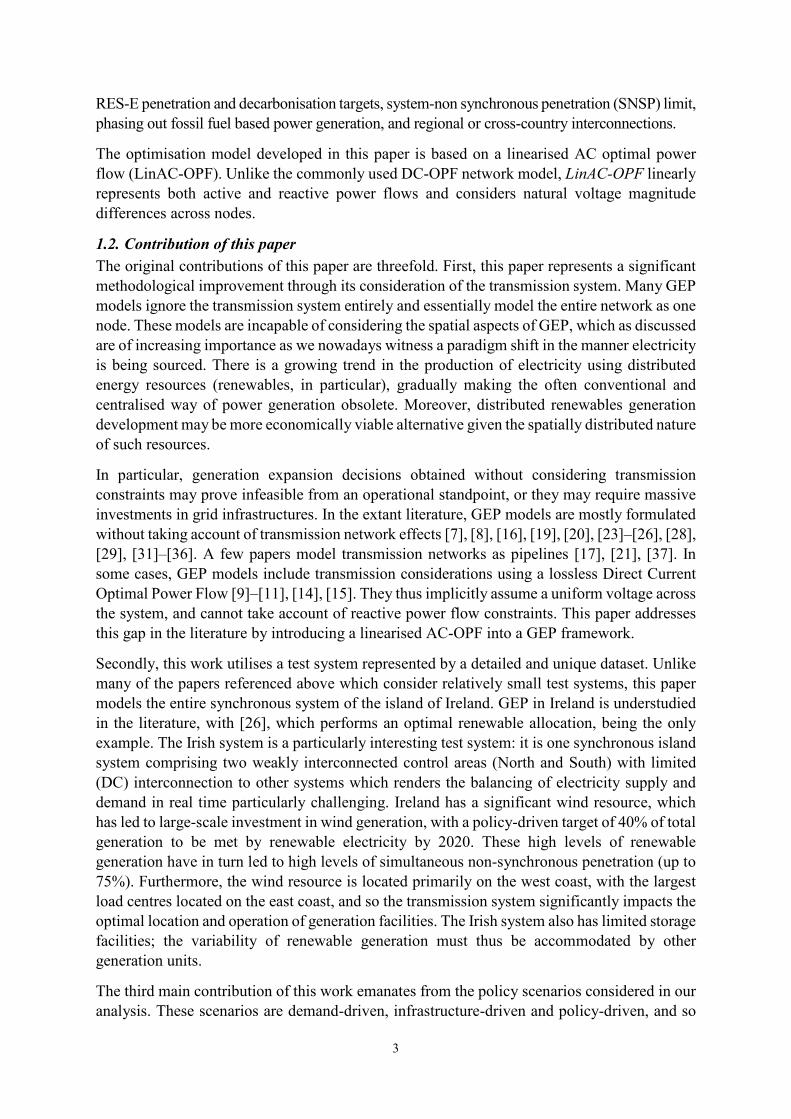
2.1. Modeling Approach and Associated Terminologies This modelling approach considers n potential future scenarios, each with a specific probability, which represent a realisation of the relevant sources of long-term uncertainty such as demand growth, carbon prices and fuel prices. The demand growth projections are primarily driven by different potential growth rates of datacentres in Ireland, as projected by the System Operator, EirGrid [38]. The scenarios themselves are a collection of “snapshots”, or hourly realisations of demand and renewable energy availability. The snapshots are chosen to form a realistic representation of each scenario (see section 2.3). The GEP problem itself is formulated as a multi-stage problem, i.e. the planning horizon is divided into multiple decision periods. The GEP model solves for optimal values of all control variables at each decision period, considering all potential future scenarios and the probability of same. Thus the model generates one solution which is optimal for the probability-weighted combination of all scenarios. The multi-stage and multi-scenario GEP modelling framework, and the expansion solution structure, is illustrated in Figure 1.
2.2. Algebraic Formulation This work develops an optimization model suitable for medium and long-term power generation expansion planning. The GEP problem is formulated as a constrained optimisation with overall cost minimisation as an objective function, and several techno-economic constraints that must be satisfied.
2.2.1 Objective Function The objective function of system-wide costs consists of several terms, shown in (1). The entire problem is formulated as a multi-stage stochastic linear programming model. GEP problems generally involve integer decision variables due to the lumpy increments of generation capacity investment. However, for the case studies in this paper, these variables are relaxed to continuous ones in order to enhance problem tractability, leading to an LP model. The objective function in (1) is the sum of the Net Present Value (NPV) of five cost terms.
𝑀𝑀𝑀𝑀𝑀𝑀𝑀𝑀𝑀𝑀𝑀𝑀𝑀𝑀𝑀𝑀 𝑇𝑇𝑇𝑇 = 𝑇𝑇𝑇𝑇𝑀𝑀𝑇𝑇𝑇𝑇 + 𝑇𝑇𝑀𝑀𝑇𝑇 + 𝑇𝑇𝑇𝑇𝑇𝑇 + 𝑇𝑇𝑇𝑇𝑇𝑇𝑇𝑇𝑇𝑇 + 𝑇𝑇𝑇𝑇𝑀𝑀𝑀𝑀𝑇𝑇 (1)
𝑇𝑇𝑇𝑇𝑀𝑀𝑇𝑇𝑇𝑇 represents the NPV of total investment costs in new generation capacity:
5
Figure 1. Illustration modelling approach and associated terminologies
𝑇𝑇𝑇𝑇𝑀𝑀𝑇𝑇𝑇𝑇 = �(1 + 𝑟𝑟)−𝑡𝑡𝑇𝑇𝑀𝑀𝑇𝑇𝑇𝑇𝑡𝑡𝑔𝑔𝑔𝑔𝑔𝑔
𝑡𝑡𝑡𝑡Ω𝑡𝑡���������������𝑁𝑁𝑁𝑁𝑁𝑁 𝑜𝑜𝑜𝑜 𝑖𝑖𝑔𝑔𝑖𝑖𝑔𝑔𝑖𝑖𝑡𝑡𝑖𝑖𝑔𝑔𝑔𝑔𝑡𝑡 𝑐𝑐𝑜𝑜𝑖𝑖𝑡𝑡
(2)
where
𝑇𝑇𝑀𝑀𝑇𝑇𝑇𝑇𝑡𝑡𝑔𝑔𝑔𝑔𝑔𝑔 = � �
𝑟𝑟(1 + 𝑟𝑟)𝐿𝐿𝐿𝐿𝑔𝑔
(1 + 𝑟𝑟)𝐿𝐿𝐿𝐿𝑔𝑔 − 1𝑇𝑇𝑇𝑇𝑔𝑔,𝑖𝑖(𝑥𝑥𝑔𝑔,𝑖𝑖,𝑡𝑡 − 𝑥𝑥𝑔𝑔,𝑖𝑖,𝑡𝑡−1)
𝑖𝑖𝑡𝑡𝛺𝛺𝑖𝑖𝑔𝑔𝑡𝑡𝛺𝛺𝑔𝑔 ; 𝑥𝑥𝑔𝑔,𝑖𝑖,0 = 0 (3)
𝑇𝑇𝑇𝑇𝑔𝑔,𝑖𝑖 represents the investment cost of generators; 𝑥𝑥𝑔𝑔,𝑖𝑖,𝑡𝑡 is the investment variable of generator g. 𝐿𝐿𝑇𝑇𝑔𝑔 is the life time of generator g. All investment costs are weighted by the capital recovery
factor, 𝑟𝑟(1+𝑟𝑟)𝐿𝐿𝑇𝑇𝑔𝑔
(1+𝑟𝑟)𝐿𝐿𝑇𝑇𝑔𝑔−1. The formulation in (3) ensures the cost of each component is considered
only once in the summation.
The second term (𝑇𝑇𝑀𝑀𝑇𝑇) in (1) denotes the NPV of total maintenance costs, which is the sum of the maintenance costs of new and existing generators and of network components:
Solution Structure Stochastic Solutions
Problem Structure Scenarios
Planning stages
Snapshots
Rea
lizat
ions
6
𝑇𝑇𝑀𝑀𝑇𝑇 = �(1 + 𝑟𝑟)−𝑡𝑡
𝑡𝑡𝑡𝑡Ω𝑡𝑡 �𝑀𝑀𝑀𝑀𝑀𝑀𝑇𝑇𝑡𝑡
𝑔𝑔𝑔𝑔𝑔𝑔 + 𝑀𝑀𝑀𝑀𝑀𝑀𝑇𝑇𝑡𝑡𝑔𝑔𝑡𝑡𝑛𝑛��������������������������
𝑁𝑁𝑁𝑁𝑁𝑁 𝑜𝑜𝑜𝑜 𝑖𝑖𝑚𝑚𝑖𝑖𝑔𝑔𝑡𝑡𝑔𝑔𝑔𝑔𝑚𝑚𝑔𝑔𝑐𝑐𝑔𝑔 𝑐𝑐𝑜𝑜𝑖𝑖𝑡𝑡𝑖𝑖
(4)
where 𝑀𝑀𝑀𝑀𝑀𝑀𝑇𝑇𝑡𝑡𝑔𝑔𝑔𝑔𝑔𝑔 is the maintenance costs of new and existing generators at each time stage:
𝑀𝑀𝑀𝑀𝑀𝑀𝑇𝑇𝑡𝑡𝑔𝑔𝑔𝑔𝑔𝑔 = � �𝑀𝑀𝑇𝑇𝑔𝑔𝑁𝑁
𝑖𝑖𝑡𝑡𝛺𝛺𝑖𝑖𝑔𝑔𝑡𝑡𝛺𝛺𝑔𝑔𝑥𝑥𝑔𝑔,𝑖𝑖,𝑡𝑡 + � �𝑀𝑀𝑇𝑇𝑔𝑔𝐸𝐸
𝑖𝑖𝑡𝑡𝛺𝛺𝑖𝑖𝑔𝑔𝑡𝑡𝛺𝛺𝑔𝑔𝑢𝑢𝑔𝑔,𝑖𝑖,𝑡𝑡 (5)
and 𝑀𝑀𝑀𝑀𝑀𝑀𝑇𝑇𝑡𝑡𝑔𝑔𝑡𝑡𝑛𝑛 is the maintenance cost of an existing line. This cost is included only when its corresponding utilisation variable is different from zero:
𝑀𝑀𝑀𝑀𝑀𝑀𝑇𝑇𝑡𝑡𝑔𝑔𝑡𝑡𝑛𝑛 = � 𝑀𝑀𝑇𝑇𝑛𝑛𝐸𝐸
𝑛𝑛𝑡𝑡𝛺𝛺𝑒𝑒ℓ𝑢𝑢𝑛𝑛,𝑡𝑡 + � 𝑀𝑀𝑇𝑇𝑡𝑡𝑟𝑟𝐸𝐸
𝑡𝑡𝑟𝑟𝑡𝑡𝛺𝛺𝐸𝐸𝑡𝑡𝑡𝑡
𝑢𝑢𝑡𝑡𝑟𝑟,𝑖𝑖,𝑡𝑡 (6)
The third term 𝑇𝑇𝑇𝑇𝑇𝑇 in (1) refers to the total cost of energy in the system from both new and existing generators:
where
𝑇𝑇𝑇𝑇𝑡𝑡𝑔𝑔𝑔𝑔𝑔𝑔 = � 𝜌𝜌𝑖𝑖 � 𝜋𝜋𝑤𝑤 � �(𝜆𝜆𝑔𝑔,𝑖𝑖,𝑤𝑤,𝑡𝑡
𝑁𝑁𝑁𝑁 𝑃𝑃𝑔𝑔,𝑖𝑖,𝑖𝑖,𝑤𝑤,𝑡𝑡𝑁𝑁
𝑖𝑖𝑡𝑡𝛺𝛺𝑖𝑖𝑔𝑔𝑡𝑡𝛺𝛺𝑔𝑔+ 𝜆𝜆𝑔𝑔,𝑖𝑖,𝑤𝑤,𝑡𝑡
𝐸𝐸
𝑤𝑤𝑡𝑡𝛺𝛺𝑤𝑤𝑃𝑃𝑔𝑔,𝑖𝑖,𝑖𝑖,𝑤𝑤,𝑡𝑡𝐸𝐸 )
𝑖𝑖𝑡𝑡𝛺𝛺𝑠𝑠 (8)
The fourth term 𝑇𝑇𝑇𝑇𝑇𝑇𝑇𝑇𝑇𝑇 represents the total cost of unserved power in the system:
where
𝑇𝑇𝑇𝑇𝑇𝑇𝑇𝑇𝑡𝑡 = � 𝜌𝜌𝑖𝑖 � 𝜋𝜋𝑤𝑤 �(𝜐𝜐𝑖𝑖,ℎ𝑁𝑁 𝑃𝑃𝑖𝑖,𝑖𝑖,𝑤𝑤,𝑡𝑡
𝑁𝑁𝑁𝑁𝑃𝑃 + 𝜐𝜐𝑖𝑖,ℎ𝑄𝑄 𝑄𝑄𝑖𝑖,𝑖𝑖,𝑤𝑤,𝑡𝑡
𝑁𝑁𝑁𝑁𝑃𝑃
𝑖𝑖𝑡𝑡𝛺𝛺𝑖𝑖𝑤𝑤𝑡𝑡𝛺𝛺𝑤𝑤𝑖𝑖𝑡𝑡𝛺𝛺𝑠𝑠) (10)
and 𝜐𝜐𝑖𝑖,ℎ𝑁𝑁 and 𝜐𝜐𝑖𝑖,ℎ
𝑄𝑄 are penalty parameters corresponding to active and reactive power demand curtailments.
The last term 𝑇𝑇𝑇𝑇𝑀𝑀𝑀𝑀𝑇𝑇 gathers the total emission costs in the system, given by the sum of emission costs for the existing and new generators:
where
𝑇𝑇𝑀𝑀𝑀𝑀𝑇𝑇𝑡𝑡𝑔𝑔𝑔𝑔𝑔𝑔 = 𝑇𝑇𝑀𝑀𝑀𝑀𝑇𝑇𝑡𝑡𝑁𝑁𝑁𝑁 + 𝑇𝑇𝑀𝑀𝑀𝑀𝑇𝑇𝑡𝑡𝐸𝐸𝑁𝑁 (12)
𝑇𝑇𝑇𝑇𝑇𝑇 = �(1 + 𝑟𝑟)−𝑡𝑡
𝑡𝑡𝑡𝑡Ω𝑡𝑡 (𝑇𝑇𝑇𝑇𝑡𝑡𝑁𝑁𝑁𝑁 + 𝑇𝑇𝑇𝑇𝑡𝑡𝐸𝐸𝑁𝑁)
�������������������𝑁𝑁𝑁𝑁𝑁𝑁 𝑜𝑜𝑜𝑜 𝑜𝑜𝑜𝑜𝑔𝑔𝑟𝑟𝑚𝑚𝑡𝑡𝑖𝑖𝑜𝑜𝑔𝑔 𝑐𝑐𝑜𝑜𝑖𝑖𝑡𝑡𝑖𝑖
(7)
𝑇𝑇𝑇𝑇𝑇𝑇𝑇𝑇𝑇𝑇 = �(1 + 𝑟𝑟)−𝑡𝑡
𝑡𝑡𝑡𝑡Ω𝑡𝑡 𝑇𝑇𝑇𝑇𝑇𝑇𝑇𝑇𝑡𝑡
�������������𝑁𝑁𝑁𝑁𝑁𝑁 𝑜𝑜𝑜𝑜 𝑢𝑢𝑔𝑔𝑖𝑖𝑔𝑔𝑟𝑟𝑖𝑖𝑔𝑔𝑢𝑢 𝑜𝑜𝑜𝑜𝑤𝑤𝑔𝑔𝑟𝑟 𝑐𝑐𝑜𝑜𝑖𝑖𝑡𝑡𝑖𝑖
(9)
𝑇𝑇𝑇𝑇𝑀𝑀𝑀𝑀𝑇𝑇 = �(1 + 𝑟𝑟)−𝑡𝑡
𝑡𝑡𝑡𝑡Ω𝑡𝑡 (𝑇𝑇𝑀𝑀𝑀𝑀𝑇𝑇𝑡𝑡𝑁𝑁𝑁𝑁 + 𝑇𝑇𝑀𝑀𝑀𝑀𝑇𝑇𝑡𝑡𝐸𝐸𝑁𝑁)
�����������������������𝑁𝑁𝑁𝑁𝑁𝑁 𝑔𝑔𝑖𝑖𝑖𝑖𝑖𝑖𝑖𝑖𝑖𝑖𝑜𝑜𝑔𝑔 𝑐𝑐𝑜𝑜𝑖𝑖𝑡𝑡𝑖𝑖
(11)

7
𝑇𝑇𝑀𝑀𝑀𝑀𝑇𝑇𝑡𝑡𝑁𝑁𝑁𝑁 = � 𝜌𝜌𝑖𝑖 � 𝜋𝜋𝑤𝑤 � �𝜆𝜆𝑖𝑖,𝑤𝑤,𝑡𝑡𝐶𝐶𝐶𝐶2𝑔𝑔𝑇𝑇𝐸𝐸𝑔𝑔𝑁𝑁𝑃𝑃𝑔𝑔,𝑖𝑖,𝑖𝑖,𝑤𝑤,𝑡𝑡
𝑁𝑁
𝑖𝑖𝑡𝑡𝛺𝛺𝑖𝑖𝑔𝑔𝑡𝑡𝛺𝛺𝑔𝑔𝑤𝑤𝑡𝑡𝛺𝛺𝑤𝑤𝑖𝑖𝑡𝑡𝛺𝛺𝑠𝑠 (13)
𝑇𝑇𝑀𝑀𝑀𝑀𝑇𝑇𝑡𝑡𝐸𝐸𝑁𝑁 = � 𝜌𝜌𝑖𝑖 � 𝜋𝜋𝑤𝑤 � �𝜆𝜆𝑖𝑖,𝑤𝑤,𝑡𝑡𝐶𝐶𝐶𝐶2𝑔𝑔𝑇𝑇𝐸𝐸𝑔𝑔𝐸𝐸𝑃𝑃𝑔𝑔,𝑖𝑖,𝑖𝑖,𝑤𝑤,𝑡𝑡
𝐸𝐸
𝑖𝑖𝑡𝑡𝛺𝛺𝑖𝑖𝑔𝑔𝑡𝑡𝛺𝛺𝑔𝑔𝑤𝑤𝑡𝑡𝛺𝛺𝑤𝑤𝑖𝑖𝑡𝑡𝛺𝛺𝑠𝑠 (14)
Note that, for the sake of simplicity, a linear emission cost function is assumed here. In reality, the emission cost function is nonlinear and nonconvex [38].
2.2.2 Constraints The objective function above is minimised subject to several technical and economic constraints, described below.
a) Kirchhoff’s Current Law Constraints Kirchhoff’s current law states that the sum of all incoming flows to a node must equal the sum of all outgoing flows at any given time. This constraint applies to both active (15) and reactive (16) power flows.
� 𝑃𝑃𝑔𝑔,𝑖𝑖,𝑖𝑖,𝑤𝑤,𝑡𝑡𝑔𝑔𝑔𝑔𝑔𝑔
𝑔𝑔∈𝛺𝛺𝑔𝑔+ 𝑃𝑃𝑖𝑖,𝑖𝑖,𝑤𝑤,𝑡𝑡
𝑁𝑁𝑁𝑁𝑃𝑃 + � 𝑃𝑃𝑛𝑛,𝑖𝑖,𝑤𝑤,𝑡𝑡𝑖𝑖𝑔𝑔,𝑛𝑛∈𝛺𝛺𝑘𝑘
− � 𝑃𝑃𝑛𝑛,𝑖𝑖,𝑤𝑤,𝑡𝑡 𝑜𝑜𝑢𝑢𝑡𝑡,𝑛𝑛∈𝛺𝛺𝑘𝑘
= �12𝑃𝑃𝐿𝐿𝑙𝑙,𝑖𝑖,𝑤𝑤,𝑡𝑡
𝑖𝑖𝑔𝑔,𝑤𝑤∈Ω𝑤𝑤+ �
12𝑃𝑃𝐿𝐿𝑙𝑙,𝑖𝑖,𝑤𝑤,𝑡𝑡
𝑜𝑜𝑢𝑢𝑡𝑡,𝑛𝑛∈Ω𝑘𝑘+ 𝑃𝑃𝑃𝑃𝑖𝑖,𝑤𝑤,𝑡𝑡
𝑖𝑖 ; 𝑘𝑘𝑘𝑘𝑀𝑀;𝑔𝑔𝑘𝑘𝑀𝑀 (15)
� 𝑄𝑄𝑔𝑔,𝑖𝑖,𝑖𝑖,𝑤𝑤,𝑡𝑡𝑔𝑔𝑔𝑔𝑔𝑔
𝑔𝑔∈𝛺𝛺𝑔𝑔+ 𝑄𝑄𝑖𝑖,𝑖𝑖,𝑤𝑤,𝑡𝑡
𝑟𝑟𝑖𝑖 + 𝑄𝑄𝑖𝑖,𝑖𝑖,𝑤𝑤,𝑡𝑡𝑁𝑁𝑁𝑁𝑃𝑃 + � 𝑄𝑄𝑛𝑛,𝑖𝑖,𝑤𝑤,𝑡𝑡
𝑖𝑖𝑔𝑔,𝑛𝑛∈𝛺𝛺𝑘𝑘
− � 𝑄𝑄𝑛𝑛,𝑖𝑖,𝑤𝑤,𝑡𝑡 = 𝑜𝑜𝑢𝑢𝑡𝑡,𝑛𝑛∈𝛺𝛺𝑘𝑘
�12𝑄𝑄𝐿𝐿𝑛𝑛,𝑖𝑖,𝑤𝑤,𝑡𝑡
𝑖𝑖𝑔𝑔,𝑤𝑤∈Ω𝑤𝑤+ �
12𝑄𝑄𝐿𝐿𝑛𝑛,𝑖𝑖,𝑤𝑤,𝑡𝑡
𝑜𝑜𝑢𝑢𝑡𝑡,𝑛𝑛∈Ω𝑘𝑘
+ 𝑄𝑄𝑃𝑃𝑖𝑖,𝑤𝑤,𝑡𝑡𝑖𝑖 ; 𝑘𝑘𝑘𝑘𝑀𝑀;𝑔𝑔𝑘𝑘𝑀𝑀
(16)
Incoming flows include the (active or reactive) power injected by generators, and inward power flows in associated lines. Outgoing flows encompass load and outward flows in lines.
b) Kirchhoff’s Voltage Law Constraints Power flows are also governed by Kirchhoff’s voltage law, which unlike the current law above is nonlinear. Given the complexities of nonlinear optimisation, this work linearises these power flow equations by making two practical assumptions which are observed elsewhere in the literature [39], [40]. In power systems, due to security and stability reasons, it is desirable to keep voltage deviations across transmission nodes as small as possible. Hence, it is reasonable to assume that the off-nominal bus voltage magnitude at a given transmission node i can be approximated as 1+∆𝑉𝑉𝑖𝑖,, where ∆𝑉𝑉𝑖𝑖 is a variable designating the voltage magnitude deviation from the nominal value, and is assumed to be small (assumption 1). Note that this is in per unit terms. Likewise, due to practical reasons, the voltage angle difference 𝜃𝜃𝑛𝑛 between two nodes connected by line k is also expected to be small under a normal grid operation (assumption 2).
This leads to the trigonometric approximations sin𝜃𝜃𝑛𝑛 ≈ 𝜃𝜃𝑛𝑛 and cos 𝜃𝜃𝑛𝑛 ≈ 1 − 𝜃𝜃𝑘𝑘2
2.

8
Given these simplifying assumptions, the AC power flow equations (which are naturally complex nonlinear and non-convex functions of voltage magnitude and angles) can be linearly represented. The above simplified representations are substituted into the conventional AC power flow equations, and higher order terms are neglected because they are small – a consequence of assumption 1. All this yields the expressions in (17) and (18) for existing lines. Further details and justifications of this linear modelling is partly discussed in [39], [40].
𝑃𝑃𝑛𝑛,𝑖𝑖,𝑤𝑤,𝑡𝑡 = 𝑇𝑇𝐵𝐵𝑢𝑢𝑛𝑛,𝑡𝑡 ��∆𝑉𝑉𝑖𝑖,𝑖𝑖,𝑤𝑤,𝑡𝑡 − ∆𝑉𝑉𝑗𝑗,𝑖𝑖,𝑤𝑤,𝑡𝑡�𝑔𝑔𝑛𝑛 − 𝑏𝑏𝑛𝑛𝜃𝜃𝑛𝑛,𝑖𝑖,𝑤𝑤,𝑡𝑡 + 0.5𝑔𝑔𝑛𝑛𝜃𝜃𝑛𝑛,𝑖𝑖,𝑤𝑤,𝑡𝑡2 � (17)
𝑄𝑄𝑛𝑛,𝑖𝑖,𝑤𝑤,𝑡𝑡 = −𝑇𝑇𝐵𝐵𝑢𝑢𝑛𝑛,𝑡𝑡��1 + 2∆𝑉𝑉𝑖𝑖,𝑖𝑖,𝑤𝑤,𝑡𝑡�𝑏𝑏𝑛𝑛0 + �∆𝑉𝑉𝑖𝑖,𝑖𝑖,𝑤𝑤,𝑡𝑡 − ∆𝑉𝑉𝑗𝑗,𝑖𝑖,𝑤𝑤,𝑡𝑡�𝑏𝑏𝑛𝑛 + 𝑔𝑔𝑛𝑛𝜃𝜃𝑛𝑛,𝑖𝑖,𝑤𝑤,𝑡𝑡+ 0.5𝑏𝑏𝑛𝑛𝜃𝜃𝑛𝑛,𝑖𝑖,𝑤𝑤,𝑡𝑡
2 � (18)
The above equations are still nonlinear due to the quadratic 𝜃𝜃𝑛𝑛,𝑖𝑖,𝑤𝑤,𝑡𝑡2 and bilinear terms but can
be easily linearised in the following manner. The terms involving 𝜃𝜃𝑛𝑛,𝑖𝑖,𝑤𝑤,𝑡𝑡2 are associated with
power losses, and can therefore be represented by losses variables, described in section d below. Moreover, the bilinear products in the active and reactive power flows can be decoupled by introducing disjunctive parameters (the so-called big-M method), leading to the disjunctive inequalities in (19) and (20), respectively. It should be also noted that, in (17)—(20), the angle difference 𝜃𝜃𝑛𝑛,𝑖𝑖,𝑤𝑤,𝑡𝑡 is defined as 𝜃𝜃𝑛𝑛,𝑖𝑖,𝑤𝑤,𝑡𝑡 = 𝜃𝜃𝑖𝑖,𝑖𝑖,𝑤𝑤,𝑡𝑡 − 𝜃𝜃𝑗𝑗,𝑖𝑖,𝑤𝑤,𝑡𝑡 where i and j correspond to the same line k.
�𝑃𝑃𝑛𝑛,𝑖𝑖,𝑤𝑤,𝑡𝑡 − 𝑇𝑇𝐵𝐵 ��∆𝑉𝑉𝑖𝑖,𝑖𝑖,𝑤𝑤,𝑡𝑡 − ∆𝑉𝑉𝑗𝑗,𝑖𝑖,𝑤𝑤,𝑡𝑡�𝑔𝑔𝑛𝑛 − 𝑏𝑏𝑛𝑛𝜃𝜃𝑛𝑛,𝑖𝑖,𝑤𝑤,𝑡𝑡� − 0.5𝑃𝑃𝐿𝐿𝑛𝑛,𝑖𝑖,𝑤𝑤,𝑡𝑡�≤ 𝑀𝑀𝑃𝑃𝑛𝑛(1 − 𝑢𝑢𝑛𝑛,𝑡𝑡)
(19)
�𝑄𝑄𝑛𝑛,𝑖𝑖,𝑤𝑤,𝑡𝑡 + 𝑇𝑇𝐵𝐵� �1 + 2∆𝑉𝑉𝑖𝑖,𝑖𝑖,𝑤𝑤,𝑡𝑡�𝑏𝑏𝑛𝑛0 + �∆𝑉𝑉𝑖𝑖,𝑖𝑖,𝑤𝑤,𝑡𝑡 − ∆𝑉𝑉𝑗𝑗,𝑖𝑖,𝑤𝑤,𝑡𝑡�𝑏𝑏𝑛𝑛 + 𝑔𝑔𝑛𝑛𝜃𝜃𝑛𝑛,𝑖𝑖,𝑤𝑤,𝑡𝑡�
+ 0.5𝑏𝑏𝑛𝑛𝑔𝑔𝑛𝑛𝑃𝑃𝐿𝐿𝑛𝑛,𝑖𝑖,𝑤𝑤,𝑡𝑡� ≤ 𝑀𝑀𝑄𝑄𝑛𝑛(1− 𝑢𝑢𝑛𝑛,𝑡𝑡)
(20)
where ∆𝑉𝑉𝑖𝑖𝑖𝑖𝑔𝑔 ≤ ∆𝑉𝑉𝑖𝑖,𝑖𝑖,𝑤𝑤,𝑡𝑡 ≤ ∆𝑉𝑉𝑖𝑖𝑚𝑚𝑚𝑚.
Transformers are modelled as transmission lines with nil distances. The primary side of a transformer is connected to the substation node but fictitious nodes are created for the windings other than the primary one. The transformer between these two nodes is represented by a series impedance and a shunt component (if any) as well as a tap changer whose modelling often involves highly non-linear equations. For the sake of simplicity, the tap changer in this work is represented by a voltage deviation variable whose lower and upper bounds are limited by the minimum and maximum tap changer positions. The active and reactive power flows in a transformer are governed by the following equations, respectively:
�𝑃𝑃𝑡𝑡𝑟𝑟,𝑖𝑖,𝑤𝑤,𝑡𝑡 − 𝑇𝑇𝐵𝐵 ��∆𝑉𝑉𝑖𝑖,𝑖𝑖,𝑤𝑤,𝑡𝑡 − ∆𝑉𝑉𝑖𝑖′,𝑖𝑖,𝑤𝑤,𝑡𝑡�𝑔𝑔𝑛𝑛 − 𝑏𝑏𝑛𝑛𝜃𝜃𝑛𝑛,𝑖𝑖,𝑤𝑤,𝑡𝑡� − 0.5𝑃𝑃𝐿𝐿𝑡𝑡𝑟𝑟,𝑖𝑖,𝑤𝑤,𝑡𝑡�≤ 𝑀𝑀𝑃𝑃𝑡𝑡𝑟𝑟(1 − 𝑢𝑢𝑡𝑡𝑟𝑟,𝑡𝑡)
(21)
�𝑄𝑄𝑡𝑡𝑟𝑟,𝑖𝑖,𝑤𝑤,𝑡𝑡 + 𝑇𝑇𝐵𝐵 ��∆𝑉𝑉𝑖𝑖,𝑖𝑖,𝑤𝑤,𝑡𝑡 − ∆𝑉𝑉𝑖𝑖′,𝑖𝑖,𝑤𝑤,𝑡𝑡�𝑏𝑏𝑛𝑛 + 𝑔𝑔𝑛𝑛𝜃𝜃𝑛𝑛,𝑖𝑖,𝑤𝑤,𝑡𝑡� − 0.5𝑄𝑄𝐿𝐿𝑡𝑡𝑟𝑟,𝑖𝑖,𝑤𝑤,𝑡𝑡�≤ 𝑀𝑀𝑄𝑄𝑡𝑡𝑟𝑟(1 − 𝑢𝑢𝑡𝑡𝑟𝑟,𝑡𝑡)
(22)
c) Flow Limits Power flows in each line should not exceed the maximum transfer capacity, which is enforced by:

9
𝑃𝑃𝑛𝑛,𝑖𝑖,𝑤𝑤,𝑡𝑡2 + 𝑄𝑄𝑛𝑛,𝑖𝑖,𝑤𝑤,𝑡𝑡
2 ≤ 𝑢𝑢𝑛𝑛,𝑡𝑡(𝑇𝑇𝑛𝑛𝑖𝑖𝑚𝑚𝑚𝑚)2 ;∀𝑘𝑘 ∈ Ω𝑔𝑔ℓ (23)
Flow limits in transformers are governed by: 𝑃𝑃𝑡𝑡𝑟𝑟,𝑖𝑖,𝑤𝑤,𝑡𝑡2 + 𝑄𝑄𝑡𝑡𝑟𝑟,𝑖𝑖,𝑤𝑤,𝑡𝑡
2 ≤ 𝑢𝑢𝑡𝑡𝑟𝑟,𝑡𝑡(𝑇𝑇𝑡𝑡𝑟𝑟𝑖𝑖𝑚𝑚𝑚𝑚)2;∀𝑀𝑀𝑟𝑟 ∈ Ω𝑡𝑡𝑟𝑟 (24)
The above constraints, i.e. (23) and (24), contain quadratic terms related to active and reactive power flows. These quadratic terms can be linearised using a first order approximation, which is commonly used in the literature [41]. As an example, we show here how the quadratic active and reactive power flow terms pertaining to lines are represented in a linear manner. The linearisation method requires the introduction of two non-negative auxiliary variables per each flow, representing the absolute power flows in the forward and the reverse directions, i.e. (𝑃𝑃𝑛𝑛+;𝑃𝑃𝑛𝑛−) and (𝑄𝑄𝑛𝑛+;𝑄𝑄𝑛𝑛−) such that 𝑃𝑃𝑛𝑛 = 𝑃𝑃𝑛𝑛+ − 𝑃𝑃𝑛𝑛−; 𝑄𝑄𝑛𝑛 = 𝑄𝑄𝑛𝑛+ − 𝑄𝑄𝑛𝑛−;|𝑃𝑃𝑛𝑛| = 𝑃𝑃𝑛𝑛+ + 𝑃𝑃𝑛𝑛− and |𝑄𝑄𝑛𝑛| = 𝑄𝑄𝑛𝑛+ + 𝑄𝑄𝑛𝑛−. For a sufficiently large number of linear partitions and under normal situations, the following linear relaxations of 𝑃𝑃𝑛𝑛,𝑖𝑖,𝑤𝑤,𝑡𝑡
2 and 𝑄𝑄𝑛𝑛,𝑖𝑖,𝑤𝑤,𝑡𝑡2 are exact.
𝑃𝑃𝑛𝑛,𝑖𝑖,𝑤𝑤,𝑡𝑡2 = �
(2𝑙𝑙 − 1)𝑇𝑇𝑛𝑛𝑖𝑖𝑚𝑚𝑚𝑚∆𝑃𝑃𝑛𝑛,𝑖𝑖,𝑤𝑤,𝑡𝑡,𝑙𝑙
𝐿𝐿
𝐿𝐿
𝑙𝑙=1 ;∀𝑘𝑘 ∈ Ω𝑔𝑔ℓ (25)
�𝑃𝑃𝑛𝑛,𝑖𝑖,𝑤𝑤,𝑡𝑡� = 𝑃𝑃𝑛𝑛,𝑖𝑖,𝑤𝑤,𝑡𝑡+ + 𝑃𝑃𝑛𝑛,𝑖𝑖,𝑤𝑤,𝑡𝑡
− = � ∆𝑃𝑃𝑛𝑛,𝑖𝑖,𝑤𝑤,𝑡𝑡,𝑙𝑙
𝐿𝐿
𝑙𝑙=1;∀𝑘𝑘 ∈ Ω𝑔𝑔ℓ (26)
∆𝑃𝑃𝑛𝑛,𝑖𝑖,𝑤𝑤,𝑡𝑡,𝑙𝑙 ≥ ∆𝑃𝑃𝑛𝑛,𝑖𝑖,𝑤𝑤,𝑡𝑡,𝑙𝑙+1; ∆𝑃𝑃𝑛𝑛,𝑖𝑖,𝑤𝑤,𝑡𝑡,𝑙𝑙 ≤𝑇𝑇𝑛𝑛𝑖𝑖𝑚𝑚𝑚𝑚
𝐿𝐿;∀𝑘𝑘 ∈ Ω𝑔𝑔ℓ (27)
𝑄𝑄𝑛𝑛,𝑖𝑖,𝑤𝑤,𝑡𝑡2 = �
(2𝑙𝑙 − 1)𝑇𝑇𝑛𝑛𝑖𝑖𝑚𝑚𝑚𝑚∆𝑄𝑄𝑛𝑛,𝑖𝑖,𝑤𝑤,𝑡𝑡,𝑙𝑙
𝐿𝐿
𝐿𝐿
𝑙𝑙=1;∀𝑘𝑘 ∈ Ω𝑔𝑔ℓ (28)
�𝑄𝑄𝑛𝑛,𝑖𝑖,𝑤𝑤,𝑡𝑡� = 𝑄𝑄𝑛𝑛,𝑖𝑖,𝑤𝑤,𝑡𝑡+ + 𝑄𝑄𝑛𝑛,𝑖𝑖,𝑤𝑤,𝑡𝑡
− = � ∆𝑄𝑄𝑛𝑛,𝑖𝑖,𝑤𝑤,𝑡𝑡,𝑙𝑙
𝐿𝐿
𝑙𝑙=1;∀𝑘𝑘 ∈ Ω𝑔𝑔ℓ (29)
∆𝑄𝑄𝑛𝑛,𝑖𝑖,𝑤𝑤,𝑡𝑡,𝑙𝑙 ≥ ∆𝑄𝑄𝑛𝑛,𝑖𝑖,𝑤𝑤,𝑡𝑡,𝑙𝑙+1; ∆𝑄𝑄𝑛𝑛,𝑖𝑖,𝑤𝑤,𝑡𝑡,𝑙𝑙 ≤𝑇𝑇𝑛𝑛𝑖𝑖𝑚𝑚𝑚𝑚
𝐿𝐿;∀𝑘𝑘 ∈ Ω𝑔𝑔ℓ (30)
Equation (24) is linearised in a similar manner. d) Constraints Related to Network Losses Power losses in a line are considered as “virtual loads” which are equally distributed between the nodes connected by the line in question. Equations (31) and (32) represent the constraints related to the active and reactive power losses in line k, respectively.
𝑃𝑃𝐿𝐿𝑛𝑛,𝑖𝑖,𝑤𝑤,𝑡𝑡 ≈ 𝐸𝐸𝑛𝑛 �𝑃𝑃𝑛𝑛,𝑖𝑖,𝑤𝑤,𝑡𝑡
2 + 𝑄𝑄𝑛𝑛,𝑖𝑖,𝑤𝑤,𝑡𝑡2 �
𝑇𝑇𝐵𝐵 ;∀𝑘𝑘 ∈ Ω𝑔𝑔ℓ (31)
𝑄𝑄𝐿𝐿𝑛𝑛,𝑖𝑖,𝑤𝑤,𝑡𝑡 ≈ −2𝑇𝑇𝐵𝐵𝑏𝑏𝑛𝑛0�1 + ∆𝑉𝑉𝑖𝑖,𝑖𝑖,𝑤𝑤,𝑡𝑡 + ∆𝑉𝑉𝑗𝑗,𝑖𝑖,𝑤𝑤,𝑡𝑡� −𝑏𝑏𝑛𝑛 𝑔𝑔𝑛𝑛
𝑃𝑃𝐿𝐿𝑛𝑛 ;∀𝑘𝑘 ∈ Ω𝑔𝑔ℓ (32)
Power losses at substations (which are normally due to the existence of transformers) can be similarly formulated, as follows:
𝑃𝑃𝐿𝐿𝑡𝑡𝑟𝑟,𝑖𝑖,𝑤𝑤,𝑡𝑡 ≈ 𝐸𝐸𝑡𝑡𝑟𝑟 �𝑃𝑃𝑡𝑡𝑟𝑟,𝑖𝑖,𝑤𝑤,𝑡𝑡
2 + 𝑄𝑄𝑡𝑡𝑟𝑟,𝑖𝑖,𝑤𝑤,𝑡𝑡2 �
𝑇𝑇𝐵𝐵 ;∀𝑀𝑀𝑟𝑟 ∈ Ω𝑡𝑡𝑟𝑟 (33)

10
𝑄𝑄𝐿𝐿𝑡𝑡𝑟𝑟,𝑖𝑖,𝑤𝑤,𝑡𝑡 ≈𝑋𝑋𝑡𝑡𝑟𝑟 �𝑃𝑃𝑡𝑡𝑟𝑟,𝑖𝑖,𝑤𝑤,𝑡𝑡
2 + 𝑄𝑄𝑡𝑡𝑟𝑟,𝑖𝑖,𝑤𝑤,𝑡𝑡2 �
𝑇𝑇𝐵𝐵 ;∀𝑀𝑀𝑟𝑟 ∈ Ω𝑡𝑡𝑟𝑟
(34)
The quadratic terms in equations (31), (33) and (34) are linearised using the same method described above under section d. e) Active Power Production Limits The active power limits of existing and new conventional generators are given by (35) and (36), respectively.
𝑃𝑃𝑔𝑔,𝑖𝑖,𝑖𝑖,𝑤𝑤,𝑡𝑡𝐸𝐸,𝑖𝑖𝑖𝑖𝑔𝑔 𝑢𝑢𝑔𝑔,𝑖𝑖,𝑡𝑡 ≤ 𝑃𝑃𝑔𝑔,𝑖𝑖,𝑖𝑖,𝑤𝑤,𝑡𝑡
𝐸𝐸 ≤ 𝑃𝑃𝑔𝑔,𝑖𝑖,𝑖𝑖,𝑤𝑤,𝑡𝑡𝐸𝐸,𝑖𝑖𝑚𝑚𝑚𝑚 𝑢𝑢𝑔𝑔,𝑖𝑖,𝑡𝑡 ;∀𝑔𝑔 ∈ Ω𝐸𝐸 (35)
𝑃𝑃𝑔𝑔,𝑖𝑖,𝑖𝑖,𝑤𝑤,𝑡𝑡𝑁𝑁,𝑖𝑖𝑖𝑖𝑔𝑔 𝑥𝑥𝑔𝑔,𝑖𝑖,𝑡𝑡 ≤ 𝑃𝑃𝑔𝑔,𝑖𝑖,𝑖𝑖,𝑤𝑤,𝑡𝑡
𝑁𝑁 ≤ 𝑃𝑃𝑔𝑔,𝑖𝑖,𝑖𝑖,𝑤𝑤,𝑡𝑡𝑁𝑁,𝑖𝑖𝑚𝑚𝑚𝑚 𝑥𝑥𝑔𝑔,𝑖𝑖,𝑡𝑡 ;∀𝑔𝑔 ∈ Ω𝑁𝑁 (36)
In the case of variable generation sources (such as wind and solar PV), the upper bound 𝑃𝑃𝑔𝑔,𝑖𝑖,𝑖𝑖,𝑤𝑤,𝑡𝑡𝑖𝑖𝑚𝑚𝑚𝑚
is equal to the minimum of the actual power production and the rated (installed) capacity, i.e. 𝑃𝑃𝑔𝑔,𝑖𝑖,𝑖𝑖,𝑤𝑤,𝑡𝑡𝑖𝑖𝑚𝑚𝑚𝑚 = min (𝑃𝑃𝑔𝑔,𝑖𝑖,𝑖𝑖,𝑤𝑤,𝑡𝑡,𝑃𝑃𝑔𝑔,𝑖𝑖,𝑖𝑖,𝑤𝑤,𝑡𝑡
𝑖𝑖𝑚𝑚𝑚𝑚 ). Note that the actual production at a given hour is dependent on the level of the primary energy source (wind speed or solar radiation). The lower bound is simply set to zero. Inequalities (37) and (38) impose the reactive power limits of existing and new generators, respectively.
− 𝑀𝑀𝑡𝑡𝑀𝑀 �𝑐𝑐𝑐𝑐𝑐𝑐−1�𝑝𝑝𝑝𝑝𝑔𝑔�� 𝑃𝑃𝑔𝑔,𝑖𝑖,𝑖𝑖,𝑤𝑤,𝑡𝑡𝐸𝐸 ≤ 𝑄𝑄𝑔𝑔,𝑖𝑖,𝑖𝑖,𝑤𝑤,𝑡𝑡
𝐸𝐸 ≤ 𝑀𝑀𝑡𝑡𝑀𝑀 �𝑐𝑐𝑐𝑐𝑐𝑐−1�𝑝𝑝𝑝𝑝𝑔𝑔�� 𝑃𝑃𝑔𝑔,𝑖𝑖,𝑖𝑖,𝑤𝑤,𝑡𝑡𝐸𝐸 ;∀𝑔𝑔 ∈ Ω𝐸𝐸 (37)
−𝑀𝑀𝑡𝑡𝑀𝑀 �𝑐𝑐𝑐𝑐𝑐𝑐−1�𝑝𝑝𝑝𝑝𝑔𝑔�� 𝑃𝑃𝑔𝑔,𝑖𝑖,𝑖𝑖,𝑤𝑤,𝑡𝑡𝑁𝑁 ≤ 𝑄𝑄𝑔𝑔,𝑖𝑖,𝑖𝑖,𝑤𝑤,𝑡𝑡
𝑁𝑁 ≤ 𝑀𝑀𝑡𝑡𝑀𝑀 �𝑐𝑐𝑐𝑐𝑐𝑐−1�𝑝𝑝𝑝𝑝𝑔𝑔�� 𝑃𝑃𝑔𝑔,𝑖𝑖,𝑖𝑖,𝑤𝑤,𝑡𝑡𝑁𝑁 ;∀𝑔𝑔 ∈ Ω𝑁𝑁 (38)
f) Logical constraints The set of logical constraints in (39) ensure that an investment decision cannot be reversed.
𝑥𝑥𝑔𝑔,𝑖𝑖,𝑡𝑡 ≥ 𝑥𝑥𝑔𝑔,𝑖𝑖,𝑡𝑡−1; 𝑤𝑤ℎ𝑀𝑀𝑟𝑟𝑀𝑀 𝑥𝑥𝑔𝑔,𝑖𝑖,0 = 0;∀𝑔𝑔 ∈ Ω𝑁𝑁 (39)
g) Reactive Power Source Constraints The amount of reactive power that can be supplied or absorbed by a reactive power source connected to a given node is bounded as follows:
𝑄𝑄𝑖𝑖,0𝑟𝑟𝑖𝑖,𝑖𝑖𝑖𝑖𝑔𝑔 ≤ 𝑄𝑄𝑖𝑖,𝑖𝑖,𝑤𝑤,𝑡𝑡
𝑟𝑟𝑖𝑖 ≤ 𝑄𝑄𝑖𝑖,0𝑟𝑟𝑖𝑖,𝑖𝑖𝑚𝑚𝑚𝑚;∀𝑟𝑟𝑐𝑐 ∈ Ω𝑟𝑟𝑖𝑖 (40)
where 𝑄𝑄𝑖𝑖,0𝑟𝑟𝑖𝑖,𝑖𝑖𝑖𝑖𝑔𝑔 and 𝑄𝑄𝑖𝑖,0
𝑟𝑟𝑖𝑖,𝑖𝑖𝑚𝑚𝑚𝑚are the minimum and the maximum capacities of an already existing reactive power source. h) Renewable Energy Constraint In this work, we model the impact of a policy-driven constraint governing renewable energy generation according to equation (41):
� 𝜌𝜌𝑖𝑖 � 𝜋𝜋𝑤𝑤 � ��𝑃𝑃𝑔𝑔,𝑖𝑖,𝑖𝑖,𝑤𝑤,𝑡𝑡𝐸𝐸 + 𝑃𝑃𝑔𝑔,𝑖𝑖,𝑖𝑖,𝑤𝑤,𝑡𝑡
𝑁𝑁 �𝑖𝑖𝑡𝑡𝛺𝛺𝑖𝑖𝑔𝑔𝑡𝑡𝛺𝛺𝑅𝑅𝐸𝐸𝑅𝑅𝑤𝑤𝑡𝑡𝛺𝛺𝑤𝑤𝑖𝑖𝑡𝑡𝛺𝛺𝑠𝑠
≥ 𝓅𝓅𝑡𝑡 ∗ � 𝜌𝜌𝑖𝑖 � 𝜋𝜋𝑤𝑤 �𝑃𝑃𝑃𝑃𝑖𝑖,𝑤𝑤,𝑡𝑡𝑖𝑖
𝑖𝑖𝑡𝑡𝛺𝛺𝑖𝑖𝑤𝑤𝑡𝑡𝛺𝛺𝑤𝑤𝑖𝑖𝑡𝑡𝛺𝛺𝑠𝑠 (41)
where 𝓅𝓅𝑡𝑡 corresponds to the renewable penetration target at each stage. This is similar to the renewable portfolio standard (RPS), widely practiced in the power sector.

11
i) Spatial Renewable Allocation Constraints The allocation of renewable power sources depends not only on the availability of primary energy sources and on technical aspects but also on public acceptance of renewable developments and a suitable site. We use the effective “green” area and the population density in each region as proxies for these constraints. The amount of onshore wind power allocated to a region is assumed to be directly proportional to the available space (i.e. green area) in that region but is inversely proportional to the population density:
� � 𝑥𝑥𝑔𝑔,𝑖𝑖,𝑡𝑡𝑖𝑖𝑡𝑡𝛺𝛺𝑖𝑖;(𝑔𝑔,𝑖𝑖)𝑡𝑡𝛺𝛺𝑡𝑡𝑒𝑒𝑔𝑔𝑔𝑔𝑡𝑡𝛺𝛺𝑜𝑜𝑜𝑜𝑠𝑠ℎ
≥ 𝜉𝜉𝑟𝑟𝑔𝑔𝑔𝑔 � � 𝑥𝑥𝑔𝑔,𝑖𝑖,𝑡𝑡𝑖𝑖𝑡𝑡𝛺𝛺𝑖𝑖;(𝑔𝑔,𝑖𝑖)𝑡𝑡𝛺𝛺𝑡𝑡𝑒𝑒𝑔𝑔_𝑥𝑥𝑔𝑔𝑡𝑡𝛺𝛺𝑜𝑜𝑜𝑜𝑠𝑠ℎ
(42)
where 𝛺𝛺𝑟𝑟𝑔𝑔𝑔𝑔 refers to the set of regions where the power generations are allocated; 𝛺𝛺𝑜𝑜𝑔𝑔𝑖𝑖ℎ represents the set of potential onshore wind farms; 𝜉𝜉𝑟𝑟𝑔𝑔𝑔𝑔 is a weighting factor for each region; 𝛺𝛺𝑟𝑟𝑔𝑔𝑔𝑔_𝑚𝑚 includes the set of nodes in a specific region 𝑟𝑟𝑀𝑀𝑔𝑔_𝑥𝑥.
2.3. Uncertainty Management and Solution Strategy Electricity systems have several sources of uncertainty and variability. Short-term or operational uncertainty includes variable power production sources (such as wind and solar), electricity demand and forced outages of conventional generators. Long-term uncertainty includes policy measures, demand composition and growth, and carbon and fuel prices. Any robust solution to the generation expansion problem must account for these sources of uncertainty.
To address short-term uncertainty, we use historical wind speed and solar radiation data at hourly resolution spanning 35 years for different regions [42]. The dataset therefore has a total of 306,762 operational time points, each of which contains wind speed and solar radiation for each region. The data are obtained from [43]. The regional wind speed and solar radiation data are then converted into power production factors using appropriate power curves of the respective technology [44]. Further details of the data acquisition and processing can be found in [45]. An hourly demand series for a length of five years starting from 2011 is downloaded from [46], and is duplicated to match the length of wind and solar power output series. The rationale for this approach is that 35 years of historical wind and solar data are representative of the wind and solar that can be expected today, however in the case of electricity demand, more recent data are required.
Figure 2. A trade-off curve of the clustering algorithm and illustration of the Elbow method

12
Computational constraints prohibit solving the Generation Expansion problem with the entire dataset described above and so a reduced dataset is obtained by means of clustering. We employ the k-means clustering algorithm [47]. The performance of the clustering process is recorded by varying the number of clusters, leading to a trade-off curve as shown in Figure 2. The number of clusters (and hence, representative snapshots) to use in the final analysis is then decided according to the Elbow method. In our case, this number is between 300 and 500. Beyond this range, the trade-off curve is more or less flat, (changes in the objective function value of the clustering algorithm are not significant). We thus set the number of clusters to 300. A representative snapshot is then selected from each cluster, with the objective of accurately representing system operation.
To model long-term uncertainty, we consider various potential future scenarios and model each individually. The scenarios we have used in our analysis are largely in line with EirGrid’s demand growth projections, which are published in their “Tomorrow’s Energy Scenarios” report [48].
Despite clustering the data, the problem cannot be directly solved without significant computational effort. Hence, we employ a solution strategy that is partly described in [49]. The strategy is based on the combination of decomposition and rolling-horizon approaches. The problem is decomposed into successive optimization phases in a hierarchical manner. These phases employ increasing levels of modelling details; the foremost having less complex modelling details than the latter ones. The solution from one phase is fed to the subsequent phase to obtain a more realistic solution. Finally, the brute-force model presented in this paper is applied to obtain the final solution.
The solution strategy employed in this work uses only two phases; the first being a relaxed version of the model presented earlier. The method solves the problem in a series of iterations. By giving more emphasis in terms of modelling details to the foremost planning stages, the respective expansion solutions are obtained, and rolled these over to subsequent stages to obtain the corresponding solutions.
The model is coded in the general algebraic modelling system (GAMS) [50], and solved using CPLEX™ 12.0 [51]. All simulations are carried out on a server with Intel Xeon E5-2630 dual processor clocking at 2.2 GHz and with a 256 GB RAM.
3. Data and Assumptions
The analysis is carried out on the 2017 Irish transmission grid, which already features a significant installation of wind power. The planning horizon is 12 years, which is split into three decision stages corresponding to the years 2020, 2025 and 2030. The base-case system consists of 676 nodes and more than 900 transmission lines (including transformers which are modelled as lines with zero lengths). This represents a transmission network aggregated at 110 kV or higher for the whole island. Data and further details of the Irish transmission network can be found in [52].
Other parameter values are set as follows. The minimum or the maximum voltage deviation at any particular node is 0.1 per units (i.e. 10% of the nominal voltage). Penalties associated with unserved power are set as 𝜐𝜐𝑖𝑖,ℎ
𝑁𝑁 = 3000 €/𝑀𝑀𝑀𝑀 and 𝜐𝜐𝑖𝑖,ℎ𝑄𝑄 = 3000 €/𝑀𝑀𝑉𝑉𝑀𝑀𝑟𝑟 according to [40].
These penalties can be regarded as rather conservative assumptions; lost load is in fact valued

13
much higher [53]. The interest rate 𝑟𝑟 is set to 10%. Base power 𝑇𝑇𝐵𝐵 = 100 𝑀𝑀𝑉𝑉𝑀𝑀; and 𝑀𝑀𝑃𝑃𝑛𝑛 =𝑀𝑀𝑄𝑄𝑛𝑛 = 2000. Power generator related data are provided in Appendix A. The maintenance cost for a generator is assumed to be 2% of its installation cost.
Carbon prices have been stagnant for many years, hovering around 6 €/tCO2. This has recently climbed to 18 €/tCO2 and is expected to reach 20, 25 and 30 €/tCO2 by 2020, 2025 and 2030 respectively [54]. These are the base case values considered in our case study. Some scenarios indicate that carbon prices could reach as high as 55 €/tCO2 by 2030 [54] and so we perform sensitivities up to this carbon price level.
The RES-E targets are set to 40, 45 and 50% for 2020, 2025 and 2030, respectively, unless otherwise specified. However, constraints related to emission reduction targets are not imposed in our analysis. A 75% system non-synchronous penetration (SNSP) limit is imposed, although sensitivities are performed on this parameter. SNSP quantifies the non-synchronous power generation on the system at any given time [55]. It is given by the ratio of generation from variable renewable power sources plus HVDC imports to demand plus HVDC exports, in real-time. Further definition and derivation of the SNSP limit can be found in the All-Island TSO Facilitation of Renewables Studies [56].
Investments in new thermal power plants are assumed to be in brown fields. Replacing existing older power generation plants with more efficient CCGTs or with carbon capture and storage is considered in the optimisation. Table 1 summarises the weighting factors that determine the allocations of new RES developments in each region. These factors are obtained by taking into consideration population density as well as the availability of “greenfield” area that is suitable for wind power development. The interpretation of the entries in this table is as follows. Suppose the optimal RES capacity allocated to the NUTS3 level “IE022” is 𝜓𝜓 megawatts. The optimal RES allocated to the NUTS3 level “IE012” should then be at least equal to 2.06𝜓𝜓 megawatts, and that of “IE013” would have to be greater than or equal to 2.7𝜓𝜓 megawatts, etc. Note that a higher weighting factor (as in “IE013”) is indicative of a lower population density and a bigger “greenfield” area that is suitable for RES development.
Figure 3. Proposed connection points of variable renewables

14
The maximum possible onshore wind and solar PV capacity that can be connected to a single transmission node (note that this includes the 110 kV level in this case) is capped at 90 MW. However, up to a maximum of 420 MW installed capacity is possible in the case of investments in conventional power plants and offshore wind farms. Regional constraints do not apply to all technologies other than onshore wind. A total of 93 nodes are identified as potential candidates for connecting new renewable power generation sources (see the illustration in Figure 3), based on electrical connectivity and proximity criteria.
Table 1. Regional weighting factors for onshore wind allocation
NUTS3 region IE022 IE012 IE013 IE023 IE024 IE025 IE011 𝜉𝜉𝑟𝑟𝑔𝑔𝑔𝑔 1.00 2.06 2.70 1.79 1.61 1.55 2.07
The Irish system currently has a total of 950 MW of HVDC interconnection to Great Britain and further interconnection to France may be built. There is also 292 MW of pumped storage on the system. We do not include either interconnection or storage in our analysis as we are particularly interested in examining the impacts of renewable generation in an isolated system. In particular, the SNSP figure for an isolated system is equivalent to the percentage of demand met by renewable generation. However, when considering interconnection, total generation can be greater (less) than total demand, with the surplus (deficit) exported (imported).
The analysis is carried out for four different scenarios, each representing a plausible evolution of the all-island power system. We refer to the cases as “Grand plan”, “No IC”, “Status quo gen” and “Paralysis”. As shown in Table 2, the cases are distinguished by the decommissioning of old conventional power plants and north-south interconnection. The central assumptions in the first case, “Grand plan”, are that a sizable proportion of the old conventional power generation fleet would be decommissioned a year or so earlier than 2025, and that a new 400 kV interconnector (henceforth the north-south interconnector) would be energised before 2025. The north-south interconnector which has been planned for some time would significantly increase the level of interconnection between the two systems on the island of Ireland. However, there have been multiple delays in the construction of the interconnector. This motivates the “No IC” scenario, which sees the same fossil fuel decommissioning but the north-south interconnection is abandoned. “Status quo gen” assumes decommissioning is delayed until after 2030 but the north-south interconnection is completed. “Paralysis” assumes that neither the decommissioning of inefficient power plants nor the north-south interconnection occur. All cases share the same RES-E targets.
Table 2. Distinguishing the considered cases
Cases Variations
Fossil fuel phase out Interconnector Grand plan Yes Yes No IC Yes No Status quo gen No Yes Paralysis No No
15
4. Numerical Results and Discussions
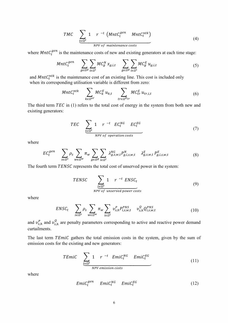
4.1. System Cost Table 3 displays the system-wide costs for the different scenarios and planning stages. In the last two planning stages, the costs associated with the “Status quo gen” and “Paralysis” cases are higher than those of the first two cohorts. This is driven primarily by emission costs.
Table 3. NPV of system-wide cost (in M€)
Scenario case Cost term Grand plan No IC Status quo gen Paralysis
2020 Investment 130 130 130 130 Emission 263 263 263 263 O&M 1355 1355 1355 1355
2025 Investment 206 206 153 152 Emission 177 177 240 240 O&M 1004 1004 1026 1026
2030 Investment 173 173 175 179 Emission 137 137 189 189 O&M 1276 1276 1294 1295
Cumulative 4721 4721 4825 4829
4.2. Optimal Installed Power Generation Mixes Figure 4 shows the optimal generation expansion outcomes in each case and time stage, which consists of only a few power production technologies: solar PV, CCGTs, onshore and offshore wind. In particular, the assumption of a 20% cost reduction in the installation cost of carbon capture and storage (CCS) technology by 2030 is not sufficient to justify investment in this technology. In 2030, the generation investment solution encompasses only offshore wind and solar PV technologies. Onshore wind investments do not take place due to the connection capacity constraint. Relaxing this and/or increasing the candidate nodes for onshore wind connections might otherwise lead to greater onshore wind expansion in 2030.
Figure 4 shows that the north-south interconnector is found out to have little effect on RES installations required to achieve the required target levels. This suggests that the interconnector has negligible impact on variable renewable curtailments. However, our analysis does not rigorously model contingencies and may therefore underestimate the potential role of the interconnector. In contrast, decommissioning the older power generation fleet leads to 1.3 GW of new CCGTs by the year 2025 in “Grand Plan” and “No IC” (but not in the other two scenarios).
In all cases, about 1.4 GW of onshore wind capacity is required by 2020 to meet the RES-E target of 40%. Solar PV investment takes place in all cases in 2030, despite the low capacity factors (approximately 10%). The total utility-scale solar PV capacity added in the last two scenarios is nearly twice that of the first two. One plausible explanation for this is the higher carbon price which is one of the factors that influence the economic viability of investing in

16
solar PV and offshore wind. Another reason could be the anticipated cost reductions with regards to the installation costs by 2030 and beyond.
Figure 4. Optimal installed capacities of new electricity generation made along the planning horizon
Figure 5. A geographical illustration of the optimal allocation of new power generation sources by 2020 (Legend: Onshore wind. The red line represents the proposed north-south
interconnector, but it is unlikely to be operational by 2020)
Figure 5 shows the optimal allocation of the new wind farms across the island for all scenarios by 2020. By 2030, however, the locations of new power generation sources varies across scenarios, especially onshore wind. This can be seen in Figure 6 and will be expanded on in further sections.
0
1000
2000
3000
Gra
nd p
lan
No
IC
Stat
us q
uo g
en
Para
lysi
s
Gra
nd p
lan
No
IC
Stat
us q
uo g
en
Para
lysi
s
Gra
nd p
lan
No
IC
Stat
us q
uo g
en
Para
lysi
s
2020 2025 2030
New
inst
alle
d ca
paci
ty (M
W)
Onshore CCGT Solar PV Offshore

17
(a) Grand plan (b) No IC
(c) Status quo gen (d) Paralysis
Figure 6. Geographical illustration of optimal allocation outcome (cumulative) of new power generation sources in each case by 2030 (Legend: Onshore wind; Offshore wind; Solar
PV; New CCGT. The red line represents the north-south interconnector)

18
Figure 7 shows the expected energy mix for the “Grand plan” case. The energy mix is largely the same for all scenarios considered in our analysis, due primarily to the fact that all cases face the same RES target. However, in the “Status que gen” and “Paralysis” cases, the 28% conventional energy comes from the existing power plants which have higher emissions than new power plants.
4.3. Implications on Emissions from Power Production Figure 8 shows the trends in average emissions across the planning stages compared with those recorded in the year 2017. Average emissions continue to fall as the time progresses in the “Grand plan” and “No IC” cases. In the remaining two cases, average emissions remain either at their corresponding 2020 level or increase slightly due to the presence of older inefficient power plants. The 2030 emission reduction target set out in Ireland’s national mitigation plan [57] is marginally met in the “Grand plan” and “No IC” cases but not the others.
Figure 8. Expected emissions from power production
0
5
10
15
20
25
2017 2020 2025 2030
Expe
cted
em
issi
ons (
MtC
O2)
Grand plan No IC Status quo gen Paralysis
Figure 7. Expected energy mix in each planning stage for the Grand plan case
0%
20%
40%
60%
80%
100%
2020 2025 2030
Expe
cted
ene
rgy
mix
Conventional Wind Hydro Biomass Solar

19
4.4. Implications on Reliability Figure 9 compares the expected energy not served (EENS) for the different scenarios. The “Grand plan” case leads to the lowest level of EENS, with the highest in the “Paralysis” case. The scenarios that include the north-south interconnector have lower EENS. Figure 10 shows the spatial distribution of EENS, most of which lies in and around Dublin, the capital city and main load centre. Demand from datacentres is also expected to be concentrated in this region. Congestion is also high in this area. It should be noted here that these results are largely dependent on the values of VOLL chosen, for both reactive and active power. The corresponding EENS costs are 593, 593, 601 and 602 M€, respecitvely.
Figure 9. A comparison of expected energy not supplied across the different cases
0
0.84
3.5
4.5
0
1
2
3
4
5
Grand plan No IC Status quo gen Paralysis
% c
hang
e in
uns
erve
d en
ergy
co
mpa
red
to "G
rand
pla
n"

20
(a) Grand plan (b) No IC
(c) Status quo gen (d) Paralysis
Figure 10. Geographical locations of expected energy not supplied (Numbers indicate the levels)

21
4.5. Implications on Network Investment Needs Congestion is one of the key indicators for network expansion requirements. We consider a transformer or a line as congested if the power flows through it exceed 90% of its nominal transfer capacity. This value can be deemed high, particularly compared to other studies, for example in [58] where any line whose flow exceeds 80% of its nominal capacity is regarded as heavily loaded or congested. However, since we allow instantaneous power transfer through a line to go up to its rated emergency capacity (which often falls between 110 and 120% of the nominal capacity), the 90% setting can be considered sufficient to capture the most congested paths in the system. Furthermore, we have assumed that flows in each transformer or line are bounded from above by the respective emergency transfer capacity. Each scenario considered here leads to different congestion outcomes. Table 4 summarises the total number of congested power system components as well as the total length of overloaded lines. The last row contains the product of the length of a line and the number of hours in a given year in which the line is congested. These three metrics indicate the level on network upgrades that may be required.
Table 4. Comparison of congestion across the cases
Cases Grand plan No IC Status quo gen Paralysis Number of components congested 142 154 151 176 Total congested length (km) 3.509 3,659 4,020 4,435 Congested length-year (km*hour/year) 9,943 10,354 13,920 15,409
Figure 11 displays the proportion of system components that are uncongested for any given number of hours under the “Grand Plan” and “Paralysis” cases. The reason behind selecting these two cases is because they lead to the lowest and highest congestion in the system, respectively. The planning stages 2025 and 2030 are chosen because the congestion in the first planning stage (2020) is not significant enough to be included in this analysis.
Figure 11. Cumulative distributions showing the extent of possible network congestion in the
Grand plan and Paralysis cases
0.760.780.8
0.820.840.860.880.9
0.920.940.960.98
1
0 1000 2000 3000 4000 5000 6000 7000 8000
cdf
Time (hours)
Grand plan 2025 Grand plan 2030 Paralysis 2030 Paralysis 2025

22
The interpretation of the results in Figure 11 is as follows. The vertical axis displays the proportion of network components that are uncongested for each number of hours in the year. Thus, 76% of the power system components will not see flows exceed 90% of their respective nominal transfer capacities at any stage under the “Paralysis” scenario, while the corresponding figure for the “Grand Plan” scenario is 82% in 2025 and 79% in 2030. This means that there are 3% (in 2025) and 6% (in 2030) more components in the “Paralysis” case that are congested at least for one hour during the respective year than in the “Grand plan” one.
A general observation is that the level of congestion in the “Paralysis” case is significantly higher than that of the “Grand plan” one. In every planning year and case, about 1% of the transformers and lines are congested for more than half of the year. Figure 12 illustrates the corridors that are heavily loaded in the year 2030 corresponding to each case. In reality, these congestion metrics are closely related with grid reinforcement requirements.

23
(a) Grand plan (b) No IC
(c) Status quo gen (d) Paralysis
Figure 12. A geographical illustration and comparison of possible network congestion in the considered cases (Note that bold lines show the corridors that are heavily congested
for more than 1000 hours per year, and overloaded transformers are not shown)

24
4.6. Implications on Renewable Power Curtailments Figure 13 compares wind power curtailment across the different cases and different stages of the planning window. The level of curtailment is relatively constant under each scenario. Furthermore, each scenario sees an increasing trend in curtailments over time from about 2% in 2020 to over 10% in 2030.
Figure 13. Expected wind power curtailment for each case and year
5. Sensitivity Analysis
5.1. Changes in SNSP Limit For security reasons, the system non-synchronous penetration (SNSP) is limited to a certain level. Currrently, the Irish power system is operated at an SNSP limit of 65%, which is expected to increase to 75% in 2020. Further increases in the SNSP limit may be possible with the advent of advanced technologies, such as energy storage systems that have the capability to provide “digital” inertia. We have therefore analysed the impact of increasing the SNSP limit from 75 to 100% under the “Grand plan” case. As noted above, this in reality need not equate to having no conventional generation units online, as up to 950 MW of conventional generation can be exported to Great Britain via the HVDC interconnectors. The results are summarised in Table 5.
Table 5. Impact of changes in the SNSP limit
Grand plan SNSP75
Grand plan SNSP85
Grand plan SNSP100
SNSP limit 75 85 100 Change in system cost (%) 0 -2 -4 Change in expected variable RES power curtailment (%) 0 -106 -596 Change in expected emissions (%) 0 +2 +4
0
5
10
15
2020 2025 2030Expe
cted
cur
tailm
ent o
f win
d po
wer
(%
)
Grand plan No IC Status quo gen Paralysis

25
The new generation capacity required by 2030 under each SNSP limit is shown in Figure 14. Total capacity investments reduce by 795 MW and 1048 MW for SNSPs of 85% and 100%, respectively. The increase in emissions observed in Table 5 is explained by the reduction in investments in new offshore wind, no investments in solar PV, and higher investments in new CCGTs..
Figure 14. Impact on installed generation capacity and technology mix in the “Grand plan” case
It should be noted here that increased deployment of energy storage and/or HVDC interconnection with other systems would likely have a similar effect to that of increased SNSP. This will be covered in future work.
5.2. Changes in Carbon Price Another model parameter that is subject to a high level of uncertainty is the price of CO2 emissions, or simply carbon price. We perform a sensitivity analysis by varying the carbon price in 2030 between 30 and 55 €/tCO2. Numerical results are presented in Figure 15 and Table 6. Figure 15 reveals no significant differences in the mix of new power generation investments in each scenario. The changes in wind power curtailments and average emissions are also not considerable in both cases. The primary impact of an increased carbon price is in system costs.
Table 6. Impact of changes in carbon price (the first column is a reference in each scenario)
Grand plan Paralysis Carbon price (€/tCO2) 20 30 45 55 20 30 45 55 Change in system cost (%) 0.0 +2.6 +6.3 +8.5 0.0 +3.5 +8.3 +11.3 Change in expected wind energy curtailment (%) 0.0 -0.6 -0.7 -1.1 0.0 -0.6 -1.4 -2.0 Changes in expected emissions (%) 0.0 -0.1 -0.1 -0.2 0.0 -0.25 -0.30 -0.32
1,267 1,373 1,405
2,440 2,440 2,440
599
1,9711,669 1,384
0
1000
2000
3000
4000
5000
6000
7000
Grand plan SNSP75 Grand plan SNSP85 Grand plan SNSP100
New
inst
alle
d ca
paci
ty (M
W)
CCGT Onshore Solar Offshore

26
Figure 15. Impact of carbon price variation on the installed generation capacity and technology mixes in the “Grand plan” and “Paralysis” cases
5.3. Changes in RES-E Integration Target Finally, we analyse the impact of different levels of RES-E integration targets. We consider various scenarios, from no RES-E target (designated as “RE eco”, which stands for RES economic) to a 60% RES-E target, (“RE60”). The actual renewable share in the “RE eco” case is about 35% for the entire island. Figure 16 shows the optimal generation mix under each target. The additional generation capacity required by 2030 increases exponentially with an increasing RES-E target. Investments in new CCGTs decrease slightly, while there are investments in large quantities of wind and solar power plants. Renewable power curtailments and system costs also increase substantially (Table 7).
Figure 16. Impact of RES-E target on the installed generation capacity and technology mix by 2030
01000200030004000500060007000
20 30 45 55 20 30 45 55
Grand plan Paralaysis
New
gen
erat
ion
capa
city
(MW
)
Carbon price and scenario
Onshore Offshore Solar CCGT
1,700 1,586 1,267 748
1,460 2,364 2,4402,440
599 1,260
1,971
5,488
0100020003000400050006000700080009000
10000
Grand plan REeco
Grand planRE40
Grand planRE50
Grand planRE60
New
inst
alle
d ca
paci
ty (M
W)
CCGT Onshore Solar Offshore

27
Table 7. Impact of changes in the RES-E target by 2030
Grand plan
RE eco Grand plan
RE40 Grand plan
RE50 Grand plan
RE60 RES-E target 35 40 50 60 Change in system cost (%) 0 +1 +11 +25 Change in expected wind energy curtailment (%) 0 -71 +55 +81 Changes in expected emissions (%) 0 -4 -16 -30
6. Conclusions and Policy Recommendations
Several of the results above have interesting implications. First and foremost, the “Grand plan” scenario leads to the lowest costs, along with the lowest emissions and highest reliability. This suggests that the decommissioning of old inefficient power generation stations is optimal from a least-cost perspective. The impact of decommissioning on carbon emissions is particularly significant, leading to a 37% reduction in 2030.
The impact of decommissioning on European emission levels, as opposed to Irish levels, is less clear. This is due to the fact that electricity generation is covered by the EU-ETS system, and there may therefore be the potential for carbon leakage. The absence of a carbon price floor across Europe increases the likelihood of carbon leakage, as the lower demand for carbon permits from generators in one jurisdiction will reduce the price of carbon permits at EU level, and therefore reduce incentives for carbon reduction elsewhere in the EU.
The north-south interconnector, in contrast, has a negligible impact on the aggregate results (whether or not decommissioning occurs). However, the locational details vary depending on whether the interconnector exists or not, particularly for expected energy not served (EENS). The interconnector’s primary function is to reduce both the number of hours and the number of locations of electricity supply interruptions. This has important implications for policy makers in determining the level of priority to award the interconnector.
The renewable generation portfolio that proves cost-optimal relies initially on onshore wind, with offshore wind and solar investments delayed until 2025 and 2030 respectively. However given the results in Figure 14, it appears that the latter investments are driven primarily by curtailment. Raising the SNSP limit or investing in storage and/or interconnection may enable very high levels of renewable generation to be reached with lower levels of these more expensive renewable technologies.
At the high levels of RES that Ireland has targeted, increased carbon prices have little effect other than to increase total costs. This suggests that the RES targets that have been set for the Irish system are at least equal to those that would prove optimal under the carbon prices assumed in this work, and may be higher. Policy makers should be aware of the potential for one policy measure (e.g. a renewable target) to render another measure (e.g. a carbon price signal) irrelevant. Therefore, they should exercise caution in investing or political capital or other resources in mutually inclusive policies simultaneously.

28
Nomenclature
Indices and Sets 𝑔𝑔/Ω𝑔𝑔 Index/set of all generators (existing and new) 𝑀𝑀, 𝑗𝑗/Ω𝑖𝑖 Index/set of all nodes 𝑀𝑀′ Index for fictitious transformer node 𝑘𝑘/Ω𝑛𝑛 Index/set of all lines 𝑀𝑀/Ω𝑡𝑡 Index/set of time stages 𝑀𝑀𝑟𝑟/Ω𝐸𝐸𝑡𝑡𝑡𝑡 Index/set of existing transformers 𝑐𝑐/Ω𝑖𝑖 Index/set of storylines (scenarios) 𝑤𝑤,𝑤𝑤′/Ω𝑤𝑤 Index/set of operational states Ω𝑅𝑅𝐸𝐸𝑃𝑃 Set of all RES type power generators Ω𝑔𝑔ℓ Set of existing lines
Functions 𝑇𝑇𝑇𝑇𝑡𝑡
𝑔𝑔𝑔𝑔𝑔𝑔 Cost of energy generated by all generators (€) 𝑇𝑇𝑇𝑇𝑡𝑡𝑁𝑁𝑁𝑁 Cost of energy generated by new generators (€) 𝑇𝑇𝑇𝑇𝑡𝑡𝐸𝐸𝑁𝑁 Cost of energy generated by existing generators (€) 𝑇𝑇𝑇𝑇𝑇𝑇𝑇𝑇𝑡𝑡 Cost of unserved energy (€) 𝑇𝑇𝑀𝑀𝑀𝑀𝑇𝑇𝑡𝑡
𝑔𝑔𝑔𝑔𝑔𝑔 Emission cost associated to all generators (€) 𝑇𝑇𝑀𝑀𝑀𝑀𝑇𝑇𝑡𝑡𝑁𝑁𝑁𝑁 Emission cost associated to new generators (€) 𝑇𝑇𝑀𝑀𝑀𝑀𝑇𝑇𝑡𝑡𝐸𝐸𝑁𝑁 Emission cost associated to existing generators (€) 𝑇𝑇𝑀𝑀𝑇𝑇𝑇𝑇𝑡𝑡
𝑔𝑔𝑔𝑔𝑔𝑔 Investment cost in generators (€) 𝑀𝑀𝑀𝑀𝑀𝑀𝑇𝑇𝑡𝑡
𝑔𝑔𝑔𝑔𝑔𝑔 Maintenance cost associated with all generators (€) 𝑀𝑀𝑀𝑀𝑀𝑀𝑇𝑇𝑡𝑡𝑔𝑔𝑡𝑡𝑛𝑛 Maintenance cost associated with network components(€)
Parameters 𝑏𝑏𝑛𝑛0 Shunt susceptance of a line (pu) 𝑏𝑏𝑛𝑛 Susceptance of a line (pu) 𝑇𝑇𝐸𝐸𝑔𝑔𝑁𝑁 Emission rate of a new generator (tons of CO2e/MWh) 𝑇𝑇𝐸𝐸𝑔𝑔𝐸𝐸 Emission rate of an existing generator (tons of CO2e/MWh) 𝑔𝑔𝑛𝑛 Conductance of a line (pu) 𝐿𝐿𝑇𝑇𝑔𝑔 Lifetime of a generator (years) 𝐿𝐿𝑇𝑇𝑡𝑡𝑟𝑟 Lifetime of a transformer (years) 𝑇𝑇𝑇𝑇𝑔𝑔,𝑖𝑖 Capital cost of a generator (€) 𝑀𝑀𝑇𝑇𝑔𝑔𝑁𝑁 Maintenance cost of a new generator (€/year) 𝑀𝑀𝑇𝑇𝑔𝑔𝐸𝐸 Maintenance cost of an existing generator (€/year) 𝑀𝑀𝑇𝑇𝑛𝑛𝑁𝑁 Maintenance cost of a new line (€/year) 𝑀𝑀𝑇𝑇𝑛𝑛𝐸𝐸 Maintenance cost of an existing line (€/year) 𝑀𝑀𝑇𝑇𝑡𝑡𝑟𝑟𝑁𝑁 Maintenance cost of a new transformer (€/year) 𝑀𝑀𝑇𝑇𝑡𝑡𝑟𝑟𝐸𝐸 Maintenance cost of an existing transformer (€/year) 𝑀𝑀𝑄𝑄𝑛𝑛 Big-M (disjunctive) parameter

29
𝑀𝑀𝑃𝑃𝑛𝑛 Big-M (disjunctive) parameter 𝑇𝑇𝑤𝑤 Number of operational states 𝑃𝑃𝑃𝑃𝑖𝑖,𝑤𝑤,𝑡𝑡
𝑖𝑖,0 Active power demand without DR program (MW) 𝑟𝑟 Interest rate (%) 𝑄𝑄𝑃𝑃𝑖𝑖,𝑤𝑤
𝑖𝑖,0 Reactive power demand without DR program (MVAr) 𝐸𝐸𝑡𝑡𝑟𝑟, 𝑋𝑋𝑡𝑡𝑟𝑟 Resistance, reactance of transformer (pu) 𝐸𝐸𝑛𝑛 Resistance of a line (pu) 𝑇𝑇𝐵𝐵 Base power (MVA) 𝑇𝑇𝑡𝑡𝑟𝑟𝑖𝑖𝑚𝑚𝑚𝑚 Maximum apparent power flow through transformer (MVA) 𝑇𝑇𝑛𝑛𝑖𝑖𝑚𝑚𝑚𝑚 Maximum apparent power flow through line (MVA) 𝑇𝑇 Duration of the planning horizon (years) 𝑋𝑋𝑛𝑛 Reactance of a line (pu) ∆𝑉𝑉𝑖𝑖𝑚𝑚𝑚𝑚, ∆𝑉𝑉𝑖𝑖𝑖𝑖𝑔𝑔 Upper and lower limits of voltage deviations (pu) 𝜆𝜆𝑔𝑔,𝑖𝑖,𝑤𝑤,𝑡𝑡𝑁𝑁𝑁𝑁 Marginal operation cost of a new generator (€/MWh) 𝜆𝜆𝑔𝑔,𝑖𝑖,𝑤𝑤,𝑡𝑡𝐸𝐸𝑁𝑁 Marginal operation cost of an existing generator(€/MWh) 𝜆𝜆𝑖𝑖,𝑤𝑤,𝑡𝑡𝐶𝐶𝐶𝐶2𝑔𝑔 Unit cost of emissions (€/tons of CO2e) 𝜐𝜐𝑖𝑖,ℎ𝑁𝑁 Penalty for load shedding (€/MW) 𝜐𝜐𝑖𝑖,ℎ𝑄𝑄 Penalty for load shedding (€/MVAr) 𝜉𝜉𝑤𝑤,𝑤𝑤′ Price elasticity of demand 𝜋𝜋𝑤𝑤 Weight associated to representative operational state 𝜌𝜌𝑖𝑖 Probability of realization of a storyline (scenario) 𝜓𝜓 DR penetration level
Variables 𝑃𝑃𝑛𝑛,𝑖𝑖,𝑤𝑤,𝑡𝑡 Active power flows in a branch (MW) 𝑃𝑃𝑔𝑔,𝑖𝑖,𝑖𝑖,𝑤𝑤,𝑡𝑡𝑔𝑔𝑔𝑔𝑔𝑔 Active power production (MW)
𝑃𝑃𝑔𝑔,𝑖𝑖,𝑖𝑖,𝑤𝑤,𝑡𝑡𝑁𝑁 Active power production by new generator (MW)
𝑃𝑃𝑔𝑔,𝑖𝑖,𝑖𝑖,𝑤𝑤,𝑡𝑡𝐸𝐸 Active power production by existing generator (MW)
𝑃𝑃𝑖𝑖,𝑖𝑖,𝑤𝑤,𝑡𝑡𝑁𝑁𝑁𝑁𝑃𝑃 Unserved active power (MW)
𝑃𝑃𝑃𝑃𝑖𝑖,𝑤𝑤,𝑡𝑡𝑖𝑖 Active power demand with DR program (MW)
𝑃𝑃𝐿𝐿𝑛𝑛,𝑖𝑖,𝑤𝑤,𝑡𝑡, 𝑄𝑄𝐿𝐿𝑛𝑛,𝑖𝑖,𝑤𝑤,𝑡𝑡 Active, reactive power losses (MW, MVAr) 𝑃𝑃𝑡𝑡𝑟𝑟,𝑖𝑖,𝑤𝑤,𝑡𝑡 Active power flow through a transformer (MW) 𝑃𝑃𝑡𝑡𝑟𝑟,𝑖𝑖,𝑤𝑤,𝑡𝑡 Reactive power flow through a transformer (MVAr) 𝑃𝑃𝑛𝑛,𝑖𝑖,𝑤𝑤,𝑡𝑡+ ,𝑃𝑃𝑛𝑛,𝑖𝑖,𝑤𝑤,𝑡𝑡
− Auxiliary active power flow variables (MW) 𝑄𝑄𝑔𝑔,𝑖𝑖,𝑖𝑖,𝑤𝑤,𝑡𝑡𝑔𝑔𝑔𝑔𝑔𝑔 Reactive power production (MVAr)
𝑄𝑄𝑛𝑛,𝑖𝑖,𝑤𝑤,𝑡𝑡 Reactive power flows in a branch (MVAr) 𝑄𝑄𝑖𝑖,𝑖𝑖,𝑤𝑤,𝑡𝑡𝑁𝑁𝑁𝑁𝑃𝑃 Unserved reactive power (MVAr)
𝑄𝑄𝑃𝑃𝑖𝑖,𝑤𝑤,𝑡𝑡𝑖𝑖 Active power demand with DR program (MVAr)

30
𝑄𝑄𝑛𝑛,𝑖𝑖,𝑤𝑤,𝑡𝑡+ ,𝑄𝑄𝑛𝑛,𝑖𝑖,𝑤𝑤,𝑡𝑡
− Auxiliary reactive power flow variables (MVAr)
𝑄𝑄𝑖𝑖,𝑖𝑖,𝑤𝑤,𝑡𝑡𝑟𝑟𝑖𝑖 Reactive power injected/absorbed at node i by a capacitor/reactor
(MVAr) 𝑥𝑥𝑔𝑔,𝑖𝑖,𝑡𝑡 Generator investment variable ∆𝑉𝑉𝑖𝑖,𝑖𝑖,𝑤𝑤,𝑡𝑡 Voltage deviation at a node (pu) ∆𝑀𝑀𝑡𝑡𝑟𝑟 Change in turns ratio per tap ∆𝑄𝑄𝑛𝑛,𝑖𝑖,𝑤𝑤,𝑡𝑡,𝑙𝑙 Step-size flow variable (MVAr) ∆𝑃𝑃𝑛𝑛,𝑖𝑖,𝑤𝑤,𝑡𝑡,𝑙𝑙 Step-size flow variable (MW) 𝜃𝜃𝑛𝑛,𝑖𝑖,𝑤𝑤,𝑡𝑡 Angle difference along transmission end points (radians) 𝜃𝜃𝑖𝑖,𝑖𝑖,𝑤𝑤,𝑡𝑡 Voltage angle at node i (radians)
Appendices
Appendix A. Parameters
Table A.1. Parameter assumptions of generators (existing and candidate alike) [59]–[61]
Generation technology
Operation cost
(€/MWh)
Emission rate (tCO2/MWh)
Investment cost
(M€/MW)
Cost reductions (cumulative)
2020 2025 2030 Offshore wind 22.8 0.015 3.65 0.05 0.10 0.20 Onshore wind 13.0 0.015 1.40 0.05 0.10 0.20 Solar PV 11.4 0.046 1.50 0.05 0.10 0.20 Biomass 54.0 0.230 2.25 0.02 0.05 0.10 Coal 34.0 0.925 0.90 0.05 0.08 0.10 Coal with CCS 38.0 0.185 4.40 0.05 0.08 0.10 CCGT 40.0 0.367 0.90 0.05 0.08 0.10 CCGT with CCS
55.0
0.037 2.40 0.05 0.08 0.10
Hydro 10.5 0.010 - - - - Gas oil fired 80.0 1.041 - - - - Heavy fuel oil fired
100.0
0.769 - - - -

31
References
[1] C. L. Quéré et al., “Global Carbon Budget 2018,” Earth Syst. Sci. Data, vol. 10, no. 4, pp. 2141–2194, Dec. 2018.
[2] Intergovernmental Panel on Climate Change, Global warming of 1.5°C. 2018. [3] L. Gacitua et al., “A comprehensive review on expansion planning: Models and tools for energy
policy analysis,” Renew. Sustain. Energy Rev., vol. 98, pp. 346–360, Dec. 2018. [4] S. Chen, Z. Guo, P. Liu, and Z. Li, “Advances in clean and low-carbon power generation
planning,” Comput. Chem. Eng., vol. 116, pp. 296–305, Aug. 2018. [5] N. E. Koltsaklis and A. S. Dagoumas, “State-of-the-art generation expansion planning: A
review,” Appl. Energy, vol. 230, pp. 563–589, Nov. 2018. [6] V. Oree, S. Z. Sayed Hassen, and P. J. Fleming, “Generation expansion planning optimisation
with renewable energy integration: A review,” Renew. Sustain. Energy Rev., vol. 69, pp. 790–803, Mar. 2017.
[7] B. Palmintier and M. Webster, “Impact of operational flexibility on electricity generation planning with renewable and carbon targets,” in 2016 IEEE Power and Energy Society General Meeting (PESGM), 2016, pp. 1–1.
[8] S. A. Rashidaee, T. Amraee, and M. Fotuhi-Firuzabad, “A Linear Model for Dynamic Generation Expansion Planning Considering Loss of Load Probability,” IEEE Trans. Power Syst., vol. 33, no. 6, pp. 6924–6934, Nov. 2018.
[9] J. Aghaei, N. Amjady, A. Baharvandi, and M.-A. Akbari, “Generation and Transmission Expansion Planning: MILP - Based Probabilistic Model,” IEEE Trans. Power Syst., vol. 29, no. 4, pp. 1592–1601, Jul. 2014.
[10] D. Pozo, E. E. Sauma, and J. Contreras, “A Three-Level Static MILP Model for Generation and Transmission Expansion Planning,” IEEE Trans. Power Syst., vol. 28, no. 1, pp. 202–210, Feb. 2013.
[11] J. H. Roh, M. Shahidehpour, and Y. Fu, “Market-Based Coordination of Transmission and Generation Capacity Planning,” IEEE Trans. Power Syst., vol. 22, no. 4, pp. 1406–1419, Nov. 2007.
[12] R. Hemmati, R.-A. Hooshmand, and A. Khodabakhshian, “Coordinated generation and transmission expansion planning in deregulated electricity market considering wind farms,” Renew. Energy, vol. 85, pp. 620–630, Jan. 2016.
[13] A. H. Seddighi and A. Ahmadi-Javid, “Integrated multiperiod power generation and transmission expansion planning with sustainability aspects in a stochastic environment,” Energy, vol. 86, pp. 9–18, Jun. 2015.
[14] N. Zhang, Z. Hu, C. Springer, Y. Li, and B. Shen, “A bi-level integrated generation-transmission planning model incorporating the impacts of demand response by operation simulation,” Energy Convers. Manag., vol. Complete, no. 123, pp. 84–94, 2016.
[15] O. J. Guerra, D. A. Tejada, and G. V. Reklaitis, “An optimization framework for the integrated planning of generation and transmission expansion in interconnected power systems,” Appl. Energy, vol. 170, pp. 1–21, May 2016.
[16] H. Saboori and R. Hemmati, “Considering Carbon Capture and Storage in Electricity Generation Expansion Planning,” IEEE Trans. Sustain. Energy, vol. 7, no. 4, pp. 1371–1378, Oct. 2016.
[17] S. Pineda and J. M. Morales, “Chronological Time-Period Clustering for Optimal Capacity Expansion Planning With Storage,” IEEE Trans. Power Syst., vol. 33, no. 6, pp. 7162–7170, Nov. 2018.
[18] A. Bhuvanesh, S. T. Jaya Christa, S. Kannan, and M. Karuppasamy Pandiyan, “Aiming towards pollution free future by high penetration of renewable energy sources in electricity generation expansion planning,” Futures, vol. 104, pp. 25–36, Dec. 2018.
[19] T. Luz, P. Moura, and A. de Almeida, “Multi-objective power generation expansion planning with high penetration of renewables,” Renew. Sustain. Energy Rev., vol. 81, pp. 2637–2643, Jan. 2018.

32
[20] N. van Bracht and A. Moser, “Generation expansion planning under uncertainty considering power-to-gas technology,” in 2017 14th International Conference on the European Energy Market (EEM), 2017, pp. 1–6.
[21] A. Sarid and M. Tzur, “The multi-scale generation and transmission expansion model,” Energy, vol. 148, pp. 977–991, Apr. 2018.
[22] P. J. Ramírez, D. Papadaskalopoulos, and G. Strbac, “Co-Optimization of Generation Expansion Planning and Electric Vehicles Flexibility,” IEEE Trans. Smart Grid, vol. 7, no. 3, pp. 1609–1619, May 2016.
[23] M. Peker, A. S. Kocaman, and B. Y. Kara, “A two-stage stochastic programming approach for reliability constrained power system expansion planning,” Int. J. Electr. Power Energy Syst., vol. 103, pp. 458–469, Dec. 2018.
[24] S. Pereira, P. Ferreira, and A. I. F. Vaz, “Generation expansion planning with high share of renewables of variable output,” Appl. Energy, vol. 190, pp. 1275–1288, Mar. 2017.
[25] H. Park and R. Baldick, “Multi-year stochastic generation capacity expansion planning under environmental energy policy,” Appl. Energy, vol. 183, pp. 737–745, Dec. 2016.
[26] V. Slednev, V. Bertsch, M. Ruppert, and W. Fichtner, “Highly resolved optimal renewable allocation planning in power systems under consideration of dynamic grid topology,” Comput. Oper. Res., vol. 96, pp. 281–293, Aug. 2018.
[27] H. Fathtabar, T. Barforoushi, and M. Shahabi, “Dynamic long-term expansion planning of generation resources and electric transmission network in multi-carrier energy systems,” Int. J. Electr. Power Energy Syst., vol. 102, pp. 97–109, Nov. 2018.
[28] A. J. C. Pereira and J. T. Saraiva, “Generation expansion planning (GEP) – A long-term approach using system dynamics and genetic algorithms (GAs),” Energy, vol. 36, no. 8, pp. 5180–5199, Aug. 2011.
[29] Y. Zhan, Q. P. Zheng, J. Wang, and P. Pinson, “Generation Expansion Planning With Large Amounts of Wind Power via Decision-Dependent Stochastic Programming,” IEEE Trans. Power Syst., vol. 32, no. 4, pp. 3015–3026, Jul. 2017.
[30] K. Poncelet, H. Höschle, E. Delarue, A. Virag, and W. D’haeseleer, “Selecting Representative Days for Capturing the Implications of Integrating Intermittent Renewables in Generation Expansion Planning Problems,” IEEE Trans. Power Syst., vol. 32, no. 3, pp. 1936–1948, May 2017.
[31] M. D. Rodgers, D. W. Coit, F. A. Felder, and A. Carlton, “Generation expansion planning considering health and societal damages – A simulation-based optimization approach,” Energy, vol. 164, pp. 951–963, Dec. 2018.
[32] C. F. Heuberger, E. S. Rubin, I. Staffell, N. Shah, and N. Mac Dowell, “Power capacity expansion planning considering endogenous technology cost learning,” Appl. Energy, vol. 204, pp. 831–845, Oct. 2017.
[33] D. Jornada and V. J. Leon, “Robustness methodology to aid multiobjective decision making in the electricity generation capacity expansion problem to minimize cost and water withdrawal,” Appl. Energy, vol. 162, pp. 1089–1108, Jan. 2016.
[34] H. Chen, B.-J. Tang, H. Liao, and Y.-M. Wei, “A multi-period power generation planning model incorporating the non-carbon external costs: A case study of China,” Appl. Energy, vol. 183, pp. 1333–1345, Dec. 2016.
[35] M. Gitizadeh, M. Kaji, and J. Aghaei, “Risk based multiobjective generation expansion planning considering renewable energy sources,” Energy, vol. 50, pp. 74–82, Feb. 2013.
[36] F. Chen, G. Huang, and Y. Fan, “A linearization and parameterization approach to tri-objective linear programming problems for power generation expansion planning,” Energy, vol. 87, pp. 240–250, Jul. 2015.
[37] N. E. Koltsaklis and M. C. Georgiadis, “A multi-period, multi-regional generation expansion planning model incorporating unit commitment constraints,” Appl. Energy, vol. 158, pp. 310–331, Nov. 2015.
[38] M. A. Abido, “Environmental/economic power dispatch using multiobjective evolutionary algorithms,” IEEE Trans. Power Syst., vol. 18, no. 4, pp. 1529–1537, Nov. 2003.
[39] D. Z. Fitiwi, “Strategies, methods and tools for solving long-term transmission expansion planning in large-scale power systems,” 2016.

33
[40] D. Z. Fitiwi, S. F. Santos, C. M. P. Cabrita, and J. P. S. Catalão, “Stochastic mathematical model for high penetration of renewable energy sources in distribution systems,” in 2017 IEEE Manchester PowerTech, 2017, pp. 1–6.
[41] D. Z. Fitiwi, L. Olmos, M. Rivier, F. de Cuadra, and I. J. Pérez-Arriaga, “Finding a representative network losses model for large-scale transmission expansion planning with renewable energy sources,” Energy, vol. 101, pp. 343–358, abril 2016.
[42] V. Bertsch, M. Devine, C. Sweeney, and A. C. Parnell, “Analysing long-term interactions between demand response and different electricity markets using a stochastic market equilibrium model,” Economic and Social Research Institute (ESRI), WP585, 2018.
[43] M. G. Bosilovich, R. Lucchesi, and M. Suarez, “MERRA-2: File Specification. GMAO Office Note,” 2016. [Online]. Available: https://gmao.gsfc.nasa.gov/reanalysis/MERRA-2/. [Accessed: 11-Dec-2018].
[44] S. F. Santos, D. Z. Fitiwi, M. Shafie-khah, A. W. Bizuayehu, C. M. P. Cabrita, and J. P. S. Catalão, “New Multi-Stage and Stochastic Mathematical Model for Maximizing RES Hosting Capacity - Part II: Numerical Results,” IEEE Trans. Sustain. Energy, vol. 8, no. 1, pp. 320–330, Jan. 2017.
[45] H. W. Qazi and D. Flynn, “Analysing the impact of large-scale decentralised demand side response on frequency stability,” Int. J. Electr. Power Energy Syst., vol. 80, pp. 1–9, setembro 2016.
[46] EirGrid, “Smart Grid Dashboard,” EirGrid Smart Grid Dashboard. [Online]. Available: http://smartgriddashboard.eirgrid.com/. [Accessed: 11-Dec-2018].
[47] J. Hartigan and M. Wong, “Algorithm AS 136: A k-means clustering algorithm,” Appl. Stat., vol. 28, no. 1, pp. 100–108, 1979.
[48] EirGrid, “Tomorrow’s Energy Scenarios 2017: Planning our Energy Future,” 2017. [49] F. Desta Zahlay, “Strategy, Methods and Tools for Solving Long-term Transmission Expansion
Planning in Large-scale Power Systems,” Comillas Pontifical University, 2016. [50] GAMS, “General Algebraic Modeling System Software,” 2018. [Online]. Available:
https://www.gams.com/. [Accessed: 11-Dec-2018]. [51] CPLEX 12, “CPLEX User’s Manual,” p. 564, 2015. [52] EirGrid, “All-Island TenYear Transmission Forecast Statement 2016,” 2016. [53] E. Leahy and R. S. J. Tol, “An estimate of the value of lost load for Ireland,” Energy Policy,
vol. 39, no. 3, pp. 1514–1520, Mar. 2011. [54] Carbon Tracker, “EU carbon prices could double by 2021 and quadruple by 2030,” Carbon
Tracker Initiative, 26-Apr-2018. [Online]. Available: https://www.carbontracker.org/eu-carbon-prices-could-double-by-2021-and-quadruple-by-2030/. [Accessed: 11-Dec-2018].
[55] EirGrid and SONI, “System Non-Synchronous Penetration, Definition and Formulation: Operational Policy.” Aug-2018.
[56] EirGrid and SONI, “All-Island TSO Facilitation of Renewables Studies,” Jun. 2010. [57] DCCAE, “National Mitigation Plan,” Jul. 2017. [58] Desta Z. Fitiwi, F. de Cuadra, L. Olmos, and M. Rivier, “A new approach of clustering
operational states for power network expansion planning problems dealing with RES (renewable energy source) generation operational variability and uncertainty,” Energy, vol. 90, no. 2, pp. 1360–1376, Oct. 2015.
[59] SEAI, “Energy-Related Emissions in Ireland: CO2 Emissions from Fuel Combustion.” 2016. [60] IRENA, “Renewable power generation costs in 2017,” 2017. [61] IEA, “Projected Costs of Generating Electricity 2015 Edition,” p. 215, 2015.

Year Number Title/Author(s) 2019 615 The effects of spatial position of calorie information on
choice, consumption and attention Deirdre A. Robertson, Pete Lunn
614 The determinants of SME capital structure across the lifecycle Maria Martinez-Cillero, Martina Lawless, Conor O’Toole
612 Can official advice improve mortgage-holders’ perceptions of switching? An experimental investigation Shane Timmons, Martina Barjaková, Terence J. McElvaney, Pete Lunn
611 Underestimation of money growth and pensions: Experimental investigations Féidhlim P. McGowan, Pete Lunn, Deirdre A. Robertson
610 Housing Assistance Payment: Potential impacts on financial incentives to work Barra Roantree, Mark Regan, Tim Callan, Michael Savage, John R. Walsh
609 Predicting farms’ noncompliance with regulations on nitrate pollution Pete Lunn, Seán Lyons and Martin Murphy
2018 608 How openness to trade rescued the Irish economy
Kieran McQuinn, Petros Varthalitis 607 Senior cycle review: Analysis of discussion in schools on
the purpose of senior cycle education in Ireland Joanne Banks, Selina McCoy, Emer Smyth
606 LNG and gas storage optimisation and valuation: Lessons from the integrated Irish and UK markets Mel T. Devine, Marianna Russo
605 The profitability of energy storage in European electricity markets Petr Spodniak, Valentin Bertsch, Mel Devine
604 The framing of options for retirement: Experimental tests for policy Féidhlim McGowan, Pete Lunn, Deirdre Robertson
603 The impacts of demand response participation in capacity markets Muireann Á. Lynch, Sheila Nolan, Mel T. Devine, Mark O'Malley
602 Review of the Irish and international literature on health and social care unit cost methodology Richard Whyte, Conor Keegan, Aoife Brick, Maev-Ann Wren
For earlier Working Papers see http://ww.esri.ie


![[XLS] · Web view74839 6 61 616 6160 74840 6 61 616 6160 74850 6 61 616 6160 74860 6 61 616 6160 74877 6 61 616 6160 74890 6 61 616 6160 74911 6 61 616 6160 74912 6 61 616 6160 74913](https://static.fdocuments.net/doc/165x107/5ae388b97f8b9a7b218d329b/xls-view74839-6-61-616-6160-74840-6-61-616-6160-74850-6-61-616-6160-74860-6-61.jpg)