Working Paper No. 143

Investment Climate and Economic Performance: Some Firm Level Evidence

from India∗∗∗ ∗

by

David Dollar Giuseppe Iarossi Taye Mengistae

May 2002

∗ The findings and interpretations expressed in this paper are those of the authors and do not necessarilyreflect official views of the World Bank, the members of its Board of Executive Directors, or the countriesthey represent.

Stanford University John A. and Cynthia Fry Gunn Building

366 Galvez Street | Stanford, CA | 94305-6015

1

1. Introduction

Arguably the most important development in the world economy in the past two

decades is that major developing countries, including the two largest (China and India),

have altered their strategies and begun to integrate more actively with the global

economy. Developing countries that are actively integrating are getting good results, on

average. In the 1990s the top one-third of developing countries, in terms of increased

trade integration, grew at about 5% per capita, while the rich countries grew at about 2%,

and the rest of the developing world had negative growth (Dollar and Kraay, 2001). This

group of countries that is participating more in trade includes India, China, Thailand,

Brazil, Mexico, the Philippines, and Argentina. It is also well known that capital flows to

the developing world are heavily concentrated in twelve countries, and it is very much

the same list of countries.

That the developing countries that are integrating with the global economy are

doing well on average disguises the fact that there is considerable variation in

performance among this group. China has done spectacularly well. Thailand was

growing very rapidly until its financial crisis, and now seems to be rebounding quickly

from that. Mexico is doing well with its growing integration with the U.S. economy.

Brazil, on the other hand, has only been growing at about 2%, and the Philippines, at 3%,

in the second half of the 1990s. India, with per capita growth of 4.4% in the late 1990s,

is about in the middle of the pack, for the large, globalizing economies. Furthermore,

there is large variation in performance across locations within these countries. Chinese

2

coastal areas are booming, while much of the interior is not. In both Mexico and India,

there are rapidly growing states and stagnating ones.

The basic question that we address in this paper is to what extent differences in

performance across locations depends on differences in the investment climate – by

which we mean the regulatory environment for firms and the quality of infrastructure,

which itself traces back to a large extent to public regulation? Also, if the investment

climate is important, what are the specific aspects of the investment climate that are the

main bottlenecks? We are going to address these questions using a new, firm-level data-

base from India. The survey covers 1,032 firms from the manufacturing sector, as well as

the software industry. The survey was carried out by the Confederation of Indian

Industries and the World Bank and covers ten Indian states: Maharashtra, Gujarat,

Andhra Pradesh, Karnataka, Tamil Nadu, Punjab, Delhi, Kerala, West Bengal, and Uttar

Pradesh.1

It is useful to begin by discussing in more detail what we mean by the

“investment climate.” The quantity and quality of investment in India or any other

developing country depends on the returns that investors expect and the uncertainties

around those returns. It is useful to think of three broad and interrelated components that

shape these expectations.

1 The selection of states was based on three principles. The first was that the sample should be spread asmuch as possible between high-income states, middle-income states and poorer states. Secondly, thesample should represent what, at the time of the survey, were seen to be reforming states as well as stateswhose policy environment was not thought to be so friendly to business. The third principle was that a stateshould have a sizable number of establishments in at least three of the industries the survey was intended tocover. Based on the World Bank’s classification (World Bank, 1999), the states of Delhi, Maharasthtra,Gujarat, Punjab and West Bengal represent the high-income group of states. Uttar Pradesh is a low-incomestate while Andra Pradesh, Karnataka, Kerala and Tamil Nadu represent middle income states. Per capitaincome averaged Rs 4377 in high-income states in 1996-97 at 1980 prices against Rs 2676 in middle-income states and Rs 1840 in low-income states.

3

First, there are macro or country-level issues concerning economic and political

stability and nationwide policy toward foreign trade and investment. Here, India has

clearly improved its policies over the past decade; macro-level economic reforms

contributed to the high growth of the 1990s. Relative macroeconomic and political

stability, trade liberalization plus further commitments within the WTO — these

comprise one crucial set of ingredients to spur investment and productivity growth.

These are national level and hence held constant across Indian states.

But creating a good climate for investment involves two other factors as well: (1)

the policy and regulatory framework for investment and production and (2) basic

infrastructure (power, transport, telecommunications). It is common for developing

countries to start with the macro reforms, which often produce good results compared to

past performance. However, if one does not move ahead on the institutional and

infrastructure agenda, the growth generated by macro reform is likely to peter out. It is

now broadly recognized within India that the country has reached a crucial point where

the challenge is to move forward on the institutional and infrastructure agenda

(Ahluwalia, 2001).

The policies and regulations for firms in competitive industries cover the issues of

entry (starting a business), labor relations (hiring and firing), efficiency of taxation, and

efficiency of regulations concerning the environment, safety, health, and other legitimate

public interests. These issues are regulated in all market economies, so the issue is not

whether to regulate or not. Rather, the issue is whether regulations serve the public

4

interest and are implemented efficiently without harassment and corruption.2 While these

things are hard to measure, there is evidence that we will present suggesting that the

efficiency with which production is regulated varies widely across Indian states. Our

hypothesis is that in locations with good investment climates you get more investment,

more efficient investment, and ultimately more job creation and poverty reduction.

The third key aspect of the investment climate is infrastructure, broadly defined.3

When one surveys entrepreneurs about their problems and bottlenecks, they will often

cite infrastructure issues such as power reliability, transport time and cost, and access and

efficiency of finance. It is useful to recognize that the underlying issue here is once again

policies and regulations and how they are implemented. The distinctive feature of the

infrastructure industries and the financial sector is that there are important externalities in

production so that regulation of these industries is more complicated than, say, regulation

of the garment industry. The garment industry is inherently competitive, especially in an

economy open to the world market. For power distribution, surface telephone service,

seaports, and airports, there is, on the other hand, a tendency toward local monopoly. In

the financial sector there is also a trend toward large firms that can diversify risk. There

2 In India, as in many other developing countries, business people complain that enforcement is toodiscretionary, which is a source of corruption and harassment (Ahluwalia, 1999). The cost that businessesincur in consequence seems also seems to vary considerably between Indian states.3 There is a well known and sizeable body of literature on the role of public provision of infrastructure inaggregate growth and productivity. Quite a few papers report that publicly provided infrastructure has beena major source of growth in developed and developing economies alike (e.g., Aschaure, 1989; Brendt andHansson, 1992; Munnel , 1990; Nadirir and Mamuneas, 1994; and Morrison and Shwartz, 1996) whileothers contest this view arguing that the effect of infrastructural investment on aggregagte output is at bestnegligble (e.g., Hulten and Schwab, 1991; Easterly and Rebelo, 1993; Holtz-Eakin, 1994; and Barro andSala-I-Martin, 1995). One of the causes for this ambiguity of findings seems to be dependence of thestudies on the estimationg of aggregate production functions in the context of which the problem of reversecausality on income levels and infrastructure inevitabily arises and is difficult to resolve. One of theadvantages of the use of firm level data is that the provision of infrastuructural services can reasonablyassumed to be exogenous from the perspective of any particular producer. See Reinika and Svenensson(1999) for an earlier study of the impact of public provision of infrastructure on private investment basedon establishment level data.

5

are further problems of moral hazard and adverse selection, so that financial markets left

unregulated tend toward boom and bust cycles that are extremely disruptive.

Because of the obvious importance of infrastructure and the financial sector,

many developing countries have tried to keep these services in the public sector. Results,

however, have typically not been good. Public ownership has often led to pricing below

cost so that the provision of these services put huge burdens on the public coffers.4 In

addition, political considerations have come into the allocation of finance and other

subsidized services, and these political allocations are usually not the most efficient ones

in terms of promoting growth and poverty reduction. Experience shows that, with the

right regulatory framework, one can get private investors to efficiently provide power,

telecommunication, and much of transport infrastructure (seaport and airport operations,

for example). Organizing these markets is not easy, however (witness the problems of

highly developed California, which made something of a mess of power deregulation and

in 2001 faced the same kind of power rationing that one often finds in less developed

locations). So, we observe large differences across locations in the quality of

infrastructure services.

Our investigation of the importance of the investment climate for outcomes in

India will proceed as follows: In the next section we look at entrepreneurs’ subjective

4 For example, in India, power generation and distribution was a monopoly of government ownedenterprises under State Electricity Boards (SEBs) up until the early 1990’s. For a long time now, SEBshave followed a deliberate policy of under pricing the supply of electricity to households and farms, onlypart of which they have managed to pass to industry through tariffs well above cost and international ratesThis and the boards’ growing failure to protect transmission and collect bills, has led to serious underinvestment in maintenance and capacity. Recent effort at attracting private investment as a solution includethe opening up of generation and distribution to private capital and the unbundling of SEB’s intoindependent commercial agencies specializing in generation, transmission or distribution only. In moststates these efforts have yet to bear fruit partly because of the absence of a regulatory framework in whichpotential investors have confidence. Meanwhile growing pressure on the existing productive capacity of the

6

assessment of the investment climate in different states and their estimate of the costs of

these impediments. We recognize that this information is subjective, but it provides a

benchmark ranking of states in terms of investment climate. In Section 3 we provide our

analytical framework for estimating differences in productivity across firms and for

linking productivity differences to objective measures of bottlenecks. Section 4 describes

our data. In Section 5 we show that the states identified as having better investment

climates in the subjective assessments, in fact have higher labor and total factor

productivity at the firm level. The TFP differences are very close to the estimated cost

differentials that we obtained from the entrepreneurs. Finally, in Section 6 we show that

the productivity differentials can be linked to specific objective bottlenecks such as

reliability of the power supply, the frequency of visits from government officials, time to

clear goods from customs, and other measures. Section 7 concludes.

2. Entrepreneurs’ Perception of Investment Climate

Our data come from the Firm Analysis and Competitiveness Survey (FACS) of

India, which was carried out in March-November 2000, and covered eight of India’s

main export industries, namely, textiles, garments, pharmaceuticals, electronics, electrical

white goods, auto-components, machine tools and software production. The survey

instrument was a written questionnaire addressed to business managers and accountants.

It was designed with the aim of capturing the interaction between investment climate and

business performance through separate but complementary modules on production

technology, finance, business organization, indicators of economic environment, and

sector has meant more and more erratic supply to which industrial users have been responding through owngeneration.

7

managers’ perception of the same environment. One of the questions in this last module

asked respondents to identify states that they thought had a better or worse business

climate than their own state. Which state did a manager think had the best investment

climate? Which had the worst climate? The percentage of respondents who identified a

state’s investment climate as better or worse than that of their current state is shown in

Figure 1, as is the percentage of those who identified the same state as their ‘best-climate’

or their ‘worst-climate’ state.

Maharashtra comes out as the most favored state on any of these indicators of

perception of investment climate, while the state of Uttar Pradesh is shown as the least

favored. The other states are ranked in between these extremes in the order shown in the

figure. Managers were also asked to give their best estimate of the cost advantage5 of

operating in what they regarded as the ‘best-climate’ state and of the cost disadvantage6

of operating in their ‘worst-climate’ state. Yet another index of the relative quality of the

investment climate of a state is therefore the average cost advantage of the state

according to those who thought it had the best investment climate less its cost

disadvantage according to those ranking it as the worst state. We plot this index in

Figure 2 against the difference between the percentage of those who thought the state had

a better investment climate than their own and the percentage of those who thought it had

a worse investment climate. The figure brings out the states of Maharashtra, Gujarat,

Andra Pradesh, Karnataka, and Tamil Nadu, as a cluster of relatively ‘good-climate’

states, that is, as states which a significant proportion of our respondents thought had

5 This is the figure that managers gave to the following survey question. ‘By what percent would your costof production be cut if you were based in [the best] state?’6 This is the figure that managers gave to the following survey question. ‘By what percent would your costof production rise if you were based in [the worst] state?’

8

substantial cost advantage over other states. By the same criterion the states of Uttar

Pradesh, West Bengal and Kerala come out as relatively ‘poor-climate’ states. The states

of Punjab and Delhi fall somewhat midway between these two groups and, in this sense,

are ‘medium-climate’ states to our respondents. The perceived cost differential between

poor-climate states and good-climate ones is about 30%, which is quite substantial.

Figure 3 shows that these subjective ratings are broadly consistent with the

investment decisions of respondents. Measured on the vertical axis of the diagram is the

average rate of net fixed capital formation as computed from the FACS data for the years

1998 and 1999 while controlling for initial capital stock, sector of activity, initial capital

intensity and initial debt-to-equity ratio. Although the correspondence between the line

up in Figure 3 and the ratings of Figure 1 somewhat breaks down in the bottom half of

the diagrams, the pattern that the rate of investment is far higher in ‘good-climate’ states

than in the ‘poor-climate’ states is evident.

That regional patterns in the average rate of net business fixed investment tally

fairly well with managers’ rating of states gives us a measure of confidence that the

ratings accurately reflect the perceptions of investment climates by our respondents. But

how realistic are these perceptions? The rest of the paper will address this question in two

steps. First, we will compare the average productivity of firms across states and see

whether or not the pattern conforms to managers’ ratings. Next, we will use our data to

test if objective indicators of the investment climate do adversely affect productivity.

3. Analytical Framework

9

The simplest measure of the productivity of a business establishment is value

added per worker. It is determined partly by the capital intensity of production, partly by

the skill of the workforce, and partly by the firm’s overall productivity, that is, by total

factor productivity (TFP). We assume throughout the paper that the details of this

technological relationship are adequately approximated by the specification

(1) ititititit LKAY εαα 21=

where the subscripts i and t refer to establishment and time of observation

respectively,Yis annual value added, K is capital services per year, L is the

corresponding quality-adjusted labor input, A measures total factor productivity, itε is a

unit-mean plant-specific error component that is orthogonal to K , L , and A . Let N be

the number of man-years of labor input in the business. Hall and Jones (1999)7, propose

the quality-adjustment rule

(2) ititit NhL )(expφ=

where h is a vector of human capital variables such as years of schooling and years of

experience of the work force, and (.)φ is the Mincerian earnings function (Mincer, 1974).

Let W be the annual wage bill of the business. Suppressing its stochastic dimension, the

Mincerian earnings equation is that

10

(3) )(exp itit hw φ=

where NWw /≡ is the average wage rate in the business. This means that we can use the

average wage rate of a business as a measure of the average skill-level of its workforce.

This specification assumes that the labor market is well integrated across India, and we

will consider later what it means if that assumption is not valid. With that assumption,

we can then rewrite equation (1) as

(4) ititititit wkAy εαα 21=

where NYy /≡ is value added per worker and NKk /≡ is capital per worker.

As it stands equation (4) is an establishment-specific and time-specific production

function. We expect that part of inter-firm differences in total factor productivity reflect

plant-level heterogeneity in technology and firm capability, but that part of it may reflect

regional differences in investment climate as well. We are going to estimate equation (4)

across firms, and try to explain some of the difference in plant-level TFP by investment

climate indicators.

4. Data

Although 1032 establishments were covered by FACS-India, 90 of these were

from the software industry, which we have excluded from the data set used for estimating

productivity equations. Of the remaining 942 establishments, there are 731 for which we

7 See also Bils and Klenow (1998)

11

have observations on the full range of variables of production technology and investment

climate used in the present analysis. Production input and output figures were collected

for the years 1997 to 1999 with an average of two figures per establishment for the 731

businesses, which gives us a total of 1451 observations for the estimation of the

productivity equations.

Table 1 gives the definition and notation of variables used in the estimation of

productivity equations. As the dependent variable of each of these equations, annual

value added per worker is denoted as ‘yovern’ in the table and is measured in thousands

of Rupees. By value added we mean total annual sales plus annual change in the stock of

finished goods and work-in-progress less annual consumption of materials and utilities.

The basic right-hand-side variables of the equations are denoted as ‘kovern’ and

‘lnwrate’. The first is defined as the log of the net book value of plant and equipment in

thousands of Rs divided by the number of employees at the end of the year. This is a

measure of capital stock per worker, and not of capital services per worker. We therefore

instrument for it in the production function with the log of consumption of energy per

worker. The instrument is also in thousands of Rs and is denoted ‘eovern’ in Table 1.

The variable ‘lnwrate’ is the log of the annual wage bill--again in thousands of Rupees-

divided by the number of employees at the end of the fiscal year.

All Rupee values are at current prices. Partly as a means of dealing with this and

partly in order to capture time effects in productivity, we include year dummies among

the right-hand-side variables of the estimated productivity equations. The base year is

1999. The assumption that the same technology characterizes all sectors may not be

realistic. We therefore replace it with the weaker assumption that the estimated

12

production function is identical across sectors up to the factor A. We do this by including

industry dummies among the regressors in the productivity equations. The base sector is

textiles, with a dummy each for garments, electronics and pharmaceuticals.

Table 1 also includes notation for objective indicators of certain aspects of the

investment climate, namely, the quality of physical infrastructure, labor regulation, other

aspects of industrial regulation, and customs administration. Table 2 gives descriptive

statistics of these indicators along with those of other production function variables. All

indicators of investment climate are measured as logarithms of means of state level

figures. The use of state level means enables us to avoid the simultaneity bias that could

arise if we used establishment level figures. The importance of different aspects of

climate in the Indian context will be discussed later in the paper. The variable ‘lmowpshr’

is the log of the state level mean of the share of own-supply in consumption of

electricity. The less reliable is power supply from the public grid the higher is the share

of own-generated electricity. In this sense, ‘lmowpshr’ is our indicator of the quality of

power supply in a region. The variable ‘lmemail’ is the log of the percentage of

establishments that contact customers via email, and is our indicator of internet

connectivity or, more broadly, of the quality of telecommunications services in a region.

The variable ‘lmfreqvs’ is the log of the state level mean of the number of regulatory

visits government officials made to a plant during the fiscal year 1999. This is our proxy

for the extent of government regulation of business activities. We proxy the extent of

government regulation of labor relations by the variable ‘lmovermn’, which is the log of

the state level mean of reported overmanning at the time of the survey. The variable

‘lmdclear’ is the log of the state level median of the number of days that it took the last

13

consignment of imported inputs of an establishment to clear customs. This is our proxy

for the quality of customs administration.

5. Investment Climate and Firm Productivity

Table 3 reports the estimation of the logarithmic transformation of the production

function. The error term itε is assumed to have a random establishment effect that is

assumed to be uncorrelated with any of the regressors. Estimation was carried out by

generlized least squares, instrumenting ‘kovern’ with ‘eovern’. Focusing on the first

column, results of the estimation of equation (4) suggest a factor share of .38 for capital,

which is very much in line with estimates reported in other studies in which a Cobb-

Douglas technology is assumed. With the exception of the dummy for the pharmaceutical

industry none of the year or sector dummies has a statistically significant coefficient.

The second column of Table 3 adds to the regressions indicator variables for the

good climate and poor climate clusters of states (keeping the medium as the reference

group). We recognize that these were subjective classifications, and we are merely

inquiring whether average TFP varies across the groupings. What we find in column (2)

is that TFP is about 26% lower for the average firm in the poor climate states, compared

to the average firm in the good climate states (a difference that is strikingly similar to the

roughly 30% cost differential that entrepreneurs estimated).

Regional gaps in value added per worker can of course be directly read from the

raw data of Table 2. The parameter estimates of the production function can then be used

to see how these gaps decompose into differences in total-factor-productivity, gaps due to

differences in average skill levels, and gaps due to differences in capital per worker.

14

Given our assumption, consistent estimates of regional gaps in value added per worker

due to differences in capital intensity are given by the product of the estimated share of

capital 1α and regional gaps in k . Gaps in value added per worker caused by differences

in skill intensity are consistently estimated by our estimate of 2α times regional gaps

in w.

Average value added per worker and its components are given in Table 5 for

good-climate states and poor-climate states as proportions of corresponding figures for

medium climate states. The table corroborates entrepreneurs’ ratings of regional

investment climates as far as the identification of poor-climate states is concerned.

Although value added varies little between the good-climate states and the medium

climate states, labor productivity in poor-climate states is about 45 percent lower than

that in good-climate states. Practically none of this gap is due to regional differences in

capital per worker, of which there are practically none (Table 2). On the other hand, it is

clear that the gap has a lot to do with regional differences both in average skill levels and

in total factor productivity. Average skill levels as measured by the mean wage rate are

28 percent lower in poor-climate states than they are in good-climate states. Using our

estimates of the share of labor in value added, this translates to a 17.5 percentage-point

shortfall in value added per worker of poor-climate states on account of lower skills.

Large as this is, it is significantly less than the 26 percentage-points shortfall associated

with lower TFP in poor-climate states.

But why should workers be less skilled in poorer climate states in the first place?

Our best explanation of this is there is significant labor mobility within India, especially

for the kind of formal sector workers captured in our survey. The states of Kerala and to

15

a lesser extent West Bengal may have done a good job developing human capital, but if

investment opportunities are constrained, then many trained people will leave for where

job and wage growth are higher. Anecdotally, there has been a lot of migration out of

Kerala to other parts of India and the world.

It should also be noted that if labor mobility is not very good among Indian states,

then the assumption that wage differences reflect skill differences would not be valid. In

the extreme case of no labor mobility, higher TFP of firms would translate into higher

wages in good climate states for the same set of skills, than is paid in poor climate ones.

If that were the case, then our estimate of TFP differences would be an under-estimate.

6. Identifying Specific Impediments in the Investment Climate

We have now established that entrepreneurs perceive variations in the investment

climate among Indian states and that firm-level labor productivity and total factor

productivity in fact is higher in “good climate” states than in “poor climate” ones. The

last issue that we take up is whether we can pinpoint some of the specific problems that

make for a poor investment climate and estimate the impact of these bottlenecks on

productivity. The FACS-India survey included a number of objective measures of

aspects of the investment climate. These are reported in table 2 for the good climate,

medium climate, and poor climate states.

Power reliability. One of the important problems that firms face is the

unreliability of the public power grid. Outages and fluctuations are common. These

problems vary across states. The result is that in states with serious power problems,

virtually all firms, including small ones, have their own generators. Producing power on

16

such a small scale is inefficient and expensive. We have from the survey information on

the amount of power that firms get from the public grid and its cost, and the amount that

they get from own-generation, and its cost. From this we can calculate the actual average

cost of power that firms pay. It can be seen in table 2 that this average cost is more than

25% higher in poor climate states, compared to good climate ones. This results from the

reliance on own generation and the high cost of own generation in these locations.

Government regulation. India is well known for having a bureaucratic

environment in which there is a lot of regulation of production. Obviously some

regulation is socially important, but excessive regulation can deter investment and

production without serving a public good (and be a source of corruption as well). We get

at this issue by asking about the average number of visits per year by government

regulators (not including tax officials). The number of visits in poor climate states

averages about twice the level as in good climate ones. Also, we found that the number

was about the same for small firms and large ones. One visit per month imposes a large

cost on a small firm in which the owner is the main managerial and technical labor.

Customs administration. Customs administration is a federal responsibility and

thus is not likely to vary in efficiency among states. Nevertheless, it is an important

aspect of the investment climate, since long delays and the unpredictability of deliveries

of inputs associated with poor customs administration could force businesses to maintain

sub-optimal inventory levels. We therefore included questions about how long it took the

last shipment of imports to clear customs and how long was the longest delay in the past

year. On average, the last delay was more than ten days, and the longest delay of the past

17

year about three weeks. These figures do not vary to any large extent among states,

which is what one would expect given that customs are under federal control.

Connectivity. We were interested in the role of the internet and asked about the

use of email in conducting business. In some states, the typical small firm is using email

to deal with customers. This usage varies a lot by state, and we think that it is more

likely that this reflects differences in state telecom policies (rather than the fact that all

the smart entrepreneurs are clustered in certain states). Delhi has good connectivity, so

that this is one area in which the medium states (including Delhi) look best. Again, the

poor climate states are at the bottom, with only a third of firms using the internet.

Labor regulations. India has very restrictive regulations concerning labor

redundancy. 8 At the time this survey was conducted, the federal law stipulated that a

plant with more than 100 workers could not make any labor redundant without the

permission of the state government. In practice, this permission is rarely granted in some

states. To get at the potential problem of this regulation, we asked entrepreneurs how

much of their labor force they would make redundant if they were not constrained by

8 This has often been singled out as one of the reasons why India is not doing as well as it should in termsof the growth of its exports (eg., Sachs, Vashney and Bjpai, 1991). The legal basis for the regulation isencoded in the employment security provisions of the Industrial Disputes Act of 1947, the ‘service-rules’provisions of the Industrial Employment Act of 1946 and the provisions of the Contract Labour (Abolitionand Regulation) Act of 1970. The Industrial Disputes Act sets out the rules for settlement of employmenttermination disputes. One of its main provisions requires establishments employing more than 100 peopleto seek the permission of the state government for closure or the retrenchment of workers, whichpermission, critics point out, is rarely granted (Sachs et al, 1999). The Industrial Employment Act providesfor the definition of job content, employee status and area of work by state law or by collective agreement,after which changes would not be made without getting the consent of all workers.8 Zagha (1999) pointsout that this has always made it difficult for businesses ‘to shift workers not only between plants andlocations, but also between different jobs in the same plant.’ One way out of such restrictions would seemto be for businesses to resort to contract workers, which is where the Contract Labour Act comes in. Thislaw gives state governments the right to abolish contract labor in any industry in any part of the state. Instates where recourse to contract labor has been more restricted as a result, keeping employment below thethreshold level of 100 employees or contracting out jobs has been the only way of maintaining flexibility inthe allocation manpower.

18

regulation (but still had to pay the statutory redundancy compensation). The average

figures were fairly consistent across the different types of states: firms would lay off 16-

17% of their labor force if there were more labor market flexibility. This finding points

up an important adjustment issue for India. These regulations hamper domestic and

foreign investment and in particular make firms cautious about taking on new workers.

With more flexible labor market policies, there should be more investment and job

creation. However, in the short run there will clearly be net layoffs with a more flexible

policy, and managing that adjustment is an important issue for India. (The Union

government has proposed that the labor law be changed so that plants with fewer than

1000 workers could make labor redundant, but that at the same time the compensation

package be improved to 45 days of pay per year of service compared to the present 15

days of pay. It remains to be seen if these proposals become law.)

To get some sense of the impact of these bottlenecks on investment and

production, we include them in the production function estimation (table 3). In column

(3) we include all of the bottleneck variables without the state dummies. Despite some

correlation among the bottlenecks, four of the five enter the equation significantly, and all

five have the intuitive sign: high productivity is associated with using the internet to

conduct business, low power cost, fewer days to clear goods through customs, fewer

visits from government regulators, and less constraint from the labor regulations (in the

sense of not having more workers than is really desired). (The one bottleneck for which

this relationship is not statistically significant at conventional levels is the frequency of

government visits.)

19

We can also get some sense of the extent to which these variables exhaustively

describe the problems in the investment climate by also including in the regression the

dummies for good climate states and poor climate ones (column 4). Without the

bottlenecks included (column 2), the productivity gap between poor states and good ones

is 26 percent. With the bottlenecks included, the gap is not statistically different from

zero. So, the bottlenecks identified here explain the bulk of the productivity gap between

the types of states. We hasten to add that the coefficients on the specific bottlenecks in

column 3 need to be interpreted with caution. If other important bottlenecks or

determinants of productivity have been omitted and are correlated with the included

bottlenecks, then the coefficients on the specific bottlenecks could be biased. With that

caveat in mind, it is nevertheless useful to look at the magnitude of the coefficients to see

if they are economically important. In Table 6 we use these coefficients to examine the

extent to which the productivity difference between poor-climate states and good-climate

ones can be explained by the bottlenecks. We find that the better power situation in the

good climate states accounts for 3 percentage points of productivity difference; frequency

of government visits, another 3 points; and better internet connectivity, 4 points. The

“bite” of the labor regulations, on the other hand, appears to be more severe in the good

climate states. Our interpretation of this is that the good climate states have more

competitive environments, including entry from foreign investors, and that in this

competitive environment the labor regulations are more of a drag on firms than in the less

competitive, poor climate states. As noted, take the point estimates with some

skepticism, because of all of the usual problems with econometric estimates

(measurement error, omitted variables); still, there is a consistent story of entrepreneurs

20

perceiving some states to have better investment climates; firms in those states actually

having higher productivity after controlling for industry, size, and capital and labor

inputs; and the different types of states having measurable differences in objective

indicators such as reliability of power, visits by government officials, and connectivity to

the internet.

The productivity difference that we have looked at so far in this section is total

factor productivity: good climate states get more value added from a given amount of

capital and quality-adjusted labor. However, since we have seen that entrepreneurs

correctly perceive these differences, it is likely that there is more investment in plants in

good climate states. Also, to the extent that there is labor mobility within India, better

quality workers will migrate to the good climate states where there are better

opportunities.

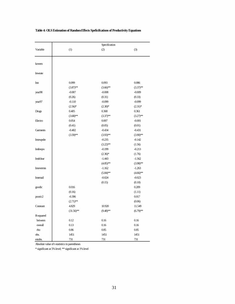
So, it is also useful to introduce the bottleneck variables into a reduced form

productivity equation (table 4). In column 2 we do this without the dummy variables for

states. Now, all five bottlenecks have coefficients with the intuitive sign and statistical

significance at the 1% level. Without the bottleneck variables, the productivity difference

between poor climate states and good climate ones in column 1 is 42 percent. (The fact

that the labor productivity difference is more than 40 points whereas the TFP difference

was 26 points confirms that capital and high-quality labor tend to migrate to the good

policy states.) If we include both dummy variables for type of state and the bottleneck

variables (column 3), the gap is no longer statistically significant. The point estimates

suggest that the better power supply in good-climate states accounts for 3 points of

21

productivity difference; fewer government visits, 3 points; and better connectivity 4

points.

7. Conclusion

It is clear from our data that the investment climate varies significantly across

India’s states. Business managers rate the investment climates of Uttar Pradesh, West

Bengal and Kerala as relatively ‘poor’, those of Maharashtra, Gujarat, Andra Pradesh,

Karnataka and Tamil Nadu as relatively ‘good’, with the states of Punjab and Delhi

somewhere in between. Although the ratings are subjective, they are also clearly driving

the investment decisions of managers. Controlling for initial capital stock, initial capital

intensity, initial debt to equity ratio, and sector of activity, the average rate of annual net

fixed capital formation is four times larger for businesses sampled from the good-climate

states.

The ratings are also broadly realistic, as regional patterns in firm productivity

show. Thus, we find that value added per worker is 45 percent lower in poor-climate

states than in good-climate states. Despite the fact that investment rates are several times

higher in good-states this gap does not seem have anything to do with differences in

capital per worker. On the other hand, approximately one-third of the gap is due to good-

climate states producing or attracting better quality workers. The balance of the gap in

labor productivity reflects lower TFP in poor-climate states.

We trace the TFP gap itself to regional differences in such objective indicators of

investment climate as the reliability of the power supply, the ease of connectivity to the

internet, the frequency of government visits to factories, the efficiency of customs

22

administration, and the rigidity of labor market regulations. Less reliable power supply

and inferior internet connectivity in poor-climate states account for more than a quarter of

the TFP differences. More than a tenth of the differences reflect greater regulatory burden

in the same states. The TFP disadvantage of poor-climate states would have been even

higher if labor market rigidity had not been more of a drag on productivity in good-

climate states.

These point estimates need to be taken with some caution, given the ambiguity of

the meaning of coefficients of proxies and the real possibility of omitted-variable biases.

They nevertheless provide a broad indication of the large gains in productivity and

investment that could be achieved in Indian states by improving regulation of firms and

the regulatory environment for infrastructure provision. Overall, this work shows the

importance of complementing India's national level policies -- a stable macro

environment and growing openness to foreign trade and investment -- with good

institutions and policies at a more local level so that efficient investment is attracted and

jobs created. A natural next step in this research is to link the variations in the investment

climate to differences in employment creation and poverty reduction across Indian states.

23

Appendix A: Sample Design of FACS-India

The seven manufacturing industries covered in the FACS of India account for about 40%

of aggregate manufacturing value added in India and over half of manufactured exports.

The focus on exporting industries arose from the survey objective of linking local

investment climates to the international competitiveness of producers. The selection of

states was based on three principles. The first was that the sample would represent states

at different levels of development, as measured by per capita GSP. The second was that

states whose investment climates were perceived to be better as indicated by, for

example, share in foreign direct investment (FDI) flows should be covered as well as

those whose economic environment was not thought to be as friendly to business. The

third principle was that each survey state would have a significant number of producers in

at least three of the industries on which the survey was intended to focus.

Of the ten states covered by the survey Delhi, Gujarat, Maharashtra, Punjab and West

Bengal are high-income states according to a recent classification by the World Bank

(1999). Uttar Pradesh is a low-income states. Andhra Pradesh, Karnataka, Kerala and

Tamil Nadu are middle-income states. Six of the 10 states attracted practically all of the

FDI flows to India in 1997-98, which we think is a measure of the contrast of their

investment climate with that of the other four, at least as perceived by the business

community at the time.

24

Our sample frame was drawn from the 1998 edition of the Kompass database for India.

This listed 67,000 businesses, from which we excluded establishments employing less

than 20 workers. This and the restriction on lines of activity and states of location led to

an effective sampling frame of 6074. The intended sample size was 1200, of which 48

were allocated to the auto components and machine tools industries for purposive

sampling towards an international benchmarking exercise. The balance was allocated

among the other six industries roughly in proportion to shares in India’s manufacturing

and service exports. Each industry sub-sample was randomly selected according to a rule

in which an establishment’s probability of selection was higher the higher was its

employment size.

25

References

Ahluwalia, I. J. 1995. India: Industrial development review. Vienna: UNIDO.

Ahluwalia, M.S. 2002. “Economic Reforms in India Since 1991: Has GradualismWorked?” Mimeo. International Monetary Fund, Washington, D.C.

Aschauer, D.A. 1989. “Is Public Expenditure Productive?” Journal of MonetaryEconomics, 23(2), 177-200.

Barro, R.J. and X. Sala-I-Martin. 1995. Economic Growth. New York: McGraw-Hill

Bils, M. and P. J. Klenow. 1998. “Does Schooling Cause Growth or the Other wayAround?” NBER Working Paper No. 6393.

Brendt, E.R. and B. Hansson. 1992. “Measuring the Contribution of Public InfrastructureCapital in Sweden.” Scandinavian Journal of Economics, Supplement, 94, S151-72.

Dollar, David and Aart Kraay, 2001, “Trade, Growth, and Poverty,” Policy ResearchWorking Paper No. 2199, World Bank, Washington, D.C.

Hall, R. and C.I. Jones. 1999. “Why Do Some Countries Produce So Much More OutputPer Worker Than Others?” Quarterly Journal of Economics , CXIV, 83-116.

Holtz-Eakin, D. 1994. “Public Sector Capital and the Productivity Puzzle.” Review ofEconomics and Statisitcs, 76 (1), 12-21

Easterly, W. and S. Rebelo. 1993. “Fiscal Policy and Economic Growth: An EmpiricalInvestigation.” Journal of Monetary Economics 32(3), 417-58.

Mincer, J. 1974. Schooling, Experience and Earnings. New York: Columbia UniversityPress.

Morrison, C.J. and A. E. Schwartz. 1996. “State Infrastruture and ProductivePefromance,” American Economic Review, December, 1095-1111.

Nadiri, M. I and T.P. Mamuneas. 1994. “Infrastructure and Public R & D Investments,and the Growth of Factor Productivity in US Manufacturing Industries.” NBERWorking Paper No. 4845.

Reinikka, R. and J. Svensson. 1999. “How Inadequate Provision of Public Infrastructureand Services Affects Private Investment.” World Bank Policy Research WorkingPaper No. 2262.

26

Sachs, J. D., A. Varshney and N. Bajpai (eds). 1999. India in the Era of EconomicReforms. New Delhi: Oxford University Press.

The World Bank. 1999. India: Reducing Poverty, Accelerating Development. New Delhi:Oxford University Press.

Zagha, R. 1999. “Labour and India’s Economic Reforms.” In Sachs et al (eds) India inthe Era of Economic Reforms. New Delhi: Oxford University Press.

27

Figure 1. Investment climate:perception of firms outside the state

UttarPradesh80

60

40

20

0

20

40

60

80Percent of respondents

BetterBest

WorseWorst

Delhi

Kerala

AndhraPradesh

GujaratKarnatakaMaharashtra

PunjabTamilNadu

WestBengal

-20

-10

10

-100 -50 50 100

% ranking better-% ranking worse

Net%

cost

savin

gby

mov

ing

to...

Maha

GujaratAP

Karna

TN

DelhiPunjab

KeralaWB

UP

Figure 2. Rankings of investment climate

28

-0.04

-0.02

0.00

0.02

0.04

0.06

0.08

0.10

Figure 3. Inter-state gaps in mean rate of netfixed investment

UttarPradesh West

Bengal

Kerala

PunjabDelhi

TamilNadu

Karnataka AndhraPradesh

Gujarat Maharashtra

29

Table 1: Notation

Notation Variable

yovern log annual value added per worker in 000 Rs.kovern log of net book value of plant and equipment per worker in 000 Rs.lnwrate log annual wage bill per worker in '000 Rseovern log annual energy bill per worker in '000 Rslnn log of number of employees at the end of the yearGarments dummy=1 for business in the garments industryDrugs dummy=1 for business in the pharmaceuticals industrElectrog dummy=1 for producers of electronics or of electrical white goodsmowpshr state level mean of percentage share of power supply from own generatorsmfreqvis state level mean of annual number of regulatory visits by government officialsmdclear state level mean of number of days it took the last consignment of imports to clear customsmoverman state level mean of reported percentage of overmanningmemail state level proportion of establishments that use the internet to communicate with customers

Table 2: Descriptive Statistics

All Good-climate states Medium-climate states Poor-climate statesVariables Mean Std. Dev Mean Std. Dev Mean Std. Dev Mean Std. Devyovern 5.19 1.19 5.29 1.21 5.12 1.19 4.84 0.99kovern 5.12 1.54 5.26 1.50 4.92 1.70 4.74 1.36eovern 2.60 1.45 2.66 1.52 2.42 1.40 2.61 1.14lnwrate 3.63 0.98 3.68 1.04 3.63 0.87 3.40 0.82lnn 4.17 1.62 4.42 1.64 3.78 1.54 3.56 1.40mowpshr 25.68 9.04 22.55 4.91 30.93 2.63 31.92 18.88moverman 16.94 8.76 18.02 10.38 15.33 0.47 14.47 6.43mfreqvis 10.78 14.35 8.19 2.56 17.03 28.85 12.68 1.68mdclear 8.27 2.47 8.37 1.98 6.71 0.71 10.51 4.15memail 0.45 0.14 0.44 0.14 0.59 0.05 0.31 0.06Drugs 0.28 0.45 0.29 0.45 0.16 0.37 0.44 0.50Electro 0.15 0.36 0.15 0.36 0.22 0.41 0.03 0.17Garments 0.27 0.45 0.24 0.43 0.34 0.47 0.31 0.46

Obs. 1451 931 328 192

30

Table 3: GLS Estimation of Random Effects Speficifcations of Productivity Equations***Dependent variable =log of value added per worker

SpecificationVariable (1) (2) (3) (4)

kovern 0.375 0.381 0.402 0.409(9.27)** (9.45)** (9.89)** (10.00)**

lnwrate 0.628 0.620 0.606 0.603(20.74)** (20.47)** (19.96)** (19.79)**

lnn 0.048 0.039 0.028 0.026(2.79)** (2.22)* (1.61) (1.46)

year98 0.042 0.041 0.040 0.040(1.70) (1.67) (1.64) (1.62)

year97 0.051 0.052 0.050 0.049(1.27) (1.30) (1.25) (1.22)

Drugs 0.225 0.251 0.253 0.237(3.03)** (3.38)** (3.39)** (3.16)**

Electro -0.024 -0.048 -0.077 -0.085(0.27) (0.53) (0.86) (0.96)

Garments -0.082 -0.077 -0.084 -0.088(1.07) (1.01) (1.10) (1.15)

goodic 0.0002 0.214(0.00) (1.67)

pooric2 -0.2599 0.287(2.63)** (1.50)

lmdclear -0.594 -0.883(2.91)** (3.28)**

lmemail 0.299 0.449(2.68)** (2.97)**

lmfreqvs -0.085 -0.176(1.48) (2.14)*

lmovermn -0.416 -0.626(3.03)** (3.36)**

lmowpshr -0.192 -0.148(3.85)** (2.38)*

Constant 0.729 0.792 3.167 4.561(3.68)** (3.92)** (3.85)** (3.88)**

R-squaredbetween 0.59 0.60 0.61 0.61overall 0.56 0.60 0.58 0.58rho 0.74 0.73 0.73 0.73

Observations 1451 1451 1451 1451Number of estbs. 731 731 731 731Absolute value of t-statistics in parentheses* significant at 5% level; ** significant at 1% level

*** Capital services instrumented by energy consumption

31

Table 4: OLSEstimationof RandomEffects Speficifcations of Productivity Equations

Specification

Variable (1) (2) (3)

kovern

lnwrate

lnn 0.099 0.093 0.086

(3.87)** (3.66)** (3.37)**

year98 -0.007 -0.008 -0.009

(0.26) (0.31) (0.33)

year97 -0.110 -0.099 -0.099

(2.56)* (2.30)* (2.31)*

Drugs 0.405 0.368 0.361

(3.68)** (3.37)** (3.27)**

Electro 0.054 0.007 -0.001

(0.41) (0.05) (0.01)

Garments -0.402 -0.434 -0.431

(3.59)** (3.93)** (3.90)**

lmowpshr -0.235 -0.142

(3.22)** (1.56)

lmfreqvs -0.199 -0.213

(2.36)* (1.76)

lmdclear -1.443 -1.562

(4.85)** (3.98)**

lmovermn -1.162 -1.263

(5.84)** (4.66)**

lmemail -0.024 -0.023

(0.15) (0.10)

goodic 0.016 0.209

(0.16) (1.11)

pooric2 -0.396 0.017

(2.71)** (0.06)

Constant 4.829 10.920 11.549

(31.56)** (9.48)** (6.79)**

R-squared

between 0.12 0.16 0.16

overall 0.13 0.16 0.16

rho 0.86 0.85 0.85

obs. 1451 1451 1451

estabs. 731 731 731

Absolute value of t-statistics in parentheses

* significant at 5%level; ** significant at 1%level

32

Table 5: Proportionate Regional Gap in value added per worker vis-à-vis medium climate states

Gap in value added Gap in value added due to differences inRegions capital aveage skill TFP

per worker levelsGood-climate 0.1760 0.0525 0.03493752 0.0002

Poor-climate -0.2746 0.04125 -0.1395881 -0.2599

Table 6: Effects of Indicators of Investment Climate on TFP

Regions Proportinate gap in value added vis-à-vis medium-climate states due tomowpshr memail mdclear mfreqvs movermn

Good-climate 0.0263288 -0.0391536 -0.057014 0.02702457 -0.0291956

Poor-climate -0.0026445 -0.0823962 -0.1158723 0.01089048 0.01040331