Working Paper #13003: Longitudinal Design Options for the Medical
27
ARTICLE Communicated by Roger Brockett Estimating a State-Space Model from Point Process Observations Anne C. Smith [email protected] Neuroscience Statistics Research Laboratory, Department of Anesthesia and Critical Care, Massachusetts General Hospital, Boston, MA 02114, U.S.A. Emery N. Brown [email protected] Neuroscience Statistics Research Laboratory, Department of Anesthesia and Critical Care, Massachusetts General Hospital, Boston, MA 02114, U.S.A., and Division of Health Sciences and Technology, Harvard Medical School/Massachusetts Institute of Technology, Cambridge, MA 02139, U.S.A. A widely used signal processing paradigm is the state-space model. The state-space model is de ned by two equations: an observation equation that describes how the hidden state or latent process is observed and a state equation that de nes the evolution of the process through time. In- spired by neurophysiology experiments in which neural spiking activity is induced by an implicit (latent) stimulus, we develop an algorithm to estimate a state-space model observed through point process measure- ments. We represent the latent process modulating the neural spiking activity as a gaussian autoregressive model driven by an external stim- ulus. Given the latent process, neural spiking activity is characterized as a general point process de ned by its conditional intensity function. We develop an approximate expectation-maximization (EM) algorithm to estimate the unobservable state-space process, its parameters, and the pa- rameters of the point process. The EM algorithm combines a point process recursive nonlinear lter algorithm, the xed interval smoothing algo- rithm, and the state-space covariance algorithm to compute the complete data log likelihood ef ciently. We use a Kolmogorov-Smirnov test based on the time-rescaling theorem to evaluate agreement between the model and point process data. We illustrate the model with two simulated data examples: an ensemble of Poisson neurons driven by a common stimulus and a single neuron whose conditional intensity function is approximated as a local Bernoulli process. Neural Computation 15, 965–991 (2003) c ° 2003 Massachusetts Institute of Technology
Transcript of Working Paper #13003: Longitudinal Design Options for the Medical
ARTICLE Communicated by Roger Brockett
Estimating a State-Space Model from Point ProcessObservations
Anne C SmithasmithneurostatmghharvardeduNeuroscience Statistics Research Laboratory Department of Anesthesia and CriticalCare Massachusetts General Hospital Boston MA 02114 USA
Emery N BrownbrownneurostatmghharvardeduNeuroscience Statistics Research Laboratory Department of Anesthesia and CriticalCare Massachusetts General Hospital Boston MA 02114 USA and Division ofHealth Sciences and Technology Harvard Medical SchoolMassachusetts Institute ofTechnology Cambridge MA 02139 USA
A widely used signal processing paradigm is the state-space model Thestate-space model is dened by two equations an observation equationthat describes how the hidden state or latent process is observed and astate equation that denes the evolution of the process through time In-spired by neurophysiology experiments in which neural spiking activityis induced by an implicit (latent) stimulus we develop an algorithm toestimate a state-space model observed through point process measure-ments We represent the latent process modulating the neural spikingactivity as a gaussian autoregressive model driven by an external stim-ulus Given the latent process neural spiking activity is characterizedas a general point process dened by its conditional intensity functionWe develop an approximate expectation-maximization (EM) algorithm toestimate the unobservable state-space process its parameters and the pa-rameters of the point process The EM algorithm combines a point processrecursive nonlinear lter algorithm the xed interval smoothing algo-rithm and the state-space covariance algorithm to compute the completedata log likelihood efciently We use a Kolmogorov-Smirnov test basedon the time-rescaling theorem to evaluate agreement between the modeland point process data We illustrate the model with two simulated dataexamples an ensemble of Poisson neurons driven by a common stimulusand a single neuron whose conditional intensity function is approximatedas a local Bernoulli process
Neural Computation 15 965ndash991 (2003) cdeg 2003 Massachusetts Institute of Technology
966 A Smith and E Brown
1 Introduction
A widely used signal processing paradigm in many elds of science andengineering is the state-space model The state-space model is dened bytwo equations an observation equation that denes what is being mea-sured or observed and a state equation that denes the evolution of theprocess through time State-space models also termed latent process mod-els or hidden Markov models have been used extensively in the analysis ofcontinuous-valued data For a linear gaussian observation process and alinear gaussian state equation with known parameters the state-space esti-mation problem is solved using the well-known Kalman lter Many exten-sions of this algorithm to both nongaussian nonlinear state equations andnongaussian nonlinear observation processes have been studied (Ljung ampSoderstrom 1987 Kay 1988 Kitagawa amp Gersh 1996 Roweis amp Ghahra-mani 1999 Gharamani 2001) An extension that has received less attentionand the one we study here is the case in which the observation model is apoint process
This work is motivated by a data analysis problem that arises from aform of the stimulus-response experiments used in neurophysiology In thestimulus-response experiment a stimulus under the control of the exper-imenter is applied and the response of the neural system typically theneural spiking activity is recorded In many experiments the stimulus isexplicit such as the position of a rat in its environment for hippocampalplace cells (OrsquoKeefe amp Dostrovsky 1971 Wilson amp McNaughton 1993) ve-locity of a moving object in the visual eld of a y H1 neuron (Bialek Riekede Ruyter van Steveninck amp Warland 1991) or light stimulation for retinalganglion cells (Berry Warland amp Meister 1997) In other experiments thestimulus is implicit such as for a monkey executing a behavioral task inresponse to visual cues (Riehle Grun Diesmann amp Aertsen 1997) or traceconditioning in the rabbit (McEchron Weible amp Disterhoft 2001) The neu-ral spiking activity in implicit stimulus experiments is frequently analyzedby binning the spikes and plotting the peristimulus time histogram (PSTH)When several neurons are recorded in parallel cross-correlations or unitaryevents analysis (Riehle et al 1997 Grun Diesmann Grammont Riehle ampAertsen 1999) have been used to analyze synchrony and changes in ringrates Parametric model-based statistical analysis has been performed forthe explicit stimuli of hippocampal place cells using position data (BrownFrank Tang Quirk amp Wilson 1998) However specifying a model when thestimulus is latent or implicit is more challenging State-space models sug-gest an approach to developing a model-based framework for analyzingstimulus-response experiments when the stimulus is implicit
We develop an approach to estimating state-space models observedthrough a point process We represent the latent (implicit) process modulat-ing the neural spiking activity as a gaussian autoregressive model drivenby an external stimulus Given the latent process neural spiking activity
State Estimation from Point Process Observations 967
is characterized as a general point process dened by its conditional inten-sity function We will be concerned here with estimating the unobservablestate or latent process its parameters and the parameters of the point pro-cess model Several approaches have been taken to the problem of simul-taneous state estimation and model parameter estimation the latter beingtermed system identication (Roweis amp Ghahramani 1999) In this article wepresent an approximate expectation-maximization (EM) algorithm (Demp-ster Laird amp Rubin 1977) to solve this simultaneous estimation problemThe approximate EM algorithm combines a point process recursive nonlin-ear lter algorithm the xed interval smoothing algorithm and the state-space covariance algorithm to compute the complete data log likelihoodefciently We use a Kolmogorov-Smirnov test based on the time-rescalingtheorem to evaluate agreement between the model and point process dataWe illustrate the algorithm with two simulated data examples an ensem-ble of Poisson neurons driven by a common stimulus and a single neuronwhose conditional intensity function is approximated as a local Bernoulliprocess
2 Theory
21 Notation and the Point Process Conditional Intensity FunctionLet 0 T] be an observation interval during which we record the spikingactivity of C neurons Let 0 lt uc1 lt uc2 lt lt ucJc
middot T be the set of Jcspike times (point process observations) from neuron c for c D 1 C Fort 2 0 T] let Nc
0t be the sample path of the spike times from neuron c in 0 t]It is dened as the event Nc
0t D f0 lt uc1 lt uc2 ucj middot tT
Nct D jgwhere Nct is the number of spikes in 0 t] and j middot Jc The sample path isa right continuous function that jumps 1 at the spike times and is constantotherwise (Snyder amp Miller 1991) This function tracks the location andnumber of spikes in 0 t] and therefore contains all the information in thesequence of spike times Let N0t D fN1
0t NC0tg be the ensemble spiking
activity in 0 t]The spiking activity of each neuron can depend on the history of the
ensemble as well as that of the stimulus To represent this dependence wedene the set of stimuli applied in 0 t] as S0t D f0 lt s1 lt lt s` middot tgLet Ht D fN0t S0tg be the history of all C neurons up to and including timet To dene a probability model for the neural spiking activity we dene theconditional intensity function for t 2 0 T] as (Cox amp Isham 1980 Daley ampVere-Jones 1988)
cedilct j Ht D lim10
PrNc0tC1
iexcl Nc0t D 1 j Ht
1 (21)
The conditional intensity function is a history-dependent rate function thatgeneralizes the denition of the Poisson rate (Cox amp Isham 1980 Daley amp
968 A Smith and E Brown
Vere-Jones 1988) If the point process is an inhomogeneous Poisson pro-cess the conditional intensity function is cedilct j Ht D cedilct It follows thatcedilct j Ht1 is the probability of a spike in [t t C 1 when there is historydependence in the spike train In survival analysis the conditional inten-sity is termed the hazard function because in this case cedilct j Ht1 measuresthe probability of a failure or death in [t t C 1 given that the process hassurvived up to time t (Kalbeisch amp Prentice 1980)
22 Latent Process Model Sample Path Probability Density and theComplete Data Likelihood It is possible to dene the latent process in con-tinuous time However to simplify the notation for our ltering smoothingand EM algorithms we assume that the latent process is dened on a dis-crete set of evenly spaced lattice points To dene the lattice we choose Klarge and divide 0 T] into K intervals of equal width 1 D T=K so that thereis at most one spike per interval The latent process model is evaluated atk1 for k D 1 K We also assume the stimulus inputs can be measuredat a resolution of 1
We dene the latent model as the rst-order autoregressive model
xk D frac12xkiexcl1 C regIk C k (22)
where xk is the unknown state at time k1 frac12 is a correlation coefcientIk is the indicator function that is 1 if there is a stimulus at k1 and zerootherwise reg modulates the effect of the stimulus on the latent process andk is a gaussian random variable with mean zero and variance frac34 2
Whilemore complex latent process models can certainly be dened equation 22is adequate to illustrate the essential features of our algorithm
The joint probability density of the latent process is
px j frac12 reg frac34 2 D
micro1 iexcl frac122
2frac14frac34 2
para 12
pound exp
(iexcl 1
2
1 iexcl frac122
frac34 2
x20
CKX
kD1
xk iexcl frac12xkiexcl1 iexcl regIk2
frac34 2
) (23)
where x D x0 x1 xKWe assume that the conditional intensity function is cedilck1 j xk Hc
k microcurrenc
where microcurrenc is an unknown parameter We can express the joint probability
density of the sample path of neuron c conditional on the latent process as(Barbieri Quirk Frank Wilson amp Brown 2001 Brown Barbieri Ventura
State Estimation from Point Process Observations 969
Kass amp Frank 2002)
pNc0T j x Hc
T micro currenc D exp
Z T
0log cedilcu j xu Hc
u micro currenc dNcu
iexclZ T
0cedilcu j xu Hc
u microcurrenc du
(24)
where dNcu D 1 if there is a spike at u from neuron c and 0 otherwiseUnder the assumption that the neurons in the ensemble are conditionallyindependent given the latent process the joint probability density of thesample paths of the ensemble is
pN0T j x HT micro curren DCY
cD1
pNc0T j x Hc
T micro currenc (25)
where micro curren D micro curren1 micro curren
C
23 Parameter Estimation Expectation-Maximization Algorithm Toillustrate the algorithm we choose a simple form of the conditional inten-sity function That is we take the conditional intensity function for neuronc as
cedilck1 D expsup1c C macrcxk (26)
where sup1c is the log of the background ring rate and macrc is its gain parameterthat governs how much the latent process modulates the ring rate of thisneuron Here we have micro curren
c D sup1c macrc Equations 23 and 26 dene a doublystochastic point process (Cox amp Isham 1980) If we condition on the latentprocess then equation 26 denes an inhomogeneous Poisson process Un-der this model all the history dependence is through the stimulus We letmicro D frac12 reg frac34 2
microcurren Because our objective is to estimate the latent process xand to compute the maximum likelihood estimate of the model parametermicro we develop an EM algorithm (Dempster et al 1977) In our EM algo-rithm we treat the latent process x as the missing or unobserved quantityThe EM algorithm requires us to maximize the expectation of the completedata log likelihood It follows from equations 23 and 26 that the completedata likelihood for our model is
pN0T x j micro D pN0T j x microcurrenpx j frac12 reg frac34 2 (27)
231 E-Step At iteration`C1 of the algorithm we compute in the E-stepthe expectation of the complete data log likelihood given HK the ensemble
970 A Smith and E Brown
spiking activity and stimulus activity in 0 T] and micro ` the parameter esti-mate from iteration ` By our notation convention in the previous sectionsince K1 D T HK D HT and
Qmicro j micro ` D E[log[pN0T x j micro] k HK micro `]
D E
KX
kD0
CX
cD1dNck1sup1c C macrcxk C log 1
iexcl expsup1c C macrcxk1 k HK micro `
C E
KX
kD1
iexcl 12
xk iexcl frac12xkiexcl1 iexcl regIk2
frac34 2
iexcl K2
log 2frac14 iexcl K2
log frac34 2 k HK micro `
C E
12
log1 iexcl frac122 iexcl 12
x201 iexcl frac122
frac34 2
k HK micro `
(28)
Upon expanding the right side of equation 28 we see that calculating theexpected value of the complete data log likelihood requires computing theexpected value of the latent process E[xk k HK micro `] and the covariancesE[x2
k k HK micro `] and E[xkxkC1 k HK micro `] We denote them as
xkjK acute E[xk k HK micro `] (29)
Wk acute E[x2k k HK micro `] (210)
WkkC1 acute E[xkxkC1 k HK micro `] (211)
for k D 1 K where the notation k j j denotes the expectation of thelatent process at k1 given the ensemble spiking activity and the stimu-lus up to time j1 To compute these quantities efciently we decomposethe E-step into three parts a forward nonlinear recursive lter to computexkjk a backward xed interval smoothing (FIS) algorithm to estimate xkjKand a state-space covariance algorithm to estimate Wk and WkkC1 This ap-proach for evaluating the complete data log likelihood was suggested rstby Shumway and Stoffer (1982) They used the FIS but a more complicatedform of the state-covariance algorithm An alternative covariance algorithmwas given in Brown (1987) The logic of this approach is to compute the for-ward mean and covariance estimates and combine them with the backwardmean and covariance estimates to obtain equations 210 and 211 This ap-proach is exact for linear gaussian latent process models and linear gaussian
State Estimation from Point Process Observations 971
observation processes For our model it will be approximate because ourobservations form a point process
E-Step I Nonlinear Recursive Filter The following equations comprise arecursive nonlinear ltering algorithm to estimate xkjk and frac34 2
kjk using equa-tion 26 as the conditional intensity The algorithm is based on the maximuma posterori derivation of the Kalman lter algorithm (Mendel 1995 Brownet al 1998) It recursively computes a gaussian approximation to the pos-terior probability density pxk j Hk micro ` The approximation is based onrecursively computing the posterior mode xkjk and computing its variancefrac34 2
kjk as the negative inverse of the second derivative of the log posteriorprobability density (Tanner 1996) The nonlinear recursive algorithm is
(Observation Equation)
pdNk1 j xk DCY
cD1
[expsup1c C macrcxk1]dNck1
pound expiexcl expsup1c C macrcxk1 (212)
(One-Step Prediction)
xkjkiexcl1 D frac12xkiexcl1jkiexcl1 C regIk (213)
(One-Step Prediction Variance)
frac34 2kjkiexcl1 D frac122frac34 2
kiexcl1jkiexcl1 C frac34 2 (214)
(Posterior Mode)
xkjk D xkjkiexcl1 C frac34 2kjkiexcl1
CX
cD1
macrc[dNck1 iexcl expsup1c C macrcxkjk1] (215)
(Posterior Variance)
frac34 2kjk D iexcl
iexclfrac34 2
kjkiexcl1iexcl1 iexclCX
iD1
macr2c expsup1c C macrcxkjk1
iexcl1
(216)
for k D 1 K The initial condition is x0 and frac34 20j0 D frac34 2
1 iexcl frac122iexcl1 Thealgorithm is nonlinear because xkjk appears on the left and right of equa-tion 215 The derivation of this algorithm for an arbitrary point processmodel is given in the appendix
E-Step II Fixed Interval Smoothing (FIS) Algorithm Given the sequence ofposterior mode estimates xkjk (see equation 215) and the variance frac34 2
kjk (see
972 A Smith and E Brown
equation 216) we use the xed interval smoothing algorithm to computexkjK and frac34 2
kjK The algorithm is (Mendel 1995 Brown et al 1998)
xkjK D xkjk C AkxkC1jK iexcl xkC1jk (217)
where
Ak D frac12frac34 2kjkfrac34
2kC1jk
iexcl1 (218)
and
frac34 2kjK D frac34 2
kjk C A2kfrac34 2
kC1jK iexcl frac34 2kC1jk (219)
for k D K iexcl 1 1 and initial conditions xKjK and frac34 2KjK
E-Step III State-SpaceCovariance Algorithm The covarianceestimate frac34kujKcan be computed from the state-space covariance algorithm (de Jong ampMacKinnon 1988) and is given as
frac34kujK D Akfrac34kC1ujK (220)
for 1 middot k middot u middot K It follows that the covariance terms required for theE-step are
WkkC1 D frac34kkC1jK C xkjKxkC1jK (221)
and
Wk D frac34 2kjK C x2
kjK (222)
232 M-Step In the M-step we maximize the expected value of thecomplete data log likelihood in equation 28 with respect to micro `C1 In sodoing we obtain the following closed-form solutions for frac12`C1 reg`C1 andfrac34
2`C1
frac12`C1
reg`C1
D
2
66664
KX
kD1
Wkiexcl1
KX
kD1
xkiexcl1jkIk
KX
kD1
xkiexcl1jkIk
KX
kD1
Ik
3
77775
iexcl1 2
66664
KX
kD1
Wkkiexcl1
KX
kD1
xkjkIk
3
77775(223)
frac34 2`C1 D Kiexcl1
KX
kD1
Wk C frac122`C1KX
kD1
Wkiexcl1 C reg2`C1KX
kD1
Ik
State Estimation from Point Process Observations 973
iexcl 2frac12`C1KX
kD1
Wkkiexcl1iexcl2reg`C1KX
kD1
xkjKIkC2frac12`C1reg`C1
poundKX
kD1
xkiexcl1jKIk C W0
plusmn1 iexcl frac122`C1
sup2
(224)
where initial conditions for the latent process are estimated from x`C10 D
frac12`C1x1jK and frac342`C10j0 D frac34
2`C1 1 iexcl frac122`C1iexcl1 The closed-form solution for
frac12`C1 in equation 223 is obtained by neglecting the last two terms in theexpectation of the complete data log likelihood (see equation 28) This ap-proximation means that we estimate frac12`C1 from the probability density ofx1 xK given x0 and the point processmeasurements instead of the proba-bility density of x0 xK given the point process measurements Inclusionof the last two terms results in a cubic equation for computing frac12`C1 whichis avoided by using the closed-form approximation We report only the re-sults of the closed-form solution in section 3 because we found that for ouralgorithms the absolute value of the fractional difference between the twosolutions was less than 10iexcl6 (ie jcubic solution-closed form solutionj=cubicsolution lt 10iexcl6)
The parameter sup1`C1c is estimated as
sup1`C1c D log NcT
iexcl log
AacuteKX
kD1
expsup3
macr`C1c xkjK C
12
macr2`C1c frac34 2
kjK
acute1
(225)
whereas macr`C1c is the solution to the nonlinear equation
KX
kD1
dNck1xkjK
D exp sup1`C1c
(KX
kD1
expsup3
macr`C1c xkjK C
12
macr`C1c frac34 2
kjK
acute
pound xkjK C macr`C1c frac34 2
kjK1
)
(226)
which is solved by Newtonrsquos method after substituting sup1`C1c from equa-
tion 226 The expectations needed to derive equations 225 and 226 werecomputed using the lognormal probability density and the approximationof pxk j HK micro ` as a gaussian probability density with mean xkjK andvariance frac34 2
kjK
974 A Smith and E Brown
24 Assessing Model Goodness-of-Fit by the Time-Rescaling Theo-rem The latent process and point process models along with the EM al-gorithm provide a model and an estimation procedure for computing thelatent process and the parameter vector micro It is important to evaluate modelgoodness-of-t that is determine how well the model describes the neu-ral spike train data series data Because the spike train models are denedin terms of an explicit point process model we can use the time-rescalingtheorem to evaluate model goodness-of-t To do this we compute for eachneuron the time-rescaled or transformed interspike intervals
iquestj DZ uj
ujiexcl1
cedilu j Omicro du (227)
where the ujs are the spike times from the neuron and cedilt j micro is the condi-tional intensity function in equation 26 evaluated at the maximum likeli-hood estimate Omicro for j D 1 J where we have dropped the subscript c tosimplifynotation The ujs are a point process with a well-dened conditionalintensity function and hence by the time-rescaling theorem the iquestjs are inde-pendent exponential random variables with a unit rate (Barbieri et al 2001Brown et al 2002) Under the further transformation zj D 1iexclexpiexcliquestj the zjsare independent uniform random variables on the interval (01) Thereforewe can construct a Kolmogorov-Smirnov (K-S) test to measure agreementbetween the zjs and the uniform probability density (Barbieri et al 2001Brown et al 2002) First we order the zjs from the smallest to the largestvalue Then we plot values of the cumulative distribution function of the
uniform density dened as bj D jiexcl 12
J for j D 1 J against the ordered zjsThe points should lie on the 45 degree line Because the transformation fromthe ujs to the zjs is one-to-one a close agreement between the probabilitydensity of the zjs and the uniform probability density on (01) indicates closeagreement between the (latent process-point process) model and the pointprocess measurements Hence the time-rescaling theorem provides a directmeans of measuring agreement between a point process or neural spiketrain time series and a probability model intended to describe its stochasticstructure
3 Applications
31 Example 1 Multiple Neurons Driven by a Common Latent ProcessTo illustrate our analysis paradigm we simulate C D 20 simultaneouslyrecorded neurons from the model described by equations 22 and 26 Thetime interval for the simulation was T D 10 seconds and the latent processmodel parameters were frac12 D 099 reg D 3 and frac34 2
D 10iexcl3 with the implicitstimulus Ik applied at 1 second intervals The parameters for the conditionalintensity function dening the observation process were the log of the back-ground ring rate sup1 D iexcl49 for all neurons whereas the gain coefcients
State Estimation from Point Process Observations 975
Table 1 True Parameter Values and EM Algorithm Parameter Estimates
Parameter True Estimate Parameter True Estimate
frac12 0990 0993 macr10 1079 1190reg 3000 2625 macr11 1008 1039sup1 iexcl4900 iexcl5105 macr12 1078 1247macr1 1075 1261 macr13 1009 1031macr2 0989 1060 macr14 1078 1129macr3 1035 1039 macr15 0980 1121macr4 0973 1101 macr16 0976 1164macr5 1003 1190 macr17 0990 1234macr6 0992 1132 macr18 0968 1154macr7 0977 1118 macr19 0956 0979macr8 1027 1176 macr20 1098 1350macr9 1066 1089
macrc for the 20 neurons were chosen randomly on the interval [09 11] Theseparameter values for the latent and observation processes were chosen togive an approximate average ring rate of 10 Hz for each neuron The neu-ral spike trains were simulated using the time-rescaling theorem algorithmdescribed in Brown et al (2002) and the state equations in the EM algorithmwere updated at 1 D 1 msec
Using the EM algorithm described in the previous section we t themodel in equations 22 and 26 simultaneously to the 20 simulated neuralspike trains assuming a xed noise variance frac34 2
D 10iexcl3 The convergencecriteria for the algorithm were absolute changes of less than 10iexcl2 in consecu-tive iterates of the parameters and relative changes in the parameter iteratesof less than 10iexcl3 that is jold iexcl newj=old lt 10iexcl3 The parameter estimatesfrom the EM algorithm were in good agreement with the true values usedto simulate the spike train data (see Table 1) In this case the overestimatesof the gain coefcients macrc are offset by the underestimates of reg and sup1
Approximating the probability density of the state at k1 as the gaussiandensity with mean Oxk and variance Ofrac34 2
k it follows from equation 26 andthe standard change of variables formula from probability theory that theprobability density of the rate for neuron c at time k1 is the lognormalprobability density dened as
pcedilck j Osup1c Oc Oxk D 2frac14 Ofrac34 2
k iexcl 12 Occedil
ck
iexcl1
pound exp
0
iexcl 12
Oiexcl1c log cedilc
k iexcl Osup1c iexcl Oxk
Ofrac34k
21
A (31)
where Osup1c and Oc are the EM algorithm estimates of sup1c and macrc for c D 1 20The 1 iexcl raquo condence limits for the rate are computed simply by using the
976 A Smith and E Brown
relation between the lognormal and standard gaussian probabilities to ndthe raquo=2 and 1 iexcl raquo=2 quantiles of the probability density in equation 31 forraquo 2 0 1 In our analyses we take raquo D 005 and construct 95 condenceintervals
To compare our model-based analysis with current practices for analyz-ing neural spike train data using empirical smoothing methods we alsoestimated the rate function for each of the 20 neurons by dividing the num-ber of spikes in a 100 msec window by 100 msec The window was thenshifted 1 msec to give the same temporal resolution as in our updating algo-rithms Because the latent process drives all the neurons we also estimatedthe population rate by averaging the rates across all 20 neurons This is acommonly used empirical temporal smoothing algorithm for computingspike rate that does not make use of stimulus information in the estima-tion (Riehle et al 1997 Grun et al 1999 Wood Dudchenko amp Eichen-baum 1999)
The condence limits of the model-based rate function give a good es-timate of the true ring rate used to generate the spikes (see Figure 1) Inparticular the estimates reproduce the magnitude and duration of the effectof the implicit stimulus on the spike ring rate The population ring rateestimated using temporal smoothing across all neurons is misleading (seeFigure 1 dot-dashed line) in that around the time of the stimuli it has di-minished amplitude and is spread out in time Furthermore if we smooth asingle spike train without averaging across neurons spurious peaks in thering rate can be produced due to noise (see Figure 1 solid gray line) Byusing information about the timing of the stimulus the model ring rateestimate follows the true rate function more closely
The 95 condence bounds for the state process estimated from the EMalgorithm cover almost completely the time course of the true state process(see Figure 2) The true state lies sometimes outside the condence limits inregions where there are very few spikes and hence little information aboutthe latent process
To assess how well the model ts the data we apply the K-S goodness-of-t tests based on the time-rescaling theorem as described in section 24(see Figure 3) In Figures 3A 3B and 3C the solid black line represents exactagreement between the model and spike data and dotted lines represent95 condence limits For 18 of 20 neurons the model lies within the con-dence limits indicating a good t to the data In contrast for 14 of the 20neurons the empirical estimate lies outside the condence limits For 6 of 20neurons both the model and empirical estimates lie within the condencelimits (see Figure 3B) In two cases the model lies outside the condencelimits (see Figure 3C) In both cases where the model does not t the datathe empirical estimate does not either Thus the model appears to give aconsiderably more accurate description of the spike train than the empiricalestimate
State Estimation from Point Process Observations 977
Figure 1 A 2000 millisecond segment of data from neuron 8 in the 20-neuronsimulation study of latent process estimation by the EM algorithm from exam-ple 1 During this period 26 spikes (verticalbarsaboveabscissa)are concentratedaround two stimulus events at 5000 msec and 6000 msec The 95 condencebands for the ring rate estimated by the latent model (dashed lines) cover thetrue rate (solid black line) used to generate the spikes most of the time In con-trast when the ring rate for neuron 8 is estimated empirically (solid gray line)using a 100 msec smoothing window (ie by dividing the number of spikes ina 100 msec window by 100 msec) the stimuli appear diminished in amplitudeand spread out in time Furthermore a spurious third peak in ring rate is pro-duced approximately 200 ms after the true rst peak This third peak is avoidedby using a smoothed estimate that is averaged over all cells (dash-dotted blackline) but the EM algorithm estimate of the ring rate based on the model moreaccurately reproduces the features of the stimuli
32 Example 2 Single Neuron Latent Stimulus-Response Model Acommon practice is to use the binomial probability mass function as a localmodel for analyzing neural spike trains We demonstrate how the parame-ters of a local Bernoulli model may be estimated using our EM algorithmWe generate a single spike train subject to multiple repeated stimuli over aperiod of approximately 1 minute In this example the conditional intensityis given by
cedilk11 D expsup1 C xk1 frac14expsup1 C xk1
1 C expsup1 C xk1D pk (32)
978 A Smith and E Brown
Figure 2 True state (solid black line) and estimated 95 condence limits(dashed lines) for the true state computed from the spike train observed inFigure 1 using the EM algorithm The estimated condence limits computed asxkjk sect 196frac34kjk fail to cover the true state when few spikes are discharged (egnear 5700 ms)
Figure 3 Facing page Kolmogorov-Smirnov goodness-of-t analyses based onthe time-rescaling theorem for three representative neurons Each panel is theK-S plots comparing the model rate estimate (dashed line) the empirical rateestimate (solid gray line) and the true rate (solid black line) In these guresthe 45 degree line in black represents an exact agreement between the modeland the spike data Dotted lines in each panel are the 95 condence limits (seeBrown et al 2002 for details) Since the true rate was used to generate spikesthe true rate KS plot always lies within the condence limits (A) An exampleof the KS plot from 1 of the 18 out of the 20 neurons for which the model-basedestimate of the KS plot was entirely within the condence limits indicating closeagreement between the overall model t and the simulated data (B) An exampleof 1 of the 6 out of the 20 neurons for which the K-S plot based on the empiricalrate estimate completely lies within the 95 condence limits (C) An exampleof 1 of the 2 out of the 20 neurons for which the K-S plot based on the modelestimate of the rate function fails to fall within the 95 condence limits Forboth of these neurons as this panel suggests the KS plot based on the empiricalrate model did not remain in the 95 condence bounds
State Estimation from Point Process Observations 979
and spikes are generated with the local Bernoulli model
pdNk1 j Hk D pdNk1k 1 iexcl pk
1iexcldNk1 (33)
with parameters sup1 D iexcl46 reg D 4 and frac12 D 08 The implicit stimulus isapplied at 40 time points We assume the noise frac34 2
in the latent process is02 In this example we set 1 D 5 msec This generates a spike train with
980 A Smith and E Brown
Table 2 True Parameter Values and the EM Algorithm Parameter Estimates
Parameter frac12 reg frac34 2 sup1
True 0800 4000 0200 iexcl4600Estimate 0804 3573 0125 iexcl4404
an average ring rate over the minute period of approximately 10 Hz Theparameters including the noise variance frac34 2
are again estimated using theEM algorithm and are in good agreement with their true values (see Table 2)
As in the previous example condence intervals were computed for thetrue rate function by deriving the probability density function for cedilk usingthe standard change of variable formula Firing rates estimated by the modelare compared with the empirical temporally smoothed rate computed bycounting spikes in a 100 msec window and then dividing by 100 msec
The ring rate (95 condence limits) computed by the model comparesfavorably with the original rate used to generate the spikes (see Figure 4)The 95 condence limits for the model estimate the magnitude and shapeof the stimulus effect on the rate even when the stimulus has little obviouseffect on the spike train This is because the estimates for each stimulusrsquoseffect are made based on the whole time series In contrast the temporallysmoothed estimate of rate does not clearly identify stimulus effects on thespike train (see Figure 4 solid gray line)The choiceof a 100 msec window forthese simulated data appears too large as increases in ringrate at the stimuliare smoothed out We can also make an overall estimate of the accuracy ofthe ring rates by comparing the model and the empirical ring rates withthe true ring at the stimulus times namely at 40 points in time wherewe applied the stimulus during the 1 minute epoch of simulated data Themean differences (standard error) between the empirical and model ratescompared to the true rate at these timesare iexcl1139 (45) Hzand iexcl85 (44) Hzrespectively Thus the model provides a signicantly better approximationto the true rate than the empirical method (Studentrsquos t-test p lt 10iexcl6) Theestimate of the state variable is found to compare well with the true stateused to generate the spike train (see Figure 5)
Again we assess model goodness-of-t using the K-S plot (see Figure 6)The t of model lies within the 95 condence limits except at very smallquantiles and follows closely the curve for the true ring rate In contrastthe t for the empirical 100 msec temporal smoothing method lies outsidethe condence limits for a large portion of the total time indicating poor tto the distribution over low and high percentiles
33 An Extension to More General Point Process and State-Space Mod-els In the two simulated data examples we considered the log conditionalintensity function log cedilct j Ht was a linear function of both the state vari-
State Estimation from Point Process Observations 981
Figure 4 Simulated spike train (vertical bars above the abcissa) true ring rate(solid black line) from the local Bernoulli model (see equation 32) in example 295 condence limits for the rate from the model-based EM algorithm (dashedlines) and empirical ring rate estimate (solid gray line) computed by tempo-ral smoothing over the 100 msec window In this time segment two externalstimuli are applied at 150 msec and 750 msec The 95 condence limits covernearly everywhere the true rate function Although the spike count does notobviously increase at these times the algorithm estimates effectively the ampli-tude and duration of the stimulus because it uses information from the entirespike train The 100 msec window for the empirical rate function appears toolarge as increases in ring rate at the stimuli are smoothed out
able xk and certain components of the parameter vector micro The EM algorithmis straightforward to modify when this is not the case For an arbitrarycedilct j Ht the E-step in equation 28 becomes
Qmicro j micro ` D E[log[pN0T x j micro ] k Hk micro `]
frac14 E
KX
kD0
CX
cD1
dNck1 log cedilcxk j Hk micro
iexcl cedilcxk j Hk micro1 k HK micro `
C E[log px j micro k HK micro `] (34)
982 A Smith and E Brown
Figure 5 The true state (black line) and the model-based estimates of the 95condence intervals (dashed lines) computed using the EM algorithm for thelocal Bernoulli probability model corresponding to the spike train and rate func-tion in Figure 4 As in example 1 Figure 5 shows that the 95 condence limitscover the true state completely except when the neural spiking activity is low(around 700 msec)
where the last term in equation 34 is the sum of the last two terms on theright-hand side of equation 28 We assume cedilcxk j Hk micro and log cedilcxk jHk micro are twice differentiable functions that we denote generically as gxkTo evaluate the rst term on the right side of equation 34 it sufces tocompute E[gxk j Hk micro k HK micro `] This can be accomplished by expandinggxk in a Taylor series about OxkjK and taking the expected value to obtainthe approximation
E[gxk j Hk micro k HK micro `] D g OxkjK C 12
frac34 2kjKg00 OxkjK (35)
where g00 OxkjK is the second derivative of gxk evaluated at OxkjK The right-hand side of equation 35 is substituted into equation 34 to evaluate the E-step The evaluation of the second term on the right of equation 34 proceedsas in the evaluation of the second and third terms on the right of equation 28
If the log conditional intensity function is no longer a linear or ap-proximately linear function of the parameters the M-step takes the more
State Estimation from Point Process Observations 983
Figure 6 Kolmogorov-Smirnov goodness-of-t analysis for local Bernoulliprobability model The K-S plot for the EM algorithm model-based estimate(dashed line) lies almost entirely within the 95 condence bounds (dottedlines) and follows closely the KS plot computed using the true ring rate (solidblack line) which lies almost entirely on the 45 degree line of exact agreementIn contrast the empirical rate estimate (solid gray line) lies mostly outside thecondence limits suggesting that this model does not agree closely with thedata
general form
rQmicro j micro ` D 0 (36)
where the gradient in rQmicro j micro ` is with respect to micro The zero of rQmicro jmicro ` and hence micro `C1 has to be found using Newtonrsquos method or anotherappropriate numerical optimization procedure Similarly the recursive l-tering and smoothing algorithms generalize in a straightforward way whenthe dimension of the state-space model is greater than one (Brown et al1998) While these modications increase the computational requirementsof our algorithm they illustrate how it can be applied to a wider range ofpoint process and state-space models
4 Discussion
We have presented a method for estimating from point process (spike train)data a conditional intensity (rate) function modulated by an unobservable
984 A Smith and E Brown
or latent continuous-valued state variable The latent variable relates theeffect of the external stimuli applied at specied times by the experimenterto the spike train rate function We compute maximum likelihood estimatesof the model parameters by the EM algorithm in which the E-step combinesforward and backward point process ltering algorithms The model per-forms better than smoothed histogram estimates of rate because it makesexplicit use of the timing of the stimulus to analyze changes in backgroundring Also the model gives a more accurate description of the neural spiketrain as evaluated by the goodness-of-t K-S test
Several authors have discussed the analyses of state-space models inwhich the observation process is a point process Diggle Liang and Zeger(1995) briey mention state estimation from point process observations butno specic algorithms are given MacDonald and Zucchini (1997) discussstate estimation for point processes without using the smoothing and l-tering approach suggested here West and Harrison (1997) dene the state-space model implicitlyand use the discount concept to construct an approx-imate forward lter This approach is difcult to generalize (Fahrmeir 1992)Kitagawa and Gersch (1996) described numerical algorithms to carry outstate-space updating with forward recursion algorithms for binomial andPoisson observation processes For the Poisson model in equation 26 Chanand Ledolter (1995) provided a computationally intensive Markov chainMonte Carlo EM algorithm to conduct the state updating and parameterestimation The forward updating algorithms of Fahrmeir (1992) Fahrmeirand Tutz (1994) and Durbin and Koopman (2000) resemble most closelythe ones we present particularly in the special case where the observa-tion process is a point process from an exponential family and the naturalparameter is modeled as a linear function of the latent process Both theexamples we present follow these two special cases The Fahrmeir forwardrecursion algorithm for example 1 with a single neuron is
xkjk D xkjkiexcl1 Cfrac34 2
kjkiexcl1macr
[cedilk1macr2frac34 2kjkiexcl1 C 1]
[dNk1 iexcl cedilk1] (41)
frac34 2kjk D [frac34 2
kjkiexcl1iexcl1 C cedilk1macr2]iexcl1 (42)
whereas the Durbin and Koopman (2000) update is
xkjk D xkjkiexcl1 Cfrac34 2
kjkiexcl1macr
cedilk1 C frac34 2kjkiexcl1macr2cedilk1
[dNk1 iexcl cedilk1] (43)
frac34 2kjk D [frac34 2
kjkiexcl1iexcl1 C macr2cedilk1iexcl1]iexcl1 (44)
The variance updating algorithm in the Fahrmeir algorithm agrees be-cause the observed and expected Fisher information are the same for thePoisson model in our example The state updating equation differs from our
State Estimation from Point Process Observations 985
updating formula in equation 215 because their update is computed fromthe Kalman lter and not directly by nding the root of the log posteriorprobability density The state and variance update formulae in the Durbinand Koopman algorithm differ from ours because theirs use a Taylor seriesapproximation of the score function rst derivative of the log likelihoodinstead of the exact score function Fahrmeir (1992) and Fahrmeir and Tutz(1994) suggest using the EM algorithm for estimating the unknown param-eters but details are not given
In an example applied to spike train data Sahini (1999) describes theuse of a latent model for neural ring where spikes are generated as aninhomogeneous Polya process In his model parameters are computed byoptimizing the marginalized posterior by gradient ascent and Monte Carlogoodness-of-t is used to compare the model t with measured spike trainstochastic process
The fact that our state-space models t the simulated data better thanthe empirical method is expected given that the spikes were generated withthe model In applications to real data it will be possible to use the sameapproach testing reasonable and ideally parsimonious forms of the state-space and point process models for a given neurophysiological experimentIn any case we may use the time-rescaling theorem to assess goodness-of-tof any candidate models
To study the problem of estimating a latent process simultaneously withits model parameters and the parameters of the observation process wediscretized time and assumed that the observation process and the latentprocess occur on a lattice of points spaced 1 time units apart Using theEM algorithm we computed the maximum likelihood estimate of micro andempiricalBayesrsquo estimates of the latent processconditional on the maximumlikelihood estimate of micro A Bayesian alternative would be to specify a priordistribution for micro and compute a joint posterior probability density for thelatent process and micro Liu and Chen (1998) developed sequential Monte Carloalgorithms that may be adapted to this approach
As another alternative it is useful to point out how the latent processand parameter estimation may be carried out if both the point process andthe latent process are assumed to be measured in continuous time Nonlin-ear continuous time ltering and smoothing algorithms for point processobservations have been studied extensively in the control theory literature(Snyder 1975 Segall Davis amp Kailath 1975 Boel amp Bene Iumls 1980 Snyderamp Miller 1991 Twum-Danso 1997 Solo 2000 Twum-Danso amp Brockett2001) If the normalized conditional probability density pxt j N0t isto be evaluated in continuous time then a nonlinear stochastic partial dif-ferential equation in this probability density must be solved at each step(Snyder 1975 Snyder and Miller 1991) Here we let xt be the continuoustime value of xk If the updating is performed with respect to the unnormal-ized conditional probability density pxt N0t then a linear stochasticpartial differential equation must be solved in this probability density at
986 A Smith and E Brown
each step (Boel amp Bene Iumls 1980 Twum-Danso 1997 Solo 2000) For eitherthe normalized or unnormalized probability density updating algorithmsthe essential steps in their derivations use the posterior prediction equationin equation A1 and the one-step prediction equation in equation A2 to de-rive Fokker-Planck equations (Snyder 1975 Snyder amp Miller 1991 Twum-Danso 1997 Solo 2000 Twum-Danso amp Brockett 2001) If the parametersof the continuous time system are nondynamic and unknown then as inthe discretized time case we present here either the normalized or unnor-malized partial differential equation updating of the conditional probabilitydensity may be embedded in an EM algorithm to compute maximum likeli-hood estimates of the parameters and empiricalBayes estimates of the latentprocess Similarly a Bayesian procedure can be derived if a prior probabil-ity density for micro can be specied While the normalized and unnormalizedconditional probability density updating equations have been known forseveral years the computational requirements of these algorithms may bethe reason they have not been more widely used (Manton Krishnamurthyamp Elliott 1999) Discretized approximations (Snyder amp Miller 1991 Twum-Danso 1997 Twum-Danso amp Brockett 2001) and sequential Monte Carloalgorithms (Solo 2000 Doucet de Freitas amp Gordon 2001 Shoham 2001)have been suggested as more plausible alternatives The sequential MonteCarlo methods use simulations to compute recursively the solutions to equa-tions A1 and A2 on a discrete lattice of time points whereas our nonlinearrecursive algorithm equations 212 through 216 uses sequential gaussianapproximations to perform the same computations
A potential application of this analysis paradigm would be to estimatethe effect of external cue on a spike train in the delayed-response hand-pointing task described in Riehle et al (1997) In this experiment parallelspike data measured in primary motor cortex of the monkey are analyzedto estimate differences between spike rate increases corresponding to ac-tual motion and those caused by expectation of a stimulus The structureof our model enables us to estimate above-random ring propensity in asingle cell while incorporating the history of cell ring For these reasonsthis approach may have advantages over the unitary events analysis meth-ods (Grun et al 1999) which may be difcult to apply to neurons withlow ring rates (Roy Steinmetz amp Niebur 2000) A second potential ap-plication would be in the analysis of cell ring in the trace conditioningparadigm (McEchron Weible amp Disterhof 2001) In this case a conditionedstimulus is followed after a trace interval by an unconditioned stimulusAfter many such trials an association between the two stimuli developsas evidenced by changes in the ring rate of the neuron These data areconventionally analyzed using PSTH techniques However because thesestudies involve an implicit relation between the stimulus and the neuralspiking activity this relation may be more clearly delineated by using theparadigm presented here Finally we are currently investigating the ap-plication of these methods to learning and memory experiments during
State Estimation from Point Process Observations 987
recordings from the medial temporal lobe of the monkey (Wirth et al 2002Yanike et al 2002)
The state-space approach suggests several advantages First the ap-proach uses a latent variable to relate explicitly the timing of the stimulusinput and history of the experiment to the observed spiking activity Seconduse of explicit probability models makes it possible to compute probabilitydensity functions and condence intervals for model quantities of inter-est Finally formulation of the analysis in terms of a general point processmodel allows us to assess model goodness-of-t using the K-S tests basedon the time-rescaling theorem In our opinion this latter step is the mostcritical as it forces us to assess how sensitive our inferences may be to lackof agreement between the model and the experimental data
In summary we have presented a computationally tractable method forstate-space and parameter estimation from point process observations andsuggested that these algorithms may be useful for analyzing neurophysi-ologic experiments involving implicit stimuli In a future publication wewill apply these methods to actual experimental studies
Appendix Derivation of the Recursive Nonlinear Filter Algorithm
We derive a form of the recursive lter equations appropriate for an arbi-trary point process model The algorithm in equations 212 through 216 isobtained by taking the special case of the Poisson To derive the nonlinearrecursive lter we require the posterior prediction equation
pxk j Hk D pxk j Hkiexcl1pdNk1 j xk Hk
pdNk1 j Hkiexcl1 (A1)
and the one-step prediction or Chapman-Kolmogorov equation
pxk j Hkiexcl1 DZ
pxk j xkiexcl1pxkiexcl1 j Hkiexcl1 dxkiexcl1 (A2)
The derivation of the algorithm proceeds as follows Assume that attime k iexcl 11 xkiexcl1jkiexcl1 and frac34 2
kiexcl1jkiexcl1 are given Under a gaussian continu-ity assumption on xk the distribution of xk given xkiexcl1jkiexcl1 is Nfrac12xkiexcl1jkiexcl1 CregIk frac34 2
kjkiexcl1 where frac34 2kjkiexcl1 D frac34 2
C frac122frac34 2kiexcl1jkiexcl1 By equations 24 A1 and A2
and the gaussian continuity assumption the posterior probability densitypxk j Hk and the log posterior probability density log pxk j Hk are re-spectively
pxk j Hk exp
(iexcl1
2xk iexcl frac12xkiexcl1jkiexcl1 iexcl regIk
2
frac34 2kjkiexcl1
)
poundCY
cD1
expflog cedilck1 j HckdNck1iexclcedilck1 j Hc
k1g (A3)
988 A Smith and E Brown
log pxk j Hk iexcl 12
xk iexcl frac12xkiexcl1jkiexcl1 iexcl regIk2
frac34 2kjkiexcl1
CCX
cD1
[log cedilck1 j HckdNck1iexclcedilck1 j Hc
k1] (A4)
To nd the optimal estimate of xk we apply a gaussian approximationto equation A3 This gaussian approximation is distinct from the gaussiancontinuity assumption and means that we can use the mode and varianceof the probability density in equation A3 to approximate it as a gaussianprobability density As a result we differentiate with respect to xk to ndthe mode and we compute the second derivative to obtain the approximatevariance (Tanner 1996) Differentiating equation A4 with respect to xk gives
log pxk j Hk
xkD iexcl xk iexcl frac12xkiexcl1jkiexcl1 iexcl regIk
frac34 2kjkiexcl1
CCX
cD1
1cedilck1
cedilc
xk[dNck1 iexcl cedilck11] (A5)
and solving for xk yields
xk D frac12xkiexcl1jkiexcl1 C regIk
CCX
cD1frac34 2
kjkiexcl1cedilck1 j Hck
iexcl1
poundcedilck1 j Hc
k
xk[dNck1 iexcl cedilck1 j Hc
k1] (A6)
Equation A6 is in general nonlinear in xk and can be solved using Newtonrsquosmethod The second derivative of equation A5 is
2 log pxk j Hk
x2k
D iexcl1
frac34 2kjkiexcl1
CCX
cD1
Aacute2cedilck1
x2k
1cedilck1
iexclsup3
cedilck1
xk
acute2 1cedilck12
pound [dNck1 iexcl cedilck11]
iexclsup3
cedilck1
xk
acute2 1cedilck1
1
(A7)
State Estimation from Point Process Observations 989
and the variance of xk under the gaussian approximation to equation A3is
frac34 2kjk D iexcl
iexcl 1
frac34 2kjkiexcl1
CCX
cD1
Aacute2cedilck1
x2k
1cedilck1
iexclsup3
cedilck1
xk
acute2 1cedilck12
pound [dNck1 iexcl cedilck11]
iexclsup3
cedilck1
xk
acute2 1cedilck1
1
iexcl1
(A8)
Equations A6 and A8 constitute the basis for the general form of the lterequations 212 through 216
Acknowledgments
Support was provided in part by NIMH grants MH59733 MH61637 NIDAgrant DA015644 NHLBI grant HL07901 and NSF grant IBN-0081458 Partof this research was performed while ENB was on sabbatical at the Labo-ratory for Information and Decision Systems in the Department of ElectricalEngineering and Computer Science at MIT
References
Barbieri R Quirk M C Frank L M Wilson M A amp Brown E N (2001)Construction and analysis of non-Poisson stimulus-response models of neu-ral spike train activity J Neurosci Methods 105 25ndash37
Berry M J Warland D K amp Meister M (1997)The structure and precision ofretinal spike trains Proc Nat Acad Sci USA 94 5411ndash5416
Bialek W Rieke F de Ruyter van Steveninck R R amp Warland D (1991)Reading a neural code Science 252 1854ndash1857
Boel R K amp Bene Iumls V E (1980) Recursive nonlinear estimation of a diffusionacting as the rate of an observed Poisson process IEEE Trans Inf Theory26(5) 561ndash574
Brown E N (1987) Identication and estimation of differential equation models forcircadian data Unpublished doctoral dissertation Harvard University Cam-bridge MA
Brown E N Barbieri R Ventura V Kass R E amp Frank L M (2002) Thetime-rescaling theorem and its application to neural spike train data analysisNeural Comp 14(2) 325ndash346
Brown E N Frank L M TangD Quirk M C amp Wilson M A (1998)A statis-tical paradigm for neural spike train decoding applied to position predictionfrom ensemble ring patterns of rat hippocampal lace cells J Neurosci 187411ndash7425
Chan K S amp Ledolter J (1995)Monte Carlo estimation for time series modelsinvolving counts J Am Stat Assoc 90 242ndash252
990 A Smith and E Brown
Cox D R amp Isham V (1980) Point processes New York Chapman and HallDaley D J amp Vere-Jones D (1988)An introduction to the theory of point processes
New York Springer-Verlagde Jong P amp Mackinnon M J (1988) Covariances for smoothed estimates in
state space models Biometrika 75 601ndash602Dempster A P Laird N M amp Rubin D B (1977) Maximum likelihood from
incomplete data via the EM algorithm (with discussion) J Roy Statist SocB 39 1ndash38
Diggle P J Liang K-Y amp Zeger S L (1995)Analysis of longitudinal data OxfordClarendon
Doucet A de Freitas N amp Gordon N (2001) Sequential Monte Carlo methodsin practice New York Springer-Verlag
Durbin J amp Koopman S J (2000) Time series analysis of non-gaussian ob-servations based on state space models from both classical and Bayesianperspectives J Roy Statist Soc B 62 3ndash56
Fahrmeir L (1992) Posterior mode estimation by extended Kalman lteringfor multivariate dynamic generalized linear models J Am Stat Assoc 87501ndash509
Fahrmeir L amp Tutz D (1994) Dynamic-stochastic models for time-dependentordered paired-comparison systems J Am Stat Assoc 89 1438ndash1449
Gharamani Z (2001) An introduction to hidden Markov models and Bayesiannetworks Int J Pattern Recognition 15(1) 9ndash42
Grun SDiesmann M Grammont F Riehle A amp Aertsen A (1999)Detectingunitary events without discretization of time J Neurosci Meth 93 67ndash79
Kalbeisch J D amp Prentice R L (1980)The statistical analysis of failure time dataNew York Wiley
Kay S M (1988)Modernspectral estimationTheoryand applications Upper SaddleRiver NJ Prentice Hall
Kitagawa G amp Gersh W (1996) Smoothness priors analysis of time series NewYork Springer-Verlag
Liu J S amp Chen R (1998) Sequential Monte Carlo methods for dynamic sys-tems J Am Stat Assoc 93(443) 567ndash576
Ljung L amp Soderstrom S (1987) Theory and practice of recursive identicationCambridge MA MIT Press
MacDonald I L amp Zucchini W (1997) Hidden Markov and other models fordiscrete-valued time series New York Chapman and Hall
Manton J H Krishnamurthy V amp Elliott R J (1999) Discrete time ltersfor doubly stochastic Poisson processes and other exponential noise modelsInt J Adapt Control Sig Proc 13 393ndash416
McEchron M D Weible A P amp Disterhoft J F (2001) Aging and learning-specic changes in single-neuron activity in CA1 hippocampus during rabbittrace eyeblink conditioning J Neurophysiol 86 1839ndash1857
Mendel J M (1995) Lessons in estimation theory for signal processing communica-tion and control Upper Saddle River NJ Prentice Hall
OrsquoKeefe J amp Dostrovsky J (1971) The hippocampus as a spatial map prelim-inary evidence from unit activity in the freely-moving rat Brain Research 34171ndash175
State Estimation from Point Process Observations 991
Riehle A Grun S Diesmann M amp Aertsen A (1997) Spike synchroniza-tion and rate modulation differentially involved in motor cortical functionScience 278 1950ndash1953
Roweis S amp Ghahramani Z (1999)A unifying review of linear gaussian mod-els Neural Comp 11 305ndash345
Roy A Steinmetz P N amp Niebur E (2000) Rate limitations of unitary eventanalysis Neural Comp 12(9) 2063ndash2082
Sahini M (1999)Latent variablemodels for neural data analysis Unpublished doc-toral dissertation California Institute of Technology Pasadena
Segall A Davis M H A amp Kailath T (1975)Nonlinear ltering with countingobservations IEEE Trans Inf Theory 21(2) 143ndash149
Shoham S (2001) Advances towards an implantable motor cortical interface Un-published doctoral dissertation University of Utah Salt Lake City
Shumway R H amp Stoffer D S (1982) An approach to time series smoothingand forecasting using the EM algorithm J Time Series Analysis 3 253ndash264
Snyder D (1975) Random point processes New York WileySnyder D L amp Miller M I (1991)Random point processes in time and space New
York Springer-VerlagSolo V (2000) Unobserved Monte-Carlo method for identication of partially-
observed nonlinear state-space systems part II counting process observa-tions In Proc IEEE Conference on Decision and Control New York Institute ofElectrical and Electronic Engineers
Tanner M A (1996) Tools for statistical inference New York Springer-VerlagTwum-Danso N T (1997) Estimation information and neural signals Unpub-
lished doctoral dissertation Harvard University Cambridge MATwum-Danso N T amp Brockett R (2001)Trajectory information from place cell
data Neural Networks 14(6ndash7) 835ndash844West M amp Harrison J (1997) Bayesian forecasting and dynamic models New
York Springer-VerlagWilson M A amp McNaughton B L (1993) Dynamics of the hippocampal en-
semble code for space Science 261 1055ndash1058Wirth SChiu C Sharma V Frank L M Smith A C Brown E N amp Suzuki
WA (2002)Medial temporallobe activityduring theacquisitionofnew object-placeassociations Program 6761 2002 Abstract Viewer=Itinerary Planner Societyfor Neuroscience Available on-line httpsfnscholaronecom
Wood E R Dudchenko P A amp Eichenbaum H (1999) The global record ofmemory in hippocampal neuronal activity Nature 397(6720) 613ndash616
Yanike M Wirth S Frank L M Smith A C Brown E N amp Suzuki W A(2002) Categories of learning-related cells in the primate medial temporal lobeProgram 6762 2002 Abstract Viewer=Itinerary Planner Society for Neuro-science Available on-line httpsfnscholaronecom
Received April 24 2002 accepted November 18 2002
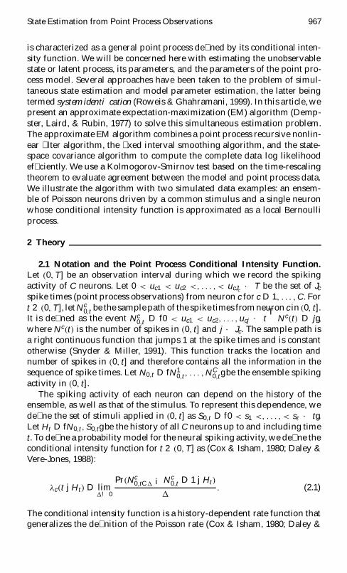
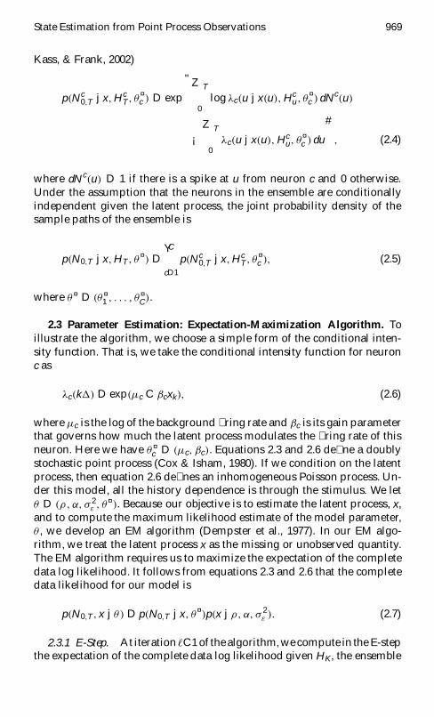
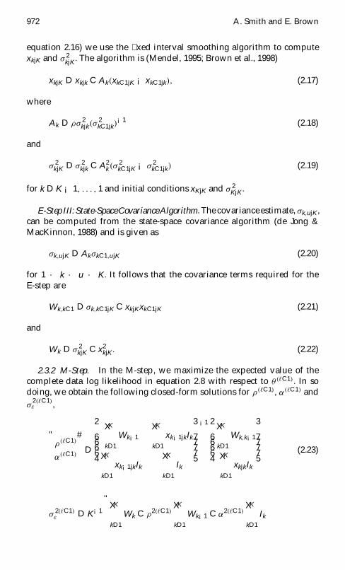
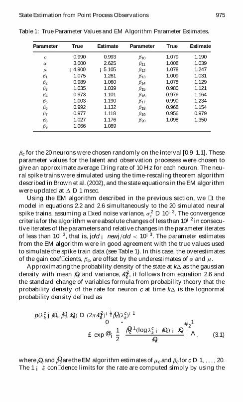
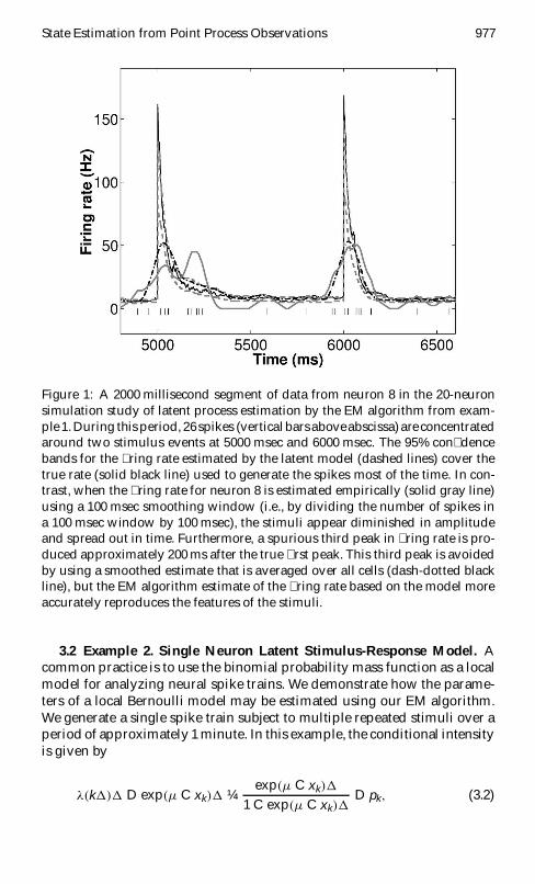
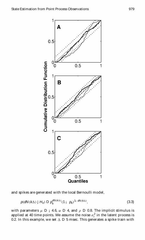
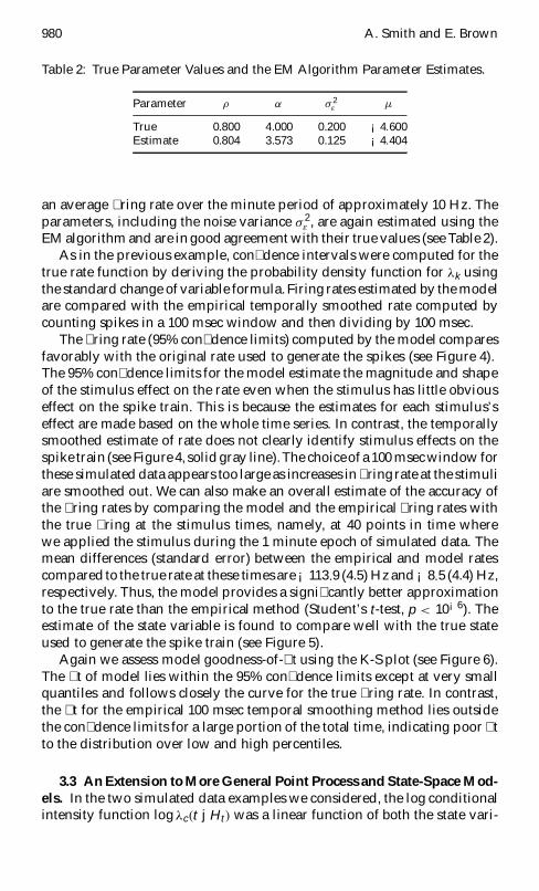
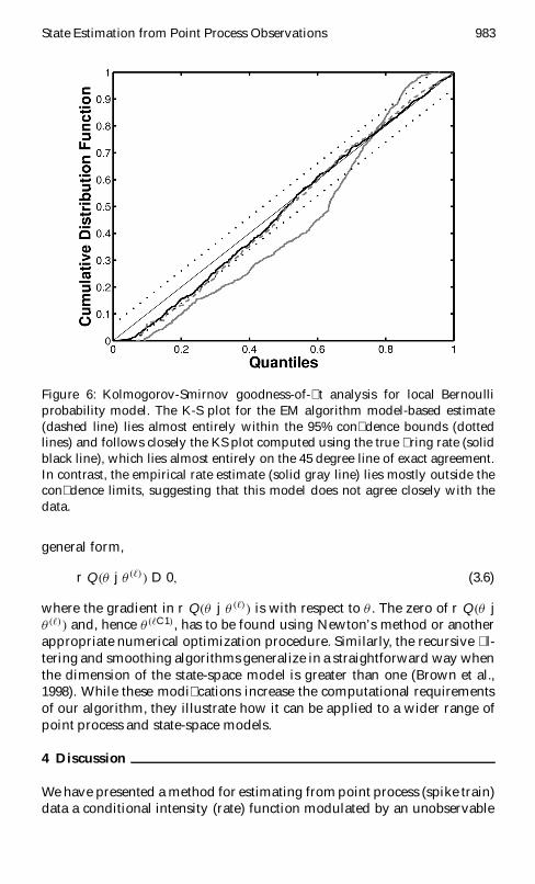