Workflow Analysis and Surgical Phase Recognition in Minimally Invasive Surgery

Oliver Weede, Frank Dittrich, Heinz Wörn Institute for Process Control and Robotics Karlsruhe Institute of Technology (KIT)

Karlsruhe, Germany oliver.weede@kit.edu

Brian Jensen*, Alois Knoll*, Dirk Wilhelm**, Michael Kranzfelder**, Armin Schneider**, Hubertus Feussner**

*Robotics and Embedded Systems **Minimally invasive Interdisciplinary Therapeutical

Intervention (MITI), Technical University München (TUM)

München, Germany

Abstract—In this paper, a new approach is described to recognize the phases of a single-port sigma resection intraoperatively, based on the position signal of the surgical instruments, the endoscopic video and an audio signal, signaling coagulations. Approaches for detecting the coagulation sounds, as well as the instruments visible in the endoscopic video using a bag of words model are detailed. The intervention phases are regarded as classes of a naive Bayes classifier. Features that differentiate intervention phases are examined. The naive Bayes classifier is extended by a dynamic feature, which includes the order of the intervention phases and their duration. First results show that in 93.2% the recognized phases are classified as true positive.

Cognitive medical technology, workflow analysis, high-level task recognition, trajectory segmentation, object recognition, sound recognition

I. INTRODUCTION A key aspect of robot assisted surgery, e.g. single port

surgery, is the relative complexity of the numerous functions that have to be precisely controlled by the surgeon, which effectively mandates an intuitive man-machine interface. A consequence of this requirement is that the system has to be adaptive/cognitive to optimally accommodate the surgeon’s skills. An essential precondition for achieving situation awareness and even cooperative features is modeling the task to be performed – for the purposes of this paper: a laparoscopic sigmoidectomy (sigma resection). Information retrieval, workflow analysis and online action recognition are all crucial components necessary for achieving situational-adaptive behavior of medical devices and robots, carrying out autonomic tasks or aiding context sensitive safety mechanisms and systems which provide context-sensitive information.

In the operating theater of the future all devices in the Operating Room could be integrated together. Information could be gathered and exchanged both for administrative purposes in the hospital, as well as for cooperative interaction and data fusion of all devices in the OR. Further, reasoning and self-documentation based on the aggregated information would be possible. An example for an administrative use case is the optimized scheduling in the hospital based upon an estimation

of the remaining time [4] or automatic self-documentation of the surgical procedure.

The assumption for the recognition of surgical phases is that there is an inherent structure of an intervention of a specific type that is the same for any specific instance of that procedure. Specifically several phases should be identifiable which occur in a specific sequence.

A. Related Works There are works identifying single tasks like suturing [1], in

contrast, in this approach surgical phases of a complete intervention are identified. Neumuth et al. [9] introduced a formal model for a surgical process, a generic framework for providing data, focusing on the conceptual design of a data warehouse and on establishing relevant relationships to model the process. In contrast, we are operating on low-level signals (position signal, audio and endoscopic video signals) and the identification of relevant features to segment an intervention into surgical phases. With the same focus, Ahmadi et al. [2] uses a dynamic time warp algorithm for registering interventions using 17 features, which are common for each of the 14 phases of a cholecystectomy. Intraoperatively a time mapping is performed to obtain the current phase. 92% recognition rate with a tolerance of five seconds was reached. Blum et al. [3] uses Hidden Markov Models to determine phases in the same type of intervention. The authors discussed different HMM topologies to model the process. An overall error of 6.73% could be attained, 18.4% by using just the endoscopic video [4]. Katic et al. [8] are able to recognize four phases in a dental implant surgery based on trajectories with a rule-based, deductive approach (”if-then”-structure) combined with a case-based inductive approach, using an inference mechanism. Features, like “near”, “far”, or “decreasing distance” are defined by fuzzy predicates. A semantic model represents the current situation with description logics. The situation is described by relations between the drilling device and all other objects. Lalys et al. [12] combined a Support Vector Machine and a discrete Hidden Markov Model to segment six phases in a neurosurgical intervention based on a microscope video. SVMs were trained to extract surgical scene

1068

Proceedings of the 2012 IEEEInternational Conference on Robotics and Biomimetics

December 11-14, 2012, Guangzhou, China

information, which is then used as observations for training a discrete HMM. Each phase represents a surgical phase.

Our approach to recognition of surgical phases with a dynamic naive Bayes classification including a feedback loop is new. Furthermore, to our knowledge features like instrument distance, number of coagulations/high frequency coagulations, phase time, normalized movements per minute and number of instrument changes have yet not been considered. Beyond this, the first results in the recognition rate are very promising.

B. Workflow Description of the Sigma Resection The following nine surgical phases are identified for a

single-port sigma resection. The times for the phases are shown in Table I.

1. Dissection / mobilization of descending colon. The right-hand / dominant instrument (DI) is a forceps. The non-dominant instrument is a forceps during the whole intervention.

2. Dissection of colon/sigmoid mesenterium. High frequency coagulations characterize this phase. DI: forceps.

3. Endoscopic transportation of counter-pressure plate into descending colon. DI: forceps

4. Closure of descending colon (proximal stump). In this phase, the first instrument change occurs. DI: linear stapler.

5. Dissection / mobilisation of sigmoid colon. High frequency coagulations and the first use of a scissor are characterizing this phase. DI: forceps and scissor.

6. Specimen retrieval via the rectum. DI: forceps.

7. Closure of the rectal stump using a stapler (distal stump). DI: forceps, stapler, scissor (if needed).

8. Thorn positioning of counter-pressure plate into staple line of descending colon (proximal stump). DI: forceps and scissor.

9. Approximation and coalition of counter-pressure plate with transrectal inserted circular stapler (brace- stitching device), anastomosis. DI: forceps and scissor.

TABLE I. TIME FOR PHASES

Time [Min] Minimum Mean Maximum

Phase 1 3 6.7 30

Phase 2 10 14.0 50

Phase 3 5 6.5 15

Phase 4 3 3.8 15

Phase 5 7 7.3 20

Phase 6 3 3.6 10

Phase 7 4 4.5 20

Phase 8 3 3.9 15

I. DATA AQUISITION Three data sources are fused. The position signal of the

instrument trajectories, an audio signal with sounds, signaling

coagulations and the endoscopic video. The trajectories of two forceps, one scissor and the endoscope are tracked and recorded with the NDI aurora system at a sampling frequency of 40Hz. The audio signal of the high-frequency surgical unit is synchronized to the trajectory, as well as the video from the endoscopic camera. The stapler is not tracked, but recognized in the endoscopic video. Three interventions in an animal experiment were recorded. Eight artificial trajectories were added, created by cutting out parts of the trajectory, which do not necessary belong to the intervention (e.g. explanations about the anatomy, inspection of the surgical site, times for preparing external instruments). In addition, the time used for instrument changes was varied, few coagulations were inserted or left out and few millimeters position offset was introduced to parts of the intervention. The trajectories were annotated with nine phases determined by the clinical partners. However, phase nine is excluded because of problems during the intervention and the recording process.

A. Detection of Coagulation Sounds in an Audio Signal The audio signal of the high-frequency surgical unit is

signaling coagulations by a static, harmonic sound. The aim is to detect these sounds and the corresponding locations of the dominant surgical instrument.

Learning Structure of Coagulation Sound. A short term spectral analysis of the audio signal x(n) with a sampling frequency of fS=22.05 kHz is performed. Therefore, a FFT with length 4096, 50% overlap and a blackman window is resulting in an N-point DFT magnitude spectrum |X[k]|=|FFT[x(n),N]|/N, N=1024. We determine four dominant frequency peaks at the frequencies 220.7Hz, 441.4Hz, 1313.5Hz and 2185.6Hz (coefficients k=40, 81, 243, 405) and their amplitude ratio. The DFT serves as a band pass filter with 1024 bands. To detect the sound we consider the four frequency bands represented by these coefficients.

Detecting the Coagulation Sound. An envelope follower is summing the amplitude of all DFT-coefficients over a time of two seconds for determining a noise threshold tn. If the amplitude in a band is greater than the threshold tn a gate opens and the energy in the band is summed up. For each band a detection threshold td is determined depending on the learned amplitude of the regarded band and the noise threshold tn. If the summed energy is greater than td, this indicates a detection of the coagulation sound. Fig. 1 shows both thresholds, the

Figure 1. Amplitude of coefficent (blue), Noise threhold (green), Detection threhold (black), summed energy (red) indicating a coagulation sound.

1069

summed energy and the signal itself for the first band.

The pattern is classified as a coagulation sound, if the duration and the energy are in between a specified interval for each of the four bands. The detection algorithm was evaluated in two interventions with 27 and 62 coagulations. There was no false classification and 96.3% of the coagulations were recognized.

B. Image Processing - Detecting Instruments In order to augment the tracking and audio information

visual classification labels were extracted from the recorded endoscopic video data. This was accomplished using a general bag of words video classification strategy as described by Zhang et al. [10]. The aim of the visual classification algorithm is to label each input video frame according to whether, and if so, which of the surgical instruments are visible (forceps, stapler, scissors).

The Bag of Words Model for Visual Classification. In general the bag of words model for visual classification as implemented in this paper can be broken down into the following steps:

1. Extract a sparse set of image feature descriptors from all training images.

2. Perform clustering on the extracted feature descriptors using clustering algorithm. The resulting cluster centers represent the visual words.

3. Associate each feature descriptor with the appropriate corresponding visual word. Generate a histogram of the occurrences of each visual word for each training image.

4. Feed the training set consisting of labels and corresponding visual word histograms into a discriminative classifier.

After training image classification is accomplished by extracting feature descriptors, then generating a visual word histogram, which is used as input into the discriminative classifier.

Training Parameters. As the initial step in our implementation a spare set of SIFT [11] features are detected and the descriptors are extracted from each training image. Clustering over all feature descriptors in the training set is performed using k-Means. A cluster count Wc of 1000 clusters was chosen. Fig. 2 shows the extracted SIFT features in an image containing the stapler.

A linear Support Vector Machine (SVM) was used for classification with the additional constraint of a L1 regularization parameter to enforce sparsity of the support vectors. To compensate the unbalanced number of training samples in each label class, the classes were weighted inverse proportionally to their frequency in the training set, thus reducing the classification bias inherent towards the classes with the most training data. To include color information into the training set and thus further improve recognition accuracy each visual word histogram was extended with a color

histogram from the corresponding training image reduced to 32 bins per color channel to reduce the size of the training vectors.

Figure 2. Example of the extracted feature descriptors from image contaning the stapler.

Classification Accuracy. A total of 3210 training images were extracted from the endoscope video recordings. The training images for each class were divided up by an 80/20 split, with 80% of the images used in training and 20% selected at random and used exclusively for testing. The amount of training images for each class is listed in Table II.

TABLE II. TRAINING IMAGE SET DISTRIBUTION

Class Empty Forceps Scissors Stapler

Size 1653 1216 68 273

The experimental results achieved after training for each of

the label classes using the testing data set is listed in Table III.

TABLE III. CLASSIFICATION RESULTS FOR EACH OF THE LABELS

Class Precision Recall F-Score Empty 93.0% 90.3% 91.8% Forceps 86.1% 89.6% 87.9% Scissors 75.0% 58.0% 65.4% Stapler 87.6% 92.2% 89.9%

II. FEATURES FOR SURGICAL PHASE CLASSIFICATION Twelve features are extracted from the trajectory defining a

multi dimensional feature vector x for each point in time. Each feature is discrete.

A. Instrument Changes and Instument Identification To determine whether any of the end-effectors are inside the

patient, a frontal plane is defined in the height of the navel. The trajectories are traversed. If the trajectory of an end-effector dissects the plane from upside to downside and the distance to the port is less than a threshold tport=5 cm, the point of the trajectory is labeled as “inside”. If the trajectory is inside and an end-effector dissects from downside to upside near to the port, an instrument change is detected. Instrument changes with less than 5 seconds gap from the previous change are suppressed.

Feature x1: The number of instrument changes of the

1070

tracked instruments that have occurred since the beginning of the intervention. Parts of the trajectory with less than two instruments labeled as “inside” are omitted (for all following features). The non-dominant instrument is always inside the patient.

Feature x2: The instrument in use. Identification 1 denotes the use of a forceps for the dominant instrument, Identification 2 denotes the stapler and identification 3 denotes a scissor.

B. Path length, Velocity and Distance beetween Instruments Feature x3: The current path length of the dominant

instrument is computed and quantized to decimeters.

Feature x4 and x5: The instant velocity of the dominant and the non-dominant end-effectors are computed regarding a three second window. The velocities are quantized to five clusters with centers 18 (burst), 12 (fast), 7 (mid tempo), 3 (slow) and 0.75 (no movement) cm/sec. The quantization steps where always obtained by a k-Means clustering of the regarded feature in the training set.

Feature x6: The distance between the left and the right end-effector is measured, clustered and quantized to the cluster center 3 (working closely together), 6, 9 and 17cm (far distance).

C. Number of Coagulations, High Frequency Coagulations, Number of High Frequency Coagulations

Feature x7: At each point in time the number of coagulations since the beginning of the intervention is computed.

Feature x8: To determine high frequency coagulations, the number of coagulations in a time window of 60 seconds is computed. The values are quantized to the values 0, 2, 4 and 6. Values greater than two are so called “high frequency coagulations”.

Feature x9: Because the number of coagulations varies strongly in several interventions but there are typically agglomerations connected to intervention phases, the feature “number of high frequency coagulations” is introduced: If the quantized signal is greater than two and releases to zero a “high frequency coagulation counter” is increased. This feature is also added to the feature vector.

D. Coagulation Regions Feature x10: The regions, where coagulations are necessary

are especially important for the intervention. To determine these areas, the positions of the trajectories where coagulations occur are clustered with the k-Means algorithm. Each point of the trajectory is classified to one of these clusters with a Bayes classifier (c.f. [5]). We use only a very rough division of the workspace into five regions due to the anatomical diversity. The classification includes a threshold of 3cm. If the distance of a point of a trajectory is greater than 3cm from any cluster center, the point of the trajectory is classified to a dummy class.

E. Activity – Normalized Movements Per Minute Feature x11: The concept movements per minute is

introduced by Datta et al. in the context of surgical skill assessment [6]. The number of maxima in the low-pass filtered velocity curve is an indicator for the expertise of a surgeon. Some steps in an intervention need more movements per minute than others. To eliminate any differences in expertise, we normalize the movements per minutes signal by dividing it with the average number of movements since the beginning of the intervention. This feature, determined for the dominant instrument, measures a degree of activity.

F. Instruments in Field of View Feature x12 describes by an identification number, which

instrument are visible in the endoscopic video: 1: empty, 2: stapler, 3: scissor, 4: forceps, 5: scissor and forceps, 6: forceps and stapler, 7: scissor and stapler.

G. Time for Next Phase The phase itself should be included as a feature, because

there is a specific order, in which the phases are performed. Time is a crucial point, if there are complications in an earlier phase, absolute time (time since the beginning of the intervention) will be a false indicator for determining the current phase. Thus, instead of using absolute time, the time since the beginning of the surgical phase is introduced and combined with the order of phases: At each timestamp it in phase i, the probability of a change into a next phase k is determined. This feature extends the naive Bayes classifier with dynamics. The concept is discussed detailed in Section III. B.

III. DYNAMIC NAIVE BAYES CLASSIFICATION At each point in time, in the training phase, as well as

intraoperatively, the mentioned features are combined to a feature vector x and are classified.

A. Bayes Classification The intervention phases are modeled as 8K classes

KiCi ,...,1, . The posterior probability of class iC can be computed as

K

kkk

iii

CPCP

CPCPCP

1

)|()(

)|()()|(x

xx

In respect to the frequentist view, the prior probability KiCP i ,...,1),( is computed as the relative frequency of

occurrence of phase i with respect to all trajectories of the supervised learning phase. The probability distribution

)|( iCP x contains the d dimensional feature vector x . We use the mentioned d=12 features.

The assumption of the naive Bayes classifier is, that the components are independent and therefore the probability distribution )|( iCP x can be computed by

1071

d

jiji CxPCP

1

)|()|(x . (1)

Phase iC is selected, if ).|(max)|( xx kki CPCP

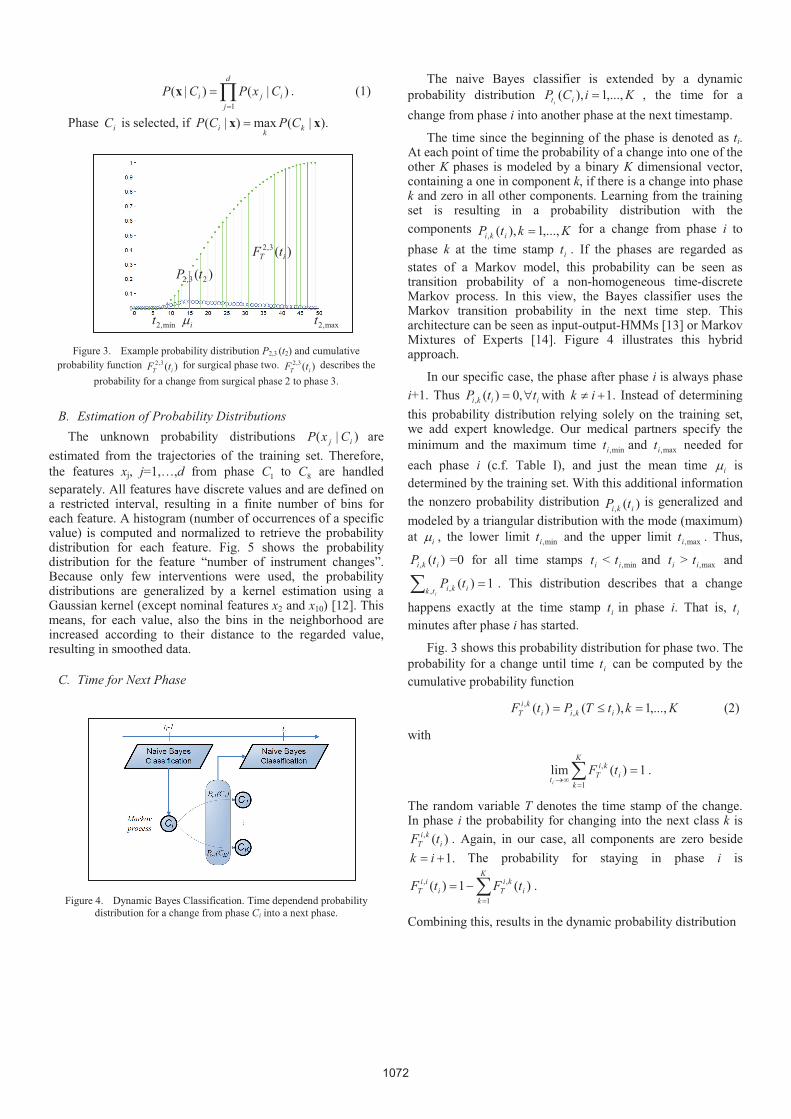
Figure 3. Example probability distribution P2,3 (t2) and cumulative probability function )(3,2

iT tF for surgical phase two. )(3,2iT tF describes the

probability for a change from surgical phase 2 to phase 3.

B. Estimation of Probability Distributions The unknown probability distributions )|( ij CxP are

estimated from the trajectories of the training set. Therefore, the features xj, j=1,…,d from phase 1C to 8C are handled separately. All features have discrete values and are defined on a restricted interval, resulting in a finite number of bins for each feature. A histogram (number of occurrences of a specific value) is computed and normalized to retrieve the probability distribution for each feature. Fig. 5 shows the probability distribution for the feature “number of instrument changes”. Because only few interventions were used, the probability distributions are generalized by a kernel estimation using a Gaussian kernel (except nominal features x2 and x10) [12]. This means, for each value, also the bins in the neighborhood are increased according to their distance to the regarded value, resulting in smoothed data.

C. Time for Next Phase

Figure 4. Dynamic Bayes Classification. Time dependend probability distribution for a change from phase Ci into a next phase.

The naive Bayes classifier is extended by a dynamic probability distribution KiCP iti

,...,1),( , the time for a change from phase i into another phase at the next timestamp.

The time since the beginning of the phase is denoted as ti. At each point of time the probability of a change into one of the other K phases is modeled by a binary K dimensional vector, containing a one in component k, if there is a change into phase k and zero in all other components. Learning from the training set is resulting in a probability distribution with the components KktP iki ,...,1),(,

for a change from phase i to phase k at the time stamp it . If the phases are regarded as states of a Markov model, this probability can be seen as transition probability of a non-homogeneous time-discrete Markov process. In this view, the Bayes classifier uses the Markov transition probability in the next time step. This architecture can be seen as input-output-HMMs [13] or Markov Mixtures of Experts [14]. Figure 4 illustrates this hybrid approach.

In our specific case, the phase after phase i is always phase i+1. Thus iiki ttP ,0)(, with .1ik Instead of determining this probability distribution relying solely on the training set, we add expert knowledge. Our medical partners specify the minimum and the maximum time min,it and max,it needed for each phase i (c.f. Table I), and just the mean time i is determined by the training set. With this additional information the nonzero probability distribution )(, iki tP is generalized and modeled by a triangular distribution with the mode (maximum) at i , the lower limit min,it and the upper limit max,it . Thus,

)(, iki tP =0 for all time stamps it < min,it and it > max,it and

1)(, ,

itk iki tP . This distribution describes that a change

happens exactly at the time stamp it in phase i. That is, it minutes after phase i has started.

Fig. 3 shows this probability distribution for phase two. The probability for a change until time it can be computed by the cumulative probability function

KktTPtF ikiiki

T ,...,1),()( ,, (2)

with

1)(lim1

,K

ki

kiTt

tFi

.

The random variable T denotes the time stamp of the change. In phase i the probability for changing into the next class k is

)(,i

kiT tF . Again, in our case, all components are zero beside

.1ik The probability for staying in phase i is K

ki

kiTi

iiT tFtF

1

,, )(1)( .

Combining this, results in the dynamic probability distribution

)(3,2iT tF

)( 23,2 tP min,2t i max,2t

1072

)( it CPi

(3)

T

iKi

Tiii

T

K

ki

kiTi

iiTi

iT tFtFtFtFtF )(),...,(,)(1),(),...,( ,1,

1

,1,1, .

If in phase i the only probability is to change into phase i+1, then component i is monotonically decreasing from one to zero, reached at time max,it , and component i+1 is monotonically increasing from zero to one, reached at the same time. All other components stay zero. Thus, a change into the next phase is impossible before min,it is reached, becomes more and more probable and after max,it minutes necessary.

Summarizing, phase pC is selected with

d

jijiti

iCxPCPCPp

i1

)|()()(maxarg (4)

Figure 5. Example probability distribution )|( 1 iCxP of the number of instrument changes x1 in the intervention. Phases 1 to 8. Zero changes in

phases 1 to 3.

IV. RESULTS The evaluation was performed with six interventions, one

unvaried intervention and five artificial generated trajectories. None of the interventions used for the evaluation was included in the training set. At each point of time, the classified phase was compared to the phase annotated by the expert. A false classification is regarded as failure. 6.8 % of the classifications where failures with a standard deviation of 3.8 (true negative rate), 93.2% of the time stamps are true positive. Table IV shows the failure rate just using single features.

Path length is the most significant feature. Absolute time was only added as a reference. The combination of these independent features shows better results than any of the single features taken in isolation. Even the features, which distinguish least, like velocity of the non-dominant instrument or instrument distance, add a benefit to the classification. For example, the action of grasping and pulling soft tissues away could be described by a large distance between the instruments, with no movement in the left-hand instrument and slow movement in the dominant instrument. This occurs rarely in

phases 3, 5 and 6, but very often in 4. The action of actively working together with both instruments while coagulations occur could be described as a low distance between the instruments, while both instruments are moving slowly, combined with a nonzero coagulation frequency. This combination just occurs in phases 2 und 5. No instrument changes since the beginning of the intervention implies the current phase could be 1, 2 or 3. The use of forces implies that the phase is not 1, 2, 3, 4 or 6. There are more movements per minute in phases 2, 4 and 5 than in the other phases. High frequency coagulations only occur in phase 1, 3 and 4.

TABLE IV. ABSOLUTE FAILURE OF SEPERAT FEATURES

Mean [%] Standard deviation

x3: Path (dominant instrument) 23.7 5.6

Time (absolut) 38.9 21.7

x7: Number of coagulations 47.5 13.0 x9: Number of high frequency coagulations 50.4 14.2

x12: Instruments in field of view 65.5 7.5 x1: Number of instrument changes 65.8 7.4

x2: Instrument used 66.0 5.8

x11: Activity 76.1 8.3

x4: Velocity (dominant instrument) 83.7 3.7

x8: Coagulation frequency 84.9 3.5

x10: Coagulation regions 85.3 3.1

x6: Instrument distance 85.9 3.1

x5: Velocity (non-dominant instrument) 91.3 1.9

V. CONCLUSION, DISCUSSION AND FUTURE WORK The Bayes approach has the advantage, e.g. compared with

neural networks, of human orientated data representation. The probability distributions of the features in each class are easy to interpret and can also be used to model expert knowledge manually, e.g. by a proposition like “In phase closure of the rectal stump one to five instrument changes have occurred, the mean is three.” The quantized values for the features are also plain, e.g. low, mid and high distance between the tips.

Segmenting an intervention into phases can also be used for improved automatic surgical skill assessment by evaluating the features which distinguish levels of expertise, like path length or movements per minutes, separately for different phases [7]. We are planning on developing a robot assisted autonomous camera guidance system for minimally invasive surgery that will be based upon the surgical phase recognition methods discussed in this paper, learning optimal camera positions appropriate for the current estimated surgical phase.

The recognition rate of 96.3% of the coagulation sounds seems to be sufficient and can easily be improved by acoustic shielding. Also, the F-score of 89.9% in recognizing the stapler seems to be sufficient, because the stapler is generally visible for periods of at least one minute at time when in use, thus its

1,2,3 4 5 6 7 8

1073

presence can be detected with almost certainty. In general the instrument recognition results achieved in this paper demonstrate the effectiveness of employing a bag of words model involving spare SIFT features together with a linear SVM for object recognition purposes in a clinical setting. The approach is real-time capable. The detection of the instruments can be performed in 500 to 700 ms (single threaded, Intel Core i7) where the feature point extraction is most time-consuming. The other steps of the phase recognition are negligible. We believe that our approach for recognizing the surgical phases can be generalized to other interventions and would also serve very promising results. By including the class itself and a time dependent order of the classes, we added a feedback and dynamics to the naive Bayes classifier. Especially this concept for including any order of surgical phases makes this approach generic.

ACKNOWLEDGMENT The present research was conducted within the setting of the

research group “Single Port Technology” FOR 1321 founded by the German Research Foundation.

REFERENCES

[1] S. Speidel, T. Zentek, G. Sudra, T. Gehrig, B. Müller, C.Gutt, R. Dillmann, “Recognition of Surgical Skills using Hidden Markov Models,” Progress in biomedical optics and imaging, vol. 10 (2), no37, 2009.

[2] S.A. Ahmadi, T. Sielhorst, R. Stauder, M. Horn, H. Feussner und N. Navab, “Recovery of Surgical Workflow Whithout Explicit Models”, MICCAI 2006, pp. 420-428

[3] T. Blum, N. Padoy, H. Feussner and N. Navab, “Modeling and Online Recognition of Surgical Phases Using Hidden Markov Models”, MICCAI 2008, pp. 627-635

[4] T. Blum, H. Feußner, N. Navab, „Modeling and Segmentation of Surgical Workflow from Laparascopic Video“, MICCAI 2010.

[5] O. Weede, D. Stein, N. Gorges, B. Müller and H. Wörn., “A Cognitive Path-Guidance-System for Minimally Invasive Surgery”, In IEEE Int. Symp. on Intelligent Systems and Informatics, 2010, pp. 139 – 144.

[6] V. Datta, S. Mackay, A. Darzi and D. Gillies, “Motion analysis in the assessment of surgical skill”. Comput Methods Biomech Biomed Eng., 2001, pp. 515-523.

[7] M.T. Boll, O. Weede, U. Kühnapfel, G. Bretthauer, H. Wörn, „Automatisierte Bestimmung von Merkmalen zur Bewertung minimal invasiver Eingriffe an einem Pelvitrainer basierend auf Positionsdaten und einer Segmentierung“, Automatisierungstechnische Verfahren für die Medizin, 9. Workshop, Tagungsband. Fortschr.-Ber. VDI Reihe 17 Nr. 279, 2010, pp. 61-62.

[8] D. Katic, G. Sudra, S. Speidel, G. Castrillon-Oberndorfer, G. Eggers and R. Dillmann, “Knowledge-based Situation Interpretation for Context-aware Augmented Reality in Dental Implant Surgery” Proc. Medical Imaging and Augmented Reality, 2010, pp. 531-540.

[9] T. Neumuth, S. Mansmann, M.H. Scholl and O. Burgert, “Data Warehousing Technology for Surgical Workflow Analysis”, IEEE Int. Symposium on Computer-Based Medical Systems, 2008, pp. 230-235.

[10] J. Zhang, M. Marszalek, S. Lazebnik, and C. Schmid. Local features and kernels for classification of texture and object categories: A comprehensive study. IJCV, 73(2):213–238,June 2007

[11] D. Lowe. Distinctive image features form scale-invariant keypoints. International Journal of Computer Vision, 60(2):91–110, 2004.

[12] E. Parzen. On estimation of a probability density function and mode. Annals of Mathematical Statistics 33: 1065–1076, 1962.

[13] Y. Bengio and P. Frasconi. Input-Output HMMs for Sequence Processing. IEEE Transactions on Neural Networks 7: 1231-1249, 1996.

[14] M. Meila and M.I. Jordan. Learning Fine Motion by Markov Mixtures of Experts. Advance in Neural Information Processing Systems 8, pp. 1003-1009, 1996.

1074