
Workbook on Numerical Modeling - UAF home · iii This workbook is complementary to the course based...
214
Zygmunt Kowalik Institute of Marine Science University of Alaska, Fairbanks Workbook on Numerical Modeling Fairbanks, 2003
Transcript of Workbook on Numerical Modeling - UAF home · iii This workbook is complementary to the course based...
Zygmunt KowalikInstitute of Marine Science
University of Alaska, Fairbanks
Workbook
on
Numerical Modeling
Fairbanks, 2003
i
Table of Contents
Chapter I: Problems in Transport Equations . . . . . . . . . . . . 11. Vertical coordinate . . . . . . . . . . . . . . . . . . . . . . 1Problem No.1, explicit time marching withdirectional derivative in space . . . . . . . . . . . . . . . . . . 3Problem No.2, explicit time marching andcentral derivative in space . . . . . . . . . . . . . . . . . . . . 7Problem No.3, simple correction scheme . . . . . . . . . . . . . . 9Problem No.4, QUICKEST method . . . . . . . . . . . . . . . . 11Problem No.5, stability parameter . . . . . . . . . . . . . . . . 14Upwind scheme . . . . . . . . . . . . . . . . . . . . . . . . . 14Central space derivative and forward time derivative . . . . . . . . . 17Central space derivative and central time derivative . . . . . . . . . 172. Flux form of convective/advective transport . . . . . . . . . . . 21Problem No.6, computation of the convective transportby the first order scheme using fluxesand upstream/downstream spatial discretization . . . . . . . . . . 22Problem No.7, computation of the convective transportby the second order scheme using fluxesand upstream/downstream spatial discretization . . . . . . . . . . 26Problem No.8, computation of the convection by the third oderscheme using fluxes and upstream/downstream spatial discretization . 31Problem No.9, computation of the advection by the thirdorder scheme using fluxes and upstream/downstreamspatial discretization (geometry along x direction) . . . . . . . . . . 37Problem No.10, computation of the convectionby Flux–Corrected–Method (FCT) . . . . . . . . . . . . . . . . 38
Chapter II: Two-Dimensional Models . . . . . . . . . . . . . . . . 451. Propagation in channel . . . . . . . . . . . . . . . . . . . . 45Problem No. 1, solution by Fisher method . . . . . . . . . . . . . 46Problem No. 2, solution by leap-frog method . . . . . . . . . . . . 48Problem No. 3, solution by corrected leap-frog method . . . . . . . 53Problem No. 4, numerical stability . . . . . . . . . . . . . . . . 592. Run-up in channel . . . . . . . . . . . . . . . . . . . . . . 64Problem No. 5, calculation of the run-up in channel . . . . . . . . . 65Problem No. 6, propagation in sloping channel – nonlinear terms . . . 693. Rectangular and non-rectangular water bodies . . . . . . . . . . 78Problem No. 7, storm surge in the rectangular domain . . . . . . . 81
ii
Problem No. 8, storm surge in the non-rectangular domain . . . . . 90Problem No.9, storm surge in the rectangular domain -migration to Fortran 90 . . . . . . . . . . . . . . . . . . . . . 98Problem No.10, storm surge in the non-rectangular domain -migration to Fortran 90 . . . . . . . . . . . . . . . . . . . . 102
Chapter III: Three-Dimensional Models . . . . . . . . . . . . . 109Problem No. 1, vertical direction . . . . . . . . . . . . . . . . 109Problem No. 2, 3D - barotropic model . . . . . . . . . . . . . 116Problem No. 3, 3D - barotropic model, sigma coordinate . . . . . 131Introduction . . . . . . . . . . . . . . . . . . . . . . . . . 131How to write code in the nonrectangular domain . . . . . . . . . 132Problem No. 4, 3D - baroclinic model, sigma coordinate . . . . . . 168
Appendix: Basic Mathematical Formulas . . . . . . . . . . . . 205Rudiments of trigonometry . . . . . . . . . . . . . . . . . . . 205Rudiments of complex number theory . . . . . . . . . . . . . . 207Rudiments of algebra . . . . . . . . . . . . . . . . . . . . . 209Rudiments of power series and integration . . . . . . . . . . . . 210
iii
This workbook is complementary to the course based on thebook by Z. Kowalik and T.S. Murty entitled: Numerical Modelingof Ocean Dynamics, Published by: World Scientific Publishing Co.,Singapore, New Jersey, London, 1993.
The purpose of this workbook is to apply fundamentals ofcomputer simulation described in Numerical Modeling of OceanDynamics (NM) to the short practical projects for the real hands–on experience in applying numerical methods. We assume thatthe reader possesses experience with FORTRAN. The workbookwill follow the material described in NM and solve simple problemsthrough FORTRAN programs. It contains short descriptions of theprograms. All programs are copied onto diskette, which is also in-cluded. We will confine ourselves to transport equations (diffusionand advection), shallow water phenomena – tides, storm surges andtsunamis, and three-dimensional time dependent oceanic motion.
PROBLEMS IN TRANSPORT EQUATIONS 1
CHAPTER I
PROBLEMS IN TRANSPORT EQUATIONS
1. Vertical coordinate
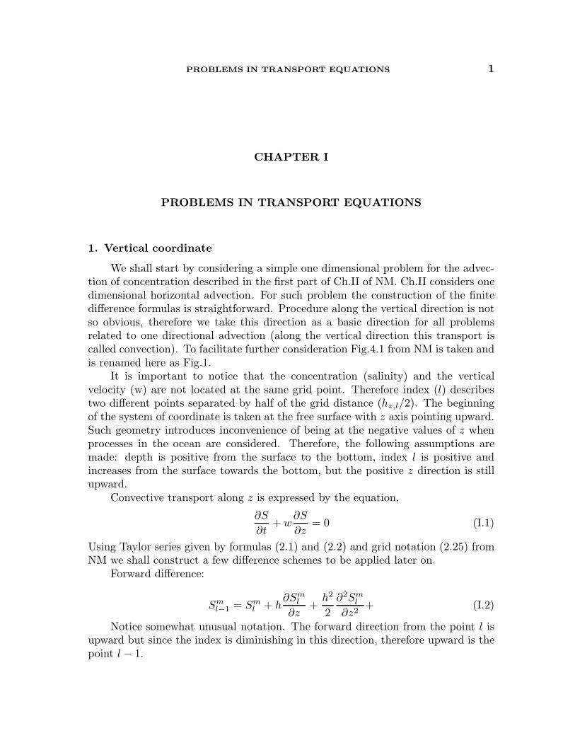
We shall start by considering a simple one dimensional problem for the advec-tion of concentration described in the first part of Ch.II of NM. Ch.II considers onedimensional horizontal advection. For such problem the construction of the finitedifference formulas is straightforward. Procedure along the vertical direction is notso obvious, therefore we take this direction as a basic direction for all problemsrelated to one directional advection (along the vertical direction this transport iscalled convection). To facilitate further consideration Fig.4.1 from NM is taken andis renamed here as Fig.1.
It is important to notice that the concentration (salinity) and the verticalvelocity (w) are not located at the same grid point. Therefore index (l) describestwo different points separated by half of the grid distance (hz,l/2). The beginningof the system of coordinate is taken at the free surface with z axis pointing upward.Such geometry introduces inconvenience of being at the negative values of z whenprocesses in the ocean are considered. Therefore, the following assumptions aremade: depth is positive from the surface to the bottom, index l is positive andincreases from the surface towards the bottom, but the positive z direction is stillupward.
Convective transport along z is expressed by the equation,
∂S
∂t+ w
∂S
∂z= 0 (I.1)
Using Taylor series given by formulas (2.1) and (2.2) and grid notation (2.25) fromNM we shall construct a few difference schemes to be applied later on.
Forward difference:
Sml−1 = Sm
l + h∂Sm
l
∂z+
h2
2∂2Sm
l
∂z2+ (I.2)
Notice somewhat unusual notation. The forward direction from the point l isupward but since the index is diminishing in this direction, therefore upward is thepoint l − 1.

2 PROBLEMS IN TRANSPORT EQUATIONS
j − 1 j j + 1
l + 1
l
l − 1
free surfacez
x
Dz
Dh NhNz
u
w
hz,l−1
hz,l
hz,l+1
bottom
salinity
.............................................................................................................................................................................................................................................................................................................................................................................
........
........
........
........
........
........
........
........
..............................................................................................................................................................................................................................................................................................
•
•
........
........
........
........
........
.................
................
...................................................... ................
........................
........................
..................................
..................................................................................... ........
........
........
........
..................
................
................................................................................................................
............. ............. ............. ............. ............. ............. ............. ............. .............
............. ............. ............. ............. ............. ............. ............. ............. ............. ............. ............. .............
............. ............. ............. ............. ............. ............. ............. ............. ............. ............. ............. .............
............. ............. ............. ............. ............. ............. ............. ............. ............. ............. ............. .............
............. ............. ............. ............. ............. ............. ............. ............. ............. ............. ............. .............
.............
.
.
.
.
.
.
............. . . . . .
Fig. 1Numerical grid distribution in the x–z plane.
Dotted rectangle contains variables with the same j, l indices.
Backward difference:
Sml+1 = Sm
l − h∂Sm
l
∂z+
h2
2∂2Sm
l
∂z2+ (I.3)
Similar formulas can be written for the time derivative, but here both indexand time increase in the same direction, thus;
Sm+1l = Sm
l + T∂Sm
l
∂t+
T 2
2∂2Sm
l
∂t2+ (I.4)
EXPLICIT TIME–DIRECTIONAL DERIVATIVES IN SPACE 3
Sm−1l = Sm
l − T∂Sm
l
∂t+
T 2
2∂2Sm
l
∂t2+ (I.5)
Problem No. 1, explicit time marching with directionalderivatives in space
We start by considering an upwind-downwind formulation for the space deriva-tive and first order approximation for the time marching. We are looking for theformulas similar to (2.54) given in NM. With the help of formula (I.4) the timederivative can be expressed as
∂S
∂t� Sm+1
l − Sml
T(I.6)
Space derivative will be constructed according to the direction of velocity atthe grid point l. If velocity is positive (upward) then
∂S
∂z� Sm
l − Sml+1
h, (I.7)
and, if current direction is negative (downward) then
∂S
∂z� Sm
l−1 − Sml
h(I.8)
Velocity in the concentration grid point l can be expressed as an average wa =0.5(wl + wl+1). Velocities along the positive and negative directions in the gridpoint l are defined as;
wp = 0.5(wa + abs(wa)) wn = 0.5(wa− abs(wa)) (I.9)
Using above formulas the following numerical analog of (I.1) can be constructed;
Sm+1l − Sm
l
T+ wp
Sml − Sm
l+1
h+ wn
Sml−1 − Sm
l
h= 0 (I.10)
Introducing notation used below in the program fluxdir.f,
h = H = HS, TOH = T/HS
FLP = WP (SO(L) − SO(L + 1)), FLN = WN(SO(L− 1) − SO(L))
one can write formula to update salinity value,
SN(L) = SO(L) − TOH(FLP + FLN) (I.11)
4 EXPLICIT TIME–DIRECTIONAL DERIVATIVES IN SPACE
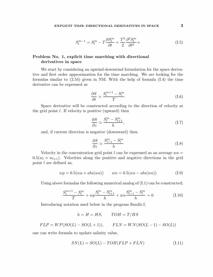
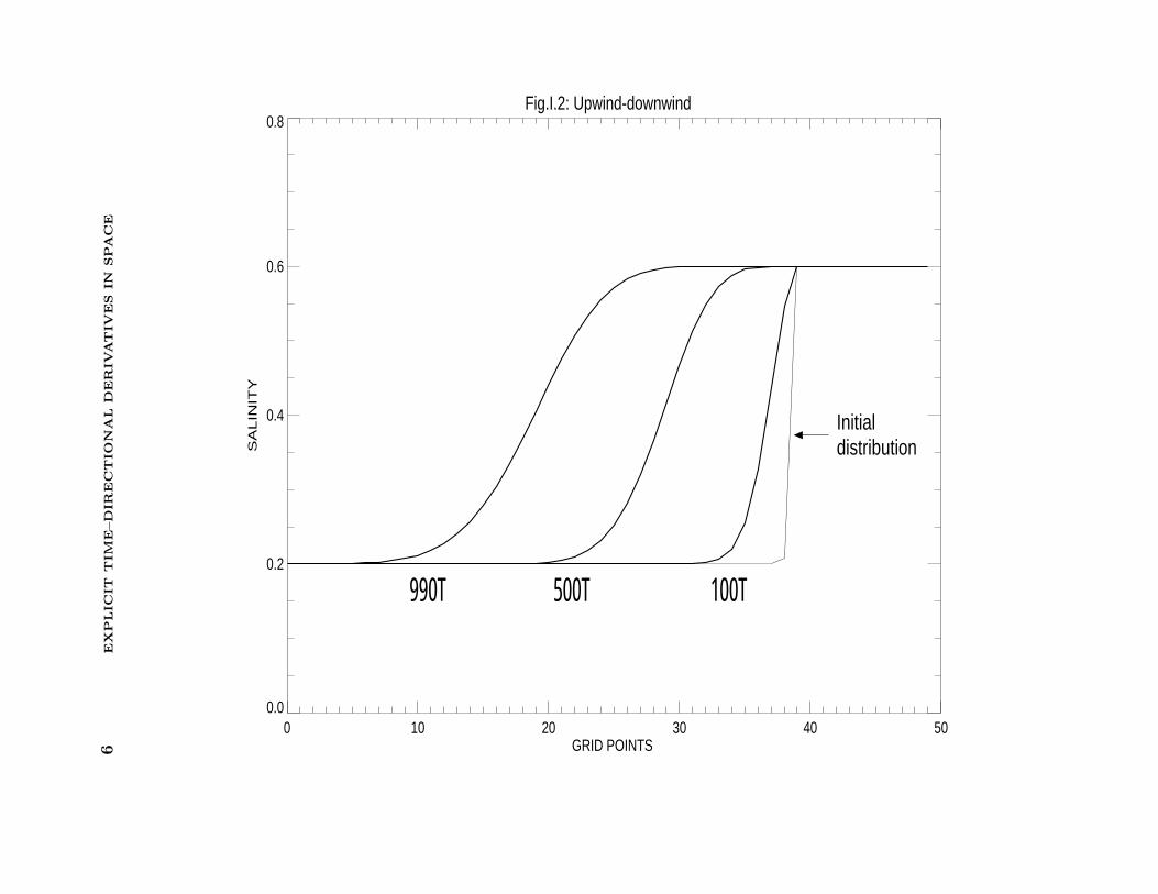
Even though the FORTRAN program is written to account for the variable velocityin space (wl) and the variable space step h = hz(l), in this computation the spacestep is taken as constant h = hz(l) = hs = 5cm and the vertical velocity is also setconstant wl = 10−4cm/s. The time step is T = 1000s. The domain is 2.5m longin the vertical direction, therefore there are 50 grid points in this domain. Initialsalinity distribution is 0.2 from 1 to 39 grid point and 0.6 from 40 to 50 grid point.The old value of salinity Sm
l is called in the program SO and the new value Sm+1l
is named SN.The results of computation are depicted in Fig.2. The initial jump of salinity
propagates downstream and slowly changes its shape due to numerical diffusion.(see explanation in NM given on page 52).
======================================================C PROGRAM TO CALCULATE CONVECTION BY upwind DERIVATIVESC CALCULATIONS ARE MADE IN CGS UNITSC PROGRAM FLUXDIR.FPARAMETER (LZZ=50)REAL W(LZZ),SO(LZZ),SN(LZZ),HZ(LZZ)T=1000. ! TIME STEPMON=1000 !TOTAL NUMBER OF TIME STEPSDO L=1,LZZ-1HZ(L)=5. ! SPACE STEPEND DOC BECAUSE HZ(L)=HS=CONSTHS=5.C INITIAL DISTRIBUTIONDO L=1,39SO(L)=0.2END DODO L=40,LZZSO(L)=0.6END DOOPEN(UNIT=3,NAME=’SOZ1.VER’,STATUS=’UNKNOWN’)C SET VERTICAL VELOCITYDO L=1,LZZW(L)=1.0E-4END DOC START TIME LOOP50 N=N+1C WRITE SALINITY AT TIME STEP 2, 100, 500, 990.IF(N.EQ.2.OR.N.EQ.100.OR.N.EQ.500.OR.N.EQ.990)THENWRITE(3,*)(SO(L),L=1,LZZ)
EXPLICIT TIME–DIRECTIONAL DERIVATIVES IN SPACE 5
END IFTOH=T/HSC CALCULATE NEW VALUE OF SALINITY SNDO L=2,LZZ-1wa=0.5*(w(l)+w(l+1))wp=0.5*(wa+abs(wa))wn=0.5*(wa-abs(wa))FLP=WP*(SO(L)-SO(L+1))FLN=WN*(SO(L-1)-SO(L))SN(L)=SO(L)-(FLP+FLN)*TOHEND DOC KEEP BOUNDARY CONDITIONSSN(LZZ)=0.6SN(1)=0.2C CHANGE VARIABLESDO L=1,LZZSO(L)=SN(L)END DOC STOP COMPUTATION AT TIME STEP MONIF(N.EQ.MON) GO TO 18C RETURN BACK TO 50 TO REPEAT TIME LOOPGO TO 5018 CONTINUEEND
6EX
PLIC
ITT
IME–D
IREC
TIO
NA
LD
ER
IVAT
IVES
INSPA
CE
Fig.I.2: Upwind-downwind
0 10 20 30 40 50GRID POINTS
0.0
0.2
0.4
0.6
0.8
SA
LIN
ITY
100T 500T 990T
Initialdistribution
EXPLICIT TIME–CENTRAL DERIVATIVE IN SPACE 7
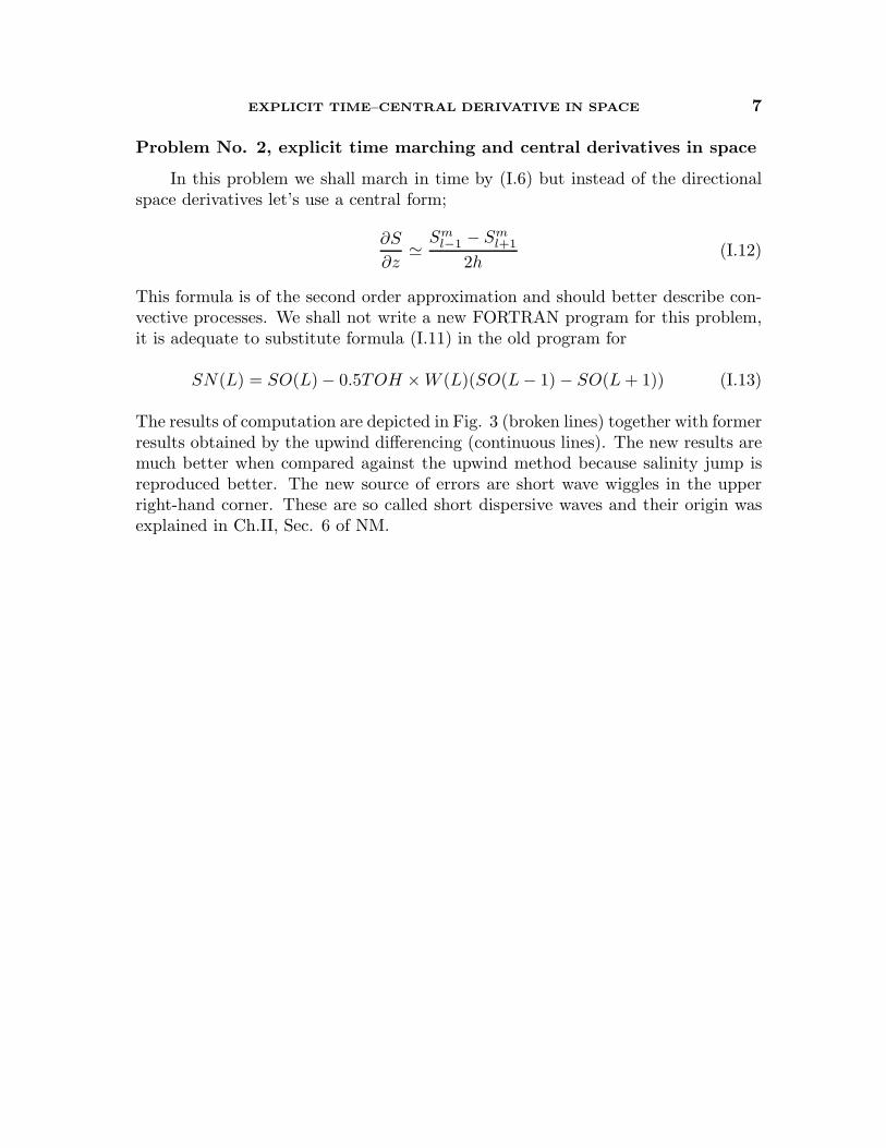
Problem No. 2, explicit time marching and central derivatives in space
In this problem we shall march in time by (I.6) but instead of the directionalspace derivatives let’s use a central form;
∂S
∂z� Sm
l−1 − Sml+1
2h(I.12)
This formula is of the second order approximation and should better describe con-vective processes. We shall not write a new FORTRAN program for this problem,it is adequate to substitute formula (I.11) in the old program for
SN(L) = SO(L) − 0.5TOH ×W (L)(SO(L− 1) − SO(L + 1)) (I.13)
The results of computation are depicted in Fig. 3 (broken lines) together with formerresults obtained by the upwind differencing (continuous lines). The new results aremuch better when compared against the upwind method because salinity jump isreproduced better. The new source of errors are short wave wiggles in the upperright-hand corner. These are so called short dispersive waves and their origin wasexplained in Ch.II, Sec. 6 of NM.
8EX
PLIC
ITT
IME–C
EN
TR
AL
DER
IVAT
IVE
INSPA
CE
Fig.I.3: Central derivative
0 10 20 30 40 50GRID POINTS
0.0
0.2
0.4
0.6
0.8
SA
LIN
ITY
100T 500T 990T
Initial distribution
SIMPLE CORRECTION SCHEMES 9
Problem No. 3, simple correction schemes
Two numerical schemes used for calculation of the convection depict severe lim-itations. Directional derivatives due to numerical diffusion smooth salinity jump,while central derivatives generate parasite short wave spikes which may influencephysics of propagation. For example, these numerical spikes in the vertical distribu-tion of salinity may lead to an unstable density stratification and generate motionrelated rather to numerical than physical causes. In the ensuing consideration thenumerical schemes with better properties will be constructed, but now we demon-strate a very simple scheme for suppressing some of the short wave oscillations. InNM several simple ways of improving performance of the numerical schemes hasbeen delineated. To suppress numerical friction a positive definite scheme (Ch.II,Sec. 9.2) can be used. To partly suppress short wave oscillations numerical scheme(2.257) from NM can be used,
Sm+1l − Sm
l
T+ w
Sml−1 − Sm
l+1
2h
−Aw2T
2h2(Sm
l+1 + Sml−1 − 2Sm
l ) = 0 (I.14)
The last term in this equation serves to suppress short waves. If one comparesformula (I.14) with the original expression (2.257), one finds the coefficient A. Thiscoefficient serve to derive better results and usually A is ranging from 10 to 20.Results of applications of the above scheme with A = 15 are given in Fig.4. Againfor comparison, results of this exercise are depicted together with the results fromthe upwind scheme.

10SIM
PLE
CO
RR
EC
TIO
NSC
HEM
ES
Fig.I.4: Central corrected
0 10 20 30 40 50GRID POINTS
0.0
0.2
0.4
0.6
0.8
SA
LIN
ITY
100T 500T 990T
Initial distribution
QUICKEST METHOD 11
Problem No. 4, QUICKEST method
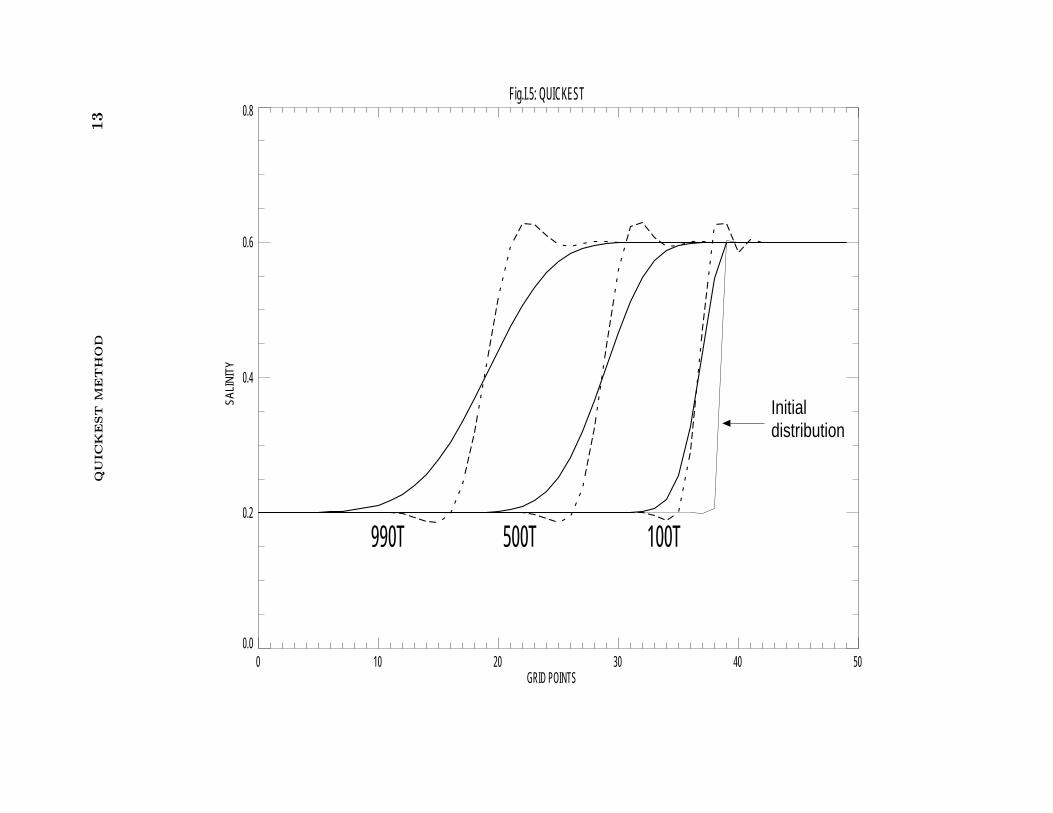
Computational algorithm (I.14) has been constructed with the help of Taylorseries and basic diffusive equation. Derivation is outlined in (2.177) through (2.195).The algorithm is not totally effective but shows improvement. Basic idea is to bringsecond derivative for correction of numerical errors. The QUICKEST (Ch.II, Sec.9.4b of NM) unlike previous methods increases number of grid points around maincomputational point. By using two points upstream and downstream from thecomputational grid point the higher order derivatives are constructed and betterapproximation is achieved. We shall use here formula (2.195) from NM in thespecific geometry related to the vertical coordinate and for the positive verticalvelocity only.
SN(L) = SO(L) −Q ∗ (0.5 ∗ (SO(L− 1) − SO(L + 1))
−0.5 ∗Q ∗ (SO(L + 1) + SO(L− 1) − SO(L) ∗ 2.)
+(SO(L + 2) − 3. ∗ SO(L + 1) + 3. ∗ SO(L)− SO(L− 1)) ∗ (1 −Q ∗Q)/6.) (I.15)
Here Q = wT/H. This nondimensional number is often called Courant number.The program given below (quickest.f) applies the same geometry and parame-
ters as Problem No.1. The result of computation depicted in Fig. 5 (broken lines)is compared against directional derivatives result (continuous lines).
======================================================C PROGRAM TO CALCULATE CONVECTION BY QUICKESTc program quickest.fc program originated by Z.K. at IMSPARAMETER (LZZ=50)REAL W(LZZ),SO(LZZ),SN(LZZ),HZ(LZZ)T=1000. ! time stepMON=1000 ! total number of time stepsDO L=1,LZZHZ(L)=5.END DODO L=1,39SO(L)=0.2END DODO L=40,LZZSO(L)=0.6
12 QUICKEST METHOD
END DOOPEN(UNIT=3,NAME=’SOZ.VER’,STATUS=’UNKNOWN’)C SET VERTICAL VELOCITYDO L=1,LZZ-1W(L)=1.0E-4END DOc q parameter =w*T/hzQ=(1.0E-4)*T/5c start time loop50 N=N+1c write salinity at time step 2,100,500,990.IF(N.EQ.2.OR.N.EQ.100.OR.N.EQ.500.OR.N.EQ.990)THENWRITE(3,*)(SO(L),L=1,LZZ)END IFc calculate new salinityDO L=3,LZZ-2SN(L)=SO(L)-Q*(0.5*(SO(L-1)-SO(L+1))-0.5*Q*(SO(L+1)+SO(L-1)-2SO(L)*2.)+(SO(L+2)-3.*SO(L+1)+3.*SO(L)-SO(L-1))*(1-Q*Q)/6.)END DOc keep two boundary points as known valuesSN(1)=0.2SN(2)=0.2SN(LZZ)=0.6SN(LZZ-1)=0.6C CHANGE VARIABLESDO L=1,LZZSO(L)=SN(L)END DOIF(N.EQ.MON) GO TO 18c return to repeat loopGO TO 5018 CONTINUEEND
QU
ICK
EST
MET
HO
D13
Fig.I.5: QUICKEST
0 10 20 30 40 50GRID POINTS
0.0
0.2
0.4
0.6
0.8
SA
LIN
ITY
100T 500T 990T
Initialdistribution
14 STABILITY PARAMETERS
Problem No. 5, stability parameters.
Among various properties of an numerical algorithm we discuss stability param-eter because it helps to grasp quickly the basic properties of the applied algorithm.
Upwind schemeStarting from the upwind equation in the form (I.10), and searching for stability
of this equation with the help of (2.48) from NM, we obtain stability parameter λin the complex form,
λ = 1 − wT
h+
wT
h(cosκh + i sinκh) (I.16)
Amplitude or absolute value of this parameter defines stability of an upwind nu-merical scheme and for the positive velocity it is given by formula (2.52) from NM,
|λ|2 = 1 + 2q(q − 1)(1 − a) (I.17)
Here: q = wT/h and a = cosκh. As we know |λ| ≤ 1 only if q is less than1. Behavior of the stability parameter depends on two nondimensional numbers q(nondimensional Courant number) and κh. It is obvious that the Courant num-ber describes ratio of convective transport velocity (w) and numerical cell velocity(h/T ). The nondimensional number
κh =2πhL
(I.18)
defines ratio of given wavelength L to the space step h. The shortest possiblewavelength is L = 2h. The wave is usually well resolved in space when L/h ≥ 10.
Stability parameter is a complex number and together with the amplitudeof stability parameter (which we usually call stability parameter), the second in-formation is available, i.e., phase. Stability parameter answers important question,namely how signal is changed due to numerical scheme. The amplitude tells whethera signal over one time step was amplified or damped, the phase tells whether signalwas accelerated or deccelerated. We shall briefly describe this dependence througheq.(I.17) for the stability and for the phase we use the following approach. Accordingto formula (2.49) from NM
λ = c∗eiωT = c∗(cosωT + i sinωT ) (I.19)
The phase lag α can be defined from this formula as
tanα =sinωT
cosωT(I.20)
STABILITY PARAMETERS 15
Comparing (I.16) to the right hand side of (I.19) we arrive at formula for the phaselag of the upwind differencing scheme,
tanα =q sinκh
1 − q(1 − cosκh)(I.21)
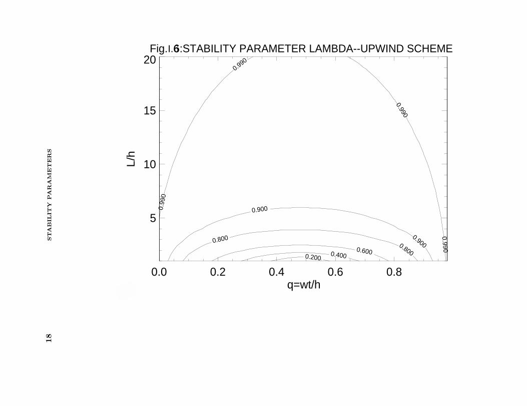
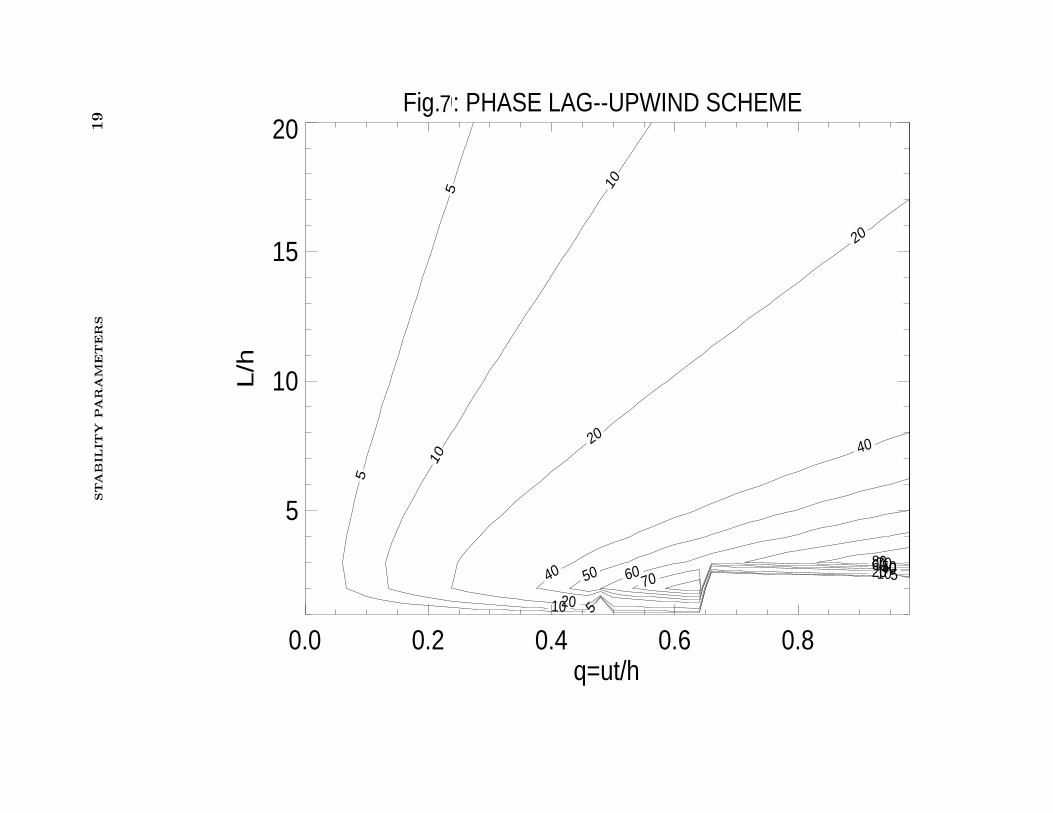
In the ensuing program (stability.f) both stability amplitude and phase lag arecalculated. The result of computations are depicted in Figs. 6 and 7. Errors in thestability and phase are diminishing with the higher spatial resolution. The role ofthe Courant number is less obvious.
Before embarking on the rough road of calculations it is well advised to lookinto properties of (I.17) and (I.21) by considering various values of nondimensionalparameters. For example, behavior of these formulas at the shortest wave resolvedby the numerical grid (L=2h) should always be scrutinized. Thus if L=2h, coskh=-1 and sinkh=0. Therefore |λ|=1, when q=1 or q=0. Clearly tanα=0 at L=2h.Behavior of tanα is also very specific at q=0.5, q=� 0.67 and q=1. At these valuestanα changes sign and the phase in Fig.7 depicts discontinuity. Assume for exampleL=3h, hence κh=2π/3 and (I.21) will change sign at q� 0.67.
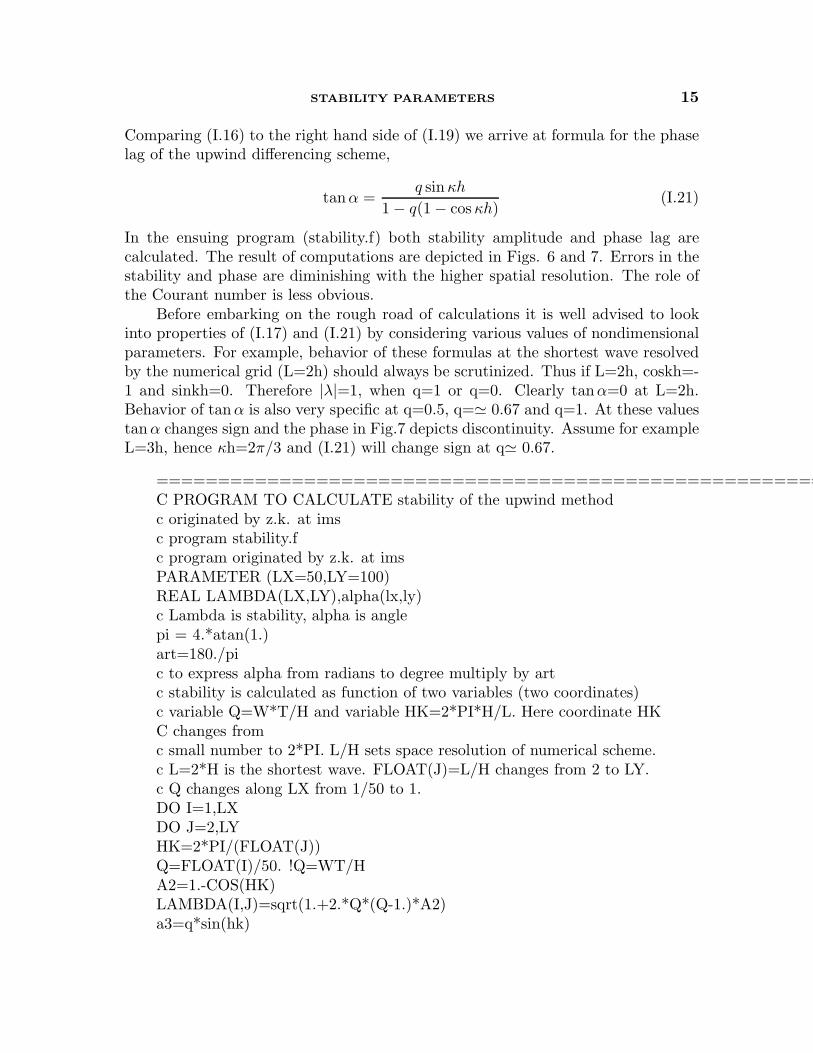
======================================================C PROGRAM TO CALCULATE stability of the upwind methodc originated by z.k. at imsc program stability.fc program originated by z.k. at imsPARAMETER (LX=50,LY=100)REAL LAMBDA(LX,LY),alpha(lx,ly)c Lambda is stability, alpha is anglepi = 4.*atan(1.)art=180./pic to express alpha from radians to degree multiply by artc stability is calculated as function of two variables (two coordinates)c variable Q=W*T/H and variable HK=2*PI*H/L. Here coordinate HKC changes fromc small number to 2*PI. L/H sets space resolution of numerical scheme.c L=2*H is the shortest wave. FLOAT(J)=L/H changes from 2 to LY.c Q changes along LX from 1/50 to 1.DO I=1,LXDO J=2,LYHK=2*PI/(FLOAT(J))Q=FLOAT(I)/50. !Q=WT/HA2=1.-COS(HK)LAMBDA(I,J)=sqrt(1.+2.*Q*(Q-1.)*A2)a3=q*sin(hk)
16 STABILITY PARAMETERS
a4=-q*a2+1.a5=a3/(a4+1.0E-6)alpha(i,j)=art*(atan(a5))END DOEND DOopen (unit=12,file=’lambda.dat’,status=’unknown’)open (unit=13,file=’phase.dat’,status=’unknown’)write(12,*)((lambda(j,k),j=1,lx),k=1,ly)write(13,*)((alpha(j,k),j=1,lx),k=1,ly)END
STABILITY PARAMETERS 17
Central space derivative and forward time derivative (CF).
Let us check stability properties of the numerical scheme used in theproblem No.2 and based on (I.6) and (I.12). Again using (2.48) from NM, we
arrive atλ− 1T
=iw
hsinκh (I.22)
Stability parameter is|λ| =
[1 + (q sinκh)2
]1/2 (I.23)
In this formula q = wT/h. From the above formula follows that the stabilityparameter is always greater than one, and therefore numerical scheme is unstable.If we check again Problem No.2 we can see that indeed the amplitude of the shortwaves in Fig.3 is increasing in time.
Central space derivative and central time derivative (CC).
Instead using forward derivative in time we shall use central derivative in thefollowing scheme
Sm+1l − Sm−1
l
2T= −w
Sml−1 − Sm
l+1
2h(I.24)
This is scheme is also given in NM as (2.60). Before we check stability properties of(I.24) a few comments are needed on organization of computation by this formula.To march in time we need to know S on two previous time step (l and l−1). If onlyone initial condition is given the best way to start is to use forward derivative intime. After this first step the time marching can be done by the leapfrog explainedin Fig. 3.5 of NM.
Searching stability of (I.24) we obtain two roots for the stability parameter(this result is close to (2.61) from NM),
λ1,2 =iq1 ±
√4 − q2
1
2(I.25)
Here q = 2wTh , q1 = q sinκh. When q2
1 ≤ 4 or wTh ≤ 1, stability parameter |λ| = 1,
and numerical scheme is stable. Although amplitude of the signal is not altered bynumerical scheme the phase of the signal undergoes change defined by,
tanα =q sinκh√
4 − (q sinκh)2(I.26)
The resulting phase lag is given in Fig.8.
18STA
BIL
ITY
PA
RA
MET
ER
SFig.I.6:STABILITY PARAMETER LAMBDA--UPWIND SCHEME
0.0 0.2 0.4 0.6 0.8q=wt/h
5
10
15
20
L/h
0.2000.400
0.6000.800
0.800 0.900
0.900
0.990
0.990
0.990
0.99
0
6
I.6
STA
BIL
ITY
PA
RA
MET
ER
S19
Fig.9: PHASE LAG--UPWIND SCHEME
0.0 0.2 0.4 0.6 0.8q=ut/h
5
10
15
20
L/h
55
5
5
10
10
10
10
20
20
20
20
4040
40
5050 60
607080
70
7

20STA
BIL
ITY
PA
RA
MET
ER
SFig.I.8: PHASE LAG--CENTRAL SCHEME
0.0 0.2 0.4 0.6 0.8q=wt/h
5
10
15
20
L/h
55
5
5
1010
10
20
20
20
40
40
5060
70

FLUX FORM OF CONVECTIVE TRANSPORT 21
2. Flux form of convective/advective transport
Here we shortly describe an upstream-downstream numerical schemes employ-ing equation of transport in the flux form. Such an equation is based on the princi-ple of flux conservation. The difference equations constructed from the differentialequations should as well display the same conservative properties. We shall searchfor the schemes which will possess good accuracy, so that they will introduce smallamplitude and phase errors. Also we shall search for the schemes which are positivedefinite to avoid instabilities due to parasitic short waves.
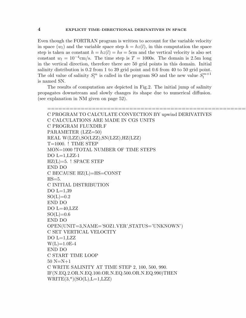
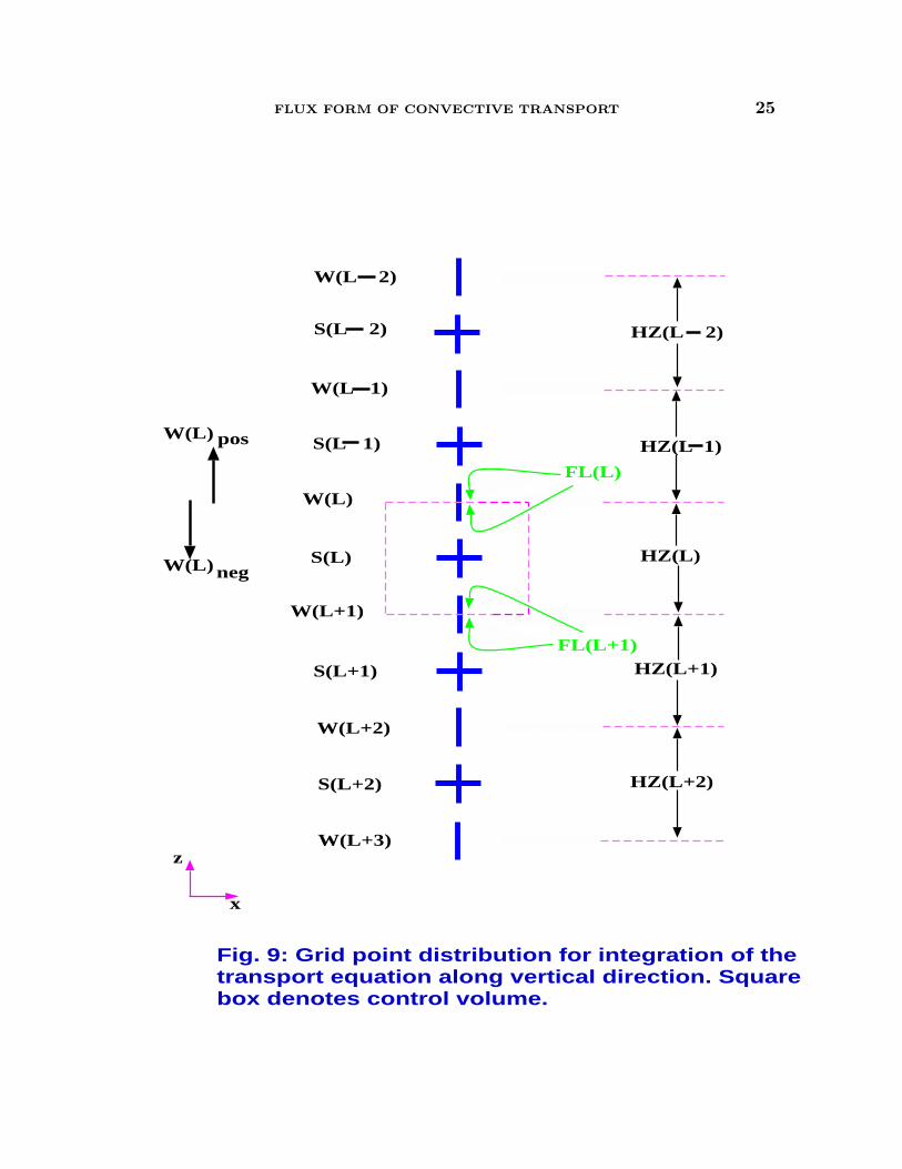
Let’s start from upstream-downstream scheme. Consider a control surfacespanned around concentration grid point S(L) – Fig.9
Square box (red dash lines) denotes control surface. Crosses are located at theconcentration points S, and vertical bars denote w component of velocity. The griddistance HZ is variable and is measured between the vertical velocity grid points.
Let us integrate equation of transport for salinity
∂S
∂t+
∂wS
∂z= 0 (I.27)
over a region dz and time dt, then
∫ T
0
(∫ ∆z
0
∂S
∂tdz)dt = −
∫ T
0
(∫ ∆z
0
∂wS
∂zdz)dt (I.28)
The left hand side term is easily transformed into a finite difference form. Theintegral on the right hand side is transformed into an integral along the boundaryof the control surface. Thus
(Sm+1l − Sm
l )∆z = −[(wS)mU − (wS)mD ]T (I.29)
or dividing by ∆z and T we arrive at the familiar finite difference form
Sm+1l − Sm
l
T= −(wS)mU − (wS)mD
∆z(I.30)
It remains to express fluxes through the surfaces as functions of velocity on thesurfaces. Thus defining the positive and negative velocity at the upper surface ofthe control volume which spans the grid point S(L) (see Fig.9),
wpU = 0.5(|wm
l | + wml ); wn
U = 0.5(−|wml | + wm
l ), (I.31)
the flux at the upper surface can be expressed in the upstream- downstream form
(wS)mU = wpUSm
l + wnUSm
l−1 (I.32)
22 FLUX FORM OF CONVECTIVE TRANSPORT
Similar approach can be used to define fluxes at the lower surface. Again the positiveand negative velocity can be written as,
wpD = 0.5(|wm
l+1| + wml+1); wn
D = 0.5(−|wml+1| + wm
l+1), (I.33)
and afterwards flux through the surface follows,
(wS)mD = wpDSm
l+1 + wnDSm
l (I.34)
Eqs. (I.32) and (I.34) shows that the formulas for the flux at the upper and lowersurface are very similar, and it is sufficient to change index in eqs. (I.31) and (I.32)from l to l+1 to derive eq. (I.34). Therefore, in ensuing consideration we shall onlydevelop formulas for the upper surface of the control volume.
Now, from eq. (I.30) the updated value of salinity can be calculated by thefollowing finite difference form
Sm+1l − Sm
l
T= −(wS)mU − (wS)mD
∆z= −(wS)mU − (wS)mD
HZ(l)
= −FL(l) − FL(l + 1)HZ(l)
(I.35)
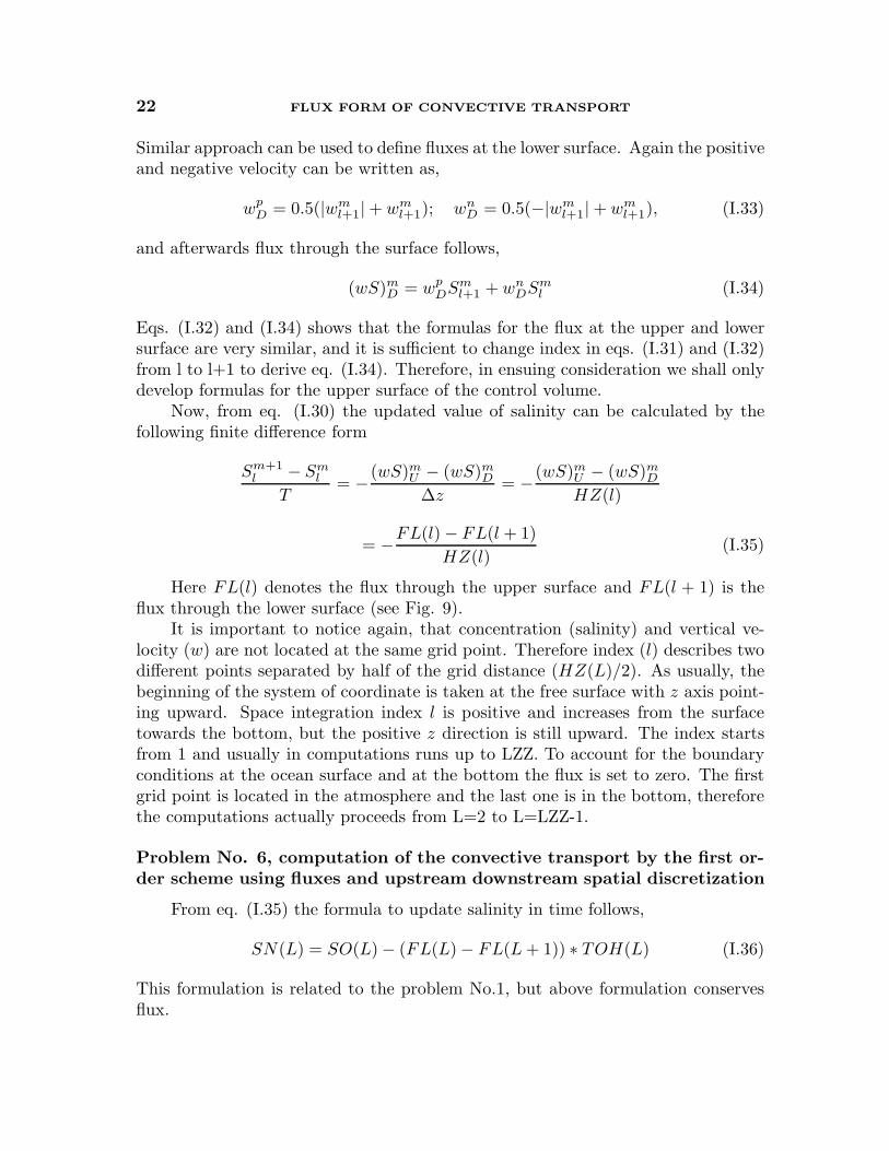
Here FL(l) denotes the flux through the upper surface and FL(l + 1) is theflux through the lower surface (see Fig. 9).
It is important to notice again, that concentration (salinity) and vertical ve-locity (w) are not located at the same grid point. Therefore index (l) describes twodifferent points separated by half of the grid distance (HZ(L)/2). As usually, thebeginning of the system of coordinate is taken at the free surface with z axis point-ing upward. Space integration index l is positive and increases from the surfacetowards the bottom, but the positive z direction is still upward. The index startsfrom 1 and usually in computations runs up to LZZ. To account for the boundaryconditions at the ocean surface and at the bottom the flux is set to zero. The firstgrid point is located in the atmosphere and the last one is in the bottom, thereforethe computations actually proceeds from L=2 to L=LZZ-1.
Problem No. 6, computation of the convective transport by the first or-der scheme using fluxes and upstream downstream spatial discretization
From eq. (I.35) the formula to update salinity in time follows,
SN(L) = SO(L) − (FL(L) − FL(L + 1)) ∗ TOH(L) (I.36)
This formulation is related to the problem No.1, but above formulation conservesflux.
FLUX FORM OF CONVECTIVE TRANSPORT 23
Beneath the FORTRAN program (FLUXDDIR.F) is written to account for thevariable velocity in space (wl) and the variable space step HZ(L). The time stepis T = 1000s. There are 100 grid points in this domain. Initial salinity distributionis 0.6 from 1 to 49 grid point and 0.2 from 50 to 100 grid point. The old value ofsalinity Sm
l is called in the program SO and the new value Sm+1l is named SN. The
velocity is constant and is set to −1.0 × 10⁻⁴.
C PROGRAM TO CALCULATE CONVECTION BY Fluxes using upstreamC DERIVATIVES PROGRAM FLUXDDIR.FPARAMETER (LZZ=100)REAL W(LZZ),SO(LZZ),SN(LZZ),HZ(LZZ),TOH(LZZ)REAL FL(LZZ)T=1000. ! TIME STEPMON=1000 !TOTAL NUMBER OF TIME STEPSDO L=1,LZZHZ(L)=5.-2.5*L/lzz ! SPACE STEP is variableTOH(L)=T/HZ(L) ! COMBINATION OF TIME STEP AND SPACE STEPEND DOC INITIAL DISTRIBUTION of salinityDO L=1,49SO(L)=0.6END DODO L=50,LZZSO(L)=0.2END DOOPEN(UNIT=3,NAME=’SOZ1.VER’,STATUS=’UKNOWN’)C SET VERTICAL VELOCITYDO L=1,LZZW(L)=-1.0E-4END DOC START TIME LOOP50 N=N+1C WRITE SALINITY AT TIME STEP 1, 100, 500, 990.IF(N.EQ.1.OR.N.EQ.100.OR.N.EQ.500.OR.N.EQ.990)THENWRITE(3,*)(SO(L),L=1,LZZ)END IFC CALCULATE NEW VALUE OF flux FLFL(2)=0. ! FLUX AT SURFACEFL(LZZ)=0. ! FLUX AT BOTTOMDO L=3,LZZ-1wpL=0.5*(w(l)+abs(w(l))) ! POSITIVE VELOCITYwnL=0.5*(w(l)-abs(w(l))) ! NEGATIVE VELOCITY

24 FLUX FORM OF CONVECTIVE TRANSPORT
FL(L)=WPL*SO(L)+WNL*SO(L-1) ! FLUX THROUGH UPPER SURFACEEND DOC NEW SALINITY SNDO L=2,LZZ-1SN(L)=SO(L)-(FL(L)-FL(L+1))*TOH(L)END DOC KEEP BOUNDARY VALUESSN(LZZ-1)=0.2SN(2)=0.6C BOUNDARY CONDITIONS SET EQUAL SALINITY AT TWO POINTSC SO THAT THE FLUX IS ZERO AT THE BOUNDARIES.sN(LZZ)=SN(LZZ-1)SN(1)=SN(2)C CHANGE VARIABLESDO L=1,LZZSO(L)=SN(L)END DOC STOP COMPUTATION AT TIME STEP MONIF(N.EQ.MON) GO TO 18C RETURN BACK TO 50 TO REPEAT TIME LOOPGO TO 5018 CONTINUEEND
The results of computation are depicted are exactly the same as in Fig. 2.Initial jump of salinity propagates downstream and slowly changes its shape due tonumerical diffusion. (see explanation in NM given on page 52).
FLUX FORM OF CONVECTIVE TRANSPORT 25
HZ(L)
HZ(L 1)
HZ(L 2)
HZ(L+1)
HZ(L+2)
W(L)
S(L)
W(L+1)
S(L 1)
W(L 1)
S(L 2)
W(L 2)
S(L+1)
W(L+2)
S(L+2)
W(L+3)
W(L) pos
W(L) neg
FL(L)
FL(L+1)
z
x
Fig. 9: Grid point distribution for integration of the transport equation along vertical direction. Squarebox denotes control volume.

26 FLUX FORM OF CONVECTIVE TRANSPORT
Problem No. 7, computation of the convection by second order schemeusing fluxes and upstream downstream spatial discretization
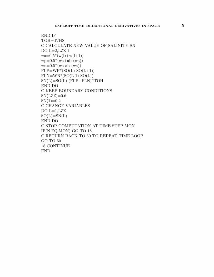
A forward in time upstream convection/advection scheme described above isbased on conservative principle and well preserves positivity. Unfortunately, it alsodisplay strong numerical dissipation, hence the sharp front in the salinity distribu-tion at the initial time becomes smoothed in the process of computation. To derivehigher order schemes we continue to use the upstream approach. The flux at thecell’s boundary will be defined by the salinity which will be derived through linearand polynomial fitting. In the upstream formulation of eq. (I.27) for the positivevelocity it is assumed that flux of salinity through the upper surface carries thevalue of salinity from the nearest point S(L). For the negative velocity the flux isbased on salinity S(L-1). To increase order of approximation one needs to knowthese values at the future time preferably at time step m+1/2. For this purposethemethod of characteristics will be used. Equation (I.27) has such property that S isconstant along any line defined by z−wt = const. Let w(L) is positive velocity andtime step is T. The value of salinity which is at the distance Tw from the uppersurface of the cell will be the future value of salinity at the upper surface after timestep T elapses. To predict value of salinity for the half time step the distance shouldbe 0.5Tw. Thus the approach is straightforward: approximate linearly the value ofsalinity at the distance 0.5T(w(L) + |w(L)|) from the upper surface for the positivevelocity and at the distance 0.5T(w(L)−|w(L)|) for the negative velocity (Fig. 10).Salinity at the upper surface for the positive velocity (Sm+1/2
UP ) is
Sm+1/2UP =
S(L)[0.5HZ(L− 1) + 0.5Tw(L)] + S(L− 1)[0.5HZ(L) − 0.5Tw(L)]0.5[HZ(L− 1) + HZ(L)]
(I.37)Similar approach can be used to define salinity at the upper surface for the
negative velocity (Sm+1/2UN )
Sm+1/2UN =
S(L)[0.5HZ(L− 1) + 0.5Tw(L)] + S(L− 1)[0.5HZ(L) − 0.5Tw(L)]0.5[HZ(L− 1) + HZ(L)]
(I.38)The salt flux through the upper surface can be expressed similarly to eq. (I.32)
FLm+1/2(L) = (wS)m+1/2U = wp
USm+1/2UP + wn
USm+1/2UN (I.39)
To obtain flux at the lower surface of the control volume it is sufficient tochange index L in the above formula to L + 1 and define velocities at the lowersurface accordingly to eq. (I.33). New value of salinity at the L grid point can nowbe defined based on the new flux formulation
Sm+1l − Sm
l
T= −(wS)m+1/2
U − (wS)m+1/2D
∆z= −(wS)m+1/2
U − (wS)m+1/2D
HZ(l)
FLUX FORM OF CONVECTIVE TRANSPORT 27
= −FLm+1/2(l) − FLm+1/2(l + 1)HZ(l)
(I.40)
From eq. (I.40) the formula to update salinity in time follows,
SN(L) = SO(L) − (FL(L) − FL(L + 1)) ∗ TOH(L) (I.41)
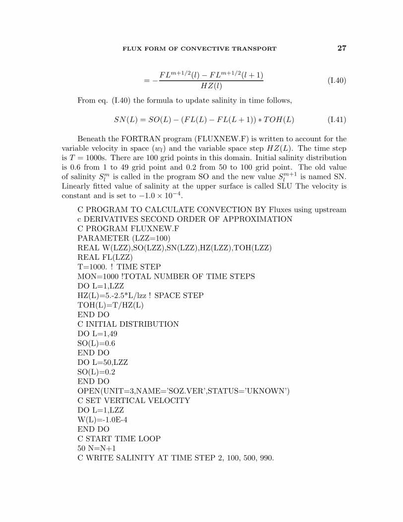
Beneath the FORTRAN program (FLUXNEW.F) is written to account for thevariable velocity in space (wl) and the variable space step HZ(L). The time stepis T = 1000s. There are 100 grid points in this domain. Initial salinity distributionis 0.6 from 1 to 49 grid point and 0.2 from 50 to 100 grid point. The old valueof salinity Sm
l is called in the program SO and the new value Sm+1l is named SN.
Linearly fitted value of salinity at the upper surface is called SLU The velocity isconstant and is set to −1.0 × 10⁻⁴.
C PROGRAM TO CALCULATE CONVECTION BY Fluxes using upstreamc DERIVATIVES SECOND ORDER OF APPROXIMATIONC PROGRAM FLUXNEW.FPARAMETER (LZZ=100)REAL W(LZZ),SO(LZZ),SN(LZZ),HZ(LZZ),TOH(LZZ)REAL FL(LZZ)T=1000. ! TIME STEPMON=1000 !TOTAL NUMBER OF TIME STEPSDO L=1,LZZHZ(L)=5.-2.5*L/lzz ! SPACE STEPTOH(L)=T/HZ(L)END DOC INITIAL DISTRIBUTIONDO L=1,49SO(L)=0.6END DODO L=50,LZZSO(L)=0.2END DOOPEN(UNIT=3,NAME=’SOZ.VER’,STATUS=’UKNOWN’)C SET VERTICAL VELOCITYDO L=1,LZZW(L)=-1.0E-4END DOC START TIME LOOP50 N=N+1C WRITE SALINITY AT TIME STEP 2, 100, 500, 990.

28 FLUX FORM OF CONVECTIVE TRANSPORT
IF(N.EQ.1.OR.N.EQ.100.OR.N.EQ.500.OR.N.EQ.990)THENWRITE(3,*)(SO(L),L=1,LZZ)END IFc TOH=T/HSC CALCULATE NEW VALUE OF SALINITY SNFL(2)=0.FL(LZZ)=0.DO L=3,LZZ-1C LINEAR APPROXIMATION OF SALINITY AT THE UPPER SURFACE
OF A CONTROL VOLUMEHSU=0.5*(HZ(L)+HZ(L-1))wpL=0.5*(w(l)+abs(w(l)))wnL=0.5*(w(l)-abs(w(l)))SLU1=0.5*(HZ(L-1)+W(L)*T)*SO(L)SLU2=0.5*(HZ(L)-W(L)*T)*SO(L-1)SLU=(SLU1+SLU2)/HSUFL(L)=(WPL*SLU+WNL*SLU)END DODO L=2,LZZ-1SN(L)=SO(L)-(FL(L)-FL(L+1))*TOH(L)END DOC KEEP BOUNDARY CONDITIONSSN(LZZ-1)=0.2SN(2)=0.6SN(LZZ)=0.2SN(1)=0.6C CHANGE VARIABLESDO L=1,LZZSO(L)=SN(L)END DOC STOP COMPUTATION AT TIME STEP MONIF(N.EQ.MON) GO TO 18C RETURN BACK TO 50 TO REPEAT TIME LOOPGO TO 5018 CONTINUEEND
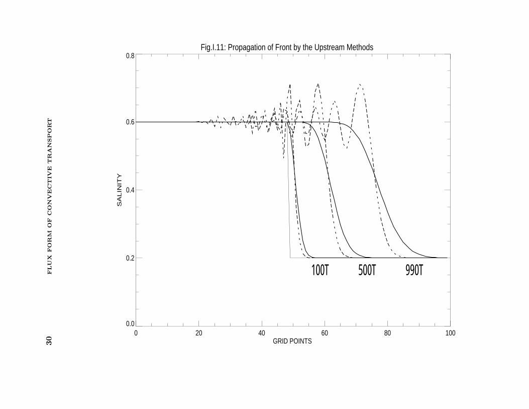
The computed salinity distribution is depicted in Fig.11. Broken lines depictsolution by the first order method and continuous lines by the second order method.Although the second order method reproduces front much better in comparison tothe first order method it does generate parasitic short waves which appear to growin time.

FLUX FORM OF CONVECTIVE TRANSPORT 29
HZ(L 2)
HZ(L+2)
W(L)
S(L)
W(L+1)
S(L 1)
W(L 1)
S(L 2)
W(L 2)
S(L+1)
W(L+2)
S(L+2)
W(L+3)
W(L) pos
W(L) neg
FL(L)
FL(L+1)
z
x
HZ(L)
HZ(L 1)
HZ(L+1)
0.5TW(L)pos
0.5TW(L)neg
z
x
Fig. 10: Grid point distribution for integration of the transport equation by the second order scheme usingupstream/downstream spatial discretization.
30FLU
XFO
RM
OF
CO
NV
EC
TIV
ET
RA
NSP
ORT
Fig.I.11: Propagation of Front by the Upstream Methods
0 20 40 60 80 100GRID POINTS
0.0
0.2
0.4
0.6
0.8
SA
LIN
ITY
100T 500T 990T
FLUX FORM OF CONVECTIVE TRANSPORT 31
Problem No. 8, computation of the convection by third order schemeusing fluxes and upstream downstream spatial discretization
Second order scheme developed above shows improvement over the first orderscheme, therefore we shall continue along this approach by fitting better approxima-tion to the concentration at the surface of the control volume. For this purpose anupstream-biased stencil of three concentration points will be used. For the positivevelocity at the upper surface three salinity points, namely: S(l-1), S(l) and S(l+1)are used to predict salinity for the half time step ahead at the upper surface (Fig.9). Since this salinity at time step m is located at the distance 0.5Tw(l) from theupper surface of the control volume (Fig. 10), one can use the three above men-tioned grid points to fit salinity at this location. A Lagrangian polynomial will befit to this discrete set of data. The general form of three point polynomial can bewritten in the following way,
Sm+1/2UP = P2,0Sl+1 + P2,1Sl + P2,2Sl−1 (I.42)
Here
P2,0 =(z − z1)(z − z2)
(z0 − z1)(z0 − z2)
P2,1 =(z − z0)(z − z2)
(z1 − z0)(z1 − z2)
P2,2 =(z − z0)(z − z1)
(z2 − z0)(z2 − z1)(I.43)
To relate this general formula to our geometry a local system of coordinate isintroduced. Beginning of this system is set at the S(l+1) grid point. Thus z0 = 0,z1 = 0.5(HZ(l + 1) + HZ(l)) and z2 = z1 + 0.5(HZ(l) + HZ(l − 1)). Variabledistance z = z1 + 0.5(HZ(l) − w(l)T ).
For the negative velocity at the upper surface the upstream-biased stencil isbased on S(l), S(l-1) and S(l-2) grid points (Figs. 9 and 10). Thus salinity due tothe negative velocity at the upper surface is defined as,
Sm+1/2UN = P2,0Sl + P2,1Sl−1 + P2,2Sl−2 (I.44)
Here Lagrangian polynomial is again defined by the general formula eq. (I.42), butthe coefficients will follow from the new (local) coordinate system. This time thebeginning is chosen at the point S(l) and z0 = 0, z1 = 0.5(HZ(l) + HZ(l− 1)) andz2 = z1 + 0.5(HZ(l− 1) + HZ(l − 2)). Variable distance z = 0.5(HZ(l) − w(l)T ).
Using these new expressions the salt flux through the upper surface can bestipulated similarly to eq. (I.32),
FLm+1/2(L) = (wS)m+1/2U = wp
USm+1/2UP + wn
USm+1/2UN (I.45)
32 FLUX FORM OF CONVECTIVE TRANSPORT
To obtain flux at the lower surface of the control volume it is sufficient to changeindex L in the formulas for the upper surface to L + 1 and define velocities at thelower surface accordingly to eq. (I.33). Temporal change of salinity at the L gridpoint can now be defined based on this new flux formulation
Sm+1l − Sm
l
T= −(wS)m+1/2
U − (wS)m+1/2D
∆z= −(wS)m+1/2
U − (wS)m+1/2D
HZ(l)
= −FLm+1/2(l) − FLm+1/2(l + 1)HZ(l)
(I.46)
From eq. (I.46) the updated salinity follows,
SN(L) = SO(L) − (FL(L) − FL(L + 1)) ∗ TOH(L) (I.47)
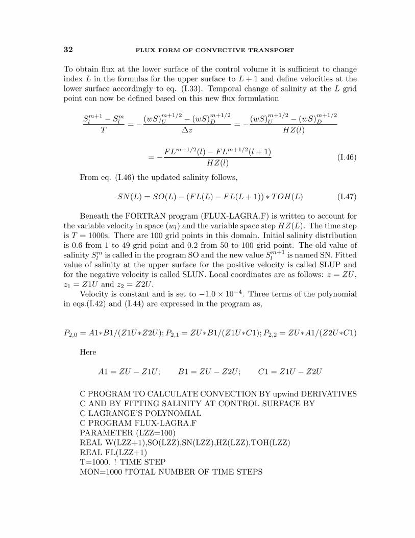
Beneath the FORTRAN program (FLUX-LAGRA.F) is written to account forthe variable velocity in space (wl) and the variable space step HZ(L). The time stepis T = 1000s. There are 100 grid points in this domain. Initial salinity distributionis 0.6 from 1 to 49 grid point and 0.2 from 50 to 100 grid point. The old value ofsalinity Sm
l is called in the program SO and the new value Sm+1l is named SN. Fitted
value of salinity at the upper surface for the positive velocity is called SLUP andfor the negative velocity is called SLUN. Local coordinates are as follows: z = ZU ,z1 = Z1U and z2 = Z2U .
Velocity is constant and is set to −1.0 × 10⁻⁴. Three terms of the polynomialin eqs.(I.42) and (I.44) are expressed in the program as,
P2,0 = A1∗B1/(Z1U∗Z2U);P2,1 = ZU∗B1/(Z1U∗C1);P2,2 = ZU∗A1/(Z2U∗C1)
Here
A1 = ZU − Z1U ; B1 = ZU − Z2U ; C1 = Z1U − Z2U
C PROGRAM TO CALCULATE CONVECTION BY upwind DERIVATIVESC AND BY FITTING SALINITY AT CONTROL SURFACE BYC LAGRANGE’S POLYNOMIALC PROGRAM FLUX-LAGRA.FPARAMETER (LZZ=100)REAL W(LZZ+1),SO(LZZ),SN(LZZ),HZ(LZZ),TOH(LZZ)REAL FL(LZZ+1)T=1000. ! TIME STEPMON=1000 !TOTAL NUMBER OF TIME STEPS

FLUX FORM OF CONVECTIVE TRANSPORT 33
DO L=1,LZZHZ(L)=5.-2.5*L/lzz ! SPACE STEPTOH(L)=T/HZ(L)END DOC BECAUSE HZ(L)=HS=CONSTc HS=5.C INITIAL DISTRIBUTIONDO L=1,49SO(L)=0.6END DODO L=50,LZZSO(L)=0.2END DOOPEN(UNIT=3,NAME=’SOZ1.VER’,STATUS=’UKNOWN’)C SET VERTICAL VELOCITYDO L=1,LZZW(L)=-1.0E-4END DOC START TIME LOOP50 N=N+1C WRITE SALINITY AT TIME STEP 2, 100, 500, 990.IF(N.EQ.1.OR.N.EQ.100.OR.N.EQ.500.OR.N.EQ.990)THENWRITE(3,*)(SO(L),L=1,LZZ)END IFC CALCULATE NEW VALUE OF SALINITY SN.C FLUX AT L=1 AND LZZ+1 IS 0.FL(2)=0FL(LZZ)=0DO L=3,LZZ-1WPU=.5*(W(L)+ABS(W(L)))WNU=.5*(W(L)-ABS(W(L)))c positive velocity at upper boundaryc beggining of local coordinate for lagrange polynomialc at z=hz(l+1)/2=0C Z=ZU, Z1=Z1U; Z2=Z2Uz1u=0.5*(HZ(L)+HZ(L+1))Z2U=0.5*(HZ(L)+HZ(L+1))+HZ(L)ZU=HZ(L)+0.5*(HZ(L+1)-WPU*T)A1=ZU-Z1UB1=ZU-Z2UC1=Z1U-Z2USLU1=SO(L+1)*A1*B1/(Z1U*Z2U)
34 FLUX FORM OF CONVECTIVE TRANSPORT
SLU2=SO(L)*ZU*B1/(Z1U*C1)SLU3=-SO(L-1)*ZU*A1/(Z2U*C1)SLUP=SLU1+SLU2+SLU3z1u=0.5*(HZ(L)+HZ(L-1))Z2U=0.5*(HZ(L)+HZ(L-2))+HZ(L-1)ZU=0.5*(HZ(L)-WNU*T)A1=ZU-Z1UB1=ZU-Z2UC1=Z1U-Z2USLU1=SO(L)*A1*B1/(Z1U*Z2U)SLU2=SO(L-1)*ZU*B1/(Z1U*C1)SLU3=-SO(L-2)*ZU*A1/(Z2U*C1)SLUN=SLU1+SLU2+SLU3c positive velocity at lower boundaryc beggining of local coordinate for lagrange polynomialc at z=hz(l+2)/2 =0FL(L)=WPU*SLUP+WNU*SLUNEND DOdo l=2,LZZ-1SN(L)=SO(L)-(FL(L)-FL(L+1))*TOH(L)end doC KEEP BOUNDARY CONDITIONSSN(LZZ-1)=0.2 ! this conditions to keep value 0.2 at the rightc side otherwise concentration at the right side will grow because fluxc through the boundary is zero. (this comment for negative velocity)SN(2)=0.6 ! otherwise 0.6 will travel away and 0 will start toc generate.C BELOW NEED TO KEEP OUTSIDE SALINITY EQUAL TO INSIDE
SALINITYsN(LZZ)=SN(LZZ-1)SN(1)=SN(2)C CHANGE VARIABLESDO L=1,LZZSO(L)=SN(L)END DOC STOP COMPUTATION AT TIME STEP MONIF(N.EQ.MON) GO TO 18C RETURN BACK TO 50 TO REPEAT TIME LOOPGO TO 5018 CONTINUEEND
FLUX FORM OF CONVECTIVE TRANSPORT 35
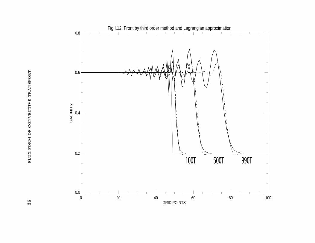
The result of computations are given in Fig.12 for the second-order (continuousline) and for the third order (broken lines). Two improvements can be noticed, thefront is better reproduced and short wave oscillations have been limited to one spikewhose amplitude is constant in time.
36FLU
XFO
RM
OF
CO
NV
EC
TIV
ET
RA
NSP
ORT
Fig.I.12: Front by third order method and Lagrangian approximation
0 20 40 60 80 100GRID POINTS
0.0
0.2
0.4
0.6
0.8
SA
LIN
ITY
100T 500T 990T
FLUX FORM OF CONVECTIVE TRANSPORT 37
Problem No. 9, computation of advection by the third order schemeusing fluxes and the upstream/downstream spatial discretization (geom-etry along x direction).
A second order scheme are written for the geometry along the vertical direc-tion (index of integration is diminishing along positive z direction). In the regulargeometry an index of enumeration is increased along the positive direction. Aboveformulas we will rewrite along x axis. Let consider the flux through the right surfaceof a control volume. For the positive velocity at the right-hand surface the threesalinity points, namely: S(j-1), S(j) and S(j+1) are used to predict salinity whichwill occur half time step later at the right-hand surface. Since this salinity at thetime step m is located at the distance 0.5Tu(j+1) from the surface, the three abovementioned grid points can be used to fit salinity at this location. A Lagrangianpolynomial will be fit to this discrete set of data.
Sm+1/2RP = P2,0Sj−1 + P2,1Sj + P2,2Sj+1 (I.48)
Here
P2,0 =(x− x1)(x− x2)
(x0 − x1)(x0 − x2)
P2,1 =(x− x0)(x− x2)
(x1 − x0)(x1 − x2)
P2,2 =(x− x0)(x− x1)
(x2 − x0)(x2 − x1)(I.49)
To relate this general formula to our geometry a local system of coordinate isintroduced. Beginning of this system is set at the S(j-1) grid point. Thus x0 = 0,x1 = HX and x2 = 2HX . Variable distance x = x1 + 0.5(HX − u(j + 1)T ). Herewe assume that the space step of numerical integration along x direction is constantand equal to HX .
For the negative velocity at the right-hand surface the upstream-biased stencilis based on S(j), S(j+1) and S(J+2) grid points. Thus salinity due to negativevelocity at the right hand surface is defined as,
Sm+1/2RN = P2,0Sj + P2,1Sj+1 + P2,2Sj+2 (I.50)
Here Lagrangian polynomial is again defined by the general formula eq.(I.42),but the coefficients will follow from the new local coordinate system. This time,the beginning is chosen at the point S(j) and x0 = 0, x1 = HX and x2 = 2HX .Variable distance x = 0.5(HX − u(j + 1)T ). Using these new expressions the saltflux through the right-hand surface can be stipulated similarly to eq. (I.32),
FLm+1/2(j + 1) = (uS)m+1/2R = upRS
m+1/2RP + unRS
m+1/2RN (I.51)
38 FLUX FORM OF CONVECTIVE TRANSPORT
To obtain flux at the left-hand surface of the control volume it is sufficient tochange index j in the formulas for the righ-hand surface to j−1 and define velocitiesat the left-hand surface.
New value of salinity at the j grid point can now be defined based on the newflux formulation
Sm+1j − Sm
j
T= −(uS)m+1/2
R − (uS)m+1/2L
∆x= −(uS)m+1/2
R − (uS)m+1/2L
HX
= −FLm+1/2(j + 1) − FLm+1/2(j)HX
(I.52)
From eq. (I.52) formula to update salinity follows,
SN(j) = SO(j) − (FL(j + 1) − FL(j)) ∗ T/HX (I.53)
We will not construct FORTRAN program to compute advection because pro-gram (FLUX-LAGRA.F) can be easily adapted for this task.
Problem No. 10, computation of convection by Flux-Corrected Method(FCT)
The flux–corrected method is well described in the Ch.II, Sec. 9.5. It is appliedinfrequently in the large oceanic models because it needs a few step to achieve result.These steps when repeated many times in the large models make big difference inthe computer time required for solving problems.
The main portion of the FCT is limiter or filter which produces ripple-freesolution. The limiter is given by eq.(2.213) from NM. It works by limiting an an-tidifusive flux, i.e., flux which is a difference of the two fluxes, obtained by two dif-ferent method. One method is the low order method (usually related to directionalderivatives), and second method is the high order method. The latter reproduceswell salinity jump but produces also dispersive short waves. In the NM the highorder numerical schemes in time are based on the symmetrical central derivative.Here we use the high accuracy the third order scheme.
The FCT algorithm constructs the net fluxes point by point as a weightedaverage of a low-order scheme and a high-order scheme. This weighting is done insuch manner as to maximize the use of the high order scheme without overshootingor undershooting. The FCT algorithm can be broken down into six steps.
1. Compute FLl – flux by the low order scheme. The purpose here is to derive
a positive definite, or sometimes called monotonic, solution. For our purpose it isonly important that the monotonic solution is ripple-free. Solution is obtained bythe method of upstream discretization described by eqs. (I.31) –(I.35)
FLUX FORM OF CONVECTIVE TRANSPORT 39
2. Compute FHl – flux by the high order scheme. Here the third order approx-
imation given by eqs.(I.37)–(I.40) is used.3. Introduce an antidiffusive flux as
Al = FHl − FL
l (I.54)
4. Compute low order updated solution (SL)
SLm+1l = Sm
l − T
h(FL
l − FLl+1) (I.55)
5. Limit antidiffusion fluxes in such a way that the new concentration (Sm+1)is ripple-free. This is accomplished through limiter Ll as
ALl = LlAl, 0 ≤ Ll ≤ 1 (I.56)
6. Use the limited antidiffusive flux to derive concentration Sm+1l
Sm+1l = SLm+1
l − T
h(AL
l − ALl+1) (I.57)
In the construction of the finite-difference formulas we use the staggered grid de-picted in Fig. 9.
Basic formulas for the low order and high order solution were constructedabove. Below is given Fortran program fluxall.f. New value of salinity calculatedby the low order scheme is called SNL. Flux obtained by the low order scheme isdenoted as FLL and flux calculated by the high order scheme is FL. Antidiffusiveflux is AUN.
C PROGRAM TO CALCULATE CONVECTION BY Flux Corrected MethodC PROGRAM FLUXALL.FPARAMETER (LZZ=100)REAL W(LZZ),SO(LZZ),SN(LZZ),SNL(LZZ),HZ(LZZ),TOH(LZZ)REAL FLL(LZZ),FL(LZZ),AU(LZZ)REAL TOH1(LZZ)T=1000. ! TIME STEPMON=1000 !TOTAL NUMBER OF TIME STEPSDO L=1,LZZHZ(L)=5.-2.5*L/lzz ! SPACE STEPTOH(L)=T/HZ(L)TOH1(L)=0.5*(HZ(L)+HZ(L-1))/TEND DOC INITIAL DISTRIBUTIONDO L=1,49
40 FLUX FORM OF CONVECTIVE TRANSPORT
SO(L)=0.6END DODO L=50,LZZSO(L)=0.2END DOOPEN(UNIT=3,NAME=’SOZ1.VER’,STATUS=’UKNOWN’)C SET VERTICAL VELOCITYDO L=1,LZZW(L)=-1.0E-4END DOC START TIME LOOP50 N=N+1C WRITE SALINITY AT TIME STEP 1, 100, 500, 990.IF(N.EQ.1.OR.N.EQ.100.OR.N.EQ.500.OR.N.EQ.990)THENWRITE(3,*)(SO(L),L=1,LZZ)END IFc TOH=T/HSC CALCULATE NEW VALUE OF SALINITY SN BY THE LOW ORDER
SCHEMEFLL(LZZ)=0.DO L=2,LZZ-1WPU=.5*(W(L)+ABS(W(L)))WNU=.5*(W(L)-ABS(W(L)))FLL(L)=WPU*SO(L)+WNU*SO(L-1)END DODO L=2,LZZ-1SNL(L)=SO(L)-(FLL(L)-FLL(L+1))*TOH(L)END DOFL(2)=0.FL(LZZ)=0.DO L=3,LZZ-1WPU=.5*(W(L)+ABS(W(L)))WNU=.5*(W(L)-ABS(W(L)))c positive velocity at upper boundaryc beggining of local coordinate for lagrange polynomialc at z=hz(l+1)/2=0z1u=0.5*(HZ(L)+HZ(L+1))Z2U=0.5*(HZ(L)+HZ(L+1))+HZ(L)ZU=HZ(L)+0.5*(HZ(L+1)-WPU*T)A1=ZU-Z1UB1=ZU-Z2UC1=Z1U-Z2U
FLUX FORM OF CONVECTIVE TRANSPORT 41
SLU1=SO(L+1)*A1*B1/(Z1U*Z2U)SLU2=SO(L)*ZU*B1/(Z1U*C1)SLU3=-SO(L-1)*ZU*A1/(Z2U*C1)SLUP=SLU1+SLU2+SLU3C NEGATIVE VELOCITY AT UPPER BOUNDARYc beggining of local coordinate for lagrange polynomialC AT THE POINT C(L),Z=0z1u=0.5*(HZ(L)+HZ(L-1))Z2U=0.5*(HZ(L)+HZ(L-2))+HZ(L-1)ZU=0.5*(HZ(L)-WNU*T)A1=ZU-Z1UB1=ZU-Z2UC1=Z1U-Z2USLU1=SO(L)*A1*B1/(Z1U*Z2U)SLU2=SO(L-1)*ZU*B1/(Z1U*C1)SLU3=-SO(L-2)*ZU*A1/(Z2U*C1)SLUN=SLU1+SLU2+SLU3FL(L)=WPU*SLUP+WNU*SLUNC INTRODUCE ANTIDIFFUSIVE FLUXC AT UPPER SURFACEAUN=FL(L)-FLL(L)C FILTERING FIKU-MIKUA0=AUNA1=SIGN(1.0,A0)A2=A1*(SNL(L-2)-SNL(L-1))*TOH1(L-1)A3=A1*(SNL(L)-SNL(L+1))*TOH1(L+1)A4=ABS(AUN)A5=AMIN1(A2,A3,A4)AU(L)=A1*AMAX1(0.,A5)END DOAU(2)=0.AU(LZZ)=0.C NEW SALINITYDO L=2,LZZ-1SN(L)=SNL(L)-(AU(L)-AU(L+1))*TOH(L)END DOC KEEP BOUNDARY CONDITIONSSN(LZZ)=0.2SN(LZZ-1)=0.2SN(1)=0.6SN(2)=0.6

42FLU
XFO
RM
OF
CO
NV
EC
TIV
ET
RA
NSP
ORT
Fig.I.13: Front by upstream third order method and FCT
0 20 40 60 80 100GRID POINTS
0.0
0.2
0.4
0.6
0.8
SA
LIN
ITY
100T 500T 990T

FLUX FORM OF CONVECTIVE TRANSPORT 43
C CHANGE VARIABLESDO L=1,LZZSO(L)=SN(L)END DOC STOP COMPUTATION AT TIME STEP MONIF(N.EQ.MON) GO TO 18C RETURN BACK TO 50 TO REPEAT TIME LOOPGO TO 5018 CONTINUEENDThe result of calculation by FCT (broken lines) and by third order scheme
(continuous line) is given in Fig. 12. The FCT produced output without anyparasitic waves.

44 FLUX FORM OF CONVECTIVE TRANSPORT
PROPAGATION IN CHANNEL 45
CHAPTER II
TWO-DIMENSIONAL MODELS
1. Propagation in channel
We shall construct numerical algorithms for two dimensional problems de-scribed in the first part of Ch.III of NM. In order to identify the important steps inthe constructing and analysis of a numerical scheme we shall consider first propaga-tion of the long wave in a channel. These experiments are described in the Ch.III,Sec.3 of NM.
We shall consider the numerical solution of the equations of motion and conti-nuity
∂u
∂t= −g
∂ζ
∂x(II.1)
∂ζ
∂t= − ∂
∂x(Hu) (II.2)
Solution of this system is usually searched by the two-time-level or by the three-time-level numerical schemes. For construction of the space derivatives in the equa-tions (II.1) and (II.2), a space staggered grid (Figure 3.2 from NM) is usually used(Arakawa C grid). The two-time-level numerical scheme (3.46 from NM)
(um+1j − umj )
T= −g
ζmj − ζmj−1
h(II.3)
ζm+1j − ζmj
T= −(um+1
j+1 Hj+1 − um+1j Hj)
h(II.4)
is of the second order of approximation in space and only the first order intime. For the quick reference we shall call above the Fisher’s scheme. The leapfrog(three-time-level scheme)
(um+1j − um−1
j )2T
= −gζmj − ζmj−1
h(II.5)
ζm+1j − ζm−1
j
2T= −(umj+1Hj+1 − umj Hj)
h(II.6)
46 PROPAGATION IN CHANNEL
is of the second order of approximation in time and space.The space-staggered grid given in Figure 3.2 from NM is used to construct the
space derivatives in the above equations. The variables u and ζ are located in sucha way that the second order of approximation in space is achieved. The depth istaken in the sea level points. The space step along the x direction is h. Index mstands for the time stepping. In the Fisher scheme the time step is T and in theleapfrog scheme the time step is 2T . To demonstrate a distortion generated by thefinite difference equations due to an approximation error, let us consider a simplecase of a sinusoidal wave propagating over a long distance in the channel of constantdepth. At the left end of the channel a sinusoidal wave is given as
ζ = ζ0 sin(2πtTp
) (II.7)
Here the amplitude is ζ0=100 cm, and the period is Tp=10 min. Propagation ofthis monochromatic wave toward the right end of the channel will be reproduced.The right end is open, and a radiating condition will be used so that the wave canpropagate beyond the channel without reflection (eq. 3.45 from NM). At the leftend of the channel (II.7) is applied for one period only; after that, the radiatingcondition is used as well. The channel is 2100 km long and 4077 m deep. The waveperiod under consideration is 10 min, which results in a 120-km wavelength. Thetime step of numerical integration will be taken in all experiments equal to 10 s.The space step is chosen equal to 12 km. The 12-km space grid sets 10 steps perwavelength (SPW). Such a resolution introduces numerical errors resulting in thewave dispersion.
Problem No. 1, solution by Fisher method
We start by solving above problem through the method given by the set ofequations (II.3) and (II.4). The name of program is FISHER.F. Time step (T) is10s and space step (DX) is equal to 12km. Therefore in the channel of 2100 kmlength there are 175 grid points. Two variables are considered namely sea level (Z- old value; ZN - new value), and velocity (U old value; UN new value). Spaceindex is j, it runs from j=1 to j=je. At the left-hand open boundary a sinusoidalwave of 100 cm amplitude is given as: zn(1)=100.*sin(0.1047197*float(mo-1)). Inthis formula mo denotes index of time stepping. At the right-hand end of channela radiating condition is used to calculate velocity. First, the new velocity UN iscomputed. After computing the new value of velocity, this value is introducedinto the sea level computations because of stability considerations. The change ofvariables in loop 14 actually performs time stepping in which the new values becomethe old ones. Command GO TO 50 brings the whole process to the beginning ofthe time loop and the computations can be repeated again until mo=mon.
C Program fisher.f
PROPAGATION IN CHANNEL 47
C PROGRAM COMPUTE propagation in 1D channelC by fisher method (eq. 3.46 from NM)C program originated by Z.K. at IMS, AlaskaPARAMETER (je=175)REAL U(je),UN(je),Z(je),ZN(je) ! Velocity and sea levelREAL H(je),H1(JE) ! Depth and total depthopen (unit=10,file=’euler.dat’,status=’unknown’)c mon is total number of time stepsmon=1001c if B=1 total depth is computed H1=H+ZB=0.G=982.c time step and space stept=10.DX=12.e5 ! grid step in cmC COEFFICIENTS FOR EQUATIONSPL=2.0*T/DXPLG=G*PLc depthdo j=1,jeh1(j)=4.077e5h(j)=h1(j)end doc start time loop50 MO=MO+1leu=leu+1c input boundary for one period and afterwards radiating conditionzn(1)=-u(2)*sqrt(h(2)/g) ! Sea level from radiation conditionif(mo.gt.60)go to 22zn(1)=100.*sin(0.1047197*float(mo-1)) ! Sea levl given for the 60C time steps22 continuec radiating boundary at the very end of the channelUn(je)=Z(je-1)*SQRT(G/H(je-1))C compute velocityDO80 J=2,je-1UN(J)=U(J)-.5*PLG*(Z(J)-Z(J-1))80 CONTINUEc compute sea levelDO 120 J=2,je-1ZN(J)=Z(J)+.5*PL*(UN(J)*(H1(J)+H1(J-1))/2.0-UN(J+12)*(H1(J+1)+H1(J))/2.)

48 PROPAGATION IN CHANNEL
120 CONTINUEC CHANGE OLD VARIABLES TO NEWDO 14 J=1,jeU(J)=UN(J)H1(J)=H(J)+B*(ZN(J))Z(J)=ZN(J)14 CONTINUEif(mo.eq.60.or.mo.eq.360.or.mo.eq.670.or.mo.eq.980)thenprint *, mowrite (10,*)(zn(j),j=1,je-1)end ifIF(MO.EQ.MON)GO TO 23 ! Finish computationsGO TO 5023 CONTINUEEND
Problem No. 2, solution by leap-frog method
Now we solve the same problem by the leapfrog method described by eqs. (II.5)and (II.6). First we note that the time stepping is done through three time levels,therefore we introduce additional time level called respectively UO for the velocity,and ZO for the sea level. To begin computations in time by the leapfrog methodtwo initial conditions are needed. One way to resolve this problem is to use atwo-time-level numerical scheme to derive one additional initial value. Therefore,in the program we have constructed below, both leapfrog and Fisher method areused. Fisher scheme is used not only for generating an additional initial condition.Leapfrog scheme may generate two solutions. One of these is parasite solutionwhich can obfuscate physical solution (see Ch.II. Sec.7 in NM). In a simple caseof the constant depth, we consider here, the parasite solution is not present. Itcan be damped by calling Fisher scheme every 20 time steps or so. This optionis built in the program LEAPFROG.F. All other notations are from the programfisher.f. One thing to remember is to scrutinize Fig. 3.5 from NM before startingcomputations. Although the leapfrog method requires double time step, due tochange of the variables, the time stepping in the leapfrog and in the Fisher methodis the same (see how old and intermediate variables are upgraded to the new onesin the loop 14 of the below program).
c program: leapfrog.fC PROGRAM COMPUTES propagation in 1D channelc by leap-frog methodC program originated by Z.K. at IMS, AlaskaPARAMETER (je=175)C
PROPAGATION IN CHANNEL 49
REAL U(je),UN(je),Z(je),ZN(je)REAL H(je),UO(je),ZO(je),H1(JE)open (unit=10,file=’lp10c5.dat’,status=’unknown’)C B SERVE TO CONTROL TOTAL DEPTHC IF B=1.,TOTAL DEPTH H1=H+B*(Z+TE)B=0.mon=1001c basic dataG=982.c time step and space stept=10.DX=12.e5c depthdo j=1,jeh1(j)=4.077e5h(j)=h1(j)end doPL=2.0*T/DX ! notice double time stepc start time loop50 MO=MO+1leu=leu+1c input boundary only for one period and then switch toc radiating condirionzn(1)=-u(2)*sqrt(h(2)/g)if(mo.gt.60)go to 22zn(1)=100.*sin(0.1047197*float(mo-1))22 continuec radiating boundary at the very end of the channelUn(je)=Z(je-1)*SQRT(G/H(je-1))C TO INITIALIZE COMPUTATION USE FISHER SCHEMEC OR MAY BE YOU WISH TO APPLYC IT EVRY 20 STEPS TO REMOVE NON-PHYSICAL SOLUTION.C FOR THIS PURPOSE COUNTER LEU IS INTRODUCEDc if(leu.eq.20)go to 99 ! For Fisher’s restartc IF(MO.EQ.1.or.mo.gt.1)GO TO 99IF(MO.EQ.1)GO TO 99C LEAP-FROGDO8 J=2,je-1c calculate velocityUN(J)=UO(J)-PL*G*(Z(J)-Z(J-1))8 CONTINUEDO 12 J=2,je-1
50 PROPAGATION IN CHANNEL
ump=0.5*u(j)*(h1(j)+h1(j-1))up1=0.5*u(j+1)*(h1(j)+h1(j+1))C CALCULATE SEA LEVELZN(J)=ZO(J)+PL*(ump-up1)12 CONTINUEC========================================C FISHER RESTARTGO TO 98 ! Skip Fisher99 LEU=0C CALCULATE VELOCITYDO80 J=2,je-1UN(J)=U(J)-.5*PL*G*(Z(J)-Z(J-1))80 CONTINUEC CALCULATE SEA LEVELDO 120 J=2,je-1ZN(J)=Z(J)+.5*PL*(UN(J)*(H1(J)+H1(J-1))/2.0-UN(J+12)*(H1(J+1)+H1(J))/2.)120 CONTINUE98 CONTINUEC CHANGE OLD VARIABLES TO NEWDO 14 J=1,jeUO(J)=U(J)U(J)=UN(J)H1(J)=H(J)+B*(ZN(J))ZO(J)=Z(J)Z(J)=ZN(J)14 CONTINUEif(mo.eq.60.or.mo.eq.360.or.mo.eq.670.or.mo.eq.980)thenprint *, mowrite (10,*)(zn(j),j=1,je-1)end ifc stop calculation when mo=monIF(MO.EQ.MON)GO TO 23GO TO 5023 CONTINUEEND
The results of computations derived by the Fisher and leapfrog algorithms aredepicted in Fig.II.1. In both solutions the wave propagating from the left end dis-plays diminishing amplitude along the channel. It has also a tail of secondary wavesfollowing the main wave. These distortions are due to the numerical approxima-tions we applied. In the governing equations (II.1) and (II.2) there is no friction or
PROPAGATION IN CHANNEL 51
dispersion responsible for the results given in Fig.II.1. Comparing the upper andlower part of Fig.II.1 one can see that solutions are quite similar. Because leapfroghas second order approximation in time and Fisher’s scheme is only of the firstorder, one can conclude that distortions seen in Fig.II.1 are due mainly to the spaceresolution.

52P
RO
PA
GAT
ION
INC
HA
NN
EL
0 500 1000 1500 2000DISTANCE IN KILOMETERS
-100
-50
0
50
100
LE
VE
L(C
M)
Fig.II.1: WAVE PROPAGATION IN CHANNEL
0 500 1000 1500 2000-100
-50
0
50
100
LE
VE
L(C
M)
Fisher
Leap-Frog
PROPAGATION IN CHANNEL 53
Problem No. 3, solution by corrected leap-frog method
To find the terms responsible for wave distortion in the leapfrog method, weshall introduce the Taylor series (see Ch.II of NM) into (II.5)and (II.6), to obtain
∂u
∂t+
T 2
6∂3u
∂t3= −g(
∂ζ
∂x+
124
∂3ζ
∂x3h2) + O(h4, T 4) (II.8)
∂ζ
∂t+
T 2
6∂3ζ
∂t3= −∂(uH)
∂x− 1
24∂3(uH)∂x3
h2 + O(h4, T 4) (II.9)
Thus the terms that introduce wave distortion are dependent on the thirdderivatives in space and time. Having written explicitly the error of approximation,we may correct this error by introducing its value into (II.5) and (II.6) with anopposite sign. Here we briefly describe the way to calculate space derivatives bydefining a numerical form of a third derivative of the sea level in the u point,
∂3ζ
∂x3� −ζj−2 + 3ζj−1 − 3ζj + ζj+1
h3(II.10)
The time derivatives are calculated somewhat differently as
∂3ζ
∂t3� 0.5ζm+2
j − ζm+1j + ζm−1
j − 0.5ζm−2j
T 3(II.11)
The following correction will be introduced into the leapfrog scheme of (II.5)and (II.6).
Ctu =T 2
6∂3u
∂t3Cxu =
124
∂3ζ
∂x3h2 (II.12)
Ctζ =T 2
6∂3ζ
∂t3Cxζ =
124
∂3(uH)∂x3
h2 (II.13)
These corrections written in the numerical form can be introduced into system(II.5) and (II.6) with the opposite signs,
(um+1j − um−1
j )2T
− Ctum = −gζmj − ζmj−1
h+ gCxζm (II.14)
ζm+1j − ζm−1
j
2T− Ctζm = −(umj+1Hj+1 − umj Hj)
h+ Cxum (II.15)
Direct application of this approach leads to mixed results: the spatial correctionworks well, while the temporal correction leads to the unstable numerical scheme.This time behavior of the leapfrog numerical scheme is caused by the presence ofthe so-called false solution. Therefore we direct our attention to redefining the time

54 PROPAGATION IN CHANNEL
derivative in such a way that it will not influence overall stability of the numericalscheme. For construction of the third derivative in time, we shall change timederivative into the space derivative. From (II.1) and (II.2)
∂3u
∂t3= −g2
[∂2H
∂x2
∂ζ
∂x+ 2
∂H
∂x
∂2ζ
∂x2+ H
∂3ζ
∂x3
](II.16)
∂3ζ
∂t3= −g
[∂H
∂x
∂uH
∂x+ H
∂3uH
∂x3
](II.17)
At this point, we introduce further simplification by assuming a flat bottom so thedepth derivative in the above equations will vanish. Thus (II.8) and (II.9) by using(II.16)) and (II.17) changes to:
∂u
∂t= −g
∂ζ
∂x− g(
h2x
24− gH
T 2
6)∂3ζ
∂x3h2 + O(h4, T 4) (II.18)
∂ζ
∂t= −∂uH
∂x
−(h2x
24− gH
T 2
6)∂3uH
∂x3h2 + O(h4, T 4) (II.19)
Having written explicitly the error of approximation, we may correct this erroras in the system (II.14)-(II.15).
The leapfrog program with these corrections is called SIMPDISP.F. Notationis similar to the programs given above and the new addition is related to to thehigher order terms. Because it is difficult to define third derivative in the end pointsof the channel the coefficients ai, and aii are introduced to account for this problem
c program: simpdisp.fC PROGRAM COMPUTES propagation in 1D channelc by leap-frog methodc additional corrections are put on/off by commenting orc uncommenting d2 in loop 8 and d4 in loop 12.C program originated by Z.K. at IMS, AlaskaPARAMETER (je=175)CREAL U(je),UN(je),Z(je),ZN(je)REAL H(je),UO(je),ai(je),aii(je)REAL ZO(je),H1(JE)open (unit=10,file=’lp10c5.dat’,status=’unknown’)C B SERVE TO CONTROL TOTAL DEPTHC IF B=1.,TOTAL DEPTH H1=H+B*(Z+TE)B=0.
PROPAGATION IN CHANNEL 55
mon=1001c basic dataG=982.c time step and space stept=10.DX=12.e5c depthdo j=1,jeh1(j)=4.077e5h(j)=h1(j)end doPL=2.0*T/DXDX2=DX*DXDX3=DX*DX*DXpd=2.*T/(DX3)c this is done to for correction in proximity to the boundarydo j=1,jeai(j)=0.aii(j)=0.end dodo j=3,je-3ai(j)=1end dodo j=5,je-5aii(j)=1end doc start time loop50 MO=MO+1leu=leu+1c input boundary only for one period and then switch toc radiating condirionzn(1)=-u(2)*sqrt(h(2)/g)if(mo.gt.60)go to 22zn(1)=100.*sin(0.1047197*float(mo-1))22 continuec radiating boundary at the very end of the channelUn(je)=Z(je-1)*SQRT(G/H(je-1))C TO INITIALIZE COMPUTATION USE FISHER SCHEME OR MAYC BE YOU WISH TO APPLYC IT EVRY 20 STEPS TO REMOVE NON-PHYSICAL SOLUTION.C FOR THIS PURPOSE COUNTER LEU IS INTRODUCEDc if(leu.eq.20)go to 99
56 PROPAGATION IN CHANNEL
c IF(MO.EQ.1.or.mo.gt.1)GO TO 99IF(MO.EQ.1)GO TO 99C LEAP-FROGDO8 J=2,je-1HS=.5*(H1(J)+H1(J-1))c numerical dispersion correctionc comment line d2=0 for correctiond1=-ai(j)*pd*G*(T*T*g*hs/6.-DX2/24.)d2=d1*(z(j+1)-3.*z(j)+3.*z(j-1)-z(j-2))d11=aii(j)*pL*G/(1920.)d21=d11*(z(j+2)-5.*z(j+1)+10.*z(j)-10*z(j-1)+5.*z(j-2)-z(j-3))d2=d2+d21d2=0.c calculate velocityUN(J)=UO(J)-PL*G*(Z(J)-Z(J-1))+d28 CONTINUEDO 12 J=2,je-1um2=0.5*u(j-2)*(h1(j-3)+h1(j-2))um1=0.5*u(j-1)*(h1(j-2)+h1(j-1))ump=0.5*u(j)*(h1(j)+h1(j-1))up1=0.5*u(j+1)*(h1(j)+h1(j+1))up2=0.5*u(j+2)*(h1(j+2)+h1(j+1))up3=0.5*u(j+3)*(h1(j+3)+h1(j+2))HS=.5*(H1(J)+H1(J-1))c numerical dispersion correction,c comment line d4=0 for correctiond3=-ai(j)*pd*(T*T*g*hs/6.-DX2/24.)d4=d3*(up2-3.*up1+3.*ump-um1)d33=aii(j)*pl/(1920.)d31=d33*(up3-5.*up2+10.*up1-10*ump+5.*um1-um2)d4=d4+d31d4=0.C CALCULATE SEA LEVELZN(J)=ZO(J)+PL*(ump-up1)+d412 CONTINUEC===================================C FISHER RESTARTGO TO 9899 LEU=0C CALCULATE VELOCITYDO80 J=2,je-1UN(J)=U(J)-.5*PL*G*(Z(J)-Z(J-1))
PROPAGATION IN CHANNEL 57
80 CONTINUEC CALCULATE SEA LEVELDO 120 J=2,je-1ZN(J)=Z(J)+.5*PL*(UN(J)*(H1(J)+H1(J-1))/2.0-UN(J+12)*(H1(J+1)+H1(J))/2.)120 CONTINUE98 CONTINUEC CHANGE OLD VARIABLES TO NEWDO 14 J=1,jeUO(J)=U(J)U(J)=UN(J)H1(J)=H(J)+B*(ZN(J))ZO(J)=Z(J)Z(J)=ZN(J)14 CONTINUEif(mo.eq.60.or.mo.eq.360.or.mo.eq.670.or.mo.eq.980)thenprint *, mowrite (10,*)(zn(j),j=1,je-1)end ifc stop calculation when mo=monIF(MO.EQ.MON)GO TO 23GO TO 5023 CONTINUEENDThe experiments are performed with a 12-km space step. In every experiment
the equations are first solved without the third derivatives, and subsequently thecorrection is introduced by reversing the sign at the third derivative in (II.18) and(II.19). In Figure II.2 (top part) the results are given for the 12-km grid step(SPW=10). The leapfrog grossly distorts the wave 2000 km from the entrance.The leading wave is no longer dominating the wave pattern. The second wave hasthe largest amplitude, and the trailing waves are significantly modified both in phaseand amplitude owing to energy flow toward the trailing edge. The correction (lowerpart of Fig. II.2) improves the wave parameters and reestablishes the first wave asthe leading wave with 80% original amplitude.

58P
RO
PA
GAT
ION
INC
HA
NN
EL
0 500 1000 1500 2000DISTANCE IN KILOMETERS
-100
-50
0
50
100
LE
VE
L(C
M)
Fig.II.2: WAVE PROPAGATION IN CHANNEL
0 500 1000 1500 2000-100
-50
0
50
100
LE
VE
L(C
M)
Leap -Frog
Leap-Frog-Corrected
NUMERICAL STABILITY 59
Problem No. 4, numerical stability
Here, we shortly discuss stability properties of the numerical scheme givenby (3.47) from NM, (in this chapter equations are numbered as (II.3 and II.4)).Stability parameter of this numerical scheme is always equal to one if Courant-Friedrichs-Lewy condition, √
gH ≤ h
T(II.20)
is fulfilled. To estimate phase lag error introduced by the numerical scheme theformula (3.63) from NM is used.
φ = arctan
√(4Q−Q2)(2 −Q)
(II.21)
Here Q is nondimensional parameter,
Q = 4gH(T
hsin
κh
2)2 (II.22)
which is expressed through the two nondimensional numbers, namely Courant num-ber and spatial resolution number,
T
h
√gH and
L
h(II.23)
We also introduce celerity ratio, as a parameter for the verification of thenumerical scheme approximation (and also its stability). It compares numericallyderived velocity against analytical expression for the phase velocity. The purposeis to retain this parameter close to unity so that the long wave phase velocity inmodel and in nature will have the same value. Celerity ratio is defined by (3.64)from NM, as,
Celerity ratio = cn/ca (II.24)
Here, numerical and analytical celerity is
cn =ω
κ=
φ
κT; ca =
√gH (II.25)
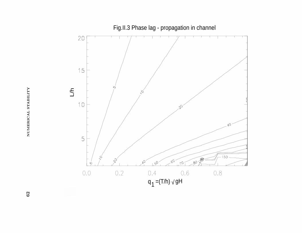
In the ensuing program (stabilitychannel.f) both the phase and celerity ratio arecomputed. To differentiate between notation for the depth and space step, thehorizontal space step is called DX in the program. The results of computations aredepicted in Figs. II.3 and II.4. The basic parameter which can rapidly influencethe phase and celerity ratio is the space resolution. Increasing space resolution willdiminish phase lag and bring celerity ration to unity. Decreasing of the Courantparameter influences phase lag but practically has no influence over celerity ratio.
60 NUMERICAL STABILITY
Small domain at the right lower corner of the figures is influenced by negative valuesof the phase lag and celerity ratio greater than one.
=====================================================C PROGRAM TO CALCULATE stability of the Fisher methodc program stabilitychannel.f (stabilt.f0)c program originated by z.k. at imsPARAMETER (LX=50,LY=100)REAL alpha(lx,ly),Celerity(lx,ly)c alpha is angle , celerity defines ratio of numerical and analyticalc velocitiespi = 4.*atan(1.)art=180./pic to express alpha from radians to degree multiply by artc stability parameter of the Fisher method is equal to unityc ( formula 3.53 from NM) underc condition (3.54a) from NM. Here we calculate phase lag (LAMBDA)c by (3.63) from NM and celerity ratio by (3.64) from NM. Both arec calculated as function of two variables (two coordinates)c variable Q1=sqrt(gH)*T/DX and variable HK=2*PI*DX/L. Here coordinatec HK changes from small number to PI. Here DX denotes space stepc usually in book given as h. L/DX sets horizontal space resolutionc of numerical scheme. L=2*DX is the shortest wave.c FLOAT(J)=L/DX changes from 2 to LY. Q1 changes along LX from 1/50 to
1.DO I=2,LXDO J=1,LYHK=2.*PI/(FLOAT(J))Q1=FLOAT(I)/50. !Q1=sqrt(gH)*T/DXA2=4.*Q1*Q1hk1=hk/2.A3=sin(HK1)*sin(HK1)q=A2*A3a3=4*q-q*qa4=2.-qa5=sqrt(a3)/a4alpha(i,j)=art*(atan(a5))c this is for negative anglesif(alpha(i,j).lt.0.)thenalpha(i,j)=90+abs(alpha(i,j))end ifCelerity(i,j)=alpha(i,j)/(hk*q1*art)END DO

NUMERICAL STABILITY 61
END DOopen (unit=12,file=’celerity.dat’,status=’unknown’)open (unit=13,file=’phasechan.dat’,status=’unknown’)write(12,*)((Celerity(j,k),j=1,lx),k=1,ly)write(13,*)((alpha(j,k),j=1,lx),k=1,ly)stopend
62N
UM
ER
ICA
LSTA
BIL
ITY
13
Fig.II.3 Phase lag - propagation in channel
L/h
q =(T/h) √ gH1

NU
MER
ICA
LSTA
BIL
ITY
63
L/h
q = T/h √gH1
Fig.II.4 Celerity ratio - propagation in channel
64 PROPAGATION IN UPSLOPING CHANNEL
2. Run-up in channel
We shall proceed to construct a simple algorithm for the run-up in the channel.This tool can be easily applied to the 2-D problems with the help of material fromCh.III, Sec.7.1 and 7.2 of NM. Consider equation of motion and continuity along xdirection:
∂u
∂t+ u
∂u
∂x= −g
∂ζ
∂x− ru|u|
D(II.26)
∂ζ
∂t=
∂
∂x(Du) (II.27)
Solution of this system will be searched through the two-time-level numeri-cal scheme. The nonlinear (advective) term will be approximated by the up-wind/downwind scheme. D in the above equations denotes total depth D = H + ζ.The major problem arises when wave starts to move into and out of the dry do-main. Obviously none of the second order symmetrical space schemes can not beused, because the movement is defined only in the wet domain. One of the ma-jor new assumptions is that equation of continuity can be approximated by theupwind/downwind approach as well. This approach makes equation of continuityquite stable at the boundary between wet and dry domains. To simulate run-upand run-down, the variable domain of integration is established after every timestep by checking whether total depth is positive (condition 3.160 from NM). Thefollowing numerical scheme is used to march in time:
(um+1j − umj )
T+ up
(umj − umj−1)h
+ un(umj+1 − umj )
h
= −g(ζmj − ζmj−1)
h+
rumj |umj |0.5(Dm
j + Dmj−1)
(II.28)
Here: up = 0.5(umj + |umj |), and un = 0.5(umj − |umj |)
ζm+1j − ζmj
T= −(upj1 ×Dm
j + unj1 ×Dmj+1 − upj ×Dm
j−1 − unj ×Dmj ) (II.29)
In the above equation:
upj1 = 0.5(um+1j+1 + |um+1
j+1 |) and unj1 = 0.5(um+1j+1 − |um+1
j+1 |)
upj = 0.5(um+1j + |um+1
j |) and unj = 0.5(um+1j − |um+1
j |)The space-staggered grid given in Figure 3.18 from NM is used to construct thespace derivatives and to visualize procedures at the wet/dry boundary. At the leftend of the channel a sinusoidal wave is given:
ζ = ζ0 sin(2πtTp
) (II.30)

PROPAGATION IN UPSLOPING CHANNEL 65
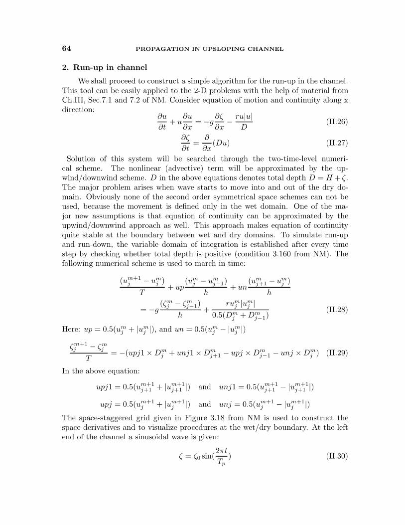
Here the wave period Tp = 1000s. The wave propagates in the channel of 2km long.The bottom of the channel is sloping into the beach. The depth changes linearlyfrom 10m at the left end of the channel to -10m at the right end of the channel. Intsunami problem the positive value of depth is related to the wet domain. The finespace grid of 5m is used; the time step is 0.5s.
Problem No. 5, calculation of the run-up in channel
The loop 50 is time stepping loop for the run-up. We start by defining sinusoidalsignal at the left end of the channel. Next the total depth is calculated. Becausepart of the total depth related to the sea level is changing in time, the total depthis updated at each time step. The question of the boundary between the wetand dry domains is resolved by by checking the total depth in the loop 10. Tobetter identify the boundary between dry and wet domains a small negative valuep=0.1cm is added to the total depth. The extent of the wet domain is defined byindex jm. Do we need to include point jm+1 and when we include this point intothe computational domain is decided by simple condition whether the sea level atthe point jm is greater than the depth at the point jm+1. Velocity is computed inthe loop 11. After this loop is finished the velocity at the point jm+1 is evaluatedby the linear extrapolation. The same approach is used for the sea level. Whencalculational loop for the sea level is finished a new sea level at the point jm+1 isevaluated through the linear extrapolation. The change of variable from the newUN, SLN to the old ones UO, SLO is done in the loop 13. The computation runin the time loop 50 until the number of time steps m reach the number ME. Thename of the program is runupo.f. I have got basic ideas for this program from C.Mader, Los Alamos.
====================================================PROGRAM runup0.f! BASIC IDEAS IN THIS PROGRAM WERE SUGGESTED BY C. MADER,
LOS ALAMOSparameter(js=1,je=401)dimension UO(je),UN(je),SLO(je),SLN(je),hm(je),d(je),du(je)dimension hu(je)open(unit=20,file=’run20.dat’,status=’unknown’)c—————————————————T=0.1 ! time step in sech=500. ! space step in cmg=981.aa=g*T/hbb=T/ham=200.tp=1000.

66 PROPAGATION IN UPSLOPING CHANNEL
p=0.1pi=3.1415927w=2*pi/tpr=0.003c r=0.adv=1.c———————————do j=js,jehm(j)=1005.-float(j)*5. ! depth distributionend dom=0ME=20000 ! number of time stepsc———————————50 m=m+1c mm=mm+1c———————boundary——————-SLO(js)=am*sin(w*m*T) ! sinusoidal signal at the leftc—————————depths————-do j=js,jed(j)=hm(j)+SLO(j) ! total depthend dodo j=js+1,jedu(j)=0.5*(d(j)+d(j-1)) ! total depth in the u pointshu(j)=0.5*(SLO(j)+SLO(j-1))end doc————————UN————– ! wet domainc——–wet or dry?—————————-do 10 j=js,jeif(0.5*(d(j-1)+d(j)-p).gt.0.) jm=j ! variable index jm! denotes the right boundary of the wet domain10 continuejmm=jmif(SLO(jmm).gt.-hm(jmm+1))thenc only when sea level at the point jmm is greater than the depthc in the point jmm+1. The latter is included into wet domain.du(jmm+1)=0.5*(hm(jmm)+SLO(jmm))jm=jmm+1end ifc———————————————if(MOD(m,10).eq.0)thenwrite(*,*) jmend if

PROPAGATION IN UPSLOPING CHANNEL 67
c————————————————UN(2)=UO(2)-aa*(SLO(2)-SLO(1))-r*T*UO(2)*abs(UO(2))/du(2)! first point is always special and it needs special treatmentdo11 j=js+2,jmu2n=0.5*(UO(j)-abs(UO(j)))u2p=0.5*(UO(j)+abs(UO(j)))UN(j)=UO(j)-adv*bb*(u2p*(UO(j)-UO(j-1))+u2n*(UO(j+1)-UO(j)))-* aa*(SLO(j)-SLO(j-1))-r*T*UO(j)*abs(UO(j))/(du(j)+5.)11 continuec—-extrapolation to the first dry point————————UN(jm+1)=2.*UN(jm)-UN(jm-1)c———————–SLN—————-do 12 j=js+1,jmtd11=d(j+1)td=d(j)td22=d(j-1)u1n=0.5*(UN(j+1)-abs(UN(j+1)))u1p=0.5*(UN(j+1)+abs(UN(j+1)))u2n=0.5*(UN(j)-abs(UN(j)))u2p=0.5*(UN(j)+abs(UN(j)))SLN(j)=SLO(j)-bb*(u1n*td11+u1p*td-u2n*td-u2p*td22)12 continueSLN(jm+1)=2*SLN(jm)-SLN(jm-1)c——————change variables—————–do 13 j=js+1,jeUO(j)=UN(j)SLO(j)=SLN(j)13 continueif(mod(m,2000).eq.0)thenwrite (20,*) (SLO(j),j=1,je)end if57 IF (m.ge.ME) go to 55go to 5055 continuestopend
The results of computations are given in the Fig.II.5. It depicts the sea leveldistribution at the different stages of the run-up and run-down of the wave. Sealevel curves 1 and 2 are for the initial run-up. Curves 3 and 4 depict run-down.Curve 5 depicts an initial stage of the run-up of the second wave.
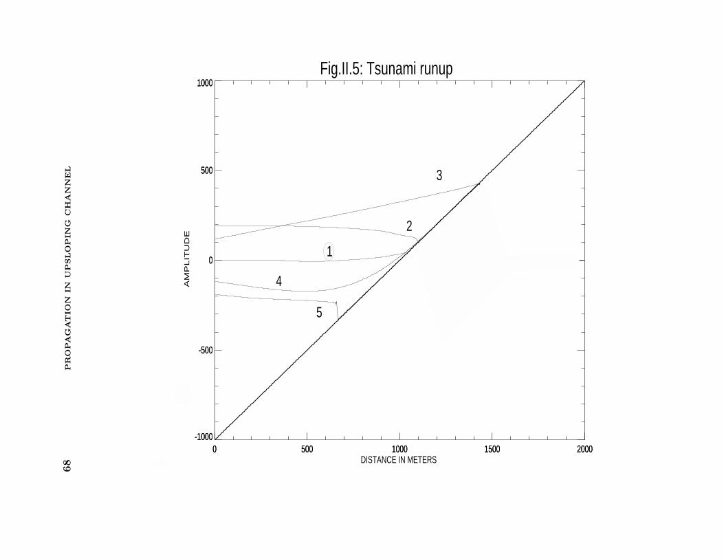
68P
RO
PA
GAT
ION
INU
PSLO
PIN
GC
HA
NN
EL
0 500 1000 1500 2000-1000
-500
0
500
1000
0 500 1000 1500 2000DISTANCE IN METERS
-1000
-500
0
500
1000
AM
PL
ITU
DE
1
1
2
3
4
5
Fig.II.5: Tsunami runup
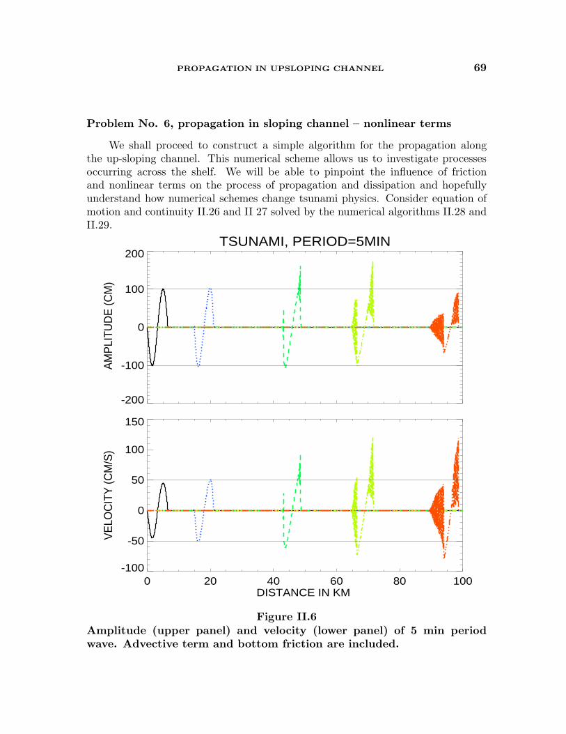
PROPAGATION IN UPSLOPING CHANNEL 69
Problem No. 6, propagation in sloping channel – nonlinear terms
We shall proceed to construct a simple algorithm for the propagation alongthe up-sloping channel. This numerical scheme allows us to investigate processesoccurring across the shelf. We will be able to pinpoint the influence of frictionand nonlinear terms on the process of propagation and dissipation and hopefullyunderstand how numerical schemes change tsunami physics. Consider equation ofmotion and continuity II.26 and II 27 solved by the numerical algorithms II.28 andII.29.
TSUNAMI, PERIOD=5MIN
-200
-100
0
100
200
AM
PLI
TUD
E (C
M)
0 20 40 60 80 100DISTANCE IN KM
-100
-50
0
50
100
150
VE
LOC
ITY
(CM
/S)
Figure II.6Amplitude (upper panel) and velocity (lower panel) of 5 min periodwave. Advective term and bottom friction are included.

70 PROPAGATION IN UPSLOPING CHANNEL
In this experiment the upsloping channel of 100 km length is considered. Depthis changing from 50 m at the entrance to 5 m at the end of the channel. We start bycomputing propagation of a 5 min period tsunami wave from the deep water towardsthe shallow water. Results are depicted in Fig.II.6. It is important to notice thelarge disparity in the sea level and velocity. While the sea level amplitude changesover a small range along the channel, velocity, on the other hand, displays muchgreater variations and is less prone to the dissipation. Here we investigate the wavebreaking process in the upsloping channel.
TSUNAMI, PERIOD=5MIN
-150
-100
-50
0
50
100
150
AM
PLI
TUD
E (C
M)
DX=25M, T=0.1 SEC; SECOND ORDER APPROXIMATION
0 20 40 60 80 100DISTANCE IN KM
-150
-100
-50
0
50
100
150
AM
PLI
TUD
E(C
M)
DX=5M, T=0.1 SEC; SECOND ORDER APPROXIMATION
Figure II.7
Wave traveling in upsloping channel. Solution obtained by eqs. (II.28)and (II.29). Upper panel: space step 25 m, lower panel: space step 5 m.

PROPAGATION IN UPSLOPING CHANNEL 71
Is this true physical process of the long wave breaking or this is a numericalartifact? The period is 600 s and the time step 0.1 s, thus the temporal resolution is6000SPP (step per period). The wavelength is changing from approximately 7 kmat the 50 m depth to 2 km at the 5 m depth. The latter is resolved with 25 m gridresulting in 80SPW, which is still an excellent resolution. Unfortunately, a sim-ple notion of the spatial and temporal resolution needs to be reexamined since inthe shallow water a strong nonlinear interaction occurs. This phenomenon shouldchange our approach to analyzing the numerical stability of the basic set of equa-tions, because previously we relied on the linear stability analysis only. Strongnonlinearities are often source of computational instabilities. To test whether theshort period waves, occuring at the head and tail of the main wave, are the part ofphysical phenomenon we carry out a simple experiment with an increased spatialresolution by taking step h=5m. The result of calculation is given in Fig. II.7. Inthe upper panel for comparison the result with h=25 m is also shown. The improve-ment in resolution (lower panel) leads to decreasing of the short wave oscillations.Therefore, we may conclude that the short wave oscillations is an computationalartifact caused by the poor space resolution.
The main source of nonlinear effects is the advective term. To the advectiveterm in eq. (II.26) the upwind method of the first order approximation in spaceis applied. For the stability reason we keep the upstream approach even with thehigher order of approximation for the first derivatives (see Kowalik and Bang, 1987).Construction of the first derivative can be carried out on the three-point or four-point stencil. For the three-point stencil the following construction can be used forthe advective term,
u∂u
∂x� up
(3umj − 4umj−1 + umj−2)2h
+ un(−umj+2 + 4umj+1 − 3umj )
2h+ O(h3) (II.31)
To bring the higher order of approximation to the entire set of equations to-gether with the advective term the higher order space derivatives for the sea leveland velocity in eqs. II.26 and II.27 has been used.
We start by constructing the space derivative for the sea level in the equation ofmotion II.26. The central point (u point) located in the j grid point is surrounded bythe two sea level grid points at the distance h/2 from the velocity point. Consideringtwo Taylor series for the sea level, one on the lattice h/2 and the second one onthe lattice 3h/2 by combining the two formulas the higher order formula can beconstructed. The new formula for the first derivative of the sea level in the u pointreads,
∂ζ
∂x= [27(ζj − ζj−1) − (ζj+1 − ζj−2)]/24h + O(h4) (II.32)
Space derivative for the velocity in the continuity equation II.27 is constructedin the similar way by noticing that the central point for such derivative is the sea
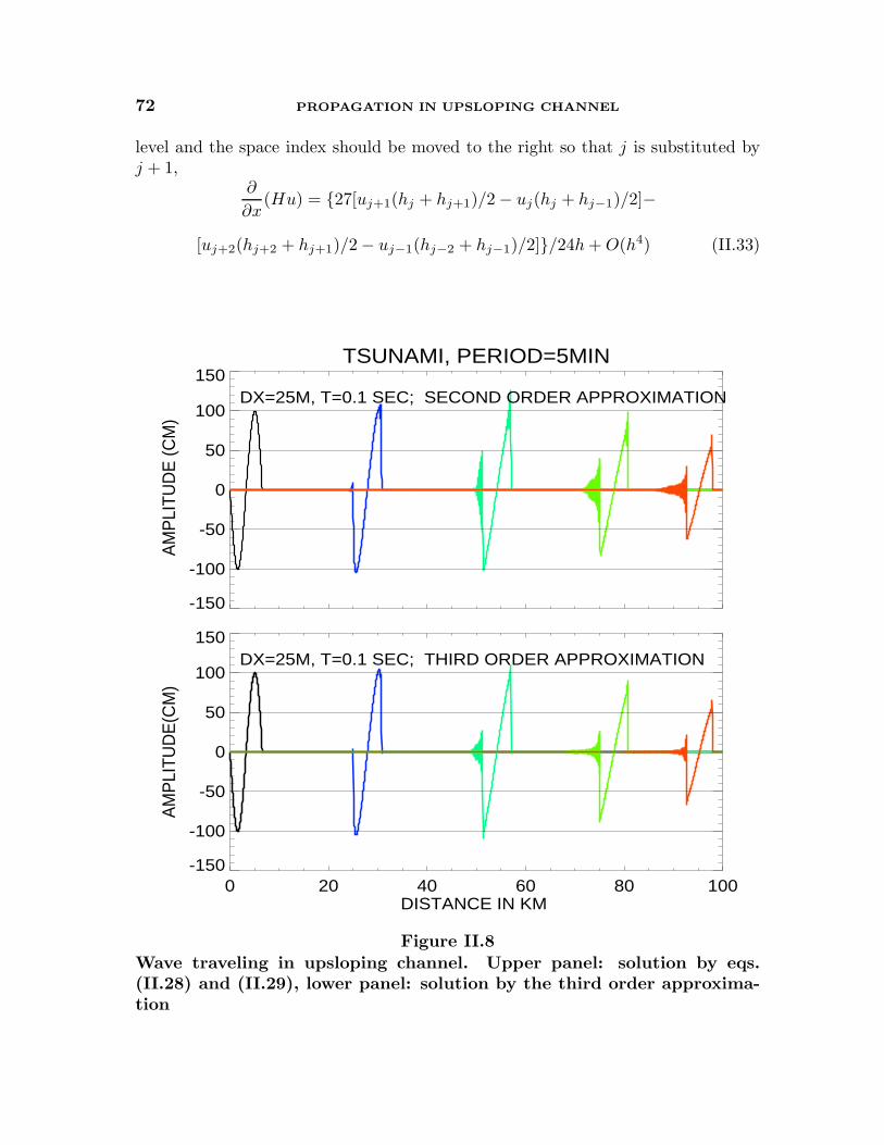
72 PROPAGATION IN UPSLOPING CHANNEL
level and the space index should be moved to the right so that j is substituted byj + 1,
∂
∂x(Hu) = {27[uj+1(hj + hj+1)/2 − uj(hj + hj−1)/2]−
[uj+2(hj+2 + hj+1)/2 − uj−1(hj−2 + hj−1)/2]}/24h + O(h4) (II.33)
TSUNAMI, PERIOD=5MIN
-150
-100
-50
0
50
100
150
AM
PLI
TUD
E (C
M)
DX=25M, T=0.1 SEC; SECOND ORDER APPROXIMATION
0 20 40 60 80 100DISTANCE IN KM
-150
-100
-50
0
50
100
150
AM
PLI
TUD
E(C
M)
DX=25M, T=0.1 SEC; THIRD ORDER APPROXIMATION
Figure II.8Wave traveling in upsloping channel. Upper panel: solution by eqs.(II.28) and (II.29), lower panel: solution by the third order approxima-tion

PROPAGATION IN UPSLOPING CHANNEL 73
Application of this approach to the advective term together with the higherorder derivatives (II.32) and (II.37) for the remaining space derivatives leads againto the improved results shown in the lower panel of Fig. II.8.
TSUNAMI, PERIOD=5MIN
-150
-100
-50
0
50
100
150
AM
PLI
TUD
E (C
M)
DX=25M, T=0.1 SEC; SECOND ORDER APPROXIMATION
0 20 40 60 80 100DISTANCE IN KM
-150
-100
-50
0
50
100
150
AM
PLI
TUD
E(C
M)
DX=25M, T=0.1 SEC; THIRD ORDER APPROXIMATION
AND FILTER
Figure II.9
Wave traveling in upsloping channel. Upper panel: solution by eqs.(II.28) and (II.29), lower panel: solution by the third order approxima-tion and space filter
Conclusion from the above experiments is that the parasitic short wave os-cillations can be deleted through an application of the high spatial and temporalresolutions. A somewhat different and easier solution is application of a simple

74 PROPAGATION IN UPSLOPING CHANNEL
space filter. It is applied only to the computed velocity. The new velocity um+1j is
filtered in the following manner,
UN(J) = um+1j ∗ (1 − ALP ) + 0.25 ∗ (um+1
j−1 + 2. ∗ um+1j + um+1
j+1 ) ∗ALP (II.34)
The filter parameter ALP = 0.005. The computation carried out with the highorder derivatives and the above filter are shown in the lower panel of Fig. II.9
Program to perform above calculations is constructed in very similar way asthe previous programs. Here the variable depth from 50m to 5m is considered.
!Program upslopeProgram channel! PROGRAM COMPUTE propagation in 1D upward sloping channel! by the higher order methods! program originated by Z.K. at IMS, AlaskaINTEGER,PARAMETER:: je=4001,JS=1,MON= 65001INTEGER::NS,MON1REAL,DIMENSION(1:JE)::U,UN,Z,ZN,
H,H1,DU,U2N,U2P,AN,UF,UN1,UN2REAL,PARAMETER::HL=5000.,HR=500.,ADV=1.,B=1.,R=0.0033! REAL,PARAMETER::HL=5000.,HR=500.,ADV=.0,B=0.,R=0.0open (unit=10,file=’amp5.dat’,status=’unknown’)open (unit=12,file=’vel3.dat’,status=’unknown’)OPEN(UNIT=11,FILE=’depth.dat’,STATUS=’unknown’)! MON is total number of time steps! if B=1 total depth is computed H1=H+Z*B! IF ADV=1, NONLINEAR TERMS ARE IN! R BOTTOfM FRICTION COEFFICIENTMON1=MON/200G=982.TM2=44714.1353 ! M2 TIDE PERIODTP=300.PI=3.141592653589793238462643383279502884197! time step and space stept=0.1 !0.1SDX=2500. ! 25 meters!NUMBER OF TIME STEPS IN TSUNAMI PERIODns=INT(TP/T)! PRINT *,NS! COEFFICIENTS FOR EQUATIONSPL=2.0*T/DXPLG=G*PL! depth from HL= 50M AT J=1 to HR= 5M AT J=JE
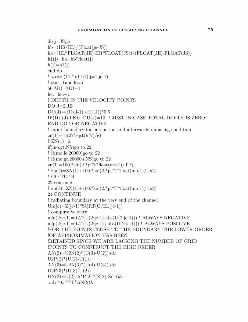
PROPAGATION IN UPSLOPING CHANNEL 75
do j=JS,jehb=(HR-HL)/(Float(je-JS))ha=(HL*FLOAT(JE)-HR*FLOAT(JS))/(FLOAT(JE)-FLOAT(JS))h1(j)=ha+hb*float(j)h(j)=h1(j)end do! write (11,*)(h1(j),j=1,je-1)! start time loop50 MO=MO+1leu=leu+1! DEPTH IN THE VELOCITY POINTSDO J=2,JEDU(J)=(H1(J-1)+H1(J))*0.5IF(DU(J).LE.0.)DU(J)=10. ! JUST IN CASE TOTAL DEPTH IS ZEROEND DO ! OR NEGATIVE! input boundary for one period and afterwards radiating conditionzn(1)=-u(2)*sqrt(h(2)/g)! ZN(1)=0.if(mo.gt.NS)go to 22! if(mo.le.20000)go to 22! if(mo.gt.20000+NS)go to 22zn(1)=100.*sin(2.*pi*t*float(mo-1)/TP)! zn(1)=ZN(1)+100.*sin(2.*pi*T*float(mo-1)/tm2)! GO TO 2422 continue! zn(1)=ZN(1)+100.*sin(2.*pi*T*float(mo-1)/tm2)24 CONTINUE! radiating boundary at the very end of the channelUn(je)=Z(je-1)*SQRT(G/H1(je-1))! compute velocityu2n(2:je-1)=0.5*(U(2:je-1)-abs(U(2:je-1))) ! ALWAYS NEGATIVEu2p(2:je-1)=0.5*(U(2:je-1)+abs(U(2:je-1))) ! ALWAYS POSITIVE!FOR THE POINTS CLOSE TO THE BOUNDARY THE LOWER ORDER!OF APPROXIMATION HAS BEEN!RETAINED SINCE WE ARE LACKING THE NUMBER OF GRID!POINTS TO CONSTRUCT THE HIGH ORDERAN(2)=U2N(2)*(U(3)-U(2))+&U2P(2)*(U(2)-U(1))AN(3)=U2N(3)*(U(4)-U(3))+&U2P(3)*(U(3)-U(2))UN(2)=U(2)-.5*PLG*(Z(2)-Z(1))&-adv*0.5*PL*AN(2)&

76 PROPAGATION IN UPSLOPING CHANNEL
-r*T*U(2)*abs(U(2))/DU(2)UN2(2)=UN(2)UN1(2)=UN(2)AN(JE-1)=U2N(JE-1)*(U(JE)-U(JE-1))+&U2P(JE-1)*(U(JE-1)-U(JE-2))AN(JE-2)=U2N(JE-2)*(U(JE-1)-U(JE-2))+&U2P(JE-2)*(U(JE-2)-U(JE-3))! HIGHER ORDER FOR ADVECTIVE TERMAN(3:JE-2)= U2N(3:JE-2)*(-U(5:JE)+4.*U(4:JE-1)-3.*U(3:JE-2))/2.+ &U2P(3:JE-2)*(3.*U(3:JE-2)-4.*U(2:JE-3)+U(1:JE-4))/2. !THIRD DERIVA-
TIVE! AN(3:JE-2)=U2N(3:JE-2)*(-U(5:JE)+6.*U(4:JE-1)-!3.*U(3:JE-2)-2.*U(2:JE-3))/6.+&! U2P(3:JE-2)*(2.*U(4:JE-1)+3.*U(3:JE-2)!-6.*U(2:JE-3)+U(1:JE-4))/6. ! fOURTH DERIVATIVE! AN(4:JE-3)= U2N(4:JE-3)*(2.*U(7:JE)-9.*U(6:JE-1)!+18*U(5:JE-2)-11.*U(4:JE-3))/6.+&! U2P(4:JE-3)*(-2.*U(1:JE-6)+9.*U(2:JE-5)!-18*U(3:JE-4)+11.*U(4:JE-3))/6.DO 80 J=3,je-2!LOWER ORDER APPROXIMATION!UN(J)=U(J)-.5*PLG*(Z(J)-Z(J-1)) &!-adv*0.5*PL*(u2p(J)*(U(j)-U(j-1))+u2n(J)*(U(j+1)-U(j)))&!-r*T*U(j)*abs(U(j))/DU(J)! HIGHER ORDER OF APPROXIMATIONA1=27.*(Z(J)-Z(J-1))A2=Z(J+1)-Z(J-2)UN(J)=U(J)-.5*PLG*(A1-A2)/24.&-adv*0.5*PL*AN(J)&-r*T*U(j)*abs(U(j))/DU(J)80 CONTINUE! USE FILTER - FOR THIS PURPOSE CHANGE IN THE ABOVE!FORMULA UN TO UN1 SO THAT UN COMES OUT OF FILTER! DO J=3,JE-2! UN2(J)=UN1(J)-adv*0.5*PL*AN(J)! END DO! DO J=3,JE-2! ALP=0.005! UN(J)= UN1(J)*(1-ALP)+0.25*(UN1(J-1)+2.*UN1(J)+UN1(J+1))*ALP! END DO! compute sea levelDO 120 J=2,je-1
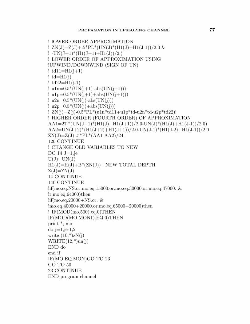
PROPAGATION IN UPSLOPING CHANNEL 77
! lOWER ORDER APPROXIMATION! ZN(J)=Z(J)+.5*PL*(UN(J)*(H1(J)+H1(J-1))/2.0 &! -UN(J+1)*(H1(J+1)+H1(J))/2.)! LOWER ORDER OF APPROXIMATION USING!UPWIND/DOWNWIND (SIGN OF UN)! td11=H1(j+1)! td=H1(j)! td22=H1(j-1)! u1n=0.5*(UN(j+1)-abs(UN(j+1)))! u1p=0.5*(UN(j+1)+abs(UN(j+1)))! u2n=0.5*(UN(j)-abs(UN(j)))! u2p=0.5*(UN(j)+abs(UN(j)))! ZN(j)=Z(j)-0.5*PL*(u1n*td11+u1p*td-u2n*td-u2p*td22)!! HIGHER ORDER (FOURTH ORDER) OF APPROXIMATIONAA1=27.*(UN(J+1)*(H1(J)+H1(J+1))/2.0-UN(J)*(H1(J)+H1(J-1))/2.0)AA2=UN(J+2)*(H1(J+2)+H1(J+1))/2.0-UN(J-1)*(H1(J-2)+H1(J-1))/2.0ZN(J)=Z(J)-.5*PL*(AA1-AA2)/24.120 CONTINUE! CHANGE OLD VARIABLES TO NEWDO 14 J=1,jeU(J)=UN(J)H1(J)=H(J)+B*(ZN(J)) ! NEW TOTAL DEPTHZ(J)=ZN(J)14 CONTINUE140 CONTINUE!if(mo.eq.NS.or.mo.eq.15000.or.mo.eq.30000.or.mo.eq.47000. &!r.mo.eq.64000)then!if(mo.eq.20000+NS.or. &!mo.eq.40000+20000.or.mo.eq.65000+20000)then! IF(MOD(mo,500).eq.0)THENIF(MOD(MO,MON1).EQ.0)THENprint *, modo j=1,je-1,2write (10,*)zN(j)WRITE(12,*)un(j)END doend ifIF(MO.EQ.MON)GO TO 23GO TO 5023 CONTINUEEND program channel

78 RECTANGULAR AND NON-RECTANGULAR WATER BODIES
3. Rectangular and non-rectangular water bodies
Here the vertically integrated equations will be rendered into numerical form forthe rectangular water bodies. This problem is well described in Ch.III, Sec.4 of NM.In the brief explanation given below we shall use equations in both rectangular andspherical coordinate systems. Rectangular system is used because it is simple in theapplications, but when the horizontal scale of a computational domain is exceeding1000km the spherical system must be used to describe properly all consequencesrelated to the spherical shape of Earth. For numerical formulation in rectangularsystem we shall use eqs. (3.95)-(3.97) from NM with modifications made in thefrictional terms. These terms instead at time m − 1, as in NM, will be taken attime step m.
um+1j,k − umj,k
T+ UPOS(umj,k − umj−1,k)/h + UNEG(umj+1,k − umj,k)/h
+V AUP (umj,k − umj,k−1)/h + V AUN(umj,k+1 − umj,k)/h
−f vu,m = − g
h(ζmj,k − ζmj−1,k) +
1ρoDm
u,j,k
(τ s,mx,j,k
−Rmx,j,ku
mj,k) +
Nh
h2(umj+1,k + umj−1,k + umj,k+1 + umj,k−1 − 4umj,k) (II.35)
vm+1j,k − vmj,k
T+ UAV P (vmj,k − vmj−1,k)/h + UAV N(vmj+1,k − vmj,k)/h
+V POS(vmj,k − vmj,k−1)/h + V NEG(vmj,k+1 − vmj, k)/h
+fuv,m+1 = − g
h(ζmj,k+1 − ζmj,k) +
1ρoDm
v,j,k
(τ s,my,j,k
−Rmy,j,kv
mj,k) +
Nh
h2(vmj+1,k + vmj−1,k + vmj,k+1 + vmj,k−1 − 4vmj,k) (II.36)
ζm+1j,k − ζmj,k
T= − 1
h(um+1
j+1,kDmu,j+1,k − um+1
j,k Dmu,j,k)− 1
h(vm+1
j,k Dmv,j,k − vm+1
j,k−1Dmv,j,k−1)
(II.37)The nonlinear terms are given according to the upwind–downwind approximationintroduced in Ch.II of NM. The following notation is used:
UPOS = (umj,k + |umj,k|)/2 UNEG = (umj,k − |umj,k|)/2
V AUP = (vu,m + |vu,m|)/2 V AUN = (vu,m − |vu,m|)/2
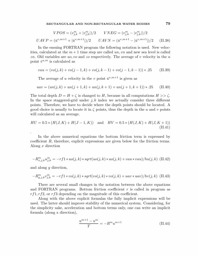
RECTANGULAR AND NON-RECTANGULAR WATER BODIES 79
V POS = (vmj,k + |vmj,k|)/2 V NEG = (vmj,k − |vmj,k|)/2
UAV P = (uv,m+1 + |uv,m+1|)/2 UAV N = (uv,m+1 − |uv,m+1|)/2 (II.38)
In the ensuing FORTRAN program the following notation is used. New veloc-ities, calculated at the m + 1 time step are called un, vn and new sea level is calledzn. Old variables are uo, vo and zo respectively. The average of v velocity in the upoint vu,m is calculated as
vau = (vo(j, k) + vo(j − 1, k) + vo(j, k − 1) + vo(j − 1, k − 1)) ∗ .25 (II.39)
The average of u velocity in the v point uv,m+1 is given as
uav = (un(j, k) + un(j + 1, k) + un(j, k + 1) + un(j + 1, k + 1)) ∗ .25 (II.40)
The total depth D = H + ζ is changed to H, because in all computations H >> ζ.In the space staggered-grid under j, k index we actually consider three differentpoints. Therefore, we have to decide where the depth points should be located. Agood choice is usually to locate it in ζ points, thus the depth in the u and v pointswill calculated as an average.
HU = 0.5 ∗ (H(J,K) + H(J − 1, K)) and HV = 0.5 ∗ (H(J,K) + H(J,K + 1))(II.41)
.In the above numerical equations the bottom friction term is expressed by
coefficient R, therefore, explicit expressions are given below for the friction terms.Along x direction
−Rmx,j,ku
mj,k = −rf1 ∗uo(j, k) ∗ sqrt(uo(j, k) ∗uo(j, k) + vau ∗ vau)/hu(j, k) (II.42)
and along y direction,
−Rmy,j,kv
mj,k = −rf1 ∗ vo(j, k) ∗ sqrt(vo(j, k) ∗ vo(j, k) + uav ∗ uav)/hv(j, k) (II.43)
There are several small changes in the notation between the above equationsand FORTRAN programs. Bottom friction coefficient r is called in program asrf1, rf2, or rf3 depending on the magnitude of this coefficient.
Along with the above explicit formulas the fully implicit expressions will beused. The latter should improve stability of the numerical system. Considering, forthe simplicity sake, acceleration and bottom terms only, one can write an implicitformula (along x direction),
um+1 − um
T= −Rmum+1 (II.44)
80 RECTANGULAR AND NON-RECTANGULAR WATER BODIES
To calculate velocity at the m + 1 time step from (II.44) one obtains,
um+1 =um
(1 + TRm)(II.45)
Horizontal friction in all equations is denoted as Nh but in the FORTRANprogram is called ah. To improve stability, along with the explicit algorithm we shalluse semi-implicit formulas given by (3.94a) from NM. Considering only horizontalfriction and acceleration
um+1j − umj
T=
Nh
h2[(umj+1 − umj ) − (um+1
j − um+1j−1 )] (II.46)
The new velocity will be computed as
um+1j = umj
h2
h2 + TNh+ coef(umj+1 + um+1
j−1 − umj ) (II.47)
Herecoef =
TNh
(h2 + TNh)
We have also introduced coefficients called cfric, cnl2, and ccor, equal to 0 or 1,with the aim of facilitating numerical experiments by switching off and on variousterms in the equations. Coriolis parameter f is equal 2w sinφ.
In the spherical system of coordinate we shall use the vertically integratedequation of motion and continuity (1.92)–(1.95) from Ch.I of NM.
Du
Dt− fv − uv sinφ
R cosφ= − g
R cosφ∂ζ
∂λ+
τ sλ − τ bλρD
+ Au (II.48)
Dv
Dt+ fu +
uu sinφ
R cosφ= − g
R
∂ζ
∂φ+
τ sφ − τ bφρD
+ Av (II.49)
∂ζ
∂t+
1R cosφ
∂(Du)∂λ
+1
R cosφ∂
∂φ(Dv cosφ) = 0 (II.50)
Here
D
Dt=
∂
∂t+
u
R cosφ∂
∂λ+
v
R
∂
∂φ(II.51)
The advective nonlinear terms in (II.51) are about two orders of magnitudelarger than the remaining nonlinear terms in (II.48) and (II.49), therefore in ensuingcomputations only advective nonlinear terms are taken into account.
The operator in the horizontal friction term in (II.48) and (II.49) is
RECTANGULAR AND NON-RECTANGULAR WATER BODIES 81
A = Nh(1
R2 cos2 φ∂2
∂λ2+
1R2 cosφ
∂
∂φ(cosφ
∂
∂φ)) (II.52)
The bottom friction components are taken as
τ bλ = ρru√
u2 + v2; τ bφ = ρrv√
u2 + v2. (II.53)
Numerical form of the equations written in the spherical coordinates differsonly slightly from equations given above for the rectangular system.
To control the computation one can check temporal and spatial behavior ofthe sea level and velocities. Therefore the sea level is recorded in a few grid-pointsand time series are plotted. We assume that the time change of the sea level willshed some light on the temporal behavior of the computed process. For exampletime series for the tides should behave in the oscillatory manner. Time series forthe motion imparted by the constant wind should arrive to the steady state aftertransient processes will decay.
The total energy of the system, i.e. kinetic and potential energy calculatedover the entire domain is also a very good parameter for checking the behavior ofthe system and especially its temporal properties. Total energy in the FORTRANprogram is called eni and is calculated in the sea level point. Velocities required forthe calculations are taken as average from the neighboring points. Formula (3.5a)from NM is used for the calculations.
Problem No. 7, storm surge in rectangular domain
To learn about intricate problems of the 2-D modeling we shall consider arectangular water body 1500km by 1500km, with gently sloping bottom from 200mto 20m along x direction. Along y direction depth is constant. Along x directionwind is blowing, changing linearly in time from 0 to 2 CGS in two hours, andremains constant thereafter. The time step of numerical integration is 100s, andspace step is 10 km. Below, the FORTRAN program surge.f is given.
c=========================================C PROGRAM SURGE.FC ORIGINATED BY Z.K. AT IMSc program to compute storm surge in the rectangular domainsparameter (jx=150,ky=150)dimension uo(jx,ky),un(jx,ky),vo(jx,ky),vn(jx,ky),* zo(jx,ky),zn(jx,ky)c uo, un, vo, vn old and new velocity component along x (longitude)c and along y (latitude)c zo and zn old and new sea leveldimension h(jx,ky),hu(jx,ky),hv(jx,ky),eni(500)

82 RECTANGULAR AND NON-RECTANGULAR WATER BODIES
c depth h and depth dependent functions hu,hv (averages along x and y direc-tions)
c eni is total energy of the systemcdimension cfric(jx,ky),ccor(jx,ky),cnl2(jx,ky)c cfric,ccor,cnl2 coefficients equal to 1 or 0 to switch off and onc friction, coriolis and nonlinear termsdimension taux(jx,ky),tauy(jx,ky)c wind stress along x and yopen (unit=10,file=’zn.dat’,status=’unknown’) ! sea levelopen (unit=20,file=’momaxm2.dat’,status=’unknown’) ! time seriesopen (unit=21,file=’un.dat’,status=’unknown’) ! u-velocityopen (unit=22,file=’vn.dat’,status=’unknown’) ! v-velocityopen (unit=25,file=’enim2.dat’,status=’unknown’) ! energypi = 4.*atan(1.)rad = pi/180.c grid size along x (longitude) and y (latitude)dx=1.0e6 ! 10km grid step expressed in cmdy=1.0e6 ! dx and dy may be differentblat = 50 ! lat 50 degree, it stays constant in domainblatr=50*pi/180.c set depth distribution (from 200m to 20m in x direction,c or constant equal to 200m)do j=1,jxdo k=1,kyh(j,k)=(201.20805-1.20805*float(j))*1.0e2c h(j,k)=20000. ! constant depthenddoenddoprint *, h(30,30)cc Intialize constantscw=7.29e-05 !angular velocity of earthrf1=3.3e-03 !coefficient of friction (in cgs) - open oceanrf2=6.6e-03 !coefficient of friction (in cgs) - shelfrf3=1.e-02 !coefficient of friction (in cgs) - shallow waterrf4=3.e-02 !coefficient of friction (in cgs) - on landcc controlling coefficients : cfric = bottom friction termc ccor = coriolis termc cnl2 = non-linear term
RECTANGULAR AND NON-RECTANGULAR WATER BODIES 83
do j=1,jxdo k=1,kycfric(j,k) = 1.ccor(j,k) = 1.cnl2(j,k) = 1.end doend doc t : time step in secondct = 100.c maximum time stepsmomax=10000g=981.c ah=0. ! horizontal eddy viscosityah=5.0e9 ! unstable in explicit schemec ah = 5.0e7c ah = 2.0e7c coefficients for the equationsc combination of space steps and time stepspl = t/(dx)pf = t/(dy)pr1 = t*rf1pr2 = t*rf2pr3 = t*rf3pr4 = t*rf4pw = t*2*wptc=pw*sin(blatr)ph1 = ah*t/(dx*dx)ph2 = ah*t/(dy*dy)gpl=g*plgpf=g*pfc this variables are related to depth distributions andc are used mainly in equation of continuitydo j=2,jxdo k=1,kyhu(j,k)=0.5*(h(j,k)+h(j-1,k)) ! depth in the U pointsend doend dodo j=1,jxdo k=1,ky-1hv(j,k) = (h(j,k)+h(j,k+1))*.5 ! depth in the V pointsend do
84 RECTANGULAR AND NON-RECTANGULAR WATER BODIES
end doc **************************************************************c * main computation loop *c * u : horizontal particle velocity in east/west direction *c * v : horizontal particle velocity in north/south direction *c * z : sea level variation in cm *c **************************************************************c===========================================do 3000 mo= 1,momaxc specify wind driven forces, first seventy two time steps linear grow in timec of taux from 0 to 2.01 tauy=0. Aand afterwards taux=2.01motau=72r=mo/motauif(r.gt.1)r=1.do j=1,jxdo k=1,kytaux(j,k)= 2.01*rtauy(j,k)=0.end doend doc
*******************************************************************c U-Computationc domaindo j=2,jx-1do k=2,ky-1vau = (vo(j,k)+vo(j-1,k)+vo(j,k-1)+vo(j-1,k-1))*.25upos = .5*(uo(j,k)+abs(uo(j,k)))uneg = .5*(uo(j,k)-abs(uo(j,k)))vaup = .5*(vau+abs(vau))vaun = .5*(vau-abs(vau))uojk=uo(j,k)un(j,k) = uojk+T*taux(j,k)/hu(j,k)& - gpl*(zo(j,k)-zo(j-1,k))& + ptc*vau*ccor(j,k)c & +ph1*(uo(j+1,k)+uo(j-1,k)-2.*uojk) ! explicit hor. frictionc & +ph2*(uo(j,k+1)+uo(j,k-1)-2.*uojk) ! explicit hor. frictionc & -pr1*uojk*sqrt(uojk*uojk+vau*vau)/hu(j,k)*cfric(j,k) !expl.bottomc if explicit method is used uncomment 3 above lines and delete allc lines below down to endo& +ph1*(uo(j+1,k)+un(j-1,k)-uojk) ! semi-expl&+ph2*(uo(j,k+1)+un(j,k-1)-uojk) ! semi-expl

RECTANGULAR AND NON-RECTANGULAR WATER BODIES 85
&-pl*(upos*(uo(j,k)-uo(j-1,k))+uneg*(uo(j+1,k)-uo(j,k)))*cnl2(j,k)&-pf*(vaup*(uo(j,k)-uo(j,k-1))+vaun*(uo(j,k+1)-uo(j,k)))*cnl2(j,k)hfr2=ph1+ph2uni=1.+hfr2+pr1*sqrt(uojk*uojk+vau*vau)/hu(j,k)*cfric(j,k)un(j,k)=un(j,k)/unienddoenddoc
*******************************************************************cc V-Computationdo j=2,jx-1do k=2,ky-2uav = (un(j,k)+un(j+1,k)+un(j,k+1)+un(j+1,k+1))*.25uavp = .5*(uav+abs(uav))uavn = .5*(uav-abs(uav))vpos = .5*(vo(j,k)+abs(vo(j,k)))vneg = .5*(vo(j,k)-abs(vo(j,k)))vojk=vo(j,k)vn(j,k) = vojk+T*tauy(j,k)/hv(j,k)& - gpf*(zo(j,k+1)-zo(j,k))& - ptc*uav*ccor(j,k)c & +ph1*(vo(j+1,k)+vo(j-1,k)-2.*vojk)c & +ph2*(vo(j,k+1)+vo(j,k-1)-2.*vojk)c & -pr1*vojk*sqrt(vojk*vojk+uav*uav)/hv(j,k)*cfric(j,k)& +ph1*(vo(j+1,k)+vn(j-1,k)-vojk) ! semi-explicit&+ph2*(vo(j,k+1)+vn(j,k-1)-vojk) ! semi-explicit&-pf*(vpos*(vo(j,k)-vo(j,k-1))+vneg*(vo(j,k+1)-vo(j,k)))*cnl2(j,k)&-pl*(uavp*(vo(j,k)-vo(j-1,k))+uavn*(vo(j+1,k)-vo(j,k)))*cnl2(j,k)hfr1=ph1+ph2vni=1.+hfr1+pr1*sqrt(vojk*vojk+uav*uav)/hv(j,k)*cfric(j,k)vn(j,k)=vn(j,k)/vnienddoenddoc
*******************************************************************cc Z - computationdo j=1,jx-1do k=2,ky-1zn(j,k)=zo(j,k)-pl*(un(j+1,k)*hu(j+1,k)-un(j,k)*hu(j,k))* - hv(j,k)*vn(j,k)*pf+pf*vn(j,k-1)*hv(j,k-1)
86 RECTANGULAR AND NON-RECTANGULAR WATER BODIES
enddoenddoc **************************************************************cc update old variables with newdo j=1,jxdo k=1,kyuo(j,k)=un(j,k)vo(j,k)=vn(j,k)zo(j,k)=zn(j,k)enddoenddoc ****************************************************************ccif(mod(mo,20).eq.0) thenc Computing kinetic and potential energy every 20 stepsc ENI enrgy every 20 steps , averaged over whole spaceNC=MO/20ES=0.do j=1,jx-1do k=2,kyua=0.5*(un(j,k)+un(j+1,k))va=0.5*(vn(j,k)+vn(j,k-1))en=h(j,k)*(ua*ua+va*va)/(2.*g)+zn(j,k)*zn(j,k)/2.es=en+esend doend doeni(nc)=eswrite(25,*)esendifif(mod(mo,20).eq.0) thenprint *, ’MO=’,mo, ’entrance=’,zn(2,10)print *, ’east basin=’,zn(50,10)print *,’west basin=’,zn(125,10)write(20,*),mo,zn(2,10),zn(50,10),zn(145,10)endifif(mod(mo,8640).eq.0) thenc sea level and velocity in whole domain at day 10write(10,*)((zn(j,k),j=1,jx),k=1,ky)write(21,*)((un(j,k),j=1,jx),k=1,ky)write(22,*)((vn(j,k),j=1,jx),k=1,ky)

RECTANGULAR AND NON-RECTANGULAR WATER BODIES 87
endif3000 continuestopendc===================================
This simple program open numerous possibilities to study process of stormsurge generation and propagations under various conditions. Before embarking thistrain one should carefully study numerical properties of the algorithm used. Somecoefficients in the numerical system are either variable or not well established. Tosuch category belongs horizontal eddy viscosity coefficient. A few experiments withan explicit numerical formulation for the horizontal eddy viscosity will demonstratethat this numerical scheme is both unstable for the large and small eddy viscositycoefficients. Does window for the numerical stability cover the whole range of nec-essary variation from the physical point of view? Surely not, and therefore, we haveintroduced a semi-explicit scheme with stronger stability properties. A few resultsare given in Figs. II.10 and II.11. In Fig.II.10 the sea level distribution in the wholedomain is depicted at day 10 of the process. As one should expect along a shalloweastern shoreline the sea level is high and at the western shoreline the sea level isnegative. It is always important to ask whether this result is correct. In the case ofthe sea level any forcing involved in the closed domain should retain an average sealevel equal to zero. Therefore, to test this assumption the results of computationsfor the sea level should be summed up over all grid points.
In Fig.II.11 we depicted total energy of the system. Due to steady wind one canexpect that the energy of the system will arrive to constant value as well. It does,but quite slowly, depicting some decaying oscillations. We have done computationswith the two horizontal eddy viscosity coefficients and clearly the large coefficientdamps oscillations much faster. Temporal behavior of the energy is motivatingfurther important questions. First, we may ask: what are these oscillations? Afterelucidating the nature of the oscillations, we may ask more important question:can we use this approach to study these oscillations? So, at this juncture we area bit away from our main topic i.e., study of the storm surges, but serendipity innumerical computations happens through the skillful invoking of the side questions.
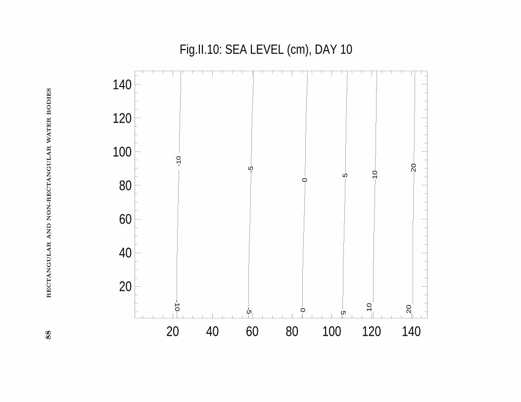
88R
EC
TA
NG
ULA
RA
ND
NO
N-R
EC
TA
NG
ULA
RW
AT
ER
BO
DIE
SFig.II.10: SEA LEVEL (cm), DAY 10
20 40 60 80 100 120 140
20
40
60
80
100
120
140
5
5
10
10
-10
-10
-5
-5
0
0
20
20-1
0
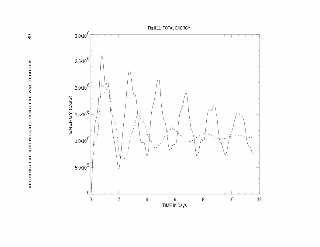
REC
TA
NG
ULA
RA
ND
NO
N-R
EC
TA
NG
ULA
RW
AT
ER
BO
DIE
S89
Fig.II.11: TOTAL ENERGY
0 2 4 6 8 10 12TIME in Days
0
5.0•10 5
1.0•10 6
1.5•10 6
2.0•10 6
2.5•10 6
3.0•10 6
EN
ER
GY
(C
GS
)
90 RECTANGULAR AND NON-RECTANGULAR WATER BODIES
Problem No. 8, storm surge in the non-rectangular domain
To calculate storm surges in the non-rectangular domains we need to learnhow to account for the complicated shape of the domain. In irregular water bodieswe first learn how to enumerate the grid points which are located in water. Anexplanation of such procedure is given on p. 134 of NM. We shall explore first thisprocedure to establish the set of indices for the horizontal u velocity computation.Thus checking each row from k=1 to k=ky, one can locate in every row the startingpoint (js) and the ending point (je) of the water domain along the x axis. The depthover the land and along the coastal lines is set to zero. Because of islands it mayhappen that in the some row (same k) a few different starting and ending points willbe prescribed. This is done in the program by counting the number of segments.An individual segment in the program is called, a line. Proceeding in similar wayfrom the first column (j=1) to the last column (j=jx), one can establish beginningand ending indices for the v velocity integration along the y direction. This is alldone in the FORTRAN program named index.f (see Chap.3 of this Workbook). Theprogram reads depth distribution from the file parab.dat (again, see Chap.3) andoutputs indices for the u, v and sea level integration. It also calculates the numberof lines along the x and y direction, therefore every set of indices can be related tothe proper line number.
The program to compute storm surges is called surge1.f and is listed below.The main difference between surge.f and surge1.f occurs in the space integration.Velocity along x direction is computed in the loop 4. First this loop counts linenumber. This number proceeds from 1 to nlh, which is the total number of rows(horizontal lines). Beginning of every line is given by js(n)+1, and the end is setby je(n). We keep also the index of an row (k index). Horizontal lines also serveto calculate the new sea level (loop 13). Here index j starts from js(n), i.e., thenumber of the sea level points is equal to the number of u velocity points plus one.Calculation of the v velocity is proceeding along the vertical lines (columns). Totalnumber of columns is equal to nlv.
C PROGRAM SURGE1.FC ORIGINATED BY Z.K. AT IMSc program to compute storm surge in the 2-d domains of any shapeparameter (jx=21,ky=21,nlh=17,nlv=17)dimension uo(jx,ky),un(jx,ky),vo(jx,ky),vn(jx,ky),* zo(jx,ky),zn(jx,ky)c uo, un, vo, vn old and new velocity component along x (longitude)c and along y (latitude)c zo and zn old and new sea leveldimension h(jx,ky),hu(jx,ky),hv(jx,ky),eni(500)c depth h and depth dependent functions hu,hv (averages along x and y direc-
tions)
RECTANGULAR AND NON-RECTANGULAR WATER BODIES 91
c eni is total energy of the systemcdimension cfric(jx,ky),ccor(jx,ky),cnl2(jx,ky)c cfric,ccor,cnl2 coefficients equal to 1 or 0 to switch off and onc friction, coriolis and nonlinear termsdimension taux(jx,ky),tauy(jx,ky)c wind stress along x and yinteger js(nlh),je(nlh),ks(nlh),ke(nlh)c indices along x directioninteger jsv(nlv),jev(nlv),ksv(nlv),kev(nlv)c indices along y directionopen (unit=4,file=’parab.dat’,status=’unknown’)c depth fileopen (unit=3,file=’parab.ind’,status=’unknown’)c file to keep indicesc read depthread(4,*)((h(j,k),j=1,JX),k=1,ky)c Index : horizontal lines and vertical linesdo i=1,nlhread (3,100) ks(i),ke(i),js(i),je(i)100 format(4i4)enddodo i=1,nlvread (3,100) jsv(i),jev(i),ksv(i),kev(i)enddocclose (3)open (unit=10,file=’zn.dat’,status=’unknown’) ! sea levelopen (unit=20,file=’momaxm2.dat’,status=’unknown’) ! time seriesopen (unit=21,file=’un.dat’,status=’unknown’) ! u-velocityopen (unit=22,file=’vn.dat’,status=’unknown’) ! v-velocityopen (unit=25,file=’enim2.dat’,status=’unknown’) ! energypi = 4.*atan(1.)rad = pi/180.c grid size along x (longitude) and y (latitude)dx=1.0e6 ! 10km grid step expressed in cmdy=1.0e6 ! dx and dy may be differentblat = 50 ! lat 50 degree, it stays constant in domainblatr=50*pi/180.print *, h(8,8)cc Intialize constants
92 RECTANGULAR AND NON-RECTANGULAR WATER BODIES
cw=7.29e-05 !angular velocity of earthrf1=3.3e-03 !coefficient of friction (in cgs) - open oceanrf2=6.6e-03 !coefficient of friction (in cgs) - shelfrf3=1.e-02 !coefficient of friction (in cgs) - shallow waterrf4=3.e-02 !coefficient of friction (in cgs) - on landcc controlling coefficients : cfric = bottom friction termc ccor = coriolis termc cnl2 = non-linear termdo j=1,jxdo k=1,kycfric(j,k) = 1.ccor(j,k) = 1.cnl2(j,k) = 1.end doend doc t : time step in secondct = 100.c maximum time stepsmomax=10000g=981.c ah=0. ! horizontal eddy viscosityc ah=5.0e9 ! unstable in explicit schemec ah = 5.0e7ah = 2.0e7c coefficients for the equationsc combination of space steps and time stepspl = t/(dx)pf = t/(dy)pr1 = t*rf1pr2 = t*rf2pr3 = t*rf3pr4 = t*rf4pw = t*2*wptc=pw*sin(blatr)ph1 = ah*t/(dx*dx)ph2 = ah*t/(dy*dy)gpl=g*plgpf=g*pfc this variables are related to depth distributions and

RECTANGULAR AND NON-RECTANGULAR WATER BODIES 93
c are used mainly in equation of continuitydo j=2,jxdo k=1,kyhu(j,k)=0.5*(h(j,k)+h(j-1,k)) ! depth in the U pointsend doend dodo j=1,jxdo k=1,ky-1hv(j,k) = (h(j,k)+h(j,k+1))*.5 ! depth in the V pointsend doend doc **************************************************************c * main computation loop *c * u : horizontal particle velocity in east/west direction *c * v : horizontal particle velocity in north/south direction *c * z : sea level variation in cm *c **************************************************************c===========================================do 3000 mo= 1,momaxc specify wind driven forces, first seventy two time steps linear grow in timec of taux from 0 to 2.01 tauy=0. Aand afterwards taux=2.01motau=72r=mo/motauif(r.gt.1)r=1.do j=1,jxdo k=1,kytaux(j,k)= 2.01*rtauy(j,k)=0.end doend doc
*******************************************************************c U-ComputationDO 4 n=1,nlhdo 4 j=js(n)+1,je(n)do 4 k=ks(n),ke(n)c domainvau = (vo(j,k)+vo(j-1,k)+vo(j,k-1)+vo(j-1,k-1))*.25upos = .5*(uo(j,k)+abs(uo(j,k)))uneg = .5*(uo(j,k)-abs(uo(j,k)))vaup = .5*(vau+abs(vau))vaun = .5*(vau-abs(vau))

94 RECTANGULAR AND NON-RECTANGULAR WATER BODIES
uojk=uo(j,k)un(j,k) = uojk+T*taux(j,k)/hu(j,k)& - gpl*(zo(j,k)-zo(j-1,k))& + ptc*vau*ccor(j,k)c & +ph1*(uo(j+1,k)+uo(j-1,k)-2.*uojk) ! explicit hor. frictionc & +ph2*(uo(j,k+1)+uo(j,k-1)-2.*uojk) ! explicit hor. frictionc & -pr1*uojk*sqrt(uojk*uojk+vau*vau)/hu(j,k)*cfric(j,k) !expl.bottomc if explicit method is used uncomment 3 above lines and delete allc lines below down to endo& +ph1*(uo(j+1,k)+un(j-1,k)-uojk) ! semi-expl&+ph2*(uo(j,k+1)+un(j,k-1)-uojk) ! semi-expl&-pl*(upos*(uo(j,k)-uo(j-1,k))+uneg*(uo(j+1,k)-uo(j,k)))*cnl2(j,k)&-pf*(vaup*(uo(j,k)-uo(j,k-1))+vaun*(uo(j,k+1)-uo(j,k)))*cnl2(j,k)hfr2=ph1+ph2uni=1.+hfr2+pr1*sqrt(uojk*uojk+vau*vau)/hu(j,k)*cfric(j,k)un(j,k)=un(j,k)/uni4 continuec
*******************************************************************cc V-Computationdo 2001 m=1,nlvcdo 2001 j=jsv(m),jev(m)do 2001 k=ksv(m),kev(m)-1uav = (un(j,k)+un(j+1,k)+un(j,k+1)+un(j+1,k+1))*.25uavp = .5*(uav+abs(uav))uavn = .5*(uav-abs(uav))vpos = .5*(vo(j,k)+abs(vo(j,k)))vneg = .5*(vo(j,k)-abs(vo(j,k)))vojk=vo(j,k)vn(j,k) = vojk+T*tauy(j,k)/hv(j,k)& - gpf*(zo(j,k+1)-zo(j,k))& - ptc*uav*ccor(j,k)c & +ph1*(vo(j+1,k)+vo(j-1,k)-2.*vojk)c & +ph2*(vo(j,k+1)+vo(j,k-1)-2.*vojk)c & -pr1*vojk*sqrt(vojk*vojk+uav*uav)/hv(j,k)*cfric(j,k)& +ph1*(vo(j+1,k)+vn(j-1,k)-vojk) ! semi-explicit&+ph2*(vo(j,k+1)+vn(j,k-1)-vojk) ! semi-explicit&-pf*(vpos*(vo(j,k)-vo(j,k-1))+vneg*(vo(j,k+1)-vo(j,k)))*cnl2(j,k)&-pl*(uavp*(vo(j,k)-vo(j-1,k))+uavn*(vo(j+1,k)-vo(j,k)))*cnl2(j,k)hfr1=ph1+ph2
RECTANGULAR AND NON-RECTANGULAR WATER BODIES 95
vni=1.+hfr1+pr1*sqrt(vojk*vojk+uav*uav)/hv(j,k)*cfric(j,k)vn(j,k)=vn(j,k)/vni2001 continuec
*******************************************************************cc Z - computationdo 13 n=1,nlhdo 13 j=js(n),je(n)do 13 k=ks(n),ke(n)zn(j,k)=zo(j,k)-pl*(un(j+1,k)*hu(j+1,k)-un(j,k)*hu(j,k))* - hv(j,k)*vn(j,k)*pf+pf*vn(j,k-1)*hv(j,k-1)13 continuec **************************************************************cc update old variables with newdo j=1,jxdo k=1,kyuo(j,k)=un(j,k)vo(j,k)=vn(j,k)zo(j,k)=zn(j,k)enddoenddoc ****************************************************************ccif(mod(mo,20).eq.0) thenc Computing kinetic and potential energy every 20 stepsc ENI enrgy every 20 steps , averaged over whole spaceNC=MO/20ES=0.do j=1,jx-1do k=2,kyua=0.5*(un(j,k)+un(j+1,k))va=0.5*(vn(j,k)+vn(j,k-1))en=h(j,k)*(ua*ua+va*va)/(2.*g)+zn(j,k)*zn(j,k)/2.es=en+esend doend doeni(nc)=eswrite(25,*)esendif
96 RECTANGULAR AND NON-RECTANGULAR WATER BODIES
if(mod(mo,20).eq.0) thenprint *, ’MO=’,mo, ’entrance=’,zn(2,8)print *, ’east basin=’,zn(4,8)print *,’west basin=’,zn(15,8)write(20,*),mo,zn(2,8),zn(4,8),zn(15,8)endifif(mod(mo,8640).eq.0) thenc sea level and velocity in whole domain at day 10write(10,*)((zn(j,k),j=1,jx),k=1,ky)write(21,*)((un(j,k),j=1,jx),k=1,ky)write(22,*)((vn(j,k),j=1,jx),k=1,ky)endif3000 continuestopend
The sea level distribution in the parabolic basin after 10 days of process is givenin Fig.II.12. An intricate pattern of the isolines can be changed through applicationof the various horizontal eddy viscosities.

REC
TA
NG
ULA
RA
ND
NO
N-R
EC
TA
NG
ULA
RW
AT
ER
BO
DIE
S97
5 10 15 20
5
10
15
20
Fig.II.12: SEA LEVEL (cm), DAY 10
-2.0
-2.0
-1.0
-1.0
-1.0
-0.5
-0.5
-0.5
-0.5
-0.5
0.0
0.00.0
0.0
0.5
0.5
0.5
0.5
0.5
1.0
1.0
1.0
1.0
2.0
2.0
98 FORTRAN 90
Problem No. 9, storm surge in the rectangular domain – migration toFortran 90
Fortran 90 is becoming more popular, hence, below we describe two numericalexperiments in this language. First, storm surge computations given by the pro-gram surge.f in the rectangular domain are repeated here. One major topic to beremembered that the tricks which worked well in Fortran 77 may not work so well inthe Fortran 90. The Fortran 77 through ”do loops” allowed sequential computationswhile the Fortran 90 is directed towards parallel computations without sequential”do loops”. Well, actually we still can keep do loops in the Fortran 90 as well. Herethe main problem occured with the semi-implicit form for the horizontal friction.This form allowed us to use a somewhat larger eddy viscosity as compared to theexplicit formulas. Unfortunately, this new program is using only explicit numericalformulas. Entire program has all necessary comments to understand the compu-tational process and comparison with program surge.f can be very helpful. Theprogram organization is such that the main parameters are located in the modulemparameter.f90. This module will be use by all programs written in Fortran90.
! Last change: ZK 1 Aug 100 12:27 pmMODULE MPARAMETERREAL, PARAMETER::G=981.REAL,PARAMETER:: PI=3.141592653589793238462643383279502884197REAL, PARAMETER::RAD= 0.0174532930056254!EARTH’S ROTATIONREAL, PARAMETER::ROT=7.2919E-5!EARTH’S RADIUSREAL, PARAMETER::REA=6378.e5! BOTTOM FRICTION COEFFICIENT RF1REAL, PARAMETER::RF1=3.3E-3!TIDAL PERIODSREAL,PARAMETER::TM2=44714.1353REAL,PARAMETER::TS2=43200.03035REAL,PARAMETER::TN2=45569.9578REAL,PARAMETER::TK1=86164.2796REAL,PARAMETER::TO1=92949.2845END MODULE MPARAMETER=====================================! Last change: ZK 1 Aug 100 12:22 pmPROGRAM SURGE!PROGRAM SURGE.F90! MOST IMPORTANT TO REMEMBER WHEN MIGRATING TO FOR-
TRAN99
FORTRAN 90 99
!,HFR2,ES,ENIS THAT NUMERICAL APPROACH RELATED TO SE-QUENTIAL
!COMPUTATION! IS NOT WORKING ANY MORE. COMPUTATIONS ARE DONE IN PAR-
ALELL!AND NOT SEQUENTIALLY. THEREFORE THE SEMI-IMPLICIT
METHOD FOR! THE HORIZONTAL FRICTION DOES NOT WORK ANY MORE!——————-USE MPARAMETER!—————————IMPLICIT NONE! MOMAX DENOTES NUMBER OF TIME STEPSINTEGER, PARAMETER::JX=150,KY=150,MOMAX=10000INTEGER ::MO, MOTAU,J,KREAL,DIMENSION(1:JX,1:KY)::TAUX,TAUY,UO,UN,VO,VN,VAU,UNIREAL,DIMENSION(1:JX,1:KY)::UPOS,H,HU,VNEG,ZN,ZO,VPOS,UAVNREAL,DIMENSION(1:JX,1:KY)::UNEG,VAUP,VAUN,HV,UAV,UAVPREAL::R,T,DX,DY,PL,PF,GPL,PW,PTC,BLAT,AH,PH1,PH2,HFR1REAL::UA,VA,PR1,GPF,HFR2,ES,ENOPEN(UNIT=10,FILE=’ZN.DAT’,STATUS=’UNKNOWN’)! SEA LEVEL IN SPACEOPEN(UNIT=25,FILE=’ENIM2.DAT’,STATUS=’UNKNOWN’) ! ENERGY!PRESCRIBE DEPTH: EITHER VARIABLE ALONG X (J) DIRECTION
OR! CONSTANT AND EQUAL TO 200MDO K =1,KYDO J=1,JXH(J,K)=(201.20805-1.20805*FLOAT(J))*1.0E2 ! IN CM! H(J,K)=20000.END DOEND DO! SPACE STEPSDX=1.0E6 !10KM IN CMDY=1.0E6AH=2.0E7 ! HORIZONTAL EDDY VISCOSITY! STATE LATITUDE IN DEGREEBLAT=50.BLAT=BLAT*RAD ! THIS ONE IS EXPRESSED IN RADIANS!T IS TIME STEPT=100.! COMBINATION OF SPACE AND TIME PARAMETERS
100 FORTRAN 90
PL=T/DXPF=T/DYPR1=T*RF1PW=T*2.*ROTGPL=G*PLGPF=G*PFPTC=PW*SIN(BLAT)PH1=AH*T/(DX*DX)PH2=AH*T/(DX*DX)PRINT *, ’ROT=’,ROT,’PR1=’,PR1! SET DEPTH IN THE U POINTSHU(2:JX,1:KY)=0.5*(H(2:JX,1:KY)+H(1:JX-1,1:KY))! SET DEPTH IN THE V POINTSHV(1:JX,1:KY-1)=0.5*(H(1:JX,1:KY-1)+H(1:JX,2:KY))! MOMAX TOTAL NUMBER OF TIME STEPSPRINT*,’HV=’,HV(10,11)uO=0.un=0.vO=0.vn=0.TIMELOOP: DO MO=1,MOMAX! SPECIFY WIND DRIVEN FORCES. APPLY EXTERNAL FORCES
SLOWLY! SO THE SYSTEM CAN ADJUST TO THEM. MOTAU DENOTES INI-
TIAL! NUMBER OF STEPS FOR EXTERNAL FORCE TO GROW LINEARLY.MOTAU=72R=FLOAT(MO)/FLOAT(MOTAU)IF(R.GT.1.)R=1.! TAUX IS WIND STRESS ALONG X DIRECTION!TAUY IS WIND STRESS ALONG Y DIRECTIONTAUX=2.01*RTAUY=0.! U COMPUTATION COMPUTATIONDO K =2,KYDO J=2,JX-1VAU(J,K)=(VO(J-1,K)+ VO(J,K-1)+VO(J-1,K-1) &+VO(J,K))*0.25UPOS(J,K)=0.5*(UO(J,K)+ABS(UO(J,K)))UNEG(J,K) =0.5*(UO(J,K)-ABS(UO(J,K)))VAUP(J,K)=0.5*(VAU(J,K)+ABS(VAU(J,K)))VAUN(J,K)=0.5*(VAU(J,K)-ABS(VAU(J,K)))
FORTRAN 90 101
END DOEND DOUN(2:JX-1,2:KY-1)= UO(2:JX-1,2:KY-1)+T*TAUX(2:JX-1,2:KY-1)&/HU(2:JX-1,2:KY-1)&-GPL*(ZO(2:JX-1,2:KY-1)-ZO(1:JX-2,2:KY-1))&+PTC*VAU(2:JX-1,2:KY-1) &+PH1*(UO(3:JX,2:KY-1)+UO(1:JX-2,2:KY-1)-2.*UO(2:JX-1,2:KY-1))&+PH2*(UO(2:JX-1,3:KY)+UO(2:JX-1,1:KY-2)-2.*UO(2:JX-1,2:KY-1))&-PL*UPOS(2:JX-1,2:KY-1)*(UO(2:JX-1,2:KY-1)-UO(1:JX-2,2:KY-1))&-PL*UNEG(2:JX-1,2:KY-1)*(UO(3:JX,2:KY-1)-UO(3:JX,2:KY-1))&-PF*VAUP(2:JX-1,2:KY-1)*(UO(2:JX-1,2:KY-1)-UO(2:JX-1,1:KY-2))&-PF*VAUN(2:JX-1,2:KY-1)*(UO(2:JX-1,3:KY)-UO(2:JX-1,2:KY-1))&-PR1*UO(2:JX-1,2:KY-1)*SQRT(UO(2:JX-1,2:KY-1)*UO(2:JX-1,2:KY-1)&+VAU(2:JX-1,2:KY-1)*VAU(2:JX-1,2:KY-1))/HU(2:JX-1,2:KY-1)!=========================================! COMPUTATION OF THE V COMPONENTUAV(2:JX-1,2:KY-2)=0.25*(UN(2:JX-1,2:KY-2)+UN(3:JX,2:KY-2)&+ UN(2:JX-1,3:KY-1)+UN(3:JX,3:KY-1))UAVP(2:JX-1,2:KY-2)=0.5*(UAV(2:JX-1,2:KY-2)&+ABS(UAV(2:JX-1,2:KY-2)))UAVN(2:JX-1,2:KY-2)=0.5*(UAV(2:JX-1,2:KY-2)&-ABS(UAV(2:JX-1,2:KY-2)))VPOS(2:JX-1,2:KY-2)=0.5*(VO(2:JX-1,2:KY-2)&+ABS(VO(2:JX-1,2:KY-2)))VNEG(2:JX-1,2:KY-2)=0.5*(VO(2:JX-1,2:KY-2)&-ABS(VO(2:JX-1,2:KY-2)))VN(2:JX-1,2:KY-2)=VO(2:JX-1,2:KY-2)+T*TAUY(2:JX-1,2:KY-2)/&HV(2:JX-1,2:KY-2)&-GPF*(ZO(2:JX-1,3:KY-1)-ZO(2:JX-1,2:KY-2))&-PTC*UAV(2:JX-1,2:KY-2)&+PH1*(VO(3:JX,2:KY-2)+VO(1:JX-2,2:KY-2)-2.*VO(2:JX-1,2:KY-2))&+PH2*(VO(2:JX-1,3:KY-1)+VO(2:JX-1,1:KY-3)-2.*VO(2:JX-1,2:KY-2))&-PF*VPOS(2:JX-1,2:KY-2)*(VO(2:JX-1,2:KY-2)-VO(2:JX-1,1:KY-3))&-PF*VNEG(2:JX-1,2:KY-2)*(VO(2:JX-1,3:KY-1)-VO(2:JX-1,2:KY-2))&-PL*UAVP(2:JX-1,2:KY-2)*(VO(2:JX-1,2:KY-2)-VO(1:JX-2,2:KY-2))&-PL*UAVN(2:JX-1,2:KY-2)*(VO(3:JX,2:KY-2)-VO(2:JX-1,2:KY-2))&-PR1*VO(2:JX-1,2:KY-2)*SQRT(VO(2:JX-1,2:KY-2)*VO(2:JX-1,2:KY-2)&+UAV(2:JX-1,2:KY-2)*UAV(2:JX-1,2:KY-2))/HV(2:JX-1,2:KY-2)!SEA LEVELZN(1:JX-1,2:KY-1)=ZO(1:JX-1,2:KY-1)&-PL*UN(2:JX,2:KY-1)*HU(2:JX,2:KY-1)&+PL*UN(1:JX-1,2:KY-1)*HU(1:JX-1,2:KY-1)&
102 FORTRAN 90
-PF*HV(1:JX-1,2:KY-1)*VN(1:JX-1,2:KY-1)&+PF*HV(1:JX-1,1:KY-2)*VN(1:JX-1,1:KY-2)!UPDATE OLD VARIABLE WITH NEW ONESUO=UNVO=VNZO=ZNIF(MOD(MO,20).EQ.0)THEN!COMPUTE KINETIC AND POTENTIAL ENERGYES=0.DO J=1,JX-1DO K=2,KYUA=0.5*(UN(J,K)+UN(J+1,K))VA=0.5*(VN(J,K)+VN(J,K-1))EN=H(J,K)*(UA*UA+VA*VA)/(2.*G)+ZN(J,K)*ZN(J,K)/2.ES=EN+ESEND DOEND DOWRITE(25,*)ESPRINT *, ’MO=’,MO,’WEST=’,ZN(3,75)PRINT*,’CENTER=’,ZN(75,75),’EAST=’,ZN(145,75)END IFIF(MOD(MO,8640).EQ.0)THENDO K=1,KYWRITE(10,*)(ZN(J,K),J=1,JX)END DOEND IFEND DO TIMELOOPEND PROGRAM SURGE
Problem No. 10, storm surge in the non-rectangular domain – migrationto Fortran 90
In this program we describe the problem solved in program surge1.f, butboth language and approach are very different. Here the computations are donein the entire rectangular domain, along x (from 1 to JX) and along y (from 1to KY). Only after computation is done (for each time step) the results in thegrid points located over the land are multiplied by zero. Such approach some-what simplifies programming. Although, we still need to differentiate betweenwet and dry points. This is achieved through the set of masking indices. Afterthe depth is read from the file parab.dat, and indices from the file parab.ind, weuse the indices to establish three sets of masking parameters: FSM, DUM, andDVM. FSM is equal to zero over land, and to 1 over water. DUM is account-ing for the wet and dry u velocity points and DVM is equal to one in the wet
FORTRAN 90 103
v points and zero in the dry v points. The marching in time is done in such afashion that the new velocity along the x direction is multiplied by DUM to ac-count for the land, and similarly the new values of VN are multiplied by DVM andthe new values of the sea level by FSM. The program surge1.f90 is given below.==========================================
! Last change: ZK 3 Aug 100 1:12 pmPROGRAM SURGE1!PROGRAM SURGE1.F90!A DIFFERENT APPROACH TO integration!through the maskindices!——————-USE MPARAMETERIMPLICIT NONE! MOMAX DENOTES NUMBER OF TIME STEPSINTEGER,
PARAMETER::JX=21,KY=21,NLH=17,NLV=17,MOMAX=10000INTEGER ::MO, MOTAU,J,K,I,M,NREAL,DIMENSION(1:JX,1:KY)::TAUX=0.,TAUY=0.,UO=0.,UN=0.,VO=0.REAL,DIMENSION(1:JX,1:KY)::VAU=0.,UNI=0.,UPOS=0.,H=0.,HU=0.REAL,DIMENSION(1:JX,1:KY)::UNEG=0.,VAUP=0.,VAUN=0.,HV=0.REAL,DIMENSION(1:JX,1:KY)::VN=0.,VNEG=0.,UAV=0.,VPO=0.REAL,DIMENSION(1:JX,1:KY)::UAVP=0.,UAVN=0.,VPOS=0.REAL,DIMENSION(1:JX,1:KY)::FSM=0.,DUM=0.,DVM=0.,ZN=0.,ZO=0.REAL::R,T,DX,DY,PL,PF,GPL,PW,PTC,BLAT,AH,PH1,PH2,HFR1,HFR2REAL::UA,VA,PR1,GPF,ES,ENINTEGER:: js(nlh),je(nlh),ks(nlh),ke(nlh)! indices along x directionINTEGER:: jsv(nlv),jev(nlv),ksv(nlv),kev(nlv)! indices along y directionOPEN(UNIT=25,FILE=’ENIM2.DAT’,STATUS=’UNKNOWN’) ! ENERGYOPEN(UNIT=10,FILE=’ZN.DAT’,STATUS=’UNKNOWN’) ! SEA LEVEL
IN SPACEOPEN(UNIT=3,FILE=’parab.ind’,STATUS=’UNKNOWN’)OPEN(UNIT=1,FILE=’Parab.dat’,STATUS=’UNKNOWN’)! Index : horizontal lines and vertical linesdo i=1,nlhread (3,100) ks(i),ke(i),js(i),je(i)100 format(4i4)enddodo i=1,nlvread (3,100) jsv(i),jev(i),ksv(i),kev(i)enddo

104 FORTRAN 90
close (3)! THIS IS FOR MASK INDECS TO SHOW WHERE U OR V ARE ZERO
AND! WHERE DEPTH DENOTE SHORE LINE (depth is zero)! THE ACTUAL COMPUTATIONS IS PERFORMED OVER THE ENTIRE
DOMAIN!AND AFTERWARDS THE VELOCITIES AND SEA LEVEL IS MULTI-
PLIED! BY THE MASK INDEX. FSM FOR THE SEA LEVEL, DUM FOR THE U! VELOCITY AND DVM FORMAT (THE V VELOCITY)FSM=0.DUM=0.DVM=0.DO 4 n=1,nlhdo 4 j=js(n)+1,je(n)do 4 k=ks(n),ke(n)DUM(J,K)=1.4 CONTINUEDO 2001 M=1,NLVdo 2001 j=jsv(m),jev(m)do 2001 k=ksv(m),kev(m)-1DVM(J,K)=1.2001 CONTINUEdo 13 n=1,nlhdo 13 j=js(n),je(n)do 13 k=ks(n),ke(n)FSM(J,K)=1.013 CONTINUEREAD(1,*)((H(J,K),J=1,JX),K=1,KY)WHERE (H.LT.100.)H=100.END WHERE! NOW WE WILL INTEGRATE IN THE ENTIRE DOMAIN, AND JUST
IN CASE OF!DIVISION OVER ZERO DEPTH WE PUT 100CM OVER LAND! BECAUSE COMPUTATION IS REGULATED BY MASKS THERE IS NO
NEED! FOR DIFFERENT STARTING AND ENDING INDECES FOR THE VE-
LOCITY! AND SEA LEVEL AS LONG AS THESE INDECES ARE STARTING! AND ENDING OVER LAND! SPACE STEPS
FORTRAN 90 105
DX=1.0E6 !10KM IN CMDY=1.0E6AH=2.0E7 ! HORIZONTAL EDDY VISCOSITY! STATE LATITUDE IN DEGREEBLAT=50.BLAT=BLAT*RAD ! THIS ONE IS EXPRESSED IN RADIANS!T IS TIME STEPT=100.! COMBINATION OF SPACE AND TIME PARAMETERSPL=T/DXPF=T/DYPR1=T*RF1PW=T*2.*ROTGPL=G*PLGPF=G*PFPTC=PW*SIN(BLAT)PH1=AH*T/(DX*DX)PH2=AH*T/(DX*DX)PRINT *, ’ROT=’,ROT,’PR1=’,PR1! SET DEPTH IN THE U POINTSHU(2:JX,1:KY)=0.5*(H(2:JX,1:KY)+H(1:JX-1,1:KY))! SET DEPTH IN THE V POINTSHV(1:JX,1:KY-1)=0.5*(H(1:JX,1:KY-1)+H(1:JX,2:KY))!START A GENERAL TIME LOOP! MOMAX TOTAL NUMBER OF TIME STEPSPRINT*,’HV=’,HV(10,11)TIMELOOP: DO MO=1,MOMAX! SPECIFY WIND DRIVEN FORCES. aPPLY EXTERNAL FORCES
SLOWLY!SO THE SYSTEM CAN ADJUST TO THEM. MOTAU DENOTES INITIAL! NUMBER OF STEPS FOR EXTERNAL FORCE TO GROW LINEARLY.MOTAU=72R=FLOAT(MO)/FLOAT(MOTAU)IF(R.GT.1.)R=1.! TAUX IS WIND STRESS ALONG X DIRECTION!TAUY IS WIND STRESS ALONG Y DIRECTIONTAUX=2.01*RTAUY=0.! U COMPUTATIONDO K=2,KY-1DO J=2,JX-1VAU(J,K)=(VO(J-1,K)+ VO(J,K-1)+VO(J-1,K-1) &

106 FORTRAN 90
+VO(J,K))*0.25UPOS(J,K)=0.5*(UO(J,K)+ABS(UO(J,K)))UNEG(J,K) =0.5*(UO(J,K)-ABS(UO(J,K)))VAUP(J,K)=0.5*(VAU(J,K)+ABS(VAU(J,K)))VAUN(J,K)=0.5*(VAU(J,K)-ABS(VAU(J,K)))END DOEND DOUN(2:JX-1,2:KY-1)= UO(2:JX-1,2:KY-1)+T*TAUX(2:JX-1,2:KY-1)&/HU(2:JX-1,2:KY-1)&-GPL*(ZO(2:JX-1,2:KY-1)-ZO(1:JX-2,2:KY-1))&+PTC*VAU(2:JX-1,2:KY-1) &+PH1*(UO(3:JX,2:KY-1)+UO(1:JX-2,2:KY-1)-2.*UO(2:JX-1,2:KY-1))&+PH2*(UO(2:JX-1,3:KY)+UO(2:JX-1,1:KY-2)-2.*UO(2:JX-1,2:KY-1))&-PL*UPOS(2:JX-1,2:KY-1)*(UO(2:JX-1,2:KY-1)-UO(1:JX-2,2:KY-1))&-PL*UNEG(2:JX-1,2:KY-1)*(UO(3:JX,2:KY-1)-UO(3:JX,2:KY-1))&-PF*VAUP(2:JX-1,2:KY-1)*(UO(2:JX-1,2:KY-1)-UO(2:JX-1,1:KY-2))&-PF*VAUN(2:JX-1,2:KY-1)*(UO(2:JX-1,3:KY)-UO(2:JX-1,2:KY-1))! IMPLICIT BOTTOM FRICTIONUNI(2:JX-1,2:KY-1)=1.+PR1*SQRT(UO(2:JX-1,2:KY-1)*UO(2:JX-1,2:KY-
1)&+VAU(2:JX-1,2:KY-1)*VAU(2:JX-1,2:KY-1))/HU(2:JX-1,2:KY-1)UN(2:JX-1,2:KY-1)=UN(2:JX-1,2:KY-1)/UNI(2:JX-1,2:KY-1)UN(2:JX,1:KY-1)=UN(2:JX,1:KY-1)*DUM(2:JX,1:KY-1)!===================! COMPUTATION OF THE V COMPONENTUAV(2:JX-1,2:KY-2)=0.25*(UN(2:JX-1,2:KY-2)+UN(3:JX,2:KY-2)&+ UN(2:JX-1,3:KY-1)+UN(3:JX,3:KY-1))UAVP(2:JX-1,2:KY-2)=0.5*(UAV(2:JX-1,2:KY-2)&+ABS(UAV(2:JX-1,2:KY-2)))UAVN(2:JX-1,2:KY-2)=0.5*(UAV(2:JX-1,2:KY-2)&-ABS(UAV(2:JX-1,2:KY-2)))VPOS(2:JX-1,2:KY-2)=0.5*(VO(2:JX-1,2:KY-2)&+ABS(VO(2:JX-1,2:KY-2)))VNEG(2:JX-1,2:KY-2)=0.5*(VO(2:JX-1,2:KY-2)&-ABS(VO(2:JX-1,2:KY-2)))VN(2:JX-1,2:KY-1)=VO(2:JX-1,2:KY-1)+T*TAUY(2:JX-1,2:KY-1)/&HV(2:JX-1,2:KY-1)&-GPF*(ZO(2:JX-1,3:KY)-ZO(2:JX-1,2:KY-1))&-PTC*UAV(2:JX-1,2:KY-1)&+PH1*(VO(3:JX,2:KY-1)+VO(1:JX-2,2:KY-1)-2.*VO(2:JX-1,2:KY-1))&+PH2*(VO(2:JX-1,3:KY)+VO(2:JX-1,1:KY-2)-2.*VO(2:JX-1,2:KY-1))&-PF*VPOS(2:JX-1,2:KY-1)*(VO(2:JX-1,2:KY-1)-VO(2:JX-1,1:KY-2))&
FORTRAN 90 107
-PF*VNEG(2:JX-1,2:KY-1)*(VO(2:JX-1,3:KY)-VO(2:JX-1,2:KY-1))&-PL*UAVP(2:JX-1,2:KY-1)*(VO(2:JX-1,2:KY-1)-VO(1:JX-2,2:KY-1))&-PL*UAVN(2:JX-1,2:KY-1)*(VO(3:JX,2:KY-1)-VO(2:JX-1,2:KY-1))&-PR1*VO(2:JX-1,2:KY-1)*SQRT(VO(2:JX-1,2:KY-1)*VO(2:JX-1,2:KY-1)&+UAV(2:JX-1,2:KY-1)*UAV(2:JX-1,2:KY-1))/HV(2:JX-1,2:KY-1)VN(2:JX,1:KY-1)=VN(2:JX,1:KY-1)*DVM(2:JX,1:KY-1)! AHHH, FINALY SEA LEVEL COMPUTATIONSZN(2:JX-1,2:KY-1)=ZO(2:JX-1,2:KY-1)&-PL*UN(3:JX,2:KY-1)*HU(3:JX,2:KY-1)&+PL*UN(2:JX-1,2:KY-1)*HU(2:JX-1,2:KY-1)&-PF*HV(2:JX-1,2:KY-1)*VN(2:JX-1,2:KY-1)&+PF*HV(2:JX-1,1:KY-2)*VN(2:JX-1,1:KY-2)ZN=ZN*FSM!UPDATE OLD VARIABLE WITH NEW ONESUO=UNVO=VNZO=ZNIF(MOD(MO,20).EQ.0)THEN!COMPUTE KINETIC AND POTENTIAL ENERGYES=0.DO J=1,JX-1DO K=2,KYUA=0.5*(UN(J,K)+UN(J+1,K))VA=0.5*(VN(J,K)+VN(J,K-1))EN=H(J,K)*(UA*UA+VA*VA)/(2.*G)+ZN(J,K)*ZN(J,K)/2.ES=EN+ESEND DOEND DOWRITE(25,*)ESPRINT *, ’MO=’,MO,’WEST=’,ZN(3,10)PRINT*,’CENTER=’,ZN(10,10),’EAST=’,ZN(18,10)END IFIF(MOD(MO,8640).EQ.0)THENDO K=1,KYWRITE(10,*)(ZN(J,K),J=1,JX)END DOEND IFEND DO TIMELOOPDO K=1,21PRINT ’(1X,21F3.0)’,(ZN(J,K),J=1,21)END DOEND PROGRAM SURGE1
108 FORTRAN 90

109
CHAPTER III
THREE-DIMENSIONAL MODELS
Problem No. 1, vertical direction
Consider equations of motion along the vertical direction
−fv = −g∂ζ
∂x+ N
∂2u
∂z2(III.1)
fu = −g∂ζ
∂y+ N
∂2v
∂z2(III.2)
with wind stress at the free surface τ sx=1, τ sy=o (units are CGS), and at the bottomu = 0, v = 0. In this problem we assume that the sea level slopes are given. Thissteady state problem is focused on the vertical change of the current caused by theCoriolis force and the vertical friction. Depth is 40m. Space step along the verticaldirection is variable and is denoted as HZ(L). N=50 cm2/s. Beginning of thesystem of coordinates is located at the free surface and z axis is directed upward.
First we introduce complex variables w = u + iv, Z = g ∂ζ∂x + ig ∂ζ
∂y and τ =τ sx + iτ sy , and derive one equation for the complex variable w. For this purpose eq.(2) is multiplied by i and afterwards eqs. (1) and (2) are added on either side.
N∂2w
∂z2− ifw = Z (III.3)
We shall search solution for the variable w by the line inversion for the two cases:1) the sea level slope is equal zero (Z = 0) and wind is defined as above; and 2)the wind stress is zero and the sea level slope along x direction is 10−7, and alongy direction the sea level slope is zero. For solution we shall use the line inversionmethod from NM as described in Appendix 1. To clarify the placement of thevertical grid points we use figures 4.1 and 4.7 from NM. Using a variable verticalgrid resolution eq.(III.3) becomes
−N ∗HZ(L) ∗W (L− 1) + (I ∗ F ∗ CCD + N ∗ CD) ∗W (L)
110 3D-MODEL
−N ∗HZ(L− 1) ∗W (L + 1) = −Z ∗ CCD (III.4)
Here, CD = HZ(L) +HZ(L− 1); CCD = CD ∗ 0.5 ∗HZ(L) ∗HZ(L− 1) andI is complex unit. Benith program ekman.f is given to solve eq.(III.4).
C Program ekman.fc originated by z.k. at imsc PROGRAM TO CALCULATE WIND DRIVEN CURRENT ALONGC VERTICAL DIRECTIONparameter(LE=31)REAL U(LE),V(LE)COMPLEX W(2*LE),UN,TW,S(2*LE),E(2*LE),Z,DENOMREAL HZ(30)/1,1,1,1,1,2,2,2,2,2,2,2,3,3,3,3,3,*1,1,1,1,1,1,1,1,1,1,1,1,1/C CHANGE TO CMhs=0DO L=1,LE-1HZ(L)=HZ(L)*100hs=hs+hz(l)END DOC FIRST GRID POINT IS DIVIDED HALF TO AIR AND HALF TO OCEANC H=47.5MC HZ-SPACE STEP IN CM,C Q- EDDY VISCOSIYT-CONSTANT WITH THE DEPTHC F Coriolis parameterQ=50.F=1.E-4C BEFORE CALC. SET WIX-WIND ALONG X,C WIY-WIND ALONG Y ,IN CM/SWIX=1000.WIY=0.WABS=SQRT(WIX*WIX+WIY*WIY)CDG=(.9375+WABS*.8375E-3)*1.0E-6TWX=CDG*WIX*WABSTWY=CDG*WIY*WABSHCR=2.E2*CDG*WABS/FC COMPLEX UNITUN=(0,1)C F-CORIOLIS PARAMETER,UN-COMPLEX UNIT,C Z-SEA LEVEL CHANGEC Z=A+IB,A=-G*DZ/DX,B=-GDZ/DYC IF YOU WISH SLOPE CURRENT ONLY SET SET TW=0c Z=(1.E-3,0)
3D-MODEL 111
Z=(0,0)TW=TWX+UN*TWYc TW=(0.,0.)C TW WIND STRESS TX+ITXS(1)=Q/(Q+UN*F*HZ(1)*HZ(1))E(1)=(Z*HZ(1)+TW)*HZ(1)/(Q+UN*F*HZ(1)*HZ(1))DO L=2,LE-1CD=HZ(L)+HZ(L-1)CCD=CD*.5*HZ(L)*HZ(L-1)DENOM=Q*CD+UN*F*CCD-Q*HZ(L)*S(L-1)S(L)=Q*HZ(L-1)/DENOME(L)=(Z*CCD+Q*HZ(L)*E(L-1))/DENOMEND DOC AT THE LOWER BOUNDARY DW/DZ=0W(LE)=(0.,0.)DO L=LE-1,1,-1W(L)=S(L)*W(L+1)+E(L)END DODO L=1,LEU(L)=REAL(W(L))V(L)=AIMAG(W(L))END DOPRINT *,Q,hsOPEN(UNIT=12,FILE=’EKMU.dat’,STATUS=’unknown’)OPEN(UNIT=13,FILE=’EKMV.dat’,STATUS=’unknown’)WRITE(12,*)(U(L),L=1,le)WRITE(13,*)(V(L),L=1,le)STOPEND
The results of calculation for the wind-driven currents are given in Figs. III.1and III.2. Both u and v components of velocity decrease towards the bottom. Thisbehavior is depicted in Fig.III.1. The resulting current given in Fig.III.2 is bothdecreasing with depth and is rotating clockwise. The tips of the vectors describeso-called Ekman spiral.
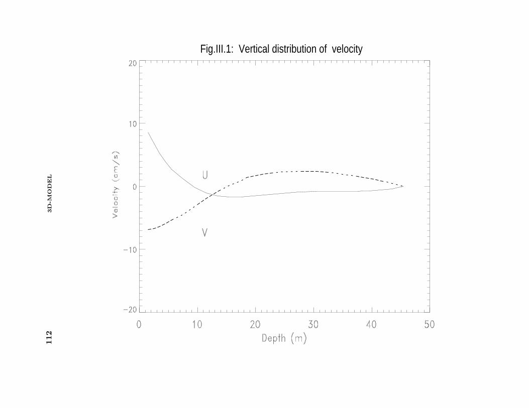
112
3D
-MO
DEL
Fig.III.1: Vertical distribution of velocity

3D-MODEL 113
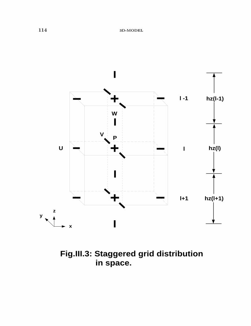
114 3D-MODEL
U
V
W
P
l
l+1
l -1
hz(l)
hz(l-1)
hz(l+1)
y
x
z
Fig.III.3: Staggered grid distribution in space.
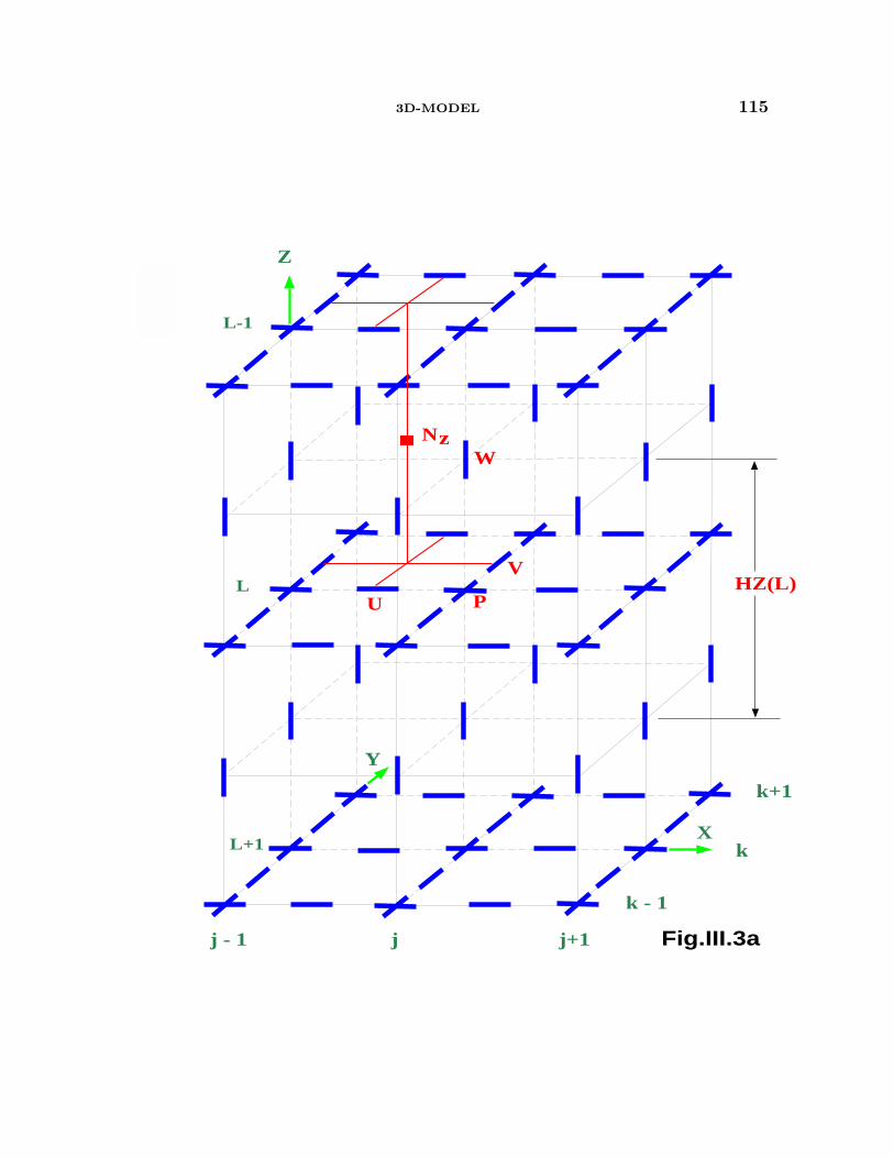
3D-MODEL 115
Nz
U P
V
W
Z
Y
X
j - 1 j j+1
k - 1
k+1
k
l
L
L
L+1
L
L-1
HZ(L)
Fig.III.3a

116 3D-MODEL
Problem No. 2, 3D- barotropic model
To learn basics of 3D-model construction we consider barotropic motion only,i.e., density driven currents will be neglected. Two-time-level numerical schemeswill be used. This approach is delineated in Ch.IV, Sec. 3.2 of NM. To show thearrangement for the time stepping we shall write first the equations of motion alongx and y directions
um+1 − um
T+ (u
∂u
∂x)m + (v
∂u
∂y)m + (w
∂u
∂z)m − fvm
= − 1ρo
∂pa∂x
m
− g∂ζ
∂x
m
+∂
∂zNz
∂u
∂z
m
+ Nh∆um (III.5)
andvm+1 − vm
T+ (u
∂v
∂x)m + (v
∂v
∂y)m + (w
∂v
∂z)m + fum+1
= − 1ρo
∂pa∂y
m
− g∂ζ
∂y
m
+∂
∂zNz
∂v
∂z
m
+ Nh∆vm (III.6)
Construction of the finite-difference equations will be carried out with the help ofFig.III.3 and Fig.III.3a (Fig.4.7 from NM), in which three-dimensional grid distri-bution is shown.
To derive the vertical velocity at any layer l, the equation of continuity isvertically integrated from l + 1 to l,
∫ l
l+1
(∂u
∂x+
∂v
∂y)dz + wm
j,k,l − wmj,k,l+1 = 0
Approximating the above integral as
hz,l(umj+1,k,l − umj,k,l
hx+
vmj,k,l − vmj,k−1,l
hy) + wm
j,k,l − wmj,k,l+1 = 0
the vertical velocity at the l layer becomes
wmj,k,l = wm
j,k,l+1 − hz,l(umj+1,k,l − umj,k,l
hx+
vmj,k,l − vmj,k−1,l
hy) (III.7)
Integration of equation of continuity over the depth yields an additional equa-tion for the unknown sea level,
∂ζ
∂t+
∂
∂x
∫ ζ
−H
udz +∂
∂y
∫ ζ
−H
vdz = 0 (III.8)
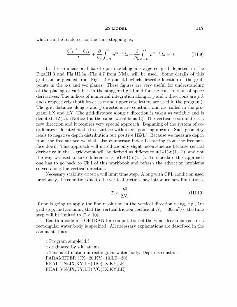
3D-MODEL 117
which can be rendered for the time stepping as,
ζm+1j,k − ζmj,k
T+
∂
∂x
∫ ζ
−H
um+1dz +∂
∂y
∫ ζ
−H
vm+1dz = 0 (III.9)
In three-dimensional barotropic modeling a staggered grid depicted in theFigs.III.3 and Fig.III.3a (Fig 4.7 from NM), will be used. Some details of thisgrid can be gleaned from Figs. 4.8 and 4.1 which describe location of the grid-points in the x-z and y-z planes. These figures are very useful for understandingof the placing of variables in the staggered grid and for the construction of spacederivatives. The indices of numerical integration along x, y and z directions are j, kand l respectively (both lower case and upper case letters are used in the program).The grid distance along x and y directions are constant, and are called in the pro-gram HX and HY. The grid-distance along z direction is taken as variable and isdenoted HZ(L). (Notice l is the same variable as L). The vertical coordinate is anew direction and it requires very special approach. Beginning of the system of co-ordinates is located at the free surface with z axis pointing upward. Such geometryleads to negative depth distribution but positive HZ(L). Because we measure depthfrom the free surface we shall also enumerate index L starting from the free sur-face down. This approach will introduce only slight inconvenience because centralderivative in the L grid-point will be derived as difference u(L-1)-u(L+1), and notthe way we used to take difference as u(L+1)-u(L-1). To elucidate this approachone has to go back to Ch.I of this workbook and refresh the advection problemssolved along the vertical direction.
Necessary stability criteria will limit time step. Along with CFL condition usedpreviously, the condition due to the vertical friction may introduce new limitations.
T <h2z
2Nz(III.10)
If one is going to apply the fine resolution in the vertical direction using, e.g., 1mgrid step, and assuming that the vertical friction coefficient Nz=500cm2/s, the timestep will be limited to T < 10s.
Benith a code in FORTRAN for computation of the wind driven current in arectangular water body is specified. All necessary explanations are described in thecomments lines
c Program simple3d.fc originated by z.k. at imsc This is 3d motion in rectangular water body. Depth is constant.PARAMETER (JX=20,KY=10,LE=30)REAL UN(JX,KY,LE),UO(JX,KY,LE)REAL VN(JX,KY,LE),VO(JX,KY,LE)
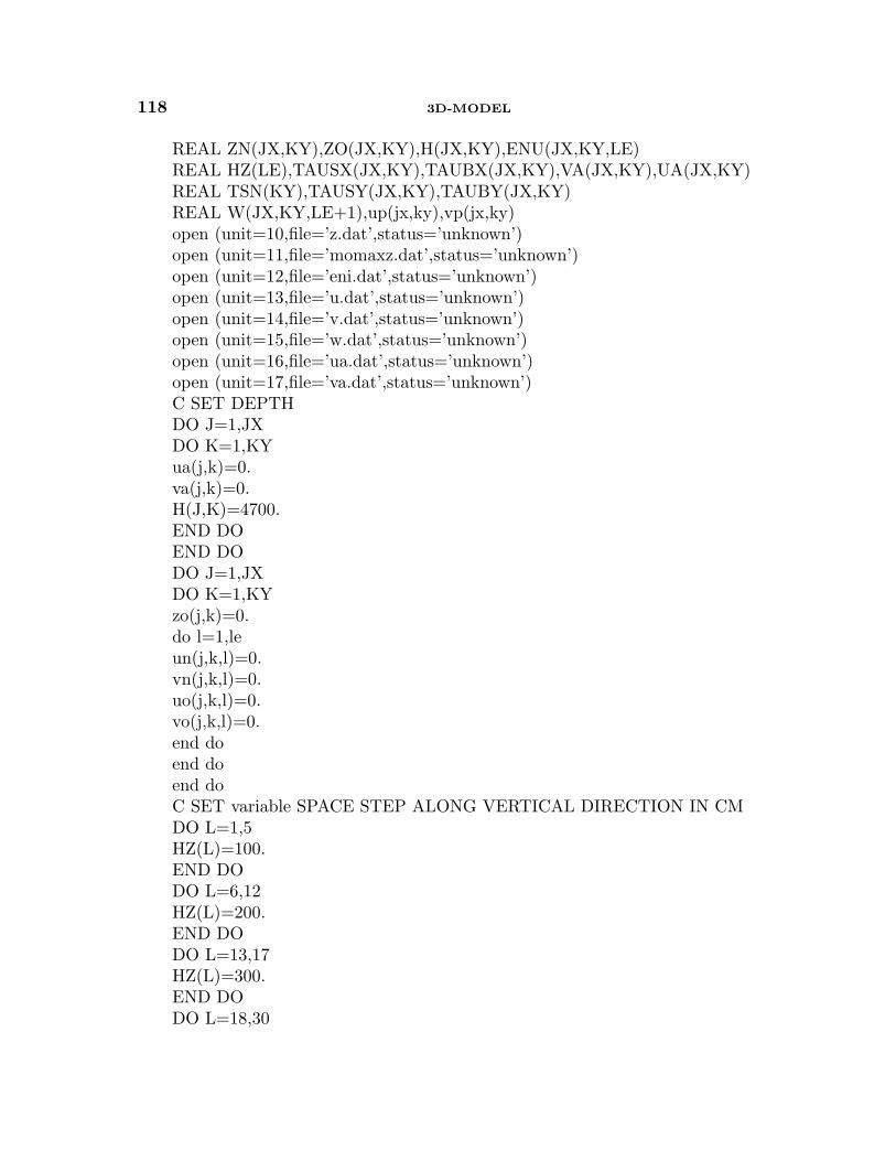
118 3D-MODEL
REAL ZN(JX,KY),ZO(JX,KY),H(JX,KY),ENU(JX,KY,LE)REAL HZ(LE),TAUSX(JX,KY),TAUBX(JX,KY),VA(JX,KY),UA(JX,KY)REAL TSN(KY),TAUSY(JX,KY),TAUBY(JX,KY)REAL W(JX,KY,LE+1),up(jx,ky),vp(jx,ky)open (unit=10,file=’z.dat’,status=’unknown’)open (unit=11,file=’momaxz.dat’,status=’unknown’)open (unit=12,file=’eni.dat’,status=’unknown’)open (unit=13,file=’u.dat’,status=’unknown’)open (unit=14,file=’v.dat’,status=’unknown’)open (unit=15,file=’w.dat’,status=’unknown’)open (unit=16,file=’ua.dat’,status=’unknown’)open (unit=17,file=’va.dat’,status=’unknown’)C SET DEPTHDO J=1,JXDO K=1,KYua(j,k)=0.va(j,k)=0.H(J,K)=4700.END DOEND DODO J=1,JXDO K=1,KYzo(j,k)=0.do l=1,leun(j,k,l)=0.vn(j,k,l)=0.uo(j,k,l)=0.vo(j,k,l)=0.end doend doend doC SET variable SPACE STEP ALONG VERTICAL DIRECTION IN CMDO L=1,5HZ(L)=100.END DODO L=6,12HZ(L)=200.END DODO L=13,17HZ(L)=300.END DODO L=18,30
3D-MODEL 119
HZ(L)=100.END DOC VARIABLE LATITUDE and table for sin tsn(k)pi = 4.*atan(1.)rad = pi/180.ygrid = 1./60. ! ( 1 min : y-axis )blat = 55.+ygridtsN(1) = sin(blat*rad)templat=blatcdo k=2,ky+1templat = templat+ygridtsN(k) = sin(templat*rad)enddoC ALL COEFFICIENTSc=======================================C SET WIND FOR INITIAL EXPERIMENTDO J=1,JXDO K=1,KYTAUSX(J,K)=1.TAUSY(J,K)=0.END DOEND DOc Time stepT = 10.c HORIZONTAL EDDY VISCOSITYAH=1.0e7G=981.c SPACE STEPS ALONG X AND YHY=13.89E5HX=13.89E5FC=1.458E-4RF1=2.6E-3C COMBINATIONAL PARAMETERSTRF=T*RF1PL=T/HXGPL=G*PLPLL=AH*T/(HX*HX)PF=T/HYGPF=G*PFPFF=AH*T/(HY*HY)TFC=T*FC
120 3D-MODEL
C START TIME LOOP INDEX N RUNS UNTIL N=MONc*******************************MON=86400C888888888888888888888888888888850 N=N+1C SET WIND FOR INITIAL EXPERIMENTDO J=1,JXDO K=1,KYTAUSX(J,K)=1.TAUSY(J,K)=0.END DOEND DOc if (n.lt.1000)thenc DO J=1,JXc DO K=1,KYc TAUSX(J,K)=float(n)/1000.c TAUSY(J,K)=0.c END DOc END DOc end ifC EDDY VISCOSITY IS CONSTANTDO 33J=1,JXDO 33K=1,KYDO 33 L=1,LeENU(J,K,L)=50.33 CONTINUEC COMPUTATION OF U VELOCITYDO 4 J=3,JX-2DO 4 K=2,KY-1C SURFACE CONDITIONUAV=0.25*(VO(J-1,K,1)+VO(J-1,K-1,1)+VO(J,K-1,1)+VO(J,K,1))DSL=ZO(J,K)-ZO(J-1,K)DSLX=GPL*DSLHZP=0.5*(HZ(1)+HZ(2))DSU=(UO(J,K,1)-UO(J,K,2))/HZPVFRS=(TAUSX(J,K)-ENU(J,K,2)*DSU)/HZ(1)HFR=PLL*(UO(J+1,K,1)+UO(J-1,K,1)-2.*UO(J,K,1))+2PFF*(UO(J,K+1,1)+UO(J,K-1,1)-2.*UO(J,K,1))C NONLINEAR TERMSQ1=0.5*(UAV+ABS(UAV))Q2=0.5*(UAV-ABS(UAV))ONHY1=PF*Q1*(UO(J,K,1)-UO(J,K-1,1))
3D-MODEL 121
ONHY2=PF*Q2*(UO(J,K+1,1)-UO(J,K,1))Q3=0.5*(UO(J,K,1)+ABS(UO(J,K,1)))Q4=0.5*(UO(J,K,1)-ABS(UO(J,K,1)))ONH1=PL*Q3*(UO(J,K,1)-UO(J-1,K,1))ONH2=PL*Q4*(UO(J+1,K,1)-UO(J,K,1))SUMNONX=ONH1+ONH2+ONHY1+ONHY2UN(J,K,1)=UO(J,K,1)+TFC*UAV*TSN(K)-DSLX+VFRS*T+HFR-2SUMNONXLMM=LE-1DO 5 L=2,LMM-1UAV=0.25*(VO(J-1,K,L)+VO(J-1,K-1,L)+VO(J,K-1,L)+VO(J,K,L))HZP=0.5*(HZ(L)+HZ(L+1))HZN=0.5*(HZ(L)+HZ(L-1))DSUN=(UO(J,K,L-1)-UO(J,K,L))/HZNDSUP=(UO(J,K,L)-UO(J,K,L+1))/HZPVFR=(ENU(J,K,L)*DSUN-ENU(J,K,L+1)*DSUP)/HZ(L)HFR=PLL*(UO(J+1,K,L)+UO(J-1,K,L)-2.*UO(J,K,L))+2PFF*(UO(J,K+1,L)+UO(J,K-1,L)-2.*UO(J,K,L))C NONLINEAR TERMSQ1=0.5*(UAV+ABS(UAV))Q2=0.5*(UAV-ABS(UAV))ONHY1=PF*Q1*(UO(J,K,L)-UO(J,K-1,L))ONHY2=PF*Q2*(UO(J,K+1,L)-UO(J,K,L))Q3=0.5*(UO(J,K,L)+ABS(UO(J,K,L)))Q4=0.5*(UO(J,K,L)-ABS(UO(J,K,L)))ONH1=PL*Q3*(UO(J,K,L)-UO(J-1,K,L))ONH2=PL*Q4*(UO(J+1,K,L)-UO(J,K,L))SUMNONX=ONH1+ONH2+ONHY1+ONHY2UN(J,K,L)=UO(J,K,L)+TFC*UAV*TSN(K)-DSLX+VFR*T+HFR-2SUMNONX5 CONTINUEC BOTTOM CONDITION GIVEN BOTTOM STRESSUAV=0.25*(VO(J-1,K,LMM)+VO(J-1,K-1,LMM)2+VO(J,K-1,LMM)+VO(J,K,LMM))HZP=HZ(LMM)HZN=0.5*(HZ(LMM)+HZ(LMM-1))DSUP=2.*UO(J,K,LMM)/HZPDSUN=(UO(J,K,LMM-1)-UO(J,K,LMM))/HZNc VFR=(ENU(J,K,LMM)*DSVN-ENU(J,K,LMM+1)*DSUP)/HZ(LMM)PIERW=SQRT(UAV*UAV+UO(J,K,LMM)*UO(J,K,LMM))TAUBX(J,K)=TRF*PIERW*UO(J,K,LMM)VFR=(ENU(J,K,LMM)*DSUN-TAUBX(J,K))/HZ(LMM)

122 3D-MODEL
HFR=PLL*(UO(J+1,K,LMM)+UO(J-1,K,LMM)-2.*UO(J,K,LMM))+2PFF*(UO(J,K+1,LMM)+UO(J,K-1,LMM)-2.*UO(J,K,LMM))C NONLINEAR TERMSQ1=0.5*(UAV+ABS(UAV))Q2=0.5*(UAV-ABS(UAV))ONHY1=PF*Q1*(UO(J,K,LMM)-UO(J,K-1,LMM))ONHY2=PF*Q2*(UO(J,K+1,LMM)-UO(J,K,LMM))Q3=0.5*(UO(J,K,LMM)+ABS(UO(J,K,LMM)))Q4=0.5*(UO(J,K,LMM)-ABS(UO(J,K,LMM)))ONH1=PL*Q3*(UO(J,K,LMM)-UO(J-1,K,LMM))ONH2=PL*Q4*(UO(J+1,K,LMM)-UO(J,K,LMM))SUMNONX=ONH1+ONH2+ONHY1+ONHY2UN(J,K,LMM)=UO(J,K,LMM)+TFC*UAV*TSN(K)-DSLX+VFR*T+HFR-2SUMNONXUN(J,K,LMM)=0.4 CONTINUEC COMPUTATION OF V VELOCITYDO 6 J=2,JX-1DO 6 K=3,KY-2C SURFACE CONDITIONVAUN=0.25*(UN(J,K,1)+UN(J,K+1,1)+UN(J+1,K,1)+UN(J+1,K+1,1))DSL=ZO(J,K+1)-ZO(J,K)DSLY=GPF*DSLHZP=0.5*(HZ(1)+HZ(2))DSV=(VO(J,K,1)-VO(J,K,2))/HZPVFRS=(TAUSY(J,K)-ENU(J,K,2)*DSV)/HZ(1)HFR=PLL*(VO(J+1,K,1)+VO(J-1,K,1)-2.*VO(J,K,1))+2PFF*(VO(J,K+1,1)+VO(J,K-1,1)-2.*VO(J,K,1))C COMPUTING NONLINEAR TERMSVAU=0.25*(UO(J,K,1)+UO(J,K+1,1)+UO(J+1,K,1)+UO(J+1,K+1,1))Q1=0.5*(VAU+ABS(VAU))Q2=0.5*(VAU-ABS(VAU))ONHX1=PL*Q1*(VO(J,K,1)-VO(J-1,K,1))ONHX2=PL*Q2*(VO(J+1,K,1)-VO(J,K,1))Q3=0.5*(VO(J,K,1)+ABS(VO(J,K,1)))Q4=0.5*(VO(J,K,1)-ABS(VO(J,K,1)))ONHY1=PF*Q3*(VO(J,K,1)-VO(J,K-1,1))ONHY2=PF*Q4*(VO(J,K+1,1)-VO(J,K,1))SUMNONY=ONHX1+ONHX2+ONHY1+ONHY2VN(J,K,1)=VO(J,K,1)-TFC*VAUN*TSN(K)-DSLY+VFRS*T+HFR-2SUMNONYLMM=LE-1
3D-MODEL 123
DO 7 L=2,LMM-1VAUN=0.25*(UN(J,K,L)+UN(J,K+1,L)+UN(J+1,K,L)+UN(J+1,K+1,L))HZP=0.5*(HZ(L)+HZ(L+1))HZN=0.5*(HZ(L)+HZ(L-1))DSVN=(VO(J,K,L-1)-VO(J,K,L))/HZNDSVP=(VO(J,K,L)-VO(J,K,L+1))/HZPVFR=(ENU(J,K,L)*DSVN-ENU(J,K,L+1)*DSVP)/HZ(L)HFR=PLL*(VO(J+1,K,L)+VO(J-1,K,L)-2.*VO(J,K,L))+2PFF*(VO(J,K+1,L)+VO(J,K-1,L)-2.*VO(J,K,L))C COMPUTING NONLINEAR TERMSVAU=0.25*(UO(J,K,L)+UO(J,K+1,L)+UO(J+1,K,L)+UO(J+1,K+1,L))Q1=0.5*(VAU+ABS(VAU))Q2=0.5*(VAU-ABS(VAU))ONHX1=PL*Q1*(VO(J,K,L)-VO(J-1,K,L))ONHX2=PL*Q2*(VO(J+1,K,L)-VO(J,K,L))Q3=0.5*(VO(J,K,L)+ABS(VO(J,K,L)))Q4=0.5*(VO(J,K,L)-ABS(VO(J,K,L)))ONHY1=PF*Q3*(VO(J,K,L)-VO(J,K-1,L))ONHY2=PF*Q4*(VO(J,K+1,L)-VO(J,K,L))SUMNONY=ONHX1+ONHX2+ONHY1+ONHY2VN(J,K,L)=VO(J,K,L)-TFC*VAUN*TSN(K)-DSLY+VFR*T+HFR-2SUMNONY7 CONTINUEC BOTTOM CONDITION GIVEN BOTTOM STRESS OR VELOCITYC GOES TO ZEROVAUN=0.25*(UN(J,K,LMM)+UN(J,K+1,LMM)2+UN(J+1,K,LMM)+UN(J+1,K+1,LMM))HZP=HZ(LMM)HZN=0.5*(HZ(LMM)+HZ(LMM-1))DSVN=(VO(J,K,LMM-1)-VO(J,K,LMM))/HZNDSVP=2.*VO(J,K,LMM)/HZPPIERW=SQRT(VAUN*VAUN+VO(J,K,LMM)*VO(J,K,LMM))TAUBY(J,K)=TRF*PIERW*VO(J,K,LMM)VFR=(ENU(J,K,LMM)*DSVN-TAUBY(J,K))/HZ(LMM)C VFR=(ENU(J,K,LMM)*DSVN-ENU(J,K,LMM+1)*DSVP)/HZ(LMM)HFR=PLL*(VO(J+1,K,LMM)+VO(J-1,K,LMM)-2.*VO(J,K,LMM))+2PFF*(VO(J,K+1,LMM)+VO(J,K-1,LMM)-2.*VO(J,K,LMM))C COMPUTING NONLINEAR TERMSVAU=0.25*(UO(J,K,LMM)+UO(J,K+1,LMM)+UO(J+1,K,LMM)2+UO(J+1,K+1,LMM))Q1=0.5*(VAU+ABS(VAU))Q2=0.5*(VAU-ABS(VAU))

124 3D-MODEL
ONHX1=PL*Q1*(VO(J,K,LMM)-VO(J-1,K,LMM))ONHX2=PL*Q2*(VO(J+1,K,LMM)-VO(J,K,LMM))Q3=0.5*(VO(J,K,LMM)+ABS(VO(J,K,LMM)))Q4=0.5*(VO(J,K,LMM)-ABS(VO(J,K,LMM)))ONHY1=PF*Q3*(VO(J,K,LMM)-VO(J,K-1,LMM))ONHY2=PF*Q4*(VO(J,K+1,LMM)-VO(J,K,LMM))SUMNONY=ONHX1+ONHX2+ONHY1+ONHY2VN(J,K,LMM)=VO(J,K,LMM)-TFC*VAUN*TSN(K)-DSLY+VFR*T+HFR-2SUMNONYVN(J,K,LMM)=0.6 CONTINUEC SEA LEVELC FIRST AVERAGE VELOCITY ALONG VERTICAL DIRECTIONc print *, un(2,5,1),un(3,5,1)DO 9 J=3,JX-2DO 9 K=2,KY-1MM=LEC++++++++++++++++++++++++++++++++++++++++++HZ(1)=100.+(ZO(J,K)+ZO(J-1,K))*0.5UA(J,K)=0.HZS=0.DO 10 L=MM,1,-1UA(J,K)=UA(J,K)+UN(J,K,L)*HZ(L)HZS=HZS+HZ(L)10 CONTINUEc if (ua(j,k).gt.11) print *, j,kc IN CASE YOU NEED AVERAGE VELOCITYc UAR(J,K)=UA(J,K)/HZS9 CONTINUEc****************************************c print *, UA(2,5),UA(3,5)DO 11 J=2,JX-1DO 11 K=3,KY-2C+++++++++++++++++++++++++++++++++++++++++HZ(1)=100.+(ZO(J,K)+ZO(J,K+1))*0.5MM=LEVA(J,K)=0.HZS=0.DO 12 L=MM,1,-1VA(J,K)=VA(J,K)+VN(J,K,L)*HZ(L)HZS=HZS+HZ(L)12 CONTINUE
3D-MODEL 125
c VAR(J,K)=VA(J,K)/HZS11 CONTINUEC NOW USE CONTINUITY EQUATIONc LZ=0DO 13 J=2,JX-1DO 13 K=2,KY-1c93 CONTINUEZN(J,K)=ZO(J,K)-PL*(UA(J+1,K)-UA(J,K))-PF*(VA(J,K)-VA(J,K-1))c LZ=LZ+1c IF(LZ.EQ.2)THENc LZ=0c ZS(J,K)=ZO(J,K)c GO TO 13c END IFc ZO(J,K)=0.25*ZN(J,K)+0.5*ZO(J,K)+0.25*ZS(J,K)c GO TO 9313 CONTINUEc vertical velocity from continuity equationHZ(1)=100+ZO(J,K)DO 25 J=2,JX-1DO 25 K=2,KY-1MLEZ=LEW(J,K,MLEZ+1)=0.DO 26 L=1,MLEZHZX=HZ(L)/HXHZY=HZ(L)/HYDIFU=UN(J+1,K,L)-UN(J,K,L)DIFV=VN(J,K,L)-VN(J,K-1,L)W(J,K,L)=W(J,K,L+1)-HZX*DIFU-HZY*DIFV26 CONTINUE25 CONTINUEC CHANGE VARIABLESDO 15 J=1,JXDO 15 K=1,KYDO 15L=1,LEUO(J,K,L)=UN(J,K,L)VO(J,K,L)=VN(J,K,L)15 CONTINUEdo J=1,JXDO K=1,KYzo(j,k)=zn(j,k)end do

126 3D-MODEL
end doc print *, ua(10,10),ua(19,10)c print *, un(10,5,1),un(10,5,2),un(10,5,3)c print *, vn(10,5,1),vn(10,5,2),vn(10,5,3)c print *, zn(3,5),zn(10,5),zn(18,5)c print *, ’zn(3,5)’,’ua(4,5)’,’ua(3,5)’,’zo(3,5)’c print *,’va(3,5)’,’va(3,4)’if(mod(N,200).eq.0) thenC THIS FOR THE VERTICALLY AVERAGE FLOWc Computing kinetic and potential energy every 200 stepsc ENI enrgy every 180 steps , averaged over whole spaceNC=N/200ES=0.do j=1,JX-1do k=2,KYuaE=0.5*(ua(j,k)+ua(j+1,k))vaE=0.5*(va(j,k)+va(j,k-1))en=(uaE*uaE+vaE*vaE)/(2.*g*h(j,k))+zn(j,k)*zn(j,k)/2.es=en+esend doend doc eni(nc)=eswrite(12,*)eswrite(11,*),n,zn(2,5),zn(10,5),zn(18,5)print *,n,’zn(2,5)=’,zn(2,5),’zn(10,5)=’,zn(10,5)print *,’zn(18,5)=’,zn(18,5)end ifIF(N.LT.MON)GO TO 50c WRITE SEA LEVEL AND VELOCITIESWRITE(10,*)((ZN(J,K),J=1,JX),K=1,KY)Do j=1,jxdo k=1,kyup(j,k)=0.5*(un(J,K,1)+un(j+1,k,1))vp(j,k)=0.5*(vn(j,k-1,1)+vn(J,K,1))end doend doWRITE(16,*)((up(j,k),J=1,JX),K=1,KY)WRITE(17,*)((vp(j,k),J=1,JX),K=1,KY)DO L=1,LEuw=(Un(9,5,L)+Un(10,5,L))*0.5WRITE(13,*)(uw)END DO
3D-MODEL 127
DO L=1,LEvw=(Vn(9,5,L)+Vn(9,4,L))*0.5WRITE(14,*)vwEND DOc DO L=1,LEc WRITE(15,*)((w(J,K,L),J=1,JX),K=1,KY)c END DOstopend
Some results of computations are given in figs. III.4, III.5 and III.6. Fig.III.4depicts temporal changes of the sea level at the three locations along x directions.Because wind is directed along x axis the sea level will increase along the sameaxis. Periodical oscillations of the sea level are defined by own oscillations of thewater body, or seiche. After about 4 day of the process a steady state occurs. InFig.III.5 a vertical distribution of the horizontal current is depicted. The point forthis distribution is located at the center of the rectangular water body. Comparingthis distribution with distribution from Fig.III.1 one can see both similar and dis-similar behavior. This is caused by the presence of the slope current in the lattercomputations. In fig.III.6 calculated current at the surface is given after about fourdays of process.

128
3D
-MO
DEL
Fig.III.4: Sea Level
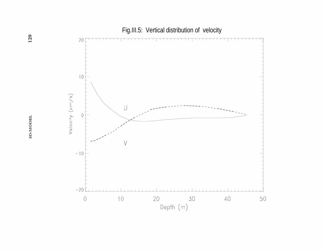
3D
-MO
DEL
129
Fig.III.5: Vertical distribution of velocity

130
3D
-MO
DEL
Fig.III.5: Rectangular water body
0 5 10 15Wind driven current,tx=1
0
2
4
6
8
19.7195 cm/s
66 6

3D-MODEL AND SIGMA COORDINATE 131
Problem No. 3, 3D- barotropic model, sigma coordinate
Introduction
The modeling of the oceanic flow in the so-called sigma coordinate requires achange from the regular, everyday prospective into the one with the vertical coordi-nate stretched thus vertical distance is expressed in relation to the total depth. Thisapproach is similar to application of percentage. The total depth instead of 100%is equal to 1. This approach, presumably simple, requires a lot of changing in theequations and in the programming. Let assume the total depth is 100 m and thatthe measurements of temperature were done at the irregular depth intervals. Thesedata can not be taken as an initial data for the sigma model, they must be trans-ferred into sigma coordinate by approximating values from the regular coordinatesystem, and vice versa, the model results obtained in the sigma coordinate are verydifficult to analyze and to understand, therefore, one must plot data in regular zcoordinate system. The sigma coordinate, or so-called stretching coordinate definesthe new vertical coordinate as
σ =z − ζ
H + ζ(III.11)
The total depth D = H + ζ. The new coordinate transforms entire water columninto a unit depth. The depth in sigma coordinate is changing from 0, at the freesurface to −1 at the bottom. (Fig. 4.10 from (NM) explains applications of thesigma coordinate and its relation to z coordinate system). Relations between oldand new coordinates and derivatives in the new system of coordinate are given inNM Ch. 4, section 4.3. A set of equations of motion and continuity in the newindependent variables (x, y, σ, t) is given below:
∂
∂t(uD) +
∂
∂x(u2D) +
∂
∂y(uvD) +
∂
∂σ(Wu) − fDv
= −gD∂ζ
∂x+
1D
∂
∂σ(Nz
∂u
∂σ) + +Nh[
∂
∂xD
∂u
∂x+
∂
∂yD
∂u
∂y] (III.12)
∂
∂t(vD) +
∂
∂x(uvD) +
∂
∂y(v2D) +
∂
∂σ(Wv) + fDu
= −gD∂ζ
∂y+
1D
∂
∂σ(Nz
∂v
∂σ) + Nh[
∂
∂xD
∂v
∂x+
∂
∂yD
∂v
∂y] (III.13)
∂ζ
∂t+
∂
∂x(uD) +
∂
∂y(vD) +
∂
∂σ(W ) = 0 (III.14)
In the above equations W is the vertical velocity in the new system of coordi-nate. It is defined by eq. (4.178) from NM. The relation between the old verticalvelocity w and the new one is defined as

132 3D-MODEL AND SIGMA COORDINATE
W = w − (σ + 1)∂ζ
∂t− uQx − vQy (III.15)
Here
W = DDσ
Dt, Qx = σ
∂D
∂x+
∂ζ
∂x, Qy = σ
∂D
∂y+
∂ζ
∂y(III.16)
Boundary conditions for the vertical velocity at the free surface and at the bottom(eqs. 1.64 and 1.65 a from NM) change in the new system of coordinate to:
W (x, y, 0, t) = 0 W (x, y,−1, t) = 0 (III.17)
Boundary conditions at the surface and at the bottom are defined by horizontalstresses
τ sx =ρNz
D
∂u
∂στ sy =
ρNz
D
∂v
∂σat σ = 0 (III.17a)
τ bx =ρNz
D
∂u
∂στ by =
ρNz
D
∂v
∂σat σ = −1 (III.17b)
Integrating eq.(III.14) with respect to σ and applying the boundary condition ex-pressed by eq.(III.17) we arrive at the vertically integrated continuity equation(eq.4.182b from NM),
∂
∂x(uD) +
∂
∂y(vD) +
∂ζ
∂t= 0 (III.18)
The components of the depth-averaged velocity in the above equation are expressedas
u =∫ 0
−1
udσ v =∫ 0
−1
vdσ (III.19)
How to write code in the nonrectangular domain
Let us consider water body that has circular shape in the horizontal plain.Its bathymetry is defined by parabolic function. Rectangular system of coordinatechanges along x direction from x=0 to x=200 km and in similar fashion along they direction. Space step of numerical integration is 10km. General equation for thedepth reads
z = −a(x2 + y2) + c (III.20)
Ensuing FORTRAN program prescribes depth according to the above equation.Depth is given in the positive numbers (cm).
C Program depthdat.fC PROGRAM TO PRESCRIBE DEPTH IN CIRCULAR BASIN
3D-MODEL AND SIGMA COORDINATE 133
PARAMETER (JX=21,KY=21)REAL H(JX,KY)open (unit=1,file=’parab.dat’,status=’unknown’)DO J=1,JXDO K=1,KYHXD=((Float(j)-1.)*0.1-1.)*((Float(j)-1.)*0.1-1.)HYD=((Float(K)-1.)*0.1-1.)*((Float(K)-1.)*0.1-1.)c the maximum depth is 13000 cmH(j,K)=-4500.*3.*(HXD+HYD)+13000.c at any location where depth is less or equal 500cm the depth isc set to zero. So that insidec computational domain only depth greater than 500cm will occur.if(h(j,k).le.500.)h(j,k)=0.END DOEND DOwrite(1,*)((h(j,k),j=1,jx),k=1,ky)stopend
To describe 3-D time dependent motion we shall solve eq. III.12, III.13, III.14and III.18. Numerical solution will proceed separately for the u, v,W and for thesea level ζ. These equations are to be solved in the staggered grid shown in Fig.III.3(Fig.4.7 from NM). A good approach is to organize numerical solution along thehorizontal and vertical lines. We shall first explain organization of computation inthe horizontal direction, i.e. at the u and v grid points, because code along thevertical direction is quite similar to the solution in z coordinate. The importantconsequence of the sigma coordinate application (which can be easily deduced fromthe Fig. 4.10 of NM) is that number of grid points along the vertical direction (i. e.,number of layers) is always the same at each location. This is not the case for thez coordinate. Due to assumption of a constant layer thickness in z coordinate thenumber of grid points along the vertical direction will be greater at the greater depthand smaller at the smaller depth. Because each layer in sigma coordinate occursthroughout the entire horizontal domain, one can conclude that sigma coordinate isanalogous to the vertically averaged set of equations. Therefore, grid distributionand enumeration along the horizontal direction for the sigma coordinate modelis similar to the vertically averaged model. For the irregular water bodies it isimportant to differentiate between greed points located over water and over dryland. The number of grid points over water along each column and row is variabledue to variable coastline.
In irregular water bodies we first learn how to enumerate the grid points whichare located in water. The explanation of such procedure is given on p. 134 of NM.We shall explore first this procedure to establish the set of indices for the horizontal
134 3D-MODEL AND SIGMA COORDINATE
u velocity computation. Thus checking each row from k=1 to k=ky, one can locateat each row starting point (js) and ending point (je) of the water domain. Thedepth of land and coastal line is set to zero. Because of islands it may happen thatin some rows to each k a few different starting and ending points will be prescribed.This is done in the program by counting the number of segments. An individualsegment in the program is called, a line. Proceeding in similar way from the firstcolumn (j=1) to the last column (j=jx), one can establish beginning and endingindices for the v velocity integration along the y direction. This is all done in theFORTRAN program named index.f. This program reads depth distribution fromthe file parab.dat and outputs indices for the u and v integration. It also calculatesthe number of lines along the x and y direction, therefore every set of indices canbe related to the proper line number.
c PROGRAM ORIGINATED BY DOKUY LEE FROM IOS, VICTORIAparameter (jx=21,ky=21)dimension dep(jx,ky)open (unit=1,file=’parab.dat’,status=’unknown’)open (4,file=’parab.ind’)read(1,*)((dep(j,k),j=1,JX),k=1,ky)c set around your domain zero., because program senses zeroc and non zero depthc to establish starting and ending index for the horizontal andc vertical lines.do j=1,jxdep(j,1) = 0.dep(j,2)=0.c dep(j,3)=0.enddocdo j=1,jxdep(j,ky) = 0.dep(j,ky-1) = 0c dep(j,ky-2)=0.enddocdo k=1,kydep(1,k) = 0.dep(2,k)=0.c dep(3,k)=0.enddocdo k=1,ky

3D-MODEL AND SIGMA COORDINATE 135
dep(jx,k) = 0dep(jx-1,k)=0.c dep(jx-2,k)=0.enddocwrite(4,101)101 format(’ Begining of horizontal’)csum=0 ! sum give the total number of horizontal and vertical lines.ih = 0 ! ih will tell how many horizontal lines have depthdo k=1,ky ! k stands for the row numberifirst = 0 !this index helps to recognize line’s beginning and enddo j=1,jxif(dep(j,k).gt.0.0.and.ifirst.eq.0) thenjs = jifirst = 1endifif(dep(j,k).le.0.0.and.ifirst.eq.1) thenje = j-1ifirst = 0sum=sum+1write(4,100) k,k,js,je100 format(4i4)ih = ih+1endifenddoenddoc write(*,*)sumwrite(4,102)102 format(’ Begining of vertical’)civ = 0 ! this will tell how many vertical linesdo j=1,jxifirst = 0do k=1,kyif(dep(j,k).gt.0.0.and.ifirst.eq.0) thenks = kifirst = 1endifif(dep(j,k).le.0.0.and.ifirst.eq.1) thenke = k-1ifirst = 0
136 3D-MODEL AND SIGMA COORDINATE
sum=sum+1c write(6,100) j,j,ks,kewrite(4,100) j,j,ks,keiv = iv+1endifenddoenddowrite(*,*)ih,iv,sumstopend
The output from the above program written to the file parab.ind isgiven below. There are 17 lines along horizontal and 17 lines along verticaldirections. Along the horizontal direction first two indices denote rownumber,for example 3 3, stands for the third row. The js=6 and je=16 denotesbeginning and end of integration for the u velocity in the third row.Similar approachis taken for the v velocity (vertical lines). Here first two indices denotecolumn number, for example 3 3 stands for the third column (j=3).Calculation of v in this column is done from ks=6 to ke=16.
3 3 6 16 Begining of horizontal4 4 5 175 5 4 186 6 3 197 7 3 198 8 3 199 9 3 1910 10 3 1911 11 3 1912 12 3 1913 13 3 1914 14 3 1915 15 3 1916 16 3 1917 17 4 1818 18 5 1719 19 6 163 3 6 16 Begining of vertical4 4 5 175 5 4 186 6 3 19
3D-MODEL AND SIGMA COORDINATE 137
7 7 3 198 8 3 199 9 3 1910 10 3 1911 11 3 1912 12 3 1913 13 3 1914 14 3 1915 15 3 1916 16 3 1917 17 4 1818 18 5 1719 19 6 16
As we know how to enumerate variable domain in the horizontal plane let’sconstruct numerical form of the system of equation of motion and continuity in thesigma coordinate. We start by considering the time differencing. A two-time-levelscheme will be used for the equations of motion along x and y direction (eqs.III.12,III.13)
(uD)m∗ − (uD)m
T+
∂
∂x(u2D)m +
∂
∂y(uvD)m +
∂
∂σ(Wu)m − f(Dv)m
= −gDm(∂ζ
∂x)m + Nh[
∂
∂xDm ∂um
∂x+
∂
∂yDm ∂um
∂y] (III.21a)
(uD)m+1 − (uD)m∗
T=
1Dm
∂
∂σ(Nz
∂u
∂σ)m+1 (III.21b)
(vD)m∗ − (vD)m
T+
∂
∂x(uvD)m +
∂
∂y(v2D)m +
∂
∂σ(Wv)m + f(Du)m+1
= −gDm(∂ζ
∂y)m + Nh[
∂
∂xDm ∂vm
∂x+
∂
∂yDm ∂vm
∂y] (III.22a)
(vD)m+1 − (vD)m∗
T=
1Dm
∂
∂σ(Nz
∂v
∂σ)m+1 (III.22b)
The time differencing in the above equations is split into two substeps. The firstsubstep, from m to m∗, uses an explicit scheme to compute intermediate value ofvelocity. (Notice that in eq.III.22a Coriolis force is implicit). At the second substep(marching from m∗ to m+1) an implicit scheme is used to calculate vertical frictionterms. This is done in anticipation of the stability problems which can be caused by

138 3D-MODEL AND SIGMA COORDINATE
the vertical friction (Nz). In the sigma coordinate the layer thickness at the shallowwater regions is significantly reduced, therefore stability condition (p. 62 from NM)requires small time step of numerical integration, possibly even smaller than theCFL condition. The physics of the vertical exchange of momentum can exacerbateproblem as well, because the vertical eddy viscosity can change over the wide rangeof values, again setting restrictions on the time step used in computations.
Space differencing wil be done with the help of staggered grid. It is useful tonotice that the total depth is defined in the ζ points, while above equations requirethe depth in the u and v points as well. Therefore, in the FORTRAN program twoimportant magnitudes HU and HV are introduced. They define the average depthin the u and v points. Denoting the grid point indices as j, k (see Fig.4.7 from NM),the average depth reads,
HU(j, k) = 0.5 ∗ (D(j, k) + D(j − 1, k)) HV (j, k) = 0.5 ∗ (D(j, k) + D(j, k + 1))(III.23)
Part of the total depth is variable in time, therefore the new values are com-puted at every time step. They are called HUN and HVN.
Let’s consider time derivative for the u velocity and its interaction with thetotal depth. It is useful to notice that the values at the m∗ step are intermediatevalues and these do not require the knowledge of the total depth. Thus,
(uD)m+1 − (uD)m
T=
HUNj,k ∗ um+1j,k,l −HUj,k ∗ umj,k,l
T(III.24)
Horizontal derivative of advective terms can be constructed in many differentways. Our aim is to achieve second order of approximation in space. Consider term∂∂x
(u2D)m. (Inner product is composed of two terms uD and u). Approach takenhere is to find an average value of each term at the ζ points which surround u pointand afterwards take difference for the derivative. These ζ points are indexed by j, kand j − 1, k respectively. At the right ζ grid point
(uD)r = 0.5 ∗ (HUj+1,k ∗ uj+1,k,l + HUj,k ∗ uj,k,l) ur = 0.5 ∗ (uj,k,l + uj+1,k,l)(III.25a)
At the left ζ grid-point the above terms change to:
(uD)l = 0.5 ∗ (HUj−1,k ∗ uj−1,k,l + HUj,k ∗ uj,k,l) ul = 0.5 ∗ (uj,k,l + uj−1,k,l)(III.25b)
From these two expressions, the finite difference of the first advective termfollows
∂
∂x(u2D)m � (uD)r ∗ ur − (uD)l ∗ ul
hx(III.25)

3D-MODEL AND SIGMA COORDINATE 139
To conceive above expression we used quite a few averaging operations. It isalways a good idea to pose and to ask what is the meaning of such operations. Wehave enough knowledge to conclude that averaging in proximity to the given gridpoint is equivalent to filtering out some of the short waves. This procedure increasesstability of numerical form. To learn what actually happened some numerical ex-periments are advised, let’s say using staggered grid and grid in which velocitiesand sea level are located at the same grid-point.
Let’s continue with the numerical construction of the advective terms. Deriva-tive ∂
∂y (uvD)m is taken along the y direction, therefore all variables will be locatedup and down of the point uj,k. At the upper location the two terms are considered
(vD)up = 0.5 ∗ (HVj,k ∗ vj,k,l + HVj−1,k ∗ vj−1,k,l) uup = 0.5 ∗ (uj,k,l + uj,k+1,l)(III.26a)
and in the similar way at the lower location
(vD)dw = 0.5 ∗ (HVj,k−1 ∗ vj,k−1,l + HVj−1,k−1 ∗ vj−1,k−1,l)
udw = 0.5 ∗ (uj,k,l + uj,k−1,l) (III.26b)
From these expression the derivative is expressed as,
∂
∂y(uvD)m � (vD)up ∗ uup − (vD)dw ∗ udw
hy(III.26)
The third nonlinear term, a convective transport ∂∂σ (Wu)m, requires differenc-
ing along the vertical direction. One has to construct derivative based on the valuesabove and below u grid point. Again, since W is not located above u grid, butabove pressure grid, the averaging is the order of the day. At the location aboveuj,k,l grid point
Wa = 0.5 ∗ (Wj,k,l + Wj−1,k,l)
ua = (uj,k,l−1 ∗ hzl + uj,k,l ∗ hzl−1)/(hzl + hzl−1) (III.27a)
Wb = 0.5 ∗ (Wj,k,l+1 + Wj−1,k,l+1)
ub = (uj,k,l ∗ hzl+1 + uj,k,l+1 ∗ hzl)/(hzl + hzl+1) (III.27b)
The vertical grid step hzl is chosen to be variable, therefore above averagingprocedure for the u velocity uses weighted averages.
From III.27 a,b the derivative for the convective term follows:
140 3D-MODEL AND SIGMA COORDINATE
∂
∂σ(Wu)m � ua ∗Wa − ub ∗Wb
hzl(III.27)
The Coriolis term along the x direction requires averaging of v component tothe u grid point, concomitantly the total depth is also averaged. The followingformulas are used
vr = 0.5(vj,k,l + vj,k−1,l) vl = 0.5 ∗ (vj−1,k,l + vj−1,k−1,l) (III.28a)
f(Dv)m = f ∗ 0.5 ∗ (Dj,k ∗ vr + Dj−1,k ∗ vl) (III.28)
Note that vr and vl are defined at the pressure (or depth) grid points.To render numerical form for the sea level and horizontal friction terms we use
previous numerical formulas with the small change due to the total depth term.
gDm(∂ζ
∂x)m = g ∗HUj,k ∗ ζj,k − ζj−1,k
hx(III.29)
Nh∂
∂xDm ∂um
∂x� Nh
(hx)2[uj+1,k,l ∗Dj,k + uj−1,k,l ∗Dj−1,k − uj,k,l ∗ (Dj,k + Dj−1,k)]
(III.30a)
Nh∂
∂yDm ∂um
∂y� Nh
(hy)2[0.5 ∗ (HUj,k + HUj,k−1) ∗ uj,k−1,l+
0.5 ∗ (HUj,k + HUj,k+1) ∗ uj,k+1,l − uj,k,l ∗ (0.5 ∗ (HUj,k−1 + HUj,k+1) + HUj,k)](III.30b)
The vertical friction given by III.21b is implicit in time, therefore it requiresnot only space differencing but the method for the solving an implicit algorithm aswell. To clarify location of the vertical grid points one can use figures 4.1 and 4.7from NM and also figure III.3. This derivative is not along the vertical directionsbut along direction perpendicular to the surfaces of constant σ.
∂
∂σ(Nz
∂u
∂σ)m+1 � 1
hz,l[Nz,l
um+1j,k,l−1 − um+1
j,k,l
0.5 ∗ (hz,l + hz,l−1)−Nz,l+1
um+1j,k,l − um+1
j,k,l+1
0.5 ∗ (hz,l + hz,l+1)]
(III.31a)The above formula combined with the time derivative leads to:
HUNj,k ∗ um+1j,k,l −HUj,k ∗ um∗
T=
3D-MODEL AND SIGMA COORDINATE 141
1HUj,k
1hz,l
[Nz,l
um+1j,k,l−1 − um+1
j,k,l
0.5 ∗ (hz,l + hz,l−1)−Nz,l+1
um+1j,k,l − um+1
j,k,l+1
0.5 ∗ (hz,l + hz,l+1)] (III.31)
Here um∗ was calculated at the previous time step, when computation from thelevel m to the level m∗ by the explicit method was done. Equation III.31 allows usto organize a three-point algorithm suitable for the line inversion method. Solutionof this problem is described in Appendix 1 from NM, and also in the Problem No.1 of this chapter.
Along the y (north-south) direction all terms in the equation (III.22a) oughtto be cast into numerical form in the manner we just did for the x direction. Thenumerical form of the time derivative for the v velocity is,
(vD)m+1 − (vD)m
T� HV Nj,k ∗ vm+1
j,k −HVj,k ∗ vmj,kT
(III.32)
Let’s now establish numerical form of the advective terms at the v point. Theterm ∂
∂x (vuD)m is composed of two terms uD and v. Approach taken here is tofind an average value of each term at the points which are located half of the spacestep to the right and half of the space step to the left from the v point;
(uD)r = 0.5 ∗ (HUj+1,k+1 ∗ uj+1,k+1,l + HUj+1,k ∗ uj+1,k,l)
vr = 0.5 ∗ (vj,k,l + vj+1,k,l) (III.33a)
(uD)l = 0.5 ∗ (HUj,k+1 ∗ uj,k+1,l + HUj,k ∗ uj,k,l)
vl = 0.5 ∗ (vj,k,l + vj−1,k,l) (III.33b)
Formula for the advective derivative follows,
∂
∂x(vuD)m � (uD)r ∗ vr − (uD)l ∗ vl
hx(III.33)
The second advective term ∂∂y
(vvD)m will be cast into numerical form byconsidering its values at the ζ points which surround the v point. These ζ pointsare indexed as j, k + 1 and j, k. Thus, at the location of the upper ζ grid point
(vD)up = 0.5 ∗ (HVj,k+1 ∗ vj,k+1,l + HVj,k ∗ vj,k,l)
vup = 0.5 ∗ (vj,k+1,l + vj,k,l) (III.34a)
142 3D-MODEL AND SIGMA COORDINATE
(vD)dw = 0.5 ∗ (HVj,k ∗ vj,k,l + HVj,k−1 ∗ vj,k−1,l)
vdw = 0.5 ∗ (vj,k,l + vj,k−1,l) (III.34b)
From the above formulas
∂
∂y(vvD)m � (vD)up ∗ vup − (vD)dw ∗ vdw
hy(III.34)
The construction of the numerical form for the convective term will require thevalues, above and below W velocity grid point
Wa = 0.5 ∗ (Wj,k,l + Wj,k+1,l)
va = (vj,k,l−1 ∗ hzl + vj,k,l ∗ hzl−1)/(hzl + hzl−1) (III.35a)
Wb = 0.5 ∗ (Wj,k,l+1 + Wj,k+1,l+1)
vb = (vj,k,l ∗ hzl+1 + vj,k,l+1 ∗ hzl)/(hzl + hzl+1) (III.35b)
From above expressions, the convective term for the v grid-point follows:
∂
∂σ(Wv)m � va ∗Wa − vb ∗Wb
hzl(III.35)
The Coriolis term (fDu) along the y direction requires averaging of u compo-nent to the v grid point with a concomitant depth averaging. The following formulasare used
uu = 0.5(unj+1,k+1,l + unj,k+1,l) udw = 0.5 ∗ (unj+1,k,l + unj,k,l) (III.36a)
f(Du)m = f ∗ 0.5 ∗ (DNj,k+1 ∗ uu + DNj,k ∗ udw) (III.36)
Note that uu and udw are defined at the pressure (or depth) grid points.Differencing the sea level along the y direction results in following pressure
term,
gDm(∂ζ
∂y) � g ∗HVj,k ∗ ζj,k+1 − ζj,k
hy(III.37)
3D-MODEL AND SIGMA COORDINATE 143
The horizontal friction term requires separate consideration for the x and y direc-tions
Nh∂
∂xDm ∂vm
∂x� 0.5 ∗Nh
(hx)2[(HVj,k + HVj+1,k) ∗ vj+1,k,l+
(HVj−1,k + HVj,k) ∗ vj−1,k,l − vj,k,l ∗ (HVj+1,k + HVj−1,k) + 2. ∗HVj,k)] (III.38a)
Nh∂
∂yDm ∂vm
∂y� Nh
(hy)2[vj,k+1,l ∗Dj,k+1 + vj,k−1,l ∗Dj,k − vj,k,l ∗ (Dj,k + Dj,k+1)]
(III.38b)Solution of the the vertical friction term given by III.22b is implicit in time,
therefore it requires not only space differencing but the method for the solving animplicit algorithm in time is needed as well. Here we shall use the method usedpreviously along the x direction. To clarify location of the v points along the verticaldirection figures 4.1 and 4.7 from NM and also figures III.3 and III.3a can be veryuseful. It is important to notice that variable eddy viscosity coefficient is locatedbetween the v points.
∂
∂σ(Nz
∂v
∂σ)m+1 � 1
hz,l[Nz,l
vm+1j,k,l−1 − vm+1
j,k,l
0.5 ∗ (hz,l + hz,l−1)−Nz,l+1
vm+1j,k,l − vm+1
j,k,l+1
0.5 ∗ (hz,l + hz,l+1)]
(III.39a)Using previous approach, the above formula can be combined with the time
derivative
HVNj,k ∗ vm+1j,k,l −HVj,k ∗ vm∗
T=
1HVj,k
1hz,l
[Nz,l
vm+1j,k,l−1 − vm+1
j,k,l
0.5 ∗ (hz,l + hz,l−1)−Nz,l+1
vm+1j,k,l − vm+1
j,k,l+1
0.5 ∗ (hz,l + hz,l+1)] (III.39)
In the above expression vm∗ is known from the previous computational stepwhen the time steping from level m to m∗ was performed by an explicit method.The above equation allows us to organize a three-point algorithm suitable for theline inversion method. Thus the time stepping is achieved by solving a three-pointalgorithm as a boundary problem.
Two dependent variables are still unknown in the equations III.21 and III.22,i.e., vertical velocity (W ) and sea level (ζ). To define these variables equation of
144 3D-MODEL AND SIGMA COORDINATE
continuity and vertically averaged equation of continuity will be used. Let us beginby considering the vertically averaged equation III.18
∂
∂x(uD) +
∂
∂y(vD) +
∂ζ
∂t= 0 (III.40)
The components of the depth-averaged velocity in the above equation are ex-pressed as
u =∫ 0
−1
udσ v =∫ 0
−1
vdσ
First step is to derive the vertically averaged velocity in every horizontal grid pointby changing above integrals to the sums. The vertically averaged velocity compo-nents are named ua and va. The space derivatives in III.40 are cast into numericalform through approach we have applied above,
ζm+1j,k − ζmj,k
T= −uamj+1,k ∗HUNj+1,k − uamj,k ∗HUNj,k
hx
−vamj,k ∗HVNj,k − vamj,k−1 ∗HVNj,k−1
hy(III.41)
Vertical velocity in the σ coordinate is calculated from the equation of conti-nuity III.14. This equation will be solved at the ζ point, thus
ζm+1j,k − ζmj,k
T+
um+1j+1,k,l ∗HUNj+1,k − um+1
j,k,l ∗HUNj,k
hx+
vm+1j,k,l ∗HVNj,k − vm+1
j,k−1,l ∗HV Nj,k−1
hy+
Wm+1j,k,l −Wm+1
j,k,l+1
hzl= 0 (III.42)
Where W is the vertical velocity in the new system of coordinate. It is defined asa normal velocity to σ surfaces. It can be quite challenging to plot graphics in theσ coordinate, and we will not follow the “call of this challenge”. Graphics will bedone in the old z system. To plot velocity vectors we need to know how to changethe vertical velocity from σ to z coordinate. This transformation is given by III.15.The old vertical velocity is denoted as w.
w = W + (σ + 1)∂ζ
∂t+ uQx + vQy (III.43(III.15))
It can be easily programmed but the variables in the above equations ought tobe averaged to the vertical velocity grid points.
Ensuing program seasie.f is given for computation of the wind-driven currents inthe circular water body with parabolic bathymetry. The program is self explanatory.
3D-MODEL AND SIGMA COORDINATE 145
Maximum depth is 130m and this depth is divided into 20 levels. Minimim depthis 5m and it is also divided into 20 levels.
cc program seasi.f Wind-driven motion, implicit vert. frictionc sigma coordinate c density is not includedc This is 3d motion in circular water body with parabolic depthPARAMETER (JX=21,KY=21,LE=20,NLH=17,NLV=17)REAL UN(JX,KY,LE),UO(JX,KY,LE),UN1(JX,KY,LE)REAL ZN(JX,KY),ZO(JX,KY),H(JX,ky),ENU(JX,KY,LE)REAL HZ(LE),TAUSX(JX,KY),TAUBX(JX,KY),UA(JX,KY)REAL W(JX,KY,LE+1),hu(jx,ky),upX(jx,le),wpX(jx,le)REAL upY(KY,le),wpY(KY,le),upxx(JX,KY,LE),UPYY(JX,KY,LE)real uai(jx,KY),HUN(JX,ky),HN(JX,ky)REAL VAI(JX,KY),VO(JX,KY,LE),VN(JX,KY,LE),ENV(JX,KY,LE)REAL DHU(JX,ky),DV(JX,ky,LE),TAUSY(JX,KY)REAL TAUBY(JX,KY),HO(JX,KY),VA(JX,KY),hv(jx,ky),hvn(jx,ky)REAL VN1(JX,KY,LE),WZ(JX,KY,LE+1)real a(le+1),b(LE+1),c(LE+1),EN(JX,KY,LE)real d(LE+1),e(LE+1),s(LE+1)integer js(nlh),je(nlh),ks(nlh),ke(nlh)integer jsv(nlv),jev(nlv),ksv(nlv),kev(nlv)open (unit=4,file=’parab.dat’,status=’unknown’)open (unit=3,file=’parab.ind’,status=’unknown’)open (unit=9,file=’wpy.dat’,status=’unknown’)open (unit=10,file=’z.dat’,status=’unknown’)open (unit=11,file=’momaxz1.dat’,status=’unknown’)open (unit=12,file=’eni.dat’,status=’unknown’)open (unit=15,file=’wpx.dat’,status=’unknown’)open (unit=16,file=’upx.dat’,status=’unknown’)open (unit=17,file=’upy.dat’,status=’unknown’)open (unit=20,file=’depthx.dat’,status=’unknown’)open (unit=21,file=’depthy.dat’,status=’unknown’)open (unit=7,file=’UPXX.dat’,status=’unknown’)open (unit=8,file=’UPYY.dat’,status=’unknown’)read(4,*)((h(j,k),j=1,JX),k=1,ky)do j=1,jxdo K=1,KYIF(H(J,K).LT.500.)H(J,K)=500.hn(j,k)=h(j,k)ho(j,k)=h(j,k)END DOEND DO

146 3D-MODEL AND SIGMA COORDINATE
c Index : horizontal line, verticalc write (6,101) nlhc 101 format(4i6)do i=1,nlhread (3,100) ks(i),ke(i),js(i),je(i)100 format(4i4)enddocc write (6,101) nlvdo i=1,nlvread (3,100) jsv(i),jev(i),ksv(i),kev(i)enddocclose (3)write(20,*)(h(j,11),j=1,jx)write(21,*)(h(11,k),k=1,ky)DO K=1,KYHU(1,K)=HO(1,K)HUN(1,K)=HN(1,K)end dodo j=2,jxdo k=1,kyHU(j,k)=0.5*(Ho(j-1,k)+ho(j,k))HUN(j,k)=0.5*(Hn(j-1,k)+hn(j,k))end doend dodo j=1,JXHV(J,KY)=Ho(J,KY)HVN(J,KY)=Hn(J,KY)END DODO J=1,JXDO K=1,KY-1HV(J,K)=0.5*(HO(J,K)+HO(J,K+1))HVN(J,K)=0.5*(HN(J,K)+HN(J,K+1))end doend doDO J=1,JXDO K=1,KYua(j,K)=0.va(j,k)=0.zo(j,K)=0.zn(j,k)=0.
3D-MODEL AND SIGMA COORDINATE 147
end doEND DOdo j=1,jxDO K=1,KYdo l=1,leun(j,K,l)=0.un1(j,k,l)=0.uo(j,K,l)=0.vn(J,K,L)=0.VO(J,K,L)=0.VN1(J,K,L)=0.end doend doEND DOC SET variable SPACE STEP ALONG VERTICAL (sigma) DIRECTIONDO L=1,leHZ(L)=0.05END DOC ALL COEFFICIENTSc******************************************************c Time stepT = 100.c HORIZONTAL EDDY VISCOSITYAH=1.0e8C HORIZONTAL EDDY DIFFUSIVITY along X AXIXDO J=1,JXDO K=1,KYDHU(J,K)=0.END DOEND DOdo n=1,nlhdo j=js(n)+1,je(n)do k=ks(n),ke(n)DHU(J,K)=1.0e7END DOEND DOend doFC=1.458E-4G=981.c SPACE STEPS ALONG X AND YHX=10.E5HY=10.E5
148 3D-MODEL AND SIGMA COORDINATE
RF1=2.6E-3RF2=2.6E-3C COMBINATIONAL PARAMETERSTRF=T*RF1PL=T/HXGPL=G*PLPLL=AH*T/(HX*HX)PF=T/HYGPF=G*PFPFF=AH*T/(HY*HY)TFC=T*FCTWHX=2.*hx ! for vertical velocityTWHY=2.*hY ! for vertical velocityC START TIME LOOP INDEX NN RUNS UNTIL NN=MONc************************************c MON=86400mon=10000nn=0C8888888888888888888888888888888888888850 Nn=Nn+1C SOME COEFFICIENTS ARE VARIABLEC SET WIND FOR INITIAL EXPERIMENTDO J=1,JXDO K=1,KYTAUSX(J,K)=1.TAUSY(J,K)=0.END DOEND DOc if (n.lt.1000)thenc DO J=1,JXc DO K=1,KYc TAUSX(J,K)=float(n)/1000.c TAUSY(J,K)=0.c END DOc END DOc end ifC EDDY VISCOSITY IS CONSTANTDO 33J=1,JXdo 33 k=1,kyDO 33 L=1,LeEN(J,k,L)=200.33 CONTINUE

3D-MODEL AND SIGMA COORDINATE 149
DO J=1,JXdo k=1,kyDO L=1,LEENU(J,k,L)=0.5*(EN(J,K,L)+EN(J,K-1,L))ENV(J,K,L)=0.5*(EN(J,K,L)+EN(J+1,K,L))DV(J,K,L)=100.END DOEND DOEND DOc IN SPACE COEFFICIENT OF EDDY VISCOSITY SHOULD BEC LOCATED IN Z (OR PRESSURE) POINTSC COMPUTATION OF U VELOCITY, closed boundary, velocity is zero atC J=1 AND J=JX.c - + + - + - +c 1 jx jx+1c left rightC VELOCITY IN THE AIRC go to 225DO 499 n=1,nlhdo 499j=js(n)+1,je(n)do 499k=ks(n),ke(n)UAI(J,K)=UO(J,K,1)+HZ(1)*hu(j,K)*TAUSX(J,K)/ENU(J,K,1)499 continueDO 4 n=1,nlhdo 4 j=js(n)+1,je(n)do 4 k=ks(n),ke(n)C THIS GOES INTO HORIZONTAL FRICTIONDHU1=0.5*(HU(J,K)+HU(J,K+1))DHU2=0.5*(HU(J,K)+HU(J,K-1))C SURFACE CONDITIONC CORIOLISVR=0.5*(VO(J,K,1)+VO(J,K-1,1))VL=0.5*(VO(J-1,K,1)+VO(J-1,K-1,1))UAV=0.5*(HO(J,K)*VR+HO(J-1,K)*VL)DSL=ZO(J,K)-ZO(J-1,K)DSLX=DSL*GPL*HU(J,K)HZP=0.5*(HZ(1)+HZ(2))*hu(j,K)DSU=(UO(J,K,1)-UO(J,K,2))/HZPc VFRS=(TAUSX(J,K)-ENU(J,K,2)*DSU)/HZ(1)C HORIZONTAL FRICTIONHFRUX=PLL*(UO(J+1,K,1)*H(J,K)+UO(J-1,K,1)*H(J-1,K)2-(H(J,K)+H(J-1,K))*UO(J,K,1))

150 3D-MODEL AND SIGMA COORDINATE
HFRUY=PFF*(UO(J,K+1,1)*DHU1+UO(J,K-1,1)*DHU23-(DHU1+DHU2)*UO(J,K,1))HFR=HFRUX+HFRUYC EVEN BETTER IMPROVED NONLINEAR TERMXc uwUSN=0.5*(UAI(J,K)+UO(J,K,1))USP=(UO(J,K,1)*HZ(2)+UO(J,K,2)*HZ(1))/(HZ(1)+HZ(2))waxn=0.5*(W(J-1,K,1)+W(J,K,1))WAXP=0.5*(W(J-1,K,2)+W(J,K,2))UW=T*(WAXN*USN-WAXP*USP)/HZ(1)C EVEN BETTER IMPROVED NONLINEAR TERMXc uv uuUAF=0.5*(UO(J,K,1)+UO(J+1,K,1))UAB=0.5*(UO(J,K,1)+UO(J-1,K,1))ONXF=0.5*(UO(J,K,1)*HU(J,K)+UO(J+1,K,1)*HU(J+1,K))ONXB=0.5*(UO(J,K,1)*HU(J,K)+UO(J-1,K,1)*HU(J-1,K))SUMNONX=PL*(ONXF*UAF-ONXB*UAB)C UVUAU=0.5*(UO(J,K,1)+UO(J,K+1,1))UAD=0.5*(UO(J,K-1,1)+UO(J,K,1))ONYU=0.5*(VO(J,K,1)*HV(J,K)+VO(J-1,K,1)*HV(J-1,K))ONYD=0.5*(VO(J,K-1,1)*HV(J,K-1)+VO(J-1,K-1,1)*HV(J-1,K-1))SUMNONY=PF*(UAU*ONYU-UAD*ONYD)SUMNON=SUMNONX+SUMNONY+UWUN1(J,K,1)=UO(J,K,1)*HU(J,K)-DSLX+TFC*UAV+HFR-SUMNONUN1(J,K,1)=UN1(J,K,1)/HUN(J,K)LMM=LEDO 5 L=2,LMM-1HZP=0.5*(HZ(L)+HZ(L+1))*HU(J,K)HZN=0.5*(HZ(L)+HZ(L-1))*HU(J,K)DSUN=(UO(J,K,L-1)-UO(J,K,L))/HZNDSUP=(UO(J,K,L)-UO(J,K,L+1))/HZPc VFR=(ENU(J,K,L)*DSUN-ENU(J,K,L+1)*DSUP)/HZ(L)C HORIZONTAL FRICTIONHFRUX=PLL*(UO(J+1,K,L)*H(J,K)+UO(J-1,K,L)*H(J-1,K)2-UO(J,K,L)*(H(J,K)+H(J-1,K)))HFRUY=PFF*(UO(J,K+1,L)*DHU1+UO(J,K-1,L)*DHU23-(DHU1+DHU2)*UO(J,K,L))HFR=HFRUX+HFRUYC CORIOLISVR=0.5*(VO(J,K,L)+VO(J,K-1,L))VL=0.5*(VO(J-1,K,L)+VO(J-1,K-1,L))
3D-MODEL AND SIGMA COORDINATE 151
UAV=0.5*(HO(J,K)*VR+HO(J-1,K)*VL)C EVEN BETTER IMPROVED NONLINEAR TERMXUAF=0.5*(UO(J,K,L)+UO(J+1,K,L))UAB=0.5*(UO(J,K,L)+UO(J-1,K,L))ONXF=0.5*(UO(J,K,L)*HU(J,K)+UO(J+1,K,L)*HU(J+1,K))ONXB=0.5*(UO(J,K,L)*HU(J,K)+UO(J-1,K,L)*HU(J-1,K))SUMNONX=PL*(ONXF*UAF-ONXB*UAB)C UVUAU=0.5*(UO(J,K,L)+UO(J,K+1,L))UAD=0.5*(UO(J,K-1,L)+UO(J,K,L))ONYU=0.5*(VO(J,K,L)*HV(J,K)+VO(J-1,K,L)*HV(J-1,K))ONYD=0.5*(VO(J,K-1,L)*HV(J,K-1)+VO(J-1,K-1,L)*HV(J-1,K-1))SUMNONY=PF*(UAU*ONYU-UAD*ONYD)SUMNON=SUMNONX+SUMNONYc vert deriv.waxn=0.5*(W(J-1,K,L)+W(J,K,L))WAXP=0.5*(W(J-1,K,L+1)+W(J,K,L+1))USN=(UO(J,K,L-1)*HZ(L)+UO(J,K,L)*HZ(L-1))/(HZ(L)+HZ(L-1))USP=(UO(J,K,L)*HZ(L+1)+UO(J,K,L+1)*HZ(L))/(HZ(L)+HZ(L+1))UW=T*(WAXN*USN-WAXP*USP)/HZ(L)SUMNON=SUMNON+UWUN1(J,K,L)=UO(J,K,L)*HU(J,K)-DSLX+TFC*UAV+HFR-SUMNONUN1(J,K,L)=UN1(J,K,L)/HUN(J,K)5 CONTINUEC BOTTOM CONDITIONC CORIOLISVR=0.5*(Vo(J,K,LMM)+Vo(J,K-1,LMM))VL=0.5*(Vo(J-1,K,LMM)+Vo(J-1,K-1,LMM))UAV=0.5*(HO(J,K)*VR+HO(J-1,K)*VL)c UAV1=0.5*(VR+VL)HZP=HZ(LMM)*HU(J,K)HZN=0.5*(HZ(LMM)+HZ(LMM-1))*HU(J,K)DSUP=2.*UO(J,K,LMM)/HZPDSUN=(UO(J,K,LMM-1)-UO(J,K,LMM))/HZNC HORIZONTAL FRICTIONHFRUX=PLL*(UO(J+1,K,LMM)*H(J,K)+UO(J-1,K,LMM)*H(J-1,K)2-UO(J,K,LMM)*(H(J,K)+H(J-1,K)))HFRUY=PFF*(UO(J,K+1,LMM)*DHU1+UO(J,K-1,LMM)*DHU23-(DHU1+DHU2)*UO(J,K,LMM))HFR=HFRUX+HFRUYC EVEN BETTER IMPROVED NONLINEAR TERMXUAF=0.5*(UO(J,K,LMM)+UO(J+1,K,LMM))

152 3D-MODEL AND SIGMA COORDINATE
UAB=0.5*(UO(J,K,LMM)+UO(J-1,K,LMM))ONXF=0.5*(UO(J,K,LMM)*HU(J,K)+UO(J+1,K,LMM)*HU(J+1,K))ONXB=0.5*(UO(J,K,LMM)*HU(J,K)+UO(J-1,K,LMM)*HU(J-1,K))SUMNONX=PL*(ONXF*UAF-ONXB*UAB)C UVUAU=0.5*(Uo(J,K,LMM)+Uo(J,K+1,LMM))UAD=0.5*(Uo(J,K-1,LMM)+Uo(J,K,LMM))ONYU=0.5*(Vo(J,K,LMM)*HV(J,K)+Vo(J-1,K,LMM)*HV(J-1,K))ONYD=0.5*(Vo(J,K-1,LMM)*HV(J,K-1)+2Vo(J-1,K-1,LMM)*HV(J-1,K-1))SUMNONY=PF*(UAU*ONYU-UAD*ONYD)SUMNON=SUMNONX+SUMNONYc vert deriv.HZMM=HZ(LMM)+HZ(LMM-1)waxn=0.5*(W(J-1,K,LMM)+W(J,K,LMM))WAXP=0.USN=(UO(J,K,L-1)*HZ(LMM)+UO(J,K,L)*HZ(LMM-1))/HZMMUSP=0.UW=T*(WAXN*USN-WAXP*USP)/HZ(LMM)SUMNON=SUMNON+UWUN1(J,K,LMM)=UO(J,K,LMM)*HU(J,K)-DSLX+TFC*UAV+HFR-SUMNONUN1(J,K,LMM)=UN1(J,K,LMM)/HUN(J,K)C UN(J,LMM)=0.4 CONTINUec VERTICAL FRICTION SPLIT FROM THE RESTDO 46 n=1,nlhdo 46 j=js(n)+1,je(n)do 46 k=ks(n),ke(n)TAUSX(J,k)=1.VR=0.5*(Vo(J,K,LE)+Vo(J,K-1,LE))VL=0.5*(Vo(J-1,K,LE)+Vo(J-1,K-1,LE))UAV1=0.5*(VR+VL)HZPP=HZ(LE)*HUn(J,K)C LOG OR NOT TO LOGCD=2.5*ALOG(1.25*HZPP)CD=1./(CD*CD)RF1=AMAX1(CD,RF2)PIERW=SQRT(UO(J,K,Le)*UO(J,K,Le)+uav1*uav1)TAUBX(J,k)=RF1*PIERW*UO(J,K,Le)HZP=0.5*(HZ(1)+HZ(2))*hu(j,k)C(1)=T*ENU(J,K,2)/(HZ(1)*huN(j,k)*HZP)
3D-MODEL AND SIGMA COORDINATE 153
D(1)=UN1(J,K,1)DO L=2,LE-1HZP=0.5*(HZ(L)+HZ(L+1))*hu(j,k)HZN=0.5*(HZ(L)+HZ(L-1))*hu(j,k)A(L)=T*ENU(j,k,L)/(HZ(L)*huN(j,k)*HZN)C(L)=T*ENU(J,K,L+1)/(HZ(L)*huN(j,k)*HZP)B(L)=1+A(L)+C(L)D(L)=UN1(J,K,L)END DOHZN=0.5*(HZ(LE)+HZ(LE-1))*hu(j,k)HZP=0.5*(HZ(LE)+HZ(LE+1))*hu(j,k)D(LE)=UN1(J,K,LE)A(Le)=T*ENU(j,k,Le)/(HZ(Le)*huN(j,k)*Hzn)C(Le)=T*ENU(J,K,Le)/(HZ(Le)*huN(j,k)*HZP)B(Le)=1+A(Le)+C(Le)S(1)=C(1)/(1.+C(1))E(1)=UN1(J,K,1)+T*TAUSX(J,K)/(HZ(1)*huN(j,k))E(1)=E(1)/(1.+C(1))DO L=2,LE-1C VERTICAL FRICTION CONTINUEDENOM=B(L)-S(L-1)*A(L)S(L)=C(L)/DENOME(L)=(D(L)+A(L)*E(L-1))/DENOMEND DOA1=A(LE)*E(LE-1)+D(LE)-T*TAUBX(J,K)/(HZ(LE)*huN(j,k))A2=1.+A(le)*(1.-S(LE-1))UN(J,K,LE)=A1/A2DO L=LE-1,1,-1UN(J,K,L)=UN(J,K,L+1)*S(L)+E(L)END DO46 CONTINUEC COMPUTATION OF V VELOCITYC VELOCITY IN THE AIRdo 2001 m=1,nlvcdo 2001 j=jsv(m),jev(m)do 2001 k=ksv(m),kev(m)-1C THIS GOES INTO HORIZONTAL FRICTIONDHV1=0.5*(HV(J,K)+HV(J+1,K))DHV2=0.5*(HV(J,K)+HV(J-1,K))VAI(J,K)=VO(J,K,1)+HZ(1)*hV(j,K)*TAUSY(J,K)/ENV(J,K,1)2001 continue
154 3D-MODEL AND SIGMA COORDINATE
do 6 m=1,nlvc if(ksv(m).eq.kev(m)) go to 6do 6 j=jsv(m),jev(m)do 6 k=ksv(m),kev(m)-1C SURFACE CONDITIONDSL=ZO(J,K+1)-ZO(J,K)DSLY=GPF*DSL*HV(J,K)HZP=0.5*(HZ(1)+HZ(2))*HV(J,K)C CORIOLIS TERMUG=0.5*(UN(J,K+1,1)+UN(J+1,K+1,1))UD=0.5*(UN(J,K,1)+UN(J+1,K,1))VAUN=0.5*(HN(J,K+1)*UG+HN(J,K)*UD)DSV=(VO(J,K,1)-VO(J,K,2))/HZPC VFRS=(TAUSY(J,K)-ENV(J,K,2)*DSV)/HZ(1)C HORIZONTAL FRICTIONHFRVY=PFF*(VO(J,K+1,1)*H(J,K+1)+VO(J,K-1,1)*H(J,K)2-(H(J,K)+H(J,K+1))*VO(J,K,1))HFRVX=PLL*(VO(J+1,K,1)*DHV1+VO(J-1,K,1)*DHV23-(DHV1+DHV2)*VO(J,K,1))HFR=HFRVX+HFRVYC HFR=PLL*HV(J,K)*(VO(J+1,K,1)+VO(J-1,K,1)-2.*VO(J,K,1))+C 2PFF*HV(J,K)*(VO(J,K+1,1)+VO(J,K-1,1)-2.*VO(J,K,1))C EVEN BETTER NONLINEARC UVVALX=0.5*(VO(J,K,1)+VO(J-1,K,1))VARX=0.5*(VO(J,K,1)+VO(J+1,K,1))ONXL=0.5*(HU(J,K+1)*UO(J,K+1,1)+HU(J,K)*UO(J,K,1))ONXR=0.5*(HU(J+1,K+1)*UO(J+1,K+1,1)+HU(J+1,K)*UO(J+1,K,1))SUMNONX=PF*(ONXR*VARX-ONXL*VALX)C VVVAGY=0.5*(VO(J,K+1,1)+VO(J,K,1))VADY=0.5*(VO(J,K-1,1)+VO(J,K,1))ONYU=0.5*(HV(J,K+1)*VO(J,K+1,1)+HV(J,K)*VO(J,K,1))ONYD=0.5*(HV(J,K-1)*VO(J,K-1,1)+HV(J,K)*VO(J,K,1))SUMNONY=PF*(ONYU*VAGY-ONYD*VADY)SUMNON=SUMNONX+SUMNONYCWVVSU=0.5*(VO(J,K,1)+VAI(J,K))VSD=(VO(J,K,1)*HZ(2)+VO(J,K,2)*HZ(1))/(HZ(1)+HZ(2))WAG=0.5*(W(J,K,1)+W(J,K+1,1))WAD=0.5*(W(J,K,2)+W(J,K+1,2))WV=T*(VSU*WAG-VSD*WAD)/HZ(1)
3D-MODEL AND SIGMA COORDINATE 155
SUMNON=SUMNON+WVVN1(J,K,1)=VO(J,K,1)*HV(J,K)-TFC*VAUN-DSLY+HFR-2SUMNONVN1(J,K,1)=VN1(J,K,1)/HVN(J,K)DO L=2,LE-1C CORIOLIS TERMUG=0.5*(UN(J,K+1,L)+UN(J+1,K+1,L))UD=0.5*(UN(J,K,L)+UN(J+1,K,L))VAUN=0.5*(HN(J,K+1)*UG+HN(J,K)*UD)HZP=0.5*(HZ(L)+HZ(L+1))*HV(J,K)HZN=0.5*(HZ(L)+HZ(L-1))*HV(J,K)DSVN=(VO(J,K,L-1)-VO(J,K,L))/HZNDSVP=(VO(J,K,L)-VO(J,K,L+1))/HZPC VFR=(ENV(J,K,L)*DSVN-ENV(J,K,L+1)*DSVP)/HZ(L)C HORIZONTAL FRICTIONC HFR=PLL*HV(J,K)*(VO(J+1,K,L)+VO(J-1,K,L)-2.*VO(J,K,L))+C 2PFF*HV(J,K)*(VO(J,K+1,L)+VO(J,K-1,L)-2.*VO(J,K,L))C HORIZONTAL FRICTIONHFRVY=PFF*(VO(J,K+1,L)*H(J,K+1)+VO(J,K-1,L)*H(J,K)2-(H(J,K)+H(J,K+1))*VO(J,K,L))HFRVX=PLL*(VO(J+1,K,L)*DHV1+VO(J-1,K,L)*DHV23-(DHV1+DHV2)*VO(J,K,L))HFR=HFRVX+HFRVYC EVEN BETTER NONLINEARC UVVALX=0.5*(VO(J,K,L)+VO(J-1,K,L))VARX=0.5*(VO(J,K,L)+VO(J+1,K,L))ONXL=0.5*(HU(J,K+1)*UO(J,K+1,L)+HU(J,K)*UO(J,K,L))ONXR=0.5*(HU(J+1,K+1)*UO(J+1,K+1,L)+HU(J+1,K)*UO(J+1,K,L))SUMNONX=PF*(ONXR*VARX-ONXL*VALX)C VVVAGY=0.5*(VO(J,K+1,L)+VO(J,K,L))VADY=0.5*(VO(J,K-1,L)+VO(J,K,L))ONYU=0.5*(HV(J,K+1)*VO(J,K+1,L)+HV(J,K)*VO(J,K,L))ONYD=0.5*(HV(J,K-1)*VO(J,K-1,L)+HV(J,K)*VO(J,K,L))SUMNONY=PF*(ONYU*VAGY-ONYD*VADY)SUMNON=SUMNONX+SUMNONYCWVVSU=(VO(J,K,L-1)*HZ(L)+VO(J,K,L)*HZ(L-1))/(HZ(L)+HZ(L-1))VSD=(VO(J,K,L)*HZ(L+1)+VO(J,K,L+1)*HZ(L))/(HZ(L)+HZ(L+1))WAG=0.5*(W(J,K,L)+W(J,K+1,L))WAD=0.5*(W(J,K,L+1)+W(J,K+1,L+1))
156 3D-MODEL AND SIGMA COORDINATE
WV=T*(VSU*WAG-VSD*WAD)/HZ(L)SUMNON=SUMNON+WVVN1(J,K,L)=VO(J,K,L)*HV(J,K)-TFC*VAUN-DSLY+HFR-2SUMNONVN1(J,K,L)=VN1(J,K,L)/HVN(J,K)end doC BOTTOMC CORIOLIS TERMUG=0.5*(UN(J,K+1,LE)+UN(J+1,K+1,LE))UD=0.5*(UN(J,K,LE)+UN(J+1,K,LE))VAUN=0.5*(HN(J,K+1)*UG+HN(J,K)*UD)C VAU=0.25*(UO(J,K+1,LE)+UO(J+1,K+1,LE)+UO(J,K,LE)C 2+UO(J+1,K,LE))HZP=HZ(LE)*HV(J,K)HZN=0.5*(HZ(LE)+HZ(LE-1))*HV(J,K)DSVN=(VO(J,K,LE-1)-VO(J,K,LE))/HZNC HORIZONTAL FRICTIONHFRVY=PFF*(VO(J,K+1,LE)*H(J,K+1)+VO(J,K-1,LE)*H(J,K)2-(H(J,K)+H(J,K+1))*VO(J,K,LE))HFRVX=PLL*(VO(J+1,K,LE)*DHV1+VO(J-1,K,LE)*DHV23-(DHV1+DHV2)*VO(J,K,LE))HFR=HFRVX+HFRVYC HFR=PLL*HV(J,K)*(VO(J+1,K,LE)+VO(J-1,K,LE)-2.*VO(J,K,LE))+C 2PFF*HV(J,K)*(VO(J,K+1,LE)+VO(J,K-1,LE)-2.*VO(J,K,LE))C EVEN BETTER NONLINEARC UVVALX=0.5*(VO(J,K,LE)+VO(J-1,K,LE))VARX=0.5*(VO(J,K,LE)+VO(J+1,K,LE))ONXL=0.5*(HU(J,K+1)*UO(J,K+1,LE)+HU(J,K)*UO(J,K,LE))ONXR=0.5*(HU(J+1,K+1)*UO(J+1,K+1,LE)+HU(J+1,K)*UO(J+1,K,LE))SUMNONX=PF*(ONXR*VARX-ONXL*VALX)C VVVAGY=0.5*(VO(J,K+1,LE)+VO(J,K,LE))VADY=0.5*(VO(J,K-1,LE)+VO(J,K,LE))ONYU=0.5*(HV(J,K+1)*VO(J,K+1,LE)+HV(J,K)*VO(J,K,LE))ONYD=0.5*(HV(J,K-1)*VO(J,K-1,LE)+HV(J,K)*VO(J,K,LE))SUMNONY=PF*(ONYU*VAGY-ONYD*VADY)SUMNON=SUMNONX+SUMNONYCWVVSU=(VO(J,K,LE-1)*HZ(LE)+VO(J,K,LE)*HZ(LE-1))/2(HZ(LE)+HZ(LE-1))VSD=0.
3D-MODEL AND SIGMA COORDINATE 157
WAG=0.5*(W(J,K,LE)+W(J,K+1,LE))WAD=0.WV=T*(VSU*WAG-VSD*WAD)/HZ(LE)SUMNON=SUMNON+WVVN1(J,K,LE)=VO(J,K,LE)*HV(J,K)-TFC*VAUN-DSLY+HFR-2SUMNONVN1(J,K,LE)=VN1(J,K,LE)/HVN(J,K)6 continuec VERTICAL FRICTION SPLIT FROM THE RESTdo 7 m=1,nlvcdo 7 j=jsv(m),jev(m)do 7 k=ksv(m),kev(m)-1HZPP=HZ(LE)*HVn(J,K)VAU=0.25*(UO(J,K+1,LE)+UO(J+1,K+1,LE)+UO(J,K,LE)2+UO(J+1,K,LE))C LOG OR NOT TO LOGCD=2.5*ALOG(1.25*HZPP)CD=1./(CD*CD)RF1=AMAX1(CD,RF2)PIERW=SQRT(VO(J,K,Le)*VO(J,K,Le)+VAU*VAU)TAUBY(J,k)=RF1*PIERW*VO(J,K,Le)HZP=0.5*(HZ(1)+HZ(2))*hV(j,k)C(1)=T*ENV(J,K,2)/(HZ(1)*hVN(j,k)*HZP)D(1)=VN1(J,K,1)DO L=2,LE-1HZP=0.5*(HZ(L)+HZ(L+1))*hV(j,k)HZN=0.5*(HZ(L)+HZ(L-1))*hV(j,k)A(L)=T*ENV(j,k,L)/(HZ(L)*HVN(j,k)*HZN)C(L)=T*ENV(J,K,L+1)/(HZ(L)*HVN(j,k)*HZP)B(L)=1+A(L)+C(L)D(L)=VN1(J,K,L)END DOHZN=0.5*(HZ(LE)+HZ(LE-1))*HV(j,k)HZP=0.5*(HZ(LE)+HZ(LE+1))*HV(j,k)D(LE)=VN1(J,K,LE)A(Le)=T*ENV(j,k,Le)/(HZ(Le)*HVN(j,k)*Hzn)C(Le)=T*ENV(J,K,Le)/(HZ(Le)*HVN(j,k)*HZP)B(Le)=1+A(Le)+C(Le)S(1)=C(1)/(1.+C(1))E(1)=VN1(J,K,1)+T*TAUSX(J,K)/(HZ(1)*HVN(j,k))E(1)=E(1)/(1.+C(1))

158 3D-MODEL AND SIGMA COORDINATE
DO L=2,LE-1C VERTICAL FRICTION CONTINUEDENOM=B(L)-S(L-1)*A(L)S(L)=C(L)/DENOME(L)=(D(L)+A(L)*E(L-1))/DENOMEND DOA1=A(LE)*E(LE-1)+D(LE)-T*TAUBX(J,K)/(HZ(LE)*HVN(j,k))A2=1.+A(le)*(1.-S(LE-1))VN(J,K,LE)=A1/A2DO L=LE-1,1,-1VN(J,K,L)=VN(J,K,L+1)*S(L)+E(L)END DO7 CONTINUEC SEA LEVELC FIRST AVERAGE VELOCITY ALONG VERTICAL DIRECTIONc print *, un(2,5,1),un(3,5,1)DO 9 n=1,nlhdo 9 j=js(n)+1,je(n)do 9 k=ks(n),ke(n)MM=LEC+++++++++++++++++++++++++++++++++++UA(J,k)=0.DO 10 L=MM,1,-1UA(J,K)=UA(J,K)+UN(J,K,L)*HZ(L)10 CONTINUE9 CONTINUEc***********************************do 2000 m=1,nlvif(ksv(m).eq.kev(m)) go to 2000cdo 2000 j=jsv(m),jev(m)do 2000 k=ksv(m),kev(m)-1MM=LEVA(J,K)=0.DO 12 L=MM,1,-1VA(J,K)=VA(J,K)+VN(J,K,L)*HZ(L)12 CONTINUE2000 CONTINUEC NOW USE CONTINUITY EQUATION. FOR THE CLOSED DOMAIN
COMPUTATION STARTSc LZ=0do 13 n=1,nlh
3D-MODEL AND SIGMA COORDINATE 159
do 13 j=js(n),je(n)do 13 k=ks(n),ke(n)c93 CONTINUEZN(J,K)=ZO(J,K)-PL*(UA(J+1,K)*HUN(J+1,K)-UA(J,K)*HUN(J,K))-2PF*(VA(J,K)*HVN(J,K)-VA(J,K-1)*HVN(J,K-1))c if(j.eq.jx)thencc print *,ua(j+1),hu(j+1)c end ifc LZ=LZ+1c IF(LZ.EQ.2)THENc LZ=0c ZS(J)=ZO(J)c GO TO 13c END IFc ZO(J)=0.25*ZN(J)+0.5*ZO(J)+0.25*ZS(J)c GO TO 9313 CONTINUEc vertical velocity from continuity equationdo 25 n=1,nlhdo 25 j=js(n),je(n)do 25 k=ks(n),ke(n)DIFZ=ZN(J,K)-ZO(J,K)MLEZ=LEW(J,K,MLEZ+1)=0.DO 26 L=MLEZ,1,-1HZT=HZ(L)/THZX=HZ(L)/HXHZY=HZ(L)/HYDIFU=UN(J+1,K,L)*HUN(J+1,K)-UN(J,K,L)*HUN(J,K)DIFV=(VN(J,K,L)*HVN(J,K)-VN(J,K-1,L)*HVN(J,K-1))W(J,K,L)=W(J,K,L+1)-HZX*DIFU-HZY*DIFV-HZT*DIFZ26 CONTINUE25 CONTINUEC CHANGE VERTICAL VELOCITY FROM SIGMA TO Z COORDINATESIF(NN.EQ.MON) THENdo 27 n=1,nlhdo 27 j=js(n),je(n)do 27 k=ks(n),ke(n)DIFZT=(ZN(J,K)-ZO(J,K))/TDIFZX=(ZN(J+1,K)-ZN(J-1,K))/TWHXDIFDX=(H(J+1,K)+ZN(J+1,K)-H(J-1,K)+ZN(J-1,K))/TWHX

160 3D-MODEL AND SIGMA COORDINATE
DIFZY=(ZN(J,K+1)-ZN(J,K-1))/TWHYDIFDY=(H(J,K+1)+ZN(J,K+1)-H(J,K-1)+ZN(J,K-1))/TWHYUso=(UN(J+1,K,1)+UN(J,K,1))*0.5VSO=0.5*(vN(j,k,1)+vN(j,k-1,1))HZSs=0.WZ(J,K,1)=W(J,K,1)+DIFZT +Uso*DIFZX+VSO*DIFZYDO L=2,LEHZSs=HZSs+HZ(L-1)Uso=(UN(J+1,K,L)+UN(J,K,L))*HZ(L-1)1+(UN(J+1,K,L-1)+UN(J,K,L-1))*HZ(L)Uso=Uso/(HZ(L)+HZ(L-1))VSO=(VN(J,K,L)+VN(J,K-1,L))*HZ(L-1)2+(VN(J,K,L-1)+VN(J,K-1,L-1))*HZ(L)Vso=Vso/(HZ(L)+HZ(L-1))WZ(J,K,L)=W(J,K,L)+(-HZSs+1)*DIFZT +Uso*(-HZss*DIFDX+DIFZX)3+Vso*(-HZss*DIFDY+DIFZY)end doWZ(J,K,LE+1)=W(J,K,LE+1)27 CONTINUEend ifC OLD AND NEW DEPHDO J=1,JXDO K=1,KYHO(J,K)=H(J,K)+ZO(J,K)HN(J,K)=H(J,K)+ZN(J,K)END DOEND DODO K=1,KYHU(1,K)=HO(1,K)HUN(1,K)=HN(1,K)end dodo j=2,jxdo k=1,kyHU(j,k)=0.5*(Ho(j-1,k)+ho(j,k))HUN(j,k)=0.5*(Hn(j-1,k)+hn(j,k))end doend dodo j=1,JXHV(J,KY)=Ho(J,KY)HVN(J,KY)=Hn(J,KY)END DODO J=1,JX
3D-MODEL AND SIGMA COORDINATE 161
DO K=1,KY-1HV(J,K)=0.5*(HO(J,K)+HO(J,K+1))HVN(J,K)=0.5*(HN(J,K)+HN(J,K+1))end doend docC CHANGE VARIABLESDO 15 J=1,JXDO 15 K=1,KYZO(j,k)=ZN(J,K)DO 15L=1,LEUO(J,K,L)=UN(J,K,L)VO(J,K,L)=VN(J,K,L)15 CONTINUEif(mod(Nn,10).eq.0) thenC THIS FOR THE VERTICALLY AVERAGE FLOWc Computing kinetic and potential energy every 10 stepsc and also computing average sea levelZS=0.ES=0.do 130 n=1,nlhdo 130 j=js(n),je(n)do 130 k=ks(n),ke(n)vae=0.5*(va(j,k)+va(j,k-1))uaE=0.5*(ua(j,k)+ua(j+1,k))enR=(uaE*uaE+vae*vae)/(2.*g*h(j,k))+zn(j,k)*zn(j,k)/2.es=enR+esZS=ZS+ZN(J,K)130 continuewrite(12,*)esprint *,nn,’zn(3)=’,zn(3,11),’zn(11)=’,zn(11,11)print *,’zn(19)=’,zn(19,11),’ZS=’,ZSwrite(11,*),n,zn(3,11),zn(11,11),zn(19,11)c write (18,*)n,zn(3,10),zn(10,10),zn(18,10)cend ifIF(NN.LT.MON)GO TO 50c WRITE SEA LEVEL AND VELOCITIESWRITE(10,*)((zn(J,k),J=1,JX),k=1,ky)Do j=1,jx-1do l=1,leupX(j,l)=0.5*(UN(J,11,L)+UN(J+1,11,L))END DO
162 3D-MODEL AND SIGMA COORDINATE
END DOWRITE(16,*)((upX(j,L),J=1,JX),L=1,LE)DO K=2,KYdo l=1,leupY(K,l)=0.5*(VN(11,K,L)+VN(11,K-1,L))END DOEND DOWRITE(17,*)((upy(k,L),k=1,ky),L=1,LE)Do j=1,jx-1DO K=1,KYdo l=1,leupXX(j,K,l)=0.5*(UN(J,K,L)+UN(J+1,K,L))END DOEND DOEND DOWRITE(7,*)(((upXX(J,k,L),J=1,JX),k=1,ky),L=1,LE)Do j=1,jxDO K=2,KYdo l=1,leupYY(j,K,l)=0.5*(VN(J,K,L)+VN(J,K-1,L))END DOEND DOEND DOWRITE(8,*)(((upYY(J,k,L),J=1,JX),k=1,ky),L=1,LE)DO J=1,JXDO L=1,LE-1WPX(J,L)=0.5*(WZ(J,11,L)+WZ(J,11,L+1))END DOwPX(j,le)=0.5*(wz(j,11,le))END DOwrite(15,*)((wPX(J,L),J=1,JX),L=1,LE)DO K=1,KYDO L=1,LE-1WPY(K,L)=0.5*(WZ(11,K,L)+WZ(11,K,L+1))END DOWPY(K,LE)=0.5*WZ(11,K,LE)END DOwrite(9,*)((wPY(J,L),J=1,JX),L=1,LE)c222 continuestopend
3D-MODEL AND SIGMA COORDINATE 163
The above program has been used to compute wind-driven circulation in thecircular water body of an diameter close to 200 km. The bathymetry is given inFig.III.7. The wind is directed along the x axis toward the positive values. Windstress is constant and equal to 1 CGS. Temporal changes of the sea level at thethree points located along diameter of the water body, the are shown in Fig.III.8.As in rectangular water body, one may suspect that the periodical oscillations ofthe sea level are related to the own oscillations. These oscillations are more com-plicated than the ones given in Fig.III.4 in the rectangular water body. The signalis time modulated thus there is no unique dominance of a single period. Surfacecurrent is depicted in Fig.III.9. Dotted lines in this figure denote the magnitudeof the current. One can effortlessly check here a few assumptions related to thevertical eddy viscosity and answer such questions as: How does current directionand magnitude depend on magnitude of the eddy viscosity? How big change intocurrent distribution will introduce a variable eddy viscosity? The distribution ofcurrent in the vertical cross-section along the diameter that is parallel to the x axisis shown in Fig.III.10. The magnitude of the current is given by continuous lines.In this figure arrows show vertical slope as well. This occurs because in the plottingroutine the vertical component of velocity is multiplied by 1000. One should alsoremember that the plotting is done in the rectangular system of coordinate.

164 3D-MODEL AND SIGMA COORDINATE
Fig.III.7: Bathymetry (in meters)
0 5 10 15 20grid points
0
5
10
15
20
grid
poi
nts
10
10
10
10
50
50 50
100
100
12012
5
• • •
Bullets show points where sea level was recorded for theFig. III.8
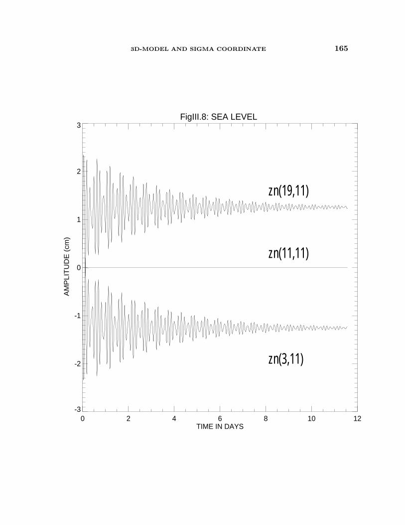
3D-MODEL AND SIGMA COORDINATE 165
FigIII.8: SEA LEVEL
0 2 4 6 8 10 12TIME IN DAYS
-3
-2
-1
0
1
2
3
AM
PLI
TU
DE
(cm
)
zn(19,11)
zn(11,11)
zn(3,11)
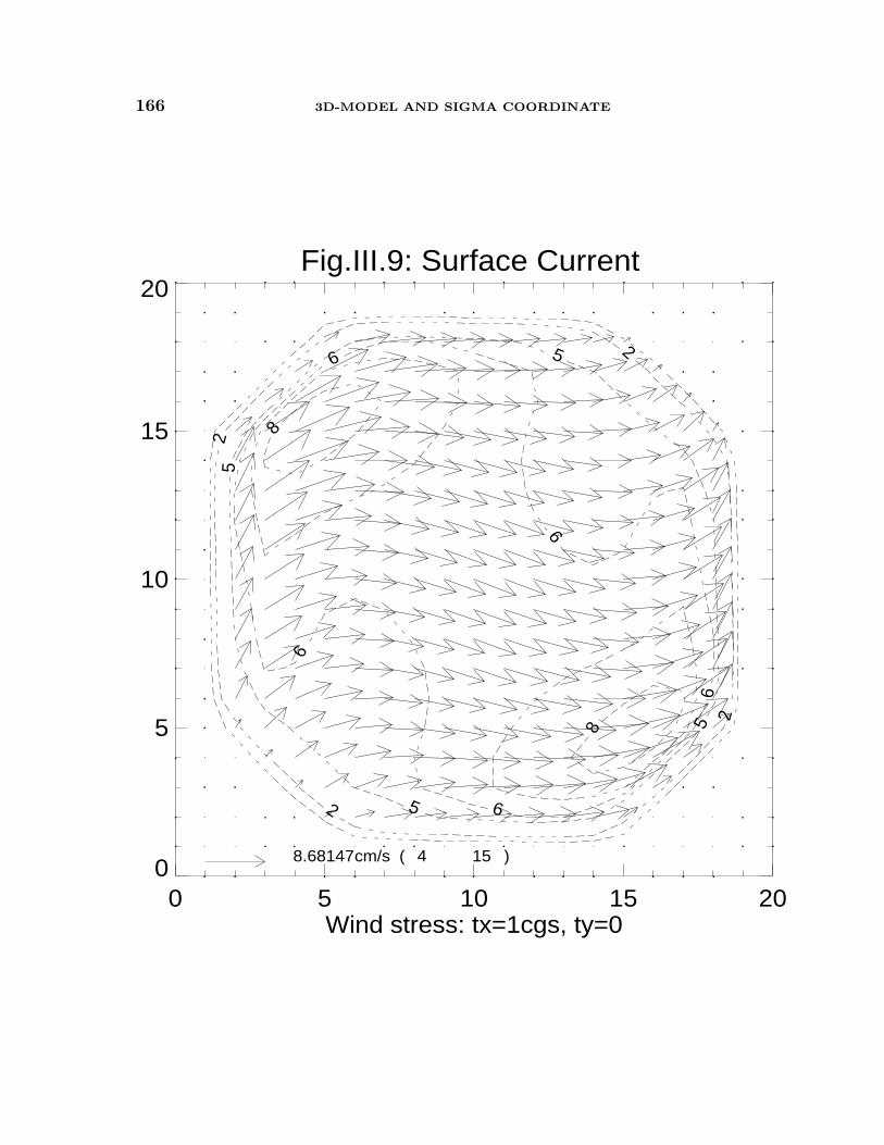
166 3D-MODEL AND SIGMA COORDINATE
Fig.III.9: Surface Current
0 5 10 15 20Wind stress: tx=1cgs, ty=0
0
5
10
15
20
2
2
2
2
5
5
5
5
6
6
6
6
6
8
8
8.68147cm/s ( 4 15 )
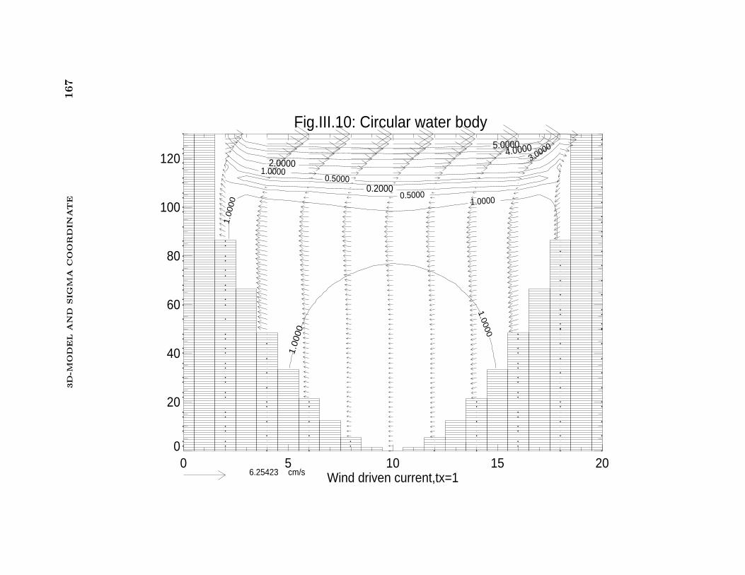
3D
-MO
DEL
AN
DSIG
MA
CO
OR
DIN
AT
E16
7
Fig.III.10: Circular water body
0 5 10 15 20Wind driven current,tx=1
0
20
40
60
80
100
120 3.00004.00005.0000
1.0000
1.00
00
1.0
000 1.00000.5000
0.20000.5000
1.00002.0000
6.25423 cm/s

168 3D-MODEL AND SIGMA COORDINATE
Problem No. 4, 3D- baroclinic model, sigma coordinate
In this problem the density stratification will be included. The density willcause additional gradients of pressure in the equations of motion. These gradientsalong the x and y directions can be expressed in σ coordinate as,
−gD2
ρ
∫ 0
σ
(∂ρ
∂x− Qx
D
∂ρ
∂σ)dσ = −gD2
ρ
∂
∂x
∫ 0
σ
ρdσ +gD
ρ
∂D
∂x
∫ 0
σ
σ∂ρ
∂σdσ
−gD2
ρ
∫ 0
σ
(∂ρ
∂y− Qy
D
∂ρ
∂σ)dσ = −gD2
ρ
∂
∂y
∫ 0
σ
ρdσ +gD
ρ
∂D
∂y
∫ 0
σ
σ∂ρ
∂σdσ
The full equations of motion now reads
∂
∂t(uD) +
∂
∂x(u2D) +
∂
∂y(uvD) +
∂
∂σ(Wu) − fDv
= −gD∂ζ
∂x+
1D
∂
∂σ(Nz
∂u
∂σ) + +Nh[
∂
∂xD
∂u
∂x+
∂
∂yD
∂u
∂y]
−gD2
ρ
∂
∂x
∫ 0
σ
ρdσ +gD
ρ
∂D
∂x
∫ 0
σ
σ∂ρ
∂σdσ (III.44)
∂
∂t(vD) +
∂
∂x(uvD) +
∂
∂y(v2D) +
∂
∂σ(Wv) + fDu
= −gD∂ζ
∂y+
1D
∂
∂σ(Nz
∂v
∂σ) + Nh[
∂
∂xD
∂v
∂x+
∂
∂yD
∂v
∂y]
−gD2
ρ
∂
∂y
∫ 0
σ
ρdσ +gD
ρ
∂D
∂y
∫ 0
σ
σ∂ρ
∂σdσ (III.45)
In the above equations the density distribution is assumed to be given eitherfrom observations or from calculations. Because density is function of salinity andtemperature one needs to introduce additional equations which express conservationof mass and heat. Therefore, to the above set of dependent variables the salinityand temperature ought to be added. Sea water density is calculated accordingly tothe formulas given by Friedrich, H. J and S. Levitus in J. Phys. Ocean., 2, 514-517, 1972. Salt and heat conservation equations are expressed as,
∂
∂t(DS) +
∂
∂x(uDS) +
∂
∂y(vDS) +
∂
∂σ(WS) =

3D-MODEL AND SIGMA COORDINATE 169
1D
∂
∂σ(Dz
∂S
∂σ) + Dh
∂
∂xD
∂S
∂x+ Dh
∂
∂yD
∂S
∂y(III.46)
∂
∂t(Dθ) +
∂
∂x(uDθ) +
∂
∂y(vDθ) +
∂
∂σ(Wθ) =
1D
∂
∂σ(Dz
∂θ
∂σ) + Dh
∂
∂xD
∂θ
∂x+ Dh
∂
∂yD
∂θ
∂y(III.47)
It is evident from these equations that they are closely related to equations ofmotion. Advective and convective terms in conservation equation are governed byvelocity components that are calculated through equations of motion, on the otherhand salinity and temperature define the density distribution and the baroclinicpressure which, in turn, drives currents. Calculations of salinity and currents, musttherefore, proceed in the same time loop. We start by constructing numerical formfor pressure terms in equations of motion. Consider term
∫ 0
σ
ρdσ
which occurs along both x and y directions, and if σ will be changed to z, theexpression is similar to the term defined on page 224 of NM. From the free surfaceto the first pressure point, the distance is 0.5 ∗hz1 and the pressure at the first gridpoint benith the free surface is prhj,k,1 = 0.5 ∗ hz1 ∗ ρj,k,1. The above integral can,therefore, be defined as a sum along the vertical direction by calculating pressureat any depth as
prhj,k,l = prhj,k,l−1 + 0.5 ∗ (hzl−1 ∗ ρj,k,l−1 + hzl ∗ ρj,k,l) (III.48)
Moreover, the pressure is defined in the pressure (salinity, temperature) points whichare located between velocity grid points, therefore it is easy to take derivatives alongx and y directions for the u and v components in the equations of motion.
The second pressure term is more complicated, it is resulted from coordinate’stransformation,
∫ 0
σ
σ∂ρ
∂σdσ
It can be changed to ∫ 0
σ
σdρ
as long as one remembers to take differences along the vertical (σ) direction. La-beling this pressure as prs, its value in the first point at the distance 0.5 ∗hz1 fromthe free surface can be assumed as zero. (If it is not zero, it can be estimated by
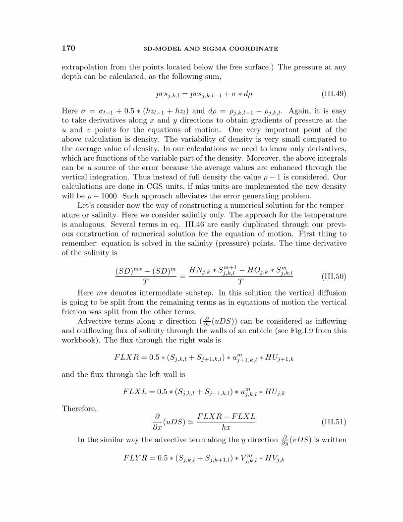
170 3D-MODEL AND SIGMA COORDINATE
extrapolation from the points located below the free surface.) The pressure at anydepth can be calculated, as the following sum,
prsj,k,l = prsj,k,l−1 + σ ∗ dρ (III.49)
Here σ = σl−1 + 0.5 ∗ (hzl−1 + hzl) and dρ = ρj,k,l−1 − ρj,k,l. Again, it is easyto take derivatives along x and y directions to obtain gradients of pressure at theu and v points for the equations of motion. One very important point of theabove calculation is density. The variability of density is very small compared tothe average value of density. In our calculations we need to know only derivatives,which are functions of the variable part of the density. Moreover, the above integralscan be a source of the error because the average values are enhanced through thevertical integration. Thus instead of full density the value ρ− 1 is considered. Ourcalculations are done in CGS units, if mks units are implemented the new densitywill be ρ− 1000. Such approach alleviates the error generating problem.
Let’s consider now the way of constructing a numerical solution for the temper-ature or salinity. Here we consider salinity only. The approach for the temperatureis analogous. Several terms in eq. III.46 are easily duplicated through our previ-ous construction of numerical solution for the equation of motion. First thing toremember: equation is solved in the salinity (pressure) points. The time derivativeof the salinity is
(SD)m∗ − (SD)m
T=
HNj,k ∗ Sm+1j,k,l −HOj,k ∗ Sm
j,k,l
T(III.50)
Here m∗ denotes intermediate substep. In this solution the vertical diffusionis going to be split from the remaining terms as in equations of motion the verticalfriction was split from the other terms.
Advective terms along x direction ( ∂∂x (uDS)) can be considered as inflowing
and outflowing flux of salinity through the walls of an cubicle (see Fig.I.9 from thisworkbook). The flux through the right wals is
FLXR = 0.5 ∗ (Sj,k,l + Sj+1,k,l) ∗ umj+1,k,l ∗HUj+1,k
and the flux through the left wall is
FLXL = 0.5 ∗ (Sj,k,l + Sj−1,k,l) ∗ umj,k,l ∗HUj,k
Therefore,∂
∂x(uDS) � FLXR− FLXL
hx(III.51)
In the similar way the advective term along the y direction ∂∂y (vDS) is written
FLY R = 0.5 ∗ (Sj,k,l + Sj,k+1,l) ∗ V mj,k,l ∗HVj,k
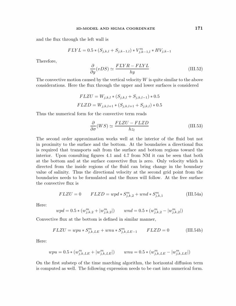
3D-MODEL AND SIGMA COORDINATE 171
and the flux through the left wall is
FLY L = 0.5 ∗ (Sj,k,l + Sj,k−1,l) ∗ V mj,k−1,l ∗HVj,k−1
Therefore,∂
∂y(vDS) � FLY R− FLY L
hy(III.52)
The convective motion caused by the vertical velocity W is quite similar to the aboveconsiderations. Here the flux through the upper and lower surfaces is considered
FLZU = Wj,k,l ∗ (Sj,k,l + Sj,k,l−1) ∗ 0.5
FLZD = Wj,k,l+1 ∗ (Sj,k,l+1 + Sj,k,l) ∗ 0.5
Thus the numerical form for the convective term reads
∂
∂σ(WS) � FLZU − FLZD
hzl(III.53)
The second order approximation works well at the interior of the fluid but notin proximity to the surface and the bottom. At the boundaries a directional fluxis required that transports salt from the surface and bottom regions toward theinterior. Upon consulting figures 4.1 and 4.7 from NM it can be seen that bothat the bottom and at the surface convective flux is zero. Only velocity which isdirected from the inside regions of the fluid can bring change in the boundaryvalue of salinity. Thus the directional velocity at the second grid point from theboundaries needs to be formulated and the fluxes will follow. At the free surfacethe convective flux is
FLZU = 0 FLZD = wpd ∗ Smj,k,2 + wnd ∗ Sm
j,k,1 (III.54a)
Here:wpd = 0.5 ∗ (wm
j,k,2 + |wmj,k,2|) wnd = 0.5 ∗ (wm
j,k,2 − |wmj,k,2|)
Convective flux at the bottom is defined in similar manner,
FLZU = wpu ∗ Smj,k,LE + wnu ∗ Sm
j,k,LE−1 FLZD = 0 (III.54b)
Here:
wpu = 0.5 ∗ (wmj,k,LE + |wm
j,k,LE|) wnu = 0.5 ∗ (wmj,k,LE − |wm
j,k,LE|)
On the first substep of the time marching algorithm, the horizontal diffusion termis computed as well. The following expression needs to be cast into numerical form.
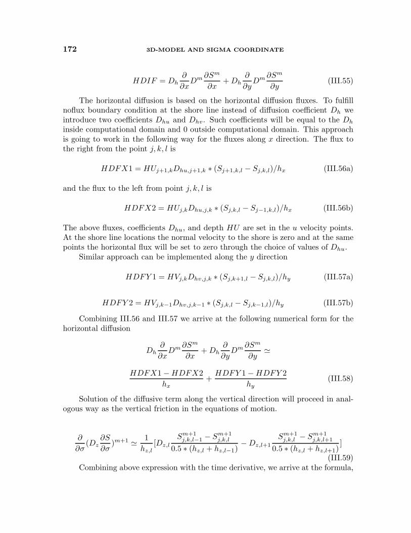
172 3D-MODEL AND SIGMA COORDINATE
HDIF = Dh∂
∂xDm ∂Sm
∂x+ Dh
∂
∂yDm ∂Sm
∂y(III.55)
The horizontal diffusion is based on the horizontal diffusion fluxes. To fulfillnoflux boundary condition at the shore line instead of diffusion coefficient Dh weintroduce two coefficients Dhu and Dhv. Such coefficients will be equal to the Dh
inside computational domain and 0 outside computational domain. This approachis going to work in the following way for the fluxes along x direction. The flux tothe right from the point j, k, l is
HDFX1 = HUj+1,kDhu,j+1,k ∗ (Sj+1,k,l − Sj,k,l)/hx (III.56a)
and the flux to the left from point j, k, l is
HDFX2 = HUj,kDhu,j,k ∗ (Sj,k,l − Sj−1,k,l)/hx (III.56b)
The above fluxes, coefficients Dhu, and depth HU are set in the u velocity points.At the shore line locations the normal velocity to the shore is zero and at the samepoints the horizontal flux will be set to zero through the choice of values of Dhu.
Similar approach can be implemented along the y direction
HDFY 1 = HVj,kDhv,j,k ∗ (Sj,k+1,l − Sj,k,l)/hy (III.57a)
HDFY 2 = HVj,k−1Dhv,j,k−1 ∗ (Sj,k,l − Sj,k−1,l)/hy (III.57b)
Combining III.56 and III.57 we arrive at the following numerical form for thehorizontal diffusion
Dh∂
∂xDm ∂Sm
∂x+ Dh
∂
∂yDm ∂Sm
∂y�
HDFX1 −HDFX2hx
+HDFY 1 −HDFY 2
hy(III.58)
Solution of the diffusive term along the vertical direction will proceed in anal-ogous way as the vertical friction in the equations of motion.
∂
∂σ(Dz
∂S
∂σ)m+1 � 1
hz,l[Dz,l
Sm+1j,k,l−1 − Sm+1
j,k,l
0.5 ∗ (hz,l + hz,l−1)−Dz,l+1
Sm+1j,k,l − Sm+1
j,k,l+1
0.5 ∗ (hz,l + hz,l+1)]
(III.59)Combining above expression with the time derivative, we arrive at the formula,
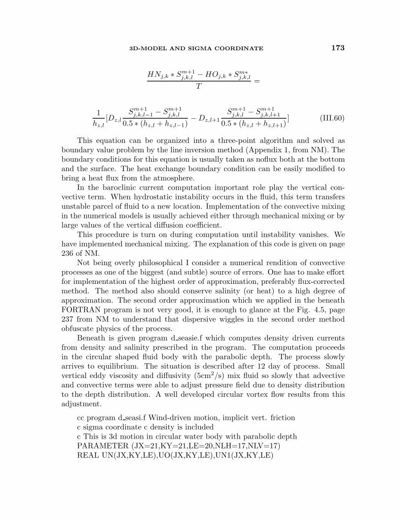
3D-MODEL AND SIGMA COORDINATE 173
HNj,k ∗ Sm+1j,k,l −HOj,k ∗ Sm∗
j,k,l
T=
1hz,l
[Dz,l
Sm+1j,k,l−1 − Sm+1
j,k,l
0.5 ∗ (hz,l + hz,l−1)−Dz,l+1
Sm+1j,k,l − Sm+1
j,k,l+1
0.5 ∗ (hz,l + hz,l+1)] (III.60)
This equation can be organized into a three-point algorithm and solved asboundary value problem by the line inversion method (Appendix 1, from NM). Theboundary conditions for this equation is usually taken as noflux both at the bottomand the surface. The heat exchange boundary condition can be easily modified tobring a heat flux from the atmosphere.
In the baroclinic current computation important role play the vertical con-vective term. When hydrostatic instability occurs in the fluid, this term transfersunstable parcel of fluid to a new location. Implementation of the convective mixingin the numerical models is usually achieved either through mechanical mixing or bylarge values of the vertical diffusion coefficient.
This procedure is turn on during computation until instability vanishes. Wehave implemented mechanical mixing. The explanation of this code is given on page236 of NM.
Not being overly philosophical I consider a numerical rendition of convectiveprocesses as one of the biggest (and subtle) source of errors. One has to make effortfor implementation of the highest order of approximation, preferably flux-correctedmethod. The method also should conserve salinity (or heat) to a high degree ofapproximation. The second order approximation which we applied in the beneathFORTRAN program is not very good, it is enough to glance at the Fig. 4.5, page237 from NM to understand that dispersive wiggles in the second order methodobfuscate physics of the process.
Beneath is given program d seasie.f which computes density driven currentsfrom density and salinity prescribed in the program. The computation proceedsin the circular shaped fluid body with the parabolic depth. The process slowlyarrives to equilibrium. The situation is described after 12 day of process. Smallvertical eddy viscosity and diffusivity (5cm2/s) mix fluid so slowly that advectiveand convective terms were able to adjust pressure field due to density distributionto the depth distribution. A well developed circular vortex flow results from thisadjustment.
cc program d seasi.f Wind-driven motion, implicit vert. frictionc sigma coordinate c density is includedc This is 3d motion in circular water body with parabolic depthPARAMETER (JX=21,KY=21,LE=20,NLH=17,NLV=17)REAL UN(JX,KY,LE),UO(JX,KY,LE),UN1(JX,KY,LE)
174 3D-MODEL AND SIGMA COORDINATE
REAL ZN(JX,KY),ZO(JX,KY),H(JX,ky),ENU(JX,KY,LE)REAL HZ(LE),TAUSX(JX,KY),TAUBX(JX,KY),UA(JX,KY)REAL W(JX,KY,LE+1),hu(jx,ky),upX(jx,le),wpX(jx,le)REAL upY(KY,le),wpY(KY,le),upxx(JX,KY,LE),UPYY(JX,KY,LE)real uai(jx,KY),HUN(JX,ky),HN(JX,ky)REAL VAI(JX,KY),VO(JX,KY,LE),VN(JX,KY,LE),ENV(JX,KY,LE)REAL DV(JX,ky,LE),TAUSY(JX,KY),SN(JX,KY,LE)REAL TAUBY(JX,KY),HO(JX,KY),VA(JX,KY),hv(jx,ky),hvn(jx,ky)REAL VN1(JX,KY,LE),WZ(JX,KY,LE+1),STV(JX,KY,LE)REAL DHU(JX,KY),DHV(JX,KY),SO(JX,KY,LE),ST(JX,KY,LE)REAL RHO(JX,KY,LE),PRH(JX,KY,LE),PRS(JX,KY,LE)REAL TO(JX,KY,LE),TT(JX,KY,LE),TN(JX,KY,LE),TTV(JX,KY,LE)real a(le+1),b(LE+1),c(LE+1),EN(JX,KY,LE)real d(LE+1),e(LE+1),s(LE+1)REAL ALP(7)/-7.2169E-2,4.9762E-2,8.056E-1,-7.5911E-3,1-3.0063E-3,3.5187E-5,3.7297E-5/integer js(nlh),je(nlh),ks(nlh),ke(nlh)integer jsv(nlv),jev(nlv),ksv(nlv),kev(nlv)open (unit=4,file=’parab.dat’,status=’unknown’)open (unit=3,file=’parab.ind’,status=’unknown’)open (unit=9,file=’wpy.dat’,status=’unknown’)open (unit=10,file=’z.dat’,status=’unknown’)open (unit=11,file=’momaxz1.dat’,status=’unknown’)open (unit=12,file=’eni.dat’,status=’unknown’)open (unit=15,file=’wpx.dat’,status=’unknown’)open (unit=16,file=’upx.dat’,status=’unknown’)open (unit=17,file=’upy.dat’,status=’unknown’)open (unit=20,file=’depthx.dat’,status=’unknown’)open (unit=21,file=’depthy.dat’,status=’unknown’)open (unit=7,file=’UPXX.dat’,status=’unknown’)open (unit=8,file=’UPYY.dat’,status=’unknown’)open (unit=18,file=’s.dat’,status=’unknown’)open (unit=19,file=’s1.dat’,status=’unknown’)open (unit=22,file=’t.dat’,status=’unknown’)open (unit=23,file=’t1.dat’,status=’unknown’)open (unit=24,file=’rho.dat’,status=’unknown’)open (unit=25,file=’rho1.dat’,status=’unknown’)read(4,*)((h(j,k),j=1,JX),k=1,ky)do j=1,jxdo K=1,KYIF(H(J,K).LT.500.)H(J,K)=500.hn(j,k)=h(j,k)

3D-MODEL AND SIGMA COORDINATE 175
ho(j,k)=h(j,k)END DOEND DOc Index : horizontal line, verticalc write (6,101) nlhc 101 format(4i6)do i=1,nlhread (3,100) ks(i),ke(i),js(i),je(i)100 format(4i4)enddocc write (6,101) nlvdo i=1,nlvread (3,100) jsv(i),jev(i),ksv(i),kev(i)enddocclose (3)write(20,*)(h(j,11),j=1,jx)write(21,*)(h(11,k),k=1,ky)C PRINT*,(ALP(I),I=1,7)DO K=1,KYHU(1,K)=HO(1,K)HUN(1,K)=HN(1,K)end dodo j=2,jxdo k=1,kyHU(j,k)=0.5*(Ho(j-1,k)+ho(j,k))HUN(j,k)=0.5*(Hn(j-1,k)+hn(j,k))end doend dodo j=1,JXHV(J,KY)=Ho(J,KY)HVN(J,KY)=Hn(J,KY)END DODO J=1,JXDO K=1,KY-1HV(J,K)=0.5*(HO(J,K)+HO(J,K+1))HVN(J,K)=0.5*(HN(J,K)+HN(J,K+1))end doend doDO J=1,JXDO K=1,KY

176 3D-MODEL AND SIGMA COORDINATE
ua(j,K)=0.va(j,k)=0.zo(j,K)=0.zn(j,k)=0.DHU(J,K)=0.DHV(J,K)=0.end doEND DOdo j=1,jxDO K=1,KYdo l=1,leun(j,K,l)=0.un1(j,k,l)=0.uo(j,K,l)=0.vn(J,K,L)=0.VO(J,K,L)=0.VN1(J,K,L)=0.w(j,k,l)=0.wZ(j,k,l)=0.ENU(J,K,L)=0.ENV(J,K,L)=0.SO(J,K,L)=0.ST(J,K,L)=0.STV(J,K,L)=0.SN(J,K,L)=0.PRS(J,K,L)=0.PRH(J,K,L)=0.RHO(J,K,L)=0.TO(J,K,L)=0.TT(J,K,L)=0.TTV(J,K,L)=0.TN(J,K,L)=0.end doend doEND DOc INITIAL SALINITYc THE STUFF BELOW IS FOR INITIAL SALINITYC AND TEMPERATURE IT CAN BE USED FOR PLOTTING THROUGHC PROGRAM PREPARE SAL.Fdo j=1,jxDO K=1,KYdo l=1,le

3D-MODEL AND SIGMA COORDINATE 177
SO(J,K,L)=FLOAT(L)*0.345+19.655+2.5*float(j)/float(jx)2+2.5*float(K)/float(KY)TO(J,K,L)=15.+1.*FLOAT(LE)/(5.*FLOAT(L))+2.*float(j)/float(jx)*+2.*float(K)/float(KY)end doend doEND DODO L=1,LEwrite(19,*)(so(j,11,L),j=1,jx)write(23,*)(TO(j,11,L),j=1,jx)END DOC GO TO 222C SET variable SPACE STEP ALONG VERTICAL DIRECTIONDO L=1,leHZ(L)=0.05END DOC ALL COEFFICIENTSc==================================c Time stepT = 100.FC=1.458E-4G=981.c SPACE STEPS ALONG X AND YHX=10.E5HY=10.E5RF1=2.6E-3RF2=2.6E-3c HORIZONTAL EDDY VISCOSITYAH=1.0e7c HORIZONTAL EDDY DIFFUSIVITY ALONG X DIRECTIONdo n=1,nlhdo j=js(n)+1,je(n)do k=ks(n),ke(n)DHU(J,K)=(1.0e7)*T/(HX*HX)END DOEND DOend dodo m=1,nlvcdo j=jsv(m),jev(m)do k=ksv(m),kev(m)-1DHV(J,K)=(1.0e7)*T/(HY*HY)
178 3D-MODEL AND SIGMA COORDINATE
END DOEND DOend doC COMBINATIONAL PARAMETERSTRF=T*RF1PL=T/HXGPL=G*PLPLL=AH*T/(HX*HX)PF=T/HYGPF=G*PFPFF=AH*T/(HY*HY)TFC=T*FCTWHX=2.*hx ! for vertical velocityTWHY=2.*hY ! for vertical velocityC START TIME LOOP INDEX N RUNS UNTIL N=MONc************************************c MON=86400mon=10000c mon=10nn=0C8888888888888888888888888888888888888850 Nn=Nn+1C SOME COEFFICIENTS ARE VARIABLEC SET WIND FOR INITIAL EXPERIMENTDO J=1,JXDO K=1,KYTAUSX(J,K)=0.TAUSY(J,K)=0.END DOEND DOC DO NOT INTRODUCE STRONG WIND UBRUPTLYc if (n.lt.1000)thenc DO J=1,JXc DO K=1,KYc TAUSX(J,K)=float(nN)/1000.c TAUSY(J,K)=0.c END DOc END DOc end ifC EDDY VISCOSITY IS CONSTANTDO 33J=1,JXdo 33 k=1,ky
3D-MODEL AND SIGMA COORDINATE 179
DO 33 L=1,LeEN(J,k,L)=5.33 CONTINUEDO J=1,JXdo k=1,kyDO L=1,LEENU(J,k,L)=0.5*(EN(J,K,L)+EN(J,K-1,L))ENV(J,K,L)=0.5*(EN(J,K,L)+EN(J+1,K,L))DV(J,K,L)=5.END DOEND DOEND DOc IN SPACE COEFFICIENT OF EDDY VISCOSITY SHOULD BEC LOCATED IN Z (OR PRESSURE) POINTSC COMPUTATION OF U VELOCITY, closed boundary, velocity is zero atC J=1 AND J=JX.c - + + - + - +c 1 jx jx+1c left rightC VELOCITY IN THE AIRC go to 225DO 499 n=1,nlhdo 499j=js(n)+1,je(n)do 499k=ks(n),ke(n)UAI(J,K)=UO(J,K,1)+HZ(1)*hu(j,K)*TAUSX(J,K)/ENU(J,K,1)499 continueDO 4 n=1,nlhdo 4 j=js(n)+1,je(n)do 4 k=ks(n),ke(n)C THIS GOES INTO HORIZONTAL FRICTIONDHU1=0.5*(HU(J,K)+HU(J,K+1))DHU2=0.5*(HU(J,K)+HU(J,K-1))C PRESSURE DUE TO DENSITYDPRH=HU(J,K)*HU(J,K)*GPL*(PRH(J,K,1)-PRH(J-1,K,1))PRSS=0.5*(PRS(J,K,1)+PRS(J-1,K,1))DPRS=GPL*HU(J,K)*(H(J,K)-H(J-1,K))*PRSSC SURFACE CONDITIONC CORIOLISVR=0.5*(VO(J,K,1)+VO(J,K-1,1))VL=0.5*(VO(J-1,K,1)+VO(J-1,K-1,1))UAV=0.5*(HO(J,K)*VR+HO(J-1,K)*VL)DSL=ZO(J,K)-ZO(J-1,K)
180 3D-MODEL AND SIGMA COORDINATE
DSLX=DSL*GPL*HU(J,K)HZP=0.5*(HZ(1)+HZ(2))*hu(j,K)DSU=(UO(J,K,1)-UO(J,K,2))/HZPc VFRS=(TAUSX(J,K)-ENU(J,K,2)*DSU)/HZ(1)C HORIZONTAL FRICTIONHFRUX=PLL*(UO(J+1,K,1)*H(J,K)+UO(J-1,K,1)*H(J-1,K)2-(H(J,K)+H(J-1,K))*UO(J,K,1))HFRUY=PFF*(UO(J,K+1,1)*DHU1+UO(J,K-1,1)*DHU23-(DHU1+DHU2)*UO(J,K,1))HFR=HFRUX+HFRUYC EVEN BETTER IMPROVED NONLINEAR TERMXc uwUSN=0.5*(UAI(J,K)+UO(J,K,1))USP=(UO(J,K,1)*HZ(2)+UO(J,K,2)*HZ(1))/(HZ(1)+HZ(2))waxn=0.5*(W(J-1,K,1)+W(J,K,1))WAXP=0.5*(W(J-1,K,2)+W(J,K,2))UW=T*(WAXN*USN-WAXP*USP)/HZ(1)C EVEN BETTER IMPROVED NONLINEAR TERMXc uv uuUAF=0.5*(UO(J,K,1)+UO(J+1,K,1))UAB=0.5*(UO(J,K,1)+UO(J-1,K,1))ONXF=0.5*(UO(J,K,1)*HU(J,K)+UO(J+1,K,1)*HU(J+1,K))ONXB=0.5*(UO(J,K,1)*HU(J,K)+UO(J-1,K,1)*HU(J-1,K))SUMNONX=PL*(ONXF*UAF-ONXB*UAB)C UVUAU=0.5*(UO(J,K,1)+UO(J,K+1,1))UAD=0.5*(UO(J,K-1,1)+UO(J,K,1))ONYU=0.5*(VO(J,K,1)*HV(J,K)+VO(J-1,K,1)*HV(J-1,K))ONYD=0.5*(VO(J,K-1,1)*HV(J,K-1)+VO(J-1,K-1,1)*HV(J-1,K-1))SUMNONY=PF*(UAU*ONYU-UAD*ONYD)SUMNON=SUMNONX+SUMNONY+UWUN1(J,K,1)=UO(J,K,1)*HU(J,K)-DSLX+TFC*UAV+HFR-SUMNON2-DPRH+DPRSUN1(J,K,1)=UN1(J,K,1)/HUN(J,K)LMM=LEDO 5 L=2,LMM-1C PRESSURE DUE TO DENSITYDPRH=HU(J,K)*HU(J,K)*GPL*(PRH(J,K,L)-PRH(J-1,K,L))PRSS=0.5*(PRS(J,K,L)+PRS(J-1,K,L))DPRS=GPL*HU(J,K)*(H(J,K)-H(J-1,K))*PRSSHZP=0.5*(HZ(L)+HZ(L+1))*HU(J,K)HZN=0.5*(HZ(L)+HZ(L-1))*HU(J,K)

3D-MODEL AND SIGMA COORDINATE 181
DSUN=(UO(J,K,L-1)-UO(J,K,L))/HZNDSUP=(UO(J,K,L)-UO(J,K,L+1))/HZPc VFR=(ENU(J,K,L)*DSUN-ENU(J,K,L+1)*DSUP)/HZ(L)C HORIZONTAL FRICTIONHFRUX=PLL*(UO(J+1,K,L)*H(J,K)+UO(J-1,K,L)*H(J-1,K)2-UO(J,K,L)*(H(J,K)+H(J-1,K)))HFRUY=PFF*(UO(J,K+1,L)*DHU1+UO(J,K-1,L)*DHU23-(DHU1+DHU2)*UO(J,K,L))HFR=HFRUX+HFRUYC CORIOLISVR=0.5*(VO(J,K,L)+VO(J,K-1,L))VL=0.5*(VO(J-1,K,L)+VO(J-1,K-1,L))UAV=0.5*(HO(J,K)*VR+HO(J-1,K)*VL)C EVEN BETTER IMPROVED NONLINEAR TERMXUAF=0.5*(UO(J,K,L)+UO(J+1,K,L))UAB=0.5*(UO(J,K,L)+UO(J-1,K,L))ONXF=0.5*(UO(J,K,L)*HU(J,K)+UO(J+1,K,L)*HU(J+1,K))ONXB=0.5*(UO(J,K,L)*HU(J,K)+UO(J-1,K,L)*HU(J-1,K))SUMNONX=PL*(ONXF*UAF-ONXB*UAB)C UVUAU=0.5*(UO(J,K,L)+UO(J,K+1,L))UAD=0.5*(UO(J,K-1,L)+UO(J,K,L))ONYU=0.5*(VO(J,K,L)*HV(J,K)+VO(J-1,K,L)*HV(J-1,K))ONYD=0.5*(VO(J,K-1,L)*HV(J,K-1)+VO(J-1,K-1,L)*HV(J-1,K-1))SUMNONY=PF*(UAU*ONYU-UAD*ONYD)SUMNON=SUMNONX+SUMNONYc vert deriv.waxn=0.5*(W(J-1,K,L)+W(J,K,L))WAXP=0.5*(W(J-1,K,L+1)+W(J,K,L+1))USN=(UO(J,K,L-1)*HZ(L)+UO(J,K,L)*HZ(L-1))/(HZ(L)+HZ(L-1))USP=(UO(J,K,L)*HZ(L+1)+UO(J,K,L+1)*HZ(L))/(HZ(L)+HZ(L+1))UW=T*(WAXN*USN-WAXP*USP)/HZ(L)SUMNON=SUMNON+UWUN1(J,K,L)=UO(J,K,L)*HU(J,K)-DSLX+TFC*UAV+HFR-SUMNON2-DPRH+DPRSUN1(J,K,L)=UN1(J,K,L)/HUN(J,K)5 CONTINUEC BOTTOM CONDITIONC PRESSURE DUE TO DENSITYDPRH=HU(J,K)*HU(J,K)*GPL*(PRH(J,K,LMM)-PRH(J-1,K,LMM))PRSS=0.5*(PRS(J,K,LMM)+PRS(J-1,K,LMM))DPRS=GPL*HU(J,K)*(H(J,K)-H(J-1,K))*PRSS
182 3D-MODEL AND SIGMA COORDINATE
C CORIOLISVR=0.5*(Vo(J,K,LMM)+Vo(J,K-1,LMM))VL=0.5*(Vo(J-1,K,LMM)+Vo(J-1,K-1,LMM))UAV=0.5*(HO(J,K)*VR+HO(J-1,K)*VL)c UAV1=0.5*(VR+VL)HZP=HZ(LMM)*HU(J,K)HZN=0.5*(HZ(LMM)+HZ(LMM-1))*HU(J,K)DSUP=2.*UO(J,K,LMM)/HZPDSUN=(UO(J,K,LMM-1)-UO(J,K,LMM))/HZNC HORIZONTAL FRICTIONHFRUX=PLL*(UO(J+1,K,LMM)*H(J,K)+UO(J-1,K,LMM)*H(J-1,K)2-UO(J,K,LMM)*(H(J,K)+H(J-1,K)))HFRUY=PFF*(UO(J,K+1,LMM)*DHU1+UO(J,K-1,LMM)*DHU23-(DHU1+DHU2)*UO(J,K,LMM))HFR=HFRUX+HFRUYC EVEN BETTER IMPROVED NONLINEAR TERMXUAF=0.5*(UO(J,K,LMM)+UO(J+1,K,LMM))UAB=0.5*(UO(J,K,LMM)+UO(J-1,K,LMM))ONXF=0.5*(UO(J,K,LMM)*HU(J,K)+UO(J+1,K,LMM)*HU(J+1,K))ONXB=0.5*(UO(J,K,LMM)*HU(J,K)+UO(J-1,K,LMM)*HU(J-1,K))SUMNONX=PL*(ONXF*UAF-ONXB*UAB)C UVUAU=0.5*(Uo(J,K,LMM)+Uo(J,K+1,LMM))UAD=0.5*(Uo(J,K-1,LMM)+Uo(J,K,LMM))ONYU=0.5*(Vo(J,K,LMM)*HV(J,K)+Vo(J-1,K,LMM)*HV(J-1,K))ONYD=0.5*(Vo(J,K-1,LMM)*HV(J,K-1)+2Vo(J-1,K-1,LMM)*HV(J-1,K-1))SUMNONY=PF*(UAU*ONYU-UAD*ONYD)SUMNON=SUMNONX+SUMNONYc vert deriv.HZMM=HZ(LMM)+HZ(LMM-1)waxn=0.5*(W(J-1,K,LMM)+W(J,K,LMM))WAXP=0.USN=(UO(J,K,L-1)*HZ(LMM)+UO(J,K,L)*HZ(LMM-1))/HZMMUSP=0.UW=T*(WAXN*USN-WAXP*USP)/HZ(LMM)SUMNON=SUMNON+UWUN1(J,K,LMM)=UO(J,K,LMM)*HU(J,K)-DSLX+TFC*UAV+HFR-
SUMNON2-DPRH+DPRSUN1(J,K,LMM)=UN1(J,K,LMM)/HUN(J,K)C UN(J,LMM)=0.

3D-MODEL AND SIGMA COORDINATE 183
4 CONTINUec VERTICAL FRICTION SPLIT FROM THE RESTDO 46 n=1,nlhdo 46 j=js(n)+1,je(n)do 46 k=ks(n),ke(n)TAUSX(J,k)=0.VR=0.5*(Vo(J,K,LE)+Vo(J,K-1,LE))VL=0.5*(Vo(J-1,K,LE)+Vo(J-1,K-1,LE))UAV1=0.5*(VR+VL)HZPP=HZ(LE)*HUn(J,K)C LOG OR NOT TO LOGCD=2.5*ALOG(1.25*HZPP)CD=1./(CD*CD)RF1=AMAX1(CD,RF2)PIERW=SQRT(UO(J,K,Le)*UO(J,K,Le)+uav1*uav1)TAUBX(J,k)=RF1*PIERW*UO(J,K,Le)HZP=0.5*(HZ(1)+HZ(2))*hu(j,k)C(1)=T*ENU(J,K,2)/(HZ(1)*huN(j,k)*HZP)D(1)=UN1(J,K,1)DO L=2,LE-1HZP=0.5*(HZ(L)+HZ(L+1))*hu(j,k)HZN=0.5*(HZ(L)+HZ(L-1))*hu(j,k)A(L)=T*ENU(j,k,L)/(HZ(L)*huN(j,k)*HZN)C(L)=T*ENU(J,K,L+1)/(HZ(L)*huN(j,k)*HZP)B(L)=1+A(L)+C(L)D(L)=UN1(J,K,L)END DOHZN=0.5*(HZ(LE)+HZ(LE-1))*hu(j,k)HZP=0.5*(HZ(LE)+HZ(LE+1))*hu(j,k)D(LE)=UN1(J,K,LE)A(Le)=T*ENU(j,k,Le)/(HZ(Le)*huN(j,k)*Hzn)C(Le)=T*ENU(J,K,Le)/(HZ(Le)*huN(j,k)*HZP)B(Le)=1+A(Le)+C(Le)S(1)=C(1)/(1.+C(1))E(1)=UN1(J,K,1)+T*TAUSX(J,K)/(HZ(1)*huN(j,k))E(1)=E(1)/(1.+C(1))DO L=2,LE-1C VERTICAL FRICTION CONTINUEDENOM=B(L)-S(L-1)*A(L)S(L)=C(L)/DENOME(L)=(D(L)+A(L)*E(L-1))/DENOMEND DO
184 3D-MODEL AND SIGMA COORDINATE
A1=A(LE)*E(LE-1)+D(LE)-T*TAUBX(J,K)/(HZ(LE)*huN(j,k))A2=1.+A(le)*(1.-S(LE-1))UN(J,K,LE)=A1/A2DO L=LE-1,1,-1UN(J,K,L)=UN(J,K,L+1)*S(L)+E(L)END DO46 CONTINUEC COMPUTATION OF V VELOCITYC VELOCITY IN THE AIRdo 2001 m=1,nlvcdo 2001 j=jsv(m),jev(m)do 2001 k=ksv(m),kev(m)-1VAI(J,K)=VO(J,K,1)+HZ(1)*hV(j,K)*TAUSY(J,K)/ENV(J,K,1)2001 continuedo 6 m=1,nlvc if(ksv(m).eq.kev(m)) go to 6do 6 j=jsv(m),jev(m)do 6 k=ksv(m),kev(m)-1C THIS GOES INTO HORIZONTAL FRICTIONDHV1=0.5*(HV(J,K)+HV(J+1,K))DHV2=0.5*(HV(J,K)+HV(J-1,K))C PRESSURE DUE TO DENSITYDPRH=HU(J,K)*HU(J,K)*GPF*(PRH(J,K+1,1)-PRH(J,K,1))PRSS=0.5*(PRS(J,K,1)+PRS(J,K+1,1))DPRS=GPF*HU(J,K)*(H(J,K+1)-H(J,K))*PRSSC SURFACE CONDITIONDSL=ZO(J,K+1)-ZO(J,K)DSLY=GPF*DSL*HV(J,K)HZP=0.5*(HZ(1)+HZ(2))*HV(J,K)C CORIOLIS TERMUG=0.5*(UN(J,K+1,1)+UN(J+1,K+1,1))UD=0.5*(UN(J,K,1)+UN(J+1,K,1))VAUN=0.5*(HN(J,K+1)*UG+HN(J,K)*UD)DSV=(VO(J,K,1)-VO(J,K,2))/HZPC VFRS=(TAUSY(J,K)-ENV(J,K,2)*DSV)/HZ(1)C HORIZONTAL FRICTIONHFRVY=PFF*(VO(J,K+1,1)*H(J,K+1)+VO(J,K-1,1)*H(J,K)2-(H(J,K)+H(J,K+1))*VO(J,K,1))HFRVX=PLL*(VO(J+1,K,1)*DHV1+VO(J-1,K,1)*DHV23-(DHV1+DHV2)*VO(J,K,1))HFR=HFRVX+HFRVY

3D-MODEL AND SIGMA COORDINATE 185
C HFR=PLL*HV(J,K)*(VO(J+1,K,1)+VO(J-1,K,1)-2.*VO(J,K,1))+C 2PFF*HV(J,K)*(VO(J,K+1,1)+VO(J,K-1,1)-2.*VO(J,K,1))C EVEN BETTER NONLINEARC UVVALX=0.5*(VO(J,K,1)+VO(J-1,K,1))VARX=0.5*(VO(J,K,1)+VO(J+1,K,1))ONXL=0.5*(HU(J,K+1)*UO(J,K+1,1)+HU(J,K)*UO(J,K,1))ONXR=0.5*(HU(J+1,K+1)*UO(J+1,K+1,1)+HU(J+1,K)*UO(J+1,K,1))SUMNONX=PL*(ONXR*VARX-ONXL*VALX)C VVVAGY=0.5*(VO(J,K+1,1)+VO(J,K,1))VADY=0.5*(VO(J,K-1,1)+VO(J,K,1))ONYU=0.5*(HV(J,K+1)*VO(J,K+1,1)+HV(J,K)*VO(J,K,1))ONYD=0.5*(HV(J,K-1)*VO(J,K-1,1)+HV(J,K)*VO(J,K,1))SUMNONY=PF*(ONYU*VAGY-ONYD*VADY)SUMNON=SUMNONX+SUMNONYCWVVSU=0.5*(VO(J,K,1)+VAI(J,K))VSD=(VO(J,K,1)*HZ(2)+VO(J,K,2)*HZ(1))/(HZ(1)+HZ(2))WAG=0.5*(W(J,K,1)+W(J,K+1,1))WAD=0.5*(W(J,K,2)+W(J,K+1,2))WV=T*(VSU*WAG-VSD*WAD)/HZ(1)SUMNON=SUMNON+WVVN1(J,K,1)=VO(J,K,1)*HV(J,K)-TFC*VAUN-DSLY+HFR-2SUMNON-DPRH+DPRSVN1(J,K,1)=VN1(J,K,1)/HVN(J,K)DO L=2,LE-1C PRESSURE DUE TO DENSITYDPRH=HU(J,K)*HU(J,K)*GPF*(PRH(J,K+1,L)-PRH(J,K,L))PRSS=0.5*(PRS(J,K,L)+PRS(J,K+1,L))DPRS=GPF*HU(J,K)*(H(J,K+1)-H(J,K))*PRSSC CORIOLIS TERMUG=0.5*(UN(J,K+1,L)+UN(J+1,K+1,L))UD=0.5*(UN(J,K,L)+UN(J+1,K,L))VAUN=0.5*(HN(J,K+1)*UG+HN(J,K)*UD)HZP=0.5*(HZ(L)+HZ(L+1))*HV(J,K)HZN=0.5*(HZ(L)+HZ(L-1))*HV(J,K)DSVN=(VO(J,K,L-1)-VO(J,K,L))/HZNDSVP=(VO(J,K,L)-VO(J,K,L+1))/HZPC VFR=(ENV(J,K,L)*DSVN-ENV(J,K,L+1)*DSVP)/HZ(L)C HORIZONTAL FRICTIONC HFR=PLL*HV(J,K)*(VO(J+1,K,L)+VO(J-1,K,L)-2.*VO(J,K,L))+

186 3D-MODEL AND SIGMA COORDINATE
C 2PFF*HV(J,K)*(VO(J,K+1,L)+VO(J,K-1,L)-2.*VO(J,K,L))C HORIZONTAL FRICTIONHFRVY=PFF*(VO(J,K+1,L)*H(J,K+1)+VO(J,K-1,L)*H(J,K)2-(H(J,K)+H(J,K+1))*VO(J,K,L))HFRVX=PLL*(VO(J+1,K,L)*DHV1+VO(J-1,K,L)*DHV23-(DHV1+DHV2)*VO(J,K,L))HFR=HFRVX+HFRVYC EVEN BETTER NONLINEARC UVVALX=0.5*(VO(J,K,L)+VO(J-1,K,L))VARX=0.5*(VO(J,K,L)+VO(J+1,K,L))ONXL=0.5*(HU(J,K+1)*UO(J,K+1,L)+HU(J,K)*UO(J,K,L))ONXR=0.5*(HU(J+1,K+1)*UO(J+1,K+1,L)+HU(J+1,K)*UO(J+1,K,L))SUMNONX=PL*(ONXR*VARX-ONXL*VALX)C VVVAGY=0.5*(VO(J,K+1,L)+VO(J,K,L))VADY=0.5*(VO(J,K-1,L)+VO(J,K,L))ONYU=0.5*(HV(J,K+1)*VO(J,K+1,L)+HV(J,K)*VO(J,K,L))ONYD=0.5*(HV(J,K-1)*VO(J,K-1,L)+HV(J,K)*VO(J,K,L))SUMNONY=PF*(ONYU*VAGY-ONYD*VADY)SUMNON=SUMNONX+SUMNONYCWVVSU=(VO(J,K,L-1)*HZ(L)+VO(J,K,L)*HZ(L-1))/(HZ(L)+HZ(L-1))VSD=(VO(J,K,L)*HZ(L+1)+VO(J,K,L+1)*HZ(L))/(HZ(L)+HZ(L+1))WAG=0.5*(W(J,K,L)+W(J,K+1,L))WAD=0.5*(W(J,K,L+1)+W(J,K+1,L+1))WV=T*(VSU*WAG-VSD*WAD)/HZ(L)SUMNON=SUMNON+WVVN1(J,K,L)=VO(J,K,L)*HV(J,K)-TFC*VAUN-DSLY+HFR-2SUMNON-DPRH+DPRSVN1(J,K,L)=VN1(J,K,L)/HVN(J,K)end doC BOTTOMC PRESSURE DUE TO DENSITYDPRH=HU(J,K)*HU(J,K)*GPF*(PRH(J,K+1,LE)-PRH(J,K,LE))PRSS=0.5*(PRS(J,K,LE)+PRS(J,K+1,LE))DPRS=GPF*HU(J,K)*(H(J,K+1)-H(J,K))*PRSSC CORIOLIS TERMUG=0.5*(UN(J,K+1,LE)+UN(J+1,K+1,LE))UD=0.5*(UN(J,K,LE)+UN(J+1,K,LE))VAUN=0.5*(HN(J,K+1)*UG+HN(J,K)*UD)C VAU=0.25*(UO(J,K+1,LE)+UO(J+1,K+1,LE)+UO(J,K,LE)

3D-MODEL AND SIGMA COORDINATE 187
C 2+UO(J+1,K,LE))HZP=HZ(LE)*HV(J,K)HZN=0.5*(HZ(LE)+HZ(LE-1))*HV(J,K)DSVN=(VO(J,K,LE-1)-VO(J,K,LE))/HZNC HORIZONTAL FRICTIONHFRVY=PFF*(VO(J,K+1,LE)*H(J,K+1)+VO(J,K-1,LE)*H(J,K)2-(H(J,K)+H(J,K+1))*VO(J,K,LE))HFRVX=PLL*(VO(J+1,K,LE)*DHV1+VO(J-1,K,LE)*DHV23-(DHV1+DHV2)*VO(J,K,LE))HFR=HFRVX+HFRVYC HFR=PLL*HV(J,K)*(VO(J+1,K,LE)+VO(J-1,K,LE)-2.*VO(J,K,LE))+C 2PFF*HV(J,K)*(VO(J,K+1,LE)+VO(J,K-1,LE)-2.*VO(J,K,LE))C EVEN BETTER NONLINEARC UVVALX=0.5*(VO(J,K,LE)+VO(J-1,K,LE))VARX=0.5*(VO(J,K,LE)+VO(J+1,K,LE))ONXL=0.5*(HU(J,K+1)*UO(J,K+1,LE)+HU(J,K)*UO(J,K,LE))ONXR=0.5*(HU(J+1,K+1)*UO(J+1,K+1,LE)+HU(J+1,K)*UO(J+1,K,LE))SUMNONX=PL*(ONXR*VARX-ONXL*VALX)C VVVAGY=0.5*(VO(J,K+1,LE)+VO(J,K,LE))VADY=0.5*(VO(J,K-1,LE)+VO(J,K,LE))ONYU=0.5*(HV(J,K+1)*VO(J,K+1,LE)+HV(J,K)*VO(J,K,LE))ONYD=0.5*(HV(J,K-1)*VO(J,K-1,LE)+HV(J,K)*VO(J,K,LE))SUMNONY=PF*(ONYU*VAGY-ONYD*VADY)SUMNON=SUMNONX+SUMNONYCWVVSU=(VO(J,K,LE-1)*HZ(LE)+VO(J,K,LE)*HZ(LE-1))/2(HZ(LE)+HZ(LE-1))VSD=0.WAG=0.5*(W(J,K,LE)+W(J,K+1,LE))WAD=0.WV=T*(VSU*WAG-VSD*WAD)/HZ(LE)SUMNON=SUMNON+WVVN1(J,K,LE)=VO(J,K,LE)*HV(J,K)-TFC*VAUN-DSLY+HFR-2SUMNON-DPRH+DPRSVN1(J,K,LE)=VN1(J,K,LE)/HVN(J,K)6 continuec VERTICAL FRICTION SPLIT FROM THE RESTdo 7 m=1,nlvcdo 7 j=jsv(m),jev(m)

188 3D-MODEL AND SIGMA COORDINATE
do 7 k=ksv(m),kev(m)-1HZPP=HZ(LE)*HVn(J,K)VAU=0.25*(UO(J,K+1,LE)+UO(J+1,K+1,LE)+UO(J,K,LE)2+UO(J+1,K,LE))C LOG OR NOT TO LOGCD=2.5*ALOG(1.25*HZPP)CD=1./(CD*CD)RF1=AMAX1(CD,RF2)PIERW=SQRT(VO(J,K,Le)*VO(J,K,Le)+VAU*VAU)TAUBY(J,k)=RF1*PIERW*VO(J,K,Le)HZP=0.5*(HZ(1)+HZ(2))*hV(j,k)C(1)=T*ENV(J,K,2)/(HZ(1)*hVN(j,k)*HZP)D(1)=VN1(J,K,1)DO L=2,LE-1HZP=0.5*(HZ(L)+HZ(L+1))*hV(j,k)HZN=0.5*(HZ(L)+HZ(L-1))*hV(j,k)A(L)=T*ENV(j,k,L)/(HZ(L)*HVN(j,k)*HZN)C(L)=T*ENV(J,K,L+1)/(HZ(L)*HVN(j,k)*HZP)B(L)=1+A(L)+C(L)D(L)=VN1(J,K,L)END DOHZN=0.5*(HZ(LE)+HZ(LE-1))*HV(j,k)HZP=0.5*(HZ(LE)+HZ(LE+1))*HV(j,k)D(LE)=VN1(J,K,LE)A(Le)=T*ENV(j,k,Le)/(HZ(Le)*HVN(j,k)*Hzn)C(Le)=T*ENV(J,K,Le)/(HZ(Le)*HVN(j,k)*HZP)B(Le)=1+A(Le)+C(Le)S(1)=C(1)/(1.+C(1))E(1)=VN1(J,K,1)+T*TAUSX(J,K)/(HZ(1)*HVN(j,k))E(1)=E(1)/(1.+C(1))DO L=2,LE-1C VERTICAL FRICTION CONTINUEDENOM=B(L)-S(L-1)*A(L)S(L)=C(L)/DENOME(L)=(D(L)+A(L)*E(L-1))/DENOMEND DOA1=A(LE)*E(LE-1)+D(LE)-T*TAUBX(J,K)/(HZ(LE)*HVN(j,k))A2=1.+A(le)*(1.-S(LE-1))VN(J,K,LE)=A1/A2DO L=LE-1,1,-1VN(J,K,L)=VN(J,K,L+1)*S(L)+E(L)END DO
3D-MODEL AND SIGMA COORDINATE 189
7 CONTINUEC SEA LEVELC FIRST AVERAGE VELOCITY ALONG VERTICAL DIRECTIONc print *, un(2,5,1),un(3,5,1)DO 9 n=1,nlhdo 9 j=js(n)+1,je(n)do 9 k=ks(n),ke(n)MM=LEC+++++++++++++++++++++++++++++++++++++++UA(J,k)=0.DO 10 L=MM,1,-1UA(J,K)=UA(J,K)+UN(J,K,L)*HZ(L)10 CONTINUE9 CONTINUEc***************************************do 2000 m=1,nlvif(ksv(m).eq.kev(m)) go to 2000cdo 2000 j=jsv(m),jev(m)do 2000 k=ksv(m),kev(m)-1MM=LEVA(J,K)=0.DO 12 L=MM,1,-1VA(J,K)=VA(J,K)+VN(J,K,L)*HZ(L)12 CONTINUE2000 CONTINUEC NOW USE CONTINUITY EQUATION. FOR THE CLOSED DOMAIN
COMPUTATION STARTSc LZ=0do 13 n=1,nlhdo 13 j=js(n),je(n)do 13 k=ks(n),ke(n)c93 CONTINUEZN(J,K)=ZO(J,K)-PL*(UA(J+1,K)*HUN(J+1,K)-UA(J,K)*HUN(J,K))-2PF*(VA(J,K)*HVN(J,K)-VA(J,K-1)*HVN(J,K-1))c if(j.eq.jx)thencc print *,ua(j+1),hu(j+1)c end ifc LZ=LZ+1c IF(LZ.EQ.2)THENc LZ=0
190 3D-MODEL AND SIGMA COORDINATE
c ZS(J)=ZO(J)c GO TO 13c END IFc ZO(J)=0.25*ZN(J)+0.5*ZO(J)+0.25*ZS(J)c GO TO 9313 CONTINUEc vertical velocity from continuity equationdo 25 n=1,nlhdo 25 j=js(n),je(n)do 25 k=ks(n),ke(n)DIFZ=ZN(J,K)-ZO(J,K)MLEZ=LEW(J,K,MLEZ+1)=0.DO 26 L=MLEZ,1,-1HZT=HZ(L)/THZX=HZ(L)/HXHZY=HZ(L)/HYDIFU=UN(J+1,K,L)*HUN(J+1,K)-UN(J,K,L)*HUN(J,K)DIFV=(VN(J,K,L)*HVN(J,K)-VN(J,K-1,L)*HVN(J,K-1))W(J,K,L)=W(J,K,L+1)-HZX*DIFU-HZY*DIFV-HZT*DIFZ26 CONTINUE25 CONTINUEC CHANGE VERTICAL VELOCITY FROM SIGMA TO Z COORDINATESIF(NN.EQ.MON) THENdo 27 n=1,nlhdo 27 j=js(n),je(n)do 27 k=ks(n),ke(n)DIFZT=(ZN(J,K)-ZO(J,K))/TDIFZX=(ZN(J+1,K)-ZN(J-1,K))/TWHXDIFDX=(H(J+1,K)+ZN(J+1,K)-H(J-1,K)+ZN(J-1,K))/TWHXDIFZY=(ZN(J,K+1)-ZN(J,K-1))/TWHYDIFDY=(H(J,K+1)+ZN(J,K+1)-H(J,K-1)+ZN(J,K-1))/TWHYUso=(UN(J+1,K,1)+UN(J,K,1))*0.5VSO=0.5*(vN(j,k,1)+vN(j,k-1,1))HZSs=0.WZ(J,K,1)=W(J,K,1)+DIFZT +Uso*DIFZX+VSO*DIFZYDO L=2,LEHZSs=HZSs+HZ(L-1)Uso=(UN(J+1,K,L)+UN(J,K,L))*HZ(L-1)1+(UN(J+1,K,L-1)+UN(J,K,L-1))*HZ(L)Uso=Uso/(HZ(L)+HZ(L-1))VSO=(VN(J,K,L)+VN(J,K-1,L))*HZ(L-1)
3D-MODEL AND SIGMA COORDINATE 191
2+(VN(J,K,L-1)+VN(J,K-1,L-1))*HZ(L)Vso=Vso/(HZ(L)+HZ(L-1))WZ(J,K,L)=W(J,K,L)+(-HZSs+1)*DIFZT +Uso*(-HZss*DIFDX+DIFZX)3+Vso*(-HZss*DIFDY+DIFZY)end doWZ(J,K,LE+1)=W(J,K,LE+1)27 CONTINUEend ifC OLD AND NEW DEPHDO J=1,JXDO K=1,KYHO(J,K)=H(J,K)+ZO(J,K)HN(J,K)=H(J,K)+ZN(J,K)END DOEND DODO K=1,KYHU(1,K)=HO(1,K)HUN(1,K)=HN(1,K)end dodo j=2,jxdo k=1,kyHU(j,k)=0.5*(Ho(j-1,k)+ho(j,k))HUN(j,k)=0.5*(Hn(j-1,k)+hn(j,k))end doend dodo j=1,JXHV(J,KY)=Ho(J,KY)HVN(J,KY)=Hn(J,KY)END DODO J=1,JXDO K=1,KY-1HV(J,K)=0.5*(HO(J,K)+HO(J,K+1))HVN(J,K)=0.5*(HN(J,K)+HN(J,K+1))end doend doc go to 223CDDDDDDDDDDDDDDDDDDDDDDDDDDDDDDDDDDDDDDDDDDDDDDDDDDDDDDC DENSITY COMPUTATION BASED ON SALINITY ANDC TEMPERATURE CHANGESdo 1300 n=1,nlhdo 1300 j=js(n),je(n)do 1300 k=ks(n),ke(n)
192 3D-MODEL AND SIGMA COORDINATE
DO L=1,LEC ADVECTIVE TERMSFLXR=0.5*(SO(J,K,L)+SO(J+1,K,L))*UO(J+1,K,L)*HU(J+1,K)FLXL=0.5*(SO(J-1,K,L)+SO(J,K,L))*UO(J,K,L)*HU(J,K)ADU=PL*(FLXR-FLXL)FLYU=0.5*(SO(J,K,L)+SO(J,K+1,L))*VO(J,K,L)*HV(J,K)FLYD=0.5*(SO(J,K,L)+SO(J,K-1,L))*VO(J,K-1,L)*HV(J,K-1)ADU=PL*(FLXR-FLXL)+PF*(FLYU-FLYD)C HORIZONTAL DIFFUSIONC DHU ARE HORIZONTAL EDDY DIFFUSIVITY DEFINEDC AT U POINTS (*T/HX*HX)C DHV ARE HORIZONTAL EDDY DIFFUSIVITY DEFINEDC AT V POINTS(*T/HY*HY)HDFX1=HU(j+1,K)*DHU(J+1,K)*(SO(J+1,K,L)-SO(J,K,L))HDFX2=HU(J,K)*DHU(J,K)*(SO(J,K,L)-SO(J-1,K,L))HDFX=HDFX1-HDFX2HDFY1=HV(J,K)*DHV(J,K)*(SO(J,K+1,L)-SO(J,K,L))HDFY2=HV(J,K-1)*DHV(J,K-1)*(SO(J,K,L)-SO(J,K-1,L))HDFY=HDFY1-HDFY2HDF=HDFX+HDFYST(J,K,L)=SO(J,K,L)*(HO(J,K)/HN(J,K))-ADU/HN(J,K)+HDF/HN(J,K)END DO1300 CONTINUECCCCCCCCCCCCCCCCCCCCCCCCCCCCCCCCCCCCCCCC CONVECTIVE TERMSC CONVECTIVE TERMSC —C + S(J,L-1)C —– ——– w(j,l),DV(J,K,L)C HZ(L) + S(J,L)C —— ——– w(j,l+1),DV(J,K,L+1)C HZ(L+1) + S(J,L+1)C —C —do 1301 n=1,nlhdo 1301 j=js(n),je(n)do 1301 k=ks(n),ke(n)C SURFACE CONDITIONC CONVECTIONC WPU=0.5*(W(J,K,1)+ABS(W(J,K,1)))WPD=0.5*(W(J,K,2)+ABS(W(J,K,2)))WND=0.5*(W(J,K,2)-ABS(W(J,K,2)))
3D-MODEL AND SIGMA COORDINATE 193
FLZU=0.FLZD=WPD*SO(J,K,2)+WND*SO(J,K,1)CON=T*(FLZU-FLZD)/HZ(1)STV(J,K,1)=ST(J,K,1)-CON/HN(J,K)C print *,W(3,11,2)C INTERNAL DOMAINDO L=2,LE-1C VERTICAL convectioNFLZU=W(J,K,L)*(SO(J,K,L)+SO(J,K,L-1))*0.5FLZD=W(J,K,L+1)*(SO(J,K,L+1)+SO(J,K,L))*0.5CON=T*(FLZU-FLZD)/HZ(L)C VERTICAL DIFFUSIONC HZP=0.5*(HZ(L)+HZ(L+1))*H(J)C HZN=0.5*(HZ(L)+HZ(L-1))*H(J)C DSN=(SO(J,K,L-1)-SO(J,K,L))/HZNC DSP=(SO(J,K,L)-SO(J,K,L+1))/HZPC VDF=T*(DV(J,K,L)*DSN-DV(J,L+1)*DSP)/HZ(L)STV(J,K,L)=ST(J,K,L)-CON/HN(J,K)END DOC BOTTOMC VERTICAL CONVECTIONWPU=0.5*(W(J,K,LE)+ABS(W(J,K,LE)))WNU=0.5*(W(J,K,LE)-ABS(W(J,K,LE)))WPD=0.WND=0.FLZU=WPU*SO(J,K,LE)+WNU*SO(J,K,LE-1)FLZD=0.CON=T*(FLZU-FLZD)/HZ(LE)STV(J,K,LE)=ST(J,K,LE)-CON/HN(J,K)1301 CONTINUEC VERTICAL DIFFUSIONdo 1302 n=1,nlhdo 1302 j=js(n),je(n)do 1302 k=ks(n),ke(n)HZP=0.5*(HZ(1)+HZ(2))*HUN(J,K)C(1)=T*DV(J,K,2)/(HZ(1)*HUN(J,K)*HZP)D(1)=STV(J,K,1)DO L=2,LEHZP=0.5*(HZ(L)+HZ(L+1))*HUN(J,K)HZN=0.5*(HZ(L)+HZ(L-1))*HUN(J,K)A(L)=T*DV(J,K,L)/(HZ(L)*HUN(J,K)*HZN)C(L)=T*DV(J,K,L+1)/(HZ(L)*HUN(J,K)*HZP)
194 3D-MODEL AND SIGMA COORDINATE
B(L)=1.+A(L)+C(L)D(L)=STV(J,K,L)END DOD(LE)=STV(J,K,LE)HZN=0.5*(HZ(LE)+HZ(LE-1))*HUN(J,K)A(LE)=T*DV(J,K,LE)/(HZ(LE)*HUN(J,K)*HZN)S(1)=C(1)/(1.+C(1))C IN CASE FLUX OF HEAT (OR SAL) OCCURS AT THEC SURFACE FLUX=DV(1)*(S(0)-S(1)/(HZ(1)HUN(J,K))C E(1)= STV(J,K,1)+ T*FLUX(J,K)/(HZ(1)*huN(j))C E(1)= E(1)/(1.+C(1))E(1)=STV(J,K,1)/(1.+C(1))DO L=2,LE-1C VERTICAL DIFFUSIONDENOM=B(L)-S(L-1)*A(L)S(L)=C(L)/DENOME(L)=(D(L)+A(L)*E(L-1))/DENOMEND DOA1=A(LE)*E(LE-1)+D(LE)A2=1.+A(LE)*(1.-S(LE-1))SN(J,K,LE)=A1/A2DOL=LE-1,1,-1SN(J,K,L)=SN(J,K,L+1)*S(L)+E(L)END DO1302 CONTINUEC GO TO 1360C TTTTTTTTTTTTTTTTTTTTTTTTTTTTTTTTTTTC TEMPERATUREdo 1350 n=1,nlhdo 1350 j=js(n),je(n)do 1350 k=ks(n),ke(n)DO L=1,LEC ADVECTIVE TERMSFLXR=0.5*(TO(J,K,L)+TO(J+1,K,L))*UO(J+1,K,L)*HU(J+1,K)FLXL=0.5*(TO(J-1,K,L)+TO(J,K,L))*UO(J,K,L)*HU(J,K)ADU=PL*(FLXR-FLXL)FLYU=0.5*(TO(J,K,L)+TO(J,K+1,L))*VO(J,K,L)*HV(J,K)FLYD=0.5*(TO(J,K,L)+TO(J,K-1,L))*VO(J,K-1,L)*HV(J,K-1)ADU=PL*(FLXR-FLXL)+PF*(FLYU-FLYD)C HORIZONTAL DIFFUSIONC DHU ARE HORIZONTAL EDDY DIFFUSIVITY DEFINED ATC U POINTS (*T/HX*HX)

3D-MODEL AND SIGMA COORDINATE 195
C DHV ARE HORIZONTAL EDDY DIFFUSIVITY DEFINED ATC V POINTS(*T/HY*HY)HDFX1=HU(j+1,K)*DHU(J+1,K)*(TO(J+1,K,L)-TO(J,K,L))HDFX2=HU(J,K)*DHU(J,K)*(TO(J,K,L)-TO(J-1,K,L))HDFX=HDFX1-HDFX2HDFY1=HV(J,K)*DHV(J,K)*(TO(J,K+1,L)-TO(J,K,L))HDFY2=HV(J,K-1)*DHV(J,K-1)*(TO(J,K,L)-TO(J,K-1,L))HDFY=HDFY1-HDFY2HDF=HDFX+HDFYTT(J,K,L)=TO(J,K,L)*(HO(J,K)/HN(J,K))-ADU/HN(J,K)+HDF/HN(J,K)END DO1350 CONTINUECCCCCCCCCCCCCCCCCCCCCCCCCCCCCCCCCCCCCCCC CONVECTIVE TERMSC CONVECTIVE TERMSC —C + T(J,L-1)C —– ——– w(j,l),DV(J,K,L)C HZ(L) + T(J,L)C —— ——– w(j,l+1),DV(J,K,L+1)C HZ(L+1) + T(J,L+1)C —C —do 1351 n=1,nlhdo 1351 j=js(n),je(n)do 1351 k=ks(n),ke(n)C SURFACE CONDITIONC CONVECTIONC WPU=0.5*(W(J,K,1)+ABS(W(J,K,1)))WPD=0.5*(W(J,K,2)+ABS(W(J,K,2)))WND=0.5*(W(J,K,2)-ABS(W(J,K,2)))FLZU=0.FLZD=WPD*TO(J,K,2)+WND*TO(J,K,1)CON=T*(FLZU-FLZD)/HZ(1)TTV(J,K,1)=TT(J,K,1)-CON/HN(J,K)C print *,W(3,11,2)C INTERNAL DOMAINDO L=2,LE-1C VERTICAL convectioNFLZU=W(J,K,L)*(TO(J,K,L)+TO(J,K,L-1))*0.5FLZD=W(J,K,L+1)*(TO(J,K,L+1)+TO(J,K,L))*0.5CON=T*(FLZU-FLZD)/HZ(L)

196 3D-MODEL AND SIGMA COORDINATE
C VERTICAL DIFFUSIONC HZP=0.5*(HZ(L)+HZ(L+1))*H(J)C HZN=0.5*(HZ(L)+HZ(L-1))*H(J)C DSN=(TO(J,K,L-1)-TO(J,K,L))/HZNC DSP=(TO(J,K,L)-TO(J,K,L+1))/HZPC VDF=T*(DV(J,K,L)*DSN-DV(J,L+1)*DSP)/HZ(L)TTV(J,K,L)=TT(J,K,L)-CON/HN(J,K)END DOC BOTTOMC VERTICAL CONVECTIONWPU=0.5*(W(J,K,LE)+ABS(W(J,K,LE)))WNU=0.5*(W(J,K,LE)-ABS(W(J,K,LE)))WPD=0.WND=0.FLZU=WPU*TO(J,K,LE)+WNU*TO(J,K,LE-1)FLZD=0.CON=T*(FLZU-FLZD)/HZ(LE)TTV(J,K,LE)=TT(J,K,LE)-CON/HN(J,K)1351 CONTINUEC VERTICAL DIFFUSIONdo 1352 n=1,nlhdo 1352 j=js(n),je(n)do 1352 k=ks(n),ke(n)HZP=0.5*(HZ(1)+HZ(2))*HUN(J,K)C(1)=T*DV(J,K,2)/(HZ(1)*HUN(J,K)*HZP)D(1)=TTV(J,K,1)DO L=2,LEHZP=0.5*(HZ(L)+HZ(L+1))*HUN(J,K)HZN=0.5*(HZ(L)+HZ(L-1))*HUN(J,K)A(L)=T*DV(J,K,L)/(HZ(L)*HUN(J,K)*HZN)C(L)=T*DV(J,K,L+1)/(HZ(L)*HUN(J,K)*HZP)B(L)=1.+A(L)+C(L)D(L)=TTV(J,K,L)END DOD(LE)=TTV(J,K,LE)HZN=0.5*(HZ(LE)+HZ(LE-1))*HUN(J,K)A(LE)=T*DV(J,K,LE)/(HZ(LE)*HUN(J,K)*HZN)S(1)=C(1)/(1.+C(1))C IN CASE FLUX OF HEAT (OR SAL) OCCURS AT THEC SURFACE FLUX=DV(1)*(S(0)-S(1)/(HZ(1)HUN(J,K))C E(1)= TTV(J,K,1)+ T*FLUX(J,K)/(HZ(1)*huN(j))C E(1)= E(1)/(1.+C(1))
3D-MODEL AND SIGMA COORDINATE 197
E(1)=TTV(J,K,1)/(1.+C(1))DO L=2,LE-1C VERTICAL DIFFUSIONDENOM=B(L)-S(L-1)*A(L)S(L)=C(L)/DENOME(L)=(D(L)+A(L)*E(L-1))/DENOMEND DOA1=A(LE)*E(LE-1)+D(LE)A2=1.+A(LE)*(1.-S(LE-1))TN(J,K,LE)=A1/A2DOL=LE-1,1,-1TN(J,K,L)=TN(J,K,L+1)*S(L)+E(L)END DO1352 CONTINUEC1360 CONTINUEC DENSITY SIGMATc density variationsC according to Friedrich and Levitus, 1972, JPOdo 1303 n=1,nlhdo 1303 j=js(n),je(n)do 1303 k=ks(n),ke(n)DO L=1,LET2=TN(J,K,L)*TN(J,K,L)T3=TN(J,K,L)*TN(J,K,L)*TN(J,K,L)RHO(J,K,L)=ALP(1)+ALP(2)*TN(J,K,L)+ALP(3)*SN(J,K,L)1+ALP(4)*T2+ALP(5)*SN(J,K,L)*TN(J,K,L)2+ALP(6)*T3+ALP(7)*SN(J,K,L)*T2RHO(J,K,L)=RHO(J,K,L)*0.001C RHO1(J,K,L)=SN(J,K,L)*0.99891*7.5E-4END DOC PRINT *,RHO(10,10,2),RHO1(10,10,2)1303 CONTINUEIF(NN.EQ.1)THENWRITE(25,*)(((RHO(J,k,L)*1000.,J=1,JX),k=1,ky),L=1,LE)END IFC======================================C VERTICAL DENSITY AND ALSO SAL AND TEMP MIXINGC FOR AN UNSTABLE PROFILEC======================================do 235 n=1,nlhdo 235 j=js(n),je(n)do 235 k=ks(n),ke(n)
198 3D-MODEL AND SIGMA COORDINATE
MSS=0P7=0.P7S=0.P7T=0.P8=0.DO 235 L=1,LE-1SDIF=RHO(J,K,L)-RHO(J,K,L+1)IF(SDIF.GT.0.0)THENMSS=MSS+1P7T=P7T+0.5*(TN(J,K,L)+TN(J,K,L+1))*HZ(L)*HN(J,K)P7S=P7S+0.5*(SN(J,K,L)+SN(J,K,L+1))*HZ(L)*HN(J,K)P7=P7+0.5*(RHO(J,K,L)+RHO(J,K,L+1))*HZ(L)*HN(J,K)P8=P8+HZ(L)*HN(J,K)TN(J,K,L+1)=P7T/P8SN(J,K,L+1)=P7S/P8RHO(J,K,L+1)=P7/P8DO 236 N1=1,MSSL1=L+1-N1RHO(J,K,L1)=RHO(J,K,L1+1)SN(J,K,L1)=SN(J,K,L1+1)TN(J,K,L1)=TN(J,K,L1+1)236 CONTINUEIF(L.EQ.LE-1)THENMSS=0P7=0.P7S=0.P7T=0.P8=0.GO TO 235END IFGO TO 235END IFMSS=0P7=0.P7S=0.P7T=0.P8=0.235 CONTINUEC PRESSURE DUE TO DENSITY PRHdo 1304 n=1,nlhdo 1304 j=js(n),je(n)do 1304 k=ks(n),ke(n)
3D-MODEL AND SIGMA COORDINATE 199
PRH(J,K,1)=RHO(J,K,1)*HZ(1)*0.5DO L=2,LEPRH(J,K,L)=PRH(J,K,L-1)+(RHO(J,K,L-1)*HZ(L-
1)+RHO(J,K,L)*HZ(L))*0.5C PRH(J,K,L)=0.END DO1304 CONTINUEC PRESSURE DUE TO SIGMA COORDINATEdo 1305 n=1,nlhdo 1305 j=js(n),je(n)do 1305 k=ks(n),ke(n)PRS(J,K,1)=0.HZSI=HZ(1)*0.5DO L=2,LEC RHU=0.5*(RHO(J,K,L-1)+RHO(J-1,K,L-1))C RHM=0.5*(RHO(J,K,L)+RHO(J-1,K,L))RHU=RHO(J,K,L-1)RHM=RHO(J,K,L)HZSI=HZSI+0.5*(HZ(L-1)+HZ(L))DRH=RHU-RHmPRS(J,K,L)=PRS(J,K,L-1)+HZSI*DRHC PRS(J,L)=0.END DO1305 CONTINUE223 continueC CHANGE VARIABLESDO 15 J=1,JXDO 15 K=1,KYZO(j,k)=ZN(J,K)DO 15L=1,LEUO(J,K,L)=UN(J,K,L)VO(J,K,L)=VN(J,K,L)SO(J,K,L)=SN(J,K,L)TO(J,K,L)=TN(J,K,L)15 CONTINUEif(mod(Nn,100).eq.0) thenC THIS FOR THE VERTICALLY AVERAGE FLOWc Computing kinetic and potential energy every 10 stepsc and also computing average sea levelZS=0.ES=0.do 130 n=1,nlh
200 3D-MODEL AND SIGMA COORDINATE
do 130 j=js(n),je(n)do 130 k=ks(n),ke(n)vae=0.5*(va(j,k)+va(j,k-1))uaE=0.5*(ua(j,k)+ua(j+1,k))enR=(uaE*uaE+vae*vae)/(2.*g*h(j,k))+zn(j,k)*zn(j,k)/2.es=enR+esZS=ZS+ZN(J,K)130 continuewrite(12,*)esprint *,nn,’zn(3)=’,zn(3,11),’zn(11)=’,zn(11,11)print *,’zn(19)=’,zn(19,11),’ZS=’,ZSprint *,’sn(11,11,1)=’,sn(3,11,1),sn(11,11,1),sn(19,11,1)print *,’WW=’,W(3,11,2)write(11,*),n,zn(3,11),zn(11,11),zn(19,11)end ifIF(NN.LT.MON)GO TO 50c WRITE SEA LEVEL AND VELOCITIESWRITE(10,*)((zn(J,k),J=1,JX),k=1,ky)Do j=1,jx-1do l=1,leupX(j,l)=0.5*(UN(J,11,L)+UN(J+1,11,L))END DOEND DOWRITE(16,*)((upX(j,L),J=1,JX),L=1,LE)DO K=2,KYdo l=1,leupY(K,l)=0.5*(VN(11,K,L)+VN(11,K-1,L))END DOEND DOWRITE(17,*)((upy(k,L),k=1,ky),L=1,LE)Do j=1,jx-1DO K=1,KYdo l=1,leupXX(j,K,l)=0.5*(UN(J,K,L)+UN(J+1,K,L))END DOEND DOEND DOWRITE(7,*)(((upXX(J,k,L),J=1,JX),k=1,ky),L=1,LE)Do j=1,jxDO K=2,KYdo l=1,leupYY(j,K,l)=0.5*(VN(J,K,L)+VN(J,K-1,L))
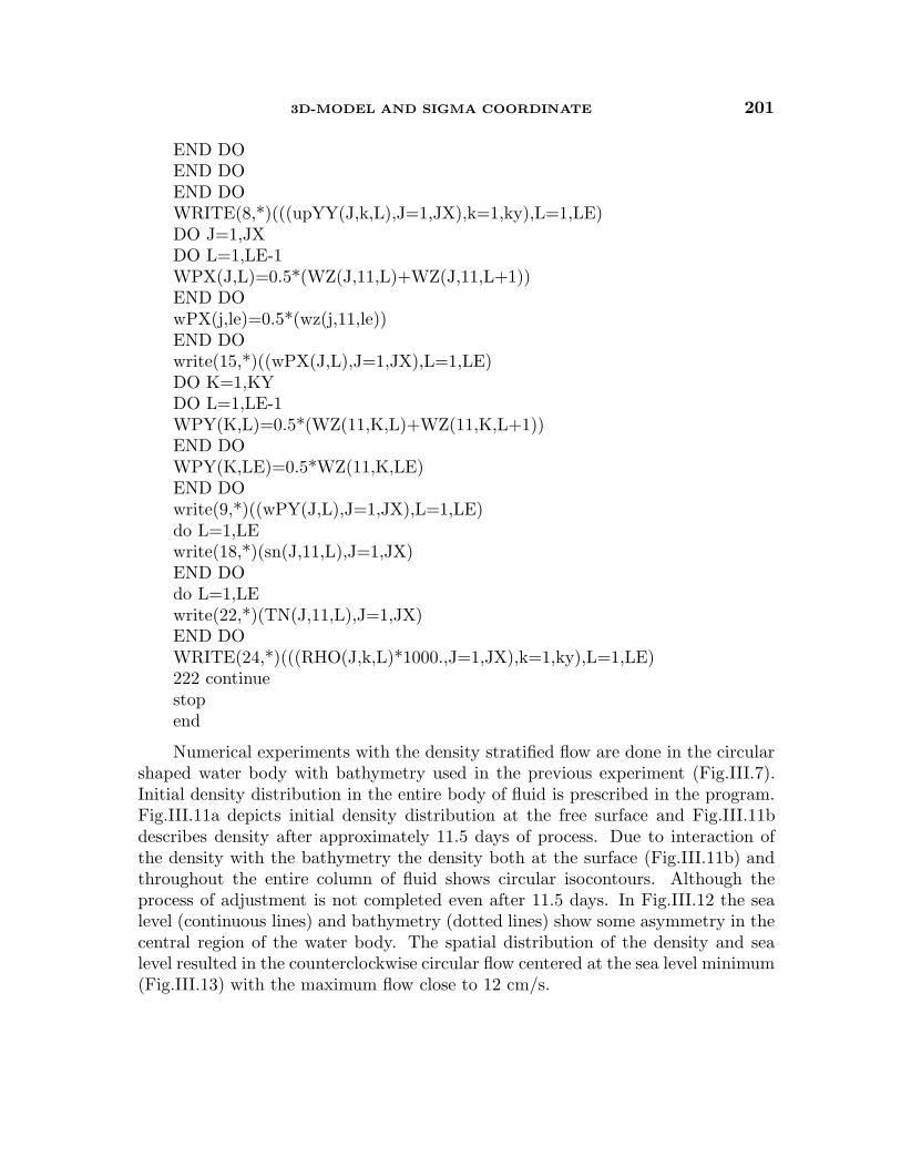
3D-MODEL AND SIGMA COORDINATE 201
END DOEND DOEND DOWRITE(8,*)(((upYY(J,k,L),J=1,JX),k=1,ky),L=1,LE)DO J=1,JXDO L=1,LE-1WPX(J,L)=0.5*(WZ(J,11,L)+WZ(J,11,L+1))END DOwPX(j,le)=0.5*(wz(j,11,le))END DOwrite(15,*)((wPX(J,L),J=1,JX),L=1,LE)DO K=1,KYDO L=1,LE-1WPY(K,L)=0.5*(WZ(11,K,L)+WZ(11,K,L+1))END DOWPY(K,LE)=0.5*WZ(11,K,LE)END DOwrite(9,*)((wPY(J,L),J=1,JX),L=1,LE)do L=1,LEwrite(18,*)(sn(J,11,L),J=1,JX)END DOdo L=1,LEwrite(22,*)(TN(J,11,L),J=1,JX)END DOWRITE(24,*)(((RHO(J,k,L)*1000.,J=1,JX),k=1,ky),L=1,LE)222 continuestopend
Numerical experiments with the density stratified flow are done in the circularshaped water body with bathymetry used in the previous experiment (Fig.III.7).Initial density distribution in the entire body of fluid is prescribed in the program.Fig.III.11a depicts initial density distribution at the free surface and Fig.III.11bdescribes density after approximately 11.5 days of process. Due to interaction ofthe density with the bathymetry the density both at the surface (Fig.III.11b) andthroughout the entire column of fluid shows circular isocontours. Although theprocess of adjustment is not completed even after 11.5 days. In Fig.III.12 the sealevel (continuous lines) and bathymetry (dotted lines) show some asymmetry in thecentral region of the water body. The spatial distribution of the density and sealevel resulted in the counterclockwise circular flow centered at the sea level minimum(Fig.III.13) with the maximum flow close to 12 cm/s.
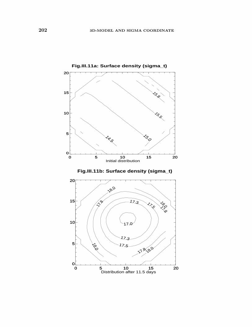
202 3D-MODEL AND SIGMA COORDINATE
Fig.III.11a: Surface density (sigma_t)
0 5 10 15 20Initial distribution
0
5
10
15
20
14.515.0
15.5
15.8
0 5 10 15 200
5
10
15
20
0 5 10 15 20 Distribution after 11.5 days
0
5
10
15
20
Fig.III.11b: Surface density (sigma_t)
17.0
17.3
17.3
17.5
17.5
17.8
17.8
17.8
18.0
18.0
18.0
18.0
0 5 10 15 200
5
10
15
20
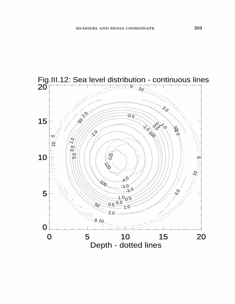
3D-MODEL AND SIGMA COORDINATE 203
Fig.III.12: Sea level distribution - continuous lines
0 5 10 15 20 Depth - dotted lines
0
5
10
15
20
2.0
2.0
2.0
1.0
1.01.
0
0.5
0.50.
5
0.0
0.0
0.0
-0.5
-0.5
-1.0
-1.0
-2.0
-2.0
3.0
-3.0-4.0
3.0
0 5 10 15 200
5
10
15
20
5
5
5
5
10
10
10
10
50
50
50
100
100120
125
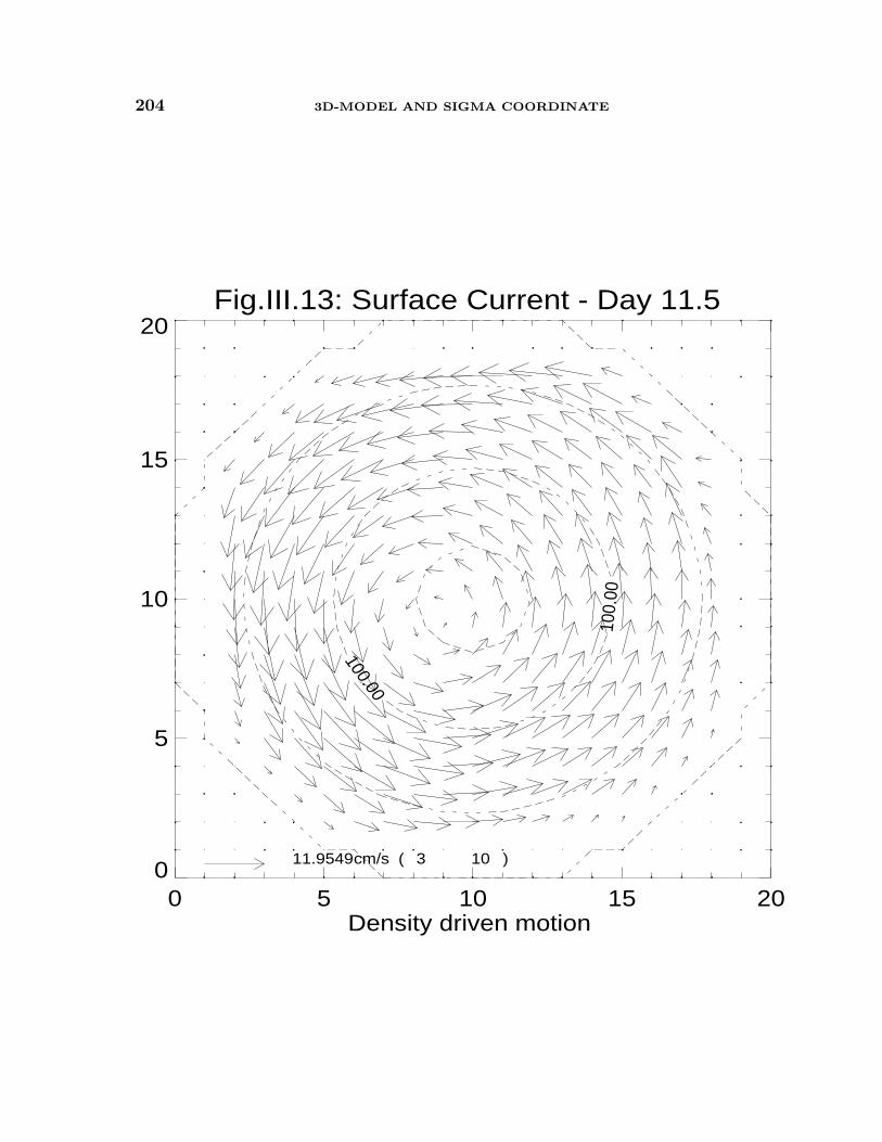
204 3D-MODEL AND SIGMA COORDINATE
Fig.III.13: Surface Current - Day 11.5
0 5 10 15 20Density driven motion
0
5
10
15
20
100.00
100.
00
11.9549cm/s ( 3 10 )
205
APPENDIX
BASIC MATHEMATICAL FORMULAS
RUDIMENTS OF TRIGONOMETRY
1. Trigonometric Functions
sin2 x + cos2 x = 1
sinx =tanx√
1 + tan2 xcosx =
1√1 + tan2 x
sin 2x = 2 sinx cosx cos 2x = cos2 x− sin2 x
sin 3x = 3 sinx− 4 sin3 x cos 3x = 4 cos3 x− 3 cosx
1 − cosx = 2 sin2 x
21 + cosx = 2 cos2
x
2
sin(x± y) = sinxcos y ± cosxsin y
cos(x± y) = cosxcos y ∓ sinxsin y
2. Hyperbolic Functions
sinhx =(ex − e−x)
2coshx =
(ex + e−x)2
cosh2 x− sinh2 x = 1
206
sinh 2x = 2 sinhx coshx cosh 2x = cosh2 x + sinh2 x
cosh x− 1 = 2 sinh2 x
2cosx + 1 = 2 cosh2 x
2
sin z = −i sinh iz cos z = cosh iz
sinh z = −i sin iz cosh z = cos iz

207
RUDIMENTS OF COMPLEX NUMBERS THEORY
1. The complex number z is defined by setting
z = a + bi,
where a and b are real numbers and i is the imaginary unit: i2 = −1.
2. The complex conjugate z of a complex number z = a + bi is defined bysetting
z = a− bi;
zz = (a + bi)(a− bi) = a2 + b2
3. To add or subtract complex numbers, we add or subtract the real andimaginary
parts separately:
(a + bi) + (c + di) = (a + c) + (b + d)i
Multiplication is defined as follows:
(a + bi)(c + di) = (ac− bd) + (ad + bc)i
To divide one complex number by another we multiply a numerator and adenominator by the complex conjugate of the denominator:
a + bi
c + di=
(a + bi)(c− di)(c + di)(c− di)
=ac + bd
c2 + d2+ i
bc− ad
c2 + d2
4. Trigonometric form of a complex number:
z = r(cosφ + i sinφ),
where r =√a2 + b2 is called an absolute value of a complex number and
φ = arctan ba is called an argument of a complex number.
5. Exponential form of a complex number:
z = reiφ
208
z = reiφ = r(cosφ + i sinφ)
z = re−iφ = r(cosφ− i sinφ)
sinφ =(eiφ − e−iφ)
2icosφ =
(eiφ + e−iφ)2

209
RUDIMENTS OF ALGEBRA
1. Quadratic Equation.
ax2 + bx + c = 0
D = b2 − 4ac
x1 =−b +
√D
2ax2 =
−b −√D
2aIf D > 0, the roots are real; x1 �= x2.If D = 0, the roots are real; x1 = x2.If D < 0, the roots are complex conjugates.
ax2 + bx + c = a(x− x1)(x− x2)
2. The linear homogeneous algebraic system of equations{a1x + b1y = 0a2x + b2y = 0
has a solution only if its determinant is equal to zero:
det =∣∣∣∣ a1 b1a2 b2
∣∣∣∣ = a1b2 − a2b1 = 0.
The same approach is valid for the 3-rd order linear algebraic system of equa-tions: {
a1x + b1y + c1z = 0a2x + b2y + c2z = 0a3x + b3y + c3z = 0
1) det =
∣∣∣∣∣a1 b1 c1a2 b2 c2a3 b3 c3
∣∣∣∣∣ = a1b2c3 + a3b1c2 + a2b3c1 − a3b2c1 − a1b3c2 − a2b1c3 = 0.
2) det =
∣∣∣∣∣a1 b1 c1a2 b2 c2a3 b3 c3
∣∣∣∣∣ = a1
∣∣∣∣ b2 c2b3 c3
∣∣∣∣ − b1
∣∣∣∣ a2 c2a3 c3
∣∣∣∣ + c1
∣∣∣∣ a2 b2a3 b3
∣∣∣∣ = 0.
210
RUDIMENTS OF POWER SERIES AND INTEGRATION
1. Newton’s binomial series
For any constant s
(a + b)s = as + sas−1b +s(s− 1)
2!as−2b2 +
s(s− 1)(s− 2)3!
as−3b3 + · · ·
Especially useful when a or b is small, e.g., if x → 0, then,
(1 − x)−1 � 1 + x
2. Maclaurin series
ex = 1 + x +12x2 +
13!
x3 +14!
x4 + ...
sinx = x− 13!
x3 +15!
x5 + .....
cosx = 1 − 12!
x2 +14!
x4 + ...
3. Integral with variable limits
∂
∂x
∫ b
a
f(x, z)dz = f(b)∂b
∂x− f(a)
∂a
∂x+
∫ b
a
∂f(x, z)∂x
dz