Word Spotting DTW

Word Spot DTWIntroductionThe Basic IdeaPruningDTWMatching Words With DTWExperimental ResultsSummary

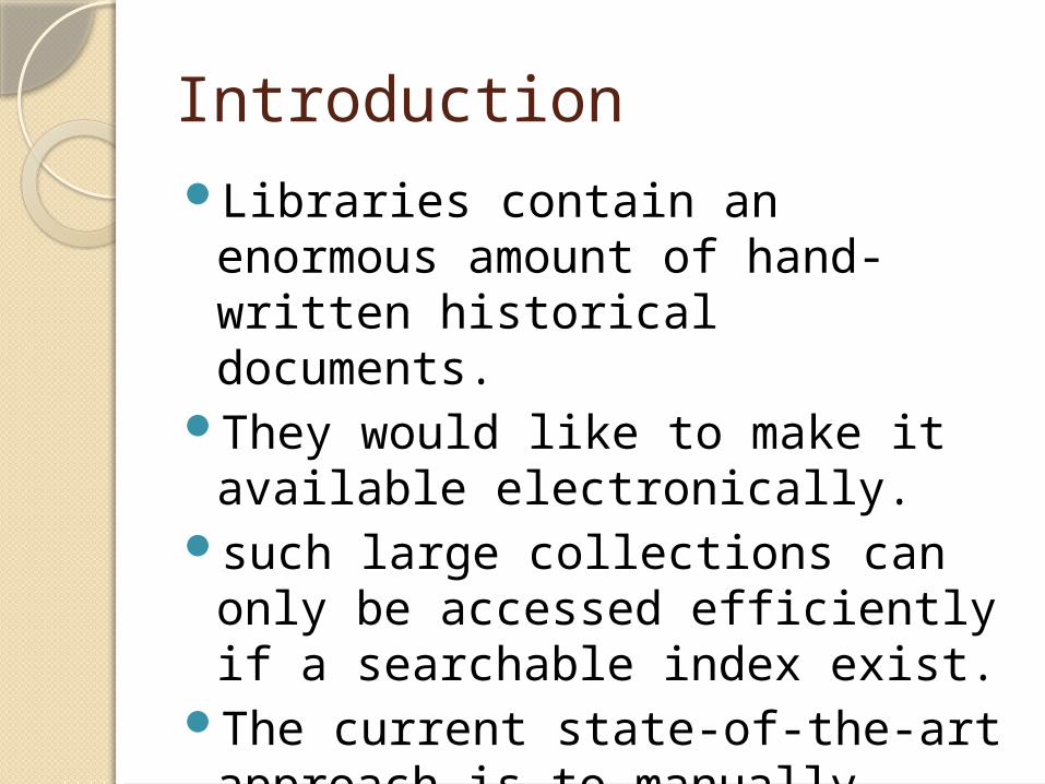
IntroductionLibraries contain an enormous

amount of hand-written historical documents.

They would like to make it available electronically.

such large collections can only be accessed efficiently if a searchable index exist.

The current state-of-the-art approach is to manually create an index.

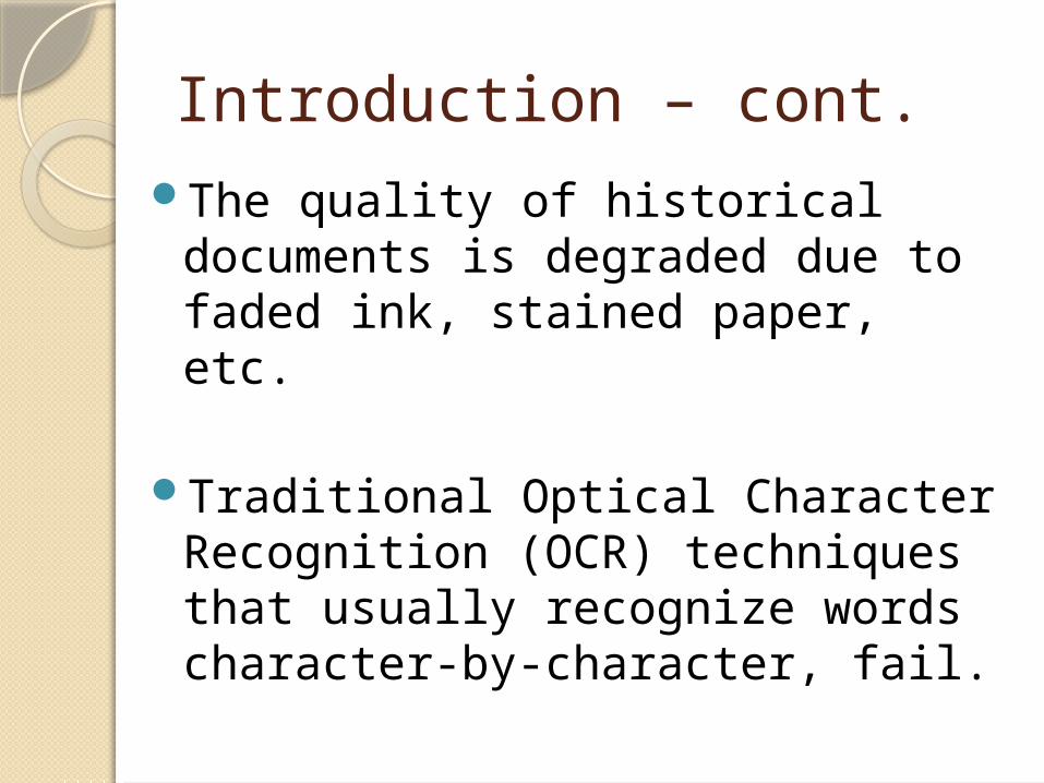
Introduction – cont.The quality of historical documents

is degraded due to faded ink, stained paper, etc.

Traditional Optical Character Recognition (OCR) techniques that usually recognize words character-by-character, fail.

Introduction – cont.

The Basic IdeaFor handwritten manuscripts

written by a single author - the images of multiple instances of the same word are likely to look similar.

Word spotting idea provides an alternative approach to index generation.

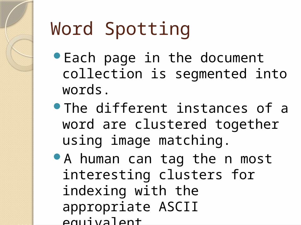
Word SpottingEach page in the document

collection is segmented into words.

The different instances of a word are clustered together using image matching.

A human can tag the n most interesting clusters for indexing with the appropriate ASCII equivalent.

MatchingGood matching performance can be

achieved by:◦ A technique that skews, resizes and

aligns two candidate words.◦Compares the words pixel-by-pixel.

We will use DTW.

PruningRunning a matching algorithm is

expensive with growing collection sizes.

Pruning techniques which can discard unlikely matches are used.

Pruning TechniquesPruning of word pairs based on

the area and aspect ratio of their bounding boxes.

Require words to have the same number of descenders (strokes below the baseline).

The idea is to require similar pruning statistics.

Upper BaselineLowerBaseline

Ascenders

Descenders

DTWUsed to compute a distance between

two time series.A time series is a list of samples taken

from a signal ordered by time.Naive approach: resample one of them

and then compare the series sample-by-sample.

does not produce intuitive results, as it compares samples that might not correspond well.

DTWRecovering optimal alignments

between sample points in the two time series.

Demonstrates:

time

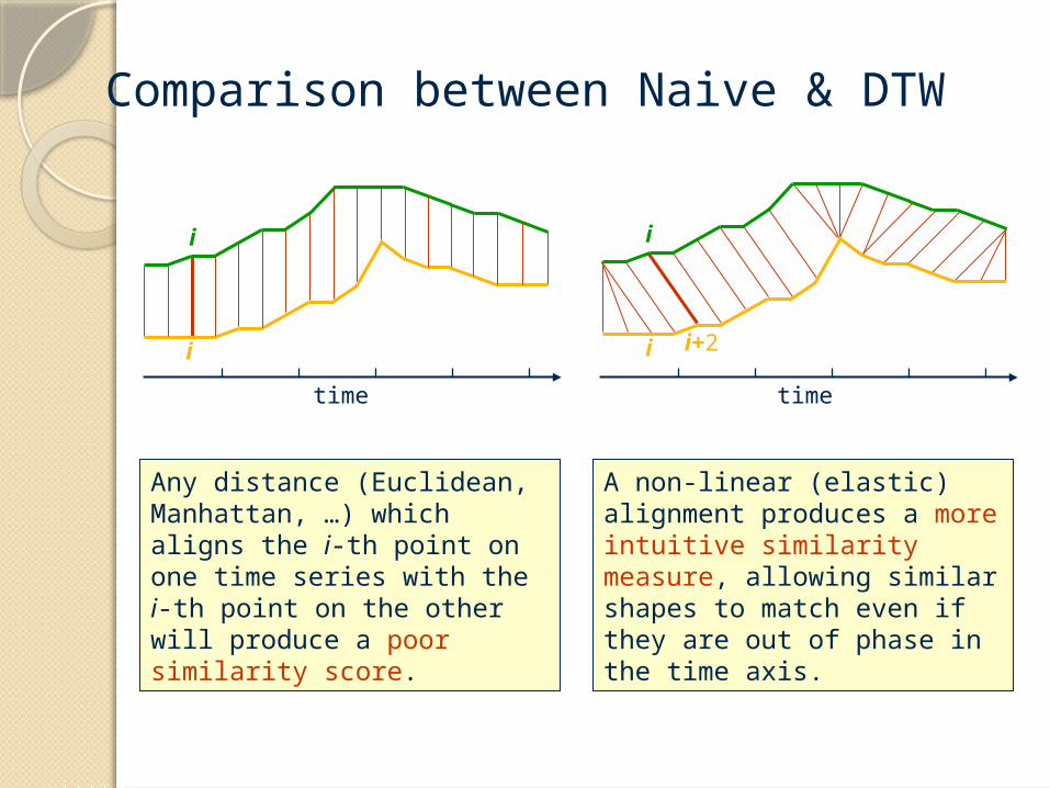
Comparison between Naive & DTW

i

i

time

Any distance (Euclidean, Manhattan, …) which aligns the i-th point on one time series with the i-th point on the other will produce a poor similarity score.

i

i+2i

time

A non-linear (elastic) alignment produces a more intuitive similarity measure, allowing similar shapes to match even if they are out of phase in the time axis.

DTWThe DTW-distance between two time

series Xi . . . Xm and Yi . . . Yn is D(m,n).

D(i,j)= min {D(i,j-1),D(i-1,j),D(i-1,j-1)} + d(i,j)

d(i,j) varies with the application.This calculation realizes a local

continuity constraint.

js

is

m

1

n1

Time Series B

Time Series A

pk

ps

p1

To find the best alignment between A and B one needs to find the path through the grid

P = p1, … , ps , … , pk

ps = (is , js )

which minimizes the total distance between them.

P is called a warping function.

Warping Function

Time-Normalized Distance Measure

D(A , B ) =

k

ss

k

sss

w

wpd

1

1

)(

d(ps): distance between is and js

Pminarg

ws > 0: weighting coefficient.

Best alignment path between A and B :

Time-normalized distance between A and B :

P0 = (D(A , B )).

js

is

m

1

n1

Time Series B

Time Series A

pk

ps

p1

Matching words with DTW

Matching words with DTWThe inter-character and intra-character

spacing is subject to larger variations.DTW offers a more flexible way

compensate for these variations than linear scaling.

We first normalize the slant and skew angle of candidate images.

From each word, four features per image column are extracted and combined into a single time series.

Matching Words With DTWFor each image I with height h

and width w, we extract a time series:◦X(I) = x1….xw.

◦xi = f1(I,i),f2(I,i),f3(I,i),f4(I,i).

◦ fk = four extracted features per image column.

Matching Words With DTWIn order to run the DTW algorithm

on two time series X(I) and Y(J), we define a local distance function:◦d(xi,yj ) = ∑ (fk(I,i)-fk(J,j))²

Now, the DTW algorithm can be run to determine a warping path between X and Y:◦D(X,Y) = ∑ d(xik,yjk )

DTW FeaturesProjection ProfilesWord Profiles

◦Upper word profiles◦Lower word profiles

Background/Ink transitions

Projection ProfileProjection profile capture the

distribution of ink along one dimension in a word image.

A vertical projection profile is computed by summing the intensity values in each image column separately:◦PP(I,c) = ∑ (255-I(r,c))

r=1

h

(a) original image: slant/skew/baseline-normalized, cleaned.

(b) normalized projection profile.

Word ProfilesWord profiles capture part of the

outlining shape of a word.Using upper and lower word profiles.Going along the upper (lower)

boundary of a word’s bounding box.Recording for each image column

the distance to the nearest “ink” pixel in that column.

Word ProfilesDue to a number of factors, some

image columns may not contain ink pixels.

Therefore, these gaps are closed by linearly interpolating between the two closest points.

Upper Boundary

Lower Boundary

Background/Ink Transitions

A capture of the inner structure of a word is missing.

Records for every image column, the number of transitions from the background to ink pixels: ◦Determined by threshold.◦nbit(I, c).

Experimental ResultsData sets and processingResults

Data Sets And Processingconducted on two test sets of

different quality◦Acceptable quality (set 1).◦Very degraded quality (set 2).

Divide the test to four sets:◦15 images in test set 1.◦Entire test set 1.◦32 images in test set 2.◦Entire test set 2.

Test Sests

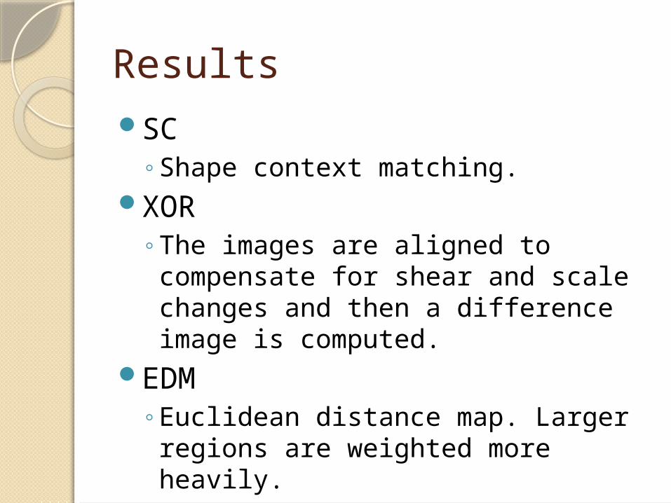
ResultsSC

◦Shape context matching.XOR

◦The images are aligned to compensate for shear and scale changes and then a difference image is computed.

EDM◦Euclidean distance map. Larger

regions are weighted more heavily.

ResultsTest set/Algorithm

XOR SSD SLH SC EDM DTW

A 54.14% 52.66% 42.43% 48.67% 72.61% 73.71%

B n/a n/a n/a n/a n/a 65.34%

C n/a n/a n/a 48.11% 49.56% 58.81%

D n/a n/a n/a n/a n/a 51.81%

Summary & ConclusionsDTW approach perform better than

a number of other techniques.◦Accuracy. ◦Speed.

The future work will focus on improvements in speed and accuracy.◦Pruning.◦Optimizations in DTW.