Women in Politics: Evidence from the Indian states Irma...

Women in Politics: Evidence from the Indian states

Irma Clots-Figueras

London School of Economics and STICERD

Political Economy and Public Policy Series The Suntory Centre Suntory and Toyota International Centres for Economics and Related Disciplines London School of Economics and Political Science Houghton Street London WC2A 2AE

PEPP/14 October 2005 Tel: (020) 7955 © The author. All rights reserved. Short sections of text, not to exceed two paragraphs, may be quoted without explicit permission provided that full credit, including © notice, is given to the source

Women in Politics. Evidence from the Indian states∗

Irma Clots-Figueras†

London School of Economics and STICERD

January 24, 2005

Abstract

This paper uses panel data from the 16 main states in India during the period 1967-1999 to study the effects of having higher female representation in the State Legislatureson public goods, policy and expenditure. I find that women legislators make different deci-sions than men legislators. Moreover, women elected in seats reserved for scheduled castesand tribes make different decisions compared to women elected in general seats. Sched-uled caste/tribe women favour capital investments, especially on low tiers of education andirrigation. They also favour “women-friendly” laws, such as amendments to the HinduSuccession Act that give women the same inheritance rights as men. In contrast, generalwomen legislators do not have any impact on “women-friendly” laws, oppose redistribu-tive policies such as land reforms, favour pro-rich expenditure and invest in high tiers ofeducation.

JEL classification: D70, H19, H41, H50,O10.Keywords: gender, caste, panel data, policy, India.

1 Introduction

In India, as in many other countries in the world, women are underrepresented in all politicalpositions, even if they form approximately one half of the population. While the proportionof women who went to vote increased during the 1990s, women are still not well representedin political life. In a representative democracy all sectors of the society should have a voicein policy making. But, does women representation matter for policy determination? Doparliaments where women have higher representation adopt different policies?

This paper studies how women political representation influences expenditure, public goodsand policy decisions using panel data from the 16 main states in India during the period 1967-1999.

∗I am indebted to Oriana Bandiera for her help and for very useful comments and suggestions. I am alsograteful to Tim Besley and Robin Burgess for very useful comments and the data provided. I also thank allthe EOPP seminar participants at the London School of Economics, at the ESPE 2004 conference and at theEEA-ESEM annual conference 2004. All errors are mine.

†email:[email protected]. Correspondence: STICERD-LSE, Houghton Street, WC2A 2AE London,UK.

1

In political economy models where candidates can commit to specific policies and onlycare about winning, political decisions only reflect the electorate’s preferences (Downs (1957)).In this sense, women political representation should not have a differential impact on policydecisions as the median voter equilibrium prevails. In fact, as long as women vote, theirpreferences would be represented by the candidate elected, irrespective of this candidate’sgender. However, if complete policy commitment is absent the identity of the legislator mattersfor policy decisions (Besley and Coate (1997); Osborne and Slivinski (1996)). In particular,increasing a group’s political representation will increase its influence in policy.

The issue of women political representation has been increasingly important in India. InSeptember 1996, the Indian Government introduced a Bill in Parliament, proposing the reser-vation of one third of the seats for women in the Lok Sabha (Central Government) and theState Assemblies. Since then, this proposal has been widely discussed in several parliamentarysessions, without an agreement being reached. Those who are in favour of this reservationargue that increasing women’s political representation will ensure a better representation oftheir needs. Even those who oppose the reservation acknowledge the fact that women politi-cians behave differently than men politicians. Clearly, reservation would change the natureof political competition, by changing the set of candidates available for each seat, by alteringvoters’ preferences or by changing the candidates’ quality. This paper explores the effect of anexogenous increase in women representation that took place without any institutional change,and allows me to clearly identify the effect of women legislators in the variables of interest.

I focus on state governments as these control most of the social and economic expenditureand have the power to implement most of the development policies in India. Importantly, thedifferent Indian states use the same budgetary classification, and have similar institutional andelectoral settings. Thus, using panel data from these states not only offers the advantageof data comparability, it also solves the unobserved heterogeneity problems present in cross-country studies.1

In India some seats can only be contested by scheduled caste or scheduled tribe candi-dates. These two population groups constitute the most disadvantaged sector of the Indiansociety, both socially and economically. Since scheduled caste and scheduled tribe (henceforth,SC/ST) women legislators might have different preferences than women legislators who wonthe elections for general seats, the impact of both general and SC/ST women legislators will beidentified separately2. Moreover, if the cost of running for election is higher for women than formen, women legislators will probably belong to the elite. This will only be the case for generalwomen legislators, since scheduled tribes and scheduled castes are a more homogeneous group.Thus, the fact that some seats are reserved for low castes allows me to identify separately theeffect of low caste women legislators and to distinguish the gender effects from the class effects.

The identification strategy used in this paper takes advantage of the detailed data I havecollected on women candidates in India from 1967 until 2001. It is based on the fact that women

1These 16 states account for more than 95 per cent of the total population in India, about 804 million people.They are Andhra Pradesh, Assam, Bihar, Gujarat, Haryana, Jammu & Kashmir, Karnataka, Kerala, MadhyaPradesh, Maharashtra, Orissa, Punjab, Rajashtan, Tamil Nadu, Uttar Pradesh and West Bengal.

2Empirical evidence shows that almost no women SC/ST contested for a general seat and won the election,thus, I can safely say that all female legislators contesting the elections for a general seat belong to higher castesthan female legislators contesting the election for a SC/ST seat.

2

candidates who won in a close election against a man will be elected in similar constituenciesand under similar circumstances than men candidates who won in a close election against awoman. The fact that a man or a woman candidate wins in a close election can be consideredto a high extent random, and thus, the gender of the legislator effect can be correctly identifiedby comparing “treated” constituencies where a woman was elected to its “counterfactuals”,where a man was elected.

In order to have a complete picture of the effect of women legislators, I have collecteddetailed data on the Revenue and Capital budgets, to identify the expenditure priorities ofthese legislators. I also use data on public goods and two types of laws, one that is targetedtowards the poor and another one which is targeted towards women.

I find that women legislators have a differential impact on public goods, policy and ex-penditure decisions if we compare them to their male counterparts. Moreover, whether thesewomen legislators belong to a scheduled caste (SC) or scheduled tribe (ST) reserved seat alsohas an impact. In particular, scheduled caste and scheduled tribe women legislators favourcapital investments, especially on irrigation and low tiers of education, and increase revenueexpenditure on water supply. They also favour “women-friendly” laws, such as amendmentsto the Hindu Succession Act, designed to give women the same inheritance rights as men. Onthe other hand, general women legislators do not have any impact on “women-friendly” laws,oppose redistributive policies such as land reforms, favour pro-rich expenditure, invest in hightiers of education and reduce social expenditure.

This paper contributes to a larger literature that analyses similar issues using US data.Thomas (1991) shows how states with higher female representation in parliament introduceand pass more priority bills dealing with issues of women, children and families than theirmale counterparts or women in states with lower female representation. Thomas and Welch(1991) find that women in state houses in 12 states in the US place more priority than men onlegislation concerning women, family issues and children. Case (1998), finds how the state’schild support enforcement policies tightened as the number of women legislators in the stategrew. Besley and Case (2000) show that the fraction of women in state upper and lowerhouses are highly significant predictors of state workers compensation policy. Besley and Case(2002) find that women in the legislature apply pressure to increase family assistance, and tostrengthen child support laws . Rehavi (2003) finds that an increase in female representationduring the 1990’s leads to an increase in Public Welfare Expenditure. This paper complementsthis literature by identifying the gender and class of the legislators separately and finding thatboth matter for policy decisions.

The existing literature on India focuses on the effect of different reservation policies. Chat-topadhay and Duflo (2004) show how the reservation of one third of the seats for women inPanchayats (local rural self-government) of West Bengal and Rajasthan has a positive impacton investment in infrastructures relevant to women’s needs. Pande (2003), analyses how thereservation of seats for scheduled castes and scheduled tribes in the State Assemblies increasesthe volume of transfers that these groups receive. My paper studies the different effects ofvariation in both scheduled caste/tribe and general women representation due to electoraloutcomes rather than reservation policies.

The remainder of the paper is organized as follows. Section 2 explains the institutionalbackground. Section 3 describes the data. Section 4 discusses the econometric strategy. Section

3

5 presents the results and Section 6 concludes.

2 Institutional background

India is a bicameral parliamentary democracy. The lower house is called Lok Sabha, andhas 545 members. The upper house is called Rajya Sabha, and has 250 members. India is afederal country, and the Constitution gives the states and union territories significant controlover their own government.

The Vidhan Sabhas (Legislative Assemblies) are directly elected bodies that carry out theadministration of the government in the 25 states of India. In some states there is a bicameralorganization of legislatures, with both an Upper and Lower House. However, it is the LowerHouse (Legislative Assembly) the one that takes the final budget decisions. The Vidhan Sabhas,or State Legislative Assemblies, have the freedom to decide the budget they will allocate todevelopment policies.

Because of the nature of Indian federalism, state governments are the appropriate unit ofanalysis. In a process of decentralization, the states have replaced the central government inthe economic decision making. The idea is that these decisions should be taken by lower levelsof government, that are more directly responsible to its citizens.

In the event of elections, the states and union territories are divided into single-memberconstituencies. The boundaries of assembly constituencies are drawn to make sure that thereare, as near as practicable, the same number of people in each constituency. The Assembliesvary in size, according to population.

Electors can cast one vote each for a candidate the winner being the candidate who getsthe highest number of votes.

The democratic system in India is based on the principle of universal adult suffrage, andany Indian citizen who is registered as a voter and is over 25 years of age is allowed to contestelections to the Lok Sabha or State Legislative Assemblies. Candidates for the Vidhan Sabhashould be a resident of the same state as the constituency from which they wish to contest.

The 1950 Indian Constitution provides for political reservation for scheduled castes andscheduled tribes. According to articles 330 and 332 of the constitution, prior to every nationaland state election, a number of jurisdictions will be reserved for these groups. Both scheduledcastes and scheduled tribes tend to be socially and economically disadvantaged, and theyconstitute about 25% of the total population in India. There are two criteria for the reservationof jurisdictions: the population concentration of SC/ST groups in that constituency and thedispersion of reserved jurisdictions within a particular state.

Women belonging to scheduled castes and scheduled tribes are those who suffer a majordegree of discrimination in India. Being a particularly disadvantaged within the Indian socialstructure, they will have different preferences than the other legislators in the State Assemblies.On the other hand, political parties seem to propose more women candidates for SC/ST seatsthan for general seats. Due to these reasons, and due to the fact that many general womencandidates belong to the elite, I estimate separately the effects of these legislators on thedifferent expenditure, public goods and policy measures under study.

In each one of the states, the budget is approved by the legislature after the enactment

4

of the Appropriation Act which gives authority to the government to withdraw money fromthe Consolidated Fund.3 Usually a budget speech is given to the legislature by the FinanceMinister of each state, two days after there is a general discussion in the legislature about thebudget proposal presented. This discussion lasts 6 days. After that, and during a maximumperiod of 18 days, individual demands made by the individual legislators are voted in theLegislative Assembly. Then, the introduction, consideration and passing of the AppropriationBill in the Legislative Assembly with the Governor’s consent lasts for about two days. In total,the budget discussion takes a maximum of 26 days.

3 Data Description

I use data on the sixteen main states in India during the period 1967-1999. Tables A1-A4report descriptive statistics of the variables used. My aim is to test the effects of having higherfemale representation in the State Legislatures on revenue and capital expenditure, publicgoods and policy. I also test whether women legislators in scheduled caste or scheduled tribeseats (SC/ST) have a different impact than those in general seats.

The electoral data has been collected from the different reports on the State Electionspublished by the Election Commission of India.

As an indicator for female representation in general seats I use the fraction of the totalnumber of general seats in the State Legislature occupied by a woman legislator for each stateand election.

As an indicator of female legislators in SC/ST seats I use the fraction of the total numberof SC/ST seats occupied by a female legislator. The fraction of seats serves as an indicator ofthe relative power of these state legislators.

The data on individual candidates for the state elections in India from 1967-2001 allowsme to calculate how many candidates were involved in a close election4 against a candidate ofthe opposite sex for each state and year and for both SC/ST and general seats. I also use thefraction of seats won by each political party.

All the electoral data used in this paper has been collected from the different StatisticalReports of the Election Commission of India. Figure (1) in the Appendix shows the variationacross election years and states for both SC/ST and general women representation. Womenrepresentation has been low in all states during the time period under consideration, both forSC/ST and general seats. In fact, at most 24% of the SC/ST seats and 14% of the generalseats have been won by a woman in an election between 1967-2001.

Despite the fact that women political representation is very low for all states in India, bothgeneral and SC/ST women representatives are shown to have an effect on both capital andrevenue expenditure, public goods and policy decisions. Due to the way decisions are taken inthe State Legislatures in India, even if female legislators do not constitute a “critical mass” in

3Defined by the Constitution as ”all revenues received by Government, all loans raised by Government byissue of treasury bills, loans or ways and means advances and all money received by Government in repaymentof loans”.

4A close election is defined as one in which the winner won the runner up by a very small margin. In thispaper I define close elections as those in which the margin was less than 2.5%.

5

any voting procedure, they can still convince other legislators during or before the discussions,and they can also introduce proposals that are then voted by the legislature. Mishra, R.C.(2000), shows how evidence from the debates in the Orissa Legislative Assembly indicates thatwomen legislators introduce proposals in the legislature, participate in the debates and tryto convince their male counterparts of their ideas. This is true for both general and SC/STwomen legislators. Moreover, they could as well be the ”swing vote” when a given decision istaking place.

3.1 Dependent Variables

I study the impact of female legislators on different components of the state budget. For thisI have collected data on actual Revenue and Capital expenditure for each state and year.

Revenue expenditure is defined as expenditure on current consumption of goods and ser-vices of the departments of Government, expenditure on Legislature, State Administration, taxcollection, debt servicing and interest payments and grants-in-aid to various institutions. Cap-ital expenditure is defined as expenditure devoted to acquiring or creating assets of a materialand permanent character or to reduce recurrent liabilities.

Revenue expenditure in each one of the state’s budgets is divided among two main cat-egories: Development expenditure and Non-Development expenditure. Development expen-diture is money allocated to the maintenance of capital assets, both economic and social.Non-Development expenditure is directed towards current and consumption expenditures ofthe government.

Total Capital Disbursements are divided into two main categories: Total Capital Outlayand Discharge of Internal Debt. Total Capital Outlay is mainly composed of Developmentexpenditure, which includes both Social and Economic Services. Discharge of Internal Debtincludes different types of loans. Figure 2 in the appendix shows graphically how all thedifferent expenditure categories are organized in both the capital and the revenue budgets inall the Indian states.

I use the share of Total Revenue expenditure and the share of Total Capital Disbursementsdevoted to each type of expenditure as an expenditure measure. Summary statistics for theexpenditure variables appear in Tables A2 and A3 in the appendix. Results in this paper arefor the 12 biggest subdivisions in each one of the budgets.

All the states in India use the same budgetary classification. The variables are deflatedusing the Consumer Price Index for Agricultural Labourers (CPIAL) and the Consumer PriceIndex for Industrial Workers (CPIIW). The reference period used is October 1973-March 1974.

I also use some public goods measures. As educational measures I use the total numberof schools and the number of secondary, middle, and primary schools per every thousandindividuals. This will give an approximate idea of the supply of education. I also use thenumber of teachers per thousand individuals. Data on kilometres of surfaced state roads perkm2 is used as a measure of infrastructure.

The policy variables I use are cumulative number of land reforms designed to tackle povertyenacted by the different states in India during 1967-1999. The types of land reforms used areTenancy Reforms, Abolition of Intermediaries reforms and Land Ceiling legislation.5

5 I use the land reform measure created by Besley and Burgess (2000). Details on this variable can be found

6

The “women-friendly” policy variable I use is a dummy variable which equals one the yeara given state has made an amendment to the Hindu Succession law to ensure that both womenand men have the same inheritance rights.

3.2 Control variables

Control variables in the regressions include the proportion of seats won by each one of theparties in each election, in order to distinguish the effect of gender from the effect of partyideology6.

Other control variables include the real net state domestic product per capita, total grantsreceived by the central government in real per capita terms, population in each state, the shareof rural population over total population and a dummy for the year before the elections tookplace.

All these variables could affect the dependent variable in different ways: the higher theamount of grants received by the state, the higher will be their expenditure capacity, and thiscan affect their expenditure decisions. On the other hand, the population variables and realper capita state net domestic product could also give an idea of the economic backwardness ofthe state, which can also influence the policy decisions adopted.

The dummy variable for the year before the elections takes into account that legislatorsmight adopt different policies just before elections, in order to increase their probability ofbeing re-elected. I also include a time trend in the regressions.

Since in 1985 there was a budgetary reclassification, I also include a dummy variable forthe years before 1985 in the expenditure regressions. This will be specially relevant for theEconomic expenditure in the Revenue Account, since this was the expenditure category whichchanged the most after the reclassification took place. Another budget reclassification tookplace in 1972, however, budget data for the period 1967-1972 can not be safely compared forall the expenditure categories to budget data from later periods. For this reason I focus on thetime period 1972-1999 for the expenditure variables.

4 Econometric Specification

To analyse the effects of having higher female representation in both SC/ST and general seatsin the State Assemblies in India on government expenditure, public goods and policy measures,I use panel data for the 16 main states in India during the period 1972-1999.

The first empirical specification is:

there.6There are eight main party groups: Congress, Hard Left, Soft Left, Janata, Hindu, Regional, Independent

candidates and other parties. Congress parties include Indian National Congree Urs, Indian National CongressSocialist Parties and Indian National Congress. Hard Left parties include Communist Party of India andCommunist Party of India Marxist Parties. Soft Left parties include Praja Socialist Party and Socialist Party.Janata parties include Janata, Lok Dal, and Janata Dal parties. Hindu parties include the Bharatiya JanataParty. Regional parties include Telegu Desam, Asom Gana Parishad, Jammu & Kashmir National Congress,Shiv Sena, Uktal Congress, Shiromani Alkali Dal and other state specific parties.

7

Yit = αi + βt + γWit + δXit + uit (1)

Where Yit is the measure of expenditure, public goods or policy for state i in year t. αiand βtare state and year fixed effects, Wit is the fraction of seats occupied by women in thestate assemblies elected in the previous elections, and Xit stands for other control variablesincluded in the regression which vary over state and over time and can also have an effect onthe dependent variables of interest.

For the election years I use female representation as it was in the previous elections, underthe assumption that newly elected legislators might not have much power during the firstelection year.7 Moreover, some of the elections are held at the end of the year, when decisionshave already taken place.

The year fixed effects control for nationwide shocks or policies that were implemented inall states at the same time. The state fixed effects control for state specific characteristics thatdo not vary over time.

Since women legislators who won the election for a general seat might have different policypreferences than women legislators who won the election for a SC/ST seat, I include bothgeneral and SC/ST women representation variables in the regression. Moreover, in this wayI can provide more evidence on the difference between gender and class effect. If the costof running for election is higher for women than for men politicians, women legislators willbe of comparatively higher classes than men legislators. Thus, the women representationvariable may only indicate class, not gender. India provides the opportunity of dividing thewomen representation variable among general and SC/ST legislators. The latter, being asocially and economically disadvantaged group will be more homogeneous, and thus, SC/STwomen legislators will be directly comparable to SC/ST men legislators. General legislatorsare not such an homogeneous group, and thus, gender and class effects could be confusedwhen comparing women and men politicians. Moreover, the comparison of SC/ST and generalwomen legislators is very interesting by itself, since it provides evidence that the identity ofthe legislator is defined by both gender and caste. The equation I am then testing is:

Yit = αi + βt + λWgenit + θWscstit + δXit + uit (2)

Where, as before, αi and βt are the state and year fixed effects and Xit are other controls.Wgenit is the fraction of general seats won by women as elected in the previous elections andWscstit if the fraction of SC/ST seats won by women as elected in the previous elections.

Even though the state fixed effects control for permanent differences across states in femalerepresentation and the outcome variables, I can not rule out the existence of an omitted variablethat varies over states and over time and affects both female representation and the outcomevariables. Thus, there might be some endogeneity concerns. In this case, the OLS estimatesreported in this econometric specification would be biased and specifications (1) and (2) would

7Results are robust to including the contemporaneous women representation variable in the election years.Results are available from the author.

8

not allow me to correctly identify the effect of having higher women representation on thedependent variables of interest.

To be clear, if women are elected in constituencies where there is a “preference for womenpoliticians”, this variable might also affect the dependent variables in my regressions, thus,biasing the results obtained.

As reported in Table A5 in the appendix, however, states where female representation isabove the median and states where female representation is below the median do not differon variables that might be correlated with “preference for women politicians”. States aboveand below the median are very similar in both male and female literacy rates, infant mortalityrates, income inequality, newspaper circulation per capita, the percentage of voters who arewomen and voter turnout.

To identify the effect of women legislators on the variables of interest I have collected dataon the votes’ share received by each one of the women candidates in state elections in Indiaduring then period 1967-2001, together with the margins of votes obtained against the winneror, in the case they won the elections, data on the runner-ups and the margin of votes obtainedagainst them .

I can then use the information on women candidates who barely won the elections againsta man. This should happen in constituencies where there is no clear “preference for women”politicians. If we consider that the last few votes received by both candidates are random,both the women and the men candidates could have won the elections and, thus, the fact thatthe woman candidate won the seat instead of the man is random as well.

This identification strategy is based on the regression discontinuity approach, although itis not directly used in this study.8 The fact that there have been close elections between awoman and a man candidate generates “near-experimental” causal estimates of the effect thatwomen political representation has on the policy variables.9

The second type of regressions I run are based on these assumptions. In fact, I take as aseparate explanatory variable the fraction of women who barely won the elections against aman over the total number of seats, for total women representation and for both general andSC/ST seats as follows:

Yit = αi + βt + γ1Wcloseit + γ2Wnocloseit + δXit + uit (3)

Yit = αi + βt + λ1Wgencloseit + λ2Wgennocloseit + θ1Wscstcloseit + θ2Wscstnocloseit + δXit + uit(4)

These two specifications are very similar to (1) and (2), but the political representationvariables are partitioned as follows: Wcloseit is the fraction of total seats won by women who

8For this I should be able to relate each particular legislator to an expenditure measure number. Since inIndia, State Assemblies are composed by many legislators who choose a single expenditure measure each year,I had to rule out the discontinious regression and exploit the discontinuity in the OLS regression.

9Lee(2003) takes advantage of close elections to generate “near-experimental” causal estimates of the electoraladvantage to incumbency using the discontinuous regression approach.

9

won in a close election against a man. Wnocloseit is the fraction of seats won by womenwho did not win in a close election against a man.Wgencloseit is the fraction of general seatswon by women in a close election against a man. Wscstcloseit is the fraction of SC/ST seatswon by women who won in a close election against a man, while the analogous is true forWgennocloseit and Wscstnocloseit. The residual category will thus be men legislators whodid not win in a close election against a woman legislator.

The close elections women representation variables account for the “exogenous” women,those who won the elections in constituencies where there is no clear “preference for women”politicians. Thus, if these variables have significant coefficients, this will mean that my resultsare not driven by reverse causality, and that the identity of the legislator, in this case definedby gender and caste, matters for policy decisions.

However, the no close election women representation variables account for women whoeither won against a woman or against a man in an election that is not close. Thus, theyare women who were elected in constituencies where there might be a “preference for womenlegislators”, and the coefficients of these variables can be driven by reverse causality.

In other words, the omitted variable would be correlated with the fraction of seats won bywomen in an election that is not close, but not with Wcloseit, Wscstcloseit and Wgencloseit,allowing me to identify the effect of these legislators. In this paper I define close elections aselections in which the votes difference between the winner and the runner-up is less than 2,5%of the total votes in that particular constituency.10

Since there might be the case that people who won their seats in a close election behavedifferently than those who won by bigger margins, the coefficients for women who won in aclose election against a man could be biased. In order to control for this I also include in theregressions the fraction of men who won in a close election against a woman:

Yit = αi + βt + γ1Wcloseit + γ2Wnocloseit + µMcloseit + δXit + uit (5)

Yit = αi + βt + λ1Wgencloseit + λ2Wgennocloseit + θ1Wscstcloseit + θ2Wscstnocloseit +

+µ1Mgencloseit + µ2Mscstcloseit + δXit + uit (6)

Where now Mcloseit is the fraction of seats won by a man in a close election against awoman as in the previous elections, Mgencloseit is the fraction of general seats won by a manin a close election against a woman as elected in the previous elections andMscstcloseit is thefraction of SC/ST seats won by a man in a close election against a woman as in the previouselections.

Men who won in a close election are as well likely to behave differently than those whowon by a larger margin. By testing whether the coefficients for men and women who won inclose elections are the same, I can separate the effect of women legislators from the effect oflegislators who won in close elections.

Constituencies where a woman won in a close election against a man are considered as“treated”, while those in which the men won are the “counterfactual”, since the fact thatthe woman did not win the seat is random. In other words, “treated” and “counterfactual”10 I have also defined close elections as those in which the margin was less than 2% or 1,5% of total votes.

Results are mostly unchanged.

10

constituencies will be similar in all the unobservables, they only differ in the fact that bychance either a man or a woman won the election. In specifications (5) and (6), the variablescorresponding to women and men who won in close elections account for the fraction of totallegislators which are “treated” and “counterfactual” respectively.11

There might be concerns that two different constituencies in which a woman contested in aclose election against a man might not be comparable if in one of them there were many otherwomen candidates contesting for the same seat. That would be a case in which political partiesperceive that constituency as “women friendly” and tend to field women candidates on thatparticular constituency. If the number of women candidates contesting for the same seat as thetwo close candidates is significantly different for constituencies in which a man won in a closeelection against a woman and constituencies in which a woman won in a close election againsta man, these two types of constituencies might not be comparable. As it is shown in Table A6in the appendix, the number of other women candidates contesting against women who won inclose elections against a man is not significantly different than that for men who won in closeelections against a woman, and thus, this seems not to be a concern in this study. This is thecase because the bias would be the same for both treated or non-treated constituencies.

On the other hand, it might be possible that women (or men) candidates in a close electionare in this situation because one of them is the incumbent for that seat in that particularconstituency. If this is the case, the variables for women and men legislators who won in aclose election would not be directly comparable. Moreover, the policies applied by candidateswho were the incumbent and won the elections again might be different than that of candidateswho occupy the seat for the first time. However, as it is shown in Table A6 in the appendix,the percentage of winners in close elections who were the incumbent is statistically the samefor women and men legislators. In addition, the percentage of candidates in close electionswho were the incumbent is the same for women and men as well. Thus, incumbency in closeelections seems not to be important for this study.

There might as well be concerns that the party composition in seats won in a close electionbetween two candidates of different gender may not be the same as the party compositionin the whole State Assemblies. That is, if some parties are more likely to contest and winin close elections, then results might only indicate differences in party platforms of partiescontesting close elections rather than gender effects. I have compared the variables indicatingthe proportion of seats won by the different parties in the State Assemblies and the proportionof seats won by the different parties in close elections for the states and years in which theywere close elections and the distribution of seats among parties is almost the same.12

I have also included the proportion of scheduled caste and scheduled tribe population ineach state as a control in the regressions. For this I had to restrict the observations to thosebetween 1972-1992, since I only have this population data until 1992. Results were unchanged.

The identification strategy used in this paper crucially relies on the random assignmentof the winner in a close election between a man and a woman candidate. I have tested thisassumption by regressing the probability of a woman winning in a close election on different

11Rehavi (2003) uses the fraction of close elections between a woman and a man won by a woman as aninstrument.

12Results available from the author upon request.

11

variables that could presumably affect the outcome of a woman winning the election, like bothmale and female literacy rates, real per capita net state domestic product, infant mortalityrates, newspaper circulation per capita, political competition, the fraction of votes obtainedby the Congress party, the fraction of Hindu and Muslim population and both rural and urbanheadcount ratios. None of the above coefficients were significant13.

5 Results

5.1 Capital Expenditure

Total Capital Disbursements can be divided into Total Capital Outlay and Discharge of InternalDebt. In this study I will mainly focus in Total Capital Outlay, which is the part of capitalexpenditure invested in the creation of capital goods. Discharge of Internal Debt includes bothloans repaid and advances given by the state governments, which makes it difficult to compareover states and over time, since it might be different for each one of the states.

Columns 1-3 of Table 1 show results for the fraction that Total Capital Outlay representsin Total Capital Disbursements. Column 1 shows the OLS results, which shows no effect ofwomen representation on this variable. In Column 2 the women representation variable isdivided among those who won in a close election against a man and those who did not. InColumn 3, men who won in a close election against a woman are added. However, none ofthese columns show significant results for women representation.

Columns 4-6 show the results for the share of total state expenditure devoted to TotalCapital Disbursements. Again, women representatives do not seem to have an effect.

However, it is also interesting to study whether results remain the same when womenrepresentatives are divided among those who won in a general seat and those who won theelection for a SC/ST reserved seat. Results are shown on Table 2. Columns 1-3 show how,within Total Capital Disbursements, the fraction spent on capital goods investment is affectedby SC/ST women representation. In particular, women representatives who won in a closeelection against a man for a SC/ST seat have a positive effect which remains significant for allspecifications. Moreover, as it is shown by the p-value corresponding to the difference in thecoefficients test, the effect is significantly different than that of men who won in a close electionagainst a woman for a SC/ST seat. The coefficient indicates that, by increasing SC/ST womenrepresentation by one percentage point, the share of Total Capital Disbursements devoted toinvestment in capital goods increases by 2.8 percentage points. On the other hand, columns4-6 show how general women representatives have a positive effect on the share of total stateexpenditure devoted to Total Capital Disbursements. Moreover, once we include SC/ST andgeneral men who won in a close election against a woman, the coefficients are significantlydifferent.

Capital Outlay can be divided into Development and Non-Development expenditure. I usethese variables as a share of Total Capital Disbursements. Results are shown in Tables 3 and 4.Even if women representatives are not shown to have any effect on any of these two categoriesin Table 3, results in Table 4 show how women representatives who won in a close election

13Results for these last two robustness checks are also available from the author.

12

against a man for a SC/ST seat have a positive effect on Development expenditure. Moreover,their effect is significantly different than that of men who won in the same type of elections.

Development expenditure can be further divided into Social and Economic expenditure.Results are shown in Tables 5 and 6. Results in Table 5 show how women representationhas a positive effect on the fraction of Total Capital Disbursements devoted to Economicexpenditure. However, by dividing the women representation variable among SC/ST andgeneral representatives, in Table 6, they do not seem to affect it. In contrast, SC/ST womenrepresentatives have a positive effect on Social expenditure, which is very different than that ofSC/ST men representatives, while general women representatives have a negative effect, verydifferent as well from that of men representatives.

Tables 7 and 8 report results for the eight biggest categories within Capital Outlay. Columns1-6 correspond to categories classified under Economic expenditure. These are Roads andBridges, Transport and Communication, Industry and Minerals, Energy, Irrigation and Agri-culture. On the other hand, columns 7 and 8 report categories within Social expenditure:Health and Water Supply and Sanitation. In these two tables only the last econometric speci-fication used in the previous tables of this paper is reported.

Even if results in Table 7 only show a positive effect of women representation on expenditurein Irrigation, results in Table 8 offer a different picture. Only SC/ST women representativeshave a positive effect on expenditure in Irrigation, which is very different than men’s. Infact, by increasing SC/ST women representation by one percentage point, the share of CapitalOutlay devoted to Irrigation increases by 1.7 percentage points.

In summary, SC/ST women representatives not only favour investment in capital goods,within this category they also increase Development and Social expenditures. Moreover, giventhat women in India, as in many developing countries, are those in charge of water transporta-tion, and given that SC/ST women will be the ones more likely to transport water, they willalso want to invest on these infrastructures once in power. On the other hand, even if generalwomen representatives increase the fraction of total expenditure devoted to Total Capital Dis-bursements, they do not have an effect on the fraction of it that goes to Total Capital Outlayand they decrease Social expenditure. This shows that women representatives may have aneffect on increasing loans given and repaid by the state governments, but not on investment incapital goods.

5.2 Revenue Expenditure

Revenue expenditure is devoted to the maintenance of capital goods. Within this type ofexpenditure there is a broad classification: Development and Non-Development expenditures.Results for these broad subcategories are presented in Tables 9 and 10.

Columns 1 and 4 show the OLS regressions, columns 2 and 5 report results when the womenrepresentation variables are divided among those who won in a close election against a man andthose who did not. Columns 3 and 6 include men representatives who won in a close electionagainst a woman, to control for the fact that maybe candidates who won in close elections willbehave in a different way.

Results in Table 9 show how women representatives have a positive effect on the fraction

13

of Revenue expenditure devoted to Development. Even if the coefficient for women legislatorsis not significantly different from that of men legislators, this might be the case because thelatter is not precisely estimated. On the other hand, results in Table 10 show how SC/STare those who drive the effect, moreover this is very different than that of SC/ST men whowon in a close election against a SC/ST woman. However, neither SC/ST nor general womenlegislators have an impact on Non-Development expenditure.

Development Expenditure can be further split into Economic and Social expenditure. Re-sults are shown in Tables 11 and 12. Women representatives have a positive effect on Economicand a negative effect on Social expenditure. However, once the women representatives variableis divided among SC/ST and general women legislators, general women legislators are thosewho have a positive effect on Economic expenditure, although not very different from thatof men, and a negative effect on Social expenditure. Even if for the latter the coefficientsfor general men and women legislators are not significantly different, this might be the casebecause the coefficient for men is not precisely estimated.

Tables 13 and 14 report results for the 8 biggest categories within Revenue expenditure.The first four of these belong to Social expenditure: Education, Health, Water Supply andSanitation and Social Security and Welfare. The next two: Agriculture and Transport andCommunications belong to Economic expenditure and Police and State Administration toNon-Development expenditure.

Women representatives increase expenditure in Transport and Communications, while de-creasing Social Security and Welfare and Police expenditure. Once the women representationvariable is divided among general and SC/ST legislators, SC/ST women legislators increaseexpenditure in Water Supply and decrease expenditure in Social Security. On the other hand,general women legislators also decrease expenditure in Social Security and Police and increaseexpenditure in Transport and Communications.

Overall, results in the last two sections show how, when looking at the coefficients for generalwomen legislators, these may indicate class (or income), more than gender differences. Eventhough SC/ST women reduce Social Security and Welfare expenditure, this can be explainedby the fact that it goes to disadvantaged groups, but not to scheduled castes and scheduledtribes. But, while SC/ST women increase Development expenditure and expenditure in WaterSupply and Irrigation, general women legislators tend to increase Economic while decreasingSocial expenditure. This might be an indicator of the class of this legislators if high classlegislators tend to care more about economic than social issues.

5.3 Public Goods and Education

Women representatives do not seem to have any effect on Education and Transport and Com-munications expenditures in the Capital Accounts14. However, the expenditure measures mightbe too broad to capture some of the effects. In this section I look at the effect of women repre-sentatives on some educational measures, like the number of teachers per thousand individualsfor each type of school, and some public goods, like the number of schools per capita and the

14Results for capital expenditure on education are available from the author upon request. They are not shownin this study because they do not constitute one of the 12 bigger subcategories within Capital Expenditure.

14

kilometres of surfaced roads over the total state area. These variables will be useful because,given that, for example not all capital expenditure in education will be spent in schools’ con-struction, these public goods measures will give a more detailed insight on how priorities areset by the legislature.

Tables 15 and 16 show the results for the women representation variable and for the SC/STand general women representation variables respectively. In these tables only the last econo-metric specification is shown, which is robust to all econometric concerns.

Women representatives increase the number of teachers per thousand individuals in PrimarySchools. Moreover, they increase the number of schools per capita, especially Middle andSecondary Schools.

On the other hand, women representatives have a negative impact on the kilometres ofsurfaced roads, which might be an indicator that this is not a relevant infrastructure forwomen. Even if this coefficient is not significantly different than that of men, the latter is notprecisely estimated.

By looking separately at SC/ST and general women representatives, results are a little bitdifferent. For example, it turns out that once the women representation variable is dividedamong SC/ST and general legislators, they do not have any effect on the number of teachersper thousand individuals in any type of school.

On the other hand, SC/ST women representatives are those who increase the numberof schools per capita, especially the number of Middle schools per capita. However, generalwomen representatives increase the number of Secondary Schools per capita.

These results are very robust and suggest that SC/ST women legislators will favour invest-ment on lower levels education. This can be explained by the fact that SC/ST people havealways had less access to education than the rest of the population in India and might not takeadvantage of secondary education. This effect is even stronger for SC/ST women. Howevergeneral women legislators, since they are usually part of the elite, will be more interested inhigher tiers of education.

As what refers to road construction, only SC/ST women legislators have a negative effect,which indicates that they might not favour investments in this type of infrastructure becausethey might not take much advantage of it.

5.4 Policy variables

In this section I explore the effects of having higher women representation in the State Assem-blies in India in two types of policies, one which is directly targeted to women and another onewhich targets the poor.

The different states in India have had the power to amend different national laws and toimplement different types of land reforms during the time period under consideration.

The Hindu Succession Act (1956) deals with intestate succession among Hindus15. Itincludes the concept of the Mitakshara Joint Family, under which on birth, the son acquires aright and interest in the family property. According to this, a son, grandson and great grandson

15Hindus constitute approximately 80% of the population in India. However, this law applies to anyone whois not a Muslim, Christian, Parsi or Jew by religion.

15

constitute a class of coparcenaries, based on birth in the family. No female is a member ofthe coparcenary. Under this system, joint family property devolves by survivorship within thecoparcenary.

During the time period under consideration, five states in India have recognized that adaughter needs to be treated equally and become a coparcener in her own right in the sameway as the son.

The state of Kerala in 1975 abolished the right to claim any interest in any propertybelonging to an ancestor during his or her lifetime. They abolished the Joint Hindu Familysystem, solving the gender differentials in inheritance rights16.

The other four states, namely Andhra Pradesh, Tamil Nadu, Maharashtra and Karnatakainstead amended the Hindu Succession law by removing the gender discrimination in the Mi-takshara Coparcenary system.17

I create a variable which is equal to one if the state has passed one of these amendmentsin that particular year or in the past and zero otherwise.

Land reforms can be considered redistributive policies, aimed at improving the poor’s ac-cess to land in developing countries. Besley and Burgess (2000) classify land reform acts intofour main categories according to the purpose they were designed for. The first category iscalled Tenancy Reform, which regulates tenancy contracts and attempts to transfer ownershipto tenants. The second category of land reforms are attempts to abolish intermediaries. Inter-mediaries worked under feudal lords and collected rents for the British. They were known forextracting large rents from the tenants. The third category of land reforms implements ceilingson land holdings. The fourth category of land reforms were designed to allow consolidation ofdisparate land-holdings.

In this study I use a cumulative measure of the first three types of land reforms, the onesprimarily designed to tackle poverty. The variable is equal to the sum of the cumulative numberof land reform acts in each category passed in the state.

Results for these policies are reported in Tables 17 and 18. In these tables only the lasteconometric specification is used.

Women representatives who won in a close election against a man have a negative effecton land reforms that is significantly different than men’s. However, once SC/ST and generalwomen legislators are considered separately in the regressions, only general women legisla-tors have a negative and significant effect on land reforms. This is consistent with the factthat general women legislators are part of the elite and will then oppose these reforms. Itis interesting to note that also general men legislators have a negative effect, but that it ismuch weaker. This also confirms the fact that maybe general women legislators will belongto comparatively higher classes that general men legislators, since the cost of entering politicsis higher for women. On the other hand, SC/ST men legislators have a positive effect onthese land reforms, even though SC/ST women legislators have no significant effect. Given

16The Kerala Joint Family System (Abolition) Act, 1975.17The Hindu Succession (Andhra Pradesh Amendment) Act 1986.The Hindu Succession (Tamil Nadu Amendment) Act 1989.The Hindu Succession (Maharashtra Amendment) Act 1994.The Hindu Succession (Karnataka Amendment) Act 1994.

16

that poor and socially disadvantaged women in underdeveloped countries do not have accessto land, but poor and socially disadvantaged men do, the results obtained for land reformsreflect very clearly the identity of the legislator effect.

Results for the Hindu Succession Law are reported in column 2 of these two tables. In thesecase women representatives do not have any impact on these amendments. However, results inTable 18 show how only SC/ST women legislators who won in a close election against a manhave a positive effect on this policy variable. Moreover, general men legislators who won ina close election against a woman have a negative effect on these amendments. The fact thatno effect is found for general women legislators might be due to their class position. In fact,elite women will be less likely to favour women-friendly policies if they perceive themselves asrepresenting the higher classes instead of the women electors. On the other hand low castewomen, since reservation is already made for SC/ST people, will be more likely to perceivethemselves as representatives for women, apart from representatives for scheduled castes andscheduled tribes.

6 Conclusions

This paper shows that women legislators have different effects on expenditure, public goodsand policy decisions than their male counterparts. Moreover, whether these women legislatorsbelong to scheduled castes/tribes or won the elections for general seats also matters for policydetermination.

Scheduled caste and scheduled tribe women legislators favour capital investments, especiallyon irrigation and low levels of education, and increase revenue expenditure on water supply.They also favour “women-friendly” laws, such as amendments to the Hindu Succession Act,proposed to give women the same inheritance rights as men. On the other hand, generalwomen legislators do not have any impact on “women-friendly” laws, oppose redistributivepolicies such as land reforms, favour pro-rich expenditure, invest in high tiers of education andreduce social expenditure.

However, unlike results for SC/ST legislators, results for general women legislators aresomewhat different than findings for the United States, where women politicians seem to careabout social and especially family issues. 18 By taking into account that general womenlegislators belong to the elite, i.e., they have higher income and better jobs than the average inthe state and sometimes belong to a family of politicians (Mishra, R.C. (2000)), these resultsseem to be explained by the class of these legislators. Moreover, the fact that general womenlegislators favour investment in secondary schools is consistent with this hypothesis, since onlyrelatively rich women will be likely to attend secondary education.

On the other hand SC/ST women legislators increase capital expenditure in Development,Social services and Irrigation, and also increase revenue expenditure on Water Supply. More-over, they favour women-friendly laws. These results seem to indicate that SC/ST womenlegislators identify themselves with women, especially the poor and disadvantaged ones when

18Papers in the US literature do not take into account the socio-economic position of women legislators.However, US data may not provide the opportunity to do it.

17

taking their decisions. The fact that both types of women legislators reduce Social Securityand Welfare Expenditure in the revenue account is surprising, since some part of this expen-diture are transfers to women and children. However, the fact that SC/ST women legislatorshave a negative impact on this expenditure is less surprising if we consider the fact that thisexpenditure category does not include transfers to lower castes. Moreover, low caste womenlegislators invest in lower tiers of education. Given the historical difficulties that low castewomen have had to access education, they will be more likely to benefit from this type ofeducation.

Given the difficulties faced by women trying to enter political life, the assumption thatgeneral women legislators will belong to the elite is perfectly plausible. Moreover, some ofthese women decided to work in politics because of their family background. If general womenlegislators belong to a comparatively higher class than general men legislators, maybe results forthese legislators are such that they capture more the “class” than the gender effect. However,SC/ST women legislators will indeed be comparable to SC/ST men legislators, since this is amore homogeneous group. In this case, the gender effect can indeed be captured by results inthis paper.

In summary, even though reservation may have other effects on policy which are out of thescope of this paper, one of them would be to increase women representation. However, one hasto keep in mind that not only an increase in women representation is important. Since bothSC/ST and general women legislators have different effects on the policies adopted, the socialand economic position of these women legislators also needs to be taken into account.

References

[1] Ahluwalia, M.S. (2000): “Economic Performance of States in Post-Reforms Period”. Eco-nomic and Political Weekly, May 06-12.

[2] Angrist,J.D. & Krueger, A.B.: “Instrumental variables and the search for identification:from supply and demand to natural experiments”. NBER working paper 8456.

[3] Besley, T. & Burgess, R. (2000): “Land Reform, Poverty and Growth: Evidence fromIndia”. Quarterly Journal of Economics, 105 (2).

[4] Besley,T. & Burgess, R. (2002): “Can Labor Regulation Hinder Economic Performance?Evidence from India”.Quarterly Journal of Economics, 119(1)

[5] Besley,T. & Burgess, R (2002): “The Political Economy of Government Responsiveness:Theory and Evidence from India”.Quarterly Journal of Economics, 117 (1).

[6] Besley,T. & Case,A. (2000): “Unnatural Experiments? Estimating the Incidence of En-dogenous Policies”. Economic Journal, 110(467).

[7] Besley,T & Case,A. (2002):“Political Institutions and Policy Choices: Evidence from theUnited States”.Journal of Economic Literature, 41(1).

18

[8] Besley, T. & Coate,S. (1997) : “An Economic Model of Representative Democracy”.Quarterly Journal of Economics, 112(1).

[9] Besley,T. & Coate,S. (2003): “Elected versus Appointed Regulators: Theory and Evi-dence”. CEPR Journal of the European Economics Association, 1(5).

[10] Burgess,R. & Pande, R. (2004): “Can Rural Banks Reduce Poverty? Evidence from theIndian Social Banking Experiment”. Forthcoming American Economic Review.

[11] Case,A.(1998). “The Effects of Stronger Child Support Enforcement of Non-Marital Fertil-ity”. In Irwin Garfinkel, Sara McLanahan, Daniel Meyer and Judith Seltzer (eds.) FathersUnder Fire: The Revolution in Child Support Enforcement, Russell Sage Foundation.

[12] Chattopadhay,R. & Duflo,E (2004): “Women as Policy Makers: Evidence from a India-Wide Randomized Policy Experiment”. Econometrica, 72(5).

[13] Chhibber, P.(2004): “Do Party Systems Count? The Number of Parties and GovernmentPerformance in the Indian States”.Comparative Political Studies, March 2004.

[14] Chhibber, P (2003).: “Why some Women are Politically Active: The Household, PublicSpace, and Political Participation in India”. International Journal of Comparative Soci-ology, 43.

[15] Downs, A. (1957) : “An Economic Theory of Democracy”. New York: Harper Collins.

[16] Dreze,J. & Sen,A (2002).: “India Development and Participation”. Oxford UniversityPress.

[17] Government of India: “National Perspective Plan for Women 1988-2000”.

[18] Khemani, S. (2002): “Federal Politics and Budget Deficits: Evidence from the States ofIndia”. World Bank Policy Research Working Paper 2915.

[19] Lee D.S.(2001): “The Electoral Advantage to Incumbency and Voter’s Valuation of Politi-cian’s Experience: A Regression Discontinuity Analysis of Elections to the U.S. House”.NBER working paper 8441.

[20] Lee D.S. (2003): “Randomized Experiments from Non-Random Selection in U.S. HouseElections”, mimeo UC Berkeley.

[21] Lee D.S., Moretti E., M.J. Butler: “Do Voters Affect or Elect Policies? Evidence fromthe U.S. House”. Quarterly Journal of Economics, 119(3).

[22] Lott,JR & Kenny,LW.(1999): “Did Women’s Suffrage Change the Size and Scope of theGovernment?”.The Journal of Political Economy , 107.

[23] Matland,R.E.(1993): “Institutional Variables Affecting Female Representation in NationalLegislatures: The Case of Norway”. The Journal of Politics, 55.

19

[24] Matland,R.E. & Studlar D.T.(1996): “The Contagion of Women Candidates in Single-Member District and Proportional Representation Electoral Systems: Canada and Nor-way”. The Journal of Politics, 58.

[25] Mishra,SP.(1996): “Factors Affecting Women Entepreneurship in Small and Cottage In-dustries in India”.ILO-SIDA paper.

[26] Mishra, R. C. (2000): “Role of Women in Legislatures in India. A Study”. Anmol Publi-cations PVT. LTD.

[27] National Institute of Rural Development: “Emerging Trends in Panchayati Raj In India”

[28] Pande,R.(2003). “Can Mandated Political Representation Increase Policy Influence forDisadvantaged Minorities? Theory and Evidence from India”.American Economic Review,93(4).

[29] Osborne and Slivinski (1996). “AModel of Political Competition with Citizen-Candidates”Quarterly Journal of Economics, 111(1).

[30] Rehavi, M. (2003). “When Women Hold the Purse Strings: the Effects of Female StateLegislators on US State Spending Priorities, 1978-2000” . MSc in Economics and EconomicHistory Dissertation. London School of Economics.

[31] Sen,A. (1999):“ Development as Freedom”.Anchor Books publications.

[32] Sen,S.(2000).“ Toward a Feminist Politics? The Indian Women’s Movement in HistoricalPerspective”. World Bank Publications.

[33] Thomas,S.(1991): “The impact of Women on State Legislative Policies”. The Journal ofPolitics, 53.

[34] Thomas, S. & Welch, S. (1991). “The Impact of Gender on Activities and Priorities ofState Legislators”. Western Political Quarterly, 44.

20

7 Tables and Appendix

21

TABLE 11 2 3 4 5 6

Capital Outlay Capital Outlay Capital Outlay Capital Share Capital Share Capital Share

women 0.4178 0.11910.2999 0.1434

women close 1.0796 1.0479 1.1807 1.21481.6874 1.6552 0.7161 0.7556

women no close 0.3166 0.1405 0.0327 0.06850.3091 0.3205 0.1392 0.1401

men close -3.5270*** 0.6935*1.2765 0.3713

state effects yes yes yes yes yes yesyear effects yes yes yes yes yes yeseconomic controls yes yes yes yes yes yespolitical controls yes yes yes yes yes yes

Observations 380 380 380 376 376 376Adjusted R-squared 0.53 0.53 0.55 0.76 0.76 0.77women=men (pval) 0.03 0.56Robust standard errors clustered at the state electoral cycle are reported under the coefficients. * Significant at 10%. **Significant at 5%. *** Significant at 10%. All columns are OLS regressions.

For details on data sources and the construction of variables see the Data Description and the Econometric Specifications sections. Women and men close refers to candidates who won by less than 2.5% of votes

against a candidate of the opposite sex. Economic controls include real net state domestic product per capita, state population, the fraction of rural population and grants received from the central government.

Political controls include the fraction of seats held by the different parties and a dummy for the year before the elections. A time trend and a dummy for the years before 1985 are also included.

The p-value for the test of equality of the coefficients between men and women close is reported.

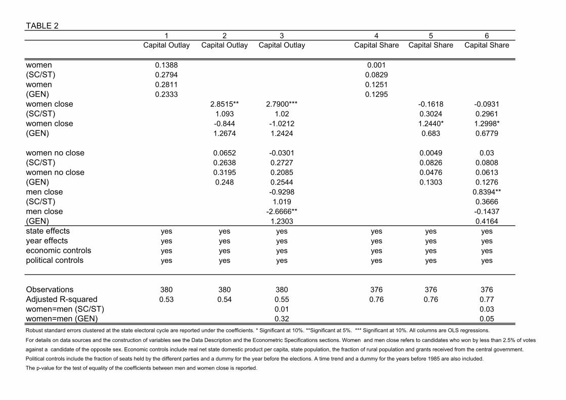
TABLE 21 2 3 4 5 6

Capital Outlay Capital Outlay Capital Outlay Capital Share Capital Share Capital Share

women 0.1388 0.001(SC/ST) 0.2794 0.0829women 0.2811 0.1251(GEN) 0.2333 0.1295women close 2.8515** 2.7900*** -0.1618 -0.0931(SC/ST) 1.093 1.02 0.3024 0.2961women close -0.844 -1.0212 1.2440* 1.2998*(GEN) 1.2674 1.2424 0.683 0.6779

women no close 0.0652 -0.0301 0.0049 0.03(SC/ST) 0.2638 0.2727 0.0826 0.0808women no close 0.3195 0.2085 0.0476 0.0613(GEN) 0.248 0.2544 0.1303 0.1276men close -0.9298 0.8394**(SC/ST) 1.019 0.3666men close -2.6666** -0.1437(GEN) 1.2303 0.4164state effects yes yes yes yes yes yesyear effects yes yes yes yes yes yeseconomic controls yes yes yes yes yes yespolitical controls yes yes yes yes yes yes

Observations 380 380 380 376 376 376Adjusted R-squared 0.53 0.54 0.55 0.76 0.76 0.77women=men (SC/ST) 0.01 0.03women=men (GEN) 0.32 0.05Robust standard errors clustered at the state electoral cycle are reported under the coefficients. * Significant at 10%. **Significant at 5%. *** Significant at 10%. All columns are OLS regressions.





TABLE 3Capital Expenditure 1 2 3 4 5 6

Development Development Development Non-Develop. Non-Develop. Non-Develop.

women 0.4203 -0.00120.286 0.0336

women close 0.3257 0.2927 -0.0188 -0.0191.4715 1.3843 0.1342 0.1348

women no close 0.3712 0.1881 -0.0008 -0.00150.2858 0.3013 0.0318 0.0307

men close -3.6662*** -0.01291.2539 0.095







TABLE 4Capital Expenditure 1 2 3 4 5 6


women 0.108 0.0124(SC/ST) 0.2729 0.0258women 0.3133 -0.0081(GEN) 0.2211 0.0265women close 2.6403** 2.5873*** 0.1182 0.108(SC/ST) 1.0391 0.9687 0.0927 0.0947women close -1.3518 -1.5381 -0.1303 -0.1307(GEN) 1.0974 0.9924 0.1063 0.1061

women no close 0.0403 -0.0592 0.0097 0.0089(SC/ST) 0.2604 0.2697 0.0247 0.0253women no close 0.3802* 0.2628 -0.0007 -0.0003(GEN) 0.2196 0.227 0.0269 0.0257men close -0.8728 -0.0928(SC/ST) 1.0068 0.0592men close -2.8966** 0.0772(GEN) 1.1902 0.1073state effects yes yes yes yes yes yesyear effects yes yes yes yes yes yeseconomic controls yes yes yes yes yes yespolitical controls yes yes yes yes yes yes






TABLE 5Development Exp. 1 2 3 4 5 6(Capital) Social Social Social Economic Economic Economic

women -0.0384 0.9501**0.1376 0.4038

women close -0.4696 -0.472 3.3112* 3.2923*0.5641 0.5649 1.8385 1.875

women no close 0.0025 -0.0105 0.7054* 0.60060.1307 0.1347 0.3652 0.4094

men close -0.2598 -2.09950.3943 1.7275







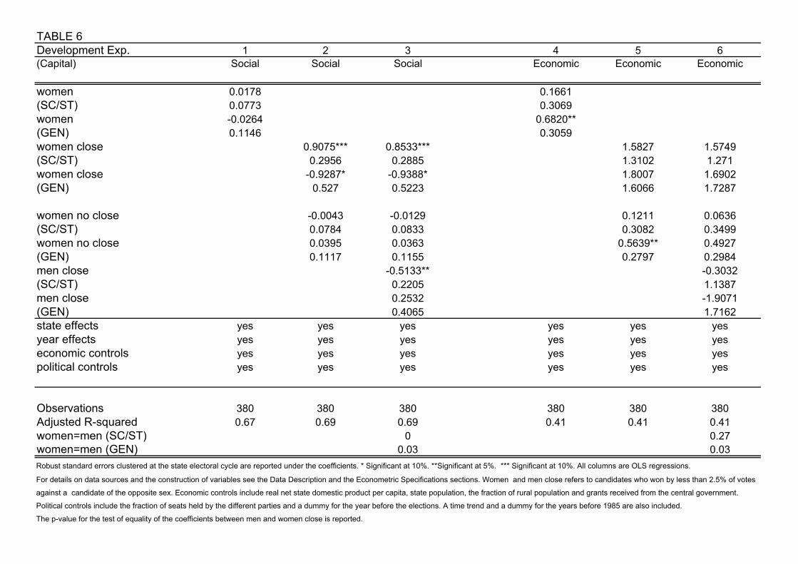
TABLE 6Development Exp. 1 2 3 4 5 6(Capital) Social Social Social Economic Economic Economic

women 0.0178 0.1661(SC/ST) 0.0773 0.3069women -0.0264 0.6820**(GEN) 0.1146 0.3059women close 0.9075*** 0.8533*** 1.5827 1.5749(SC/ST) 0.2956 0.2885 1.3102 1.271women close -0.9287* -0.9388* 1.8007 1.6902(GEN) 0.527 0.5223 1.6066 1.7287

women no close -0.0043 -0.0129 0.1211 0.0636(SC/ST) 0.0784 0.0833 0.3082 0.3499women no close 0.0395 0.0363 0.5639** 0.4927(GEN) 0.1117 0.1155 0.2797 0.2984men close -0.5133** -0.3032(SC/ST) 0.2205 1.1387men close 0.2532 -1.9071(GEN) 0.4065 1.7162state effects yes yes yes yes yes yesyear effects yes yes yes yes yes yeseconomic controls yes yes yes yes yes yespolitical controls yes yes yes yes yes yes

Observations 380 380 380 380 380 380Adjusted R-squared 0.67 0.69 0.69 0.41 0.41 0.41women=men (SC/ST) 0 0.27women=men (GEN) 0.03 0.03Robust standard errors clustered at the state electoral cycle are reported under the coefficients. * Significant at 10%. **Significant at 5%. *** Significant at 10%. All columns are OLS regressions.





TABLE 71 2 3 4 5 6 7 8

Capital Expenditure Economic SocialRoads Bridg. Transp. Comun. Ind. Minerals Energy Irrigation Agriculture Health Water Sup. S.

women close -0.0714 -0.1585 0.146 0.5438 2.3840* 0.6495 -0.4441 0.68160.3278 0.4023 0.2238 1.5173 1.4162 0.647 0.4602 0.5505

women no close 0.1583* 0.2827** -0.0007 0.5563* 0.8939* 0.1317 0.0074 0.01090.0808 0.1324 0.062 0.3199 0.4482 0.1532 0.0812 0.0888

men close 0.1611 0.068 0.0923 -1.3375 -0.6329 -0.9894** -0.1696 -0.5960.3249 0.3859 0.1742 1.1269 1.3544 0.4784 0.2077 0.3806

state effects yes yes yes yes yes yes yes yesyear effects yes yes yes yes yes yes yes yeseconomic controls yes yes yes yes yes yes yes yespolitical controls yes yes yes yes yes yes yes yes

Observations 375 380 376 192 228 378 379 189Adjusted R-squared 0.44 0.3 0.35 0.19 0.59 0.15 0.49 0.76women=men 0.44 0.63 0.85 0.21 0.15 0.03 0.55 0.04Robust standard errors clustered at the state electoral cycle are reported under the coefficients. * Significant at 10%. **Significant at 5%. *** Significant at 10%. All columns are OLS regressions.





TABLE 81 2 3 4 5 6 7 8

Capital Expenditure Economic SocialRoads Bridg. Transp. Comun. Ind. Minerals Energy Irrigation Agriculture Health Water Sup. S.

women close 0.0191 -0.1822 -0.0156 -0.6649 1.6964* 0.1253 0.11 0.3639(SC/ST) 0.1636 0.2293 0.1198 0.8593 0.888 0.3905 0.1908 0.2385

women close -0.1952 -0.1012 0.1667 1.406 -0.1434 0.392 -0.3778 0.3846(GEN) 0.347 0.4034 0.1982 1.3939 1.2379 0.6327 0.4174 0.4782

women no close 0.0001 0.0018 0.0248 0.0138 0.0605 0.011 -0.0187 0.0788(SC/ST) 0.0651 0.0818 0.0338 0.2418 0.2505 0.115 0.0503 0.083women no close 0.1298** 0.2159** -0.0327 0.4640* 0.8808** 0.1412 -0.0119 0.0226(GEN) 0.0612 0.0978 0.05 0.2621 0.3838 0.1062 0.0638 0.0737

men close 0.0116 0.0271 -0.1944* -0.5354 -1.8149* -0.5789** 0.037 -0.2045(SC/ST) 0.16 0.1987 0.1125 0.7491 0.9256 0.2535 0.1696 0.2221men close 0.0997 -0.0166 0.2548 -0.7859 0.8498 -0.4281 -0.2351 -0.317(GEN) 0.324 0.4 0.1615 1.0877 1.3258 0.4499 0.2038 0.3965


Observations 375 380 376 192 228 378 379 189Adjusted R-squared 0.44 0.29 0.35 0.18 0.61 0.14 0.49 0.76women=men (SC/ST) 0.97 0.46 0.24 0.9 0.01 0.09 0.78 0.08women=men (GEN) 0.34 0.85 0.75 0.17 0.43 0.28 0.72 0.27Robust standard errors clustered at the state electoral cycle are reported under the coefficients. * Significant at 10%. **Significant at 5%. *** Significant at 10%. All columns are OLS regressions.





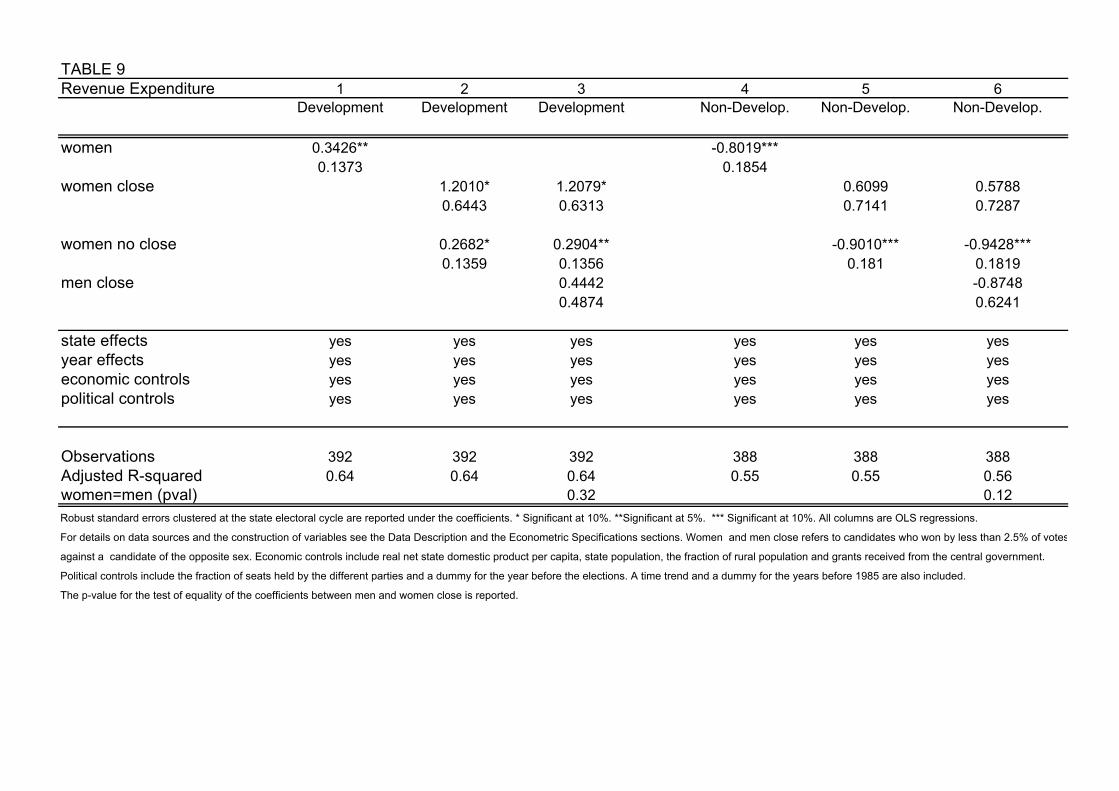
TABLE 9Revenue Expenditure 1 2 3 4 5 6


women 0.3426** -0.8019***0.1373 0.1854

women close 1.2010* 1.2079* 0.6099 0.57880.6443 0.6313 0.7141 0.7287

women no close 0.2682* 0.2904** -0.9010*** -0.9428***0.1359 0.1356 0.181 0.1819

men close 0.4442 -0.87480.4874 0.6241







TABLE 10Revenue Expenditure 1 2 3 4 5 6


women 0.0132 -0.108(SC/ST) 0.1076 0.1344women 0.2602** -0.6384***(GEN) 0.1085 0.1488women close 0.9210** 0.8340** -0.1633 -0.0807(SC/ST) 0.4137 0.4029 0.4112 0.4079women close 0.5096 0.529 0.5516 0.481(GEN) 0.5266 0.5105 0.61 0.6365

women no close -0.012 -0.013 -0.1048 -0.119(SC/ST) 0.1068 0.1062 0.1361 0.1355women no close 0.2371** 0.2526** -0.7071*** -0.7322***(GEN) 0.1135 0.1174 0.1529 0.1601men close -0.7648*** 0.5824**(SC/ST) 0.2753 0.2829men close 1.0313** -1.3238**(GEN) 0.4795 0.6409state effects yes yes yes yes yes yesyear effects yes yes yes yes yes yeseconomic controls yes yes yes yes yes yespolitical controls yes yes yes yes yes yes

Observations 392 392 392 388 388 388Adjusted R-squared 0.64 0.65 0.65 0.55 0.55 0.56women=men (SC/ST) 0 0.12women=men (GEN) 0.42 0.04Robust standard errors clustered at the state electoral cycle are reported under the coefficients. * Significant at 10%. **Significant at 5%. *** Significant at 10%. All columns are OLS regressions.





TABLE 11Development expend. 1 2 3 4 5 6(Revenue account) Economic Economic Economic Social Social Social

women 0.5315*** -0.1670.1744 0.1582

women close 2.4027*** 2.4327*** -1.1507* -1.1643**0.7748 0.7272 0.5995 0.5859

women no close 0.3859** 0.4293*** -0.0956 -0.11520.1491 0.1442 0.1471 0.1476

men close 0.9002** -0.40690.4095 0.3705







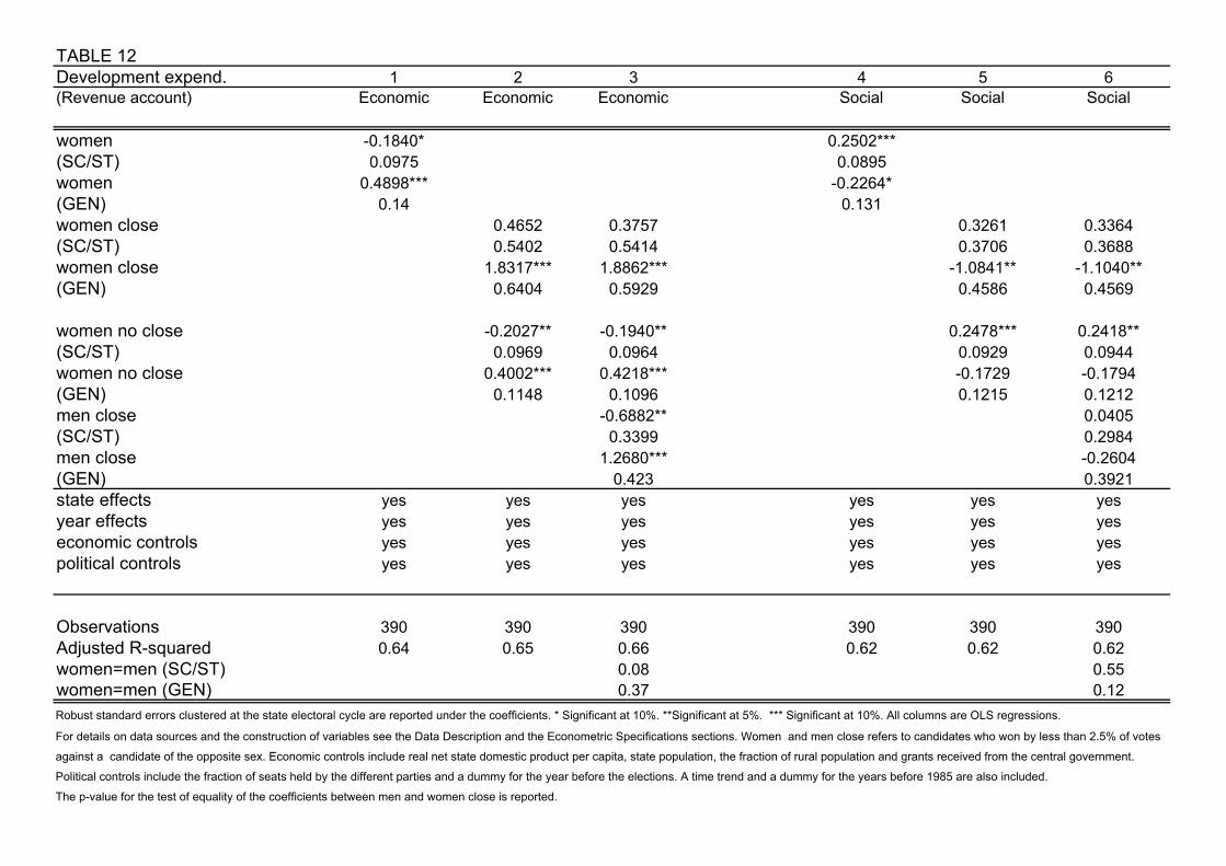
TABLE 12Development expend. 1 2 3 4 5 6(Revenue account) Economic Economic Economic Social Social Social

women -0.1840* 0.2502***(SC/ST) 0.0975 0.0895women 0.4898*** -0.2264*(GEN) 0.14 0.131women close 0.4652 0.3757 0.3261 0.3364(SC/ST) 0.5402 0.5414 0.3706 0.3688women close 1.8317*** 1.8862*** -1.0841** -1.1040**(GEN) 0.6404 0.5929 0.4586 0.4569

women no close -0.2027** -0.1940** 0.2478*** 0.2418**(SC/ST) 0.0969 0.0964 0.0929 0.0944women no close 0.4002*** 0.4218*** -0.1729 -0.1794(GEN) 0.1148 0.1096 0.1215 0.1212men close -0.6882** 0.0405(SC/ST) 0.3399 0.2984men close 1.2680*** -0.2604(GEN) 0.423 0.3921state effects yes yes yes yes yes yesyear effects yes yes yes yes yes yeseconomic controls yes yes yes yes yes yespolitical controls yes yes yes yes yes yes






TABLE 131 2 3 4 5 6 7 8

Revenue Expenditure Social Economic Non-DevEducation Health Water supply Soc. Sec. Welf Agriculture Transport Com. Police State Adm

women close -0.5089 -0.2036 0.1094 -0.9575*** 0.2673 0.4333* -0.4786*** -0.39280.3753 0.1577 0.1813 0.2417 0.4353 0.2606 0.1499 0.3012

women no close -0.0048 -0.0593* 0.0509 -0.0960* 0.3889*** 0.1309* -0.0346 -0.09860.068 0.033 0.0314 0.0517 0.0899 0.0728 0.0237 0.0603

men close -0.2752 -0.0117 0.0054 -0.0618 0.4975 -0.1224 0.2871 0.61990.2408 0.1182 0.0899 0.1709 0.3134 0.196 0.287 0.3744


Observations 390 390 225 371 371 371 368 386Adjusted R-squared 0.74 0.81 0.6 0.52 0.63 0.81 0.71 0.55women=men 0.63 0.26 0.58 0 0.67 0.05 0.05 0.05Robust standard errors clustered at the state electoral cycle are reported under the coefficients. * Significant at 10%. **Significant at 5%. *** Significant at 10%. All columns are OLS regressions. For details on data sources and the construction of variables see the Data Description and the Econometric Specifications sections. Women and men close refers to candidates who won by less than 2.5% of votes against a candidate of the opposite sex. Economic controls include real net state domestic product per capita, state population, the fraction of rural population and grants received from the central government. Political controls include the fraction of seats held by the different parties and a dummy for the year before the elections. A time trend and a dummy for the years before 1985 are also included. The p-value for the test of equality of the coefficients between men and women close is reported.

TABLE 141 2 3 4 5 6 7 8

Revenue Expenditure Social Economic Non-DevEducation Health Water supply Soc. Sec. Welf Agriculture Transport Com. Police State Adm

women close -0.1231 0.0591 0.1193* -0.3044** 0.2762 -0.0308 -0.1151 -0.0558(SC/ST) 0.1932 0.108 0.0672 0.1251 0.3081 0.1261 0.0785 0.1734

women close -0.3102 -0.2195 -0.0215 -0.6967*** -0.0845 0.4249* -0.3312** -0.3303(GEN) 0.3404 0.1405 0.1581 0.219 0.4572 0.237 0.1344 0.2387

women no close 0.0572 0.0011 -0.006 0.0229 -0.069 -0.0194 -0.0091 -0.0613*(SC/ST) 0.0545 0.0263 0.0184 0.0367 0.0557 0.0338 0.0183 0.0349women no close -0.0137 -0.0571** 0.0425 -0.0658 0.3714*** 0.1177** -0.0401* -0.0724(GEN) 0.057 0.0287 0.0255 0.0462 0.072 0.0571 0.0217 0.0491

men close -0.2277 -0.0202 -0.0213 0.1269 0.7623** -0.1796 0.0447 0.0298(SC/ST) 0.1573 0.0864 0.0772 0.1297 0.3821 0.1316 0.0878 0.1611men close -0.0289 -0.0118 0 -0.1144 -0.3869 0.0167 0.217 0.5221(GEN) 0.2562 0.126 0.11 0.1879 0.3665 0.2015 0.2414 0.3458

state effects yes yes yes yes yes yes yes yesyear effects yes yes yes yes yes yes yes yes

yes yes yes yes yes yes yes yespolitical controls yes yes yes yes yes yes yes yes

Observations 390 390 225 371 371 371 368 386Adjusted R-squared 0.74 0.81 0.6 0.52 0.64 0.81 0.71 0.54women=men (SC/ST) 0.68 0.57 0.13 0.01 0.2 0.37 0.19 0.72women=men (GEN) 0.54 0.18 0.9 0.03 0.5 0.15 0.09 0.06Robust standard errors clustered at the state electoral cycle are reported under the coefficients. * Significant at 10%. **Significant at 5%. *** Significant at 10%. All columns are OLS regressions.





TABLE 15Public Goods 1 2 3 4 5 6 7 8

Teacherspc Teacherspc Teacherspc Schools pc Schools pc Schools pc Schools pc Km surf roadsPrimary Middle Secondary Total Primary Middle Secondary (over total)

women close 13.4600* 4.2053 -1.5744 4.7100* 1.0978 1.1083* 0.3751** -7.3709**7.0421 4.4082 2.6892 2.4747 0.9693 0.5656 0.1751 2.973

women no close 0.8482 0.1989 1.8889** 1.7140** 0.5167** -0.0262 -0.0169 2.8469**1.6162 1.2328 0.8658 0.6839 0.2105 0.1024 0.0436 1.082

men close -2.9885 -2.387 -7.8803*** -2.0671 0.1482 -0.3437 -0.2931** 1.11536.074 2.7972 1.6614 2.4397 0.7949 0.3142 0.1411 3.2756


Observations 268 268 268 268 316 316 268 203Adjusted R-squared 0.71 0.95 0.96 0.97 0.98 0.95 0.94 0.9women=men 0.1 0.14 0.02 0.04 0.4 0 0 0.11Robust standard errors clustered at the state electoral cycle are reported under the coefficients. * Significant at 10%. **Significant at 5%. *** Significant at 10%. All columns are OLS regressions.



Political controls include the fraction of seats held by the different parties and a dummy for the year before the elections. A time trend is also included. The p-value for the test of equality of the coefficients

between men and women close is reported.

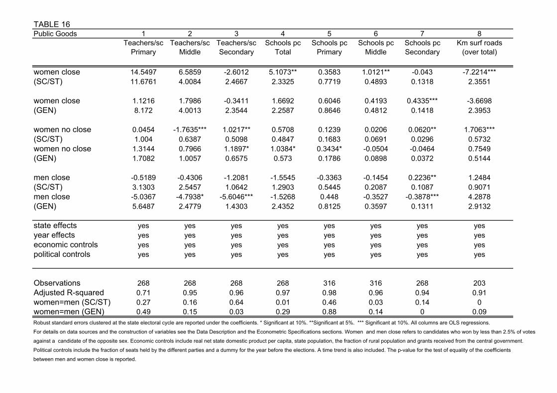
TABLE 16Public Goods 1 2 3 4 5 6 7 8

Teachers/sc Teachers/sc Teachers/sc Schools pc Schools pc Schools pc Schools pc Km surf roadsPrimary Middle Secondary Total Primary Middle Secondary (over total)

women close 14.5497 6.5859 -2.6012 5.1073** 0.3583 1.0121** -0.043 -7.2214***(SC/ST) 11.6761 4.0084 2.4667 2.3325 0.7719 0.4893 0.1318 2.3551

women close 1.1216 1.7986 -0.3411 1.6692 0.6046 0.4193 0.4335*** -3.6698(GEN) 8.172 4.0013 2.3544 2.2587 0.8646 0.4812 0.1418 2.3953

women no close 0.0454 -1.7635*** 1.0217** 0.5708 0.1239 0.0206 0.0620** 1.7063***(SC/ST) 1.004 0.6387 0.5098 0.4847 0.1683 0.0691 0.0296 0.5732women no close 1.3144 0.7966 1.1897* 1.0384* 0.3434* -0.0504 -0.0464 0.7549(GEN) 1.7082 1.0057 0.6575 0.573 0.1786 0.0898 0.0372 0.5144

men close -0.5189 -0.4306 -1.2081 -1.5545 -0.3363 -0.1454 0.2236** 1.2484(SC/ST) 3.1303 2.5457 1.0642 1.2903 0.5445 0.2087 0.1087 0.9071men close -5.0367 -4.7938* -5.6046*** -1.5268 0.448 -0.3527 -0.3878*** 4.2878(GEN) 5.6487 2.4779 1.4303 2.4352 0.8125 0.3597 0.1311 2.9132


Observations 268 268 268 268 316 316 268 203Adjusted R-squared 0.71 0.95 0.96 0.97 0.98 0.96 0.94 0.91women=men (SC/ST) 0.27 0.16 0.64 0.01 0.46 0.03 0.14 0women=men (GEN) 0.49 0.15 0.03 0.29 0.88 0.14 0 0.09Robust standard errors clustered at the state electoral cycle are reported under the coefficients. * Significant at 10%. **Significant at 5%. *** Significant at 10%. All columns are OLS regressions.





TABLE 17Laws 1 2

Land reform HinduSuccession

women close -55.2383*** 4.541914.1678 4.1574

women no close -4.0744 1.73263.1827 1.052

men close 2.4746 -5.5914**8.17 2.2095

state effects yes yesyear effects yes yeseconomic controls yes yespolitical controls yes yes

Observations 356 461Adjusted R-squared 0.92 0.66women=men 0 0.03Robust standard errors clustered at the state electoral cycle are reported under the coefficients. * Significant at 10%. **Significant at 5%. *** Significant at 10%. All columns are OLS regressions.





TABLE 18Laws 1 2

Land reform HinduSuccession

women close -5.8887 9.4976***(SC/ST) 10.1243 3.0797

women close -45.8248*** -1.673(GEN) 10.8614 2.553

women no close -4.4080** 0.3385(SC/ST) 2.1691 0.5335women no close -0.9237 1.6349**(GEN) 2.7136 0.812

men close 10.0988* -2.1982(SC/ST) 5.1059 1.7095men close -11.7342* -4.3767**(GEN) 6.8077 2.0192

state effects yes yesyear effects yes yeseconomic controls yes yespolitical controls yes yes

Observations 356 461Adjusted R-squared 0.92 0.69women=men (SC/ST) 0.18 0women=men (GEN) 0 0.34Robust standard errors clustered at the state electoral cycle are reported under the coefficients. * Significant at 10%. **Significant at 5%. *** Significant at 10%. All columns are OLS regressions. For details on data sources and the construction of variables see the Data Description and the Econometric Specifications sections. Women and men close refers to candidates who won by less than 2.5% of votes against a candidate of the opposite sex. Economic controls include real net state domestic product per capita, state population, the fraction of rural population and grants received from the central government. Political controls include the fraction of seats held by the different parties and a dummy for the year before the elections. A time trend is also included. The p-value for the test of equality of the coefficients between men and women close is reported.

Table A1Descriptive statistics: Variable Obs Mean Std. Dev. Min MaxPop. Growth 544 0.020038 0.006966 -0.01296 0.03102Real NSDP pc 522 0.123431 0.051839 0.045215 0.309966Grants 536 0.426942 0.694855 0.044561 6741605Rural population 560 0.769835 0.080426 0.5614042 0.9252676

women SC/ST 542 0.041435 0.041896 0.0000 0.240741women GEN 542 0.036653 0.027301 0.0000 0.142857women close SC/ST 500 0.002547 0.007434 0.0000 0.044444women close GEN 500 0.003448 0.005699 0.0000 0.02381men close SC/ST 500 0.0033605 0.0091374 0.0000 0.0571429men close GEN 500 0.0034694 0.0068288 0.0000 0.0454545

Congress (prop seats) 544 0.432947 0.259663 0.0000 0.928571Hard Left (prop seats) 544 0.078792 0.148719 0.0000 0.673469Regional (prop seats) 544 0.15039 0.240951 0.0000 0.786325Hindu (prop seats) 544 0.079119 0.130234 0.0000 0.6875Others (prop seats) 544 0.046261 0.083608 0.0000 0.555556Janata (prop seats) 544 0.132581 0.203612 0.0000 0.836735Soft Left (prop seats) 544 0.013527 0.036223 0.0000 0.27044

Table A2REVENUE EXPENDITURE Obs Mean Std. Dev. Min MaxDEVELOPMENT 554 0.6556671 0.0698543 0.3628616 0.7980239

SOCIAL 472 0.3882371 0.0577207 0.1861978 0.6531044

Education 550 0.2140319 0.0432961 0.0854469 0.3773786Health 550 0.0751791 0.0231543 0.0056658 0.1386906Housing 448 0.00486 0.0039723 0.00000717 0.0247883Labour and labour welfare 448 0.0069216 0.0059917 -0.0258231 0.0593069Social Security Welfare 448 0.0291381 0.020329 0.0000 0.1489918Welfare SC/ST 264 0.0212783 0.0172942 0.0000 0.0901957Water supply and sanitation 264 0.0241165 0.0115391 0.0000 0.0594948

ECONOMIC 472 0.2750369 0.0721322 0.001213 0.5307896

General Economic Services 448 0.0160417 0.0201425 0.0003736 0.2661011Agriculture 448 0.1031637 0.0557867 0.0017507 0.5665448Industry and Minerals 447 0.0152988 0.0102186 0.0001165 0.0763455Transport and Comunications 447 0.0405094 0.0318742 -0.0016266 0.1781Water and Power Development 447 0.0994694 0.0678818 -0.3958211 0.368472

NON-DEVELOPMENT 550 0.3294583 0.083895 0.0083134 0.6292282

Organs of the state 466 0.01212 0.0184369 0.0028696 0.4010231State Administration 546 0.1018509 0.0293427 0.0038017 0.2373397Police 446 0.0570928 0.0195838 0.0045695 0.1854423Public Works 447 0.0099368 0.0067125 -0.0127769 0.0477026

Table A3CAPITAL EXPENDITURE Obs Mean Std. Dev. Min MaxDEVELOPMENT 452 0.4529742 0.1590552 -0.4363941 0.8539258

SOCIAL 452 0.0692197 0.0569918 -0.015788 0.4936851

Education 451 0.0087283 0.0088229 0.0000 0.0476581Housing 452 0.0089661 0.0079298 -0.020768 0.0552299Health 451 0.0212459 0.0308545 -0.0586123 0.2350102Welfare SC/ST 258 0.0071205 0.0088164 0.0000 0.0599218Social Sec Welf 344 0.0025188 0.0046127 -0.0142326 0.0365664Water supply and sanit. 257 0.031623 0.0447149 0.0000 0.2105254

ECONOMIC 452 0.3780405 0.1559253 -0.482707 1.209.355

Agriculture 449 0.031976 0.0619198 -0.8110804 0.2610976Industry minerals 447 0.023948 0.0206381 -0.0215158 0.1636151General Economic Serv. 450 0.0151584 0.0241942 -0.0457434 0.2668729Transport Communications 452 0.0673348 0.038521 0.0002859 0.3054822Energy 260 0.0553519 0.0995704 -0.4845973 0.4008722Irrigation 312 0.1913632 0.1098467 0.0006948 0.6373932Roads and Bridges 495 0.0595343 0.0398016 0.0000 0.2496927

NON-DEVELOPMENT 451 0.0135494 0.0137817 -0.0225995 0.1072975

LOANS (repayed/given) 452 0.5341795 0.1635959 0.1238153 1384129

Capital out share 448 0.1155003 0.0554509 -0.0407726 0.3775794Total Disburs. share 448 0.2503434 0.0818953 0.0681453 0.5285614

Table A4Variable Obs Mean Std. Dev. Min Max

Laws

Land reform 430 3.255814 2.616899 0.0000 12Hindu Succession 616 0.1493506 0.3567234 0.0000 1

Public Goods/Education

Teachers pc Primary 326 1.964101 0.7057099 0.6955931 6.617233Teachers pc Middle 326 1.357517 0.7529265 0.2884801 3.41846Teachers pc Secondary 326 1.501463 0.7053546 0.5054514 3.402602

Total Schools pc 326 1.98609 0.6971945 0.7483083 3.571947Primary Schools pc 377 0.7467779 0.3089837 0.221277 1.51994Middle Schools pc 377 0.1927244 0.1126238 0.0428238 0.441846Secondary Schools pc 326 0.0878352 0.03267 0.0352982 0.1658901

Km surf roads/area 257 0.2709579 0.258427 0.0519514 1.381849

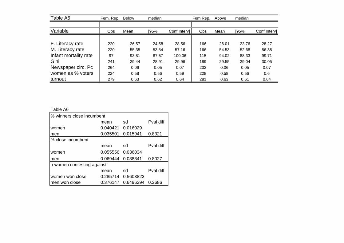
Table A5 Fem. Rep. Below median Fem Rep. Above median

Variable Obs Mean [95% Conf.Interv] Obs Mean [95% Conf.Interv]

F. Literacy rate 220 26.57 24.58 28.56 166 26.01 23.76 28.27M. Literacy rate 220 55.35 53.54 57.16 166 54.53 52.68 56.38Infant mortality rate 97 93.81 87.57 100.06 115 94.02 88.33 99.71Gini 241 29.44 28.91 29.96 189 29.55 29.04 30.05Newspaper circ. Pc 264 0.06 0.05 0.07 232 0.06 0.05 0.07women as % voters 224 0.58 0.56 0.59 228 0.58 0.56 0.6turnout 279 0.63 0.62 0.64 281 0.63 0.61 0.64

Table A6% winners close incumbent

mean sd Pval diffwomen 0.040421 0.016029men 0.035501 0.015941 0.8321% close incumbent

mean sd Pval diffwomen 0.055556 0.036034men 0.069444 0.038341 0.8027n women contesting against

mean sd Pval diffwomen won close 0.285714 0.5603823men won close 0.376147 0.6496294 0.2686

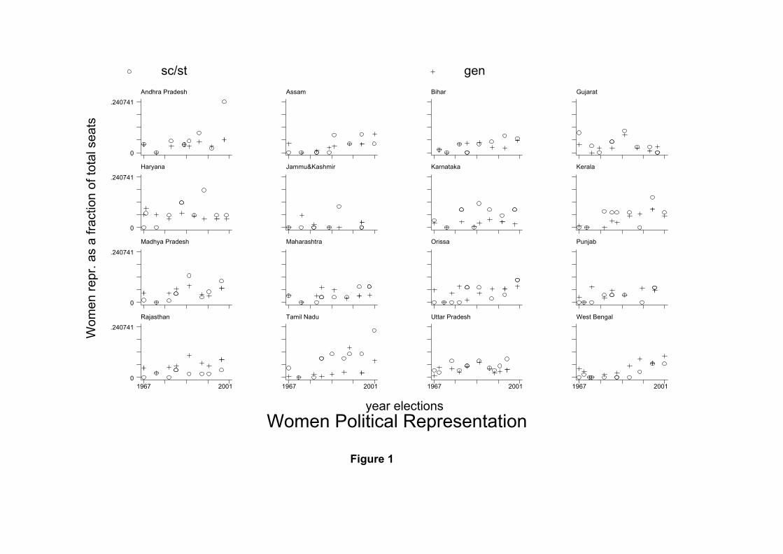
Figure 1

Wom

en re

pr. a

s a

fract

ion

of to

tal s

eats

Women Political Representationyear elections

sc/st genAndhra Pradesh

0

.240741Assam Bihar Gujarat

Haryana

0

.240741Jammu&Kashmir Karnataka Kerala

Madhya Pradesh

0

.240741Maharashtra Orissa Punjab

Rajasthan

1967 20010

.240741Tamil Nadu

1967 2001

Uttar Pradesh

1967 2001

West Bengal

1967 2001

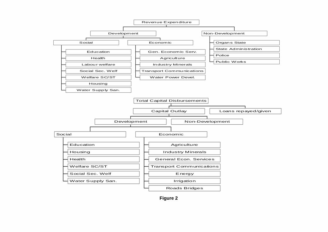
Figure 2

Education

Health

Labour welfare

Social Sec. Welf

Welfare SC/ST

Housing

Water Supply San.

Social

Gen. Economic Serv.

Agriculture

Industry Minerals

Transport Communications

Water Power Devel.

Economic

Development

Organs State

State Administration

Police

Public Works

Non-Development

Revenue Expenditure

Education

Housing

Health

Welfare SC/ST

Social Sec. Welf

Water Supply San.

Social

Agriculture

Industry Minerals

General Econ. Services

Transport Communications

Energy

Irrigation

Roads Bridges

Economic

Development Non-Development

Capital Outlay Loans repayed/given

Total Capital Disbursements

DATA APPENDIX

Electoral data Election Commission of India: Report on State Elections(various issues)

Public Finance data Reserve Bank of India Bulletin (various issues)Population Census of IndiaEducational data Ministry of EducationRoads Reserve Bank of India Report on Currency and Finance

(various issues)Deflator Indian Labor Journal, Indian Labor Gazette, Indian

Labor Journal, Reserve Bank of India Report on Currencyand Finance.

Laws Ministry of Law

22

Women in Politics: Evidence from the Indian states Irma...

Documents

Transcript of Women in Politics: Evidence from the Indian states Irma...