I I

/

• Prestressed Concrete in Transportati'on

.. Systems, p. 14 {;':; ,

~~' • Shear Tests of Concrete Beams Reinforced With Prestressed PIC Tubes, p.68 ,

• Creep and Shrinkage Characterization for Anal zin Prestressed C6ncrete

, ","'

~ Reflections on the Beginnings of . Prestre$sed Concrete in America­

Part 9 (cont.): The End of the "Beginnings," p, 123 -"'-' .

• Hollow-Core Slabs for 6eachHouse Condominiums,p.15.8 +

• Reader Comments on Dapped-End

~ Creep and Shrinkage ••• .!. Characterization for .:. ~: Analyzing Prestressed i Concrete Structures

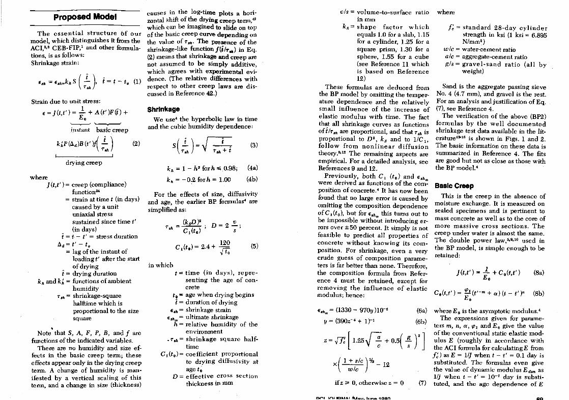
Zdenek p, Belent Prole""" 01 c,..u Engl.-rt"ll Notthw.stern UrivefSIty E._on, lltinoi.

Lilsa Panula' E!¥I1"r, TAMS (11w-tts.

AOb9\t, McCorIIly and StratlOO) Now York, NY

De formation, d ~e to creep .nd shrin k-\/<, a rt< no rmally se,'cral

time. largcT than "last", derom,a'ions in concre te st ruc'm e" ~' Tcq"entl}' , the.e ddonna'ion. C~\l.<e e'Oe"ive crocking and deflection, or po"ible f.ilu", with on inhere", 10 « iTI Ser­,'keabiH'y, d llnbili' )' and lon g_tim~ •• fel}' o f cOncrete ,,,uctme., Thus, tM'" is an " rgen t oe~d for a reliahle method 10 predict creep and ,hrink­age, e. ped.lly for slen<ler pre.tre, ,,,d concrete .truc'ure •.

lIe<,,,,t lr, we ha,-e witne,sed cflOrt. 10 in troduce creep and , h rinkage i"to des,sn ",comme"d "hon"'~' "~ d 10 ,Ievel" p ",on' ",.lidic pred iction for­",,,I,.' O '-er 'he la,t decade, how­evOf, the subj<"Ct ha, he~" pl.g"ed b)' persi,ten t disog"",ment as to who, i, the pruper and 01~i", .1 fonnub'ioll to

he u>e<1.'" ,~ltbouih ..,,~ral ""rt;,,,,o' conciu,;ons ha\'~ bee" drawn from theoretic.l arguments,~' we .hall d~­liLcra,d)' lea,,, them o"t_ The mo,t ",Ie"",, , .nd co"';nc;,\~ a'8,,,neot i" of course, ,he o x""fiIn<,n'al e,;denre a"d how we ll the rl.ta conelat~ with 'he ""toal behadof of e,isting ,truc­tu"" ,

Although this l,as not he.,,, gene .. all)' ",a!ired, vast e.pe,;m~"t.1 in!Qr­malion on creep and ,hrinkoic has ai_ ",ady he"n ."c"m"lat~ d ill the Ii'~r­ature,' UnfOrtunatelr, ,h~ provi,ions of a recert' international model cod~ were ,,,pported by ,."t')- lim itcd com­pa,;",,,, w ith test d",. , ,elec'~rl >omewlw . rbi' ..... 'I)' , This wa. onJer-

'F.,,,, • .t,, C"d u'" Rooo,,.h "";"'"', ~"",,,, .• ,",,,, Un.""""" E,-__ , "hoo;~

standable in vie w of ,he Icdio",ne .. of ",,' da ... flUing whe" penorrncd in the tradition.l way_hy hand, Re­cemly, however, hi~hl}' effect i-'e computer optimization method. for analyzinK and fluing te.t data ha"e I:>e~n de'-eloped" and, at 'hc 'ame time, ,he a,-&ilable 'e" da'a from ,-ori­ou. labo",'orio. ha,,, bee" c-oll""red and organized'

Thi. enabled de,-eiopmc,,' of a n,'w pr<.>diction modcl ill Re ference ~ w hich wc will call the BY model Compared to other e xhting mod­cls,"~' thi' One ~h-e ... far superior o,·c.all a2.eement witl, the hulk of a,-a.ilable test data' (S-I di/Tcn>nt data "'IS), Th~ coeffiden' of variation of ,he eree p prediction i, a, low ... 8 '0 12 pe""'''t when the e l."", mooulu, Or one .hrinkaKe ,-all1e i. knowo , ."d obout 16 to 24 pe",..,nt when it i. " n_ k""w".

To attain good accu~"'-'v, th~ earlier SP mooel' ""luire. that not onl)· the s're"!(Ih bu, al.., se'"ral compo.ition (mix) paramcters of cone're'e bc known, Bran",n', (ACI 2 09)'0' model i. ,im ilarly based, On the other h"nd, the inp"t for 'he CEB-F I P Model Code fonnul.tiOll' i, more limited, <e'lui rin!l ooly ,he streng!h and the type of ""m~nt, .nd po"ibly tho ela,­tio modulus of conCTe te_ I'OT p",limi­nary de';gn, ;11 w hich the c'Ompos ihon of the concrete to loc u>cd might not ret be known, 'TId al.., for thc des ign of ordinary structure" i, i. desirable '0 hal'e a ,impler mode l thaI ""luire, os few material char""t",;" ie. a> po,,;_ bl~, preferably jmt tbe 'trcn~h, wh ile mainta;"ing at th" ,ame ' i,ne •• ulli­c';""t ac'''''ac'v_ D~,-elopment of ""ch a model.

whkh "'~ will e.n BP2, i. our main objectil" _ Thi, model will "'p",,,, n' a 'implified ' ·e"ion of the carlie r BP model:' hen~e, 'he b.o<; kgm,,,,d dis­cussionS'·" TIeed no' he repeat",L Althou~h an ",-'~ur.te p",di~'ion of C""'p and .hT;"kage i, needed mainly

Synopsis Many p' &stressed conC reto

structures a,e sensitive ttl otMP and sM nkage, neoessitating accufate predi<:lOon. Cr .... p aM shrinkage charactorization, and mod~9 10< p'ed lctl ng its pa rameters , aTe analyzed, Md a new s;mplified model is propo~.

Extensiv<o g raphical and stati$!~ cal comparisons with test data available ln tOO literature a", made lD verify a nd calibrate !he model Th e deviatio~ s of predlotiOns mada using " xlsting ACI and CEe models lrom the same data are aoo determined, The coeHicieF\!s of variation and 95 petoel1t confi­dence limits of tM oov;"tioM from toS! data ara evaluated, I\;s fou.nd that the proposed model is more re presclllatll'e 01 actual COtlditIons than p<evioos metl>ods,

Impr ov a ments of prediction when measurements 01 abort-time delormet"" are availabto a,,, also discussed, Finally, a detailed practical example 01 a segmental

box ""de< bridge is given.

for prest"" .. d " ruclures, !hc m",le l can of co ," .. e be u""d for .1I ,,-,,,c rete _<t ructu",.,

To edimate Ihe error in material de­« ',ipti"n , we adopt a. OUT wco nd ob_ ject;'.., " >tati,tical .nol y,;' of the de­vialions fro", tCst dat. _ At the , arne 'ime, we will com pare ' he data fit. for the preoe nt model with those or Bran­>on', (ACI) modol~' and t f,., CE B- FlP ,\Iodel Codc' In th~ proc,, " these two will be al,", <-o"'pared mutu"II}·; 'hi' ha, not be" n done previousl)" in 'pite of m"oh ,Ii..,,,,,ion_ For. com­pariwn of the """ ';om BP model w it h tM , arne altd ,uan)' further te , t d,,"~ Rdi::n>"cc 4 m~)' he con.u lteJ,

Proposed Model

The essential structure bf our model, which distinguishes it from the ACI,2,3 CEB-FIP,l and other formula­tions, is as follows: Shrinkage strain:

Strain due to unit stress:

E = J (t,t' ) = 1.. + A (t')F (i) + Eo

'---.-' \ . instant basic creep

k~P(t:.d)B(t,}J i) (2) ~\ 'T,,,

drying creep

where J (t,t') = creep (compliance)

function34

= strain at time t (in days) caused by a unit uniaxial stress sustained since time t' (in days)

i = t - t' = stress duration t:.d = t' - to

= lag of the instant of loading t' after the start of drying

t = drying duration k" and k~ = functions of ambient

humidity

,

T ," = shrinkage-square halftime which is proportional to the size square

Note that S, A, F, P, B, and f are functions of the indicated variables.

There are no humidity and size ef­fects in the basic creep term; these effects appear only in the drying creep term. A change of humidity is man­ifested by a vertical scaling of this term, and a change in size (thickness)

causes in the log-time plots a hori­zontal shift of the drying creep term,42 which can be imagined to slide on top of the basic creep eurve depending on the value of T,,,. The presence of the shrinkage-like functionf(ilT·",) in Eq. (2) means that shrinkage and creep are not assumed to be simply additive, which agrees with experimental evi­dence. (The relative differences with respect to other creep laws are dis­cussed in Reference 42.)

Shrinkage We use4 the hyperbolic law in time

and the cubic humidity dependence:

( t)~ t S - = --T,II T,,,+t

k" = 1 - h3 forh ... 0.98;

k" = -0:2 forh = 1.00

(3)

(4a)

(4b)

For the effects of size, diffusivity and age, the earlier BP. formulas4 are simplified as:

(k sD)2 D = 2 .£.; T,,, ;= C

1(t

O) ; s

in which

120 C 1(t O) = 2.4 + rT

v to (5)

t = time (in days), repre­senting the age of con­crete

to = age when drying begins t = duration of drying

E,,, = shrinkage strain E,,, = ultimate shrinkage

h = relative humidity of the environment

. T." = shrinkage square half­time

C 1 (to) = coefficient Proportional to drying diffusivity at age t~

D = effective cross section thickness in mm

vIs = volume-to-surface ratio inmm

ks = shape factor which equals 1.0 for a slab, 1.15 for a cylinder, 1.25 for a square prism, 1.30 for a sphere, 1.55 for a cube (see Reference 11 which is based on Reference 12)

These formulas are deduced from the BP model by omitting the temper­ature dependence and the relatively small influence of the increase of elastic modulus with time. The fact that all shrinkage curves as functions of i IT ," are proportional, and that 'T ," is proportional to D2, ks and to lIC 1>

follow from nonlinear diffusion theory.9,12 The remaining aspects are empirical. For a detailed analysis, see References 9 and 12.

Previously, both C 1 (to) and E,,, were derived as functions of the com': position of concrete.4 It has now been found that no large error is caused by omitting the composition dependence of C 1 (to), but for E,,, this turns out to be impossible witho~t introducing er­rors over ±50 percent. It simply is not feasible to predict all properties of concrete without knowing its com­position. For shrinkage, even a very crude guess of composition parame­ters is far better than none. Therefore, the composition formula from Refer­ence 4 must be retained, except for removing the influence of elastic modulus; hence:

E."", = (1330 - 970y)10-6 (6a)

y = (390z-4 + 1)"-1 (6b)

z = ~ [ 1.25 {1 + 0.5( ; r] x( 1 + sle ) 1fa - 12

wle

if z ;;;. 0, otherwise z = 0 (7)

DI""I 11'\1 IDMAr , .... G,,_ 111r'l.a i OCln

where

f~ = standard 28-day cylinder strength in ksi (1 ksi = 6.895 N/mm2 )

wle = water-cement ratio ale = aggregate-cement ratio gls = gravel-sand ratio (all by

weight)

Sand is the aggregate passing sieve No.4 (4.7 mm), and gravel is the rest. For an analysis and justification of Eq. (7), see Reference 4.

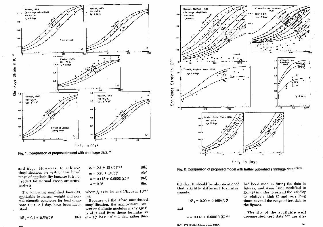
The verification of the above (BP2) formulas by the well documented shrinkage test data available in the lit­eraturel3016 is shown in Figs. 1 and 2. The basic information on these data is summarized in Reference 4. "The fits are good but not as close as those with the BP model. 4

Basic Creep This is the creep in the absence of

moisture exchange. It is measured on sealed specimens and is pertinent to mass concrete as well as to the core of more massive cross sections. The creep under water is almost the same. The double power law,5,9,10 used in the BP model, is simple enough to be retained:

J(t,t') = .1... + Co(t,t') (8a) Eo

C o(t,t') = ~: (t'-m + 0:) (t - t')n (8b)

where Eo is the asymptotic modulus.4

The expressions given for parame­ters m, n, 0:, IPl and Eo give the value of the conventional static elastic mod­ulus E (roughly in accordance with the ACI formula for calculatingE from f~ ) as E = lIJ when t - t' = 0.1 day is substituted. The fonnulas even give the value of dynamic modulus E dl/7l as 1/J when t - t' = 10-7 day is substi­tuted, and the age dependence of E

If) I

0

.E c c ... -en \I) CI C ~ C ... .r:. en

Keelon. 1965

1.0 (Shrinkoge - simplified 1 RH =20% to := 8 days

0.8

0.6

0.4

0.2

1.2 Keelon. 1965

RH =20% 1.0 Cyl. 3". gil

0.8

0.6

0.4

0.2

Siu eflecl

100 0.8

Keelon. 1965 RH =75%

0.6 to I: edays

0.4

E flecl of various curino days

100

(d)

(a)

Keelon.1965 RH =50% 10= B days

Keelon. 1965 RH =50%

1.0 Cyl. 3"x g"

0.8

0.6

0.4

0.2

(c)

1000

10

t-t o in days

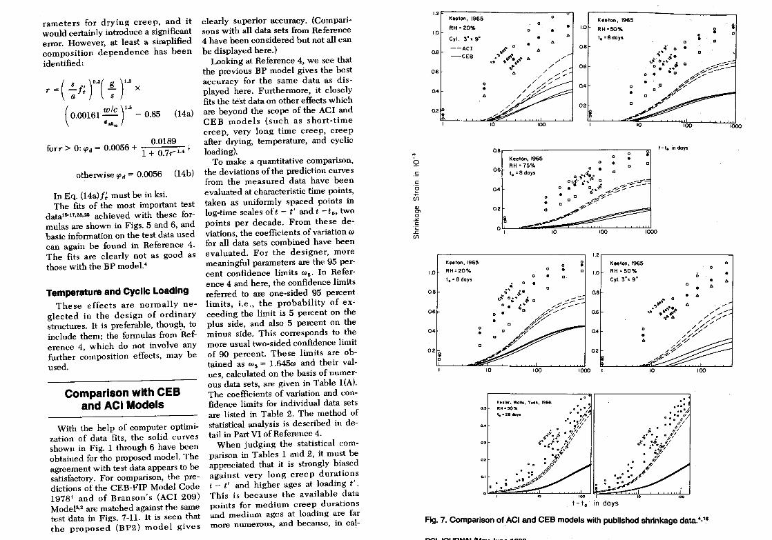
Fig. 1. Comparison of proposed model with shrinkage data. 16

and Edlin' However, to achieve simplification, we restrict this broad range of applicability because it is not needed for normal creep structural analysis.

• The following simplified formulas,

applicable to normal weight and nor­mal strength concretes for load dura­tions t - t' .,. 1 day, have been iden­tified:

IIEo = 0.1 + 0.5/(f'~)2 (9a)

'Pl = 0.3 + 15 (f'~ )-1.2 (9b)

m = 0.28 + I1(f'~)2 (9c)

n = 0.115 + 0.0002 (f'~ )3 (9d)

ex = 0.05 (ge)

where f~ is in ksi and IIEo is in 10-6/

psi. Because of the afore-mentioned

simplification, the approximate con­ventional elastic modulus at any age t' is obtained from these formulas as E = I1J for t - t' = 1 day, rather than

t - to in days

Fig. 2. Comparison of proposed model with further published shrinkage data.4,13-15

0.1 day. It should be also mentioned that slightly different formulas, namely:

IIEo = 0.09 + 0.465/(f':)2

and

n = 0.115 + 0.00013 (f': )3.4

had been used in fitting the data in figures, and were later modified to Eq. (9) in order to extend the validity to relatively high n and very long times beyond the range of test data in the figures.

The fits of the available well documented test datal7,26 are dis-

....

If)

a. "-

CD

b C

J

O.~O 04'

A'! L' Hermite, Mamillan, Lefevre. 1965.1975 (sealed) 4' Canyon Ferry Dam. 1958, A

0.7 sealed A 0.4' (Basic creep - simplified)

t::.t::. .,,60"-' t::. \,.

0.40 0.6

0.3' 0.'

0.30

0.2~

0.20 D

0.2 0

o.le e

A

0.10 0.01 1.0 0

0 .. Ross Dam. 1953,1958. sealed

1.8 Dwarshak Dam. 1968, sealed JqI/'

000 0.9 0

0

00

1.6 0.8 tl~i" .. ' 0" .1-

, .' , ,/ 0.7

1.4 0 0

000 0

0 0.6

1.2 ~(J\" • 0

, .'!> # 0.' , 1.0 0

00

0 0.4

0 .•

0.3

0.6

100

0.4 Shasta Dam, 1953. 1958. sealed

0.6

00 0

0., 00·

0.30 York, Kennedy. Perry. 1970, sealed 60

"-'

00/ 0

,.'l.6

0 0..,

0.' 0.20

0.2

o.le 0.1 1.0 10 100 10 100 1000

t - t' in days

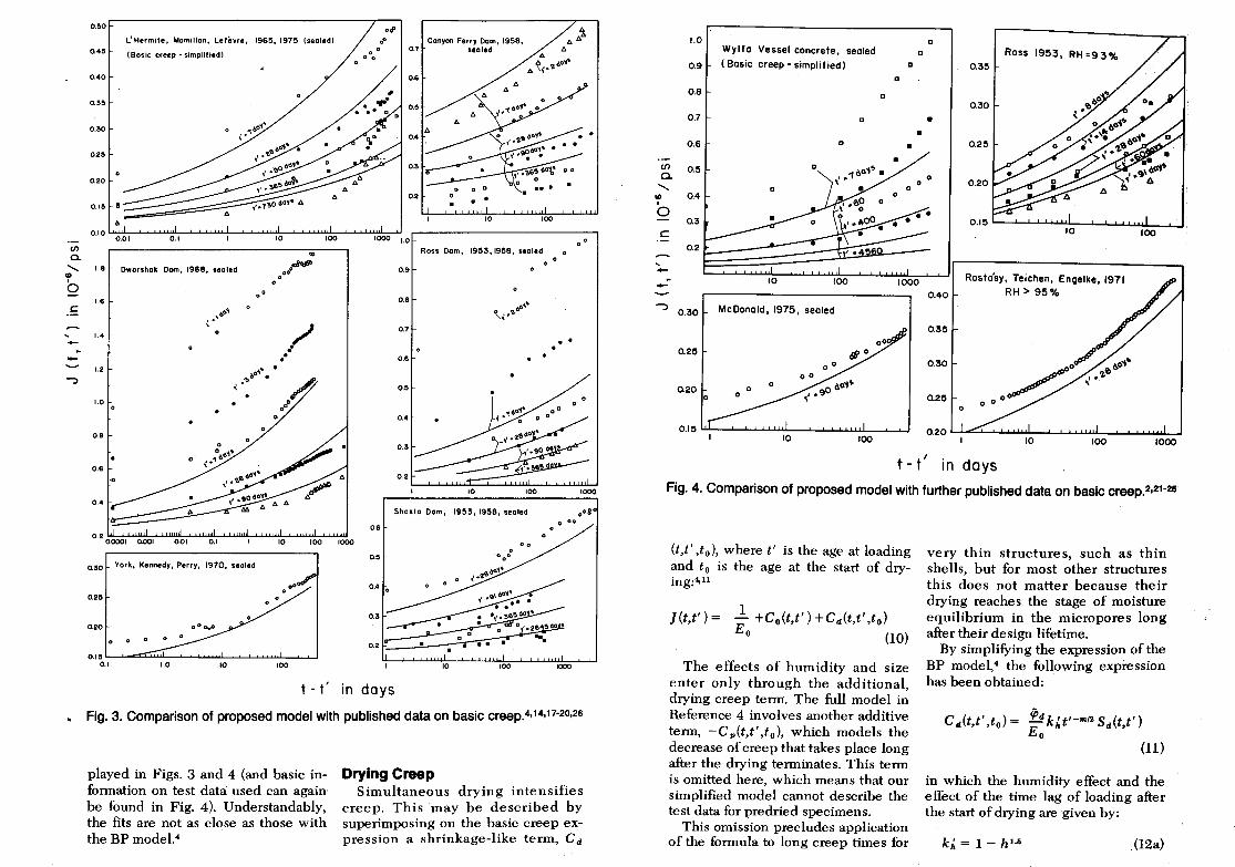
Fig. 3. Comparison of proposed model with published data on basic creep.4,14,17-20,26

played in Figs. 3 and 4 (and basic in­formation on test data used can again' be found in Fig. 4). Understandably, the fits are not as close as those with the BP mode1.4

Drying Creep Simultaneous drying intensifies

creep. This may be described by superimposing on the basic creep ex­pression a shrinkage-like term, Cd

1.0

0.9

O.B

0.7

0.6

(J) 0.5 a. "-

CD 0.4 I

0 0.3 C

0.2 , --J 0.30

0.25

0.20 0

0.15

Wylfa Vessel concrete, sealed

(Basic creep - simplified) D

D

D

D

D •

McDonald, 1975, sealed

0

D

D

• •

Ross 1953, RH=93% 0.35

030

0.25

0.20

0.15

Rosta'sy, Teichen, Engelke, 1971 RH> 95%

t - t' in days

Fig. 4. Comparison of proposed model with further published data on basic creep.2,21-25

(t,t' ,to), where t' is the age at loading and to is the age at the start of dry­ing:4,ll

] (t,t') =

The effects of humidity and size enter only through the additional, drying creep term. The full model in Reference 4 involves another additive term, -C p(t,t' ,to), which models the decrease of creep that takes place long after the drying terminates. This term is omitted here, which means that our simplified model cannot describe the test data for predried specimens.

This omission precludes application of the formula to long creep times for

very thin structures, such as thin shells, but for most other structures this does not matter because their drying reaches the stage of moisture equilibrium in the micropores long after their design lifetime.

By simplifYing the expression of the BP model,4 the following expression has been obtained:

ipd k ' t'-m12 S (t t' ) Eo " d ,

(11)

in which the humidity effect and the effect of the time lag of loading after the start of drying are given by:

k~ = 1 - h 1•5 . (12a)

I/)

0-....... ... I

0

c:

, --....,

1.0

0.8

0.6

0.4

0.2

1.8

1.0

o.e

L" Hermite, Mamillan I Lefevre I 1965. 1971

(Drying creep - simplified)

RH' !l0"4

0.01 0.1

Troxell • Raphael, Dovil, 19!18

0.8 Meye .. and Moily. 1970

RH-!lO"4

0.7

0.6

o.e

0.4

. '" .

0.'

04

0.3

02

t - t'

0.6...--------------71

Hummelelol.1962 RH'6!1"4

0.!5 0°

/P.... • ,.1.6 0 :

0.4 •• _,,'" ,

0.3

1.0

0.8

0.6

10 100

l' Hermite I Mamillan I 1965

0.6

0.4

0.3

Lamboue. Mommenl, 1976

Concrete p26. p29

!

Rasla.y. 1971 RH-6!1"4

0.1 10 100

in days

1000

1000

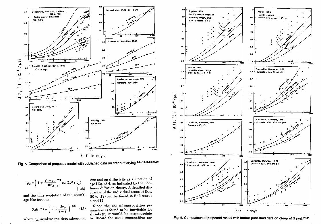
Fig. 5. Comparison of proposed model with published data on creep at drying.4,14,15,17,24,28,29

( t' - t )-1 ~d = 1 + H}r'1I

6 fPd (10

6 E.II.)

(12b)

and the time evolution of the shrink­age-like tenn is:

( 3T )-6.35

Sd(t,t')= 1 +~ t - t

(13)

where 7'.11 involves the dependence on

size and on diffusivity as a function of age [Eq. (5)], as indicated by the non­linear diffusion theory. A detailed dis­cussion of the individual tenns ofEqs. (9) to (13) can be found in References 4 and 11.

Since the use of composition pa­rameters is found to be inevitable for shrinkage, it would be inappropriate to discard the same composition pa-

1.0

0.9

o.a

0.7

0.6

0.' . 0.4

0.3

0.9

0.8

0.7

cJ) 0.6

a. .......

III a.' I

Q 0.4 e

c:

0..3

.-0.6

J 0.'

0.4

0.3

0.2

0.7

0.,

0.4

03

0.2

k._~ton. 1965

(Dry-ing cr •• p - simplified)

Humidity effeci. smoll

Size cylinder. 3-. g-

ke.ton. 1965 Humidity effect, large Sire cylinders 6".IS It

Lombo"" Mommen., 1976 Coner.t. p50, p51

Lambotte. Mommens, 1976

Concrete p2. p52 and p54

1000

0.8

0.7

0.6

0'

0.4

03

0.4

0..3

Lambotte. Mommens, 1976 0.6 Concrete p34, p35 and p49

0.'

0..4

0.3

Lambotte, Mommen., 1976 Concrete p23. p40 and p41

t - t' in days

+

a

1000

..

Fig. 6. Comparison of proposed model with further published data on creep at drying.16,27

rameters for drying creep, and it would certainly introduce a significant error. However, at least a simplified composition dependence has been identified:

_ ( s , )O.3( g )1.3 r - -Ie - X

a s

(0.00161 w1C)1.5 _ 0.85

E·"oo (14a)

0.0189 forr> 0: I{)tJ = 0.0056 + -.:......:..::...:...;-

1 + 0.7r-1.4 '

otherwise I{)tJ = 0.0056 (14b)

In Eq. (l4a)I~ must be in ksi. The fits of the most important test

dataliH7,23,25 achieved with these for­mulas are shown in Figs. 5 and 6, and basic information on the test data used can again be found in Reference 4. The fits are clearly not as good as those with the BP model. 4

Temperature and Cyclic Loading These effects are normally ne­

glected in the design of ordinary structures. It is preferable, though, to include them; the formulas from ·Ref­erence 4, which do not involve any further composition effects, may be used.

Comparison with CEB and ACI Models

With the help of computer optimi­zation of data fits, the solid curves shown in Fig. 1 through 6 have been obtained for the proposed model. The agreement with test data appears to be satismctory. For comparison, the pre­dictions of the CEB-FIP Model Code 19781 and of Branson's (ACI 209) Model3,2 are matched against the same test data in Figs. 7-11. It is seen that the proposed (BP2) model gives

clearly superior accuracy. (Compari­sons with all data sets from Reference 4 have been considered but not all can be displayed here.)

Looking at Reference 4, we see that the previous BP model gives the best accuracy for the same data as dis­played here. Furthermore, it closely fits the te·st data on other effects which are beyond the scope of the ACI and CEB models (such as short-time creep, very long time creep, creep after drying, temperature, and cyclic loading).

To make a quantitative comparison, the deviations of the prediction curves from the measured data have been evaluated at characteristic time points, taken as uniformly spaced points in log-time scales oft - t' and t -to, two points per decade. From these de­viations, the coefficients of variation 00

for all data sets combined have been evaluated. For the designer, more meaningful parameters are the 95 per­cent confidence limits 00 5 • In Refer­ence 4 and here, the confidence limits referred to are one-sided 95 percent limits, i.e., the probability of ex­ceeding the limit is 5 percent on the plus side, and also 5 percent on the minus side. This corresponds to the more usual two-sided confidence limit of 90 percent. These limits are ob­tained as 005 = 1.64500 and their val­ues, calculated on the basis of numer­ous data sets, are given in Table l(A). The coefficients of variation and con­fidence limits for individual data sets are listed in Table 2. The method of statistical analysis is described in de­tail in Part VI of Reference 4.

When judging the statistical com­parison in Tables 1 and 2, it must be appreciated that it is strongly biased against very long creep durations t - t' and higher ages at loading t'. This is because the available data points for medium creep durations and medium ages at loading are far more numerous, and because, in cal-

., o

1.2r-------.,..---------..-.

1.0.

0..8

0..6

Keelon. 1965

RH = 20.%

Cyl. 3", 9"

--ACI

-CEB

Keelon. 1965

o •

1.0. RH=2o.%

I. =8 days

0..8

0.'

0.4

0.0

.. ,

o o

•

0

• D

106

Kesler, Wallo, Yuan. 1966. RH-5C)'t.

t.· 28 day.

o o I

o

• K e. Ion. 1965

• 1.0. RH=50% A

I. =8doy.

0..8

o.S

0.4 0

• 0.2 D

i D

10.

1.2 0 Keelon. 1965 0 • • D RH·5o.% 1.0.

D Cyl. 3". g"

0.8

00

10

1-10 in do.ys

0 • 0 .; • 0 ++ 0

="0'" ;-t-: o.~ .. 0 • ++

0 • ·0

• .0

100

t-to in days

" 0 • • '"

'00

Fig. 7. Comparison of ACI and CEB models with published shrinkage data.4,18

__ I ."" ......... 1&1 ... ___ 1 ____ ... __ _

a & D

0

"

1000

0 0

• • A

'"

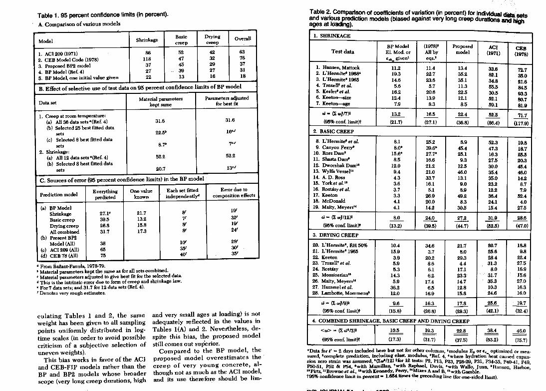
Table 1. 95 percent confidenC$ limits (in percent).

A. Comparison of various models

Model Shrinkage Basic Drying Overall creep creep

1. ACI209 (1971) 86 52 42 63

2. CEB Model Code (1978) 118 47 32 76

3. Proposed BP2 model 37 45 29 37

4. BP Model (Re£. 4) 27 -- 39 27 31

5. BP Model, one initial value given 22 13 16 18

B. Effect of selective use of test data on 95 percent confidence limits of BP model

Material parameters Parameters adjusted for best frt Dataset kept same

1. Creep at room temperature: (a) All 36 data sets • (Ref. 4) 31.6 31.6

(b) Selected 25 best fitted data sets 22.5& 16eJ

(c) Selected 8 best fitted data sets 8.7" 7eJ

2. Shrinkage: (a) All 12 data sets • (Ref. 4) 52.2 52.2

(b) Selected 8 best fitted data sets 20.7 13eJ

C. Sources of error (95 percent confidence limits) in the BP model

Prediction model Everything One value Each set fitted Error due to

predicted known independently" composition effects

{a) BPModel Shrinkage 27.1" 21.7 8' 19'

Basic creep 39.5 13.2 7' 32'

Drying creep 26.8 15.8 8' 19'

All combined 31.7 17.3 8' 24'

(b) Present BP2 Model (All) 38 10' 28'

(c) ACI 209 (All) 65 35' 30'

(d) CEB 78 (All) 75 40' 35'

_.-• From Bdant-Panula, 1978-79. & Material parameters kept the same as for all sets combined. e Material parameters adjusted to give best fit for the selected data. 4 This is the intrinsic error due to form of creep and shrinkage law. " For 7 data sets; and 31. 7 for 12 dat~ sets (Ref. 4). 'Denotes very rough estimates.

culating Tables 1 and 2, the same weight has been given to all sampling points uniformly distributed in log­time scales (in order to avoid possible criticism of a subjective selection of uneven weights).

This bias works in favor of the ACI and CEB-FIP models rather than the BP and BP2 models whose broader scope (very long creep durations, high

and very small ages at loading) is not adequately reflected in the values in Tables l(A) and 2. Nevertheless, de­spite this bias, the proposed model still comes out suPerior.

Compared to the BP model, the proposed model overestimates the creep of very young concrete, al­though not as much as the ACI model, and its use therefure should be lim-

Table 2: Comparison of coefficients of variation (in percent) for Individual d8ta and vanolJs prediction models (biased against very long creep durations and high88ts ages at lOading).

1. SHRINKAGE

BPModel (1978)' Proposed ACI CEB Test data El. Mod. or Alloy model (1971) (1978)

EM. givenl eqs.·

1. Hansen, Mattock 11.2 11.4 13.4 33.6 72.7 2. L'Hermite' 1968' 19.3 22.7 35.2 82.1 35.0 3. L'Hermite" 1965 14.6 23.6 35.1 34.8 21.6 4. Troxell' et al. 5.6 5.7 11.3 55.5 84.5 5. Kesler" et al. 16.2 20.6 22.5 30.5 93.3 6. Keeton--slze 12.4 13.9 12.1 52.1 80.7 7. Keeton---ege 7.9 8.3 8.5 59.1 81.9

tJ (I "'In>' 13.2 16.5 22.4 52.5 71.7

(95% coni limit)t (21.7) (27.1) (36.8) (86.4) (117.9)

2. BASIC CREEP

8. L'Hermite' et al. 8.1 25.2 8.9 52.3 19.8 9. Canyon Ferry" 8.0* 39.6* 45.4 47.3 18.7

10. Ross Dam" 15.6* 27.7* 25.1 16.3 25.5 11. Shasta Dam' 8.5 16.6 9.3 27.5 20.3 12. Dworshak Dam" 12.0 21.2 12.5 30.0 45.4 13. Wylfa Vessel" 9.4 21.0 46.0 35.4 46.0 14. A. D. Ross 4.3 33.7 13.1 35.0 14.2 15. Yorket al. u 3.6 16.1 9.0 23.2 8.7 16. Rosblsyet al. 3.7 5.1 8.9 12.2 7.9 17. Keeton 3.3 26.9 49.2 36.4 52.4 18. McDonald 4.1 20.0 8.3 24.1 4.0 19. Maity, Meyers" 4.1 14.2 30.5 15.4 27.5

tJ - (I "'1112)1 8.0 24.0 27.2 31.9 28.6

(95% con£. limit)t (13.2) (39.5) (44.7) (52.5) (47.0)

3. DRYING CREEP

20. L'Hermite", RH 50% 10.4 34.6 21.7 20.7 18.8 21. L'Hermite" 1965 15.9 3.7 8.0 25.6 9.8

22. Keeton 3.9 20.2 29.3 28.4 22.4 23. Troxell' et al . 5.9 8.6 4.4 31.3 27.5 24. Rosblsy 5.3 6.1 17.1 8.0 16.9

25. Mossiossianu 14.3 6.2 23.3 - 31.7 15.6

26. Maity, Meyers" 5.9 17.4 14.7 35.3 27.0

27. Hummel et al. 36.2 6.5 12.8 10.3 16.3 28. Lambotte, Mommens" 12.0 16.9 15.8 - 24.6 16.0

rii = (I "'119)' 9.6 16.3 17.8 25.6 19.7

(95% con£. limit)t (15.8) (26.8) (29.3) (42.1) (32.4)

4. COMB~ED SHRINKAGE, BASIC CREEP AND DRYING CREEP

<"'> = (I ",--/3)' 10.5 19.3 22.8 38.4 46.0 --

-(95% con£. limit)t (17.3) (31.7) (37.5) (63.2) (75.7)

*Data for t' = 2 days i?C~ude~ here .but not for other columns, 'modulus E. or E,. optimized Or mea­s~d, 'complete prediction, mcludmll elast. modulus, 'Re£. 4, 'where hydration heat caused ex -SlOn zero strain was assumed, 1(I<»l/12) '~r 12 tests: P2, P13, P23, 1'2&-29, Pal, PM-35, P40-41 ~ P50-51, P52 &: P54, 'with Mamillan, 'Wlth Raphael, Davis 'with Wallo Ju "H " 10 Pirtz, 11 Browne et al., lIwith Kennedy, Perry, "Mixes A and B, '.with Gamble. an, anson, Harboe, t95% confidence limit in percent = l. ... times the preceding line (for one-sided limit).

L' Hermite and 0.6 ~ Hermite

Mamillan • RH =55% 1965

0.3 t. = 2 days 0.5

--ACI -CEB

0.2 0.4

0.1 0.3

, 0 .. c:: 0

0.2 .. c:: I>. I>. .. I>. I>. I>. 0 .. .. .. ...

100 - 10 CIl

1000 0.1 to = 2 days

CIi Mattock,1966 oOlf

0> Hansen,

0"

0.0 ... .,

0 RH' 50% DDcP~ ~ 0.8

c:: t. = 8 days D

0 100 10 1000

... .t:: CIl 0.6

0

0

o Troxell Raphael, Davis, 1958!p'"

I fI."'- 0 0 t. = 28 days ( ce'lo

o 0 "", • .,0--' .. . o

1.0

• • o

0.4 0 o • 0 • 0.5 0.. .,, __ _ -------

en a. ~ , 0

.'= ..... ,

-:>

0.2

i sealed .. .. ..

oLu~~~~~~I*OO~~~~II~ooo~~

1.0 Basic Creep D

0.9 Wylfo Vessel Concrete, sealed

--- ACI

0.8 --CEB

0.7 •

06 • O.~

0.4

0.3 --0.2 ---

10 ,-

0.30 McDonald, 1975, ,/ ,-sealed ,/

,/ ,-.;-

0.2~ ..;-.;-

------0.20 0

0 0

O.I~

o ,... -:::::::.- - -----=========1 . ........::::. ------::::::::-::::::.-:----1:::::::;' .--=======- . 90 100

0.3~

0.30

Ros. 1953, RH -93%

• I>.

1000

• I>.

0.15 LI .-..:.....l-l_J_.L.U~-'-.l-l-J-'O""U~;;-.J.......J

0.40

0.35

0.30

Rost"asy, Teichen, Engelke, 1971 RH>95%

--

t - t' in days

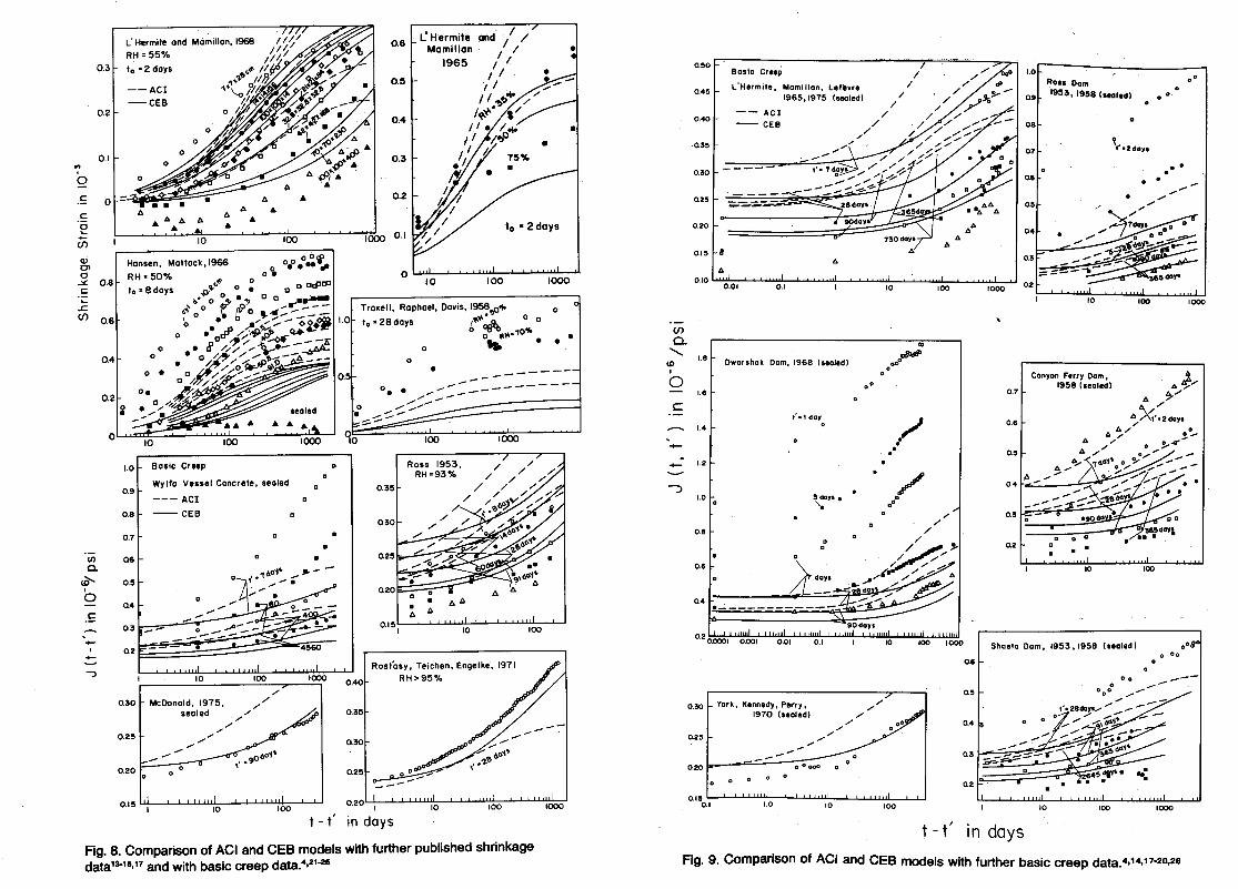
Fig. 8. Comparison of ACI and CEB models with further published shrinkage datal 3-15,17 and with basiC creep data.4

,21-2S

CIl Q.

.......... ID I

0

C

.....

..... J

o.~o Basic Creep

L'Hermite, Mamillan. Lef"vr. 0.4~

1965,1975 (sealed)

0.40

03~

030

02~

0.20

o.l~

0.10

1.8

1.6

1.4

1.2

1.0

0.8

0.6

0.4

0.30

02~

-- ACl -- CEB

--------------------

I>

I>

0.01 0.1

Dworshak Dam, 1968 (sealed)

,-, day o

York, Kennedy. Perry. 1970 (sealed)

............ .;­

..;-

.;-

..... -020~----~-~-~----~.~0~0$

,/

'"

10

co ~

otP o .

o·

./

,/ ,-

.. / . . / .. "

1>1> I>

100

0.6

.."

1000

0.7

0.6

O~

0.4

0.3

0.2

1.0 Ro •• Dam

0.9 19S3, 19S8 (_lid)

0 08

07 \'2dOYO

Q8

O~

04

02

Canyon. Ferry Dam I

1958 (.ealed)

I>

--" " •

10

• •

100

Shasta Dam, 1953, 1958 (sealed)

0.1 5 OL.I--.L-.L.J...u..wJI.-O-"-LJ..L.J.J..wIO-....I........I....L..WUJ.J,oo"-~-I..J 10 100

t - t' in days

00

.. .

o ••

1000

Fig. 9. Comparison of ACI and CEB models with further basic creep data.4,14,17-20,26

(/)

0.. '-..

ID

0 C

...--.

+-

+-

-----:>

1.0 L' Hermile, Mamillan, Lefevre, 1965,1971

RH: 50% 0.8

--Act -CEB

0.6

p.4

0.2

Tralell, Raphael, Davis, 1958 0 0

I.!:! 0

I' = 28 days 0.98

1.0 0

0

o.!:!

Hummel, el ai, 1962 ",,0

00

RH:65% --O.!:!

0.4 0

0.3

O.!:! Raslosy, 1975, RH :65%

0.4

0.3 o

0.2

1.0

0.8

0.6

0.4

0.2

•

L'Hermile, Mamillan, 1965

10

0.8

0.7

0.6

o.!:!

0.4

0.3

100 1000

Meyers and Maily, 1970 0 .,

D

I 0

RH =50% 0

D 0

D

10 100

Lamba"e, Mommens, 1976

0.6 Concrele P26, .P29 o

o

O.!:!

0.4 o

o 0

10 1<>0

o o

t - t I In days Fig. 10. Comparison of ACI and CEe models with published data on creep at drying.14,15,17,24,27-28

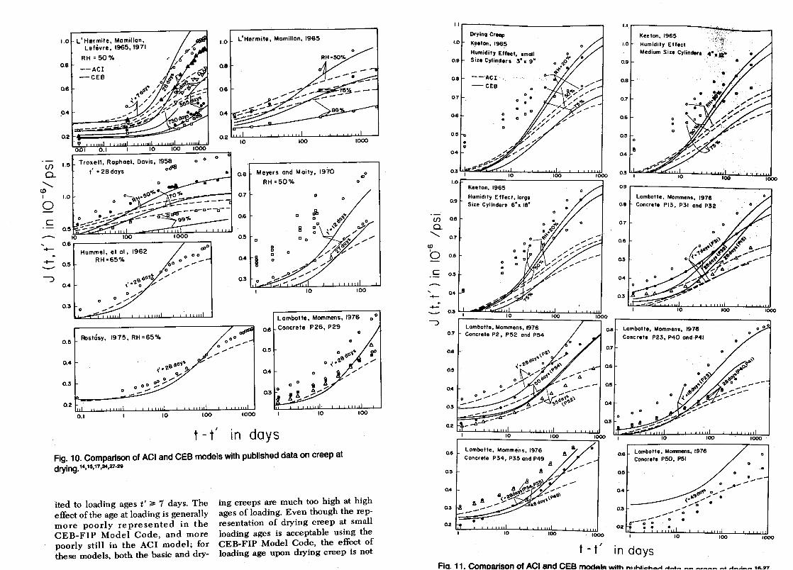
ited to loading ages t' ~ 7 days. The effect of the age at loading is generally more poorly represented in the CEB-FIP Model Code, and more poorly still in the ACI model; for these models, both the basic and dry-

ing creeps are much too high at high ages of loading. Even though the rep­resentation of drying creep at small loading ages is acceptable using the CEB-FIP Model Code, the effect of loading age upon drying creep is not

1.1 r---------------. 1.0

0.9

08

0.7

0.6

0.5

04

09

08

07

CD

'0 0.6

c 0.5

. o

Drying Creep

Keelon, 1965

Humidity Effect small Size Cylinder. '3" x 9"

--'ACI

-CEB

o

• o

Kee lon, 1965

• o

o

•

Humidily Effecl,large Size Cylinders S"X 18"

. o

•

~--------~~------~~-----r--~IOOO 08

07

06

__ - Of)

04

03

1000

t - t I

1.0

0.9

0.8

0.7

0.6

0

0.5

e 0.4

0.9,----------,-_----, Lambo"e, Mommens, 1976

08 Concrele PI3, P31 and P32

0.7

0.6

04

0.3

Lambo"e, Mommens, 1976

Concret. P23, P40 and P41

o 0 o

In days

o

1000

o

Fia. 11. ComDarison of ACI and CEe modelA with nllhli.,h ..... "'ft+ft ~~ ~.~~ _+ ... -.,~- 18_27

CIl > ;" 'r;; e I::..s .. CIl., ." a e .... Ilo

:oJ

~ .; .. ~ ~ fa • .!.

.. ~"; as ~ = .. ~.!

:1:1 ::s ~ -e <i' CIl

~l .s ~ f Ilo g U ~ 'tl .ti ...;:1:1 ., CiI

., or;; Q,)

>. = l~ ., ]~

~ i <i'

.9 i ~ ",i ~ ,91

~ CiI

~ = :e ., Ilo .~ ~ CIl 118. f = '" 0 Iloe .... ~ o~ .9 Ilo..c:

.. Ilo g 'tl'tl ~ CIl ., ..§ a

r:.1 ~ ~ CIl

" 01 CiI

.;

~

.; ... c 0 ,; ~ ~ 0 ~ >. § ..c: CIl - .... c ~ CIl 0

] -as"; :II 0 ft) e;o -;; or;;

'" ~ .::s >. .E .~ ~'tl"; E.i3 -;;; fa ., >. ... "; rIl - VJ (i ~ fa .9 11l !3 ..§ ~ ~ ~ ~ CIl r:.1::::.St; " ...;

~ ~ ~ ~ ~ ~ ao t-- t-- "" '" CiI

..

~ ~ ~ ~ ~ ~ ~ 12 <:> <:> t-- "" '" ...

~ ~ ~ ~ ~ ~ ~ 12 "" ...

., ., .,l:..c: ..c:l:..c: :§. CiI ... :§,CiI "':§.'" .. ..

0 0

= "; ~

&> ao 8l .~ = ~~ t-- t--

CiI < I:Q

~ 2! • ::s U r:.1 ll. ll."; u u I:Q I:Q I:Q >

3 e .3 :s ~ s

~ ~ ~ ~ ~ co "" CiI CiI ...

:5l ..s:: ..s:: ..s:: cS '" co <:> CiI co

Q,) = -= ~ .. 8. ~ ~. 0 CIl'~ ~ .s =rg!B;:e~ d ~o·~.5!-="!~O~" CIl =6 t;;CIlll·~=s.5!Qie~ • CIl .~ 2l Sol S ~ E ~"tl' -= . Ilo_ ~ 'Ot;;~S";;::CIl O.,..dCll Cll

- - 1lo .... 8...c:E .... ~CIl 1 i ~.~]!] ~ 1:a j ~ ~ ~ -< ~ U r::i rzl

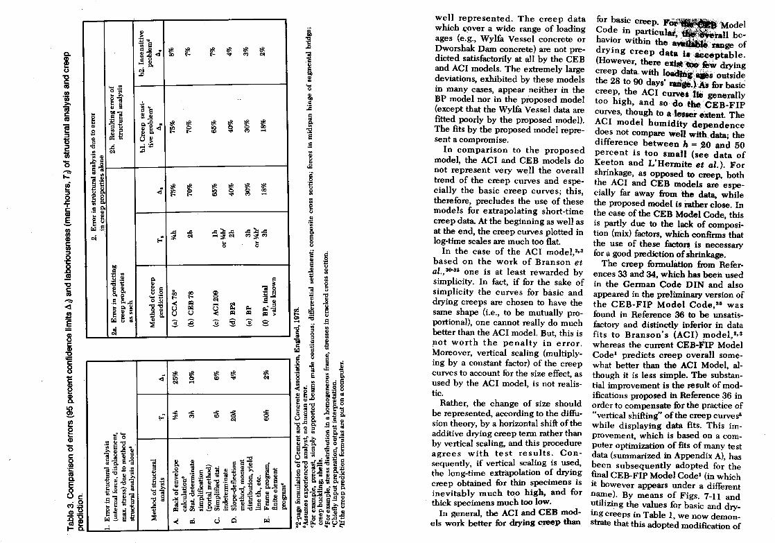
well represented. The creep data which c~ver a wide range of loading ages (e.g., Wylfa Vessel concrete or Dworshak Dam concrete) are not pre­dicted satisfactorily at all by the CEB and ACI models. The extremely large deviations, exhibited by these models in many cases, appear neither in the BP model nor in the proposed model (except that the Wylfa Vessel data are fitted poorly by the proposed model). The fits by the proposed model repre­sent a compromise.

for basic creep. Fci1'" -Model Code in particular; .. .rall .be­hav~or within the ~ range of drymg creep data iI~eeptable. (However, there e.i_·.~ .. "'drying creep data. with loadbl,.s outside the 28 to 90 days' ranaeJJ\s fOr basic creep, the ACI curveille generally too high, and so do the CEB-FIP curves, though to a lesser extent. The ACI model humidity dependence does not compare well With. data; the difference between h = 20 and 50 percent is too small (s~e data of Keeton and L'Hermite et ol.). For shrinkage, as opposed to creep, both the ACI and CEB models are espe­cially far away from the data, while the proposed model is rather close. In the case of the CEB Model Code, this is partly due to the lack of composi­tion (mix) factors, which confirms that the use of these factors is necessary for a good prediction of shrinkage.

In comparison to the proposed model, the ACI and CEB models do not represent very well the overall trend of the creep curves and espe­cially the basic creep curves; this, therefore, precludes the use of these models for extrapolating short-time creep data. At the beginning as well as at the end, the creep curves plotted in log-time scales are much too flat.

In the case of the ACI model,I,3 based on the work of Branson et al.,30032 one is at least rewarded by Simplicity. In fact, if for the sake of simplicity the curves for basic and drying creeps are chosen to have the same shape (Le., to be mutually pro­portional), one cannot really do much better than the ACI model. But, this is not worth the penalty in error. Moreover, vertical scaling (multiply­ing by a constant factor) of the creep curves to account for the size effect, as used by the ACI model, is not realis­tic.

Rather, the change of size should be represented, according to the diffu­sion theory, by a horizontal shift of the additive drying creep term rather than by vertical scaling, and this procedure agrees with test results. Con­sequently, if vertical scaling is used, the long-time extrapolation of drying creep obtained for thin specimens is inevitably much too high, and for thick specimens much too low.

In general, the ACI and CEB mod­els work better for drying creep than

The creep fOrmulation from Refer­ences 33 and 34, which has been used in the German Code DIN and also appeared in the preliminary version of the CEB-FIP Model Code,aII was found in Reference 36 to be unsatis­factory and distinctly inferior in data fits to Branson's (ACI) model,2,3 whereas the current CEB-FIP Model Code! predicts creep overall some­what better than the ACI Model, al­though it is less simple. The substan­tial improvement is the result of mod­ifications proposed in Reference 36 in order to compensate for the practice of "vertical shifting" of the creep curvesS

while displaying data fits. This im­provement, which is based on a com­puter optimization of fits of many test data (summarized in Appendix A), has been subsequently adopted for the fmal CEB-FIP Model Code! (in which it however appears under a different name). By means of Figs. 7-11 and utilizing the values for basic and dry­ing creeps in Table 1, we now demon­strate that this adopted modification of

References 33-35 does indeed bring

about a rather significant improve­

ment, mitigating part of the grevious criticism.

Nevertheless, as we see. from the

figures and Tables 1 and 2, the CEB­

FIP Model Code formulation1 is still

clearly inferior in data fits (confidence

limits). It is also much more limited in

scope than the BP model.4 The proce­

dure is not even simpler, although at

first it might appear so because fewer

formulas are used in the Model Code.

This is partly because many functions

are defined by graphs (16 curves). If

all the curves were defined by equa­

tions, as in other models, the Model

Code formulation would appear more

complicated than the BP model. For

computer programs, equations are of

course clearly preferable to graphs.

Formulas are also advantageous for

predictions especially when using

measured short-time values of creep.

In discussing the deviations from

the experimental data, we should ap­

preciate the importance of avoiding

the subjective element in selecting

the test data with which we compare

our model. When we make a totally

unbiased selection of test data (i.e.,

random, by casting a dice), the re­

sulting error of course should not sig­

nificantly depend on the number of

data sets used (unless this number is

too small, say six). However, any sub­

jective judgment in selecting the data

sets can be dangerously misleading.

This is illustrated in Table I(B). For

example (see Reference 4), if among

the 12 available shrinkage data sets4

one selects the 8 best fitted data sets

(which would certainly look to a

casual reader as sufficient experi­

mental verification), the confidence

limit obtained from comparing our

model to the test data drops from 52 to

21 percent and if one fits these 8 data

sets independently of those which

were left out, it drops to about 13 per­cent.4 (It was for this reason that prac-

tic ally all test data which could be

found in the literature were used in Reference 4.)

With regard to extensions beyond

the range of available test data

theoretical and conceptual aspect~ are, of course, very important too.

For their critical analysis, other works:'-7,\I,lo,41 are applicable.

Model Accuracy and Complexity

The fact that an increase in accuracy

of prediction is inevitably accom­

panied by an increase in complexity of

the model prompts us to ask: Is the

increase in complexity worthwhile?

The question must be viewed in con­

text of the entire structural analysis

process. The analysis of complex pre­

stressed concrete structures is fre­

quently performed by sophisticated

methods (e.g., computer frame

analysis, finite elements and elasto­

plastic methods), the error of which

might be less than 2 percent, whereas

the creep and shrinkage strains, which

are several times larger than the elas­

tic strains, are usually predicted by

models whose error exceeds 65 per­

cent with a 10 percent probability and

is much larger than the error in

strength. Such an approach makes lit­

tle sense. Optimally, the effort spent

on various tasks in the structural

analysi~ process should be commen­

surate with the expected accuracy

gain due to refinement of that task. A

rough illustrative comparison of this

type is attempted in Table 3. Although

the precise values in this table may be

disputed, they nevertheless give a

general idea of the problem. It is ap­

parent from this table that none of the

existing methods for creep prediction

is too complicated for all but creep-in­sensitive ~tructures.

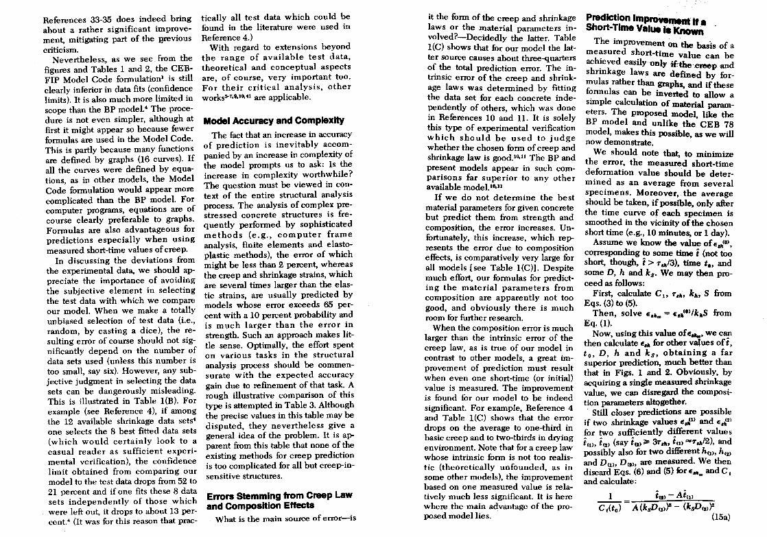
Errors Stemming from Creep Law and Composition Effects

What is the main source of error-is

it the form of th . e creep and shnnkage laws or the m t . I . Prediction Impro

Short-Time Value v::::... . a ena parameters In-

volved?-Decidedly the latter. Table

HC) shows that fur our model the lat­

ter Source causes about three-quarters

o~ ~e total prediction error. The in­tnnsiC error of the creep and shrink­

age laws was determined by fitting

the data set for each concrete inde­

~ndently of others, which was done

In References 10 and 11. It is solely

this type of experimental verification

which should be used to judge

wh~ther the chosen furm of creep and

shrinkage law is good,lo,l1 The BP and

pre~nt models appear in such com­par.Isons far superior to any other aVaIlable model.1o,u

If we do not determine the best

material parameters for given concrete but predict them from strength and

composition, the error increases. Un­

furtunately, this increase, which rep­

resents the error due to composition

effects, is comparatively very large fur

all models [see Table HC)]. Despite

~uch effort, our formulas for predict­Ing the material parameters from

composition are apparently not too

good, and obviously there is much room for further research.

When the composition error is much larger than the intrinsic error of the

creep law, as is true of our model in

contrast to other models, a great im­

provement of prediction must result

when ~ven one short-time (or initial)

value IS measured. The improvement

is found for Our model to be indeed

significant. For example, Reference 4

and Table I(C) shows that the error

drops on the average to one-third in

basi: creep and to two-thirds in drying

enVIronment. Note that for a creep law

whose intrinsic furm is not too realis­

tic (theoretically unfounded, as in

some other models), the improvement

based on one measured value is rela­tively much less significant. It is here

where the main advantage of the pro­posed model lies.

The improvement '._ measured short_tO on the basis of a

h' d Ime value can be ac ~eve easilyonlyif:th. shrInkage laws ar eereepand mulas rather than :ra d::;ned by for­formulas can b . p , and if these . I e Inverted to allow a

SImp e calculation of material

eters. The proposed model li~a.r:­BP model and unlike the' CE; 7: model, makes this possible. as we will now demonstrate.

We should note that, to m' . . the h mImlze

error, t e measured short-time

d~formation value should be deter­

mIn~d as an average from several

speCImens. Moreover,. the average

shou~d be taken, if possible. only after the tIme curve of each spe . . . clmen IS smoothed in the vicinity of the chosen

short time (e.g .• 10 minutes. or 1 day).

Assume we know the value of E (0)

corresponding to some time i (not ~~ short. though. i> T .. /3). time to, and

some D. h and ks . We may then pro­ceed as follows:

First, calculate C h T ,A. kA, S from Eqs. (3) to (5).

Then. solve E,A .. = E,.(O)/kAS from Eq. (1).

Now. using this value of E ..... we can then calculate E .. for other values of i to. D, hand ks, obtaining a fa; superior prediction, much better than

that in Figs. 1 and 2. Obviously, by

acquiring a single measured. shrinkage

value, we can disregard the composi­tion parameters altogether.

Still closer predictions are possible if two shrinkage values E_~t) and E (2)

... ,A

for!:Wo sU~ICiently d!fferent values t(U, t<J) (say t(2);;o 3r ... t(u .... T ".12), and

possibly also for two different h(U, h(2)

and DUh D(2h are measured We then discard Eqs. (6) and (5) for E", and C and calculate: .. 1

1 i(2) - Aim

C j(to) = A (ksDu»)Z - (ksD(2»)2 (l5a)

(I5b)

(I5c)

(I5d)

(15e)

(l5i)

E (2) E (1) - --./1- ___ ./1_ E.hoo - k (2)S - k (I)S /I (2) /I (1)

(l5g)

From the above equations we can predict E./I(t,to) for any other case.

Basic Creep If the elastic modulus or some

short-time strain value is known, the prediction accuracy approximately tri­ples.4 Assume we know the value of the conventional static modulus, which is here obtained as J at t - t' = ~t = 1 day, i.e.,

E(t') = lIJ(t' + M, t') The following procedure can then

be used: 1. Evaluate CP1' m, n and a from Eq.

(9). 2. Substitute these values along

withJ (t' + ~t, t') = liE (t'). and t - t' = ~t into Eq. (8) and solve for Eo:

Eo = E(f'}[l + CP1(t,-m + a)~tn] (16)

where~fn = 1" = 1.

3. Using this Eo value instead of that found from Eq. (9), substantially better predictions of J (t,t') at any t and t' can be obtained, much better than those in Figs. 3 and 4.

If we also measure one short-time creep valueJ1' e.g., for t -t' = t2 = 14 days, t' = 28 days, we further improve the prediction:

1. Calculate m, n and a from Eq. (9).

2. Write Eq. (8) twice, once for J at the aforementioned times, and once for liE as before; this yields a system of two linear equations for lIEo and cp1 /E o:

1.. + (t'-m + a) ~t CP1 = 1.. (I7a) Eo Eo E

3. Solving lIEo and CP1IEo, we can then predict J (t,t') for any t and t' from Eq. (8).

Other alternatives of course, are possible. For example:

1. Use Eq. (9) to get lIEo, m and a. 2. Noting that log Co = n log

(t -t') + log[(t,-m + a)cp1/Eo], write this relation for Co = (liE) - (lIEo) and for Co = J1 - lIEo (with t - t' = t2 = 14 days):

n log ~t + log .fJ = log (...!. - ...!. )-Eo E Eo

log(t,-m + a) (l8a)

n logt2 + log CP1= log(J1 -...!.)-Eo Eo

log(f'-m + a) (18b)

which is a system of two linear equa­ions for n and log (cp1IEo)' Solving them, we can obtain nand CP1IEo, upon which we can predict J (t,f') for any time f' and f from Eq. (8).

The latter prediction will normally differ somewhat from the previous one [Eq. (I7)]. It may, however, be advisable to carry out both predictions to get an idea of the range to expect. Various other alternative procedures are possible, too, but they require solving transcendental equations.

Drying Creep

If we can measure the value of J (t,t') for some relatively small t - t' value (perhaps t - t' ~ 7./1/10) and certain parameters t' , to, D, h, ks, we can again greatly improve the accu­racy:

1. Calculate Eo, CP1, m, n and a from Eq. (9) and also k;., Sa(t,t') from Eqs. (l2) and (13), and C o(t,t') from Eq. (8).

2. Then solve Ca(t,t' ,to) for these t t' and to ~alues from Eq. (l0), and als~ solve the CPa value from Eq. (11). _ 3. Now use this ~a value, instead of CPa from Eqs. (I2) and (14), to calculate J(t,t') for any other t, t' , to, D, h and ks, greatly improving the accuracy and at the same time eliminating the need for composition parameters.

Further accuracy is possible if we, in addition, have the experimental elastic modulus E (e.g., for t - t' = 1 day). Then we do not need to estimate Eo from Eq. (9), as above, but instead we can calculate it from Eq. (8), as in case of basic creep. We then proceed using Steps 1, 2, 3 as described above.

It is interesting to note that by hav­ing some measurements we can disre­gard the composition parameters in the BP model.4 For this, we need to know the measured values of: (1) shrinkage at two different times or thicknesses, (2) elastic modulus and one short-time basic creep value (for, say, t -t' = 7 days) to predict basic creep, and (3) elastic modulus and two creep values to predict drying creep.

It is also worth mentioning that, be­cause graphs are employed rather than formulas, the CEB-FIP model be-

comes too cumbersome to use effec­tively when a measured short-time creep value or two shrinkage values are given.

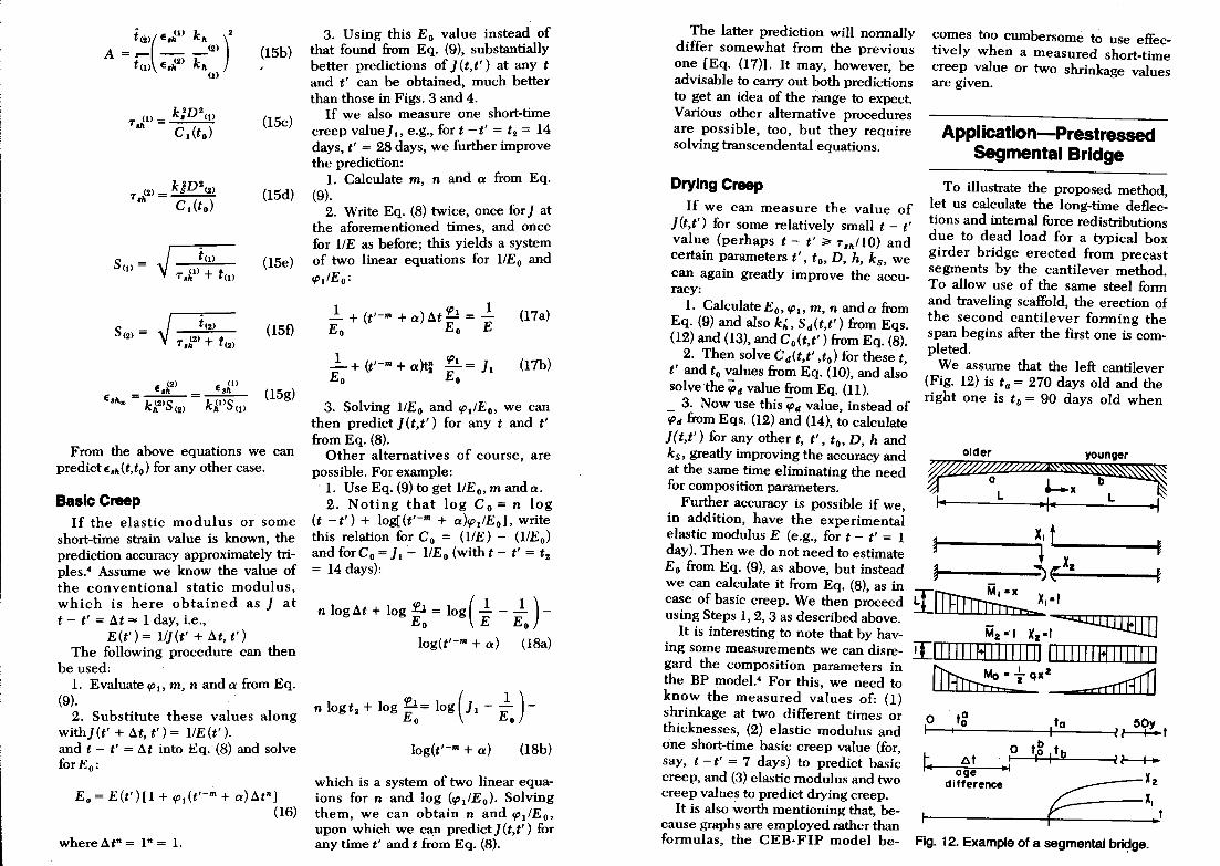
Application-Prestressed Segmental Bridge

To illustrate the proposed method, let us calculate the long-time deflec­tions and internal force redistributions due to dead load for a typical box girder bridge erected from precast segments by the cantilever method. To allow use of the same steel form and traveling scaffold, the erection of the second cantilever forming the span begins after the first one is com­pleted.

We assume that the left cantilever (Fig. 12) is ta = 270 days old and the right one is tb = 90 days old when

older younger

o ~t I

age -I difference

Fig. 12. Example of a segmental bridge.

they are joined at midspan. The join­ing is continuous or by a hinge. The cantilevers are connected without any jacking, and so the force in the joint is zero at the beginning. For simplicity we assume that both cantilevers are fixed at their ends.

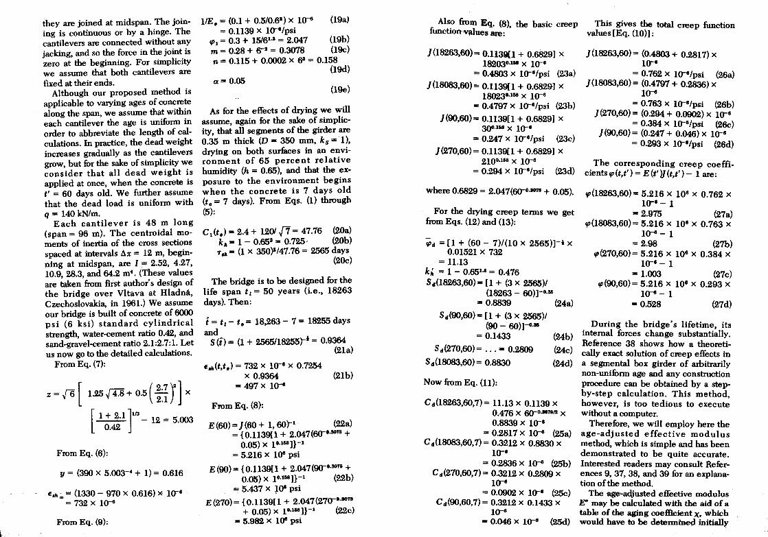
Although our proposed method is applicable to varying ages of concrete along the span, we assume that within each cantilever the age is uniform in order to abbreviate the length of cal­culations. In practice, the dead weight increases gradually as the cantilevers grow, but for the sake of simplicity we consider that all dead weight is applied at once, when the concrete is t' = 60 days old. We further assume that the dead load is uniform with q = 140kN/m.

Each cantilever is 48 m long (span = 96 m). The centroidal mo­ments of inertia of the cross sections spaced at intervals .1x = 12 m, begin­ning at midspan, are 1= 2.52, 4.27, 10.9,28.3, and 64.2 m4. (These values are taken from first author's design of the bridge over Vltava at Hladnl'l, Czechoslovakia, in 1961.) We assume our bridge is built of concrete of 6000 psi (6 ksi) standard cylindrical strength, water-cement ratio 0.42, and sand-gravel-cement ratio 2.1:2.7:1. Let us now go to the detailed calculations.

From Eq. (7):

z = .[6 [ 1.25 ~ 4.8 + 0.5 ( ::~ r] x

[ 1 + 2.1 ]1/3 _ 12 = 5.003

0.42

From Eq. (6):

y = (390 X 5.003-4 + 1) = 0.616

Ella';' = (1330 - 910 x (}.616) x 1(18 = 732 X 1(18

From Eq; (9):

I/E. = (0.1 + 0.5/0.61 ) x 1(18 (19a) = 0.1139 x 1(18/psi

1P1 = 0.3 + 15161.1 = 2.047 (19b) m = 0.28 + ()I = 0.3078 (19c) n = 0.115 + 0.0002 x 63 = 0.158

(19d) a= 0.05

(1ge)

As for the effects of drying we will assume, again for the sake of simplic­ity, that all segments of the girder are 0.35 m thick (D = 350 mm, ks = 1), drying on both surfaces in an envi­ronment of 65 percent relative humidity (h = 0.65), and that the ex­posure to the environment begins when the concrete is 7 days old (t. = 7 days). From Eqs. (1) through (5):

C 1(t.) = 2.4 + 1201.[7 = 47.76 (20a) k" = 1 - 0.653 = 0.725- (20b) T IIa = (1 x 35O}I/47.76 = 2565 days

(2Oc)

The bridge is to be designed for the life span t, = 50 years (i.e., 18263 days). Then:

i = t , - t. = 18,263 - 7 = 18255 days and

8 (i) = (1 + 2565/18255)""1 = 0.9364 (21 a)

EIIa(t,t.) = 732 x 1(18 x 0.7254 x 0.9364 (21b)

= 497 x 1(18

From Eq. (8):

E(60) = J(60 + 1,60)""1 (22a) = {0.1139[1 + 2.047(60-°·3078 +

0.05) X l o.158 ]}-1 = 5.216 x lOS psi

E (90) = {0.1139[1 + 2.047(90-°·3078 + 0.05) x lo.158]}-1 (22b)

= 5.437 x ~OS psi

E(270)= {0.1l39[1 + 2.047{27(1o.3878 + 0.05) X l o.1118 ]}-1 (22c)

= 5.982 x lOS psi

Also from Eq. (8) the basic creep function values are: ' This gives the total creep function

values [Eq. (10)]:

J (18263,60) = 0.1139(1 + 0.6829] x 182038.l118 x 1(18

J(l8263,60)= (0.4803 + 0.2817) x 1(1'

= 0.4803 x l(1s/psi (23a) = 0.762 x 1(1'/psi (26a) J(18083,60) = (0.4797 + 0.2836) x J(18083,60) = 0.1139[1 + 0.6829] x

180238.l118 X 1(18 1(1' = 0.4797 x 1(18/psi (23b) = 0.763 x 1(1'/psi (26b)

J{270,60) = (0.294 + 0.09(2) x 1(18 = 0.384 x 1(1'/psi (26c)

J(90,60) = (0.247 + 0.046) x 1(1'

J(90,60) = 0.1139[1 + 0.6829] x 3()O.1118 x 1(18

= 0.247 x 1(18/psi (23c)

J{270,60) = 0.1139[1 + 0.6829] x = 0.293 x l(18/psi (26d)

210°·1118 x 1(18 = 0.294 x 1(18/psi The corresponding creep coeffi­

(23d) cients IP (t,t') = E (t'}J (t,t') - 1 are:

where 0.6829 = 2.047(60-0•3078 + 0.05).

For the drying creep terms we get from Eqs. (12) and (13):

~" = [1 + (60 - 7)/(10 x 2565)]-1 x 0.01521 x 732

= 11.13 kit = 1 - 0.65l.li = 0.476 8,,(18263,60)= [1 + (3 x 2565)/

(18263 - 60)]-0.311 = 0.8839 (24a)

8,,(90,60)= [1 + (3 x 2565)/ (90 - 6O)]-o.as

= 0.1433 (24b)

8 ,,(270,60)= ... = 0.2809 (24c)

8,,(18083,60)= 0.8830 (24d)

Now from Eq. (11):

C,,(I8263,60,7)= 11.13 x 0.1139 x 0.476 x 60-°.307811 x 0.8839 X 1(1'

= 0.2817 x 1(18 (25a) C,,(18083,60,7) = 0.3212 x 0.8830 x

1(1-= 0.2836 x 1(1' (25b)

C,,{270,60,7)= 0.3212 x 0.2809 x 1(18

= 0.0902 X 1(18 (25c) C,,(90,60,7) = 0.3212 x 0.1433 x

1(1' = 0.046 x 1(18 (25d)

1P(18263,60) = 5.216 x 10' x 0.762 X

1(1' - 1 = 2.975 (27a)

1P(18083,60) = 5.216 x 108 x 0.763 X

1(18 - 1 = 2.98 (27b)

1P(270,60) = 5.216 x 108 x 0.384 X 1(18 - 1

= 1.003 (27c) 1P(90,60) = 5.216 x 108 x 0.293 X

1(18 - 1 = 0.528 (27d)

During the bridge's lifetime, its internal forces change substantially. Reference 38 shows how a theoreti­cally exact solution of creep effects in a segmental box girder of arbitrarily non-uniform age and any construction procedure can be obtained by a step­by-step calculation. This method, however, is too tedious to execute without a computer.

Therefore, we will employ here the age-adjusted effective modulus method, which is simple and has been demonstrated to be quite accurate. Interested readers may consult Refer­ences 9, 37, 38, and 39 for an explana­tion of the method.

The age'-adjusted effective modulus E" may be calculated with the aid of a table of the aging coefficient X, which would have to be determined initially

for our creep function. W~ may, how­ever, dispense with a table of X and calculate E" as:

E"(t t') = E (t') - R (t,t') (28) , tp(t,t')

where R (t,t') is the relaxation func­tion, for which recently a general and fairly accurate approximate formula has been established:40

R (t,t') = ;(:.~ - ) (~:~51) X

( }(t' +€,t') _ 1) (29a) }(t,t - €)

where € = (t-t' )/2 (29b)

To use Eq. (29) we need to know the following additional values, cal­culated similarly as before: For t = 18083, t' = 90:

}b(t' + €,t') = 0.409 x 100a/psi (30a)

where € = 8996 days,}b = Eo-t + Co = part of] due to basic creep [Eq. (10)];

~ = 11.12, Sd = 0.8055, Cd = 0.243 x 100a/psi (30b)

}(t' + €,t') = (0.409 + 0.243) x 100a

= 0.652 x 100a/psi (30e) }b(t,t - €)= 0.2225 x 100a/psi (31a)

~d = 9.5709, Sd = 0.80548, Cd = 0.1028 x 100a/psi (31b)

}(t,t - €) = (0.2225 + 0.1028) x 100a

= 0.3253 x 10-8/psi (31c)

For t = 18263, t' = 270:

}b(t' + €,t') = 0.3395 x 100a/psi (32a) ~d = 11.08, Sd = 0.8093, Cd = 0.2054 x 100a/psi (32b)

} (t' + € ,t' ) = (0.3395 + 0.2054) x 100a

= 0.5449 x 100a/psi (32c) } b(t,t - €) = 0.2221 x 100a/psi (33a)

~d = 9.546, Sd = 0.8055, Cd = 0.1022 x 10-8/psi (33b)

} (t,t - ~) = (0.2221 + 0.1022) x 10-& = 0.3243 x lo-a/psi (33c)

Fort = 18,063, t' = 90:

}b(t,t') = 0.4432 x 10-8 /psi (34a) ~d = 11.188, S d = 0.8828,

Cd = 0.2662 x 100a/psi (34b) } (t,t') = (0.3243 + 0.2662) x 100a

= 0.5905 x 100a/psi (34c)

Fort = 18263; t' = 270:

} b(t,t') = 0.3644 x 10-8/psi (35a) ~d = 11.08, Sd = 0.8828, Cd = 0.2240 x 10-8 /psi (35b)

}(t,t') = (0.3644 + 0.2240) x 10-8

= 0.5884 x 10-8 /psi (35c)

Fort = 18263, t' = t- 1:

}b(t,t') = 0.1369 x 10-8 /psi (36a) ~d = 8.512, S d = 0.04363, Cd = 0.00445 x 100a/psi (36b)

} (t,t') = (0.1369 + 0.00445) x 10-8

= 0.1414 x 100a/psi (36c)

For t = 90, t' = t - 1:

} b(t,t') = 0.1841 x 100a/psi (37a) ~d = 11.12, Sd = 0.04363, Cd = 0.01318 x 10-8/psi (37b)

} (t,t') = (0.1841 + 0.01318) x 100a

= 0.1973 x 100a/psi (37c)

For t = 270, t' = t - 1:

}b(t,t') = 0.1672 x 100a/psi (38a) ~d = 11.08; Sd = 0.04363,

Cd = 0.0111 x 10-8/psi (38b) }(t,t') = (0.1672 + 0.0111) x 100a

= 0.1783 x 100a/psi (3Bc)

Now, from Eq. (29):

R (18263,270) = (0.99210.5884) -(0.11510.1414) x [(0.5449/0.3243) - 1]

= 1.133 x 100/psi (39a) R(18083,90) = ... = 0.5813 x 10'/

psi (39b) E/J" = E"(18263,270)

= (5.982 - 1.133) x 10'/2.52 = 1.924 x 10'/psi (39c)

E;' = E"(l8083,90) = 1.704 x lOS/psi (39d)

Note that the corresponding aging piloeftlcients, which are used in Refer­·~s 9, 38, and 39 but are not needed here, are (E - E")/E" f/J or 0.849 and 0.770.

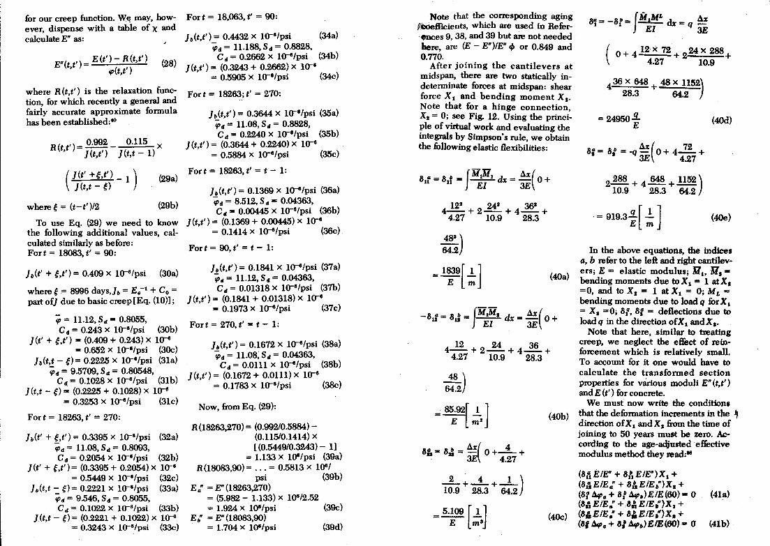
After joining the cantilevers at midspan, there are two statically in­determinate forces at midspan: shear force X t and bending moment X •. Note that for a hinge connection, XI = 0; see Fig. 12. Using the princi­!Jle of virtual work and evaluating the mtegrals by Simpson's rule, we obtain the fOllowing elastic flexibilities:

.. /J .. b JMtMt d .:1x( 011 = 011 = -- X = - 0 + EI 3E

122 24' 36' 4-=-- + 2-- + 4-- +

4.27 10.9 28.3

~) 64.2

= 1~9[ !] (40a)

-3tf = 3J = fMtM• dx = .:1x( 0 + EI 3E

~+2 24 +4~+ 4.27 10.9 28.3

48 ) 64.2

= SS.92[ 1. ] E ma

8 /J 8 b .:1x( 4 .- 21 = - 0+-+ . 3E 4.27

....L+-i....+-.L) 10.9 28.3 64.2

(40b)

=~ [1.J (4Oc) E ma

8/J - -8/> - JM,ML dx .:1x t- t - EI = q 3E

( 0 + 4 12· x 72 + 224 x 288 +

4.27 10.9

4 36 x 648 + 48 x 115~\ 28.3 64.2 J

= 24950.9... E

(40d)

8: = 8/ = -q .:1x (0 + 4...!!. + 3E 4.27

2288 + 4 648 +~) 10.9 28.3 64.2

,= 919.3 ~ [ ! ] (4Oe)

In the above equations, the indices a, b refer to the left and right cantilev­ers; E = elastic modulus; M., M,. bending moments due to X I = 1 at X. =0, and to X. = 1 at Xt = 0; ML -bending moments due to load q fOr X 1

= XI =0; 8[, 8: = deflections due to loadq in the direction of Xl andX •.

Note that here, .similar to treating creep, we neglect the effect of rein­forcement which is relatively small. To account for it one would have to calculate the transformed section properties for vanous moduli E" (t,t') and E (t') for concrete.

We must now write the conditions that the deformation increments in the ~ direction of X 1 andX. from the time of joining to 50 years must be zero. Ac­cording to the age-adjusted effective modulus method they read:·

(3t'1E/E" + 8/1 E/E")X1 + (8AEIE/J" + 8&EIE/>")X. + (8t.:1f{J/J + 8/ .:1f{J,,)EIE(60) == 0 (41 a) (8/tEIE: + a/tEIE,,")X, + (BjEIE." + al,EIE{)X. + (al.:1f{J/J + 8/.:1f{J.)EIE(60) - 0 (41b)

Since ~'Pa = 'P(l8263,60) 'P(270,60)

= 2.975 - 1.003 = 1.972 (42 a)

~'Pb = 'P(18083,60) - 'P(90,60) = 2.98 - 0.528 = 2.452

(42b)

We now have:

1O-6[ (1.924-1 + 1.704-1 )1839 X 11m + (-1.924-1 + 1.704-1 )85.92 X z/m 2 + (l.972 - 2.452)24950 q/5.216] = 0

(43a) 1O-6[ (-1.924-1 + 1.704-1 )85.92 X jIm + (1.924-1 + 1.704-1 )5.109Xz/m 2 -(l.972 + 2.452)919.3 q/5.216] = 0

(43b) or 2035 Xl + 5.766Xs = 2296[m2]q (44a) 5.766X 1 + 5.654X J = 780.0[m2]q

(44b)

From the above, we can solve for the desired force and moment:

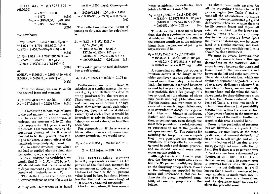
Xl = 0.740q[m] = 103.6 kN (45a) XI = 137.2q[m] = 19208 kNm (45b)

It is interesting to note that, relative to the end moment due to self weight for the case of no connection at midspan, the moment ± (48m )X I due to Xl represents ±3.1 percent and Xz represents 11.9 percent, causing the maximum change of the fixed-end moment to be 15.0 percent from join­ing to 50 years. A creep effect of this magnitude is certainly significant.

For an elastic structure upon which the load is applied after the fmal stat­ical system (Le., a system with a con­nection at midspan) is established, we would find Xl = 0, X2 = 179.9q[m2]. We should note that the value of the ~idspan momentXs due to creep is 76 percent of this elastic value of X •.

The deflection of the older can­tilever at midspan at time of joining is:

~l = 8f 'P(270,60) where 8f is based

on E = E (60 days). Consequent­ly:

~l = (24950/5.216 X 106 psi) x 1.003 = 0.OOO6957q[m2IkN] = 0.0974 m

(46)

The deflection from the instant of joining to 50 years may be calculated as:

~z = (8 11X I + 8I fXz)EIEd' + 8f ~'P(JEIE(60)

= (1839 X 0.740 - 85.92 x 137.2q )/(1.924 x 106 ) psi + 24945q x 1.972/(5.216 x 106 )

= 0.OOO582q1kN = 0.0814 m (47)

This value gives the total deflection due to self weight:

~l + ~2 = 0.0974 + 0.081 = 0.178 m

Furthermore, one would have to calculate in a similar manner the val­ues Xl' X z and deflections due to creep produced by the prestress. These tend to offset the above values and one may even obtain a design where they almost cancel each other. However, because of the statistical variability of each effect, it would be imprudent to rely in design on such "almost canceled values," as has often been done.

For comparison, if there were a hinge rather than a continuous con­nection at midspan, we would have:

Xz = 0 and 2035X I - 2296q[m 2] = 0

or Xl = 1.128q[m] = 158.0 kN

The corresponding moment (48m )X I repre sents as much as 4.7 percent of the fixed-end moment for no connection at midspan, Le., almost 11f2-times as much as the 3.1 percent value found before, but about 3-times less than the total maximum change of 15.0 percent computed previously.

Also for comparison, if there were a

hinge at midspan the deflection from joining to 50 years would be

~I = 811X I EIEaw + ~'Pa8f EIE (60) = (1839 x 1.128)/1.924 x 106 psi +

(24945 x 1.972)/5.216 x 106 psi = 0.00152q1kN = 0.21 m (48)

This deflection is 2.58-times larger than that for a continuous connection at midspan. The change of slope in the younger cantilever at the midspan hinge from the moment of joining to 50 years would be:

(JI = 81\XI EIE';' + ~'Pb8t EIE (60) = (85.92 x 1.128q)/l.704 x 106 psi

+ (919.3 x 2.452)/5.216 x 106 psi = 0.0099 radians = 0.57 deg (49)

A somewhat smaller but opposite rotation occurs at the hinge in the older cantilever, causing relative rota­tion of more than 1 deg due to dead load. This rotation is reduced by creep caused by the prestress. Nevertheless, it is probable that a fast passage of a heavy truck at this change of slope may cause non-negligible vibrations. For this reason, and even more so be­cause of the much larger deflections, it is imprudent to design the segmen­tal bridge with hinges at midspan. Rather, one should always use con­tinuous connections, even though one must then provide extra reinforcement or prestress to resist the positive midspan moment XI. The reasons for avoiding the hinge become compel­ling if one considers the statistical variability of creep effects, currently ignored in codes and design practice; and we should now add some com­ments on this problem.

Although this is not done in prac­tice, the designer should also calcu­late the 95 percent confidence limits on the foregoing creep effects. Based on the information supplied in this paper and Reference 4, this can be done for the overall statistical varia­bility of concrete properties in the bridge.

To obtain these limits we consider all the preceding I-values to be 29 percent higher (see Table 1) and re­peat all the calculations obtaining upper confidence limits on X X and 1, 2, deflections. Then we aSSume them to be 29 percent lower and repeat all calculations, obtaining the lower con­fidence limits. The effects of creep due to the prestressing forces (plus the effects of shrinkage) can be calcu­lated in a similar manner, and their upper and lower confidence limits should be also established.

We must be aware, however, that we do not currently have a firm un­derstanding on the statistical differ­ences in creep between the upper and lower fibers of the cross section and between the left and right cantilevers. These statistical variations, which un­doubtedly represent important causes of excessive deflections observed in concrete structures, are not mutually independent, and therefore the confi­dence limits for their differences must be less than those deduced on the basis of Table 1. Thus, one needs to obtain information on joint probability distributions within the cross section of the errors of creep in the upper and lower fibers of the section. Further re­search in this area is needed here.

Errors in the prediction of prestress loss are likewise very important. For example, we may have, as the mean prediction, a downward deflection of 20 cm due to self weight, and an up­ward deflection of 18 cm due to pre­stress, giving a net mean deflection of 2 cm. But if there is a 10 percent error in prestress, we have a downward de­flection of 20 - 18(1 - 0.1) = 4 cm. Hence, we see that a 10 percent error in prestress loss causes a 100 percent error in the net deflection. It is well known that a small difference of two large numbers is much more inaccu­rate than the numbers themselves and the designer must be carefui about this potential error.

iiI;;

Conclusions

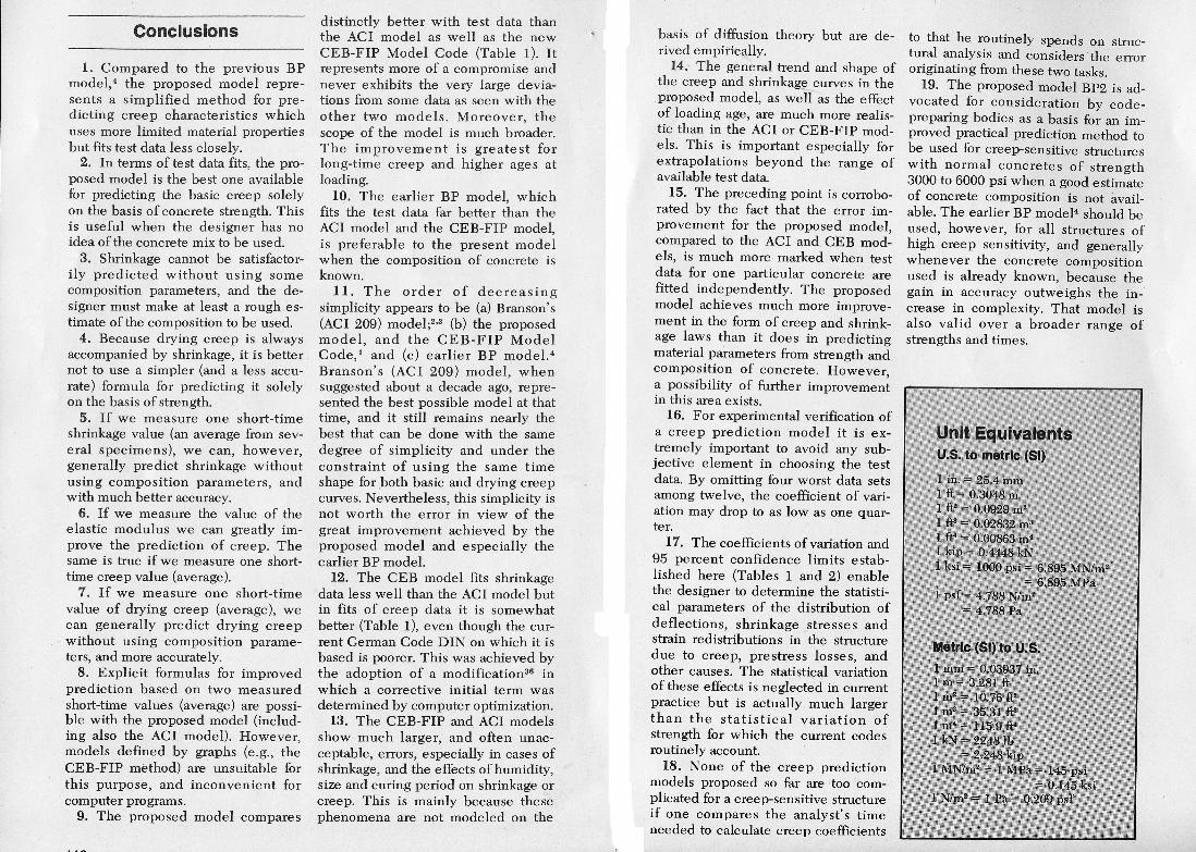
1. Compared to the previDus BP model,4 the proposed model repre­sents a simplified method for pre­dicting creep characteristics which uses more limited material properties but fits test data less closely.

2. In terms of test data fits, the pro­posed model is the best one available for predicting the basic creep solely on the basis of concrete strength. This is useful when the designer has no idea of the concrete mix to be used.

3. Shrinkage cannot be satisfactor­ily predicted without using some composition parameters, and the de­signer must make at least a rough es­timate of the composition to be used.

4. Because drying creep is always accompanied by shrinkage, it is better not to use a simpler (and a less accu­rate) formula for predicting it solely on the basis of strength.

5. If we measure one short-time shrinkage value (an average from sev­eral specimens), we can, however, generally predict shrinkage without using composition parameters, and with much better accuracy.

6. If we measure the value of the elastic modulus we can greatly im­prove the prediction of creep. The same is true if we measure one short­time creep value (average).

7. If we measure one short-time value of drying creep (average), we can generally predict drying creep without using composition parame­ters, and more accurately.

8. Explicit formulas for improved prediction based on two measured short-time values (average) are possi­ble with the proposed model (includ­ing also the ACI model). However, models defined by graphs (e .g., the CEB-FIP method) are unsuitable for this purpose, and inconvenient for computer programs.

9. The proposed model compares

distinctly better with test data than the ACI model as well as the new CEB-FIP Model Code (Table 1). It represents more of a compromise and never exhibits the very large devia­tions from some data as seen with the other two models. Moreover, the scope of the model is much broader. The improvement is greatest for long-time creep and higher ages at loading.

10. The earlier BP model, which fits the test data far better than the ACI model and the CEB-FIP model, is preferable to the present model when the composition of concrete is known.

11. The order of decreasing simplicity appears to be (a) Branson's (ACI 209) model;2.3 (b) the proposed model; and the CEB-FIP Model Code,! and (c) earlier BP model.' Branson's (ACI 209) model, when suggested about a decade ago, repre­sented the best possible model at that time, and it still remains nearly the best that can be done with the same degree of simplicity and under the constraint of using the same time shape for .both basic and drying creep curves. Nevertheless, this simplicity is not worth the error in view of the great improvement achieved by the proposed model and especially the earlier BP model.

12. The CEB model fits shrinkage data less well than the ACI model but in fits of creep data it is somewhat better (Table 1), even though the cur­rent German Code DIN on which it is based is poorer. This was achieved by the adoption of a modification36 in which a corrective initial term was determined by computer optimization.

13. The CEB-FIP and ACI models show much larger, and often unac­ceptable, errors, especially in cases of shrinkage, and the effects of humidity, size and curing period on shrinkage or creep. This is mainly because these phenomena are not modeled on the

basis of diffusion theory but are de­rived empirically.

14. The general trend and shape of the creep and shrinkage curves in the proposed model, as well as the effect of loading age, are much more realis­tic than in the ACI or CEB-FIP mod­els. This is important especially for extrapolations beyond the range of available test data.

15. The preceding point is corrobo­rated by the fact that the error im­provement for the proposed model, compared to the ACI and CEB mod­els, is much more marked when test data for one particular concrete are fitted independently. The proposed model achieves much more improve­ment in the form of creep and shrink­age laws than it does in predicting material parameters from strength and composition of concrete. However, a possibility of further improvement in this area exists.

16. For experimental verification of a creep prediction model it is ex­tremely important to avoid any sub­jective element in choosing the test data. By omitting four worst data sets among twelve, the coefficient of vari­ation may drop to as low as one quar­ter.

17. The coefficients of variation and 95 percent confidence limits estab­lished here (Tables 1 and 2) enable the designer to determine the statisti­cal parameters of the distribution of deflections, shrinkage stresses and strain redistributions in the structure due to creep, prestress losses, and other causes. The statistical variation of these effects is neglected in current practice but is actually much larger than the statistical variation of strength for which the current codes routinely account.

18. None of the creep prediction models proposed so far are too com­plicated for a creep-sensitive structure if one compares the analyst's time needed to calculate creep coefficients

to that he routinely spends on struc­tural analysis and considers ' the error originating from these two tasks.

19. The proposed model BP2 is ad­vocated for consideration by code­preparing bodies as a basis for an im­proved practical prediction method to be used for creep-sensitive structures with normal concretes of strength 3000 to 6000 psi when a good estimate of concrete composition is not avail­able. The earlier BP model' should be used, however, for all structures of high creep sensitivity, and generally whenever the concrete composition used is already known, because the gain in accuracy outweighs the in­crease in complexity. That model is also valid over a broader range of strengths and times.

Unit Equivalents u.s. to metric (SI)

1 in. = 25.4 rnrn 1 ft = 0.3048 rn 1 ft2 = 0.0929 rn2

1 ft3 = 0.02832 rna 1 ft4 = 0.00863 rn4

1 kip = 0.4448 kN 1 ksi = 1000 psi = 6.895 MN/rn2

= 6.895 MPa 1 psf= 4.788 N/rn2

= 4.788 Pa

Metric (SI) to U.S.

1 rnrn = 0.03937 in. 1 rn = 3.281 ft 1 rn2 = 10.76 ft2

rna = 35.31 ft3 1 rn4 = 115.9 ft4 ' 1 kN = 2248lb

= 2.248 kip 1 MN/rn2 = 1 MPa = 145 psi

= 0.145 ksi 1 N/rn' = 1 Pa = 0.209 ps~

REFERENCES 1. CEB-FIP Model Code for Cencrete

Structures, Commite Eurointerna­tional du Beton'-Federation Inter­nation ale de la Precontrainte, CEB Bulletin No. 1241125-E, Paris 1978.

2. ACI Committee 209/11 (chaired by D. E. Branson, "Prediction of Creep, Shrinkage and Temperature Effects in Concrete structures," ACI-SP27, De­signing for Effects of Creep, Shrink­age and Temperature, American Con­crete Institute, Detroit, 1971, pp. 51-93.

3. ACI Committee 209/11 (chaired by D. Carreira), Revised Edition of Refer­ence 2, 1978 (to be published).

4. Bafant, Z. P., and Panula, L., "Practi­cal Prediction of Time-Dependent Deformations of Concrete," Materials and Structures, Parts I and II: V. ll, No. 65, 1978, pp. 307-328, Parts III and IV: V. ll, No. 66, 1978, pp. 415-434, Parts V and VI: V. 12, No. 69, 1979, pp. 169-183.

5. Baiant, Z. P., and Osman, E., "On the Choice of Creep Function for Standard Recommendations on Practical Analysis of Structures," Cement and Concrete Research, V. 5, 1975, pp. 129-138, 631~1; V. 6, pp. 149-153; V. 7, pp. ll9-130; V. 8, pp. 129-130.

6. Baiant, Z. P., and Thonguthai, W., "Optimization Check of Certain Re­cent Practical Formulations for Con­crete Creep," Materials and Struc­tures (RlLEM, Paris), V. 9, 1976, pp. 91-96.

7. Baiant, Z. P., and Kim, S. S., "C1lIl the Creep Curves for Different Loading Ages Diverge?" Cement and Concrete Research, V. 8, September 1978, pp. 60l~11. '

8. Baiant, Z. P., and Panula, L., "A Note on Limitations of a Certain Creep Function Used in Practice," Materials and Structures, V. 12, No. 67, 1979, pp.29-31.

9. Baiant, Z. P., "Theory of Creep and Shrinkage in Concrete Structures: A Precis of Recent Developments," Me­chanics Today, Pergamon Press, V. 2, 1975, pp. 1-93.

10. Baiant, Z. P., and Osman, E., "Double Power Law for Basic Creep of Con­crete," Materials and Structures (RILEM, Paris), V. 9, No. 49, 1976, pp. 3-11.

ll. Baiant, Z. P., Osman, E., an~ Thon-

guthai, W., "Practical Fonnulation of Shrinkage and Creep of Concrete," Materials and Structures (RILEM, Paris), V. 9, No. 54, 1976, pp. 395-406.

12. Baiant, Z. P., and Najjar, L. J., "Non­Linear Water Diffusion in Non-satu­rated Concrete," Materials and Structures (RILEM, Paris), V. 5, 1972, pp.3-20.

13. Hansen, T. C., and Mattock, A. H., "Influence of Size and Shape of Member on the Shrinkage and Creep of Concrete," ACI Journal, Proceed­ings V. 63,1966, pp. 267-290.

14. L'Hermite, R., and Mamillan, M., "Retrait et fluages des betons," Annales de l'Institut Technique du Batiment et des Travaux Publics (Supplement), V. 21, No. 249, 1968, p. 1334; "Nouveaux resultats et recentes etudes sur Ie fluage du beton," Materials and Structures, V. 2, 1969, pp. 35-41; Mamillan, M., Bouineau, A., "Influ­ence de la dimension des eprouvettes sur Ie retrait," Annales Institut Technique du Batiment et des Travaux Publics (Supplement), V. 23, No. 270, 1970, pp. 5~.

15. Troxell, G. E., Raphael, J. M., and Davis, R. W., "Long-Time Creep and Shrinkage Tests of Plain and Rein­forced Concrete," Proceedings, ASTM V. 58,1958, pp. llOI-ll20.

16. Keeton, J. R., "Study of Creep in Con­crete," Technical Reports R333-1, R333-1I, R333-III, 1965, U.S. Naval Civil Engineering Laboratory, Port Hueneme, California.

17. L'Hennite, R. G., Mamillan, M., and Lefevre, C., "Nouveaux resultats de recherches sur la deformation et la rupture du beton," Annales de l'In­stitut Technique du Batiment et des Travaux Publics, V. 18, No. 207-208, 1965, pp. 323-360. See also Interna­tional Conference on the Structure of Concrete, Cement and Concrete As­sociation, London, 1968, pp. 423-433.

18. Hanson J. A., "A Ten-Year Study of Creep Properties of Concrete," Con­crete Laboratory Report No. SP-38, U.S. Department of the Interior, Bureau of Reclamation, Denver, Col­orado, July 1953.

19. Harboe, E. M., et al., "A Comparison of the Instantaneous and the Sustained Modulus of Elasticity of Concrete," Concrete Laboratory Report No.

C-854, Division of Engineering LaboratOries, U.S. Department of the Interior, Bureau of Reclamation, Den­ver, Colorado, March 1958.

20. Pirtz, D., "Creep Characteristics of Mass Concrete for Dworshak Dam," Report No. 65-2, Structural Engineer­ing Laboratory, University of Califor­nia, Berkeley, October 1968.

21. Browne, R. D., and Blundell, R., "The Influence of Loading Age and Tem­perature on the Long Term Creep Be­haviour of Concrete in a Sealed, Moisture Stable State," Materials and Structures (RILEM, Paris), V. 2, 1969, pp. 133-143.

22. Browne, R. D., and Burrow, R. E. D., "Utilization of the Complex Multi­phase Material Behaviorin Engineering Design," In Structure, Solid Mechan­ics and Engineering Design, Civil En­gineering Materials Conference held in Southampton, England, 1969, Edited by M. Te'eni, Wiley Intersci­ence, 1971, pp. 1343-1378.

23. Browne, R. D., and Bamforth, P. P., "The Long Term Creep of the Wylfa P.V. Concrete for Loading Ages up to 12112 Years," 3rd International Confer­ence on Structural Mechanics in Reactor Technology, Paper H 118, London, September 1975.

24. Rostasy, F. S., Teichen, K.-Th., and Engelke, H., "Beitrag zur Klarung des Zusammenhanges von Kriechen und Relaxation bei Nonnal-beton," Amt­liche Forschungs-und Material­priifungsanstalt fur das Bauwesen. Otto-Graf-Institut, Universitat Stutt­gart, Strassenbau und Strassenverkehr­stechnik, Heft 139, 1972.

25. McDonald, J. E., "Time-Dependent Deformation of Concrete Under Mul­tiaxial Stress Conditions," Technical Report C-75-4, U.S. Anny Engineer Waterways Experiment Station, Vicks­burg, Mississippi, October 1975 to Oak Ridge National Laboratory, Oak Ridge, Tennessee 37830, Operated by Union Carbide Corporation for the U.S. Energy Resellrch and Develop­ment Administration.

26. York, G. P., Kennedy, T. W., and Perry, E. S., "Experimental Investigation of Creep in Concrete Subjected to Multi­axial Compressive Stresses and Ele­vated Temperatures," Research Report 2864-2 to Oak Ridge National Labora­tory operated by Union Carbide Cor­pOJ;ation for U.S. Atomic Energy

Commission, Department of Civil En­gineering, the University of Texas at Austin, June 1970.

27. ~a,mbotte, H., and Mommens, A., L Evolution du fluage du beton en

fonction de sa composition, du taut et de l' age," Groupe de travail GT22, Centre National de Recherches Scien­tifiques et Techniques pour L'lndus­trie Cimentiere, Bruxelles, July 1976.

28. Maity, K., and Meyers, B. L., "The Effect of Loading History on the Creep and Creep Recovery of Sealed and Unsealed Plain Concrete Speci­mens," Report No. 70-7 prepared under National Science Foundation Grant GK-3066, Department of Civil Engineering, University of Iowa, Iowa City, September 1970.

29. Hummel, A., Wesche, K., and Brand, W., "Der Einfluss der Zementart, des Wasser-Zement-Verhaltnisses und des Belastungsalters auf das Kriechen von Beton," Deutscher Ausschuss fiir Stahlbeton, Heft 146, Berlin 1962. Vertrieb durch Verlag von Wilhelm Ernst und Sohn.

30. Branson, D. E., Meyers, B. L., and Kripanarayanan, K. M., "Time-Depen­dent Defonnation on Non-composite and Composite Prestressed Concrete Structures," Highway Research Rec­ord No. 324, 1970, pp. 15-33.

31. Branson, D. E., and Christiason, M. L., "Time-Dependent Concrete Prop­erties Related to Design Strength and Elastic Properties, Creep and Shrink­age," SP-27, DeSigning for Creep, Shrinkage and Temperature, American Concrete Institute, Detroit 1971, pp. 257-277.

32. Branson, D. E., Deformations of Con­crete Structures, McGraw Hill, New York,1977.

33. Rusch, H., Jungwirth, D., and Hilsdorf; H., "Kritische Sichtung der Verfahren zur Berucksichtigung der Einflusse von Kriechen," Beton-und Stahlbetonbau V. 68, 1973, pp. 49~0, 76-86, 152-158.

34. Rusch, H., and Jungwirth, D., "Be­rucksichtigung der Einflusse von Kriechen und Schwinden auf das Ver­halten der Tragwerke," Werner-Ver­lag, Dusseldorfl976.

35. CEB (Comite Europeen du Beton), 3rd Draft of Model Code for Concrete Structures, Bulletin d'lnfonnation No. 117-F, Paris, Dec. 1976.

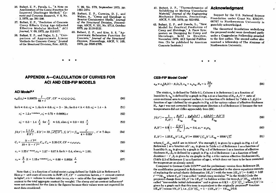
36. Babnt, Z. P., Panula, L., "A Note on Amelioration of the Creep Function fur Improved Dischinger Method," Ce­ment and Concrete Research, V. 8, No. 3,1978, pp. 381-386.

37. Bafant, Z. P., "Prediction of Concrete . Creep Effects Using Age-Adjusted

Effective Modulus Method," ACI Journal, V. 69, 1972, pp. 212-217.

38. Babnt, Z. P., and Najjar, L. J., "Com­parison of Approximate Linear Methods fur Concrete Creep," Journal of the Structural Division, Proc. ASCE,

V. 99, No. S1'9, September 1973, pp. 1851-1874.

39. Bafant, Z. P., Carreira, D. J., and Walser, A., "Creep and Shrinkage in Reactor Containment Shells," Journal of the Structural Division, Proceed­ings, ASCE, V. 101, No. STlO, October 1975, pp. 2118-2131.

40. Bazant, Z. P., and Kim, S. S, "Ap­proximate Relaxation Function for Concrete," Journal of the Structural Division, Proceedings, ASCE, V. 105, 1979, pp. 2695-2705.

* * *

APPENDIX A-CALCULATION OF CURVES FOR ACI AND CEB-FIP MODELS

ACI Model2,3

for h ... 0.4: c~ = 1; for h;;. 0.8: c~ = 3 - 3h; for 0.4 < h < 0.8: c~ = 1.4 - h

c~ = 1.2e-O.0413V'·,c~ = 0.75+ 0.00061c

c~ = 0.3 - 1.4 .!.- for'!'- ... 0.5, else c~ = 0.9 - 0.2 s a a a

J (t,t') = lE+(t?)' , E (t') = 33 ~ p3f~ (t' ), f~ (t') = f~'J8 t' , t' ;;. 7 days 4 + O.85t'

(t - t' )0.8 C, = C u, C u = 2.35 CF, CF = C1CIC3C.

10 + (t - t' )0.8

c1 = 1.25 t'-0.118; Cz = 1.27- 0.67 h forh> 0.4, elsecz = 1.00;

C3 = ~ (1 + 1.13 e-o.mv,,), c. = 0.88 + 0.0024 s 3 a

(50)

(51)

(52)

(53)

(54)

(55)

(56)

(57)

Note that c; is a function of initial moist curing defined by Table 2.8 in Reference 3. Here p = unit mass of concrete in Iblft3; CF, CF' = correction factors, c = cement content in kg/m3 , vis = volume to surface ratio in em, sla = ratio of the frne aggregate (sand) content to the total aggregate content (by weight). The slump and air content influences3

were not considered for the data in the figures because their values were not reported for most data considered.

41. Baiant, Z. P., "Thermodynamics of Solidifying or Melting Viscoelastic Material," Journal of the Engineering Mechanics Division, Proceedings, ASCE, V. 105, 1979, pp. 933-952.

42. Babnt, Z. P., and Panula, L., "New Model for Practical Prediction of Creep and Shrinkage," A. Pauw Sym­posium on Designing for Creep and Shrinkage, held in Houston, November 1978, ACI Special Publica­tion. (To be published by American Concrete Institute.)

Acknowledgment

Support by the U.S. National Science Foundation under Grant No. ENG77-06767 to Northwestern University is gratefully acknowledged.

The theoretical foundations underlying the proposed model were developed partly under a Guggenheim Fellowship awarded to the first author. The second author also received a fellowship of The Alumnae of Northwestern University.

* * *

CEB-FIP Model Code1

(58)

The strain €'t is defined by Table 0.1, Column 4 in Reference 1 as a function of humidity h; € is defined by a graph in Fig. e.4 as a function of H 0; A.IU = ratio of cross-section;3 area to exposed surface; A is a function ofh defined by Table e.l; Il.(t) = function of age t defined by six graphs in Fig. e.6 for various values of effective thickness Ho. Age t was not corrected for temperature (Section e.5 of Reference 1) because the test temperatures did not differ appreciably from 2OC.

wheref: ,E. andE are in N/mmz. The strengthf~ is given by a graph in Fig. e.l of Referen~ 1 a:; a function of t'; 'PI. is given in Table e.l of Reference 1 as a function of humidity h; 'PI. is given by a grapb in Fig. e.2 of Reference 1 as a function of effective

I thicknessHo;ll" is defined by a graph in Fig. e.3 of Reference 1 as a function ofload

(59)

(60)

(61)

duration t - t' ,Ill is given by six graphs in Fig. e.4 for various effective thicknesses H 0

(Table 2.3 of Reference 1) as a function of age t, which does not have to be here corrected fur temperature as already noted.

Compared to German Code DIN33.34 and the preliminary version from Reference 35, the modification proposed in Reference 36 and embodied in the above equations consists of replacing the actual elastic deformation IIE.(t') with the term l/E Ic (t') = 0.46(1 + 3.22 t'-o .• )/E where EIc(t') was called "initial creep modulus."29 In the Model Code the propose'rchange from IIE.(t') to IIE Ic (t') is hidden within the termlla(t' )/E':2s which is called "irreversible initial defurmation" and is given as 0.8[1 - f: (t' )If~.,] wheref; (t') is given by a graph such that this term is equivalent to the originally proposed38 function liE Ic(t' ) minus IIE.(t'), i.e.,!; (t' )If:., = 1 - [lIE Ic(t') - IIE lczs ]/0.8.

APPENDIX B-NOTATION

alc = aggregate-cement ratio (by weight) Co(t,t') = unit basic creep strain (in excess

ofl/Eo, not liE) C 1 (to) = drying diffusivity otnearly

saturated concrete at reference temperature T. at age t

C a(t,t' ,to) = increase of creep during drying

D = effective cross-section thickness E = Young's modulus of concrete Eu = E att' = 28 days E. = asymptotic modulus of concrete f: = 28-day cylinder strength of concrete gls = gravel-sand ratio (by weight) h = relative humidity of the environment

(0.;; h.;; 1) J (t,t' ) = strain at time t caused by a unit

sustained uniaxial stress acting since time t'

kA = humidity coefficient k;. = humidity coefficient ks = shape factor m = material parameter n = material parameter r = parameter

*

Discussion of this paper is invited. Please submit your comments to

*

s bv Januarv 1. 1981.

RH = relative humidity (in percent) sla = sand-aggregate ratio (by weight) sic = sand-cement ratio (by weight) S (i) = function giving shape of shrinkage

curve S a(t,t' ) = shrinkage-like time shape

function for increase of creep due to drying

t = time in days representing the age of concrete

t' = age of concrete at loading in days to = age of concrete when drying begins t = duration of drying vis = volume-to-surface ratio wlc = water-cement ratio y = parameter z = parameter a = material parameter €'A(i,t.) = shrinkage strain €,1to. = ultimate shrinkage (at zero

humidity) T.A = shrinkage square half time '1'1 = material parameter 'l'a = material parameter ~ = coefficient characterizing the increase

due to drying

*