Chaotic dynamics in the planar gravitational many-body problem

with rigid body rotations

James A. Kwiecinski, Attila Kovacs, Andrew L. Krause,Ferran Brosa Planella, Robert A. Van Gorder

Mathematical Institute, University of Oxford, Andrew Wiles BuildingRadcliffe Observatory Quarter, Woodstock Road, Oxford, OX2 6GG, United Kingdom

Robert.VanGorder@maths.ox.ac.uk

May 30, 2018

Abstract

The discovery of Pluto’s small moons in the last decade brought attention to the dynamics of thedwarf planet’s satellites. With such systems in mind, we study a planar N -body system in which all thebodies are point masses, except for a single rigid body. We then present a reduced model consisting ofa planar N -body problem with the rigid body treated as a 1D continuum (i.e. the body is treated as arod with an arbitrary mass distribution). Such a model provides a good approximation to highly asym-metric geometries, such as the recently observed interstellar asteroid ’Oumuamua, but is also amenableto analysis. We analytically demonstrate the existence of homoclinic chaos in the case where one of theorbits is nearly circular by way of the Melnikov method, and give numerical evidence for chaos when theorbits are more complicated. We show that the extent of chaos in parameter space is strongly tied tothe deviations from a purely circular orbit. These results suggest that chaos is ubiquitous in many-bodyproblems when one or more of the rigid bodies exhibits non-spherical and highly asymmetric geometries.The excitation of chaotic rotations does not appear to require tidal dissipation, obliquity variation, ororbital resonance. Such dynamics give a possible explanation for routes to chaotic dynamics observed inN -body systems such as the Pluto system where some of the bodies are highly non-spherical.

keywords: celestial mechanics; many body problem; rigid bodies; chaotic dynamics; Melnikov method

1 Introduction

The study of N -body problems, whereby the bodies are treated as point masses, has a long and storiedhistory Musielak & Quarles (2014). There has been much effort on finding new orbits to the planar three-body problem, with a large number of new orbits found over the last few decades Moore (1993); Chenciner& Montgomery (2000); Nauenberg (2001); Chenciner et al. (2005); Nauenberg (2007); Dmitrasinovic &Suvakov (2015). In particular, very recent work has uncovered hundreds of new orbits in the planar three-body problem Suvakov & Dmitrasinovic (2013); Li & Liao (2017); Dmitrasinovic et al. (2017). In all suchstudies, one assumes that each mass is a point mass. There is also work done on the statistical mechanicsof N -body problems Lynden-Bell (1995); Lynden-Bell & Lynden-Bell (1999) as well as extensions to therelativistic regime Eddington & Clark (1938).

In contrast to the N -body problem for point masses, there have been relatively fewer studies on orbitaldynamics when the masses are rigid bodies. There have been a number of recent studies on the rotation ofrigid bodies Lara (2014); Hou et al. (2017); Boue (2017). It was recently shown that a relative equilibriummotion of N ≥ 3 disjoint rigid bodies is never an energy minimizer Moeckel (2017), a generalization of aknown result about point masses in the N ≥ 3 body problem Moeckel (1990) to the case of rigid bodies.

Rigid body dynamics are of great relevance to applications in celestial mechanics when a mass is non-spherical. Small bodies with diameters smaller than 1000 km usually have irregular shapes, often resemblingdumbbells or contact binaries Melnikov & Shevchenko (2010); Jorda et al. (2016); Lages et al. (2017). The

1

arX

iv:1

801.

0245

8v2

[as

tro-

ph.E

P] 2

9 M

ay 2

018

spinning of such a gravitating dumbbell creates a zone of chaotic orbits around it Mysen et al. (2006);Frouard & Compere (2012); Mysen (2009), and these dynamics were recently studied in Lages et al. (2017),where it was shown that the chaotic zone increases in size if the rotation rate is decreased. To do so, Lageset al. (2017) generalized the Kepler map technique Meiss (1992) to describe the motion of a particle in thegravitational field of a such a rotating irregular body modeled by a dumbbell. Regarding the rotations of suchan irregular object itself, Fernandez-Martınez et al. (2016) recently studied dynamics from planar oscillationsof a dumbbell satellite orbiting an oblate body of much larger mass, obtaining a kind of generalized Beletskyequation. They show the existence of chaotic orbits in their system via the Melnikov method, and studythe transition between regular to chaotic orbits numerically through the use of Poincare maps. The modelstudied was originally derived in Abouelmagd et al. (2015), and while interesting, is fairly restrictive on thegeometry and mass distribution in the rigid body, while further assuming that the satellite body is of muchsmaller mass to the oblate body it orbits.

One of the large astronomical bodies to first get attention for its possible chaotic motion was Hyperion,a highly non-spherical moon of Saturn. In Wisdom et al. (1984), the authors analyze the spin-orbit couplingof Hyperion, modeled as a homogeneous ellipsoid orbiting around a point mass, to determine the criticaloblateness of the ellipsoid that induces chaos in the system. They conclude their analysis with a predictionof chaotic tumbling for Hyperion. Later, Tarnopolski (2017b) further studied the motion of oblate satellitesand applied the results to Hyperion as well. A control term was introduced to the Hamiltonian of the systemin order to reduce the chaotic behavior; numerical simulations showed that the control term manages toeffectively reduce the chaotic behavior of the system and, for some parameter values, it even succeeds insuppressing chaos. On the other hand, Tarnopolski (2017a) studied the effect of a second satellite in thedynamics of an oblate moon, applied in particular to the effects of Titan in the Saturn-Hyperion system.Building up from the model used in Wisdom et al. (1984), Tarnopolski introduces a second satellite as apoint mass. The numerical simulations of the model show how the presence of a second satellite can resultin a transition of periodic orbits into chaos. Instead of spin-orbit coupling, spin-spin coupling is presentedin Batygin & Morbidelli (2015) and is studied in a system formed by a non-spherical satellite of negligiblemass (modeled as a dumbbell) orbiting around a non-spherical mass distribution (modeled as an ellipsoid).The analysis on the asteroidal systems (87) Sylvia and (216) Kleopatra show spin-spin resonances but thereis no evidence of chaos in their motions.

The discovery of Pluto’s small moons in the last decade has resulted in much attention directed tounderstanding the dynamics of Pluto’s satellites. The four small moons (Styx, Nix, Kerberos, and Hydra)orbit around the binary system formed by Pluto and its largest moon, Charon. Showalter & Hamilton(2015) looked for resonances in the orbits of Pluto’s small moons and they found that the Pluto-Charonsystem appears to induce chaos in non-spherical moons without the need of resonance, which was not seen inother well studied three-body systems such as Saturn-Titan-Hyperion. In particular, Showalter & Hamilton(2015) conjectured that non-spherical moons may rotate chaotically with no resonance required. An orbitclassification on the Pluto-Charon system is provided in Zotos (2015), in which the author, using numericalsimulations on the gravitational potential generated by the binary system, distinguishes three types of orbits(bounded, escaping, and collisional) depending on their initial conditions. In Correia et al. (2015), the spin-orbit coupling for a non-spherical satellite orbiting around a binary system was studied, with a particularapplication to the small moons of the Pluto-Charon system. Their numerical simulations show chaoticbehavior for the small moons of Pluto. In particular, a dynamical mechanism for the chaotic behavior wasproposed by Correia et al. (2015) who showed that for slowly spinning satellites, spin-binary resonancesfrom Charon’s periodic perturbations are sufficiently strong to cause chaotic tumbling. Finally, in Jianget al. (2016), the authors study the N -body problem for irregular bodies, including gravitational, electric,and magnetic fields. They present numerical simulations on several N -body systems, with the full six-bodyPluto’s system among them.

Recent New Horizons observations showed that the low mass satellites are spinning faster than consideredby Showalter & Hamilton (2015); Correia et al. (2015), with angular spin rates many times greater than theirorbital mean motions, implying that despinning due to tidal dissipation has not taken place Weaver et al.(2016). At higher spin states, spin-orbit and spin-binary resonances may not be as strong, so chaoticallytumbling is not assured. In Quillen et al. (2017), the authors used a damped mass-spring model within an N -body simulation to study spin and obliquity evolution for single spinning non-round bodies in circumbinaryorbit. Their simulations with tidal dissipation alone do not show strong obliquity variations from tidally

2

induced spin-orbit resonance crossing and this was attributed to the high satellite spin rates and low orbitaleccentricities. However, a tidally evolving Styx does exhibit intermittent obliquity variations and episodesof tumbling. As stated in Quillen et al. (2017), “We lack simple dynamical models for phenomena seen inour simulations, such as excitation of tumbling.”

With such applications in mind, we will consider an N -body system in which all of the bodies are pointmasses, except for a single body which has finite size. We then present a reduced model which considers thebody as a 1D geometry. The body is treated as a rod with an arbitrary mass distribution in this simplifiedmodel. This model contrasts with other work which consider the gravitational field as a perturbation from aperfect sphere (i.e. ellipticity close to zero), such as the work presented in Correia et al. (2014); Delisle et al.(2017). Our 1D rod model is highly asymmetric, equivalent to an ellipticity of unity, and is an approximationfor celestial bodies such as the interstellar asteroid ‘Oumuamua which was recently observed Meech & et al.(2017). Additionally, our rotational equation of motion for the 1D rod is valid for non-Keplerian orbitswhich is in contrast with the Beletsky equation Beletskii (1966); Celletti (2010) for the rotation of dumbbellsystems, of which our model can be considered as a continuum limit.

The translational motion equations in our model are equivalent to the N -body problem for point masseswhilst an additional rotational motion equation, arising from tidal corrections to the gravitational force, isincluded for the rigid body. Thus, if orbits are known, they can be fed into the rotational motion equationwhich can then be solved. The rotational motion equation only depends on the positions of the other pointmasses. Note that since the translational motion equations do not depend on the angles or inertial terms ofthe rigid body, chaos in the rotational motion of one or more bodies will not result in chaotic trajectories ofthe orbits themselves. Such dynamics give a possible explanation for the route to chaotic dynamics observedin N -body systems such as the Pluto system. Our results here emphasize that tidal dissipation, obliquityvariation, and orbital resonances are not required for the existence of chaotic rotations in the simple planarsetting. These results suggest generic chaotic rotation of non-spherical moons in more realistic settings, asconjectured by Showalter & Hamilton (2015).

The rest of the paper is organized as follows: In Section 2, we shall describe the simplified model ofthe N -body problem including rotation of a single rigid body which has a 1D geometry. In Section 3, weapply the Melnikov method in order to analytically demonstrate the emergence of homoclinic chaos in therotational motion equation under perturbations of approximately circular orbits. This analytical approachrequires the construction of homoclinic connections which is possible in fairly restricted cases, such as thatof the circular orbit. Therefore to consider more complicated orbits, we provide numerical simulations andconsider resulting time series and Poincare sections in Section 4 to demonstrate the existence of chaoticdynamics in the rotational motion of the rigid bodies under perturbations of more complicated orbits, suchas the well-known figure-8 orbit. Such results suggest that chaos from perturbations of orbits in the N -bodyproblem (N ≥ 2) for a rigid body is ubiquitous. We summarize and discuss the results in Section 5.

2 Planar orbital dynamical system of a single rotating rod

We study a system of N bodies that exert gravitational forces on each other, with N − 1 point masses anda single rigid body of finite geometry, which we will refer to as the Nth body hereafter. In particular, weconsider a rigid body in the shape of a 1D rod. We view this as a proxy for a more general asymmetricbody whose geometry deviates largely from the sphere, but allows for a number of analytical simplifications,permitting later analysis of the dynamics. The orbital dynamics are taken to be planar as this both simplifiesthe mathematics yet still agrees with many real orbital systems, such as the Pluto system. Additionally,instability in the planar setting suggests instability in the full problem as there are more degrees of freedom.

We suppose the motion, both translational and rotational, of the bodies is confined to the x-y inertialplane and we do not assume that the orbit is necessarily Keplerian. We denote the position of the ith body’scenter of mass by the vector ri = (xi, yi) and the orientation of the Nth rigid rod with respect to the positivex-axis as the angle θ. The equations of orbital motion and additional rotation due to the gravitational fieldgenerated by the N bodies, which are separated on a length-scale that is much larger than the size of the

3

rigid rod, is given by (see Appendix A for details)

d2xidt2

=∑j 6=i

Gmj (xj − xi){(xj − xi)2 + (yj − yi)2

}3/2, (1)

d2yidt2

=∑j 6=i

Gmj (yj − yi){(xj − xi)2 + (yj − yi)2

}3/2, (2)

for i = 1, 2, . . . , N , and

d2θ

dt2=

3G

2

N−1∑j=1

mj

(2 (xj − xN ) (yj − yN ) cos 2θ +

[(yj − yN )

2 − (xj − xN )2]

sin 2θ)

((xj − xN )

2+ (yj − yN )

2)5/2 . (3)

Scaling the angular variable as θ = 2θ and then dropping hats, we have that the rotational variable θevolves via a non-autonomous ODE of the form

d2θ

dt2= F1(t) cos θ − F2(t) sin θ, (4)

where

F1(t) =

N−1∑j=1

6Gmj (xj − xN ) (yj − yN ){(xj − xN )

2+ (yj − yN )

2}5/2

, (5)

and

F2(t) =

N−1∑j=1

3Gmj

[(yj − yN )

2 − (xj − xN )2]

{(xj − xN )

2+ (yj − yN )

2}5/2

. (6)

We comment on some important aspects of (1)-(3). First, the translational dynamics of all masses inthe system are given by the point approximation which is a consequence of the rigid body having a highlyasymmetric geometry that is very small compared to the separations of all the bodies. In particular, thequadrupole or first order corrections to the gravitational field generated and felt by the Nth rigid bodyvanish. This aspect contrasts with other models which consider the bodies as perturbations from perfectspheres, such as the work presented in Correia et al. (2014) where such corrections are non-trivial in theorbital dynamics. Other instances where the higher order terms are non-negligible include the oppositeregime considered here where the bodies are no longer well separated with respect to their size Delisle et al.(2017).

Second, the rotational equation of motion (3) is valid for non-Keplerian orbits which is in contrast withthe Beletsky equation Beletskii (1966); Celletti (2010) for the rotation of dumbbell systems. Note that thisdumbbell system is a singular limit of our model presented here. However, in our case the angular equationcompletely decouples from the translational equations, meaning that the 2N translational equations can besolved and their solutions placed into the rotation equation.

3 Application of the Melnikov method for homoclinic chaos

We consider the Melnikov method Mel’nikov (1963); Arnold (1964); Guckenheimer & Holmes (2013); Wiggins(2003) in order to show that system (1)-(3) admits homoclinic chaos, as the method is used to understandchaos resulting from nonintegrable perturbations of Hamiltonian systems Holmes & Marsden (1982b,a);Camassa et al. (1998); Yagasaki (1999). We note that (1)-(3) is of this near-integrable form, with thedominant integrable part comprising of the orbital dynamics of the point masses and the constant rotation ofthe rigid body, given that the tidal forces vanish to leading order. The nonintegrable part of the Hamiltoniancomes from the gravitational torque applied to the body, specifically for orbits which are non-circular as will

4

be shown, similar to the Beletsky equation for non-zero orbit eccentricity Burov (1984); Celletii & Sidorendko(2008). The approach has been used to find homoclinic or heteroclinic chaos in a variety of systems Lin(1990); Hogan (1992); Yagasaki (1994); Spyrou & Thompson (2000); Zhang et al. (2009, 2010) and has alsobeen used to assist in the control of such chaos Chacon (2006). The method has been applied to homoclinicorbits corresponding to elliptic functions Belhaq et al. (2000). The approach has also been used in thestudy of nonlinear PDEs, such as a reduction of the perturbed KdV equation Grimshaw & Tian (1994). Ofimmediate relevance to our problem, in addition to the recent application to the dumbbell satellite problemFernandez-Martınez et al. (2016), the method has been applied to restricted three-body problems Xia (1992).

We show that chaos occurs in a system consisting of a circular orbit perturbed under small deformations.To do so, we apply Melnikov’s method, which can be used to prove the existence of transverse homoclinicorbits in the non-autonomous dynamical system

u = f (u) + ηg (u, t) , (7)

for η sufficiently small. In our setting, (7) is the first-order form of the second order equation (3). Note thatthis method is valid for non-automonous perturbations which are periodic Mel’nikov (1963), quasiperiodicWiggins (1987), and random Lu & Wang (2010) and there is no assumption made as to the frequency ofsuch perturbations.

The quantity of interest is the Melnikov function, which takes the form

M (t0) =

∞∫−∞

f(u(0) (t)

)∧ g

(u(0) (t) , t+ t0

)dt, (8)

where u(0) (t) is the explicit form of a homoclinic orbit for η = 0 in (7), t0 ∈ R, and f ∧ g = f1g2 − f2g1.The Melnikov function quantifies the distance between unstable and stable manifolds, so if there existsa t0 such that there is a simple zero of M (t0), then transverse homoclinic orbits exist in the dynamicalsystem. Furthermore, such trajectories imply the existence of a Smale horseshoe and, by extension, chaosGuckenheimer & Holmes (2013).

For the present analysis, we study the planar rotation of a single body, which, in its simplest form, isdescribed by the non-automonous system

d2θ

dt2= F1 (t) cos θ − F2 (t) sin θ, (9)

where F1 (t) and F2 (t) (as given in (5)-(6)) are forces acting on the rod and will generally depend on time.

3.1 Purely circular orbit and forcing

Consider the case where the orbit of the Nth rigid body is circular, while the other orbits are small relativeto this circular orbit. Mathematically, we write xN = −A cos(γt/2), yN = −A sin(γt/2), with xj = AδPj(t)and yj = AδQj(t) for periodic Pj(t), Qj(t) and δ << 1 for all j = 1, 2, . . . , N − 1. Here γ > 0 is a parameterrelated to the period of the orbit. Taking these in (3) and applying multiple-angle trigonometric identities,we then have

d2θ

dt2= σ(sin(γt) cos(θ)− cos(γt) sin(θ))

+3σδ

2sin(θ)

N−1∑j=1

mj {(5 cos(3γt/2) + cos(γt/2))Pj(t)

+(5 sin(3γt/2)− sin(γt/2))Qj(t)}

+3σδ

2cos(θ)

N−1∑j=1

mj {(5 cos(3γt/2)− cos(γt/2))Qj(t)

−(5 sin(3γt/2) + sin(γt/2))Pj(t)}+O(δ2) ,

(10)

5

where

σ =3(N − 1)G

A3. (11)

From the above derivation, if the orbit of the rotating rod is purely circular, then the forces in the x andy direction will be sinusoidally periodic with a non-zero angular frequency γ such that their explicit form is

F =

(FxFy

)= σ

(cos(γt)sin(γt)

), (12)

up to lowest order (neglecting O(δ) corrections). The rotation of the rod then evolves according to thenon-autonomous ODE

d2θ

dt2= sin(γt) cos(θ)− cos(γt) sin(θ) = − sin (θ − γt) , (13)

where the time and angular frequency have been rescaled as t→ t√σ and γ

√σ → γ. Making the change of

variable θ = θ−γt, which relates the old and new angular variable by a constant rotation of angular velocityγ, we find that (13) reduces to

d2θ

dt2= − sin θ, (14)

which is an automonous system in θ. This result implies that no aperiodicity will occur in θ and, as such, arod cannot exhibit chaotic rotation if it is in a purely circular orbit.

We note that (14) has exactly one homoclinic orbit, given the periodic domain in θ ∈ (−π, π]. Todetermine its form, we multiply (14) through by dθ/dt and integrate with respect to t to obtain

1

2

(dθ

dt

)2

+ V(θ)

= E, (15)

where E is a constant analogous to the total mechanical energy of the rotating rod in a potential V(θ)

=

− cos θ. The homoclinic orbit connects the fixed point at θ = π along the level set E = 1, so the homoclinicorbit in θ(0) is found by solving

dθ(0)

dt= ±

√2(

1 + cos θ(0)), (16)

for the initial condition θ(0) (t = 0) = 0. Using a double angle formula, dθ(0)

dt = ±2 cos(θ/2)

, and, by

introducing a rescaling θ(0)/2 → φ(0), we obtain, by separation of variables, ln∣∣secφ(0) + tanφ(0)

∣∣ = ±t,having imposed the initial condition φ(0) (t = 0) = 0. Rearranging to find an explicit form for φ(0), secφ(0) +tanφ(0) = exp (±t). We simplify this expression to tanφ(0) = 1

2 {exp (±t)− exp (∓t)}, which results in thetime explicit angular position

θ(0) (t) = ±2 tan−1 (sinh (t)) . (17)

Note that tan−1 (t) is an odd function, and that (17) approaches ±π as t → ±∞ for the positive solution,and the opposite sign for the negative solution. By differentiating with respect to time, we find the timeexplicit angular velocity

d

dtθ(0) = ±2sech (t) . (18)

3.2 Perturbations of the circular forcing

We now consider an arbitrary number of periodic perturbations to the circular orbit which are of O (η) suchthat δ � η � 1. Explicitly, suppose that the force exerted on the rod takes the form

F = σ

(cos(γt)sin(γt)

)+ ση

(F11(t)F2(t)

), (19)

6

where F1,F2 are bounded and C1(R) perturbations. We shall assume that such perturbations are oscillatoryabout zero (including periodic or quasi-periodic perturbations) and in practice write(

F1(t)F2(t)

)=

∞∑k=1

(αk sin(kpt) + βk cos(kpt)

αk sin(kpt) + βk cos(kpt)

), (20)

where the coefficients αk, βk, αk, and βk are O(1) in and p > 0 is a constant. The perturbation angularfrequencies p ∈ R need not necessarily be integer multiples of γ or even rational multiples, allowing us toconsider not only periodic but also quasi-periodic orbits with precession, provided η � 1 holds. In the caseof periodic forcing, the series will terminate at some maximal index k, resulting in finite sums. In the quasi-periodic forcing case, infinitely many terms would be needed, and one should ensure that the perturbationseries do converge in such cases. For our interests, we shall consider only perturbations with convergentFourier series.

The non-autonomous evolution of the angular position then reads

d2θ

dt2= − sin (θ − γt) + η cos θ

∞∑k=1

{αk sin(kpt) + βk cos(kpt)

}− η sin θ

∞∑k=1

{αk sin(kpt) + βk cos(kpt)} ,(21)

where we have rescaled time as t→ t√σ and p

√σ → p. Making the change of variables θ = θ− γt, applying

trigonometric rules, and assuming the necessary results on the convergence of the series, we obtain

d2θ

dt2= − sin

(θ)

+η

2

∞∑k=1

{(αk − βk) sin

(θ + (γ + kp) t

)− (αk + βk) sin

(θ + (γ − kp) t

)+(βk + αk) cos

(θ + (γ + kp) t

)+ (βk − αk) cos

(θ + (γ − kp) t

)}.

(22)

In the particular case of (22), equation (8) becomes

M (t0) =1

2

∞∫−∞

d

dt

(θ(0) (t)

) ∞∑k=1

{(βk + αk) cos

(θ(0) + (γ + kp) (t+ t0)

)+ (βk − αk) cos

(θ(0) + (γ − kp) (t+ t0)

)+ (αk − βk) sin

(θ(0) + (γ + kp) (t+ t0)

)−(αk + βk) sin

(θ(0) + (γ − kp) (t+ t0)

)}dt,

(23)

where θ(0) (t) and dθ(0)

dt are the explicit homoclinic orbits of the rescaled angular position and velocity in thepurely circular system (14).

Using (17) and (18) in the particular Melnikov function (23) and performing the integration, we obtain

M (t0) = ±∞∑k=1

{µk,+(βk + αk) cos [(γ + kp) t0] + µk,−(βk − αk) cos [(γ − kp) t0]

+µk,+(αk − βk) sin [(γ + kp) t0]− µk,−(αk + βk) sin [(γ − kq) t0]} ,(24)

whereµk,± = π (γ ± kp)2

{sech

[π2

(γ ± kp)]− csch

[π2

(γ ± kp)]}

. (25)

7

Recall that we assume F1,F2 are bounded and C1(R) perturbations which are oscillatory about zero.Define

µ(χ) = πχ2{

sech[πχ

2

]− csch

[πχ2

]}, (26)

and note that µ(0) = 0, exp(|χ|)µ(χ) → 0 as χ → ±∞, and |µ(χ)| < µ ≈ 2.76 for all χ ∈ R, where thisvalue comes from extremizing (26). Therefore, µk,± = 0 if and only if γ ± kp = 0, and the sequences µk,±are bounded and decay for large enough k (with the decay rate being faster than exponential).

Manipulating the series in (24), we find that

M (t0) = − sin(γt0)

∞∑k=1

(µk,+ + µk,−) (αk sin(kpt0) + βk cos(kpt0))

+ cos(γt0)

∞∑k=1

(µk,+ − µk,−

kp

)(αk sin(kpt0) + βk cos(kpt0))

′

+ cos(γt0)

∞∑k=1

(µk,+ + µk,−)(αk sin(kpt0) + βk cos(kpt0)

)− sin(γt0)

∞∑k=1

(µk,+ − µk,−

kp

)(αk sin(kpt0) + βk cos(kpt0)

)′,

(27)

and recalling the definitions of F1,F2, we see that M(t0) involves terms which are scalings of the terms inF1,F2 and their derivatives. Due to the properties of µ(χ) listed above, we have that

|M(t0)| ≤ 2

(maxχ

µ(χ)

)maxt∈R

{|F1(t)|+ 1

p|F ′1(t)|+ |F2(t)|+ 1

p|F ′2(t)|

}≤ 2µmax

t∈R

{|F1(t)|+ 1

p|F ′1(t)|+ |F2(t)|+ 1

p|F ′2(t)|

}.

(28)

As p is positive and finite, and F1,F2 are bounded with bounded derivatives, then the function M(t0)is bounded in t0. Since F1,F2 are oscillatory about zero, so are their derivatives. Then either M(t0) isoscillatory about zero or it is a constant. The only possible constant value is zero, and if this occurs thenM(t0) is identically zero and we have no simple zeros.

Note that for γ, p > 0, then at most one of µk,+, µk,− can be zero. If there is more than one term in theperturbation expansion, then there will always be at least one non-zero coefficient of a sine or cosine term,and hence M(t0) will have countably many simple zeros. If there is exactly one term in each perturbation

expansion, then M(t0) will have countably many simple zeroes unless γ = −p, β1 = α1, α1 = −β1 or γ = p,

β1 = −α1, α1 = β1 (where, without loss of generality, k = 1 in a one-term perturbation expansion).Therefore, excluding such a narrow class of perturbations, the function M(t0) is not identically zero

and oscillates about zero. As such, there exist countably infinitely many values of t0 ∈ R for which simplezeros will occur regardless of the values for γ, again provided that the coefficients of (24) are not such thatM(t0) ≡ 0. By the Melnikov criteria, transverse homoclinic orbits exist in the perturbed periodic system forη � 1 under such conditions.

These results suggest that the physical parameters associated with the orbital dynamics and the rotationaldynamics are irrelevant. The only necessary requirement for chaos is that the gravitational torque exertedon the rigid body is non-zero. Note however that this result only shows the existence of chaotic rotation inthe system, and not the extent to which it occurs. For example, rotational periodic motions may still bepossible Levin (1993); Celletii & Sidorendko (2008).

4 Numerical simulations and verification of chaos

While the results obtained from the Melnikov method demonstrate that chaos should be ubiquitous due toarbitrary small perturbations of circular orbits, for more complicated orbits the analytical method is nottractable. As such, we shall consider numerical simulations in order to demonstrate chaotic dynamics in

8

-1.5 -1 -0.5 0 0.5

-1

-0.5

0

0.5

1

Figure 1: The plot on the left depicts four different circular orbits for the rigid rod around a massive bodywith initial perturbations of y1(0) = 0, 0.1, 0.3, and 0.5 leading to successively larger circular orbits that areto the left of the massive body (which remains approximately fixed independent of the perturbation). Theplot on the right is of a figure-8 orbit with three bodies of identical masses.

a variety of other orbital configurations, which suggests that chaotic rotations should be quite common inplanar N -body dynamics. We shall begin by showing that the numerical simulations agree with the Melnikovanalysis in the case of a single nearly circular orbit, in order to verify the numerical approach against ouranalytical results. Our focus then shifts to three bodies in more complicated orbital configurations, whichsuggests that the results are robust for N -body dynamics.

We now demonstrate numerical simulations of rotating rigid bodies within sample orbital simulations,and discuss the transition to chaotic dynamics observed. We study two examples in detail: perturbed circularorbits in a two-body system, and the figure-8 orbit of the three body system. Both of these orbits are shownin Fig. 1. The simulations were implemented using the Matlab function ode113 with relative and absolutetolerances set to 2.22045 × 10−14. We also performed the same simulations using an 8-stage Runge-Kuttascheme due to Papakostas & Tsitouras (1999) in Matlab, as well as in Mathematica using the functionNDSolve and found consistent results using all three methods for all simulations shown.

4.1 Simulations for perturbed circular orbits

To generate our circular orbits in the two-body case we set G = 1, m1 = 1, and m2 = 10−13 so that the secondbody will have a negligible effect on the first, which will be stationary to within an approximately-circularorbit of size O(10−13). We set x2(0) = 0, y2(0) = 1, x1(0) = 0, y1(0) = 0, x2(0) = −(m2

1/(m1+m2))1/2 ≈ −1,x1(0) = −x2(0), y1(0) = 0, and vary y2(0) as a perturbation or bifurcation parameter. We simulate thesystem for T = 300 units of time corresponding to ≈ 550 orbits (which depends on the perturbed orbit).

In Fig. 2 we plot some simulations of the rotation of the small body as it orbits around the larger one.We see that for a perfectly circular orbit, the body rotates primarily in one direction with some ‘wobble’due to the orbital forcing. The angular velocity reveals this to just be integrated periodic motion, and soit is also periodic (modulo the period). As the velocity perturbation is increased, multiple-frequency effectsare observed in the angular velocity, and these correspond to variations in the wobbling previously seen atintermittent intervals. Finally for large enough perturbations, these small irregularities begin to occur morefrequently, and the angular position of the body becomes increasingly unpredictable. These behaviours aregeneric throughout the portions of the phase space that we explored.

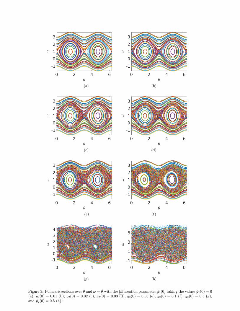
We construct a Poincare section for this system by considering the times Tp = {t ∈ R : x2(t) = 0, x2(t) >0} corresponding to the bottom of the orbit in Fig. 1. We vary the initial angle θ(0) from 0 to 2π in 10increments, and the initial angular velocities θ(0) = ω(0) from −1 to 3 in 10 increments, and plot values ofω(t) against θ(t) mod 2π for t ∈ Tp in Fig. 3.

For no perturbation, we see only periodic orbits, corresponding to rotation that ‘wobbles’ in its orbit with

9

0 10 20 30

-12

-10

-8

-6

-4

-2

0

0 10 20 30

-0.8

-0.6

-0.4

-0.2

0

(a) (b)

0 10 20 30

-12

-10

-8

-6

-4

-2

0

0 10 20 30

-1

-0.8

-0.6

-0.4

-0.2

0

(c) (d)

0 50 100

-30

-20

-10

0

0 50 100

-1

-0.5

0

0.5

(e) (f)

Figure 2: Time series for the perturbed circular orbit showing θ(t) and ω(t) = θ(t) with both initially set toθ(0) = ω(0) = 0 for y2(0) = 0 (a)-(b), y2(0) = 0.1 (c)-(d), and y2(0) = 0.5 (e)-(f) in each case.

10

(a) (b)

(c) (d)

(e) (f)

(g) (h)

Figure 3: Poincare sections over θ and ω = θ with the bifurcation parameter y2(0) taking the values y2(0) = 0(a), y2(0) = 0.01 (b), y2(0) = 0.02 (c), y2(0) = 0.03 (d), y2(0) = 0.05 (e), y2(0) = 0.1 (f), y2(0) = 0.3 (g),and y2(0) = 0.5 (h).

11

a periodic motion. As we perturb the orbit slightly, we see that specific orbits are destroyed due to resonancewith the slightly-perturbed orbit. Further increasing the perturbation, we see a transition to global chaoticdynamics throughout the phase space, with small islands of stability remaining by the final plot Lichtenberg& Lieberman (2013).

4.2 Simulations for perturbed figure-8 orbits

We now consider the three-body problem with a figure-8 orbit as shown in Fig. 1. All three bodies haveplanar motion along the figure-8 curve. See Chenciner & Montgomery (2000); Chenciner et al. (2005);Nauenberg (2007) for further discussion on figure-8 orbits. Given that the orbital dynamics specified forthe rigid body being a 1D rod is given by the point mass approximation to leading order, with first ordercorrections vanishing and second order corrections being negligible in the regime of the size of the rigidbody being much smaller compared to the separation of bodies in the system, the figure-8 orbit is stable asdiscussed by work in Hu & Sun (2009); Roberts (2007). For instances where the rigid body can be modelledvia perturbations to a sphere and for trajectories that approach on a length scale that is comparable in sizeto the geometry of the rigid body, such as for the models considered by Correia et al. (2014); Delisle et al.(2017), higher order terms would cause this particular periodic orbit to become unstable.

This orbit is far from circular, and hence the analytical chaos results for perturbations of circular orbitspresented in the previous section do not hold here. However, we shall still demonstrate via numericalsimulations that chaos is ubiquitous in this configuration, suggesting that the circular orbit is the specialcase where chaos does not exist.

In Fig. 4, we plot the angle and angular velocity corresponding to three different values of ω(0). Bothangular position and velocity exhibit chaotic motions. In particular the angular position θ(t) has a run-and-tumble behaviour where the body is spinning in one direction for many orbits before it begins rotating inthe opposite direction (note that for this simulation, the three-body orbit has a period T ≈ 6.3490473929,as reported in Li & Liao (2017)).

In Fig. 5 we plot a Poincare section for ω(0) = 0 using the same discretization of initial values as before,and the same definition of the Poincare section at Tp for 300 orbits. As expected, we see what appears tobe completely ergodic behaviour indicative of global Hamiltonian chaos Lichtenberg & Lieberman (2013).

The figure-8 orbits are but one example of the possible orbits for the planar three-body problem, andtherefore constitute another example where chaotic dynamics emerge in the rotational motion of the rigidbodies. We found similar results for many of the planar three-body problem orbits, recently discovered inLi & Liao (2017); Dmitrasinovic et al. (2017). This suggests that such chaos should be ubiquitous in theN -body problem where one body is non-spherical.

5 Discussion

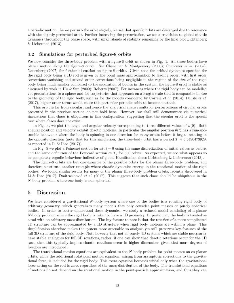
We have considered a gravitational N -body system where one of the bodies is a rotating rigid body ofarbitrary geometry, which generalizes many models that only consider point masses or purely sphericalbodies. In order to better understand these dynamics, we study a reduced model consisting of a planarN -body problem where the rigid body is taken to have a 1D geometry. In particular, the body is treated asa rod with an arbitrary mass distribution. The key feature to note is that the rotation of a more complicated3D structure can be approximated by a 1D structure when rigid body motions are within a plane. Thissimplification therefore makes the system more amenable to analysis yet still preserves key features of thefull 3D structure of the rigid body. Note however that not all purely 1D systems which are stable necessarilyhave stable analogues for full 3D rotations, rather, if one can show that chaotic rotations occur for the 1Dcase, then this typically implies chaotic rotations occur in higher dimensions given that more degrees offreedom are introduced.

The translational motion equations are equivalent to the N -body problem for point masses on co-planarorbits, while the additional rotational motion equation, arising from asymptotic corrections to the gravita-tional force, is included for the rigid body. This extra equation becomes trivial only when the gravitationalforce acting on the rod is zero, regardless of the mass distribution of the body. The translational equationsof motions do not depend on the rotational motion in the point-particle approximation, and thus they can

12

0 500 1000 1500

-1500

-1000

-500

0

500

0 500 1000 1500

-5

0

5

(a) (b)

0 500 1000 1500

-2000

-1500

-1000

-500

0

500

0 500 1000 1500

-5

0

5

(c) (d)

0 500 1000 1500

0

500

1000

1500

2000

2500

0 500 1000 1500

-5

0

5

(e) (f)

Figure 4: Time series for the figure-8 orbit showing θ(t) and ω(t) = θ(t) with θ(0) = 0, for ω(0) = 0 (a)-(b),ω(0) = 10−5 (c)-(d), and ω(0) = 1 (e)-(f).

13

Figure 5: A Poincare section over θ and ω = θ for the figure-8 orbit in Figure 1.

be solved just as for N -body problems in order to obtain the orbits. Once the orbits are determined, one canplace the rotational motion equation on top of these results, feeding the orbits as a non-autonomous forcing.

We analytically demonstrate the existence of homoclinic chaos in the case where one of the orbits isnearly circular by way of the Melnikov method, and give numerical evidence for such chaos when the orbitsare more complicated (such as more extreme elliptical orbits or figure-8 orbits). These results suggest thatchaos is ubiquitous in such N -body problems when one or more of the rigid bodies is non-spherical. We showthat the extent of chaos in parameter space is strongly tied to the deviations from purely circular orbits.Such dynamics give a possible explanation for routes to chaotic dynamics observed in many-body systemssuch as the Pluto system in which some of the bodies are better approximated as rods rather than perfectspheres.

The circular orbits and figure-8 orbits are specific examples, and due to the wide appearance of chaos inthe parameter space of these problems, we can likely find similar results for many of the planar three-bodyproblem orbits, such as those recently discovered in Dmitrasinovic et al. (2017); Li & Liao (2017). Moregenerally, since all that is required for the appearance of chaos is for one rigid body to exhibit chaoticrotations, the results naturally extend to N -bodies, in planar or non-planar (fully 3D) configurations. Thissuggests that such chaos should be ubiquitous in the N -body problem when one or more of the bodies arerigid and non-spherical.

Returning to the motivating application, recall that in the Pluto system, the asymmetric Styx does appearto exhibit intermittent obliquity variations and episodes of tumbling, suggesting some form of chaos in therotational dynamics Showalter & Hamilton (2015); Correia et al. (2015); Quillen et al. (2017). The resultswe obtain suggest that chaos could be ubiquitous in the rotational dynamics of such small moons when theyare geometrically asymmetric, given its existence in the absence of tidal dissipation, obliquity variation, andorbital resonance. This outcome could explain why Styx appears to exhibit rotational chaos or tumblingwhile other satellites or moons in the Pluto system, which are more symmetric, may not. Indeed, theemergence of such chaotic dynamics from only orbital forcing and non-sphericity of the rigid body suggeststhat such chaotic tumbling may be prevalent in many systems where some of the bodies have asymmetricgeometries.

Acknowledgments

The authors would like to thank A. Goriely for helpful and worthwhile discussions and T. G. Bollea forinspiration.

6 Appendix: Derivation of orbital mechanics for a single rigidrotating rod

We first give a general formulation of the problem of N orbiting bodies, with N−1 point masses and a singlerigid body of arbitrary shape, which we will refer to as the Nth body hereafter. We assume that the bodies

14

are separated on a length scale much larger than the geometry of the body. We then restrict our attentionto a 1D geometry for the rigid body, resulting in a single rotational equation for a rod of arbitrary massdistribution.

6.1 Rotating rigid body under gravitational forces

We study a system of N rigid bodies that exert gravitational forces on each other. The Nth body hasa reference configuration B0 ⊂ R3 initially and is mapped to a current configuration Bt ⊂ R3 at time t.The position vector rN points from an arbitrary origin to the body’s center of mass. For a rigid body, thecenter of mass occurs at the same material point in the reference configuration, however the body itself willtranslate and rotate according to the effects of gravity.

We determine the time-evolution of the translation of the point masses. In particular, we make use ofthe balance of linear momentum to obtain that the acceleration of the ith point mass at time t is

midvidt

=

N−1∑j 6=i

Gmimj

|rj − ri|3(rj − ri) +Gmi

∫Bt

ρ (Rt)

|Rt − ri|3(Rt − ri) dVt, (29)

where the integral is taken over the volume in the current configuration Bt, ρ (Rt) is the mass density of theNth continuum, Rt is the position vector of a material point in Bt, G is the universal gravitational constant,dvi

dt is the acceleration field of the ith body, and mj for j = 1 . . . N − 1 are the masses of the point masses.The mass of the Nth body is constant for all time and is given as

mN =

∫Bt

ρ (Rt) dVt. (30)

We note that the first term in (29) is due to the gravitational effects of other point masses in the systemand the second term are the gravitational effects of the body due to its finite geometry. To determine theintegrals that arise from the second term, we introduce two vectors: The separation between the ith andNth center of masses ξi = rN − ri and the displacement between any material point in the Nth body to itscenter of mass d = rN −Rt. We suppose that the separation between the bodies is much larger than thefinite geometry of the Nth body, so that

|d||ξi|

= εi � 1. (31)

Under this asymptotic regime, the integral term on the right hand side of (29) can be expanded as aquadrupole expansion to give

Gmi

∫Bt

ρ (Rt) (ξi − d)

|ξi − d|3 dVt = Gmi

∫Bt

ρ (Rt)

|ξi|2

(ξi − εid+ 3εi

(ξi · d

)ξi +O

(ε2i))

dVt, (32)

where � is the corresponding unit vector, so that to first order in εi, (29) gives

dvidt∼

N∑j 6=i

Gmj

|rj − ri|3(rj − ri)

+G

∫Bt

ρ (Rt)

|rN − ri|3

[(Rt − rN ) +

3 (rN − ri) · (rN −Rt)

|rN − ri|2(rN − ri)

]dVt, (33)

in the limit of (31) and where we have used (30) for the Nth body. Note that we have also absorbed thepoint mass approximation of the rigid body into the summation.

Similarly, for the Nth body with finite geometry, the balance of linear momentum at time t is (see Fig. 6)∫Bt

ρ (Rt)dvNdt

dVt =

N−1∑j=1

Gmj

∫Bt

ρ (Rt)

|rj −Rt|3(rj −Rt) dVt. (34)

15

O

RtrN-

Bt

-

Rt

rN

rN

rj

rj

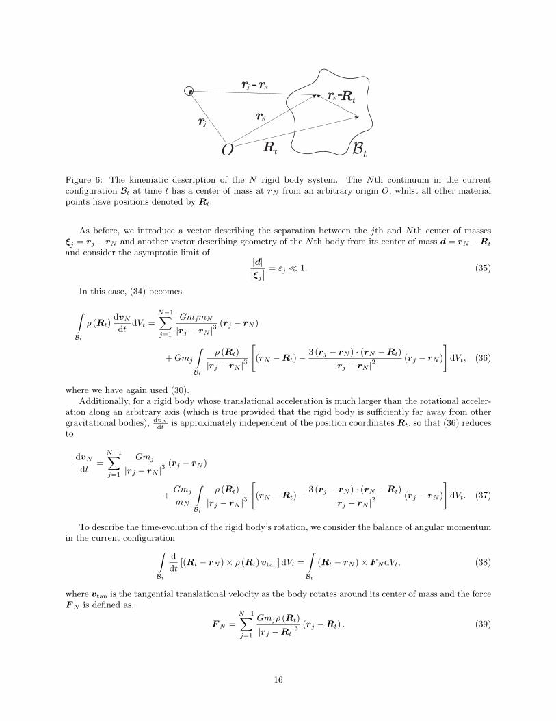
Figure 6: The kinematic description of the N rigid body system. The Nth continuum in the currentconfiguration Bt at time t has a center of mass at rN from an arbitrary origin O, whilst all other materialpoints have positions denoted by Rt.

As before, we introduce a vector describing the separation between the jth and Nth center of massesξj = rj − rN and another vector describing geometry of the Nth body from its center of mass d = rN −Rt

and consider the asymptotic limit of|d|∣∣ξj∣∣ = εj � 1. (35)

In this case, (34) becomes

∫Bt

ρ (Rt)dvNdt

dVt =

N−1∑j=1

GmjmN

|rj − rN |3(rj − rN )

+Gmj

∫Bt

ρ (Rt)

|rj − rN |3

[(rN −Rt)−

3 (rj − rN ) · (rN −Rt)

|rj − rN |2(rj − rN )

]dVt, (36)

where we have again used (30).Additionally, for a rigid body whose translational acceleration is much larger than the rotational acceler-

ation along an arbitrary axis (which is true provided that the rigid body is sufficiently far away from othergravitational bodies), dvN

dt is approximately independent of the position coordinates Rt, so that (36) reducesto

dvNdt

=

N−1∑j=1

Gmj

|rj − rN |3(rj − rN )

+Gmj

mN

∫Bt

ρ (Rt)

|rj − rN |3

[(rN −Rt)−

3 (rj − rN ) · (rN −Rt)

|rj − rN |2(rj − rN )

]dVt. (37)

To describe the time-evolution of the rigid body’s rotation, we consider the balance of angular momentumin the current configuration∫

Bt

d

dt[(Rt − rN )× ρ (Rt)vtan] dVt =

∫Bt

(Rt − rN )× FNdVt, (38)

where vtan is the tangential translational velocity as the body rotates around its center of mass and the forceFN is defined as,

FN =

N−1∑j=1

Gmjρ (Rt)

|rj −Rt|3(rj −Rt) . (39)

16

Introducing the separation vector ξj and rigid body vector d, we expand the right hand side of (38) inthe limit specified in (35) to find

−N−1∑j=1

Gmj

∫Bt

d× ρ (Rt)

(ξj + d

)∣∣ξj + d∣∣3 dVt

= −N−1∑j=1

Gmj

∫Bt

d× ρ (Rt)∣∣ξj∣∣2(ξj + εjd− 3εj

(ξj · d

)ξj +O

(ε2j))

dVt. (40)

We note that since the cross product of a constant vector with respect to integration can be interpretedas a linear transform, we have that the first term on the right hand side of (40) vanishes, because for a rigidbody of any geometry ∫

Bt

d× ρ (Rt)ξj∣∣ξj∣∣2 dVt =

∫Bt

ρ (Rt)ddVt ×ξj∣∣ξj∣∣3 = 0, (41)

given the definition of d as positions of material points in the body from the center of mass.Noting that the second term in the right hand side of (40) also vanishes as a result of the cross product

of a vector d with itself, we have a single first-order correction in εj , which simplifies (38) to∫Bt

d

dt[(Rt − rN )× ρ (Rt)vtan] dVt

∼ 3

N−1∑j=1

Gmj

∫Bt

(Rt − rN )× ρ (Rt)((rj − rN ) · (Rt − rN )) (rj − rN )

|rj − rN |5dVt,

(42)

as εj → 0.We note that the preceding equations of motion can also be derived from a gravitational potential

argument, an example of which is given in Celletti (2010) for the case of the Beletsky dumbbell.

6.2 Reduction to a one-dimensional rotating object in a plane

To obtain an explicit relation for the balance of linear and angular momentum in the quadrupole limit, wesuppose that all motion, rotational and translational, is confined to the x-y plane and we take the rigidbody to have a simple geometry; namely, a one dimensional object. The position of the ith center of mass isgiven by (xi, yi) in Cartesian coordinates. We describe the rod with an arclength coordinate in the referenceconfiguration S ∈ [−L,L] which is assumed to align with the x-axis for convenience. Under this reduction,the rigid body rotates around a single axis pointing perpendicular to the plane which we parameterize by anangular position θ with respect to the positive x-axis, so that the position vector of material points in thecurrent configuration is kinematically given by

Rt = (xN , yN ) + (S − SCOM) (cos θ, sin θ) (43)

with rN = (xN , yN ) and where SCOM is the center of mass in this one-dimensional parameterization, definedas (see Fig. 7)

SCOM =1

mN

L∫−L

ρ (S)SdS. (44)

See Fig. 7 for a diagram of this coordinate system. Note too that we have assumed that the density isparameterized in this geometry as ρ(S).

17

S=SCOM

µx

y

O

Bt

B0rN

S=LS= -L

Figure 7: The planar motion of a rotating rigid rod is described by a mapping from a reference configurationB0 to a current configuration Bt at time t. B0 is taken to align with the positive x-axis and is parameterizedby a reference arclength coordinate S ∈ [−L,L], whereby the center of mass occurs at S = SCOM using(44). The position vector rN points to the center of mass at a particular time, so that the displacement ofa material point in Rt = (xN , yN ) + (S − SCOM) (cos θ, sin θ).

With these assumptions, we simplify (33) to obtain

(d2xidt2

,d2yidt2

)=

N∑j 6=i

Gmj[(xj − xi)2 + (yj − yi)2

] 32

(xj − xi, yj − yi)

+G (cos θ, sin θ)[

(xN − xi)2 + (yN − yi)2] 3

2

L∫−L

ρ (S) (S − SCOM) dS

− 3G [(xN − xi) cos θ + (yN − yi) sin θ][(xN − xi)2 + (yN − yi)2

] 52

(xN − xi, yN − yi)L∫−L

ρ (S) (S − SCOM) dS, (45)

where we have decomposed the acceleration field and position vectors of all masses into Cartesian components.However, we note that the integral terms vanish by the definition of (44), which reduces the translational

equations of motion to the standard point mass case with higher order corrections occurring at the order ofε2i . We observe that similar reasoning leads to the same reduction for the orbital motion of the rigid bodyas (37) becomes, under the reduction of the rigid body to a 1D continuum

(d2xNdt2

,d2yNdt2

)=

N−1∑j=1

Gmj[(xj − xN )

2+ (yj − yN )

2] 3

2

(xj − xN , yj − yN )

− Gmj (cos θ, sin θ)

mN

[(xj − xN )

2+ (yj − yN )

2] 3

2

L∫−L

ρ (S) (S − SCOM) dS

+3Gmj [(xj − xN ) cos θ + (yj − yN ) sin θ]

mN

[(xj − xN )

2+ (yj − yN )

2] 5

2

(xj − xN , yj − yN )

L∫−L

ρ (S) (S − SCOM) dS, (46)

with higher order terms of ε2j .We now consider the reduction of the balance of angular momentum of the rigid body (i.e. (42)), which

18

givesL∫−L

(S − SCOM) ρ (S)d

dt

[(cos θ, sin θ, 0)×

(dxtan

dt,

dytandt

, 0

)]dS

= 3

N−1∑j=1

Gmj

L∫−L

(S − SCOM)2ρ (S) (cos θ, sin θ, 0)

×

(((xj − xN ) cos θ + (yj − yN ) sin θ) (xj − xN , yj − yN , 0)

((xj − xN )2 + (yj − yN )2)5/2

)dS,

(47)

where we note that the distance between the material point and the center of mass (S − SCOM) is independentof time for a rigid body.

Simplifying both sides, we obtain

L∫−L

(S − SCOM) ρ (S)d

dt

[dytan

dtcos θ − dxtan

dtsin θ

]dS

=3

2

N−1∑j=1

Gmj

L∫−L

(S − SCOM)2ρ (S)

2 (xj − xN ) (yj − yN ) cos 2θ((xj − xN )

2+ (yj − yN )

2)5/2

+

[(yj − yN )

2 − (xj − xN )2]

sin 2θ((xj − xN )

2+ (yj − yN )

2)5/2

dS,

(48)

where the left hand term in square brackets is the rotational velocity multiplied by the distance between thematerial point and the rod’s center of mass, (S − SCOM) dθ

dt . To show this, one could consider the relationshipbetween the angular velocity ω and the tangential translational velocity vtan

ω =(Rt − rN )× vtan|Rt − rN |2

, (49)

which, for the present case, becomes

dθ

dt=

(dytandt cos θ − dxtan

dt sin θ)

(S − SCOM). (50)

With this, the balance of angular momentum for the rotating rod reduces to

d2θ

dt2=

3G

2

N−1∑j=1

mj

(2 (xj − xN ) (yj − yN ) cos 2θ +

[(yj − yN )

2 − (xj − xN )2]

sin 2θ)

((xj − xN )

2+ (yj − yN )

2)5/2 , (51)

where the integration over S, corresponding to the moment of inertia of the rigid body, cancels from bothsides.

References

Abouelmagd, E. I., Guirao, J. & Vera, J. [2015] “Dynamics of a dumbbell satellite under the zonal harmoniceffect of an oblate body,” Communications in Nonlinear Science and Numerical Simulation 20, 1057–1069.

Arnold, V. [1964] “Instability of dynamical systems with several degrees of freedom (Instability of motionsof dynamic system with five-dimensional phase space),” Soviet Mathematics 5, 581–585.

19

Batygin, K. & Morbidelli, A. [2015] “Spin–spin coupling in the Solar System,” The Astrophysical Journal810, 110.

Beletskii, V. V. [1966] “Motion of an artificial satellite about its center of mass,” Israel Program for ScientificTranslations .

Belhaq, M., Fiedler, B. & Lakrad, F. [2000] “Homoclinic connections in strongly self-excited nonlinearoscillators: the Melnikov function and the elliptic Lindstedt–Poincare method,” Nonlinear Dynamics 23,67–86.

Boue, G. [2017] “The two rigid body interaction using angular momentum theory formulae,” Celestial Me-chanics and Dynamical Astronomy 128, 261–273.

Burov, A. A. [1984] “Non-integrability of planar oscillation equation for satellite in elliptical orbit,” VestnikMoskovskogo Universiteta. Seriya I. Matematica, Mekhanika 1, 71–73.

Camassa, R., Kovacic, G. & Tin, S.-K. [1998] “A Melnikov method for homoclinic orbits with many pulses,”Archive for Rational Mechanics and Analysis 143, 105–193.

Celletii, A. & Sidorendko, V. V. [2008] “Some properties of the dumbbell satellite attitude dynamics,”Celestial Mechanics and Dynamical Astronomy 101, 105–126.

Celletti, A. [2010] Stability and Chaos in Celestial Mechanics (Springer Science & Business Media).

Chacon, R. [2006] “Melnikov method approach to control of homoclinic/heteroclinic chaos by weak harmonicexcitations,” Philosophical Transactions of the Royal Society of London A: Mathematical, Physical andEngineering Sciences 364, 2335–2351.

Chenciner, A., Fejoz, J. & Montgomery, R. [2005] “Rotating Eights: I. the three Γi families,” Nonlinearity18, 1407.

Chenciner, A. & Montgomery, R. [2000] “A remarkable periodic solution of the three-body problem in thecase of equal masses,” Annals of Mathematics 152, 881–902.

Correia, A., Leleu, A., Rambaux, N. & Robutel, P. [2015] “Spin-orbit coupling and chaotic rotation forcircumbinary bodies-Application to the small satellites of the Pluto-Charon system,” Astronomy & As-trophysics 580, L14.

Correia, A. C. M., Boue, G., Laskar, J. & A., R. [2014] “Deformation and tidal evolution of close-in planetsand satellites using a Maxwell viscoelastic rheology,” Astronomy and Astrophysics 571.

Delisle, J.-B., Correia, A. C. M., Leleu, A. & Robutel, P. [2017] “Spin dynamics of close-in planets exhibitinglarge transit timing variations,” Astronomy and Astrophysics 605.

Dmitrasinovic, V., Hudomal, A., Shibayama, M. & Sugita, A. [2017] “Newtonian Periodic Three-BodyOrbits with Zero Angular Momentum: Linear Stability and Topological Dependence of the Period,” arXivpreprint arXiv:1705.03728 .

Dmitrasinovic, V. & Suvakov, M. [2015] “Topological dependence of Kepler’s third law for collisionlessperiodic three-body orbits with vanishing angular momentum and equal masses,” Physics Letters A 379,1939–1945.

Eddington, A. & Clark, G. [1938] “The problem of n bodies in general relativity theory,” 166, 465–475.

Fernandez-Martınez, M., Lopez, M. A. & Vera, J. [2016] “On the dynamics of planar oscillations for adumbbell satellite in J2 problem,” Nonlinear Dynamics 84, 143–151.

Frouard, J. & Compere, A. [2012] “Instability zones for satellites of asteroids: the example of the (87) Sylviasystem,” Icarus 220, 149–161.

20

Grimshaw, R. & Tian, X. [1994] “Periodic and chaotic behaviour in a reduction of the perturbed Korteweg-deVries equation,” Proceedings of the Royal Society of London A: Mathematical, Physical and EngineeringSciences (The Royal Society), pp. 1–21.

Guckenheimer, J. & Holmes, P. [2013] Nonlinear oscillations, dynamical systems, and bifurcations of vectorfields, Vol. 42 (Springer Science & Business Media).

Hogan, S. [1992] “Heteroclinic bifurcations in damped rigid block motion,” Proceedings of the Royal Societyof London A: Mathematical, Physical and Engineering Sciences (The Royal Society), pp. 155–162.

Holmes, P. & Marsden, J. [1982a] “Horseshoes in perturbations of Hamiltonian systems with two degrees offreedom,” Communications in Mathematical Physics 82, 523–544.

Holmes, P. & Marsden, J. [1982b] “Melnikov’s method and Arnold diffusion for perturbations of integrableHamiltonian systems,” Journal of Mathematical Physics 23, 669–675.

Hou, X., Scheeres, D. & Xin, X. [2017] “Mutual potential between two rigid bodies with arbitrary shapesand mass distributions,” Celestial Mechanics and Dynamical Astronomy 127, 369–395.

Hu, X. & Sun, S. [2009] “Index and Stability of Symmetric Periodic Orbits in Hamiltonian Systems withApplication to Figure-Eight Orbit,” Communications in Mathematical Physics 290, 737–77.

Jiang, Y., Zhang, Y., Baoyin, H. & Li, J. [2016] “Dynamical configurations of celestial systems comprised ofmultiple irregular bodies,” Astrophysics and Space Science 361, 306.

Jorda, L., Gaskell, R., Capanna, C., Hviid, S., Lamy, P., Durech, J., Faury, G., Groussin, O., Gutierrez, P.,Jackman, C. et al. [2016] “The global shape, density and rotation of Comet 67P/Churyumov-Gerasimenkofrom preperihelion Rosetta/OSIRIS observations,” Icarus 277, 257–278.

Lages, J., Shepelyansky, D. L. & Shevchenko, I. I. [2017] “Chaotic zones around rotating small bodies,” TheAstronomical Journal 153, 10pp.

Lara, M. [2014] “Short-axis-mode rotation of a free rigid body by perturbation series,” Celestial Mechanicsand Dynamical Astronomy 118, 221–234.

Levin, V. B. E. [1993] “Dynamics of Space Tether Systems,” Advances in the Astronautical Sciences 83.

Li, X. & Liao, S.-J. [2017] “More than six hundreds new families of Newtonian periodic planar collisionlessthree-body orbits,” arXiv preprint arXiv:1705.00527 .

Lichtenberg, A. & Lieberman, M. [2013] Regular and Chaotic Dynamics, Vol. 38 (Springer Science & BusinessMedia).

Lin, X.-B. [1990] “Using Melnikov’s method to solve Silnikov’s problems,” Proceedings of the Royal Societyof Edinburgh: Section A Mathematics 116, 295–325.

Lu, K. & Wang, Q. [2010] “Chaos in differential equations driven by a nonautonomous force,” Nonlinearity23.

Lynden-Bell, D. & Lynden-Bell, R. [1999] “Exact general solutions to extraordinary N–body problems,”Proceedings of the Royal Society of London A: Mathematical, Physical and Engineering Sciences (TheRoyal Society), pp. 475–489.

Lynden-Bell, R. [1995] “Landau free energy, Landau entropy, phase transitions and limits of metastabilityin an analytical model with a variable number of degrees of freedom,” Molecular Physics 86, 1353–1373.

Meech, K. J. & et al. [2017] “A brief visit from a red and extremely elongated interstellar asteroid,” Nature552, 378–381.

Meiss, J. [1992] “Symplectic maps, variational principles, and transport,” Reviews of Modern Physics 64,795.

21

Melnikov, A. & Shevchenko, I. [2010] “The rotation states predominant among the planetary satellites,”Icarus 209, 786–794.

Mel’nikov, V. [1963] “On the stability of a center for time-periodic perturbations,” Trudy moskovskogomatematicheskogo obshchestva 12, 3–52.

Moeckel, R. [1990] “On central configurations,” Mathematische Zeitschrift 205, 499–517.

Moeckel, R. [2017] “Minimal energy configurations of gravitationally interacting rigid bodies,” CelestialMechanics and Dynamical Astronomy 128, 3–18.

Moore, C. [1993] “Braids in classical dynamics,” Physical Review Letters 70, 3675.

Musielak, Z. & Quarles, B. [2014] “The three-body problem,” Reports on Progress in Physics 77, 065901.

Mysen, E. [2009] “On the predictability of unstable satellite motion around elongated celestial bodies,”Astronomy & Astrophysics 506, 989–992.

Mysen, E., Olsen, Ø. & Aksnes, K. [2006] “Chaotic gravitational zones around a regularly shaped complexrotating body,” Planetary and Space Science 54, 750–760.

Nauenberg, M. [2001] “Periodic orbits for three particles with finite angular momentum,” Physics Letters A292, 93–99.

Nauenberg, M. [2007] “Continuity and stability of families of figure eight orbits with finite angular momen-tum,” Celestial Mechanics and Dynamical Astronomy 97, 1–15.

Papakostas, S. & Tsitouras, C. [1999] “High Phase-Lag-Order Runge–Kutta and Nystrom Pairs,” SIAMJournal on Scientific Computing 21, 747–763.

Quillen, A. C., Nichols-Fleming, F., Chen, Y.-Y. & Noyelles, B. [2017] “Obliquity evolution of the minorsatellites of Pluto and Charon,” Icarus 293, 94–113.

Roberts, G. E. [2007] “Linear stability analysis of the figure-eight orbit in the three-body problem,” ErgodicTheory and Dynamical Systems 27, 1947–1963.

Showalter, M. & Hamilton, D. [2015] “Resonant interactions and chaotic rotation of Pluto’s small moons,”Nature 522, 45–49.

Spyrou, K. & Thompson, J. [2000] “The nonlinear dynamics of ship motions: a field overview and some recentdevelopments,” Philosophical Transactions of the Royal Society of London A: Mathematical, Physical andEngineering Sciences 358, 1735–1760.

Suvakov, M. & Dmitrasinovic, V. [2013] “Three classes of Newtonian three-body planar periodic orbits,”Physical review letters 110, 114301.

Tarnopolski, M. [2017a] “Influence of a second satellite on the rotational dynamics of an oblate moon,”Celestial Mechanics and Dynamical Astronomy 127, 121–138.

Tarnopolski, M. [2017b] “Rotation of an oblate satellite: Chaos control,” Astronomy & Astrophysics 606,A43.

Weaver, H., Buie, M., Buratti, B., Grundy, W., Lauer, T., Olkin, C., Parker, A., Porter, S., Showalter,M., Spencer, J. et al. [2016] “The small satellites of Pluto as observed by New Horizons,” Science 351,aae0030.

Wiggins, S. [1987] “Chaos in the quasiperiodically forced duffing oscillator,” Physics Letters A 124, 138–142.

Wiggins, S. [2003] Introduction to applied nonlinear dynamical systems and chaos, Vol. 2 (Springer Science& Business Media).

22

Wisdom, J., Peale, S. J. & Mignard, F. [1984] “The chaotic rotation of Hyperion,” Icarus 58, 137–152.

Xia, Z. [1992] “Melnikov method and transversal homoclinic points in the restricted three-body problem,”Journal of differential equations 96, 170–184.

Yagasaki, K. [1994] “Homoclinic motions and chaos in the quasiperiodically forced van der Pol-Duffingoscillator with single well potential,” Proceedings of the Royal Society of London A: Mathematical, Physicaland Engineering Sciences (The Royal Society), pp. 597–617.

Yagasaki, K. [1999] “The method of Melnikov for perturbations of multi-degree-of-freedom Hamiltoniansystems,” Nonlinearity 12, 799.

Zhang, W., Yao, M. & Zhang, J. [2009] “Using the extended Melnikov method to study the multi-pulseglobal bifurcations and chaos of a cantilever beam,” Journal of Sound and Vibration 319, 541–569.

Zhang, W., Zhang, J. & Yao, M. [2010] “The extended Melnikov method for non-autonomous nonlineardynamical systems and application to multi-pulse chaotic dynamics of a buckled thin plate,” NonlinearAnalysis: Real World Applications 11, 1442–1457.

Zotos, E. E. [2015] “Orbit classification in the planar circular Pluto-Charon system,” Astrophysics and SpaceScience 360, 7.

23