Wireless Sensor Networks for Underwater

Localization: A Survey

TECHNICAL REPORT: CES-521

ISSN 1744-8050

Sen Wang and Huosheng Hu

School of Computer Science and Electronic Engineering

University of Essex, Colchester CO4 3SQ, United Kingdom

Email: swangi@essex.ac.uk; hhu@essex.ac.uk

May 30, 2012

Abstract

Autonomous Underwater Vehicles (AUVs) have widely deployed in marine investigation and ocean

exploration in recent years. As the fundamental information, their position information is not only for

data validity but also for many real-world applications. Therefore, it is critical for the AUV to have

the underwater localization capability. This report is mainly devoted to outline the recent advance-

ment of Wireless Sensor Networks (WSN) based underwater localization. Several classic architectures

designed for Underwater Acoustic Sensor Network (UASN) are briefly introduced. Acoustic propa-

gation and channel models are described and several ranging techniques are then explained. Many

state-of-the-art underwater localization algorithms are introduced, followed by the outline of some

existing underwater localization systems.

Contents

1 Introduction 1

2 UASN Architectures 3

2.1 Two-Dimensional and Three-Dimensional Systems . . . . . . . . . . . . . . . . . . . . . . 3

2.2 Long-Term NTC and Short-Term TC Systems . . . . . . . . . . . . . . . . . . . . . . . . 3

2.3 AUVs-based System . . . . . . . . . . . . . . . . . . . . . . . . . . . . . . . . . . . . . . . 4

2.4 Summary . . . . . . . . . . . . . . . . . . . . . . . . . . . . . . . . . . . . . . . . . . . . . 5

3 Underwater Acoustic Propagation and Ranging 6

3.1 Underwater Acoustic Propagation and Channel Models . . . . . . . . . . . . . . . . . . . 6

3.1.1 Disturbance and Noise . . . . . . . . . . . . . . . . . . . . . . . . . . . . . . . . . . 6

3.1.2 Mathematical Model . . . . . . . . . . . . . . . . . . . . . . . . . . . . . . . . . . . 7

3.2 Solutions to Ranging . . . . . . . . . . . . . . . . . . . . . . . . . . . . . . . . . . . . . . . 8

3.2.1 Time of Arrival . . . . . . . . . . . . . . . . . . . . . . . . . . . . . . . . . . . . . . 9

3.2.2 Time Difference of Arrival . . . . . . . . . . . . . . . . . . . . . . . . . . . . . . . . 11

3.2.3 Received Signal Strength Indicator . . . . . . . . . . . . . . . . . . . . . . . . . . . 11

3.3 Several Established Localization Methods . . . . . . . . . . . . . . . . . . . . . . . . . . . 11

3.4 Summary . . . . . . . . . . . . . . . . . . . . . . . . . . . . . . . . . . . . . . . . . . . . . 13

4 Localization Algorithm 14

4.1 Localization for Stationary Networks . . . . . . . . . . . . . . . . . . . . . . . . . . . . . . 15

4.1.1 Underwater Positioning System . . . . . . . . . . . . . . . . . . . . . . . . . . . . . 15

4.1.2 Hyperbola-based Approach . . . . . . . . . . . . . . . . . . . . . . . . . . . . . . . 15

4.1.3 Anchor Free Localization . . . . . . . . . . . . . . . . . . . . . . . . . . . . . . . . 16

4.1.4 Simultaneous Localization and Synchronization . . . . . . . . . . . . . . . . . . . . 16

4.1.5 Large-Scale Hierarchical Localization . . . . . . . . . . . . . . . . . . . . . . . . . . 17

4.1.6 Underwater Sensor Positioning . . . . . . . . . . . . . . . . . . . . . . . . . . . . . 18

4.1.7 Localization Scheme for Large Scale Underwater Networks . . . . . . . . . . . . . . 18

4.1.8 Three-Dimensional Underwater Localization . . . . . . . . . . . . . . . . . . . . . . 18

4.1.9 Comparison . . . . . . . . . . . . . . . . . . . . . . . . . . . . . . . . . . . . . . . . 19

4.2 Localization for Mobile Networks . . . . . . . . . . . . . . . . . . . . . . . . . . . . . . . . 20

4.2.1 Monte Carlo Localization . . . . . . . . . . . . . . . . . . . . . . . . . . . . . . . . 20

4.2.2 Passive Mobile Robot Localization . . . . . . . . . . . . . . . . . . . . . . . . . . . 22

4.2.3 Moving-baseline Localization . . . . . . . . . . . . . . . . . . . . . . . . . . . . . . 22

4.2.4 Scalable Localization with Mobility Prediction . . . . . . . . . . . . . . . . . . . . 22

4.2.5 AUV-aided Localization . . . . . . . . . . . . . . . . . . . . . . . . . . . . . . . . . 23

4.2.6 Dive and Rise Localization . . . . . . . . . . . . . . . . . . . . . . . . . . . . . . . 23

4.2.7 Simultaneous Localization and Environmental Mapping . . . . . . . . . . . . . . . 24

4.3 Localization for Mobile Swarm . . . . . . . . . . . . . . . . . . . . . . . . . . . . . . . . . 25

4.3.1 Motion-Aware Self Localization . . . . . . . . . . . . . . . . . . . . . . . . . . . . . 25

4.3.2 Collaborative Localization . . . . . . . . . . . . . . . . . . . . . . . . . . . . . . . . 25

4.3.3 Monte Carlo Localization . . . . . . . . . . . . . . . . . . . . . . . . . . . . . . . . 26

4.4 Summary . . . . . . . . . . . . . . . . . . . . . . . . . . . . . . . . . . . . . . . . . . . . . 26

5 Existing Underwater Sensor Network Systems 27

5.1 Traditional Underwater Positioning Systems . . . . . . . . . . . . . . . . . . . . . . . . . . 27

5.2 Localization Systems for Underwater Robots . . . . . . . . . . . . . . . . . . . . . . . . . 28

5.2.1 Systems Using the Stationary or Semi-stationary Beacons . . . . . . . . . . . . . . 28

I

5.2.2 Systems Without Static Beacon . . . . . . . . . . . . . . . . . . . . . . . . . . . . . 29

5.2.3 Localization System for Robotic Fish . . . . . . . . . . . . . . . . . . . . . . . . . . 29

5.3 Summary . . . . . . . . . . . . . . . . . . . . . . . . . . . . . . . . . . . . . . . . . . . . . 30

6 Conclusions 31

II

1 Introduction

Oceans cover about 71% of the earth’s surface, but most of them have not been explored. Recently,

the exploration on oceans is significantly increasing since they are rich in valuable resources. Moreover,

sea is one of the most important ecological environment for human being. Therefore, many studies are

undertaken to protect the ocean from being influenced [1].

Most of these marine application and investigation rely on the AUVs to accomplish the task now. The

location of the AUVs is very important because the application cannot know where the data is sampled

unless the location is tagged. In other words, the information is useless without the corresponding

location. The AUV also requires its current position to make the decision for the control and navigation.

Therefore, the localization is regarded as a basic capability of AUV if it is going to track a target [2],

explore the resources [3], monitor the underwater environment, etc. Apart from the significance for

AUV, the localization can also improve the performance of the system, such as the location-based routing

protocol [4].

According to the used hardware, the means of underwater localization can be categorized into three

types [5]:

� Inertial navigation systems. The compass, Inertial Measurement Unit (IMU), Doppler Velocity Log

(DVS), etc. can be employed to estimate the position. The position calculated by twice integration

of the sensed acceleration is normally better than dead-reckoning in terms of localization accuracy.

However, the additional acceleration produced by the ocean current is difficult to be distinguished

from the real one. Another drawback is the unbounded position error. Therefore, some new

techniques are proposed to update the position using satellite navigation system [6]. Although the

accuracy is improved, the AUV possibly collides with the surface vessels when it emerges from water

to refine the location, especially near the coast and the port.

� Geophysical navigation. This method estimates the location by matching the measured geophysical

parameter with that in the pre-built environment map. The parameters are usually the physical

features of the environment, e.g. magnetic field. Now it is widely used in the submarines to achieve

the accurate navigation [7]. However, it is unsuitable for the AUV because the environment should

be mapped in advance and the map construction, the data searching, etc. are time- and energy-

consuming.

� Communication navigation. Because the distance between the beacon and the AUV can be esti-

mated by communication, the location can be derived by the localization algorithms without extra

consumption especially for a swarm of AUVs. However, the acoustic signal is the unique suitable

technique to make the underwater communication viable since the radio frequency (RF) and optical

signal only propagate a very short distance in water due to the absorption, attenuation and scatter-

ing. This is also why the WSN is usually replaced by the UASN when the underwater environment

is discussed.

As a new and promising approach developing in recent years, the UASN has many inherent advantages

[3, 8] and attracts more attention. On the other hand, it operates under the following constraints and

challenges, which are produced by the extreme features of water environment and the restrictions of the

acoustic signal:

� Serious disturbance and noise. The underwater acoustic communication and channel are consid-

erably influenced by the dynamic water environment (e.g. temperature, density and depth) and

various disturbances (e.g. path loss and multi-path). All these cause the propagation path to be

complicated with temporal and spatial variation. Meanwhile, the channel is subjected to man made

and ambient noise, which produce uncertain perturbations to the system constantly. The detail

will be discussed in Section 3.

� Poor link quality and high bit error rates. Because the communication link suffers from various

disturbance and noise, the underwater acoustic channel has low link quality and the connectivity is

1

not reliable. Therefore, the probability of error rate is high, especially when there are some sudden

noises.

� Long latency. The physical transformation of communication from RF to acoustics changes the

signal propagation speed from light to sound, which indicates the propagation delay is five orders of

magnitude longer under the water than in the air. Therefore, time synchronization is indispensable.

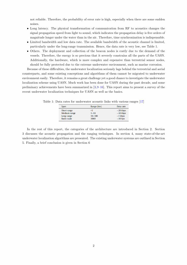
� Limited bandwidth and low data rate. The available bandwidth of the acoustic channel is limited,

particularly under the long-range transmission. Hence, the data rate is very low, see Table 1.

� Others. The deployment and collection of the beacon nodes is costly due to the demand of the

vessels. Therefore, the energy is so precious that it severely constrains all the parts of the UASN.

Additionally, the hardware, which is more complex and expensive than terrestrial sensor nodes,

should be fully protected due to the extreme underwater environment, such as marine corrosion.

Because of these difficulties, the underwater localization seriously lags behind the terrestrial and aerial

counterparts, and some existing conceptions and algorithms of them cannot be migrated to underwater

environment easily. Therefore, it remains a great challenge yet a good chance to investigate the underwater

localization scheme using UASN. Much work has been done for UASN during the past decade, and some

preliminary achievements have been summarized in [3,9–16]. This report aims to present a survey of the

recent underwater localization techniques for UASN as well as the basics.

Table 1: Data rates for underwater acoustic links with various ranges [17]

In the rest of this report, the categories of the architecture are introduced in Section 2. Section

3 discusses the acoustic propagation and the ranging techniques. In section 4, many state-of-the-art

underwater localization algorithms are presented. The existing underwater systems are outlined in Section

5. Finally, a brief conclusion is given in Section 6

2

2 UASN Architectures

Nowadays, most of the UASN based localization algorithm and system can be generally divided into

range-free and range-based localizations depending on how the unknown location is calculated. The

range-free localization, which is simple yet needs large-scale sensor nodes, entirely relies on the proximity

and connectivity between the the beacon and the unknown node, e.g. MAP-M and MAP-M&N [18].

In general, there are two types of range-free localization techniques that have been proposed for sensor

networks: local techniques and hop-based techniques [19], both of which require a very high density of

beacons and consume excessive energy during the frequent data broadcast and transfer. Because the

sensor cost and the energy value in the UASN system are much higher than terrestrial one, the range-free

based localization is unsuitable for the underwater localization.

For the range-based scheme, the location of unknown node can be determined by the localization

algorithm once the distance or angle between the unknown node and the beacon is measured. This

approach outperforms the range-free localization in terms of the beacon number and localization accuracy.

Note that the AUV can be considered as the unknown node in UASN. In this report, our attention focuses

on the range-based localization.

For the different underwater architectures, the beacons can be anchored in the sea floor or attached

to the floating buoy (in such case the buoy can freely drift along with the sea current or be tethered to

a rude position), which dramatically influences the localization algorithm, implementation as well as the

system performance. Therefore, some typical architectures are outlined in this section.

2.1 Two-Dimensional and Three-Dimensional Systems

The UASN systems can be classified as two-dimension or three-dimension according to the spatial coverage

[20].

A reference two-dimensional architecture [3] is shown in Fig. 1. All the nodes are anchored to the

ocean floor which is assumed to be a plain. By the horizontal transceiver, uw-sink can collect the data

from the sensor nodes. Then, it relays the information to a surface station by the vertical transceiver.

The surface station has RF signal to efficiently communicate with the onshore and surface sinks, where

the sensed data is processed. For this scheme the uw-sink and the sensor node can be the unknown node

and beacon respectively.

Figure 1: A two-dimensional UASN [3]

However, it is necessary to investigate the three-dimensional localization since it is much closer to our

3

real world and many tasks cannot be accomplished in two-dimension, such as the research on the species

diversity with respect to different ocean depths. In [21], a three-dimensional architecture is discussed, see

Fig. 2. Each uw-sensor node is attached to a buoy by a cable, which can also transmit data between each

other. The lengths of the cables are different for the requirement of the three-dimensional localization.

When the sensed data is received by the buoy, it is transmitted to the central station by RF signal.

However, the buoy randomly drifts along the sea current, which may obstruct or collide with the vessels.

The scheme whose sensor nodes are anchored to the bottom can overcome this [3]. As shown in Fig. 3,

the sensor node floating under the water is tethered with a wire, which is fixed to the ocean floor and

has the adjustable length. The AUV can shuttle in the surveillance region covered with these beacons.

The communication principle is the same as the one described in Fig. 1 except that the surface station

can receive the data from the sensor nodes directly.

Figure 2: A three-dimensional UASN where sensors float with buoy [21]

Figure 3: A three-dimensional UASN where sensors are deployed on the sea floor [4]

2.2 Long-Term NTC and Short-Term TC Systems

Cui et al. [22] present the long-term non-time-critical (NTC) and the short-term time-critical (TC) archi-

tectures for mobile UASN, see Fig. 4. Because the first one aims at long-term underwater applications,

e.g. pollution detection and monitoring, the hardware, communication mechanism, localization algorithm

etc. should be energy saving. In contract, the short-term time-critical system regards the real-time data

4

(a) Long-term non-time-critical system (b) Short-term time-critical system

Figure 4: Architecture of mobile UASNs [22]

transfer as the most important criterion. For example, the detection of an enemy’s submarine should be

transferred to the headquarters as soon as possible. The nodes in these two architectures both relay data

via multi-hop acoustic routes.

2.3 AUVs-based System

Because the AUVs can shuttle in the ocean, an architecture where the network connectivity relies on the

AUV is proposed [10]. The AUV visits the sparsely deployed nodes periodically to collect the sensed and

stored data with the aid of an optical location system. When the distance between the AUV and the

destination node is short enough, the data is transmitted by acoustic communication. Although saving

the energy of the node and improving the data transfer rate simultaneously are the advantages of this

method, the optical location system is influenced by the scattering, beam divergence and ambient light,

and it takes too much time for an AUV to collect all the data in a large region. Moreover, the system

only can monitor the area where the sensors deployed since the AUV does not perceive the environment.

2.4 Summary

The existing architectures have their own characters and application areas. The architecture which highly

determines the further choice of sensor, communication method, localization algorithm, implementation,

etc. should be designed first according to the application environment and performance requirement.

5

3 Underwater Acoustic Propagation and Ranging

Because the RF signal and optical wave are unsuitable for the underwater propagation, most of the

underwater systems employ the acoustic signal as the communication technique. On the one hand,

the complex and uncertain characteristics of the underwater environment result in many big challenges

in acoustic propagation, which is essentially sensitive to the disturbances. On the other hand, the

performance, such as the accuracy, has to satisfy the various requirements of the application scenario.

Therefore, the underwater acoustic channel should be studied to comprehend the characters of the acoustic

signal.

The existing WSN localization generally contains two stages: measuring the geographic information

from the network and computing the locations with this measured data. In this section, the basics of

acoustic propagation and the solutions of ranging are briefly introduced, which is considered as the first

step.

3.1 Underwater Acoustic Propagation and Channel Models

Underwater acoustic communication is seriously affected by many factors, which make the underwater

propagation channel enormously complex. They can be temperature, density, path loss, noise, multi-

path propagation, Doppler effect, propagation delay etc. In order to design and improve the localization

algorithm with clear orientation, these disturbances and noises as the chief influences on the performance

should be studied.

3.1.1 Disturbance and Noise

Underwater acoustic channel suffers from various disturbances and noises, which severely reduce the

ranging accuracy. They are mainly [3]:

� Disturbance. (1) Path loss: The acoustic signal propagates under the water, working off some

sound energy. One of the two reasons is attenuation. The absorption as well as the scattering

and reverberation consume a great deal of energy during the propagation. The other is geometric

spreading, which can be spherical or cylindrical according to the different depths. The cylindrical

spreading is suitable for the the shallow waters while the spherical one is for the deep sea. (2) Multi-

path effect: The reflection, especially provoked by the ocean surface and floor, is the main cause

of the multi-path propagation. Because the temperature and density in the varying depths of the

ocean are different, reflection also exists in the liquid interface [8]. The weighted Gerchberg-Saxton

algorithm (WGSA) as a solution can identify the direct path and mitigate the effects of multiple

range measurements [23]. (3) Doppler effect: The Doppler effect produced by the relative movement

of the transducer and the transponder is the phenomenon that the observer receives a wave with

the changing frequency. The Doppler effect of UASNs is particularly serious due to the slow sound

velocity.

� Time and Space Variability of Water Medium. Owing to the varying physical properties of the

ocean and the constant perturbations created by the environment, the underwater acoustic channel

is endowed with temporal and spatial variability, which severely affect the time synchronization and

localization accuracy.

� Noise. There are two types of noise - man made and ambient noises. The man made noise is usually

caused by the marine machinery, such as the offshore drilling platform and the vessel, while the

ambient noise is generated by the tides, sea current, storms, wind and rain as well as the biological

activities like fishes swimming etc. Some of the ambient noise is so strong that the UASN may be

destroyed.

6

3.1.2 Mathematical Model

As described in Fig. 5, the modeling plays a key role in the experiment and analysis. In order to

analyze the system and process the data, the mathematical models of the acoustic propagation, noise etc.

should be developed. Because the discipline of underwater acoustics has been studied for many years,

there are some available theories and models. However, the models have their own inherent advantages,

disadvantages and restrictions.

Figure 5: Schematic relationship between experiment and modeling [24]

Speed The underwater sound speed model has been developed over the years for the exact mathe-

matical relationship between it and the ocean properties. Many models have been produced after a

tremendous amount of scientific work, and some of them are summarized in Table 2. It can be seen

that the temperature, salinity and pressure, which is related to the depth, are usually considered as the

main factors that affect the sound speed even though the numbers of the terms are different. The model

should be chosen according to the ranges of its properties and the accuracy. The expression of the formula

Mackenzie (1981) of the sound speed at a particular depth is

c = 1448.96 + 4.591T − 5.304× 10−2T 2 + 2.374× 10−4T 3 + 1.340(S − 35)

+1.630× 10−2D + 1.675× 10−7D2 − 1.025× 10−2T (S − 35)− 7.139× 10−13TD3(1)

where c is the speed of sound in m/s, T is the water temperature in Celsius, S is the salinity in practical

salinity units and D is the depth in meter. For the issue of determining these environment parameters,

they can be easily accessed from the existing databases, such as the Bedford Institute of Oceanography

(BIO), National Physical Laboratory (NPL) and the National Oceanic and Atmospheric Administration

(NOAA), which are constructed using the actual data collected from the ocean.

Acoustic Propagation Model Most of the terrestrial propagation models assume that they only

relate to the transmission distance, but the signal frequency also affects the underwater acoustic prop-

agation. The acoustic propagation models can be divided into five categories according to the applied

theoretical method: ray theory model, normal mode model, multi-path expansion model, fast field model

and parobolic equation model. They are derived from the wave equation, Harmonic solution or Helmholtz

equation, and their relationships have been summarized in Fig. 6. Each model can be further divided

into many specific models, see Table 3. It can be seen that there are more than 100 established models

like BELLHOP [25]. Therefore, choosing the appropriate model is quite difficult. Table 4 provides the

applicable domains of these five general models, which can be used to narrow down the choices. The char-

acters of each specific model should be referred and it can be tested in reality to compare the performance

when selecting the candidate models.

7

Table 2: Summary of sound speed algorithms and parameter ranges [24]

Figure 6: Summary of relationships among propagation modeling [24]

Noise Model Mathematical models of noise in the ocean can be classified into ambient-noise models

and beam-noise statistics models. The noise sources of ambient model are surface weather, biologic

activities, shipping and oil drilling. The beam-noise models, which can be further divided into analytic

and simulation approaches, are good at the application which has low-frequency shipping noise. Some

typical noise models are summarized in Table 5.

3.2 Solutions to Ranging

With the aid of the acoustic propagation models, the distance between the devices can be estimated by

ranging method. The time of arrival (TOA), time difference of arrival (TDOA), received signal strength

indicator (RSSI) and angle of arrival (AOA) are the four typical ranging techniques of the WSN system.

The requirement and constrain on ranging hardware, measurement accuracy, energy consumption etc.

should be comprehensively considered when choosing the ranging approach. The TOA, TDOA and AOA

are more appropriate for the application which requires a high localization accuracy, such as resource

exploration or environment monitoring, while the RSSI is better for saving energy.

8

Table 3: Summary of underwater acoustic propagation models [24]

3.2.1 Time of Arrival

Assuming the velocity of sound has already been known, Time of Arrival (TOA) uses the signal traveling

time from the transmitter to receiver to measure the distance. According to the propagation theory, the

distance in Fig. 7 equals to

Dist = V · T = V · (T2 − T1) (2)

where V is the spreading speed, and T is the traveling time which is the time difference between the

transmitting time T1 and the arrival time T2. Sound is the commonly used signal because the velocity of

radio frequency is so fast that the time is too short to be counted. Although the range accuracy of this

method is relatively high, the time synchronization which is difficult for a large scale WSN is required.

Moreover, the slow speed of sound aggravates the Doppler effect in the UASN. By contrast, the symmetric

double sided two-way ranging approach [27,28] can avoid the time synchronization and the uncertainties,

such as the misalignment between the actual signal emission and the time delay of recognition of signal

arrival. As described in Fig. 8, the B transmits a signal at TB1. The A receives this signal and sends

back an acknowledgment signal at TA1 and TA2 respectively. The B receives the returned package at

9

Table 4: Domains of applicability of underwater acoustic propagation models [24] [26]

Table 5: Summary of underwater acoustic noise models [24]

TB2. TAi and TBi are belong to the local clock of A and B respectively. Then, TA1 = TB1 + ∆ + TProp

and TB2 = TA2 − ∆ + TProp, where ∆ is the time difference between the local clocks of the A and B,

TProp is the propagation time of one single route. Hence, the following equation can be used to measure

the distance:

Dist = V · TProp = V · (TA1 + TB2 − TB1 − TA2)

2, (3)

This method can not only has the accuracy as good as one-way TOA’s, but also does not need the time

synchronization. However, the more energy consumption trades off with these advantages.

Figure 7: TOA

Figure 8: TOA without time synchronization

10

3.2.2 Time Difference of Arrival

Time Difference of Arrival (TDOA) measures the distance by two different types of signals. As shown

in Fig. 9, the transducer A can transmit a RF signal (green line) and an ultrasonic sound (yellow line)

simultaneously. The RF signal is usually considered to be received by the transponder B immediately

since it propagates as fast as light. However, it takes a while for the ultrasonic sound to arrive at

B. Consequently, the transponder B receives the two signals at different times. When both of them

transmitted by A are received, the distance can be calculated by

Dist = V2 · TB = V2 · (TB2 − TB1), (4)

where Dist is the estimated distance, V2 is the sound propagation velocity, and TB2 and TB1 are the

arrival times of the RF and sound by the clock of B respectively. Although TDOA has the good ranging

accuracy as TOA without time synchronization, it needs more hardware and energy to generate, detect

and process the different signals.

Figure 9: Time Difference of Arrival

3.2.3 Received Signal Strength Indicator

Received Signal Strength Indicator (RSSI) estimates the distance by measuring the signal strength, which

has the mathematical relationship with distance since the signal is attenuated during the propagation.

Theoretically, the weaker the received signal is, the longer the distance is. The signal strength can be

measured during the communication without extra hardware or energy. Therefore, RSSI is an energy-

saving and low-cost method. However, it is so sensitive to the disturbances that the distance estimation

is very imprecise, especially in the underwater environment.

3.3 Several Established Localization Methods

Before discussing the state-of-the-art underwater localization schemes, some basic methods which are the

fundamental of the various localization algorithms need to be introduced. Moreover, several established

localization algorithms, which are widely used in the terrestrial and arial localization, are described here.

Trilateration The trilateration determines the location using the geometrical constraints of circles or

spheres. The location is the intersection point of the three circles or four spheres in the two-dimension or

three-dimension respectively, see Fig. 10 and Fig. 11. However, the estimated distances must have some

errors in reality, changing the intersection from a point to an overlapped area or solid. Consequently,

some additional processes are required to get the location.

11

Figure 10: Two-dimensional trilateration Figure 11: Three-dimensional trilateration

Least Squares Method By contrast, least squares method (LSM) is better than trilateration [29] since

it is difficult for the trilateration to perform the accurate localization when suffering from the various

noises. As shown in Fig. 12, there is an unknown node which measures the distances to the n beacons.

The Bi is the ith beacon with the corresponding coordinate value (xi, yi) and estimated distance di.

Hence, the LSM problem can be formulated as

√(x− x1)2 + (y − y1)2 = d1√(x− x2)2 + (y − y2)2 = d2

...√(x− xn)2 + (y − yn)2 = dn

(5)

where (x, y) is the location of the unknown node. The equations can be rewritten as

AX = b (6)

where X = [x y]T and

A =

2(x1−xn) 2(y1−yn)

......

2(xn−1−xn) 2(yn−1−yn)

b =

x1

2−xn2+y1

2−yn2+dn

2−d12

...

xn−12−xn

2+yn−12−yn

2+dn2−d1

2

(7)

The optimal solution of (6) is the X that reaches the minimum of ‖AX − b‖2, which is

‖AX − b‖22 = (AX − b)T (AX − b) = XTATAX − 2XTAT b+ bT b. (8)

Let the gradient of (8)

2ATAX − 2AT b = 0 (9)

equal zero, then

X̂ = (ATA)−1AT b. (10)

X̂ is the optimal location of the unknown node. The three-dimensional case can be derived by referring

to the above analysis.

Figure 12: Least squares method

12

Optimization Method WSN localization can be transformed into the optimization problem. Its key

idea is to minimize the differences between the measured distances and the corresponding Euclidean

distances. Maximum likelihood estimation is a typical optimization method. A variety of numerical

approaches can solve the optimization method and search the global or local optimal result, for example,

multi-resolution search algorithm [30], particle swarm optimization technique [31], conjugate-gradient [32]

and the Newton-Raphson method [33].

Multidimensional Scaling Map Multidimensional scaling (MDS) algorithm, which is recognized as

an algorithm with good performance [34], introduces the statistical techniques to perform the accurate

WSN localization [35]. Both a relative map and an absolute map are constructed during the computation.

First, the shortest path between each pair of nodes is created. Then, with only three or four beacons, the

relative map created by MDS is transformed to the absolute map, which is the final localization result.

Its main problem is the high energy consumption and the centralized property. The result is also highly

influenced by the irregularly shaped network, where the shortest path distance does not correspond well

to the Euclidean distance. A distributed MDS-MAP, namely MDS-MAP(P), is proposed to realize the

distributed localization with low computation [36]. It builds many local maps at each node and then

merge them together to form a global map. MDS-MAP(P) can tackle the non-convex deployment problem

with high accuracy and low computational complexity.

Semi-definite Programming Semi-definite programming (SDP) method represents the WSN local-

ization as a constrained programming problem [37]. It converts the geometric constraints of sensors to

a group of linear matrix inequalities. By solving this semi-definite programming problem, the satisfied

localization result can be obtained. However, the localization error may be high because of the max-rank

property of the SDP solution. In [38], both the regularization term and optimization methods are de-

signed to reduce the rank of the SDP. Unfortunately, there is no efficient way to determine an important

parameter used in the regularization term.

Iterative Localization Iterative localization can be employed to overcome drawback of limited net-

work coverage and provide more anchors [39]. It qualifies the sensors that have already been localized

as the anchors to assist the unlocalized nodes. Although this mechanism extremely improves the local-

ization rate, the localized sensors certainly have some errors in the position estimation, which inevitably

propagate and are further accumulated as the localization procedure. Therefore, the control of the error

propagation is critical for the localization schemes introduced the iterative localization.

3.4 Summary

In this section, the communication channel, ranging method and some localization algorithms which

are mainly used for the terrestrial localization are introduced. The important features of the ranging

techniques are summarized in the Table 6. When designing the UASN localization, these factors should

be considered before the ranging technique is determined.

Table 6: Summary of ranging techniquesName Hardware (Sort) Accuracy Time Synchronization Energy Consumption

One-Way TOA One High Yes MediumTwo-Way TOA One High No High

TDOA Two High No HighRSSI One Low No Low

13

4 Localization Algorithm

Localization algorithm usually uses the geographic information of their neighbor nodes to estimate the

location. Because its design closely depends on various factors, including system deployment, available

resources, accuracy requirements, etc., each algorithm almost aims for the specific application with its

own merits and drawbacks, which implies there is no algorithm which is applicable across the spectrum so

far. Therefore, the application properties and requirements should be sufficiently investigated before its

design. However, the primary goal of all localization algorithms is to make the localized position accurate

by mitigating the effects of noises, and reasonably balance the performance and the various constraints.

Even though the underwater and terrestrial localizations have some in common, they are extremely

different due to the challenges, such as serious disturbances, poor link quality, high bit error rate, long

latency, limited bandwidth, low data rate, etc. In this section, many established underwater localization

algorithms are introduced to provide a great number of references for the UASN design.

The localization schemes are divided into three categories in this report according to the sensor

mobility: stationary network, mobile network and mobile swarm.

� Stationary network. In the stationary network, all the sensors are static including the unknown

nodes. This is an ideal scenario in the underwater environment because the underwater sensors

are inevitably being pushed due to the ocean current, shipping activities, etc. However, it is the

fundamental for the other two networks.

� Mobile network. Generally, mobile network can be further divided into three types [19]: unknown

nodes are static, while beacons are moving; unknown nodes are moving, while beacons are static;

both unknown nodes and beacons are moving. In this report, the mobile network mostly represents

the second one, and the third one is called mobile swarm. As shown in Fig. 13, the mobile

network constitutes the tethered beacons, which only can be deployed roughly owing to the ocean

environment, and moving sensors (AUVs and nodes). Because the beacons always sway around

the fixed positions without updating, the known beacon locations are inaccurate. Meanwhile, the

mobile feature of the unknown nodes brings greater challenges to accurately localize them.

� Mobile swarm. It is a more complicated scheme for WSN localization, see Fig. 14. Because of the

ocean environment (currents, wind, etc.) or the actuators equipped for motion, the beacons and

sensors both have the motion capabilities. The beacons can also be self-localized (e.g., via GPS).

The movement feature overcomes the disadvantages that the WSN based localization only can be

used for the limited area with pre-deployed beacons and the network cannot service the pelagic

applications. Because the unknown nodes and AUVs cooperate with each other by communication,

the range and locations can be determined during this process without extra consumption.

Figure 13: Mobile network Figure 14: Mobile swarm

14

4.1 Localization for Stationary Networks

In general, schemes that belong to this category have static beacons whose locations can be determined

through GPS or pre-deployment depending on whether they are deployed on the surface buoys or the sea

floor. Because the unknown nodes are also static, the localization is completed once they are all located.

This kind of network is being widely investigated and some solutions are proposed in resent years.

4.1.1 Underwater Positioning System

Underwater positioning system (UPS) is a silent positioning scheme which comprises two steps [40]. The

time differences of the signal arrival are computed by frequent communications between every beacon and

sensors at first, and then they are transformed into the corresponding ranges. The second phase estimates

the location by trilateration. A two-dimensional UPS is in Fig. 15 to describe the key idea of the range

measurement. The silent feature of UPS can significantly improve the network throughput, especially for

the large-scale network, and is suitable for the asymmetric UASN where the sensors only can receive the

signal from the beacons due to the limited maximum range. Meanwhile, the sensors and AUVs have very

strong location privacy without being easily detected because they do not transmit anything. However,

the computation of time differences highly suffers from the serious transmission losses in the underwater

environment since the UPS fails once a communication is lost. Furthermore, the assumption that the

four beacons have to cover the whole area limits the network extension.

Figure 15: Underwater positioning system [16]

In order to overcome the drawbacks of UPS when using in the harsh and dynamic underwater acoustic

channels, Tan et al. propose an enhanced UPS (E-UPS) [41], which employs the dynamic leader beacon

selection and the time-out mechanism. A wide coverage positioning system (WPS) which introduces the

fifth beacon is also presented to increase the feasible space of UPS and ensure the unique localization [42].

4.1.2 Hyperbola-based Approach

Hyperbola-based approach (HA) uses the hyperbolas to calculate the location instead of the circls [43],

ensuring the existence of the beacon intersection, see Fig. 16. When two circles intersect with either

two or zero cross point(s), two hyperbolas always can intersect with each other with one cross point.

This is significant for the underwater localization where the range measurement suffers from the serious

disturbances and the imperfect time synchronization. Moreover, HA combines the error probability

distribution [44] to further improve the localization accuracy. However, the beacons have to be fixed at

the corners of the region.

15

Figure 16: Hyperbola-based approach [43]

4.1.3 Anchor Free Localization

Anchor free localization (AFL) or GPS-less protocol which does not need any beacon only relies on the

shared information of the network [45,46]. First, a relative coordinate system is built using the information

gained from the first three seed node discoveries. Specifically, a seed node S1 broadcasts a ranging packet

and receives the neighbors’ replies, which contain the sensor ID and their distances without locations.

The furthest sensor is then selected as the second seed S2, and its ID is broadcasted. The seed S3 is

the sensor which has the maximum summation of distance from S1 and S2. With these three seeds, the

relative coordinate system can be constructed. As shown in Fig. 17, the sensors in the intersection area

can estimate their locations using trilateration, while the outside sensors are further localized with the

aid of another new seed node. AFL is highly energy consuming owing to the frequent communications

among the nodes. Moreover, the disturbance on the sensor position, which is very common in the UASN,

seriously influences the localization accuracy.

Figure 17: Anchor free localization [46]

4.1.4 Simultaneous Localization and Synchronization

The simultaneous localization and synchronization (L-S) can simultaneously achieve the localization and

time synchronization for the large scale three-dimensional underwater sensor network by one computation

[47]. The key idea is that the time difference between the package arrivals is also introduced into the

multilateration algorithm. L-S also adopts the atomic multilateration and iterative multilateration to

increase the network coverage. Moreover, two solutions, new beacon and weighted least squares, are

provided to handle the error propagation. Its trade-off of time synchronization is the needed fifth beacon.

16

The precision of the time synchronization is also seriously affected by the velocity of propagation, which

constantly varies in the ocean.

4.1.5 Large-Scale Hierarchical Localization

In [48], a large-scale hierarchical localization (LSHL) is proposed for the static network. Fig. 18 shows

its architecture where there are three kinds of nodes: surface buoys, anchor nodes and ordinary nodes.

The surface buoys floated on the water surface can get the real-time locations via the equipped GPS. The

submerged anchor nodes can not only directly communicate with surface buoys to be localized at the

forepart, but also can be as the reference nodes to assist the ordinary nodes’ localization. Ordinary nodes,

however, only can transmit data with anchor nodes rather than surface buoys due to various constrains,

e.g. communication cost. In general, LSHL consists of two sub-processes: anchor node localization and

ordinary node localization, especially focusing on the second part.

A distributed localization scheme which integrates a three-dimensional Euclidean distance estimation

method with a recursive location estimation method is proposed to perform the ordinary node localiza-

tion. First, the anchors periodically broadcast their information for the ordinary nodes to estimate the

distances through one-way ranging TOA method or multi-hop ranging Euclidean distance estimation. If

the ordinary node receives at least four distance estimations to different anchors in one-hop, it can be

localized by lateration, calculating and checking its confidence value to determine if it can become the

reference node. Otherwise, the Euclidean approach is used to estimate the multi-hop distance for the

non-localized ordinary nodes. The three-dimensional Euclidean approach is also described in [48]. The

confidence value is used to alleviate the error propagation effect. It is defined as follows

η =

{1 anchor

1− δ∑(u−xi)2+(v−yi)2+(w−zi)2 ordinary nodes

(11)

where δ =∑i |(u−xi)2 + (v− yi)2 + (w− zi)2− l2i | is the location error. If an ordinary node’s η is bigger

than the confidence threshold, it becomes a reference node. Otherwise, it remain the ordinary node,

continuing to be localized. The choice of the threshold relies on the network coverage and the required

localization accuracy. The drawbacks of LSHL lie in the high energy consumption and communication

overhead [17], time synchronization requirement (due to the one-way TOA ranging method) and the

assumption that the localized anchors are accurate. By introducing the forth type of node - Detachable

Elevator Transceivers, Detachable Elevator Transceiver Localization (DETL) scheme [49] as an extension

of LSHL can improve the accuracy of the anchor localization and reduce the energy consumption in long

range communication.

Figure 18: Architecture of LSHL [48]

17

4.1.6 Underwater Sensor Positioning

Teymorian et al. propose an underwater sensor positioning (USP) scheme [50,51], which transforms the

three-dimensional localization into two-dimensional counterpart to enable the traditional 2D localization

algorithms using the depth information (can be got by pressure sensor) and the projection technique.

USP comprises two steps: the offline pre-distribution and the distributed localization. In the first phase,

three randomly selected anchors announce their location information to launch the localization procedure.

Secondly, the unknown node performs the distributed localization algorithm. A scenario is described in

Fig. 19, where three anchors and an unknown sensor are deployed. The anchors are projected onto

the horizontal plane of the node X after the distances between them are measured. With the non-

degenerative projection, the location of X can be calculated by the simple bilateration method in the 2D

space. Otherwise, another anchor node set is re-selected if the projection is not non-degenerative. The

localized sensors are also qualified to be the reference node in USP.

The novel idea of USP is that it can utilize the 2D algorithm to address the 3D localization. More-

over, the no less than four anchors requirement of 3D localization is removed by introducing the depth

knowledge and the projection technique. However, the nodes are required to be synchronized, and its

successful localization rate is lower than the other techniques [50].

Figure 19: Underwater sensor positioning [50]

4.1.7 Localization Scheme for Large Scale Underwater Networks

In [52], the localization scheme for large scale underwater networks (LSLS), which is composed by sea

surface anchor localization, iterative localization and complementary phase, is designed. Before reaching

the LSLS, the basic time synchronization-free localization (BSFL) [52] should be introduced first since it

is the foundation of LSLS. With the depth information and the projection technique, BSFL computes the

range differences and further estimates the coordinates by performing the trilateration. Then, the LSLS

uses BSFL to localize the directly localizable area in the sea surface anchor localization step. During

the iterative localization, a new localizable area which is built by enrolling the localized nodes as the

reference nodes continues to be localized using BSFL. If there are nodes that have not been localized

yet, the complementary phase will provide to-be-localized areas for them. Without time synchronization,

LSLS just needs three surface buoys. What is more, the Coppens model regarding sound velocity variation

with the ocean environment [53] is considered. However, it consumes more energy than UPS due to the

iterative and complementary phases.

4.1.8 Three-Dimensional Underwater Localization

Another projection technique based localization protocol is three-dimensional underwater localization

(3DUL) [28], see Fig. 20. With the aid of only three surface beacons, it can employ a distributed and

iterative algorithm to achieve the robust 3D localization. This two steps scheme works as follows. First,

18

the surface anchor nodes broadcast their locations determined by GPS. The unknown node that receives

these packages then uses the aforementioned two-way ranging TOA technique (see Fig. 8) to measure

the distance. In the second step, the anchors are projected onto each unknown node’s horizontal plane,

forming a virtual geometric structure. If all the sub-triangles of the virtual anchors plane are robust,

the unknown node can use the trilateration to estimate the location and then becomes an anchor to

iteratively help the other unknown nodes. Note that the triangle is robust if the length of the shortest

side a and the smallest angle θ of a triangle satisfy a sin2 θ > dmin, where dmin is a threshold depends

on the noise.

Figure 20: Three-dimensional underwater localization [28]

3DUL does not require the time synchronization, and estimates the sound speed through conductivity

(salinity), temperature and depth (pressure) sensors. However, the two-way ranging and the only three

surface anchors increase the localization time even though it does not introduce the intelligent anchor

selection mechanism. More seriously, some unknown nodes are unable to be localized since there is no

three robust anchors for them, influencing the network localizing rate.

4.1.9 Comparison

The properties of the aforementioned localization schemes for stationary UASN are summarized in Table

7. LSLS and 3DUL have taken into account the ocean environment, e.g., sound speed varies with the

temperature, salinity and depth. Moreover, 3DUL which is hybrid protocols can also be used for the

mobile network even though it is just estimation-based methods without movement prediction. This is

the difference between these and the schemes outlined later [17].

Table 7: Summary of localization schemes for stationary network

Scheme Dimension Beacon Deployment RangingTechnique

TimeSynch

IterativeMethod

PositioningMethod

19

4.2 Localization for Mobile Networks

The static network in the last subsection assumes that all the nodes are stationary or semi-stationary

fluctuating around the actual positions. However, the WSN is sometimes deployed in the dynamic

environment, where the sensors actively or passively float along the surroundings (e.g. ocean current,

wind) beyond the confine of static network. Therefore, the mobile network described in Fig. 13 is urgently

required.

The characteristics of mobile network, especially the node mobility, inevitably create many new chal-

lenges of localization [22]. The main problem is that the sensors are no longer localized once but repeat-

edly. The location information should be revised continuously in order to track the mobile sensors and

mitigate the localization error. Moreover, the mobility and the produced Doppler effect heavily influence

the range measurement. As shown in Fig. 21, the ideal range measurement supposes that the beacons

are static and the mobile sensor can immediately estimate the distances to all the beacons without any

position shift, which is impossible in reality. The real situation, which is also described in the right fig-

ure, is that the beacons are swaying around an area, and more importantly the mobile sensor gathers the

distances with its varying location. The effect of this is more serious in the underwater scenario due to

the long ranges between the sensors and the slow propagation speed of the acoustic signal. The ranging

error significantly increases with the sensor mobility.

Figure 21: Ideal and real rang measurements of the mobile network

In general, there are three kinds of method to perform the mobile localization. First is the GPS.

However, the high costs in hardware and energy are both inappropriate for the WSN. Secondly, the static

network can repeatedly execute to serve the real-time mobile localization under the condition that the

update frequency of the localization algorithm can meet the accuracy requirements. However, it suffers

from the aforementioned practical ranging problem, and does not sufficiently use the motion information

to improve the accuracy. It is also energy consuming under the high update frequency. Mobile localization

which relies on the prior information of node mobility to ameliorate the localization performance is the

third approach [54]. It has intrinsic advantages to the dynamic applications like target tracking [55, 56].

Therefore, this subsection presents several localization algorithms designed for it.

4.2.1 Monte Carlo Localization

In the mobile robot localization area, the prediction-based schemes are preferred due to the inherent

merits of addressing the mobile localization and the acknowledged good performance in practice. The

localization can benefit from the mobility in terms of the efficiency and accuracy. They get the current

location by integrating the prediction from the prior information (e.g., the mobility model) with the

measurement update from the environment observation. Various filtering methods have been applied to

the mobile robot localization, such as Extended Kalman Filter (EKF) [57], Markov method and Monte

Carlo localization (MCL) [58]. The EKF as a kind of Gaussian filter assumes that the probabilities follow

20

the normal distributions. However, the models in the real world always contain the non-Gaussian and

non-linear noises. After representing the localization problem as a Markov process (the current location is

entirely determined by the last location), MCL overcomes these difficulties by employing a set of weighted

particles to present the uncertainty. It has become one of the most popular localization algorithms since

it is easy to use and tends to produce good results. Therefore, some studies aim to address the WSN

localization of the mobile networks using the MCL.

Although MCL in the context of WSN localization still consists of the prediction phase and the

measurement update phase, it has many differences from the MCL based robot localization. The major

one is that the probabilistic knowledge of the robot are relatively more reachable than that of the WSN

because the sensor in UASN is difficult or impossible to acquire the speed or the direction. Also the robot

localization usually performs the localization under a predefined map while the WSN is in a unknown

area without maps. Therefore, in order to achieve MCL in WSN, the two important steps should be

determined according to WSN condition. Note that the key idea of MCL is the particle filter that

describes the posterior distribution by a set of weighted samples drawn from it [59]:

p(xt|yt) ≈ {xit, wit}i=1,2,...,N (12)

where p(xt|yt) is the posterior distribution of the node locations at time t given the measurements yt, and

{xit, wit} is the set that contains the sampled particle xit and the normalized weight wit associated with

xit. The two iteratively running distribution functions as well as the initial distribution are as follows:

� Initial distribution. The best way to determine the initial distribution p(x0) are to have the knowl-

edge of the starting locations of the sensors. However, it is often impossible in practice. Then, it

can be replaced by a uniform distribution over the whole monitored area.

� Transition equation p(xt|xt−1, ut). It describes that the prediction of the current possible locations

xt depends on the last positions xt−1 and the control strategy ut. The MCL draws the particles

from the p(xt|xt−1, ut) to represent the distribution. For some range-free method [19], the sensors

are aware of nothing except the maximum speed vmax. Thus, the possible location xit after a unit

of time is only distributed in a circular region with origin at xit−1 and radius vmax.

� Marginal equation p(yt|xt). It is applied to determine how the predicted positions xt satisfies

the measurement yt. The measurement is used to eliminate the predicted positions that do not

satisfy the requirements like p(yt|xt) > 0. Because the number of the particles may be less than

the predicted after the filtering, the re-sampling is introduced to sample the other particles. The

measurement also determines the important weighs of the particles.

Hu et al. are the first to extend the MCL to a range-free WSN localization [19]. It employs the

Sequential Monte Carlo (SMC) method to estimate the posterior distribution of nonlinear discrete time

dynamic models. The area of the possible particles is restricted by the the maximum speed vmax,

which is the uniquely available information of the sensor. Meanwhile, the two defined types of beacons,

arrivers and leavers are useful for filtering the particles located outside the anchor constraints. However,

the assumptions that the messages are received instantly and the maximum communication range is

constant are unsuitable for UASN [60]. More importantly, the localization performance highly depends

on the anchor density. If the density is low, the possible area is too large, degrading the localization

accuracy. Mobile and Static sensor network Localization (MSL) in [61] considers the varying transmission

range to overcome the disadvantage in [19]. Another range-free method called Monte Carlo localization

boxed (MCB) is proposed in [62]. The samples are drawn from a box area, which is the overlapping

of the anchors’ radio ranges. The major difference between MCB and SMC lies in the usage of the

anchor information and the extraction of the new samples. It can draw good samples more easily and

faster. The range-free Improved MCL (IMCL) introduces the anchor node constraint, the on-hop sensor

constraint and the pioneered moving direction constraint to filter the impossible positions [60]. An

adaptive mechanism of number selection depending on the possible sampling region is designed for the

21

resource-limited sensor nodes. However, the maximum communication range is also assumed to be

constant. The Monte Carlo based methods described thus far are range-free. In [63], a range based

Monte Carlo localization uses the range measurements, connectivity constraints and mobility information

to improve the localization accuracy and reduce the computational costs.

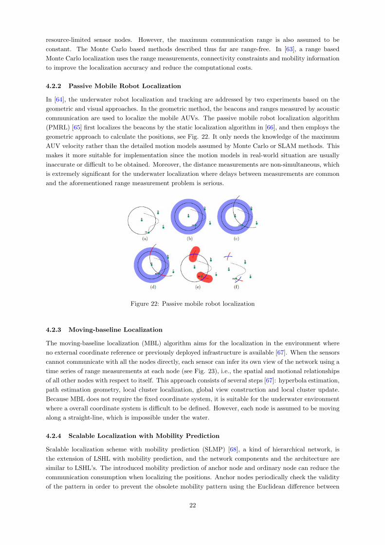
4.2.2 Passive Mobile Robot Localization

In [64], the underwater robot localization and tracking are addressed by two experiments based on the

geometric and visual approaches. In the geometric method, the beacons and ranges measured by acoustic

communication are used to localize the mobile AUVs. The passive mobile robot localization algorithm

(PMRL) [65] first localizes the beacons by the static localization algorithm in [66], and then employs the

geometric approach to calculate the positions, see Fig. 22. It only needs the knowledge of the maximum

AUV velocity rather than the detailed motion models assumed by Monte Carlo or SLAM methods. This

makes it more suitable for implementation since the motion models in real-world situation are usually

inaccurate or difficult to be obtained. Moreover, the distance measurements are non-simultaneous, which

is extremely significant for the underwater localization where delays between measurements are common

and the aforementioned range measurement problem is serious.

Figure 22: Passive mobile robot localization

4.2.3 Moving-baseline Localization

The moving-baseline localization (MBL) algorithm aims for the localization in the environment where

no external coordinate reference or previously deployed infrastructure is available [67]. When the sensors

cannot communicate with all the nodes directly, each sensor can infer its own view of the network using a

time series of range measurements at each node (see Fig. 23), i.e., the spatial and motional relationships

of all other nodes with respect to itself. This approach consists of several steps [67]: hyperbola estimation,

path estimation geometry, local cluster localization, global view construction and local cluster update.

Because MBL does not require the fixed coordinate system, it is suitable for the underwater environment

where a overall coordinate system is difficult to be defined. However, each node is assumed to be moving

along a straight-line, which is impossible under the water.

4.2.4 Scalable Localization with Mobility Prediction

Scalable localization scheme with mobility prediction (SLMP) [68], a kind of hierarchical network, is

the extension of LSHL with mobility prediction, and the network components and the architecture are

similar to LSHL’s. The introduced mobility prediction of anchor node and ordinary node can reduce the

communication consumption when localizing the positions. Anchor nodes periodically check the validity

of the pattern in order to prevent the obsolete mobility pattern using the Euclidean difference between

22

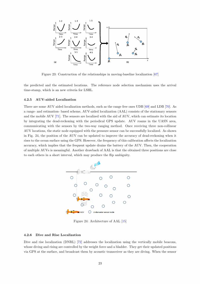
Figure 23: Construction of the relationships in moving-baseline localization [67]

the predicted and the estimated locations. The reference node selection mechanism uses the arrival

time-stamp, which is an new criteria for LSHL.

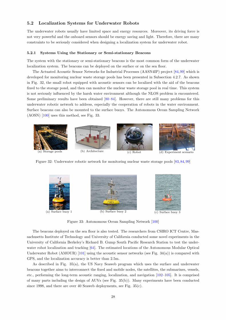
4.2.5 AUV-aided Localization

There are some AUV aided localization methods, such as the range free ones UDB [69] and LDB [70]. As

a range- and estimation- based scheme, AUV-aided localization (AAL) consists of the stationary sensors

and the mobile AUV [71]. The sensors are localized with the aid of AUV, which can estimate its location

by integrating the dead-reckoning with the periodical GPS update. AUV roams in the UASN area,

communicating with the sensors by the two-way ranging method. Once receiving three non-collinear

AUV locations, the static node equipped with the pressure sensor can be successfully localized. As shown

in Fig. 24, the position of the AUV can be updated to improve the accuracy of dead-reckoning when it

rises to the ocean surface using the GPS. However, the frequency of this calibration affects the localization

accuracy, which implies that the frequent update drains the battery of the AUV. Then, the cooperation

of multiple AUVs is meaningful. Another drawback of AAL is that the obtained three positions are close

to each others in a short interval, which may produce the flip ambiguity.

Figure 24: Architecture of AAL [15]

4.2.6 Dive and Rise Localization

Dive and rise localization (DNRL) [72] addresses the localization using the vertically mobile beacons,

whose diving and rising are controlled by the weight force and a bladder. They get their updated positions

via GPS at the surface, and broadcast them by acoustic transceiver as they are diving. When the sensor

23

nodes passively receive the DNR beacon messages, the range is measured by time of arrival under the

assumption that the nodes are synchronized. Then, the locations of the sensors are estimated using

either bounding box or triangulation algorithm. DNRL is a silent localization scheme and considers

the horizontal motion with the force of slow currents. On the other hands, a large number of DNR

beacons are needed for high localization success, and the time synchronization and Doppler effect affect

the performance. In order to enhance the the coverage of DNRL, the multi stage localization (MSL) [73]

employs the localized ordinary nodes as the beacon. It also uses the “Meandering Current Mobility with

Surface Effect model” to represent the mobility model of the underwater sensors when performing the

simulation. However, due to this iterative localization, MSL is high communication overhead and is much

energy consuming than DNRL. Moreover, MSL suffers from the error accumulation.

In [74], 3D multi-power area localization scheme (3D-MALS) that combines the area localization

scheme (ALS) [75] and DETL is proposed. It extends ALS to 3D by introducing the detachable elevator

transceivers in DETL, which can descend and ascend under the water.

4.2.7 Simultaneous Localization and Environmental Mapping

As a method which can concurrently estimate the location and build a map of the environment, Simultane-

ous Localization and Environmental Mapping (SLAM) has been widely used in robot localization [76,77].

Because the good performance of SLAM in reality, it is also introduced to the WSN. D. Marinakis et

al. [78] present an Expectation Maximization (EM) algorithm for simultaneously localizing the sensors and

mapping the environment. A prior probability distribution function (PDF) is built using the topographic

map and then it is refined by the other environmental measurements, such as salinity, temperature and

current velocity. The novelty of this method is to improve the WSN localization using the smoothly

varying parameters. In [79], the integration of underwater sensor networks and magnetometer is used for

silent localization. The moving trajectory of the vessel and the sensor locations are estimated using the

Extended Kalman Filter (EKF) based SLAM.

An underwater localization system for monitoring nuclear waste storage pool is proposed in [80–84].

The initial prototype of the AUV looks like a ball whose diameter is approximately 10cm (see Fig.25).

They are equipped with acoustic transmitter and receiver, which can be used to communicate with each

other and measure the distances. The architecture of the system is illustrated in Fig. 26. It can be

seen that the cluttered underwater environment is the primary challenge faced by this system since the

irregularly sharped obstacles produce many difficulties on the localization and environment mapping. In

order to address this Non-Line-Of-Sight (NLOS) problem, the convex programming based method [83]

and dynamic node placement [82] can be used.

Figure 25: A prototype robot [83]

Figure 26: Architecture of the system [81]

24

4.3 Localization for Mobile Swarm

As shown in Fig. 14, both of the beacons and the unknown nodes in the mobile swarm are mobile. It is

different from the aforementioned mobile network in the mobility of the anchors or sensors [85,86].

Mobile swarm is the general situation of WSN based localization and has several advantages:

� Its network coverage and flexibility are enhanced. The network coverage can be increased by the

mobility of the whole network, which can move to the interesting region without the constraint of

fixed static beacon. Therefore, it is a promising solution for the pelagic application although it

suffers from the execrable ocean environment and is constrained by the limited energy.

� It is efficient. Since the deployment of the fixed anchors or the date collection using the vessels are

time- and energy- consuming, and may be infeasible or undesirable in some cases, mobile swarm is

more efficient than the stationary and mobile networks.

� It is suitable for cooperation. Although the low ranging precision and the physical constraints of the

sensor nodes aggravate the difficulty of localization for mobile sensor nodes, the inherent character

of sharing information between many nodes enables the multiple sensors to complete the task by

cooperation.

However, mobile swarm is more complicated than the mobile networks, and encounters many tough

problems, such as the localizability. They became more difficult in the underwater environment because

of the long time delay of signal propagation, the disturbances of the wind and ocean current, etc.

4.3.1 Motion-Aware Self Localization

Motion-aware self-localization (MASL) which is appropriate for the offline applications saves the gathered

information for the posterior central processing when the mission ends [87]. It aims to accurately localize

the sensors by tackling the inaccurate distance measurements. As illustrated in Fig. 27, a swarm of

autonomous nodes which drift freely in the surveillance region collaborate with each other by acoustic

communication. A sensor prototype whose diameter is only 25cm is presented in Fig. 28. The factor

graph and the sum-product algorithm [88,89] are used to compute the position distribution of the mobile

sensors via message passing. The MASL highly reduces the computation and energy consumption of

the AUVs, and makes use of the inter-node distance constraints to improve the accuracy. However, it

cannot be used for the real-time application, which is its great weakness. Another drawback is the need of

synchronization and the frequent messaging for distance. The synchronization problem can be addressed

using the Sufficient Distance Map Estimation(SDME) [90], which is the improvement of MASL. Note

that both MASL and SDME have considered the ocean environment.

Figure 27: Motion-aware self-localization [87] Figure 28: A sensor prototype of MASL [91]

4.3.2 Collaborative Localization

As a prediction-based method, collaborative localization (CL) [92] is designed for a swarm of underwater

sensors which float freely with currents. It aims to determine the locations without prior planning or

pre-deployed infrastructure (e.g., long range transponders on surface buoys or ships). There are two types

of nodes diving vertically in the system: profiler and follower. The former is always much deeper than

25

the latter when descending. The position of profiler with respect to the followers is estimated using the

distances periodically measured using TOA, see Fig. 29. Since the nodes are assumed to move in the

same reference frame with the same speed, the position of the profiler can be a prediction of the future

locations of the followers. The required time synchronization and the disturbance of the ocean currents

are the serious influences of CL. Moreover, CL is not suitable for the applications in a large area due to

its mainly vertical data collection.

Figure 29: Trajectories of CL [92]

A cooperative localization scheme (CLS) is proposed in [93] for mobile swarm. It aims to estimate

the position and velocity of the unknown nodes given the distance measurement to the mobile beacons.

Its key point is to use the velocity estimation to assist the network localization because the velocities

provide useful information. An extended Kalman filter is introduced to fuse the estimated node position

with the node velocity estimation, improving the localization performance. The proposed algorithm is

also distributed, which is suitable for the mobile swarm. However, a drawback is the need of the Doppler

sensor, which increases the hardware cost and consumes more energy. The approach proposed in [94] can

overcome this problem.

4.3.3 Monte Carlo Localization

The third situation in [19] uses the Monte Carlo method described in Subsection 4.2.1 to address the

mobile swarm. The principle remains the same. According to the simulation results [19], the localization

accuracy is much better than Centroid and Amorphous methods. But the localization error increases as

the grow of the node speed.

4.4 Summary

In this section, many underwater localization algorithms are introduced according to the three different

categories. As a kind of relatively mature network, the stationary network has been widely investigated,

and there are many underwater localization methods specifically designed for it. In contrast, there are

lack of localization schemes for the mobile network and mobile swarm, and many challenging problems

still demand prompt solutions.

26

5 Existing Underwater Sensor Network Systems

As the increasing demand of the underwater applications, there are some off-the-shelf underwater testbeds

and systems. An online database lists more than 100 existing oceanic systems investigated by the different

research institutions and companies [95]. However, each system has its own advantages and disadvantages

due to the different purposes, performance requirements and application scenarios.

5.1 Traditional Underwater Positioning Systems

As the traditional underwater positioning systems, Long Baseline (LBL) system, Short Baseline (SBL)

system and Ultra Short Baseline (USBL) system have been widely used in various underwater applications,

especially for offshore oil and gas exploration. There are also many commercial systems of them, which

are summarized in [96] and [97].

As shown in Fig. 30(a), LBL employs the beacons deployed on the sea floor, the acoustic range

measurements and the trilateration method. It usually has high localization accuracy. However, the pre-

deployment of the beacons is time consuming and costly. Both SBL and USBL are ship-based positioning

systems, which use the transceiver attached on a pole under a ship instead of the sensors mounted on the

sea bottom, see Fig. 30(b) and Fig. 30(c). SBL requires three or more sonar transducers to perform the

localization, while USBL which introduces the signal run time and phase shift to measure the distance

and direction only needs a transducer array. As a successful commercial “underwater GPS” system,

NASNet which integrates these three kind of systems (see Fig. 31) has served the offshore industry since

2000.

However, the employed devices (beacons, sensors, ships, etc.) of these three methods tend to be energy

consuming, expensive and heavy, which means they are all unsuitable for the underwater localization of

robot.

(a) LBL (b) SBL (c) USBL

Figure 30: Baseline based underwater acoustic positioning systems

Figure 31: NASNet [98]

27

5.2 Localization Systems for Underwater Robots

The underwater robots usually have limited space and energy resources. Moreover, its driving force is

not very powerful and the onboard sensors should be energy saving and light. Therefore, there are many

constraints to be seriously considered when designing a localization system for underwater robot.

5.2.1 Systems Using the Stationary or Semi-stationary Beacons

The system with the stationary or semi-stationary beacons is the most common form of the underwater

localization system. The beacons can be deployed on the surface or on the sea floor.

The Actuated Acoustic Sensor Networks for Industrial Processes (AASN4IP) project [84,99] which is

developed for monitoring nuclear waste storage pools has been presented in Subsection 4.2.7. As shown

in Fig. 32, the small robot equipped with acoustic sensors can be localized with the aid of the beacons

fixed to the storage pond, and then can monitor the nuclear waste storage pool in real time. This system

is not seriously influenced by the harsh water environment although the NLOS problem is encountered.

Some preliminary results have been obtained [80–84]. However, there are still many problems for this

underwater robotic network to address, especially the cooperation of robots in the water environment.

Surface beacons can also be mounted to the surface buoys. The Autonomous Ocean Sampling Network

(AOSN) [100] uses this method, see Fig. 33.

(a) Storage pools (b) Architecture (c) Robot (d) Experiment scenario

Figure 32: Underwater robotic network for monitoring nuclear waste storage pools [83,84,99]

(a) Surface buoy 1 (b) Surface buoy 2 (c) Surface buoy 3

Figure 33: Autonomous Ocean Sampling Network [100]

The beacons deployed on the sea floor is also tested. The researchers from CSIRO ICT Centre, Mas-

sachusetts Institute of Technology and University of California conducted some novel experiments in the

University of California Berkeley’s Richard B. Gump South Pacific Research Station to test the under-

water robot localization and tracking [64]. The estimated locations of the Autonomous Modular Optical

Underwater Robot (AMOUR) [101] using the acoustic sensor networks (see Fig. 34(a)) is compared with

GPS, and the localization accuracy is better than 2.5m.

As described in Fig. 35(a), the US Navy Seaweb program which uses the surface and underwater

beacons together aims to interconnect the fixed and mobile nodes, the satellites, the submarines, vessels,

etc., performing the long-term acoustic ranging, localization, and navigation [102–105]. It is comprised

of many parts including the design of AUVs (see Fig. 35(b)). Many experiments have been conducted

since 1998, and there are over 40 Seaweb deployments, see Fig. 35(c).

28

(a) Beacon sensors (b) AMOUR and experiment scenario

Figure 34: Experiments with underwater robot localization and tracking [64]

(a) Architecture of Seaweb (b) SAUV (c) Beacon deployment

Figure 35: US Navy Seaweb program [102–105]

There are also some simulation and test tools for underwater sensor networks, such as the recent

Sapienza University Networking framework for underwater Simulation, Emulation and real-life Testing

(SUNSET) [106]. As shown in Fig. 36, it has been tested in reality although some other experiments are

still carrying out.

(a) Test1 (b) Test2(c) Test3

Figure 36: SUNSET [106]

5.2.2 Systems Without Static Beacon

However, almost all of the proposed UASN real systems perform the localization of the underwater robots

powered by the propeller with the aid of the stationary or semi-stationary anchored sensors. To the best

of our knowledge, MASL introduced in Subsection 4.3.1 is the only system which is tested in the actual

sea without fixed anchors [91]. The vehicles can be commanded to maintain the various specific depths

for a given amount of time in the trails. The experiment results verify the feasibility of this method.

5.2.3 Localization System for Robotic Fish

The localization of the robotic fish is the one where the underwater robot is not driven by the propeller.

Because the onboard resources of the robotic fish are more limited than the general AUV’s, the localization

29

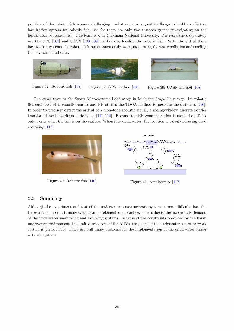
problem of the robotic fish is more challenging, and it remains a great challenge to build an effective

localization system for robotic fish. So far there are only two research groups investigating on the

localization of robotic fish. One team is with Chonnam National University. The researchers separately

use the GPS [107] and UASN [108, 109] methods to localize the robotic fish. With the aid of these

localization systems, the robotic fish can autonomously swim, monitoring the water pollution and sending

the environmental data.

Figure 37: Robotic fish [107] Figure 38: GPS method [107] Figure 39: UASN method [108]

The other team is the Smart Microsystems Laboratory in Michigan Stage University. Its robotic

fish equipped with acoustic sensors and RF utilizes the TDOA method to measure the distances [110].

In order to precisely detect the arrival of a monotone acoustic signal, a sliding-window discrete Fourier

transform based algorithm is designed [111, 112]. Because the RF communication is used, the TDOA

only works when the fish is on the surface. When it is underwater, the location is calculated using dead

reckoning [113].

Figure 40: Robotic fish [110] Figure 41: Architecture [112]

5.3 Summary

Although the experiment and test of the underwater sensor network system is more difficult than the

terrestrial counterpart, many systems are implemented in practice. This is due to the increasingly demand

of the underwater monitoring and exploring systems. Because of the constraints produced by the harsh

underwater environment, the limited resources of the AUVs, etc., none of the underwater sensor network

system is perfect now. There are still many problems for the implementation of the underwater sensor

network systems.

30

6 Conclusions

In this report, a survey is conducted to summarize the challenges, the state-of-the-art algorithms and

systems of underwater localization using WSN. First, several classic architectures and ranging methods

are introduced. Then, many underwater localization algorithms and existing systems are presented.

Although the WSN based underwater localization has been investigated for years, there are still many

challenging problems to be addressed, especially for the localization of the mobile networks and the mobile

swarm. The underwater localization of robotic fish is also more difficult than that of the common AUV

powered by the propeller.

31

References

[1] A. Khan and L. Jenkins, “Undersea wireless sensor network for ocean pollution prevention,” in 3rd International

Conference on Communication Systems Software and Middleware and Workshops. IEEE, 2008, pp. 2–8.

[2] Y. Huang, W. Liang, H. Yu, and Y. Xiao, “Target tracking based on a distributed particle filter in underwater sensor

networks,” Wireless Communications and Mobile Computing, vol. 8, no. 8, pp. 1023–1033, 2008.

[3] I. Akyildiz, D. Pompili, and T. Melodia, “Underwater acoustic sensor networks: research challenges,” Ad hoc networks,

vol. 3, no. 3, pp. 257–279, 2005.

[4] ——, “State-of-the-art in protocol research for underwater acoustic sensor networks,” in Proceedings of the 1st ACM

international workshop on Underwater networks. ACM, 2006, pp. 7–16.

[5] J. Leonard, A. Bennett, C. Smith, and H. Feder, “Autonomous underwater vehicle navigation,” in IEEE ICRA

Workshop on Navigation of Outdoor Autonomous Vehicles, 1998.

[6] X. Yun, E. Bachmann, R. McGhee, R. Whalen, R. Roberts, R. Knapp, A. Healey, and M. Zyda, “Testing and

evaluation of an integrated gps/ins system for small auv navigation,” IEEE Journal of Oceanic Engineering, vol. 24,

no. 3, pp. 396–404, 1999.

[7] H. Rice, S. Kelmenson, and L. Mendelsohn, “Geophysical navigation technologies and applications,” in Position

Location and Navigation Symposium. IEEE, 2004, pp. 618–624.

[8] M. Erol-Kantarci, H. Mouftah, and S. Oktug, “A survey of architectures and localization techniques for underwater

acoustic sensor networks,” Communications Surveys and Tutorials, vol. 13, no. 3, pp. 487–502, 2011.

[9] I. Akyildiz, D. Pompili, and T. Melodia, “Challenges for efficient communication in underwater acoustic sensor

networks,” ACM Sigbed Review, vol. 1, no. 2, pp. 3–8, 2004.

[10] I. Vasilescu, K. Kotay, D. Rus, M. Dunbabin, and P. Corke, “Data collection, storage, and retrieval with an underwater

sensor network,” in Proceedings of the 3rd international conference on Embedded networked sensor systems. ACM,

2005, pp. 154–165.

[11] V. Chandrasekhar, W. Seah, Y. Choo, and H. Ee, “Localization in underwater sensor networks: survey and chal-

lenges,” in Proceedings of the 1st ACM international workshop on Underwater networks. ACM, 2006, pp. 33–40.

[12] J. Heidemann, W. Ye, J. Wills, A. Syed, and Y. Li, “Research challenges and applications for underwater sensor

networking,” in Wireless Communications and Networking Conference, vol. 1. IEEE, 2006, pp. 228–235.

[13] M. Stojanovic, “Underwater wireless communications: current achievements and research challenges,” IEEE Oceanic

Engineering Society Newsletter, vol. 41, no. 2, 2006.

[14] J. Partan, J. Kurose, and B. Levine, “A survey of practical issues in underwater networks,” ACM SIGMOBILE

Mobile Computing and Communications Review, vol. 11, no. 4, pp. 23–33, 2007.

[15] M. Erol-Kantarci, H. Mouftah, and S. Oktug, “Localization techniques for underwater acoustic sensor networks,”

Communications Magazine, vol. 48, no. 12, pp. 152–158, 2010.

[16] H. Tan, R. Diamant, W. Seah, and M. Waldmeyer, “A survey of techniques and challenges in underwater localization,”

Ocean Engineering, vol. 38, no. 14, pp. 1663–1676, 2011.

[17] M. Erol-Kantarci, S. Oktug, L. Vieira, and M. Gerla, “Performance evaluation of distributed localization techniques

for mobile underwater acoustic sensor networks,” Ad Hoc Networks, vol. 9, no. 1, pp. 61–72, 2011.

[18] W. Liao, Y. Lee, and S. Kedia, “Mobile anchor positioning for wireless sensor networks,” IET Communications,

vol. 5, no. 7, pp. 914–921, 2011.

[19] L. Hu and D. Evans, “Localization for mobile sensor networks,” in Proceedings of the 10th annual international

conference on Mobile computing and networking. ACM, 2004, pp. 45–57.

[20] W. Lin, D. Li, Y. Tan, J. Chen, and T. Sun, “Architecture of underwater acoustic sensor networks: A survey,” in 1st

International Conference on Intelligent Networks and Intelligent Systems. IEEE, 2008, pp. 155–159.

[21] E. Cayirci, H. Tezcan, Y. Dogan, and V. Coskun, “Wireless sensor networks for underwater survelliance systems,”

Ad Hoc Networks, vol. 4, no. 4, pp. 431–446, 2006.

[22] J. Cui, J. Kong, M. Gerla, and S. Zhou, “The challenges of building mobile underwater wireless networks for aquatic

applications,” Network, IEEE, vol. 20, no. 3, pp. 12–18, 2006.

[23] X. Tan and J. Li, “Cooperative positioning in underwater sensor networks,” IEEE Transactions on Signal Processing,

vol. 58, no. 11, pp. 5860–5871, 2010.

[24] P. Etter, Underwater acoustic modeling and simulation. Taylor & Francis, 2003.

[25] Y. Xiao, Underwater acoustic sensor networks. Auerbach publications, 2009.

[26] F. Jensen, “Numerical models of sound propagation in real oceans,” in OCEANS 82. IEEE, 1982, pp. 147–154.

32

[27] D. McCrady, L. Doyle, H. Forstrom, T. Dempsey, and M. Martorana, “Mobile ranging using low-accuracy clocks,”

IEEE Transactions on Microwave Theory and Techniques, vol. 48, no. 6, pp. 951–958, 2000.

[28] M. Isik and O. Akan, “A three dimensional localization algorithm for underwater acoustic sensor networks,” IEEE

Transactions on Wireless Communications, vol. 8, no. 9, pp. 4457–4463, 2009.

[29] C. Wang and L. Xiao, “Sensor localization under limited measurement capabilities,” IEEE Network, vol. 21, no. 3,

pp. 16–23, 2007.

[30] X. Sheng and Y. Hu, “Maximum likelihood multiple-source localization using acoustic energy measurements with

wireless sensor networks,” IEEE Transactions on Signal Processing, vol. 53, no. 1, pp. 44–53, 2005.

[31] M. Noel, P. Joshi, and T. Jannett, “Improved maximum likelihood estimation of target position in wireless sensor

networks using particle swarm optimization,” in 3rd International Conference on Information Technology: New

Generations. IEEE, 2006, pp. 274–279.

[32] N. Patwari, A. Hero III, M. Perkins, N. Correal, and R. O’dea, “Relative location estimation in wireless sensor

networks,” IEEE Transactions on Signal Processing, vol. 51, no. 8, pp. 2137–2148, 2003.

[33] R. Zemek, S. Hara, K. Yanagihara, and K. Kitayama, “A joint estimation of target location and channel model

parameters in an ieee 802.15. 4-based wireless sensor network,” in 18th International Symposium on Personal, Indoor

and Mobile Radio Communications. IEEE, 2007, pp. 1–5.

[34] K. Whitehouse and D. Culler, “A robustness analysis of multi-hop ranging-based localization approximations,” in

Proceedings of the 5th international conference on Information processing in sensor networks. ACM, 2006, pp.

317–325.

[35] Y. Shang, W. Ruml, Y. Zhang, and M. Fromherz, “Localization from mere connectivity,” in Proceedings of the 4th

ACM international symposium on Mobile ad hoc networking and computing. ACM, 2003, pp. 201–212.

[36] Y. Shang, W. Rumi, Y. Zhang, and M. Fromherz, “Localization from connectivity in sensor networks,” IEEE Trans-

actions on Parallel and Distributed Systems, vol. 15, no. 11, pp. 961–974, 2004.

[37] P. Biswas and Y. Ye, “Semidefinite programming for ad hoc wireless sensor network localization,” in Proceedings of

the 3rd international symposium on Information processing in sensor networks. ACM, 2004, pp. 46–54.

[38] P. Biswas, T. Liang, K. Toh, Y. Ye, and T. Wang, “Semidefinite programming approaches for sensor network localiza-

tion with noisy distance measurements,” IEEE Transactions on Automation Science and Engineering, vol. 3, no. 4,

pp. 360–371, 2006.

[39] A. Savvides, C. Han, and M. Strivastava, “Dynamic fine-grained localization in ad-hoc networks of sensors,” in

Proceedings of the 7th annual international conference on Mobile computing and networking. ACM, 2001, pp.

166–179.

[40] X. Cheng, H. Shu, Q. Liang, and D. Hung-Chang Du, “Silent positioning in underwater acoustic sensor networks,”

IEEE Transactions on Vehicular Technology, vol. 57, no. 3, pp. 1756–1766, 2008.

[41] H. Tan, Z. Eu, and W. Seah, “An enhanced underwater positioning system to support deepwater installations,” in

OCEANS 2009, MTS/IEEE Biloxi-Marine Technology for Our Future: Global and Local Challenges. IEEE, 2009,

pp. 1–8.

[42] H. Tan, A. Gabor, Z. Eu, and W. Seah, “A wide coverage positioning system (wps) for underwater localization,” in

2010 IEEE International Conference on Communications (ICC). IEEE, 2010, pp. 1–5.

[43] T. Bian, R. Venkatesan, and C. Li, “Design and evaluation of a new localization scheme for underwater acoustic

sensor networks,” in Global Telecommunications Conference. IEEE, 2009, pp. 1–5.

[44] ——, “An improved localization method using error probability distribution for underwater sensor networks,” in 2010

IEEE International Conference on Communications (ICC). IEEE, 2010, pp. 1–6.

[45] A. Othman, A. Adams, and C. Tsimenidis, “Node discovery protocol and localization for distributed underwater

acoustic networks,” in International Conferenceon Internet and Web Applications and Services/Advanced Interna-

tional Conference on Telecommunications. IEEE, 2006, pp. 93–93.

[46] A. Othman, “Gps-less localization protocol for underwater acoustic networks,” in 5th IFIP International Conference

on Wireless and Optical Communications Networks. IEEE, 2008, pp. 1–6.

[47] C. Tian, W. Liu, J. Jin, Y. Wang, and Y. Mo, “Localization and synchronization for 3d underwater acoustic sensor

networks,” Ubiquitous Intelligence and Computing, pp. 622–631, 2007.

[48] Z. Zhou, J. Cui, and S. Zhou, “Efficient localization for large-scale underwater sensor networks,” Ad Hoc Networks,

vol. 8, no. 3, pp. 267–279, 2010.

[49] K. Chen, Y. Zhou, and J. He, “A localization scheme for underwater wireless sensor networks,” International Journal

of Advanced Science and Technology, vol. 4, 2009.

33

[50] A. Teymorian, W. Cheng, L. Ma, X. Cheng, X. Lu, and Z. Lu, “3d underwater sensor network localization,” IEEE

Transactions on Mobile Computing, vol. 8, no. 12, pp. 1610–1621, 2009.

[51] W. Cheng, A. Teymorian, L. Ma, X. Cheng, X. Lu, and Z. Lu, “Underwater localization in sparse 3d acoustic sensor

networks,” in 27th Conference on Computer Communications. IEEE, 2008, pp. 236–240.

[52] W. Cheng, A. Thaeler, X. Cheng, F. Liu, X. Lu, and Z. Lu, “Time-synchronization free localization in large scale

underwater acoustic sensor networks,” in 29th IEEE International Conference on Distributed Computing Systems

Workshops. IEEE, 2009, pp. 80–87.

[53] A. Coppens, “Simple equations for the speed of sound in neptunian waters,” The Journal of the Acoustical Society

of America, vol. 69, p. 862, 1981.

[54] S. Tilak, V. Kolar, N. Abu-Ghazaleh, and K. Kang, “Dynamic localization control for mobile sensor networks,” in

24th IEEE International Conference on Performance, Computing, and Communications. IEEE, 2005, pp. 587–592.

[55] N. Ahmed, M. Rutten, T. Bessell, S. Kanhere, N. Gordon, and S. Jha, “Detection and tracking using particle-filter-

based wireless sensor networks,” IEEE Transactions on Mobile Computing, vol. 9, no. 9, pp. 1332–1345, 2010.

[56] X. Wang, M. Fu, and H. Zhang, “Target tracking in wireless sensor networks based on the combination of kf and mle

using distance measurements,” IEEE Transactions on Mobile Computing, no. 99, pp. 1–1, 2011.

[57] J. Djugash, S. Singh, and P. Corke, “Further results with localization and mapping using range from radio,” in Field

and Service Robotics. Springer, 2006, pp. 231–242.

[58] F. Dellaert, D. Fox, W. Burgard, and S. Thrun, “Monte carlo localization for mobile robots,” in 1999 IEEE Interna-

tional Conference on Robotics and Automation, vol. 2. IEEE, 1999, pp. 1322–1328.

[59] A. Doucet, S. Godsill, and C. Andrieu, “On sequential monte carlo sampling methods for bayesian filtering,” Statistics

and computing, vol. 10, no. 3, pp. 197–208, 2000.

[60] J. Sheu, W. Hu, and J. Lin, “Distributed localization scheme for mobile sensor networks,” IEEE Transactions on

Mobile Computing, vol. 9, no. 4, pp. 516–526, 2010.

[61] M. Rudafshani and S. Datta, “Localization in wireless sensor networks,” in 6th International Symposium on Infor-

mation Processing in Sensor Networks. IEEE, 2007, pp. 51–60.

[62] A. Baggio and K. Langendoen, “Monte carlo localization for mobile wireless sensor networks,” Ad Hoc Networks,

vol. 6, no. 5, pp. 718–733, 2008.

[63] B. Dil, S. Dulman, and P. Havinga, “Range-based localization in mobile sensor networks,” Wireless Sensor Networks,

pp. 164–179, 2006.

[64] P. Corke, C. Detweiler, M. Dunbabin, M. Hamilton, D. Rus, and I. Vasilescu, “Experiments with underwater robot

localization and tracking,” in 2007 IEEE International Conference on Robotics and Automation. IEEE, 2007, pp.

4556–4561.

[65] C. Detweiler, J. Leonard, D. Rus, and S. Teller, “Passive mobile robot localization within a fixed beacon field,”

Algorithmic Foundation of Robotics VII, pp. 425–440, 2008.

[66] D. Moore, J. Leonard, D. Rus, and S. Teller, “Robust distributed network localization with noisy range measure-

ments,” in Proceedings of the 2nd international conference on Embedded networked sensor systems. ACM, 2004,

pp. 50–61.

[67] J. Park, E. Demaine, and S. Teller, “Moving-baseline localization,” in International Conference on Information

Processing in Sensor Networks. IEEE, 2008, pp. 15–26.

[68] Z. Zhou, Z. Peng, J. Cui, Z. Shi, and A. Bagtzoglou, “Scalable localization with mobility prediction for underwater

sensor networks,” IEEE Transactions on Mobile Computing, pp. 335–348, 2010.

[69] H. Luo, Y. Zhao, Z. Guo, S. Liu, P. Chen, and L. Ni, “Udb: using directional beacons for localization in underwater

sensor networks,” in 14th IEEE International Conference on Parallel and Distributed Systems. IEEE, 2008, pp.

551–558.

[70] H. Luo, Z. Guo, W. Dong, F. Hong, and Y. Zhao, “Ldb: Localization with directional beacons for sparse 3d underwater

acoustic sensor networks,” Journal of Networks, vol. 5, no. 1, pp. 28–38, 2010.

[71] M. Erol, L. Vieira, and M. Gerla, “Auv-aided localization for underwater sensor networks,” in International Confer-

ence on Wireless Algorithms, Systems and Applications. IEEE, 2007, pp. 44–54.

[72] ——, “Localization with dive’n’rise (dnr) beacons for underwater acoustic sensor networks,” in Proceedings of the

second workshop on Underwater networks. ACM, 2007, pp. 97–100.

[73] M. Erol, L. Vieira, A. Caruso, F. Paparella, M. Gerla, and S. Oktug, “Multi stage underwater sensor localization

using mobile beacons,” in 2nd International Conference on Sensor Technologies and Applications. IEEE, 2008, pp.

710–714.

34

[74] Y. Zhou, J. He, K. Chen, J. Chen, and A. Liang, “An area localization scheme for large scale underwater wireless

sensor networks,” in International Conference on Communications and Mobile Computing, vol. 1. IEEE, 2009, pp.

543–547.

[75] V. Chandrasekhar and W. Seah, “An area localization scheme for underwater sensor networks,” in OCEANS 2006-

Asia Pacific. IEEE, 2007, pp. 1–8.

[76] S. Williams and I. Mahon, “Simultaneous localisation and mapping on the great barrier reef,” in 2004 IEEE Inter-

national Conference on Robotics and Automation, vol. 2. IEEE, 2004, pp. 1771–1776.

[77] M. Walter, F. Hover, and J. Leonard, “Slam for ship hull inspection using exactly sparse extended information filters,”

in 2008 IEEE International Conference on Robotics and Automation. IEEE, 2008, pp. 1463–1470.

[78] D. Marinakis, N. MacMillan, R. Allen, and S. Whitesides, “Simultaneous localization and environmental mapping

with a sensor network,” in 2011 IEEE International Conference on Robotics and Automation. IEEE, 2011, pp.

5881–5886.

[79] C. Jonas, S. Martin, and G. Fredrik, “Silent localization of underwater sensors using magnetometers,” EURASIP

Journal on Advances in Signal Processing, vol. 2010, 2010.

[80] S. Nawaz, M. Hussain, S. Watson, N. Trigoni, and P. Green, “An underwater robotic network for monitoring nuclear

waste storage pools,” Sensor Systems and Software, pp. 236–255, 2010.

[81] M. Hussain and N. Trigoni, “Distributed localization in cluttered underwater environments,” in Proceedings of the

5th ACM International Workshop on Underwater Networks. ACM, 2010, p. 8.

[82] ——, “Dynamic node placement for multi-hop localization in cluttered environments,” in 8th Annual IEEE Commu-

nications Society Conference on Sensor, Mesh and Ad Hoc Communications and Networks, 2011.

[83] S. Nawaz and N. Trigoni, “Convex programming based robust localization in nlos prone cluttered environments,” in

10th International Conference onInformation Processing in Sensor Networks. IEEE, 2011, pp. 318–329.

[84] P. G. M. H. S. N. A. P. Z. Q. S. S. N. T. S. W. T.A. York, P.N. Green, “Acoustic sensor networks for decommissioning,”

Measurement and Control, vol. 45, no. 3, pp. 48–54, 2012.

[85] H. Bao, B. Zhang, C. Li, and Z. Yao, “Mobile anchor assisted particle swarm optimization (pso) based localization

algorithms for wireless sensor networks,” Wireless Communications and Mobile Computing, 2011.

[86] C. Ou, “A localization scheme for wireless sensor networks using mobile anchors with directional antennas,” IEEE

Sensors Journal, no. 99, pp. 1–1, 2011.

[87] D. Mirza and C. Schurgers, “Motion-aware self-localization for underwater networks,” in Proceedings of the 3rd ACM

international workshop on Underwater Networks. ACM, 2008, pp. 51–58.

[88] F. Kschischang, B. Frey, and H. Loeliger, “Factor graphs and the sum-product algorithm,” IEEE Transactions on

Information Theory, vol. 47, no. 2, pp. 498–519, 2001.

[89] H. Loeliger, “An introduction to factor graphs,” IEEE Signal Processing Magazine, vol. 21, no. 1, pp. 28–41, 2004.

[90] D. Mirza and C. Schurgers, “Energy-efficient ranging for post-facto self-localization in mobile underwater networks,”

IEEE Journal on Selected Areas in Communications, vol. 26, no. 9, pp. 1697–1707, 2008.

[91] J. Jaffe and C. Schurgers, “Sensor networks of freely drifting autonomous underwater explorers,” in Proceedings of

the 1st ACM international workshop on Underwater networks. ACM, 2006, pp. 93–96.

[92] D. Mirza and C. Schurgers, “Collaborative localization for fleets of underwater drifters,” in OCEANS 2007. IEEE,

2007, pp. 1–6.

[93] L. Dong, “Cooperative network localization via node velocity estimation,” in Wireless Communications and Net-

working Conference. IEEE, 2009, pp. 1–6.

[94] H. Rad, T. van Waterschoot, and G. Leus, “Anchorless cooperative localization for mobile wireless sensor networks,”

in Proceedings of Symposium on Information Theory Signal Process. IEEE, 2011, p. 916.

[95] [Online]. Available: http://auvac.org/people-organizations

[96] [Online]. Available: http://www.hydro-international.com/productsurvey/id12-Long Baseline Systems.html

[97] [Online]. Available: http://www.hydro-international.com/productsurvey/id13-UltraShort Baseline Systems.html

[98] [Online]. Available: http://www.nautronix.com/

[99] [Online]. Available: http://www.aasn4ip.org.uk/

[100] [Online]. Available: http://www.mbari.org/aosn/

[101] [Online]. Available: http://groups.csail.mit.edu/drl/underwater robotics/amour/amour.html

[102] J. Rice, B. Creber, C. Fletcher, P. Baxley, K. Rogers, K. McDonald, D. Rees, M. Wolf, S. Merriam, R. Mehio et al.,

“Evolution of seaweb underwater acoustic networking,” in Oceans 2000 MTS/IEEE Conference and Exhibition, vol. 3.

IEEE, 2000, pp. 2007–2017.

35

[103] J. Rice, “Undersea networked acoustic communication and navigation for autonomous mine-countermeasure systems,”

in Proceedings of the 5th International Symposium on Technology and the Mine Problem, 2002.

[104] ——, “Seaweb acoustic communication and navigation networks,” in Proceedings of the International Conference on

Underwater Acoustic Measurements: Technologies and Results, 2005.

[105] J. Rice and D. Green, “Underwater acoustic communications and networks for the us navy’s seaweb program,” in

Second International Conference on Sensor Technologies and Applications. IEEE, 2008, pp. 715–722.

[106] [Online]. Available: http://reti.dsi.uniroma1.it/UWSN Group/index.php?page=home

[107] D. Shin, S. Na, J. KIM, S. Baek, M. Song, A. Park, and S. KOREA, “Development of a gps-based autonomous

water pollution monitoring system using fish robots,” in Proceedings of the 6th WSEAS international conference on

Computational intelligence, man-machine systems and cybernetics. World Scientific and Engineering Academy and

Society (WSEAS), 2007, pp. 156–161.

[108] D. Shin, S. Na, J. Kim, and S. Baek, “Sonar localization using ubiquitous sensor network for water pollution monitoring

fish robots,” in 2007 IEEE International Symposium on Signal Processing and Information Technology. IEEE, 2007,

pp. 80–85.

[109] ——, “Fish robots for water pollution monitoring using ubiquitous sensor networks with sonar localization,” in

International Conference on Convergence Information Technology. IEEE, 2007, pp. 1298–1303.

[110] S. Shatara, X. Tan, E. Mbemmo, N. Gingery, and S. Henneberger, “Experimental investigation on underwater acoustic

ranging for small robotic fish,” in 2008 IEEE International Conference on Robotics and Automation. IEEE, 2008,

pp. 712–717.

[111] S. Shatara and X. Tan, “A compensated sliding-window dft algorithm for fine-grained underwater acoustic ranging,”

in IEEE/RSJ International Conference on Intelligent Robots and Systems. IEEE, 2009, pp. 4054–4059.

[112] ——, “An efficient, time-of-flight-based underwater acoustic ranging system for small robotic fish,” IEEE Journal of

Oceanic Engineering, vol. 35, no. 4, pp. 837–846, 2010.

[113] X. Tan, “Autonomous robotic fish as mobile sensor platforms: Challenges and potential solutions,” Marine Technology

Society Journal, vol. 45, no. 4, pp. 31–40, 2011.

36