Winter heating effects on plants performances, growth and ...
91
2020 UNIVERSIDADE DE LISBOA FACULDADE DE CIÊNCIAS DEPARTAMENTO DE BIOLOGIA ANIMAL WINTER HEATING EFFECTS ON PLANTS PERFORMANCES, GROWTH AND PHENOLOGY Liliana Scapucci Mestrado em Ecologia e Gestão Ambiental Relatório de Estágio orientado por: Cristina Branquinho Anders Ræbild
Transcript of Winter heating effects on plants performances, growth and ...
2020
UNIVERSIDADE DE LISBOA
FACULDADE DE CIÊNCIAS
DEPARTAMENTO DE BIOLOGIA ANIMAL
WINTER HEATING EFFECTS ON PLANTS PERFORMANCES,
GROWTH AND PHENOLOGY
Liliana Scapucci
Mestrado em Ecologia e Gestão Ambiental
Relatório de Estágio orientado por:
Cristina Branquinho
Anders Ræbild

i
Abstract
Climate change is unprecedently threating living organisms. The increasing of carbon dioxide in
the atmosphere is the major driver of climate change, causing a dramatic rise of temperature. Global
warming and high CO2 concentration have significant consequences on plants performances. Most
of the studies focus on the effect of climate change on growing season, since photosynthesis during
winter is negligible. However, mild winters are becoming more frequent and plants performances
could become more noteworthy. At high-latitudes where milder winters are linked to wider cloud
cover plants respiration could exceed photosynthesis causing a negative carbon balance.
Nonetheless, temperature rise during winter could affect growth and phenology leading to less carbon
storage and phenological mismatches. To understand plants performances, growth and phenology
under mild winter five species of seedlings (Picea abies, Abies alba, Larix X eurolepis, Fagus
sylvatica and Quercus robur) were set under different temperature and light treatments indoor and
outdoor for one month between January and February. Plants performances were measured on
evergreen conifers during the whole month. An increased level of dark respiration and a lower carbon
uptake was found in plants exposed to warmer temperatures. Growth and phenology were monitored
on the five species revealing species-specific responses. An overall advancement in phenology was
observed in plants placed at warmer temperatures. Light treatments triggered a phenology
advancement in Picea abies and Quercus robur. This study evidences the importance of including
winter temperatures and light to calculate annual carbon balance, and plants growth and phenology.
Keywords: winter photosynthesis • global warming • conifer respiration • carbon uptake •
phenological advancement
ii
Resumo
As alterações climáticas são uma das principais ameaças à sobrevivência de várias espécies. Estima-
se que a temperatura média da superfície da Terra aumente 1.5ºC entre os anos de 2030-2050. Prevê-se
que esta temperatura aumente especialmente em latitudes mais altas, atingindo mais 4.5ºC. Além disso,
o aumento do dióxido de carbono atmosférico está a alterar os ciclos de carbono, levando a
consequências que são altamente complexas de assimilar. As florestas representam um papel
fundamental para os ciclos gasosos, sendo um dos maiores sumidouros de carbono do planeta. Como o
desempenho das plantas pode ser afetado por elevadas temperaturas e por elevadas concentrações de
CO2, há incertezas sobre a conservação das florestas como sumidouros de carbono, sem que as mesmas
se tornem fontes de carbono. Assim sendo, pode eventualmente verificar-se um efeito reverso no papel
das florestas sob resultado do aquecimento global.
A fotossíntese é o único processo que converte energia solar, dióxido de carbono e água em
carboidratos não estruturais e oxigénio molecular. Desta forma, a energia solar é convertida em energia
química, que pode ser utilizada por organismos heterotróficos como fonte primária de alimento. A
fotossíntese é fortemente influenciada pelo ambiente, uma vez que esta responde a fatores ambientais
como luz, concentrações de CO2 e temperatura. Entre eles, o efeito da temperatura é particularmente
interessante porque envolve alterações em todas as etapas da fotossíntese.
A temperatura é um fator capaz de alterar as atividades das enzimas da cadeia da fotossíntese, criando
respostas amplas e diferentes. No entanto, não é apenas a temperatura que leva a impactos consideráveis
ao nível da fotossíntese. A luz é a responsável por fornecer a energia necessária para o processo
fotossintético, desempenhando por isso um papel altamente importante no desempenho das plantas. O
espectro de luz que pode ser usado pelas plantas para fazer a fotossíntese é chamado de radiação
fotossinteticamente ativa (PAR).
No contexto do presente estudo, as temperaturas mais elevadas estão principalmente associadas a
clima nublado, o que modifica a PAR. Esta diminui com condições de nebulosidade considerável, o que
corresponde a uma consequente diminuição da taxa de transpiração e aumento da taxa de fixação de
dióxido de carbono.
Temperatura e radiação luminosa são dois fatores altamente importantes a serem observados no
cenário de mudanças climáticas. Como consequência, a combinação destes dois fatores mostra respostas
complexas nas plantas, podendo não só afetar o desempenho das mesmas no inverno, mas também
influenciar o processo normal do seu crescimento e da sua fenologia. A monitorização destes dois
parâmetros e o estudo dos seus efeitos no desempenho da fotossíntese e, consequentemente, no
desenvolvimento das plantas, é crucial para entender os verdadeiros efeitos das alterações climáticas a
nível global.
O presente estudo pretende explorar esta temática, de forma a contribuir para a compreensão dos
efeitos do aquecimento global, no inverno, em cinco espécies de árvores que estão amplamente
distribuídas pela Europa: Picea abies, Abies alba, Larix X eurolepis, Fagus sylvatica e Quercus robur.
As experiências decorreram em Horshlom, Dinamarca.
Dois processos experimentais foram montados, de forma a expor as respetivas plantas a um ambiente
com temperaturas acima do normal, durante o período de 1 mês. Por um lado, pretendia-se testar a

iii
resposta das plantas num ambiente natural com um ligeiro, mas significativo, aumento de
temperatura, por outro, pretendia-se tornar essas condições extremas, através de criação de um
ambiente controlado e manipulável. Assim, 320 plantas foram selecionadas aleatoriamente para uma
experiência ao ar livre e 168 para uma experiência em ambiente fechado.
Ao ar livre foram preparadas 8 parcelas de 12 m2, onde metade delas foi aquecida com 6
aquecedores e a outra metade funcionou como controlo. Metade de cada parcela foi ainda coberta
com uma rede para reter 60% da luz e criar um ambiente de sombra. Pretendia-se manter as parcelas
aquecidas a 4ºC em comparação com o controlo, utilizando um computador capaz de manter a
diferença constante ao longo do tempo.
Na experiência em ambiente fechado, colocaram-se as plantas em quatro estufas diferentes e uma
parcela de controlo externa. As estufas foram aquecidas a uma temperatura média de 13°C - 11°C -
9°C - 6°C. Em cada estufa foram simulados ambientes diferentes: metade das plantas recebeu um
nível de luz ambiente e a outra metade foi isolada de fatores luminosos.
A experiência ocorreu de 7 de janeiro a 7 de fevereiro. Durante o mês experimental, foram
realizadas medições de trocas gasosas com CIRAS-3 em coníferas perenes (Picea abies e Abies
alba), ou seja, foram realizadas curvas de temperatura e luz, medição de luz ambiente e curvas
diurnas todas as semanas durante quatro semanas.Após o mês experimental, as plantas foram
movidas para um terreno ao ar livre e outro interno, numa estufa mais fria (respetivamente para as
plantas pertencentes ao experimento ao ar livre e ao experimento interior). Estas foram colocadas
aleatoriamente para o começo da estação de crescimento. Durante a primavera, efetuaram-se
medições de crescimento e de fenologia. Para a avaliação do crescimento, a altura e o diâmetro foram
medidos antes e depois da estação de crescimento, enquanto que a fenologia foi medida através de
métodos de pontuação durante a primavera.
Numa primeira análise, foi possível avaliar que a diferença de temperatura entre as parcelas
aquecidas e as de controlo, na experiência ao ar livre, foi de apenas 1,9°C. Foi também possível
demonstrar que os resultados foram menos significativos ao ar livre do que na experiência em estufas,
onde as temperaturas estabelecidas conseguiam ser facilmente alcançadas.
A análise estatística dos dados de trocas gasosas revelou um forte efeito da temperatura no
desempenho das plantas. As curvas de temperatura e de luz evidenciaram que as plantas implantadas
em ambientes mais frios apresentaram melhor desempenho do que as demais, e os níveis de
respiração em zonas de luminosidade reduzida aumentou em ambos os tratamentos de temperatura.
Dentro dos modelos criados para as respirações com luminosidade reduzida, verificou-se que,
especialmente na experiência interna, a respiração estava a aumentar exponencialmente com o efeito
do aumento de temperatura. Além disso, verificou-se também que a espécie Picea abies teve uma
taxa respiratória mais alta do que a espécie Abies alba.
A absorção de carbono também foi afetada pela temperatura. Foi possível notar uma diminuição
exponencial da fixação de carbono com o aumento da temperatura na experiência interna. Por sua
vez, as plantas colocadas em temperaturas mais elevadas durante o inverno tiveram uma menor
absorção de carbono. Além disso, as plantas que cresceram em temperaturas mais elevadas
mostraram uma maior diversidade e complexidade de respostas, o que significa que a variabilidade
parece aumentar com a temperatura. Por este motivo, prever a precisão das respostas das plantas a
temperaturas mais altas irá tornar-se cada vez mais complexo e incerto a longo prazo.
iv
Finalmente, foi efetuada uma análise do efeito dos tratamentos de temperatura e luz no crescimento
e fenologia das plantas. Os resultados mostraram que as respostas são altamente específicas e intrínsecas
de cada espécie. Algumas das espécies conseguiram beneficiar de temperaturas mais altas enquanto que
outras se mostraram mais afetadas. O Larix X eurolepis foi afetado negativamente pela temperatura, ao
contrário do Fagus sylvatica, que aumentou o seu crescimento quando exposto a tratamentos mais
quentes. A luz afetou diferencialmente o Quercus robur, onde este cresceu mais quando exposto à luz
ambiente dentro das estufas, e menos ao ar livre. Tudo isto veio suportar a ideia de que as respostas das
plantas podem variar significativamente dependendo das diferentes condições a que são submetidas.
Foi possível adequar modelos fenológicos apenas para a o ensaio interno. Infelizmente, a
generalização de dados do ensaio ao ar livre não permitiu uma análise precisa, por isso não foi possível
avaliar a fenologia dessas plantas. Além disso, as plantas instaladas em estufas evidenciaram um avanço
em eventos de primavera, quando expostas a temperaturas mais elevadas no inverno. Em especial,
Quercus robur e Picea abies tiveram cerca de 14 dias de avanço entre o tratamento mais quente e o mais
frio. O tratamento com luz teve um efeito sobre Quercus robur e Picea abies, onde ambos responderam
negativamente à ausência de luz durante o mês experimental com um atraso geral dos eventos de
primavera.
Para concluir, foram observados efeitos da temperatura no desempenho das plantas durante o inverno
e no crescimento e fenologia durante a primavera. Assim sendo, os dados correspondentes às
performances de plantas em invernos amenos devem ser incluídos nos estudos de modelos do balanço
anual de carbono e, as incompatibilidades de crescimento e fenologia deverão ser esperadas em cenários
de aquecimento global. As entidades responsáveis pela tomada de decisões a nível mundial devem levar
em consideração tais resultados, de forma a melhorar as práticas de gestão florestal e tentar combater
assim os efeitos adversos das alterações climáticas.
Palavras-chave: fotossíntese de inverno • aquecimento global • respiração de coníferas • absorção de
carbono • avanço fenológico

v
Acknowledgment
I want to thank Anders Rӕbild for letting me take part in this beautiful project, thanks for your
kindness and patience. You motivated the team with your passion, and you took care for each of us.
Thanks for all the things I learned about plant physiology and statistics, and thanks for having taught
me all practical tasks like drilling wood boards, screwing the heaters and fixing electronic devices. I
really appreciated your trust in me from the beginning. Besides, I must thank you for all the support
that I received in the faculty, I felt always welcomed, and I really valued your caring during the
pandemic that we had to face in the last part of the project.
A special thanks to my colleagues Anja Petek and Peter Petrík. The field work experience with
you was amazing, I learned so much from you. We worked hard together, but you always found a
moment for a joke and genuine laughs. You made me find the strength to wake up at 4 a.m. and to
take measurements the whole day despite the tiredness and the bad weather, we worked as a real
team. I will never forget this experience, you guys became friends more than colleagues, and I must
say that you are very passionate scientists. Thanks to all the people working at the Arboretum, thanks
for your help with plants caring and for your availability for everything we might have needed.
I thank my supervisor Cristina Branquinho for the support and the motivation you gave me despite
the busy schedule. Thanks to my co-supervisor Ana Luz, with your hints, availability and kindness,
you helped me since the first day I was looking for a project.
A very special thanks to my friends and buddies at the faculty Valeria Mazzola and Anna
Mariager Behrend. Valeria, thanks for your generous help in the field for the phenological
measurements and the continuous support with data analysis on R and the writing of my thesis. Thank
you for being always present in each day of my Danish experience inside and outside the faculty,
your friendship has been a certainty for me. Thank you, Anna for being so welcoming with me since
the first day in the office, thanks for your help in the field and the support in the thesis. You are my
first Danish friend, and I know this will last. Thank you, girls, for reading through my thesis and for
the beautiful and passionate conversations about it.
Thank you so much Chiara Modolo for the amazing illustrations. You are an amazing artist and
a person I can always count on for everything. Thank you Telma Figueiredo and Vera Pinheiro for
your help with the translations in Portuguese, thank you for your kindness and availability. Thanks
to my cousins Sere and Vale, and my friend Lalla for the hints on mathematics, R studio and statistical
analysis. Thanks, Dado, for your patience and help with the final steps of the thesis.
I want to thank all the friends I met in Copenhagen, you made this experience so special and
diverse from everything else. Thanks for being there in such a difficult year, thanks for all the
amazing conversations and laughs. You have been a family for me. I want to thank all the amazing
people that I met in Lisbon, in particular, Telma and Vitória,I could not have achieved this without
you and your will to work with me in English, you are very special friends.
Thanks to all the biologists that I met on my academic record, thanks for the passionate
conversations about this subject, a special thanks to Costi, Marem and Vale. A sincere thanks to all
the people who raised my interest in science. Thanks to Miki to motivate and support me during my
whole academic record and to always encourage me to venture. Thanks to all my Italian buddies, you

vi
are always there anywhere I move, supportive and nice no matter what, especially you, girls, Stefy and
Marga. A lot of thanks to the new friends that I met travelling in such an exceptional summer.
Finally, I want to thank with all my heart my family. My grandparents, nonna Bianca and nonno
Angelo, who are always there with infinite love, and a genuine passion for what I do although it is
difficult for you to understand it. Thank you to Lori, Luigi and Andrea for everything, we are an
exceptional but amazing family, thanks for being there and to guide and support my crazy choices. You
all are always there besides the kilometres that part us.
vii
Motivation
It was the beginning of March 2018, my last day of internship in Magoodhoo, Maldives. I was
swimming with my closest buddies observing the seabed in the shallow waters of Indian ocean during
the sunrise. The atmosphere was just incredible. The night before, we had the chance to see an
amazing documentary – Chasing Corals – made by Jeff Orlowski. The documentary told about the
heatwaves of 2015-2016 that killed a big portion of coral reefs all around the world. The images were
so dramatic and powerful that none of us was able to look at the Earth and nature in the same way
that we did before. That morning, merged in the silent waters, I was seeing the wideness of climate
change consequences. Corals were all bleached. I felt the indescribable damage that human beings
have been doing to all the other living organisms. Coral reefs, amazing structures, symbol of
hundreds of thousands of years of carbonate deposition were all dead. Only few corals had the
strength to survive. Fishes and other sea organisms were wandering around desperate for seeking
food. There were no words to describe the feeling of losing such a beauty and a sink of biodiversity
because of our arrogance. I hadn’t realised the intensity of the damage before that documentary, I
thought that the grey looking of the reefs was just a normal thing, that all the colours that I always
dreamed about were an exaggeration of the media. But that was not the case. That grey was the
symbol of the power of humankind to disrupt ecosystems. My tutors were doing their Ph.D. on coral
reefs in Maldives during the big heatwave of 2015-2016. They could tell what they had been seeing
disappear under their eyes. You could see the feeling of powerlessness in their stricken looks. But
they stood up for this cause and they started to work harder to find strategies to fix what was
happening. It looks like a war against an invisible but huge enemy, a fight against time and forces
that are so difficult to control.
It was there that I felt the need to embrace this cause, to protect nature, to study more and more
to understand the biology, the policies and the economics behind ecosystems wellness. I wanted to
learn everything about climate change and what strategies and innovative solutions we could find to
protect such a fragile and fascinating thing: life. Since then, I decided to take a Master in Ecology
and Environmental Management at the University of Lisbon that gave me the chance to learn the
multifaced consequences of climate change and the action plans that can be achieved through
political decisions making. All these choices brought me to the faculty of Geoscience and Natural
Resource Management at the University of Copenhagen to study the effect of climate change on
plants physiology with an ecophysiological point of view. A research project that was looking into
the effects of climate change at all the levels. I was always fascinated by botanic, plants evolution
and physiology, and to be able to work to understand the effect of global warming on these key living
organisms was a true realization. I know that all the steps that brought me here are just the beginning.
I want to explore more and to take action in such a fragile time, where life as we know it, is deeply
threatened.

viii
Table of contents
Abstract ..............................................................................................................................................i
Resumo ............................................................................................................................................ ii
Acknowledgment .............................................................................................................................. v
Motivation ...................................................................................................................................... vii
List of figures ...................................................................................................................................xi
List of tables ................................................................................................................................... xii
1. Introduction ................................................................................................................................... 1
1.1 Climate change and forest ecophysiology ............................................................................... 1
1.2 Photosynthesis and respiration ................................................................................................ 3
1.2.1 Biochemical process ......................................................................................................... 3
1.2.2 Temperature responses ..................................................................................................... 5
1.2.3 Light responses ................................................................................................................. 5
1.3 Winter dormancy ..................................................................................................................... 6
1.3.1 Carbon balance during winter ........................................................................................... 7
1.4 Phenology................................................................................................................................ 7
1.5 Study case of this project ......................................................................................................... 8
1.5.1 Danish climate .................................................................................................................. 8
1.5.2 Danish forests ................................................................................................................... 9
1.5.3 Species selected in the experiment ................................................................................. 10
1.6 Objectives.............................................................................................................................. 11
2. Materials and Methods ................................................................................................................ 12
2.1 Plant material ........................................................................................................................ 12
2.2 Experimental designs ............................................................................................................ 12
2.2.2 Indoor experiment .......................................................................................................... 13
2.3 Environmental conditions ...................................................................................................... 14
2.4 Gas exchange measurement................................................................................................... 15
2.4.1 Ambient light.................................................................................................................. 17
2.4.2 Diurnal curves ................................................................................................................ 17
2.4.3 Temperature curves ........................................................................................................ 18
2.4.4 Light curves .................................................................................................................... 18
2.5 Plants dimension measurement ............................................................................................. 18
2.6 Phenology.............................................................................................................................. 18
2.7 Statistical Methods ................................................................................................................ 20
2.7.1 Meteorological data ........................................................................................................ 20
ix
2.7.2 Temperature curves ........................................................................................................ 20
2.7.3 Light curves .................................................................................................................... 21
2.7.4 Dark Respiration............................................................................................................. 22
2.7.5 Diurnal curves ................................................................................................................ 22
2.7.6 Plant dimension .............................................................................................................. 23
2.7.7 Phenology ....................................................................................................................... 23
3. Results ......................................................................................................................................... 24
3.1 Environmental conditions ...................................................................................................... 24
3.1.1 Temperature ................................................................................................................... 24
3.1.2 Light ............................................................................................................................... 24
3.1.3 Rain and wind................................................................................................................. 24
3.1.4 Soil temperature ............................................................................................................. 25
3.2 Temperature curves ............................................................................................................... 29
3.3 Light curves ........................................................................................................................... 30
3.4 Dark Respiration ................................................................................................................... 31
3.5 Diurnal Curves ...................................................................................................................... 32
3.6 Plant dimension ..................................................................................................................... 32
3.6.1 Indoor experiment .......................................................................................................... 32
3.6.2 Outdoor experiment ........................................................................................................ 33
3.7 Phenology.............................................................................................................................. 33
3.7.1 Indoor experiment .......................................................................................................... 33
3.7.2 Outdoor experiment ........................................................................................................ 33
4. Discussion ................................................................................................................................... 40
4.1 Environmental conditions ...................................................................................................... 40
4.2 Plant performances: temperature and light curves ................................................................. 41
4.2.1 Temperature curves ........................................................................................................ 41
4.2.2 Light curves .................................................................................................................... 42
4.3 Respiration and carbon uptake .............................................................................................. 42
4.3.1 Dark respiration is influenced by temperature and temperature treatment ...................... 42
4.3.2 The effect of temperature on carbon uptake ................................................................... 43
4.4 Growing season: growth and phenology................................................................................ 45
4.4.1 Plant growth depends on temperature and light treatments in deciduous trees ............... 45
4.4.2 Phenology ....................................................................................................................... 46
5. Conclusion .................................................................................................................................. 49
Bibliography ................................................................................................................................... 51
Annex I – Temperature curves ........................................................................................................ 60

x
Annex II – Light curves .................................................................................................................. 64
Annex III – Growth ......................................................................................................................... 72
xi
List of figures
Figure 2.1 – Arboretum map.
Figure 2.2 – Outdoor plot setup.
Figure 2.3 – Plots of the outdoor experiment.
Figure 2.4 – Indoor plot set up.
Figure 2.5 – Temperature control mechanism for heated and control plots – outdoor experiment.
Figure 2.6 – Gas exchange measurements.
Figure 2.7 – Phenological measurements and set up.
Figure 3.1 – Average, minimum and maximum temperature patterns in the two experiments.
Figure 3.2 – PAR levels.
Figure 3.3 – Wind speed and relative humidity.
Figure 3.4 – Daily rain recorded during the experimental month.
Figure 3.5 – Soil temperature.
Figure 3.6 – Temperature curves fitted with linear mixed-effect model.
Figure 3.7 – Temperature treatment effect on gross photosynthetic rate and dark respiration.
Figure 3.8 – Average respiration.
Figure 3.9 – Linear regression models of dark respiration.
Figure 3.10 – Average carbon uptake in the two experiments.
Figure 3.11 – Carbon uptake model for the two experiments.
Figure 3.12 – Temperature and light treatment effect on the growth – indoor experiment.
Figure 3.13 – Temperature and light treatment effect on the growth – outdoor experiment.
Figure 3.14 – Effect of day number on phenology – indoor experiment.
Figure 3.15 – Mid flushing point related to temperature and light treatment.
Figure 3.16 – Effect of day number on phenology – outdoor experiment.

xii
List of tables
Table 2.1 – Species divided by treatment.
Table 2.2 – Time scheduled for diurnal curves cycles.
Table 2.3 – PAR and temperature levels set for temperature and light curves in different greenhouses.
Table 2.4 – Phenological scores for Angiosperms and conifers.
Table 3.1 – Values of temperatures recorded in different treatments.
Table 3.2 – Values od PAR recorded in different treatments.
Table 3.3 – Values of temperature recorded in the outdoor experiment.
Table 3.4 – Effect of the variables in the model with Chi-squared (χ2) test and corresponding p-values.
Table 3.5 – Average values of estimated variables from light curves.
Table 3.6 – Effect of temperature treatment on light curves parameters.
Table 3.7 – Dark respiration as function of cuvette temperature.
Table 3.8 – Effect of model variables on dark respiration.

1
1. Introduction
Among infinite shapes of living organisms on Earth, major plants cover a key role in the
ecosystems. Transforming solar energy into chemical through the photosynthesis, they are the first
energy input for all the other heterotrophic organisms. Therefore, they not only become an
irreplaceable source of food, but through this major biochemical process they produce molecular
oxygen that allows the existence of aerobic forms of life. For this reason, the interaction of different
parts in this game is essential to understand life on Earth. They, in fact, create the ecological
complexity that is crucial for biodiversity. Climate change is unprecedentedly threatening the subtle
equilibrium of life that evolved so far, at different levels. One of the most interesting and complex
consequence of climate change is the increasing of temperature. Even though, a couple of degrees
more look imperceptible to humankind, they are able to disrupt ecosystems. The understanding of
the multiple and multifaceted responses of plants to this issue is crucial for the survival of many
species, including Homo sapiens. This project wants to embrace this challenge and to question the
consequences of temperature increasing on plants with an ecophysiological approach.
1.1 Climate change and forest ecophysiology
Global mean surface temperature (GMST) has increased of 0.87°C in the period between 2006-
2015, compared to 1850-1900 (Hoegh-Guldberg et al., 2018). If the temperature will continue to rise
in the current way, it is expected to reach 1.5°C more between 2030-2052 (IPCC, 2018).
Consequences of temperature rising could be very severe, there are already visible damages on
organisms, ecosystems and human systems, and well-being (Hoegh-Guldberg et al., 2018). The
frequency and magnitude of events able to irreparably create strong impacts are increasing. They
could reach the tipping point where there is no turning back. Projections that are more optimistic
already show dramatic scenarios. Global warming of 1.5°C refers, indeed, to an average increasing
of mean temperature both on land and in oceans. Oceans are likely to rise temperature slowly because
of the chemical properties of water. Despite, temperature is rising above this threshold on land, due
to the land-see contrast in warming. This implies that it is fundamental to analyse global warming at
a more regional scale (Hoegh-Guldberg et al., 2018). Global scale projections, indeed, tend to
underestimate regional changes (Seneviratne et al., 2016), meaning that some of the impacts will be
stronger depending on the subjected area. Nevertheless, general assessments reveal that number of
cold days and nights will diminish, accompanied by an increase of warm days and nights at a global
scale (Hoegh-Guldberg et al., 2018). But considering that consequences could be more or less strong
depending on the area, it is important to understand where the impacts will be greater. One of the
areas that is likely to suffer the strongest warming of mean temperatures and cold extremes is at
northern latitudes (IPCC, 2013), where the expected warming is above the global average.
Projections estimate that it will rise up to 4.5°C during the cold season (Hoegh-Guldberg et al., 2018).
Some of the most dramatic consequences of a higher GMST regard land degradation, with a
continue increasing of vegetation loss (Hurlbert et al., 2019). Temperature rise affects physical and
biological systems. Therefore, distribution, abundance, migration and patterns of animals and plants
species will be strongly changed. Some of the consequences concern an earlier spring or a shift in
cool or warm adapted species (WIREs, 2013). Since the temperature will rise with different
intensities, some of the living organisms could not be able to adapt, and some others will adapt better
at higher latitudes. Many studies reported, indeed, a latitudinal and elevational shift of biomes
(Settele et al., 2014). It is expected that 6.5% of biomes could be transformed with 1.5°C temperature
2
rise (Hoegh-Guldberg et al., 2018). Ecosystems dynamics and responses to climate change are very
complex to predict. Ecosystems, in fact, have undefined and variable boundaries, different species
composition, and a continue flow of energy, organisms and materials among each other. They are
extremely diversified and interconnected. Human activities must be considered as an integrated part of
the ecosystems. Hence, they can significantly impact their functionality (Settele et al., 2014).
Understanding major drivers and effects of climate change in the ecosystems at local and global scale
has a key role to improve management practices and to reduce climate change impacts (WIREs, 2013).
With regard to terrestrial ecosystems under global warming, there are three main aspects that worth
to be analysed: shifts in phenology, changes in species range abundance and extinction, and variation in
ecosystems function, biomass and carbon stocks (Hoegh-Guldberg et al., 2018). In the report Climate
change 2014: Impacts, Adaptation and Vulnerability (Settele et al., 2014) has been evidenced a ‘Spring
advancement’ especially in Northern Hemisphere. An overall estimation shows that phenological spring
events are advancing -2.8 ± 0.5 days every decade. Among the others, trees show the major
advancement, meaning -3.3 ± 0.87 days every decade (Parmesan, 2007). Considering this scenario there
is a potential to have a phenological mismatch among species. Namely, there is a very tight link between
animals and plants phenology. E.g., if an advancement of blooming is not followed by an advancement
of bee’s development, there could be a huge consequence in pollination. Lower pollination means lower
fitness of both plants and bees. This is just a very small example, what could happen at a larger scale
has a significant magnitude. A mismatch of phenological events, could thus lead to a loss of ecosystems
functionality (Hoegh-Guldberg et al., 2018).
Species abundance and distribution are threatened by climate change. Indeed, 47% of the extinctions
around the globe during the 20th could be attributed to climate change. Many species will not be only
damaged by global warming itself, but also by highly invasive species that will establish in new suitable
areas advantaged by temperature rise (Hoegh-Guldberg et al., 2018). Invasive species could be
extremely competitive and threat the endemic species that are not use to more intense competition.
Another important effect of climate change is species range shift in latitude and altitude. In the AR5
(Settele et al., 2014) it is shown a geographical move of 17 km poleward in latitude and 11 m up in
altitude, as a result of global warming in the last decades. Some paleobiology studies reveal that during
Mesozoic and Paleogene broadleaf forests exist at 85° latitude. Climatic conditions were characterised
by warmer temperatures and higher concentrations of CO2 (Royer et al., 2005). Therefore, some
broadleaves and deciduous species could live at high latitudes if they could survive long periods winter
of darkness.
Since carbon dioxide concentration in the atmosphere has been increasing from the pre-industrial
era, reaching more than 410 ppm in 2020 (IPCC, 2018), biomass and carbon stocks have been increasing
(Hoegh-Guldberg et al., 2018). Hence net primary productivity will increase, increasing the quantity of
biomass. As a consequence, the decomposition rate will increase too. Major decomposition could drive
to a negative carbon balance in forest ecosystems, due to a higher releasing than absorption of this latter
in the atmosphere (Hoegh-Guldberg et al., 2018). Another important issue concerns the velocity of
northward movement of temperature isolines and productivity isolines. Not all the ecosystems are able
to respond effectively to an increasing of temperature and productivity. Namely many of the carbon
sinks could not be ready to face such an increasing of atmospheric carbon dioxide. It happens especially
at northern latitudes where minerals limitations, growing season length and growing season
photosynthetic capacity restrict the productivity (Huang et al., 2017). Therefore, a general increasing of
respiration rate of ecosystems associated with higher temperatures could convert boreal forests from
carbon sink into carbon source, with a great impact on carbon balance at a global scale (Hadden and

3
Grelle, 2016). In addition, it is needed to consider that emissions will reach a peak and they will
decline afterwards, causing a reverse tendency of carbon sink that was used to increasing
concentrations of CO2, they will more likely become carbon source (Jones et al., 2016).
Forests play an important role in the Earth carbon cycle. They are, indeed, key carbon sinks where
soil stores 44% of carbon, live biomass 42%, deadwood 8% and litter 5% (Pan et al., 2011). Forests
cover 30.08% of land area, meaning 4.06 billion hectares. Where 30% of them are considered
primary forests, meaning natural regenerated forests of native tree species, with no visible signs of
human activities (FAO and UNEP, 2020). These forests are sometimes referred to old-growth forests,
between 15 and 800 years old (Pan et al., 2011). These forests have an irreplaceable value, being the
biggest sinks of carbon and biodiversity (FAO and UNEP, 2020). In regards of climate change
mitigation, carbon storage is becoming one of the most important ecosystem services provided by
forests (Fahey et al., 2010). Nowadays, the integrity of primary forests is threatened by deforestation
and extreme events. Earth surface covered by natural regenerated forest have been declining of 81
million hectares since 1990, due to deforestation for timber extraction, agricultural expansion and
fires (FAO and UNEP, 2020). One of the biggest consequences of climate change is the increasing
of frequency of intense extreme events like storms, wildfires, land degradation and pest outbreaks
that can irreparably compromise ecosystems (Settele et al., 2014). Disturbance on forest ecosystems
have been increasing, causing a large-scale carbon loss (Seidl et al., 2014). Globally, forest carbon
stock decreased in the past thirty years, caused by an overall loss in forest area. Contrarily, it shows
a positive trend in Europe, where it grew from 32 million tonnes in 1990 to 39 million tonnes in 2020
(FAO, 2020). Since forests are mainly used for production, meaning the 28 percent of total forest
area (FAO, 2020), harvested wood used to store carbon in durable products or an alternative to fossil
fuel, that postpone carbon emissions in atmosphere, plays a key role. The efficiency of carbon storage
in forests is accomplish by management practices that include biomass conservation, type of forest
and wood products produced (Fahey et al., 2010). This means that good management practices can,
indeed, make the difference in the carbon cycle equilibrium, diminishing greenhouse gases
accumulation in the atmosphere (Seidl et al., 2014; Fahey et al., 2010). At the same time, biodiversity
should also be included in management plans for carbon mitigation, finding good compromises in
terms of cost-benefit (Anderson-Teixera, 2018).
There is still lot of uncertainty regarding carbon cycle under climate change (Settele et al., 2014),
and more literature is needed to better understand and model carbon changes with 1.5°C warming
(Hoegh-Guldberg et al., 2018). It is important then to understand which are the main physiological
process involved in carbon absorption and release under global warming (Way and Yamori, 2013).
1.2 Photosynthesis and respiration
Photosynthesis and respiration are the key biochemical processes to understand plants carbon
utilisation and therefore to study carbon balance of trees and forests. They are highly influenced by
physical factors, like temperature and light. Under climate change scenario, it is fundamental to
forecast fluxes of carbon (Way and Yamori, 2013).
1.2.1 Biochemical process
Photosynthesis is driven by the absorption of light by photosystem I and II, at different
wavelength (respectively 700 and 680 nm) (Hogewoning et al., 2012). In the thylakoid membranes

4
of the chloroplasts, the photosynthetic electron flow allows the production of O2, NADPH and ATP
(Trebst, 1974). Photons excites the chlorophylls located in the reaction centres. First the P680, or
photosystem II, reaches an excited state and donate an electron to the pheophytin. Then, the P680, that
was previously oxidized by light, is reduced by the oxygen evolving complex, that oxidize water into
oxygen. Pheophytin transfers the electrons to the quinones that reduces the cytochrome b6f, that in turn
will transfer the electrons to the plastocyanin that reduces the P700, or photosystem I. This latter
transfers the electron to a chlorophyll and a quinone, that transfers the electron to a sequence of iron-
sulphur proteins. The ferredoxin accepts the electron and donates it to the ferredoxin-NADP-reductase
that reduces the NADP in NADPH that will be used for the Calvin-Benson cycle (Blankenship and
Prince, 1985).
Plants adopted different strategies to optimize photosynthetic reactions in different climate. Tree
species used in the current experiment use C3 photosynthesis, in which carbon dioxide is absorbed by
the cells, it passes through a leaf boundary level and stomata. In this way it reaches the internal gas space
and dissolve through the cell sap. Finally, it diffuses in the chloroplast where it is subjected to the Calvin-
Benson cycle (O’Leary, 1988). In the chloroplast stroma, Rubisco catalyses the carboxylation of
ribulose-1,5-bisphosphate (RuBP) obtaining a three carbons molecule: 3-phosphoglycerate (PGA).
NADPH and ATP produced by the electron transport in thylakoid membranes are used to synthesised
sugars and starch, and to regenerate RuBP (Yamori et al., 2013). Rubisco covers a crucial role in the
carbon cycle, it is the most abundant enzyme on Earth and all the carbon that we eat and wear passed
through its active site at least once (Cleland et al., 1998). Rubisco catalyses another reaction that,
somehow, compromises the efficiency of the carboxylation pathway, it is, in fact, an oxidation way
(Cleland et al., 1998). This process is called photorespiration. The catalyzation of both carboxilation
and oxidation reactions is intrinsic of the active site of the enzyme. When Rubisco first appeared in non-
oxygenic prokaryotes billions of years ago, photorespiration was not a significant process due to the
lack of oxygen in the atmosphere (Bauwe et al., 2012). With the current atmosphere, characterised by a
20.95% of oxygen and 0.04% of carbon dioxide, photorespiration has a considerable effect on the
photosynthetic yield (Moroney et al., 2013). Both compounds compete for the same site, and the rate of
one or the other reaction is determined by the concentration of two molecules (Foyer et al., 2009). The
way in which the Rubisco favours the carboxylase reaction is by stabilizing the six carbons compound
that is formed before the cleavage in two molecules of 3-phospoglycerate (Moroney et al., 2013). At the
actual concentration of O2 in the atmosphere, every third molecule of RuBP becomes oxygenated in
moderate temperature. The ratio increases at higher temperatures (Bauwe et al., 2012).
Photorespiration takes place in three different compartments: chloroplasts, peroxisome and
mitochondrion. This time, two molecules of RuBP are oxidized in two molecules of phosphoglycolate
and 2 molecules of phosphoglycerate. Phosphoglycerate will be used in the Calvin-Benson cycle, while
the phosphoglycolate si dephosphated in glycolate by a phosphoglycolate phosphatase. Afterwards, the
two glycolate molecules are transported from the chloroplast to the peroxisome, where a glycolate
oxydase oxidases them with two molecules of molecular oxygen into glyoxylate. Glyoxylate is
transformed in glycine through an aminotransferase, called glutamate glyoxylate aminotransferase. The
two molecules of glycine generated in the peroxisome are then transformed into a serine by a glycine
decarboxylase complex in the mitochondrion. During this reaction one molecule of carbon dioxide and
one molecule of ammonia are lost. The serine is transferred back in the peroxisome, where a serine-
glycolxylate aminotransferase converts it in hydroxypiruvate. The latter is then reduced in glycerate by
the hydroxyporuvate reductase. The glycerate, is now phosphorylated in phosphoglycerate by a
glycerate kinase in the chloroplast. Phosphoglycerate is finally used in the Calvin-Benson cycle
(Moroney et al., 2013).

5
1.2.2 Temperature responses
Temperature is a key physical parameter that influences life on Earth. Therefore, all living
organisms have developed signalling pathways to detect and react to temperature changes, preventing
heat related damages (Mittler et al., 2012). Plants adapt photosynthesis to temperature. In fact,
photosynthetic rate can be described with an approximately parabolic curve, where the maximum
represents the temperature optimum (Topt). At both lower and higher temperature than Topt,
assimilation decreased until becoming null (Yamori and Hikosaka, 2013). The left side of the curve
indicates that the temperature is too low to work at maximum potential. On the right side of the curve
the assimilation declines because the Rubisco activase is thermo labile, thus the capacity of this latter
to maintain Rubisco active declines with temperature. In addition, an increase of temperature leads
to a decreasing of electron transport rate (Sharkey, 2005), hence to a lower production of ATP and
NADPH. ATP is a needed to activate the Rubisco activase. If the availability of ATP is reduced by
the elctron transport rate also the activation of Rubisco will be reduced (Dusenge et al., 2019). A
faster formation of dead-end products happened above the Topt, slowing down the activity of Rubisco
(Salvucci and Crafts‐Brandner, 2004). The carboxylation rate of RuBP is also linked to the change
in Topt (Yamori and Hikosaka, 2013).
Temperature warming can increase the oxidation pathway of Rubisco. The specificity of Rubisco
for O2 increases and the solubility of molecular oxygen decreases slower than the one of carbon
dioxide, concerning a major availability of O2, so a preference for the oxidation (Dusenge et al.,
2019). Heat stress affect the stability of various proteins, membranes RNA species and cytoskeleton
structures, that can change the efficiency of the photosynthetic process (Mittler et al., 2012). Hence,
plants developed adjustment strategies to low and higher temperature, so that, they can maximize the
photosynthetic rate to the growth temperature (Yamori and Hikosaka, 2013). As consequence, plants
acclimated to lower temperature will have a lower Topt than the one acclimated to higher
temperature.Not all the plants respond the same way to temperature stress. In fact, some species can
adapt better to temperature changes, for instance cold-tolerant plants can lower Topt more than cold-
sensitive plants (Yamori et al., 2010).
Rubisco, RuBP and inorganic phosphate (Pi) are key targets for photosynthesis regulation. At low
temperature some species can show an increasing in sugar biosynthesis and Pi availability that
contrasts the much higher presence of phosphorylated compounds (Strand et al., 1999). At the same
time, the regeneration and carboxylation of RuBP rate are increased (Hikosaka et al., 2005). By
contrast, mechanisms of temperature responses at high temperature are not completely understood
(Yamori and Hikosaka, 2013). Long term thermal responses of photosynthesis and respiration are
still not completely clarified. Despite, it is known that temperature acclimation of photosynthesis is
often linked with respiration, thus the need to study them together. Lot more efforts are needed to
clarify whether respiration can overpass assimilation under climate change scenario (Dusenge et al.,
2019).
1.2.3 Light responses
Sunlight is the primary source for the photosynthetic pathway, but it also controls many
developmental and physiological responses (Kong et al., 2016). Plants are able to adapt to light in
order to regulate photosynthesis and to avoid light stress damages. Therefore, there are both short-
term and long-term responses to light. First ones concern the daily variation of light, due to sun flecks
6
or diurnal change of irradiance. Second ones, instead, relate to gene expression that regulates leaf
structure, composition of chlorophylls and carotenoids, number of rection centres, and size of
photosystem antennas (Bukhov, 2004). Light sensible receptors transform light signals in biochemical
responses, like protein-protein interactions. Specifically, phytochromes receive red/red-far light signals,
whereas Cryptochrome and Phototropin respond to blue light signals (Kong et al, 2016).
Since not all the light received can be used for photosynthesis, plants develop different strategies to
manage excess excitation energy (EEE). First of all, some of the light is dissipated through fluorescence
or through heat by the non-photochemical quenching (NPQ). Secondly, there is a transfer of excessive
electrons to oxygen. It generates reactive oxygen species (ROS), that can create cellular damage and
activate stress responses in the cells (Karpinski et al., 2012). Hence, the generation of ROS due to light
stress is called photooxidative stress. Cells developed mechanisms against photooxidative stress, namely
antioxidative systems placed in the chloroplasts. However, ROS are an important alarm to modify
metabolism and gene expression in response to adverse environmental conditions (Foyer et al., 1994).
Photosynthesis is primarily influenced by the quantity of light. Plants plasticity allows them to
regulate due to irradiance. Plants form, physiology and resource allocations are shaped by the amount
of light that the plants generally receive (Givnish, 1988). The plasticity of different species is a key
topic to understand forests dynamic. There are, indeed, plants that are likely to better adapt to shade
environments than others (Valladares and Niinemets, 2008).
To understand the capacity and the way plants perform under different light levels, it is relevant to
experiment light response curves. Light response curves explain net photosynthesis (PN), meaning CO2
assimilation rate, as a function of the photosynthetic photon flux density (I). The curve is performed
starting from darkness to high levels of light (from 0 µmol (photons) m-2 s-1 to ca. 2000 µmol (photons)
m-2 s-1). The first part of the curve is very steep, it is characterized by a rapid increase of PN from dark
respiration (RD) until a level at which the assimilated CO2 is equal to the respired one. Hence, the I value
at which PN is equal to zero is called Light Compensation Point (LCP). Beyond the LCP, the curve
assumes a linear trend that is called ‘Maximum Quantum Yield’. The latter represents the slope of this
trait and it ends in a non-linear trend, that is described by a convexity factor (θ), as well as the δPN/δI
ratio. Afterwards, the curve reaches a plateau, where the photon flux saturates the electron chain and the
PN gets to the maximum rate (Pgmax). Sometimes, a phenomenon called photoinhibition could occur, so
a decrease in PN is seen in the curve (Lobo et al., 2013).
1.3 Winter dormancy
Trees are subjected to an annual rhythmicity in which they alternate summer periods of growth and
winter periods of dormancy (Havranek and Tranquillini, 1995). In temperate and boreal zones, it is
important for plants to maintain the synchrony of growth, winter dormancy and frost hardiness with the
seasonal changes (Olsen, 2010). Dormancy is defined as the inability to initiate growth from meristems
or other organs and cells with the capacity to resume growth under favourable conditions (Rohde and
Bhalerao 2007). Dormancy is prevalently controlled by daylight length. The shortening of photoperiod
during autumn is one of the major drivers of winter dormancy (Olsen, 2010). But temperature plays also
a key role in some species, for example cessation of growth can be induced in Norway spruce during
long photoperiod if the night temperature decreases (Olsen, 2010). What allows trees to survive cold
winters without suffering cold temperature is a substantial change in the physiology and composition of
the cells. During the winter dormancy, resting buds can be seen, as well as no elongation. At the cellular
level, the metabolic activity is extremely reduced and there is a change in the cytoplasmatic structure to
7
survive frost and dissection (Havranek and Tranquillini, 1995). Gene expression does not change
significantly during winter, meaning that the maintenance of a rest condition is not transcriptional
dependent. Despite, hormones play an important role in the regulation of dormancy. For example,
the gibberellins levels are down-regulated in angiosperms and conifers due to the shortening of
photoperiod, auxin and ethylene seem to play determinant roles in the switch from dormancy to
growth or vice versa, but the functions are still unclear (Olsen 2010).
In evergreen trees, photosynthetic activity during winter is low (Bourdou, 1959; Havranek and
Tranquillini, 1995). Nonetheless, chlorophyll content in needles is significantly reduced (Hansen,
1996). But, under climate change scenario, mild winters can affect the exit from dormancy, favouring
the release of vegetative buds during winter (Havranek and Tranquillini, 1995, Harsen, 1996). In
addition, especially plants in northern latitudes are more subjected to spring frost damages. If the
release of vegetative buds starts too early, when the occurrence of frost is still likely to happen, they
can be strongly damaged (Havranek and Tranquillini, 1995, Fu et al., 2014).
1.3.1 Carbon balance during winter
Evergreen trees maintain the photosynthetic apparatus active during winter because it resists to
frost temperatures. Therefore, the maintaining of leaves with the photosynthetic apparatus during
winter allows plants to make photosynthesis if the temperatures are sufficiently high (Wyka et al.,
2014). However, the net photosynthesis during cold months is strongly influenced by the respiration
rate. It is thus important to understand which are the main factors that intensify and decrease levels
of respiration (Medlyn et al., 2005). Temperature and photosynthetic active radiation influence the
gross primary production of plants, meaning photosynthetic and respiration rates. The level of carbon
loss is, indeed, strictly related with climatic conditions (Hansen et al., 1996; Medlyn et al., 2005). In
the climate change scenario, where mild winters can occur more frequently, the respiration rate needs
to be considered in the annual carbon balance of the plant. Respiration, indeed, consumes between
54% and 71% of the annual net photosynthesis (Ryan et al., 1997). A study of Hansen et al., (1996)
revealed carbon allocation during a whole year in Scot pines, using radio 14CO2. In this way they
could control the distribution of carbon in pines. It appears that more than 50% of the radio-carbon
fixed at the beginning of the experiment, during January, was respired in the first week. In addition,
the majority of carbon dioxide absorbed was maintained in the needles as sucrose during cold
months. Increasing the concentration of sugars in the needles contributes to the frost damage
resistance, although a part of these sugars can be respired with mild temperatures (Ögren, 1984;
Strimbeck, 2008).
So, considering that the oxygenation rate of Rubisco increases faster than the carboxylation with
rising temperatures (Farquhar et al., 1980), it is very important to understand where carbon is
allocated and how much of it is respired under different climatic conditions to better face climate
change. Therefore, quantifying the effect of each climatic variable could be very useful to depict the
global amount of respiration during winter months (Medlyn et al., 2005).
1.4 Phenology
Phenology is defined as the study of life cycle events of animals or plants, as influenced by the
environment (Cleland et al., 2007). Day length, temperature and winter chilling are the major drivers
of phenology. Photoperiod controls the winter events, such as the appearance of winter buds, leaf
8
abscission meristem and freezing resistance. Besides, it regulates the exit from dormancy and the
consequent spring events (Körner and Basler, 2010). Temperature influences the beginning of
growing season at different levels, depending on the species (Körner and Basler, 2010). The increasing
of temperature, which ecosystems are experiencing with climate change, is advancing plants spring
events (Cleland et al., 2007; Penuelas et al., 2009; Körner and Basler, 2010). Global warming has been
advancing the phenological spring events of 2.5 days per decade (Körner and Basler, 2010). The advance
of spring is linked with a delay in the beginning of autumn phenology, causing a general increasing on
the length of the growing season. It is important to understand whether this change can affect the
absorption of CO2, with a substantial increasing in the fixation rate in plants, as well as an increase of
the GMST due to an earlier green cover of the ground and a reduction of the albedo (Penuelas et al.,
2009).
Plant phenology has a key role in the regulation of ecosystem phenology (Chuine and Régnière,
2017). There are, indeed, optimal time windows for the supply of food resources among organisms.
Since plants are primary producers, they cover the basics regulation of the trophic chain. Hence,
consumer species demands should be the highest when the offer is the highest. But, under global
warming, the shift of phenology at different scales in different organisms is mismatching the
phenological events, causing for example damages at populations level due to a mistime of demand-
supply of resources. It means that the fitness of many populations will be affected by matching the
phenological events needed for their survival (Visser and Gienapp, 2019).
Phenological models predict and evidence the trend of phenological events. Many different functions
can be used to describe response of plants to temperature and daylength. There are especially many
studies that use a non-linear monotonic function, meaning a sigmoid curve, that will be taken into
account in the context of this project as well (Chuine and Régnière, 2017). Predictability of phenological
events is crucial to understand primary productivity and gas exchange under climate change scenario.
Nonetheless, it also helps to better understand population dynamics and species interaction. Therefore,
a selection of the cultivars that will better adapt to global warming without affecting the ecosystem
services offered by a specific ecosystem, will play a key role for future climate change mitigation
(Cleland et al., 2007).
1.5 Study case of this project
The project wants to explore how mild winters are influencing plants performances during winter
and growing season. Therefore, following paragraphs will explore the Danish environmental conditions
and forests future projections under climate change. Finally, the species that were chosen for this
experiment will be presented and analysed in the terms of the aim of the experiment under a possible
climate change scenario.
1.5.1 Danish climate
Denmark has a relatively warm climate comparing with other regions located at the same latitude.
The warm North Atlantic current that comes from the east coast of United States after being warmed up
in the Caribbean is the main reason of a more temperate climate. However, the environment is strongly
influenced by the position. Denamrk is surrounded by water, as well as by the continental lands in the
south, namely the north-central Europe. Therefore, the weather changes a lot with the direction of the
wind, switching from temperate to continental and vice versa. Mean temperature recorded between 1980
and 2010 was 8.3°C, whereas it increased in the decade of 2006-2015 with an average of 8.9°C. The
9
effect of global warming had, thus, shown an overall temperature rise of 1.5°C from 1870s
(Cappelen, 2020). Precipitation and hours of sun have an important variation year by year. In the
period between 1980 and 2010 the annual average of rain was 746 mm and the recorded hours of sun
were in average 1,574. Global warming led to an increase of 100 mm per year of rain in the last
hundred and fifty years and to a general increase of hours of sun from 1980s comparing with the rest
of the century (Cappelen, 2020). Wind speed is strictly dependent on the position. It is, indeed,
stronger in the coastal region than in the inland. Most of the storms and hurricanes occur during
winter months. There are not significant changes in the wind climate from the mid of 19 th century
(Cappelen, 2020).
It is already well known that global warming will be stronger at northern latitudes (IPCC, 2013).
The main reason is the melting of arctic ice perennial covers that will diminish the albedo effect.
Meaning that the energy that was reflected by the white surface of ice, will be more and more
absorbed by the black cover of ground that remains after the ice melting, causing an increase of
GMST. Denmark had already recorded the highest temperature decade of the last hundred years in
between 2007-2016, where the temperature was 0.6°C higher than the average between 1961-1990
(Stendel, 2018). An overall increase of air temperature leads to a greater capacity of air to carry a
larger amount of water. If there is more water in the air, there is also a major energy in it. Meaning
that the power with which water is released is stronger (Christensen, 2018). Therefore, northern
hemisphere, and especially northern latitudes will experience an increase of precipitation (Stendel,
2018), with more extreme rainfalls (Christensen, 2018). In addition, extreme events will occur more
frequently during summer, alternating periods of heavy rain with periods of drought. It means that
there will be an unequal distribution of rain that will have huge impacts on the ecology of Danish
ecosystems (Christensen, 2018). Nonetheless, temperature rise will reduce cold days (IPCC, 2013),
meaning less frost days (Stendel, 2018). What Denamrk will experience in future decades are wetter,
milder and greyer winters, with more rain. One of the main consequences is the saturation of soils,
followed by a smaller evaporation during cold months (Chirstensen, 2018).
1.5.2 Danish forests
Denmark is characterized by mesophytic deciduous broadleaved and coniferous-broadleaved
forests (EEA, 2006). Forests cover 628.44 hectares of the whole land (4,199 thousand hectares),
meaning 14.97%. Climatic domain of the latter is temperate (FRA, 2020). They have economic,
landscape and recreational value (Olesen, 2018). More than 20% of the forests are old forests, and
17% are recently regenerated forests. (FRA, 2020). Denmark, specifically, designated 80 percent of
its forest for production, ranking itself as the world second country for percentage of forests used for
this purpose (FAO,202). Most spread native species are Fagus sylvatica and Quercus robur, that are
respectively marked as the first and the second in terms of volume (FRA, 2020). However. most of
the forest land is covered by conifers that were introduced 200-300 years ago for production
purposes. Evergreen conifers are, indeed, more profitable trees than deciduous ones because of their
quick growth (Environmental Protection Agency [EPA], n.d.). Among the conifers Picea abies
(Norway spruce) is the most common, covering 19% of total forest area (FRA, 2020). However, tree
composition is likely to change under global warming. Many environmental hazards, like fires,
storms, diseases and drought, will increase their frequency in time, meaning that forest will be
subjected to a shift in species that will better adapt to these conditions (Olesen, 2018).
10
1.5.3 Species selected in the experiment
Five species were selected for the experiment. Namely Picea abies (Norway spruce), Abies alba
(Silver fir), Larix X eurolepis (Hybrid larch), Quercus robur (Peduncolate oak), and Fagus sylvatica
(European beech). Hence, there are two evergreen conifers, one deciduous conifer and two deciduous
broadleaf trees.
Picea abies is the most common tree in Denmark, and it was introduced 250 years ago (Larsen et al.,
2005). It seems to enhance its growth rate with an increasing in temperature and carbon dioxide
concentration, meaning that it could be advantaged by global warming (Kellomäki and Kolström, 1994;
Elizondo et al., 2006; Jansson et al., 2008). However, it is important to understand how the geography
of the place will influence the resistance of the plants. Regional changes are important to be considered
to have more precise projections of the future of the spruce under climate change (Vacek et al., 2019).
Abies alba has high resistance to wind and airborne salt (Hansen and Larsen, 2004). It is a very
important species for ecological and socioeconomical reasons, it offers recreation landscapes,
biodiversity and protection from erosion (Vitasse et al., 2019). How the species will react to climate
change is still unclear (Gazol et al., 2015; Vitasse et al., 2019). Paleological studies reveal, indeed, that
it was distributed in areas subjected to much warmer temperatures. Nevertheless, other studies forecast
a general decline of its spread due to climate change (Vitasse et al., 2019). It seems to be declining in
areas were drought occurs more frequently (Gazol et al., 2015). However, many studies show a better
resistance than Picea abies in the future scenarios (Vitasse et al., 2019).
Larix X eurolepis is a hybrid species generated by the cross of Larix decidua (European larch) and
Larix kaempferi (Japanese larch). It was included in the experiment because it seems a good complement
of Picea abies in commercial forestry, and as an example of deciduous conifer. It shows, indeed, a great
yield of growth (Larsson-Stern, 2003).
Quercus robur is the second most spread native species in Denmark. It shows very different
responses under climate change scenarios among populations. Hence, there might not be a linear pattern
of feedbacks (Morin et al., 2010). However, a study by Huang et al., (2017), evidences that Quercus
robur is the only species which will benefit from the predicted climate changes in Denmark, considering
a small reaction to varying precipitation and temperature during the growing season. Pedunculate oak
is, indeed, considered a frost and drought tolerant plant (Larsen, et al., 2005).
Fagus sylvatica is an important economic and ecological resource in Europe, and especially in
Denmark, being the most abundant native species. It is thus important to understand the effects of
climate change on it (Prislan et al., 2019; FRA, 2020). Responses of this species to global warming are
strictly related to the regional characteristics, meaning that there is a location dependency to consider in
the future projections (Kramer et al., 2010). It seems that one of the biggest damages will be caused by
drought during the growing season (Geßler et al., 2007; Prislan et al., 2019). Beech trees seem to be,
overall, negatively affected by climate change, resulting in a spread decline over Europe (Dulamsuren
et al., 2017).
11
1.6 Objectives
Under the climate change scenarios temperatures are expected to rise much more strongly in high
northern latitudes compared to the average global warming (Orlowsky and Seneviratne, 2012;
Collins et al., 2013; IPCC, 2013). Higher temperatures increase plants respiration rate (Atkin &
Tjoelker, 2003; King et al., 2006) that could lead to a significant CO2 concentration rise in the
atmosphere (King et al., 2006). The Printz (1933) hypothesis suggests that respiration will exceed
photosynthesis during mild winters, causing a negative carbon balance. Moreover, warmer
temperatures during winter could also affect plants phenology and growth (Huang et al., 2017). On
the other hand, winters will become greyer with an increased cloud cover (Chirstensen, 2018) and
shaded plants show a lower compensation point, but also a lower respiration rate (Leverenz, 1995).
In addition, considering the biome shift (Settele et al., 2014) from the paleobiological point of view,
it is important to understand if some broadleaf plants are able to adapt to darkness during winter
(Royer et al., 2005).
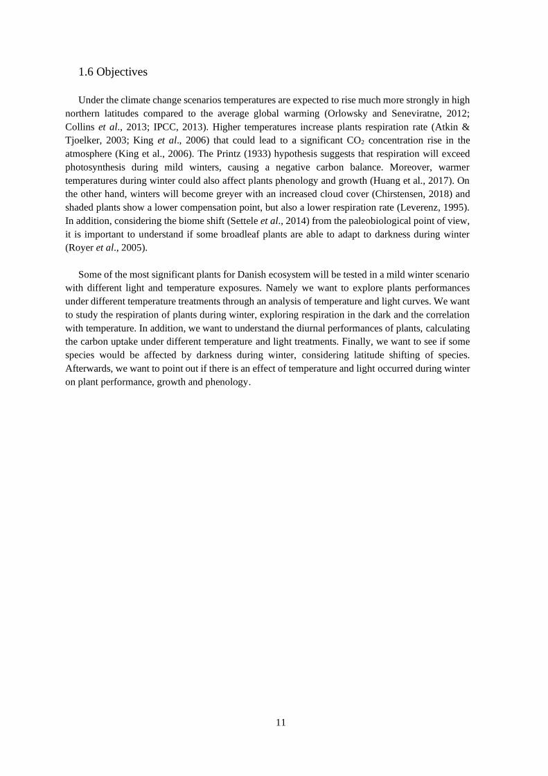
Some of the most significant plants for Danish ecosystem will be tested in a mild winter scenario
with different light and temperature exposures. Namely we want to explore plants performances
under different temperature treatments through an analysis of temperature and light curves. We want
to study the respiration of plants during winter, exploring respiration in the dark and the correlation
with temperature. In addition, we want to understand the diurnal performances of plants, calculating
the carbon uptake under different temperature and light treatments. Finally, we want to see if some
species would be affected by darkness during winter, considering latitude shifting of species.
Afterwards, we want to point out if there is an effect of temperature and light occurred during winter
on plant performance, growth and phenology.

12
2. Materials and Methods
2.1 Plant material
488 seedlings were used for the experiments: 76 Abies alba, 100 Fagus sylvatica, 97 Larix X
eurolepis, 116 Picea abies and 99 Quercus robus. Plants were firstly potted in 20 cm diameter pots, and
then repotted in a 35 cm diameter pot before the growing season, on March 2020. During potting and
repotting two Osmocote fertilizer tabs were added to each pot. Selected plants had different ages and
grew in different ways. At the moment of first potting in August 2019, Abies alba was four years old
and transplanted bare-rooted, Picea abies was one and half years old grown in Jiffy, Larix X eurolepis
was one year old grown in Jiffy, Quercus robur was two years old transplanted bare-rooted, and F.
sylvatica was three years old and already potted (it was previously used for autumn temperatures
experiment in 2018, information about the previous treatment are trackable). Plants origin was also
tracked: Abies alba – FP242 Denmark, Picea abies – FP635 Denmark, Larix X eurolepis – FP203
Denmark, Quercus robur – Elsendrop, Netherlands, and Fagus sylvatica – FP849 Denmark. Seedlings
were placed in outdoor ambient conditions from November 2019 until January 2020. After an initial
screening, removing unhealthy plants, plants were selected and moved to the plots on 3rd of January.
Selection was done by dividing all the species in two groups of taller and shorter plants. After that, two
of each group were selected randomly and moved to an arbitrary plot.
2.2 Experimental designs
The experiments took place in the Arboretum, Horsholm (55°51'57.36"N - 12°30'30.64"E). Plants
were subjected to different light and temperature treatments for one month, from the 7 th of January until
the 7th of February 2020. Outdoor and indoor plots were set respectively in a 500 m2 yard and in four
greenhouses nearby the yard [Fig. 2.1]. The outdoor experimental design ensured that the natural winter
environmental conditions (e.g. humidity, precipitation and wind) were not altered for both control and
heated plots, but the temperature treatment was then limited by heaters capacity in a such cold
environment and with limited energy costs. On the other hand, the indoor treatments didn’t keep the
natural ambient conditions (plants were not subjected to wind and precipitations), but temperature
treatments could be more effective, generating a major gap between control and indoor plots. Therefore,
two different experimental designs were set up for outdoor and indoor experiments, following space and
plants availability. Plants located in the outdoor plots had shoots of the first whorl set at the same
distance (approximately 80 cm) from the heaters to receive an equal amount of heat. Heaters were turned
on during the morning of 7th of January, date that establish the beginning of experimental month of light
and temperature treatment. The treatment ended on the 7th of February. Afterwards, all the plants were
moved to two squared plots and placed in random position in the colder greenhouse (indoor seedlings)
and outside (outdoor seedlings).
2.2.1 Outdoor experiment
Two different temperatures and two different light treatments were designed for this experiment.
Eight 12 m2 hexagonal plots were placed in the yard [Fig. 2.2]. Four plots were heated through six
infrared non-glowing heaters each set at two meters height from the ground, to heat up the canopy inside
the plots, aiming to obtain the highest temperature (+4°C compared to the control plots) at 80 cm from
the ground. Four plots functioned as control with natural environmental conditions, thus six coloured
wooden boards were mounted in each plot, simulating the heaters. In addition, each plot was subjected

13
to two different light exposures. Hence, half of the plants in each plot were covered by a net that
traps 60% of light, and the other half was exposed to ambient light. Nets were fixed on a wooden
structure built inside each plot. The structure was keeping the net between the plants and the heaters.
Plots were named with numbers, from ‘1’ to ‘8’, pair numbers represented heated plots and odd
numbers the control ones. Light treatments were named ‘Light’ to refer to ambient light, and ‘Shade’
to refer to shaded plants. In this way, four different treatments were included: 1) ambient temperature
and ambient light, 2) ambient temperature and shaded, 3) heated and ambient light, and 4) heated
and shaded [Fig. 2.3]. Forty plants were placed in each plot with 20 of them exposed to ambient light
and 20 set in shadow. In particular, seedlings were divided in each plot as follows: 6 Abies alba, 8
Fagus sylvatica, 8 Larix X eurolepis, 10 Picea abies and 8 Quercus robur. Therefore, there were 12
Abies alba, 16 Fagus sylvatica, 16 Larix X eurolepis, 20 Picea abies and 16 Quercus robur per
treatment, resulting in 80 seedlings per treatment and 320 plants in total. The seedlings set in the
plots were surrounded by side plants to limit the wind action and to reach a higher temperature.
Figure 2.1 – Arboretum map. The Arboretum is located at Horsholm (55°51'57.36"N - 12°30'30.64"E). On the top left
the yard used to set up the plots for the outdoor experiment. Greenhouses are evidenced with different colours the evidence
temperature treatments.
2.2.2 Indoor experiment
The indoor experiment was established in 4 greenhouses and a control plot outside. Temperatures
in greenhouses were adjusted by heaters and had different mean temperatures: the warmest (G13)
was 13°C, the warm (G11) was 10.6 °C, the medium (G9) was 8.7 °C, the lowest (G6) was 5.8 °C
and the outside plot 1 had ambient temperature [Fig. 2.4]. Half of the plants were exposed to ambient
light and half to a dark treatment (PAR = 0 µmol m-2 s-1). The latter was realized with a black plastic
cover placed all around the seedlings. Indoor treatments were called ‘Dark’ for plants set in darkness
and ‘Light’ for plant exposed to normal light. 38 or 39 seedlings were placed in each greenhouse
plot, and 13 in darkness outside (plot 1 outdoor was used as ambient light control for this experiment).
The number of seedlings in the greenhouses were divided as follows: 38 plants in G13 and G11, 39
plants in G9 and G6, and 13 plants in dark control outdoor [Tab. 2.1]
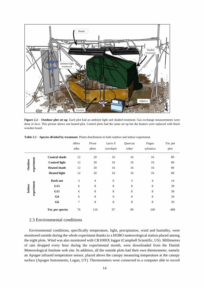
14
Figure 2.2 – Outdoor plot set up. Each plot had an ambient light and shaded treatment. Gas exchange measurements were
done in loco. This picture shows one heated plot. Control plots had the same set up but the heaters were replaced with black
wooden board.
Table 2.1 – Species divided by treatment. Plants distribution in both outdoor and indoor experiment.
2.3 Environmental conditions
Environmental conditions, specifically temperature, light, precipitation, wind and humidity, were
monitored outside during the whole experiment thanks to a HOBO meteorological station placed among
the eight plots. Wind was also monitored with CR1000X logger (Campbell Scientific, US). Millimetres
of rain dropped every hour during the experimental month, were downloaded from the Danish
Meteorological Institute web site. In addition, all the outside plots had their own thermometer, namely
an Apogee infrared temperature sensor, placed above the canopy measuring temperature at the canopy
surface (Apogee Instruments, Logan, UT). Thermometers were connected to a computer able to record
Abies
alba
Picea
abies
Larix X
eurolepis
Quercus
robur
Fagus
sylvatica
Tot. per
plot
Ou
tdo
or
exp
erim
ent Control shade 12 20 16 16 16 80
Control light 12 20 16 16 16 80
Heated shade 12 20 16 16 16 80
Heated light 12 20 16 16 16 80
Ind
oo
r
exp
erim
ent Dark out 3 4 0 3 4 14
G13 6 8 8 8 8 38
G11 6 8 8 8 8 38
G9 6 8 9 8 8 39
G6 7 8 8 8 8 39
Tot. per species 76 116 97 99 100 488
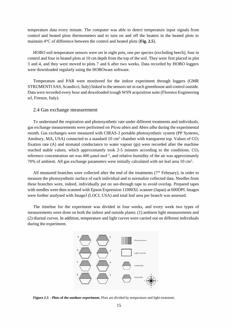
15
temperature data every minute. The computer was able to detect temperature input signals from
control and heated plots thermometers and to turn on and off the heaters in the heated plots to
maintain 4°C of difference between the control and heated plots [Fig. 2.5].
HOBO soil temperature sensors were set in eight pots, one per species (excluding beech), four in
control and four in heated plots at 10 cm depth from the top of the soil. They were first placed in plot
3 and 4, and they were moved to plots 7 and 6 after two weeks. Data recorded by HOBO loggers
were downloaded regularly using the HOBOware software.
Temperature and PAR were monitored for the indoor experiment through loggers (GMR
STRUMENTI SAS, Scandicci, Italy) linked to the sensors set in each greenhouse and control outside.
Data were recorded every hour and downloaded trough WSN acquisition suite (Florence Engineering
srl, Firenze, Italy).
2.4 Gas exchange measurement
To understand the respiration and photosynthetic rate under different treatments and individuals,
gas exchange measurements were performed on Picea abies and Abies alba during the experimental
month. Gas exchanges were measured with CIRAS-3 portable photosynthetic system (PP Systems,
Amsbury, MA, USA) connected to a standard 10 cm2 chamber with transparent top. Values of CO2
fixation rate (A) and stomatal conductance to water vapour (gs) were recorded after the machine
reached stable values, which approximately took 2-5 minutes according to the conditions. CO2
reference concentration set was 400 μmol mol–1, and relative humidity of the air was approximately
70% of ambient. All gas exchange parameters were initially calculated with set leaf area 10 cm2.
All measured branches were collected after the end of the treatments (7 th February), in order to
measure the photosynthetic surface of each individual and to normalize collected data. Needles from
these branches were, indeed, individually put on see-through tape to avoid overlap. Prepared tapes
with needles were then scanned with Epson Expression 11000XL scanner (Japan) at 600DPI. Images
were further analysed with ImageJ (LOCI, USA) and total leaf area per branch was assessed.
The timeline for the experiment was divided in four weeks, and every week two types of
measurements were done on both the indoor and outside plants: (1) ambient light measurements and
(2) diurnal curves. In addition, temperature and light curves were carried out on different individuals
during the experiment.
Figure 2.3 – Plots of the outdoor experiment. Plots are divided by temperature and light treatment.

16
Figure 2.4 – Indoor plot set up. Indoor plots were placed in the four greenhouses setting up a total dark and an ambient light
treatment. Gas exchanges were measured in loco.
Figure 2.5 – Temperature control mechanism for heated and control plots – outdoor experiment. Apogee infrared
sensors in the control plot (top left) and in the heated plot (top right) send two temperature signals, respectively Tc and TH, to
the central computer (down centre). The central computer calculates the difference between TH and TC. If the difference is
less than +4°C the computer sends an output signals that turns on the heaters in the heated plot. In opposite case, the
computer sends a signal that turns them off.

17
2.4.1 Ambient light
Ambient light measurements were done once a week for four weeks. All the plants in each plot
were measured one time under ambient conditions. Data were recorded with different PAR, so that
a wide spectrum of performance under different conditions was obtained [Fig. 2.6].
Figure 2.6 – Gas exchange measurements. They were performed with CIRAS-3 portable photosynthetic system (PP Systems,
Amsbury, MA, USA). On the left a measurement performed with using PLC3 Universal LED Light Unit (RGBW) (PP Systems,
Amsbury, MA, USA), on the right some preliminary tests with the machine using ambient light.
2.4.2 Diurnal curves
Diurnal curves were carried out once a week for four weeks on both indoor and outdoor plots.
Diurnal curves consisted in five cycles of measurements with an approximative range of two hours
each. Measurements were starting before the sunrise and ending after the sunset, in order to measure
both respiration and net photosynthesis. One individual per plot per treatment was randomly selected
during the first cycle and measured during the whole day [Tab. 2.2]. Selected individuals were
changed every week, in order to have data from as many individuals as possible. In addition, the
order in which plots were measured was changing every week (e.g. cycle measurements started at
6:00 am from plot 1 on the first week, and from plot 8 on the second week). Every individual was
measured in loco. Both sunny and cloudy days were chosen to have different levels of PAR and
temperature during the cycles. Daylight was approximately between 7-8 hours from the beginning to
the end of the experimental month. Hence, sunrise was approximately after 8:00, and sunset after
16:00, so that the first and the fifth cycle of measurement were taken in almost darkness.
Table 2.2 – Time scheduled for diurnal curves cycles. Table shows the five cycles of measurements performed during the
day, the first and the last cycle were performed in darkness.
Cycle Time
1 06:00 – 08:00
2 09:30 – 11:30
3 12:00 – 14:00
4 14:30 – 16:00
5 16:30 – 18:30

18
2.4.3 Temperature curves
Temperature curves were performed on Picea abies and Abies alba indoor. Different PAR levels
were obtained thanks to PLC3 Universal LED Light Unit (RGBW) (PP Systems, Amsbury, MA, USA).
Measurements were carried out in the warmest and coldest greenhouses (G13 and G6), testing the plants
at a constant PAR of 100 µmol m-2 s-1 and 200 µmol m-2 s-1. Levels of PAR with which temperature
curves were performed were chosen according to the mean level of light that occurs during winter in
Denmark. Temperature was varied from 3-4°C to 25°C in five steps [Tab. 2.3].
2.4.4 Light curves
Light curves were performed in the four greenhouses on plants exposed to ambient light. Two
individuals per greenhouse per species were randomly chosen among Picea abies and Abies alba.
Curves were obtained using PLC3 Universal LED Light Unit (RGBW) (PP Systems, Amsbury, MA,
USA), that allows to change the amount of light in the leaf chamber. PAR levels were increased from 0
µmol m-2 s-1 to 1000 µmol m-2 s-1. Temperature was set at the ambient temperature of the analysed
greenhouse [Tab. 2.3].
2.5 Plants dimension measurement
Seedlings dimensions, diameter and height, were measured before the 7 th of January and after the
16th of June, therefore before the experimental month and after the full development of new leaves. A
ruler was used to quantify the height of the trunk and a caliber was used to measure the diameter at 8
cm from the ground. This point was marked in order to perform further measurements in the same
position.
Table 2.3 – PAR and temperature levels set for temperature and light curves in different greenhouses. Table shows
number of selected individuals for light and temperature curves, with light and temperature settings we used for each one.
Individuals and greenhouses Set PARs Set Temperatures
Temperature
curves
1 per species per greenhouse
(G13 – G6)
(no dark treatment plants were used)
(100, 200) µmol m-2 s-1 (3, 12, 15, 19, 25) °C
Light curves
2 per species per greenhouse
(G13-G11-G9-G6)
(no dark treatment plants were used)
(0, 20, 40, 60, 80, 100, 150,
200, 500, 1000) µmol m-2 s-1
G13 = 14°C
G11-G9 = 10°C
G6 = 5°C
2.6 Phenology
The phenological development of plants was assessed during the growing season. Since some of the
buds were showing a green colour already during the treatment, data were collected from 3rd of February
[Fig. 2.7]. The monitoring continued with a frequency of one campaign every second week until the
growing season started. It took place once a week since then. Phenology was monitored for all the 488
plants. Buds were evaluated using two different scales, one referred to angiosperms and the other to
conifers [Tab. 2.4]. A score was given to the buds according to the appearance of the majority of the
buds on the up-quarter part of the seedling but excluding the buds at the top of the shoot.
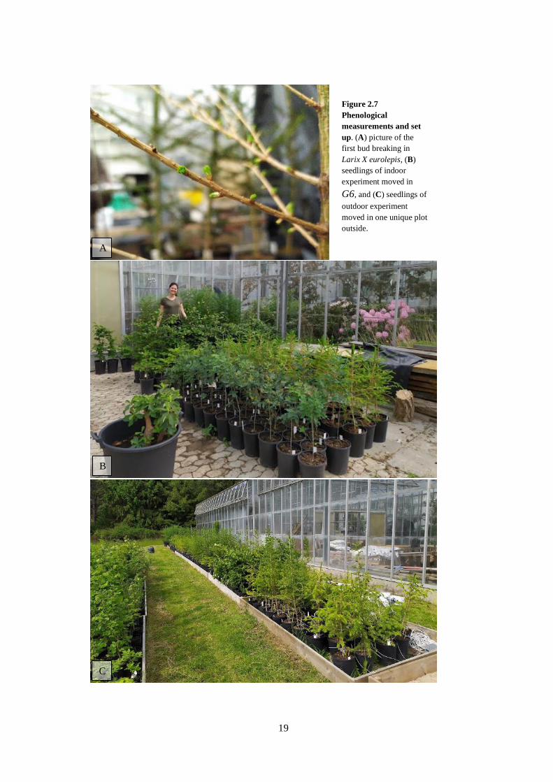
19
A
B
C
Figure 2.7
Phenological
measurements and set
up. (A) picture of the
first bud breaking in
Larix X eurolepis, (B)
seedlings of indoor
experiment moved in
G6, and (C) seedlings of
outdoor experiment
moved in one unique plot
outside.

20
Table 2.4 – Phenological scores for Angiosperms and conifers. Table shows the scores that were given to angiosperms on
the left and scores used to evaluate conifers phenology on the right.
2.7 Statistical Methods
All analyses were performed in R studio and Microsoft Excel 2010.
2.7.1 Meteorological data
Daily average, minimum and maximum temperature was calculated and plotted for each sensor for
the indoor experiment. Mean values of temperature were also calculated within heated and control plots
for the outdoor experiment. In this way, the average, the average minimum and the average maximum
of temperature of control and heated treatments were obtained and plotted. Wind speed and relative
humidity were plotted hour by hour. Millimetres of rain dropped every hour were summed within the
day to calculate the daily millimetres of rain. Average, maximum, minimum and standard deviation of
soil temperature was calculated for each of the treatment from the soil sensor data.
2.7.2 Temperature curves
For each analysed individual, temperature curves were fitted with a second degree polynomial, doing
a squared regression. Temperature optimums (Topt) were calculated as maximums of the functions.
Linear mixed-effect models were performed on the temperature curves data to obtain a model of
Angiosperms
Score Stage Score Stage
0 Winter 5 Very small leaves, just escaped from buds
1 Buds swelling 6 Small leaves at the start of expansion
2 Buds green 7 Leaves in an advanced stage of expansion
3 Buds breaking 8 Leaves have reached final size, but still appear
unhardened, spring-like (bright green).
4 Leaves partly out of
buds 9 Fully developed, fully hardened leaves.
Conifers
Score Stage
0 Bud in winter condition
1 Bud slowly starting to swell, no green is seen
2 Bud swollen, some green is seen, but bud scales are still covering bud
3 Bud scales dropped, bud not elongating or only very little
4 Shoot started to elongate, needles brush-like forward pointing (<3cm)
5 Shoot elongating, still soft needles (>3 cm)
6 Shoot fully elongated
7 Needles turning dark green, fully hardened
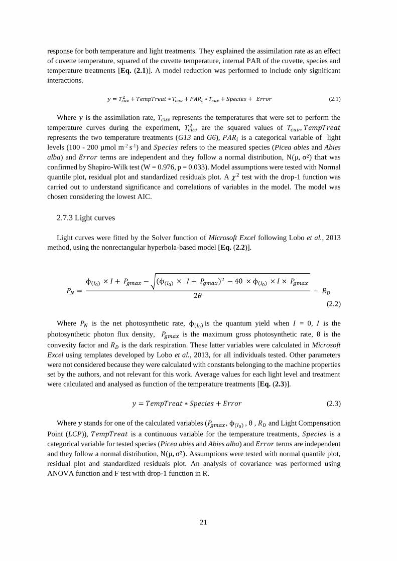
21
response for both temperature and light treatments. They explained the assimilation rate as an effect
of cuvette temperature, squared of the cuvette temperature, internal PAR of the cuvette, species and
temperature treatments [Eq. (2.1)]. A model reduction was performed to include only significant
interactions.
𝑦 = 𝑇𝑐𝑢𝑣2 + 𝑇𝑒𝑚𝑝𝑇𝑟𝑒𝑎𝑡 ∗ 𝑇𝑐𝑢𝑣 + 𝑃𝐴𝑅𝑖 ∗ 𝑇𝑐𝑢𝑣 + 𝑆𝑝𝑒𝑐𝑖𝑒𝑠 + 𝐸𝑟𝑟𝑜𝑟 (2.1)
Where 𝑦 is the assimilation rate, 𝑇𝑐𝑢𝑣 represents the temperatures that were set to perform the
temperature curves during the experiment, 𝑇𝑐𝑢𝑣2 are the squared values of 𝑇𝑐𝑢𝑣, 𝑇𝑒𝑚𝑝𝑇𝑟𝑒𝑎𝑡
represents the two temperature treatments (G13 and G6), 𝑃𝐴𝑅𝑖 is a categorical variable of light
levels (100 - 200 µmol m-2 s-1) and 𝑆𝑝𝑒𝑐𝑖𝑒𝑠 refers to the measured species (Picea abies and Abies
alba) and 𝐸𝑟𝑟𝑜𝑟 terms are independent and they follow a normal distribution, Ν(μ, σ2) that was
confirmed by Shapiro-Wilk test (W = 0.976, p = 0.033). Model assumptions were tested with Normal
quantile plot, residual plot and standardized residuals plot. A 𝜒2 test with the drop-1 function was
carried out to understand significance and correlations of variables in the model. The model was
chosen considering the lowest AIC.
2.7.3 Light curves
Light curves were fitted by the Solver function of Microsoft Excel following Lobo et al., 2013
method, using the nonrectangular hyperbola-based model [Eq. (2.2)].
𝑃𝑁 =
ϕ(𝐼0) × 𝐼 + 𝑃𝑔𝑚𝑎𝑥 − √(ϕ(𝐼0) × 𝐼 + 𝑃𝑔𝑚𝑎𝑥)2 − 4θ × ϕ(𝐼0) × 𝐼 × 𝑃𝑔𝑚𝑎𝑥
2𝜃 − 𝑅𝐷
(2.2)
Where 𝑃𝑁 is the net photosynthetic rate, ϕ(𝐼0) is the quantum yield when 𝐼 = 0, 𝐼 is the
photosynthetic photon flux density, 𝑃𝑔𝑚𝑎𝑥 is the maximum gross photosynthetic rate, θ is the
convexity factor and 𝑅𝐷 is the dark respiration. These latter variables were calculated in Microsoft
Excel using templates developed by Lobo et al., 2013, for all individuals tested. Other parameters
were not considered because they were calculated with constants belonging to the machine properties
set by the authors, and not relevant for this work. Average values for each light level and treatment
were calculated and analysed as function of the temperature treatments [Eq. (2.3)].
𝑦 = 𝑇𝑒𝑚𝑝𝑇𝑟𝑒𝑎𝑡 ∗ 𝑆𝑝𝑒𝑐𝑖𝑒𝑠 + 𝐸𝑟𝑟𝑜𝑟 (2.3)
Where 𝑦 stands for one of the calculated variables (𝑃𝑔𝑚𝑎𝑥 , ϕ(𝐼0) , θ , 𝑅𝐷 and Light Compensation
Point (LCP)), 𝑇𝑒𝑚𝑝𝑇𝑟𝑒𝑎𝑡 is a continuous variable for the temperature treatments, 𝑆𝑝𝑒𝑐𝑖𝑒𝑠 is a
categorical variable for tested species (Picea abies and Abies alba) and 𝐸𝑟𝑟𝑜𝑟 terms are independent
and they follow a normal distribution, Ν(μ, σ2). Assumptions were tested with normal quantile plot,
residual plot and standardized residuals plot. An analysis of covariance was performed using
ANOVA function and F test with drop-1 function in R.
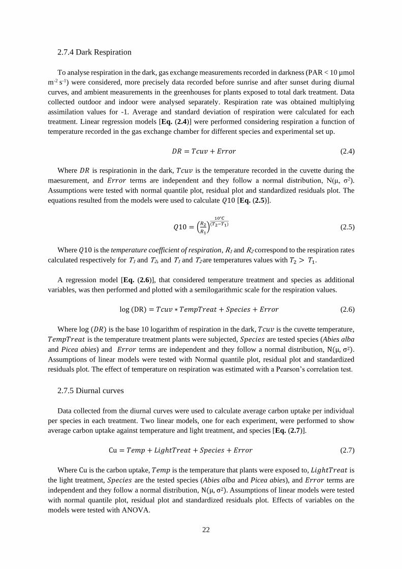
22
2.7.4 Dark Respiration
To analyse respiration in the dark, gas exchange measurements recorded in darkness (PAR < 10 µmol
m-2 s-1) were considered, more precisely data recorded before sunrise and after sunset during diurnal
curves, and ambient measurements in the greenhouses for plants exposed to total dark treatment. Data
collected outdoor and indoor were analysed separately. Respiration rate was obtained multiplying
assimilation values for -1. Average and standard deviation of respiration were calculated for each
treatment. Linear regression models [Eq. (2.4)] were performed considering respiration a function of
temperature recorded in the gas exchange chamber for different species and experimental set up.
𝐷𝑅 = 𝑇𝑐𝑢𝑣 + 𝐸𝑟𝑟𝑜𝑟 (2.4)
Where 𝐷𝑅 is respirationin in the dark, 𝑇𝑐𝑢𝑣 is the temperature recorded in the cuvette during the
maesurement, and 𝐸𝑟𝑟𝑜𝑟 terms are independent and they follow a normal distribution, Ν(μ, σ2).
Assumptions were tested with normal quantile plot, residual plot and standardized residuals plot. The
equations resulted from the models were used to calculate 𝑄10 [Eq. (2.5)].
𝑄10 = (𝑅2
𝑅1)
10°𝐶
(𝑇2−𝑇1) (2.5)
Where 𝑄10 is the temperature coefficient of respiration, R1 and R2 correspond to the respiration rates
calculated respectively for T1 and T2, and T1 and T2 are temperatures values with 𝑇2 > 𝑇1.
A regression model [Eq. (2.6)], that considered temperature treatment and species as additional
variables, was then performed and plotted with a semilogarithmic scale for the respiration values.
log (DR) = 𝑇𝑐𝑢𝑣 ∗ 𝑇𝑒𝑚𝑝𝑇𝑟𝑒𝑎𝑡 + 𝑆𝑝𝑒𝑐𝑖𝑒𝑠 + 𝐸𝑟𝑟𝑜𝑟 (2.6)
Where log (𝐷𝑅) is the base 10 logarithm of respiration in the dark, 𝑇𝑐𝑢𝑣 is the cuvette temperature,
𝑇𝑒𝑚𝑝𝑇𝑟𝑒𝑎𝑡 is the temperature treatment plants were subjected, 𝑆𝑝𝑒𝑐𝑖𝑒𝑠 are tested species (Abies alba
and Picea abies) and 𝐸𝑟𝑟𝑜𝑟 terms are independent and they follow a normal distribution, Ν(μ, σ2).
Assumptions of linear models were tested with Normal quantile plot, residual plot and standardized
residuals plot. The effect of temperature on respiration was estimated with a Pearson’s correlation test.
2.7.5 Diurnal curves
Data collected from the diurnal curves were used to calculate average carbon uptake per individual
per species in each treatment. Two linear models, one for each experiment, were performed to show
average carbon uptake against temperature and light treatment, and species [Eq. (2.7)].
Cu = 𝑇𝑒𝑚𝑝 + 𝐿𝑖𝑔ℎ𝑡𝑇𝑟𝑒𝑎𝑡 + 𝑆𝑝𝑒𝑐𝑖𝑒𝑠 + 𝐸𝑟𝑟𝑜𝑟 (2.7)
Where Cu is the carbon uptake, 𝑇𝑒𝑚𝑝 is the temperature that plants were exposed to, 𝐿𝑖𝑔ℎ𝑡𝑇𝑟𝑒𝑎𝑡 is
the light treatment, 𝑆𝑝𝑒𝑐𝑖𝑒𝑠 are the tested species (Abies alba and Picea abies), and 𝐸𝑟𝑟𝑜𝑟 terms are
independent and they follow a normal distribution, Ν(μ, σ2). Assumptions of linear models were tested
with normal quantile plot, residual plot and standardized residuals plot. Effects of variables on the
models were tested with ANOVA.
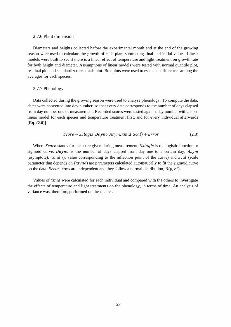
23
2.7.6 Plant dimension
Diameters and heights collected before the experimental month and at the end of the growing
season were used to calculate the growth of each plant subtracting final and initial values. Linear
models were built to see if there is a linear effect of temperature and light treatment on growth rate
for both height and diameter. Assumptions of linear models were tested with normal quantile plot,
residual plot and standardized residuals plot. Box plots were used to evidence differences among the
averages for each species.
2.7.7 Phenology
Data collected during the growing season were used to analyse phenology. To compute the data,
dates were converted into day number, so that every date corresponds to the number of days elapsed
from day number one of measurement. Recorded scores were tested against day number with a non-
linear model for each species and temperature treatment first, and for every individual afterwards
[Eq. (2.8)].
𝑆𝑐𝑜𝑟𝑒 ~ 𝑆𝑆𝑙𝑜𝑔𝑖𝑠(𝐷𝑎𝑦𝑛𝑜, 𝐴𝑠𝑦𝑚, 𝑥𝑚𝑖𝑑, 𝑆𝑐𝑎𝑙) + 𝐸𝑟𝑟𝑜𝑟 (2.8)
Where 𝑆𝑐𝑜𝑟𝑒 stands for the score given during measurement, 𝑆𝑆𝑙𝑜𝑔𝑖𝑠 is the logistic function or
sigmoid curve, 𝐷𝑎𝑦𝑛𝑜 is the number of days elapsed from day one to a certain day, 𝐴𝑠𝑦𝑚
(asymptote), 𝑥𝑚𝑖𝑑 (x value corresponding to the inflection point of the curve) and 𝑆𝑐𝑎𝑙 (scale
parameter that depends on 𝐷𝑎𝑦𝑛𝑜) are parameters calculated automatically to fit the sigmoid curve
on the data. 𝐸𝑟𝑟𝑜𝑟 terms are independent and they follow a normal distribution, Ν(μ, σ2).
Values of 𝑥𝑚𝑖𝑑 were calculated for each individual and compared with the others to investigate
the effects of temperature and light treatments on the phenology, in terms of time. An analysis of
variance was, therefore, performed on these latter.
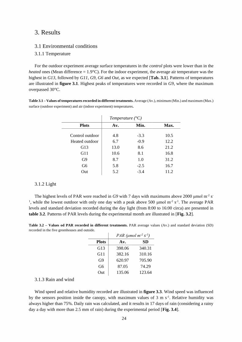
24
3. Results
3.1 Environmental conditions
3.1.1 Temperature
For the outdoor experiment average surface temperatures in the control plots were lower than in the
heated ones (Mean difference = 1.9°C). For the indoor experiment, the average air temperature was the
highest in G13, followed by G11, G9, G6 and Out, as we expected [Tab. 3.1]. Patterns of temperatures
are illustrated in figure 3.1. Highest peaks of temperatures were recorded in G9, where the maximum
overpassed 30°C.
Table 3.1 – Values of temperatures recorded in different treatments. Average (Av.), minimum (Min.) and maximum (Max.)
surface (outdoor experiment) and air (indoor experiment) temperatures.
3.1.2 Light
The highest levels of PAR were reached in G9 with 7 days with maximums above 2000 μmol m-2 s-
1, while the lowest outdoor with only one day with a peak above 500 μmol m-2 s-1. The average PAR
levels and standard deviation recorded during the day light (from 8:00 to 16:00 circa) are presented in
table 3.2. Patterns of PAR levels during the experimental month are illustrated in [Fig. 3.2].
Table 3.2 – Values od PAR recorded in different treatments. PAR average values (Av.) and standard deviation (SD)
recorded in the five greenhouses and outside.
PAR (μmol m-2 s-1)
Plots Av. SD
G13 398.06 340.31
G11 382.16 310.16
G9 620.97 705.90
G6 87.05 74.29
Out 135.06 123.64
3.1.3 Rain and wind
Wind speed and relative humidity recorded are illustrated in figure 3.3. Wind speed was influenced
by the sensors position inside the canopy, with maximum values of 3 m s-1. Relative humidity was
always higher than 75%. Daily rain was calculated, and it results in 17 days of rain (considering a rainy
day a day with more than 2.5 mm of rain) during the experimental period [Fig. 3.4].
Temperature (°C)
Plots Av. Min. Max.
Control outdoor 4.8 -3.3 10.5
Heated outdoor 6.7 -0.9 12.2
G13 13.0 8.6 21.2
G11 10.6 8.1 16.8
G9 8.7 1.0 31.2
G6 5.8 -2.5 16.7
Out 5.2 -3.4 11.2
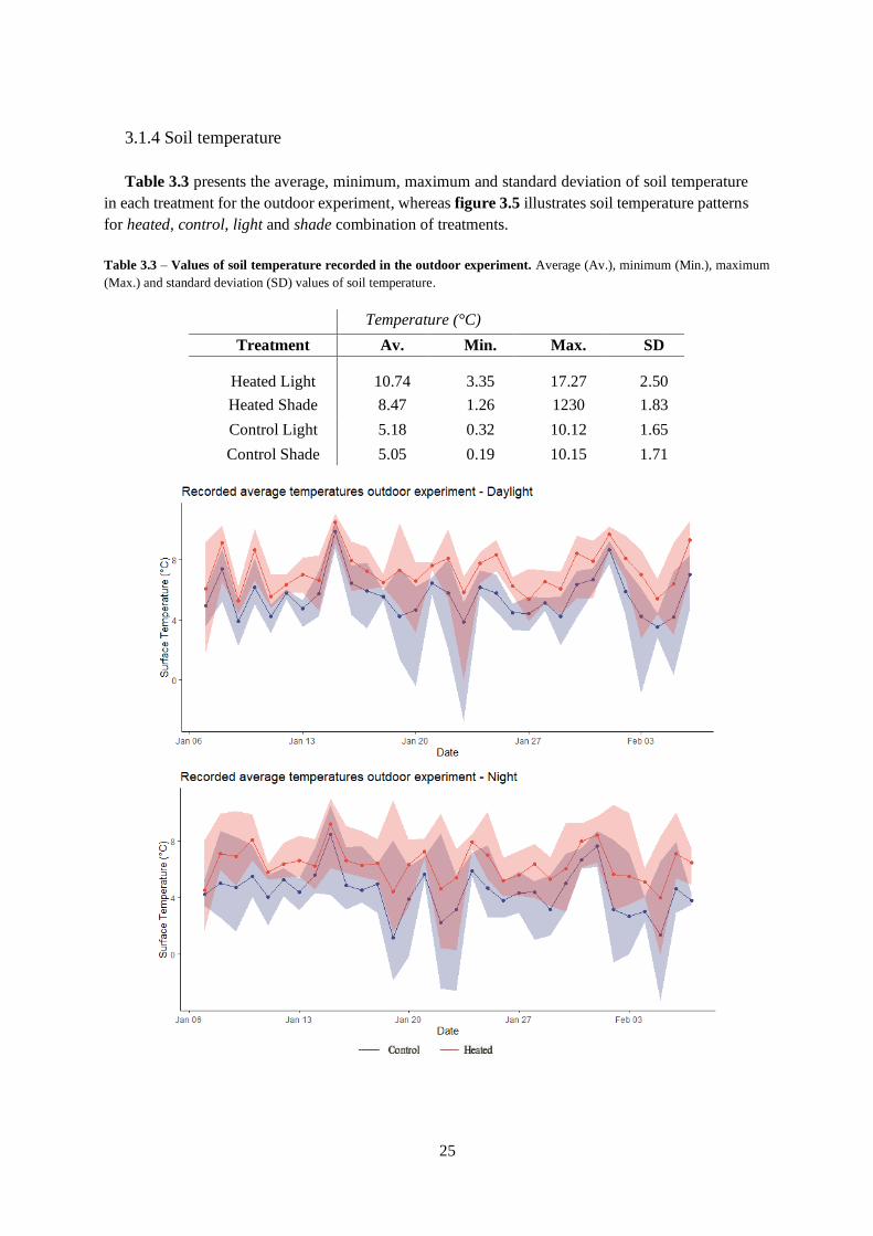
25
3.1.4 Soil temperature
Table 3.3 presents the average, minimum, maximum and standard deviation of soil temperature
in each treatment for the outdoor experiment, whereas figure 3.5 illustrates soil temperature patterns
for heated, control, light and shade combination of treatments.
Table 3.3 – Values of soil temperature recorded in the outdoor experiment. Average (Av.), minimum (Min.), maximum
(Max.) and standard deviation (SD) values of soil temperature.
Temperature (°C)
Treatment Av. Min. Max. SD
Heated Light 10.74 3.35 17.27 2.50
Heated Shade 8.47 1.26 1230 1.83
Control Light 5.18 0.32 10.12 1.65
Control Shade 5.05 0.19 10.15 1.71
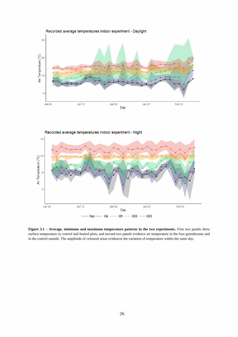
26
Figure 3.1 – Average, minimum and maximum temperature patterns in the two experiments. First two panels show
surface temperature in control and heated plots, and second two panels evidence air temperature in the four greenhouses and
in the control outside. The amplitude of coloured areas evidences the variation of temperature within the same day.
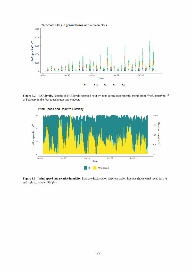
27
Figure 3.2 – PAR levels. Patterns of PAR levels recorded hour by hour during experimental month from 7th of January to 7th
of February in the four greenhouses and outdoor.
Figure 3.3 – Wind speed and relative humidity. Data are displayed on different scales: left axis shows wind speed (m s-1)
and right axis shows RH (%).
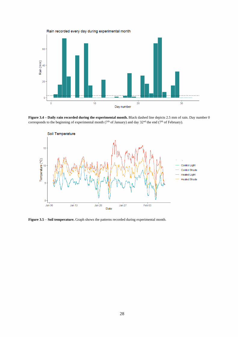
28
Figure 3.4 – Daily rain recorded during the experimental month. Black dashed line depicts 2.5 mm of rain. Day number 0
corresponds to the beginning of experimental month (7th of January) and day 32nd the end (7th of February).
Figure 3.5 – Soil temperature. Graph shows the patterns recorded during experimental month.

29
3.2 Temperature curves
Temperature curves show that the temperature optimum (Topt) varied from a minimum of 3.9° C
(recorded at 100 μmol m-2 s-1 in G13) to a maximum of 22.4°C (recorded at 200 μmol m-2 s-1 in G6)
[Annex I].
Species were not significant in the model (p > 0.05), but the other variables show a significant
effect on the curves [Tab. 3.4]. The curves obtained with the model are illustrated in figure 3.6. It
appears that curves are affected by temperature treatment and light levels, that shifted the assimilation
rate and the Topt. Indeed, assimilation rate was higher for plants subjected to 200 μmol m-2 s-1. The
Topt appeared to be shifted to the right for plants belonging to G6, meaning that plants acclimated to
lower temperatures have a higher optimum of temperature.
Table 3.4 – Effect of the variables in the model with Chi-squared (χ2) test and corresponding p-values. Significance levels
are shown in the following way: 0 ‘***’ 0.001 ‘**’ 0.01 ‘*’ 0.05 ‘.’ 0.1 ‘ ’ 1
Effect Test (𝝌𝟐) p-value
𝑻𝒄𝒖𝒗𝟐 25.6354 4.124e-07 ***
𝑺𝒑𝒆𝒄𝒊𝒆𝒔 1.5991 0.206032
𝑻𝒆𝒎𝒑𝑻𝒓𝒆𝒂𝒕 ∗ 𝑻𝒄𝒖𝒗 4.6213 0.031577 *
𝑷𝑨𝑹𝒊 ∗ 𝑻𝒄𝒖𝒗 9.1377 0.002504 **
Figure 3.6 – Temperature curves fitted with linear mixed-effect model. Light exposition used to perform the curves was
100 μmol m-2 s-1 in the left panel, and 200 μmol m-2 s-1 in the right one. G13 and G6 are the highest and lowest temperature
treatment used in the indoor experiment. Conifers in G13 show lower assimilation than the ones in G6. The graphs also evidence
how the Topt (x axis value corresponding to the maximum of the curve) is slightly higher for plants grown in G6.
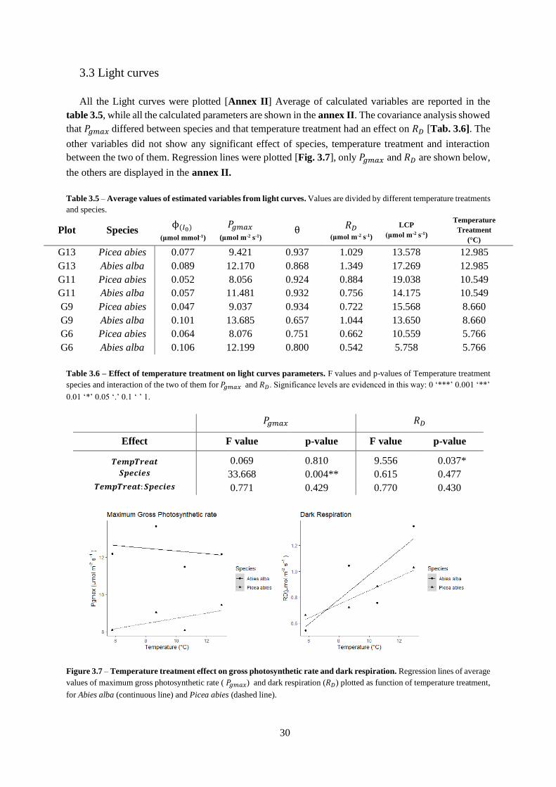
30
3.3 Light curves
All the Light curves were plotted [Annex II] Average of calculated variables are reported in the
table 3.5, while all the calculated parameters are shown in the annex II. The covariance analysis showed
that 𝑃𝑔𝑚𝑎𝑥 differed between species and that temperature treatment had an effect on 𝑅𝐷 [Tab. 3.6]. The
other variables did not show any significant effect of species, temperature treatment and interaction
between the two of them. Regression lines were plotted [Fig. 3.7], only 𝑃𝑔𝑚𝑎𝑥 and 𝑅𝐷 are shown below,
the others are displayed in the annex II.
Table 3.5 – Average values of estimated variables from light curves. Values are divided by different temperature treatments
and species.
Plot Species ϕ(𝐼0)
(μmol mmol-1)
𝑃𝑔𝑚𝑎𝑥
(μmol m-2 s-1) θ
𝑅𝐷
(μmol m-2 s-1)
LCP
(μmol m-2 s-1)
Temperature
Treatment
(°C)
G13 Picea abies 0.077 9.421 0.937 1.029 13.578 12.985
G13 Abies alba 0.089 12.170 0.868 1.349 17.269 12.985
G11 Picea abies 0.052 8.056 0.924 0.884 19.038 10.549
G11 Abies alba 0.057 11.481 0.932 0.756 14.175 10.549
G9 Picea abies 0.047 9.037 0.934 0.722 15.568 8.660
G9 Abies alba 0.101 13.685 0.657 1.044 13.650 8.660
G6 Picea abies 0.064 8.076 0.751 0.662 10.559 5.766
G6 Abies alba 0.106 12.199 0.800 0.542 5.758 5.766
Table 3.6 – Effect of temperature treatment on light curves parameters. F values and p-values of Temperature treatment
species and interaction of the two of them for 𝑃𝑔𝑚𝑎𝑥 and 𝑅𝐷. Significance levels are evidenced in this way: 0 ‘***’ 0.001 ‘**’
0.01 ‘*’ 0.05 ‘.’ 0.1 ‘ ’ 1.
𝑃𝑔𝑚𝑎𝑥 𝑅𝐷
Effect F value p-value F value p-value
𝑻𝒆𝒎𝒑𝑻𝒓𝒆𝒂𝒕 0.069 0.810 9.556 0.037*
𝑺𝒑𝒆𝒄𝒊𝒆𝒔 33.668 0.004** 0.615 0.477
𝑻𝒆𝒎𝒑𝑻𝒓𝒆𝒂𝒕: 𝑺𝒑𝒆𝒄𝒊𝒆𝒔 0.771 0.429 0.770 0.430
Figure 3.7 – Temperature treatment effect on gross photosynthetic rate and dark respiration. Regression lines of average
values of maximum gross photosynthetic rate ( 𝑃𝑔𝑚𝑎𝑥) and dark respiration (𝑅𝐷) plotted as function of temperature treatment,
for Abies alba (continuous line) and Picea abies (dashed line).
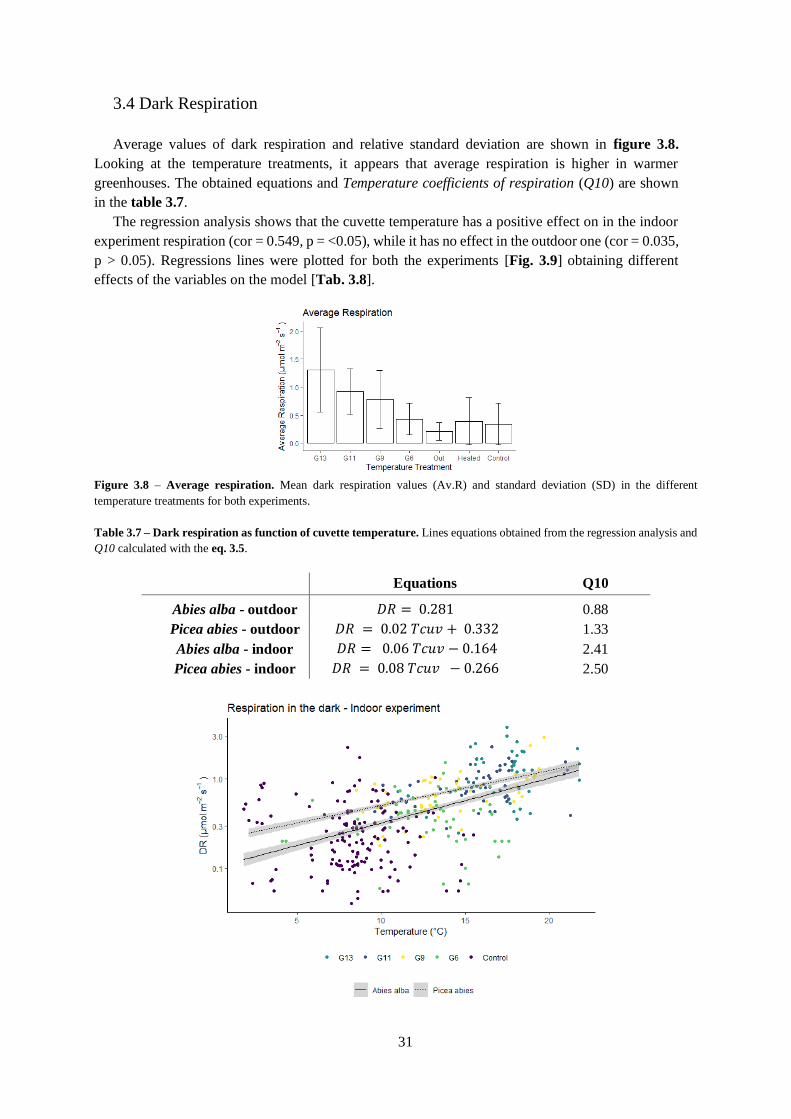
31
3.4 Dark Respiration
Average values of dark respiration and relative standard deviation are shown in figure 3.8.
Looking at the temperature treatments, it appears that average respiration is higher in warmer
greenhouses. The obtained equations and Temperature coefficients of respiration (Q10) are shown
in the table 3.7.
The regression analysis shows that the cuvette temperature has a positive effect on in the indoor
experiment respiration (cor = 0.549, p = <0.05), while it has no effect in the outdoor one (cor = 0.035,
p > 0.05). Regressions lines were plotted for both the experiments [Fig. 3.9] obtaining different
effects of the variables on the model [Tab. 3.8].
Figure 3.8 – Average respiration. Mean dark respiration values (Av.R) and standard deviation (SD) in the different
temperature treatments for both experiments.
Table 3.7 – Dark respiration as function of cuvette temperature. Lines equations obtained from the regression analysis and
Q10 calculated with the eq. 3.5.
Equations Q10
Abies alba - outdoor 𝐷𝑅 = 0.281 0.88
Picea abies - outdoor 𝐷𝑅 = 0.02 𝑇𝑐𝑢𝑣 + 0.332 1.33
Abies alba - indoor 𝐷𝑅 = 0.06 𝑇𝑐𝑢𝑣 − 0.164 2.41
Picea abies - indoor 𝐷𝑅 = 0.08 𝑇𝑐𝑢𝑣 − 0.266 2.50
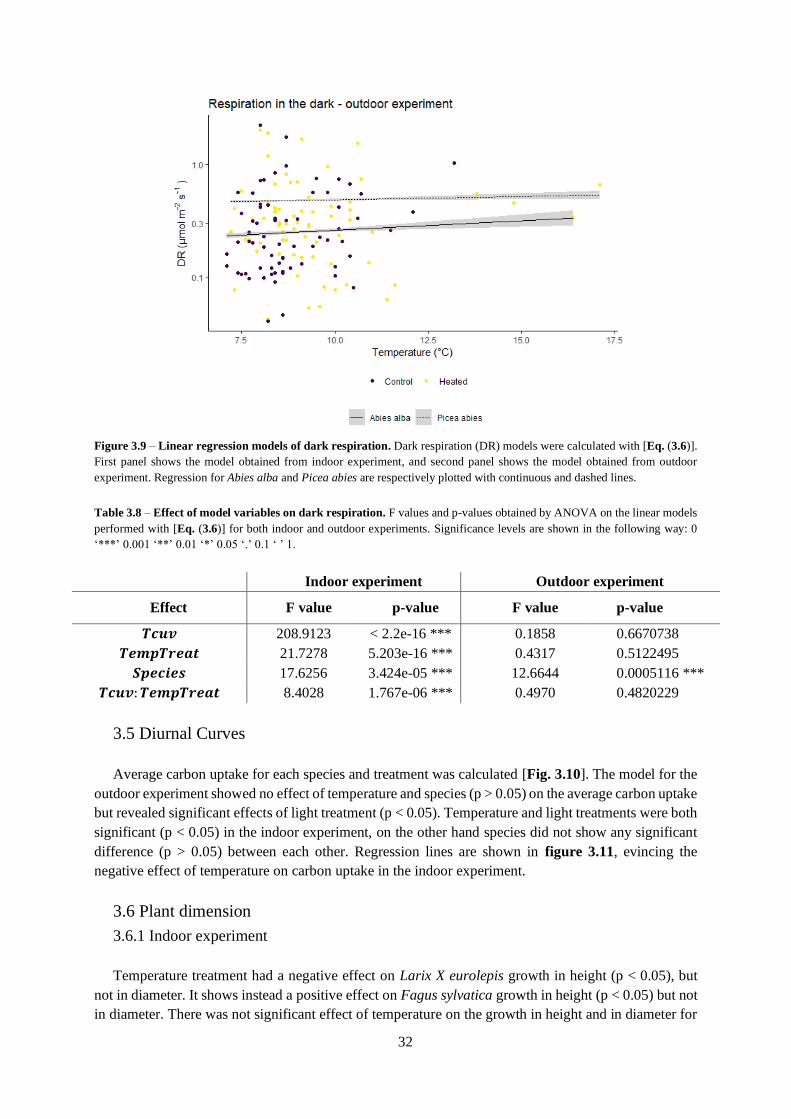
32
Figure 3.9 – Linear regression models of dark respiration. Dark respiration (DR) models were calculated with [Eq. (3.6)].
First panel shows the model obtained from indoor experiment, and second panel shows the model obtained from outdoor
experiment. Regression for Abies alba and Picea abies are respectively plotted with continuous and dashed lines.
Table 3.8 – Effect of model variables on dark respiration. F values and p-values obtained by ANOVA on the linear models
performed with [Eq. (3.6)] for both indoor and outdoor experiments. Significance levels are shown in the following way: 0
‘***’ 0.001 ‘**’ 0.01 ‘*’ 0.05 ‘.’ 0.1 ‘ ’ 1.
Indoor experiment Outdoor experiment
Effect F value p-value F value p-value
𝑻𝒄𝒖𝒗 208.9123 < 2.2e-16 *** 0.1858 0.6670738
𝑻𝒆𝒎𝒑𝑻𝒓𝒆𝒂𝒕 21.7278 5.203e-16 *** 0.4317 0.5122495
𝑺𝒑𝒆𝒄𝒊𝒆𝒔 17.6256 3.424e-05 *** 12.6644 0.0005116 ***
𝑻𝒄𝒖𝒗: 𝑻𝒆𝒎𝒑𝑻𝒓𝒆𝒂𝒕 8.4028 1.767e-06 *** 0.4970 0.4820229
3.5 Diurnal Curves
Average carbon uptake for each species and treatment was calculated [Fig. 3.10]. The model for the
outdoor experiment showed no effect of temperature and species (p > 0.05) on the average carbon uptake
but revealed significant effects of light treatment (p < 0.05). Temperature and light treatments were both
significant (p < 0.05) in the indoor experiment, on the other hand species did not show any significant
difference (p > 0.05) between each other. Regression lines are shown in figure 3.11, evincing the
negative effect of temperature on carbon uptake in the indoor experiment.
3.6 Plant dimension
3.6.1 Indoor experiment
Temperature treatment had a negative effect on Larix X eurolepis growth in height (p < 0.05), but
not in diameter. It shows instead a positive effect on Fagus sylvatica growth in height (p < 0.05) but not
in diameter. There was not significant effect of temperature on the growth in height and in diameter for
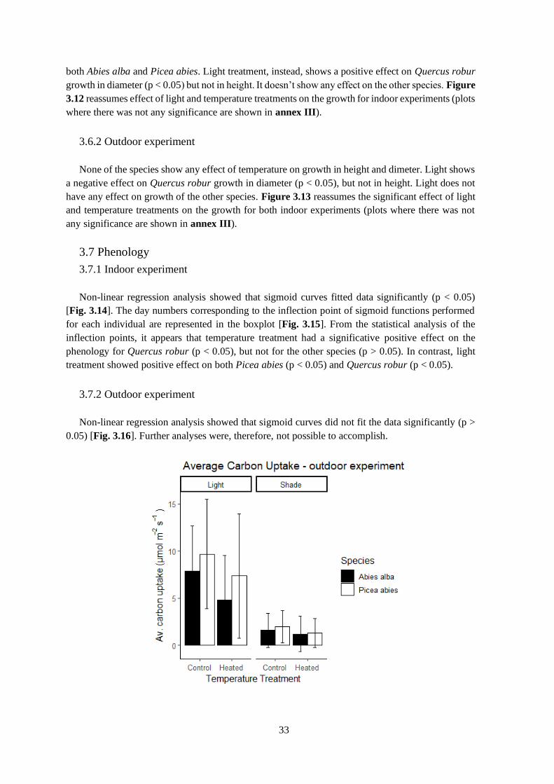
33
both Abies alba and Picea abies. Light treatment, instead, shows a positive effect on Quercus robur
growth in diameter (p < 0.05) but not in height. It doesn’t show any effect on the other species. Figure
3.12 reassumes effect of light and temperature treatments on the growth for indoor experiments (plots
where there was not any significance are shown in annex III).
3.6.2 Outdoor experiment
None of the species show any effect of temperature on growth in height and dimeter. Light shows
a negative effect on Quercus robur growth in diameter (p < 0.05), but not in height. Light does not
have any effect on growth of the other species. Figure 3.13 reassumes the significant effect of light
and temperature treatments on the growth for both indoor experiments (plots where there was not
any significance are shown in annex III).
3.7 Phenology
3.7.1 Indoor experiment
Non-linear regression analysis showed that sigmoid curves fitted data significantly (p < 0.05)
[Fig. 3.14]. The day numbers corresponding to the inflection point of sigmoid functions performed
for each individual are represented in the boxplot [Fig. 3.15]. From the statistical analysis of the
inflection points, it appears that temperature treatment had a significative positive effect on the
phenology for Quercus robur (p < 0.05), but not for the other species (p > 0.05). In contrast, light
treatment showed positive effect on both Picea abies (p < 0.05) and Quercus robur (p < 0.05).
3.7.2 Outdoor experiment
Non-linear regression analysis showed that sigmoid curves did not fit the data significantly (p >
0.05) [Fig. 3.16]. Further analyses were, therefore, not possible to accomplish.

34
Figure 3.10 – Average carbon uptake in the two experiments. Graphs distinguish temperature treatments, light treatments
and species.
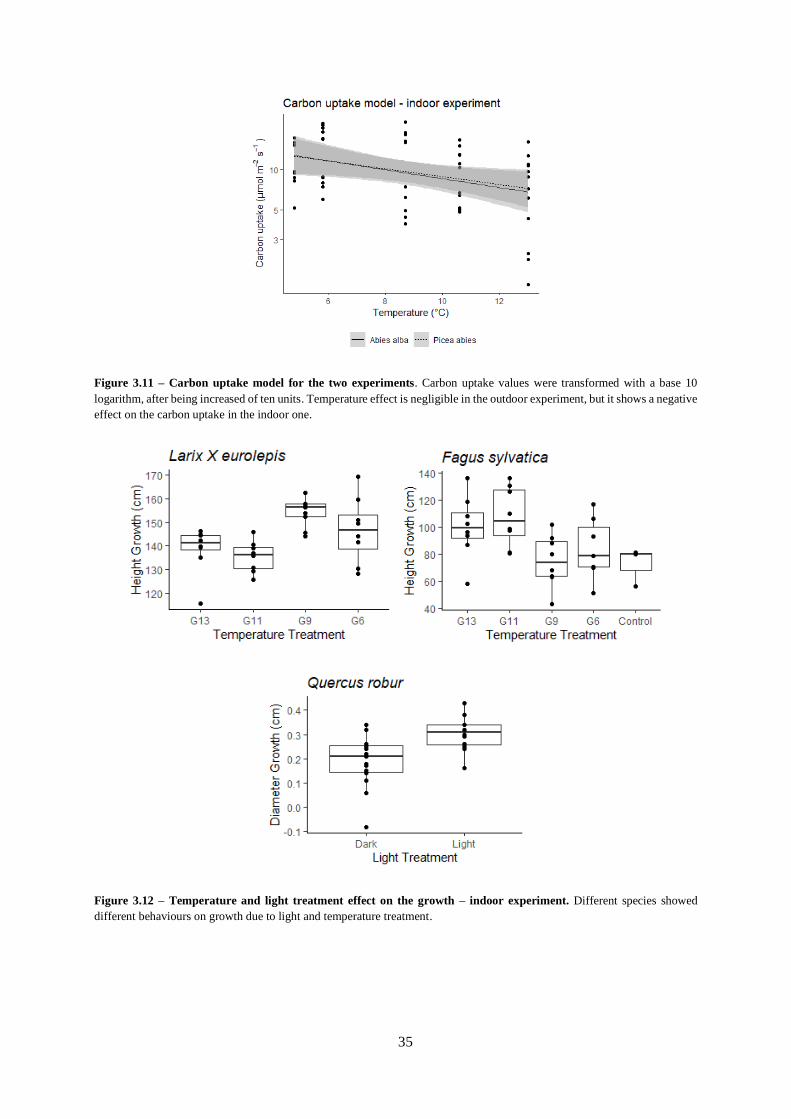
35
Figure 3.11 – Carbon uptake model for the two experiments. Carbon uptake values were transformed with a base 10
logarithm, after being increased of ten units. Temperature effect is negligible in the outdoor experiment, but it shows a negative
effect on the carbon uptake in the indoor one.
Figure 3.12 – Temperature and light treatment effect on the growth – indoor experiment. Different species showed
different behaviours on growth due to light and temperature treatment.
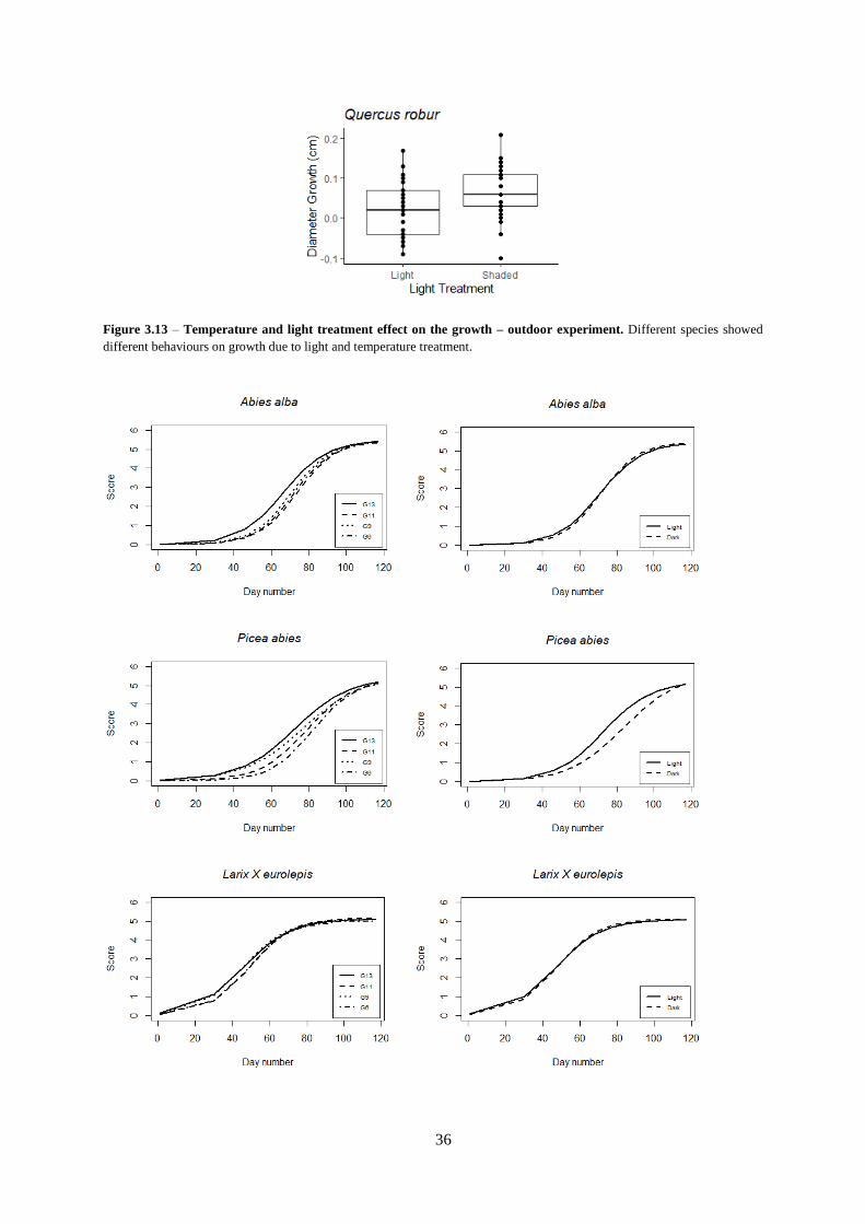
36
Figure 3.13 – Temperature and light treatment effect on the growth – outdoor experiment. Different species showed
different behaviours on growth due to light and temperature treatment.

37
Figure 3.14 – Effect of day number on phenology – indoor experiment. Sigmoid curves explain the effect of day number
on the score for the five analysed species. First five panels distinguish for temperature treatment. In these latter, it is evincible
that the earliest blooming happened for plants belonging to G13. The second six panels differentiate, instead, for light
treatment. Lines overlapped in all the species beside Picea abies, in which plants exposed to light showed an earlier blooming.
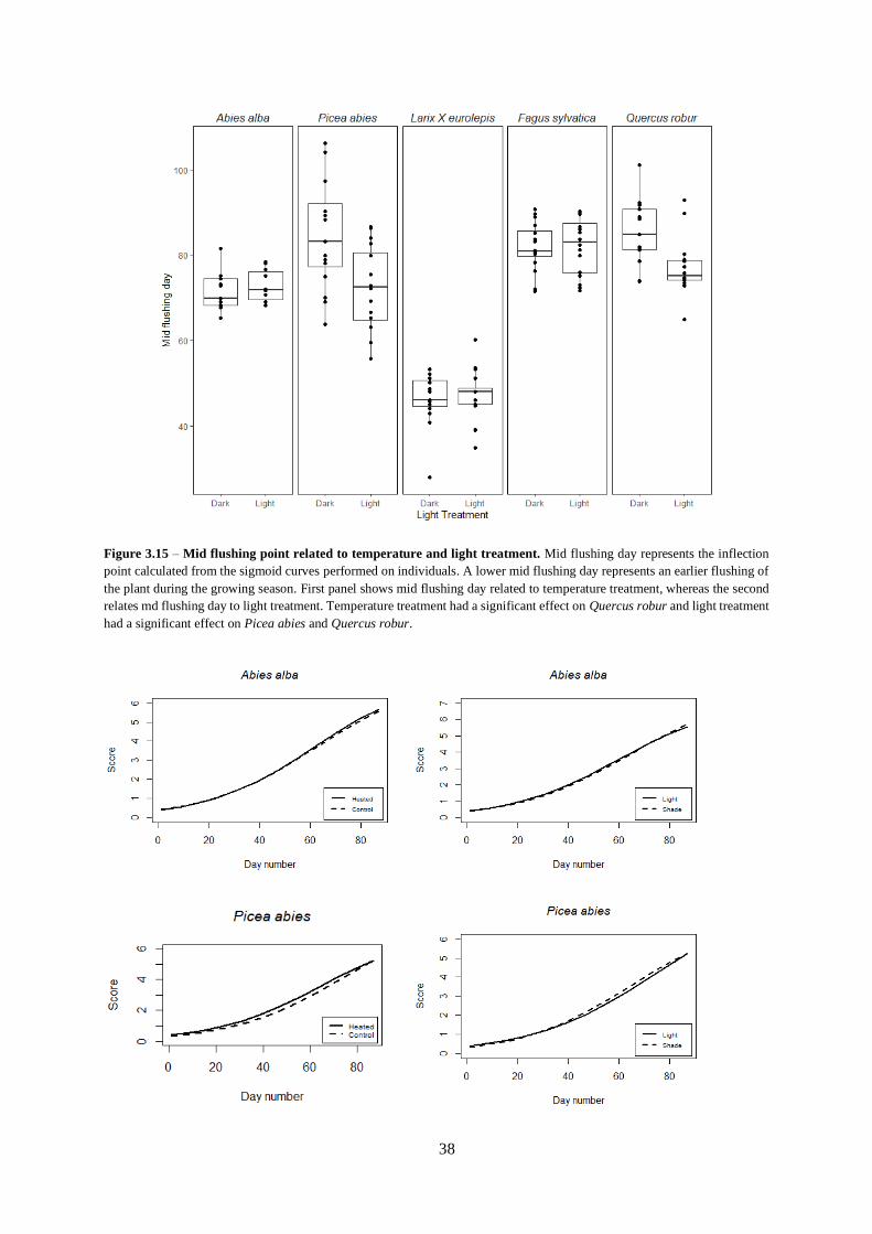
38
Figure 3.15 – Mid flushing point related to temperature and light treatment. Mid flushing day represents the inflection
point calculated from the sigmoid curves performed on individuals. A lower mid flushing day represents an earlier flushing of
the plant during the growing season. First panel shows mid flushing day related to temperature treatment, whereas the second
relates md flushing day to light treatment. Temperature treatment had a significant effect on Quercus robur and light treatment
had a significant effect on Picea abies and Quercus robur.

39
Figure 3.16 – Effect of day number on phenology – outdoor experiment. Sigmoid curves explain the effect of day number
on the score for the five analysed species for outdoor experiment. Left panels differentiate for temperature treatment, instead,
right panels show differences in light treatment.
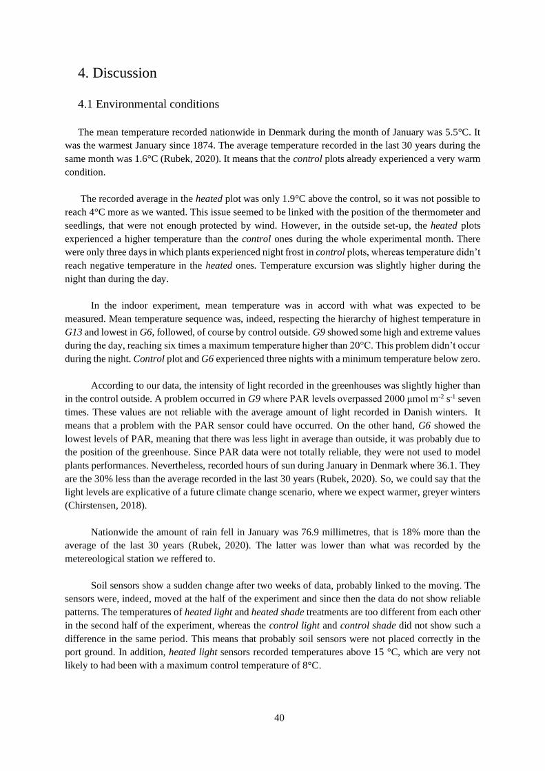
40
4. Discussion
4.1 Environmental conditions
The mean temperature recorded nationwide in Denmark during the month of January was 5.5°C. It
was the warmest January since 1874. The average temperature recorded in the last 30 years during the
same month was 1.6°C (Rubek, 2020). It means that the control plots already experienced a very warm
condition.
The recorded average in the heated plot was only 1.9°C above the control, so it was not possible to
reach 4°C more as we wanted. This issue seemed to be linked with the position of the thermometer and
seedlings, that were not enough protected by wind. However, in the outside set-up, the heated plots
experienced a higher temperature than the control ones during the whole experimental month. There
were only three days in which plants experienced night frost in control plots, whereas temperature didn’t
reach negative temperature in the heated ones. Temperature excursion was slightly higher during the
night than during the day.
In the indoor experiment, mean temperature was in accord with what was expected to be
measured. Mean temperature sequence was, indeed, respecting the hierarchy of highest temperature in
G13 and lowest in G6, followed, of course by control outside. G9 showed some high and extreme values
during the day, reaching six times a maximum temperature higher than 20°C. This problem didn’t occur
during the night. Control plot and G6 experienced three nights with a minimum temperature below zero.
According to our data, the intensity of light recorded in the greenhouses was slightly higher than
in the control outside. A problem occurred in G9 where PAR levels overpassed 2000 μmol m-2 s-1 seven
times. These values are not reliable with the average amount of light recorded in Danish winters. It
means that a problem with the PAR sensor could have occurred. On the other hand, G6 showed the
lowest levels of PAR, meaning that there was less light in average than outside, it was probably due to
the position of the greenhouse. Since PAR data were not totally reliable, they were not used to model
plants performances. Nevertheless, recorded hours of sun during January in Denmark where 36.1. They
are the 30% less than the average recorded in the last 30 years (Rubek, 2020). So, we could say that the
light levels are explicative of a future climate change scenario, where we expect warmer, greyer winters
(Chirstensen, 2018).
Nationwide the amount of rain fell in January was 76.9 millimetres, that is 18% more than the
average of the last 30 years (Rubek, 2020). The latter was lower than what was recorded by the
metereological station we reffered to.
Soil sensors show a sudden change after two weeks of data, probably linked to the moving. The
sensors were, indeed, moved at the half of the experiment and since then the data do not show reliable
patterns. The temperatures of heated light and heated shade treatments are too different from each other
in the second half of the experiment, whereas the control light and control shade did not show such a
difference in the same period. This means that probably soil sensors were not placed correctly in the
port ground. In addition, heated light sensors recorded temperatures above 15 °C, which are very not
likely to had been with a maximum control temperature of 8°C.
41
4.2 Plant performances: temperature and light curves
4.2.1 Temperature curves
The performances of both group of plants were lower in the curves performed at a PAR level of
100 μmol m-2 s-1. Both the assimilation rates increased, indeed, under 200 μmol m-2 s-1 PAR.
Therefore, light was a limiting factor for assimilation, in the first scenario (Perchorowicz et al., 1981;
Dietz and Heber, 1986). Very low levels of light limit the assimilation rate of the conifers.
Nonetheless, the Topt also changed from the two light levels scenarios. In the curves performed with
more light optimums of temperature increased of ≈3°C, for all the plants set respectively in G6 and
G13. The amount of light did not allow the plants to perform at their maximum rates. The choice to
perform temperature curves at such low PAR resemble the typical amount of light that plants could
receive during Danish winters. It is interesting how a very low PAR limits significantly the
assimilation rate. Hence, we must consider the future weather conditions (increasing amount of
clouds) to model photosynthetic data.
Looking at the temperature treatments, it appears that plants acclimated to lower temperatures
had the best performance. Hence, the assimilation rate was higher for those belonging to G6. Since
the species were not significantly different from each other, it means that both Picea abies and Abies
alba perform better if exposed to lower temperatures. It seems, indeed, that they didn’t really
acclimate to such a warm condition (13°C) in G13. They could show a detractive adjustment
behaviour, namely a reduction of assimilation rate if the plants are exposed to warmer temperature.
Not all the species are, in fact, able to acclimate to warmer temperatures in the same way. Evergreen
trees do not very likely adjust their performances to the growth temperature (Wan and Yamori, 2013).
The assimilation rate could also be limited by the amount of photorespiration. Since dark and light
respiration increases with temperature, seedlings that grow at a higher temperature have a higher
respiration rate that results in a lower net assimilation rate (Wan and Yamori, 2013).
Topt also differs between the two temperature treatments at both light levels. The Topt of G13 plants
was ≈5°C lower than Topt of G6 plants. The same difference is conserved in the 200 μmol m-2 s-1 PAR
temperature curves. Meaning that conifers that grew at lower temperatures show a higher Topt. This
look like a contradiction, but if we analysed the matter in the same context, we analysed previous
parameters, it is likely to observe this behaviour. On one hand, a low acclimation of plants to higher
temperature, diminished the performances of the latter under warmer conditions. So, seedlings were
not able to modify their performances to enhance assimilation under different temperature conditions
(Wan and Yamori, 2013). On the other hand, respiration rate increased with temperature lowering
the performance of the plants (Atkin and Tjoelker, 2003, Wan and Yamori, 2013).
These consequences support the idea that photorespiration acclimates faster to temperature than
assimilation does (Wan and Yamori, 2013). This is can be linked with the carboxylation and
oxygenation rate of Rubisco. If we consider that the carboxylation rate increases faster than the
oxygenation at increasing temperatures (Farquhar et al., 1980), it is likely to observe an increasing
of respiration at higher growth temperatures and not a rise of photosynthetic rate. Therefore, the risk
of respiration increasing quicker than fixation could lead to a negative carbon balance at warmer
temperatures.
42
4.2.2 Light curves
Most of the calculated parameters did not show any difference among species or temperature
treatment. Nevertheless, Pgmax and RD show interesting patterns. First, Pgmax was different between the
two species. Abies alba had a higher Pgmax than Picea abies, in all the temperature treatment. This
means that the photosynthetic rate at the light saturation point is higher in Abies alba. Differences of
Pgmax are strictly related with the plant ability to acclimate to different environmental conditions (Jurik
et al., 1988; Dreyer et al., 2001). Nevertheless, there was not significant change of the parameter with
temperature treatment. The maximum photosynthetic capacity of the plants could also be related with
species-specific stomata conductance and concentration of abscisic acid (Aasamaa et al., 2002).
On the other hand, RD does not show any difference between the species. The patterns of the lines
are, indeed, only slightly different from each other. Whereas there is a clear effect of temperature on
both. The average respiration rate calculated in each of the treatment, is higher in the higher temperature
treatment. Meaning that the RD is positively related with the growth temperatures (e.g. Atkin and
Tjoelker, 2003, Wan and Yamori, 2013).
4.3 Respiration and carbon uptake
4.3.1 Dark respiration is influenced by temperature and temperature treatment
Average respiration measured in the dark was higher in temperature treatments with warmer
temperatures in both the indoor and outdoor experiment. The lowest mean value recorded in the
greenhouses was one third of the maximum, that was found in G13. Meaning that a variation of 7°C
increases of three times the respiration rate. The difference among the outside plots was not that relevant
as the one found in the greenhouses. But still, a higher mean value of respiration was found in the heated
plots. Although the standard variation was big enough to reverse the results. However, 1.9°C of
temperature more leaded to 15% higher level of respiration. The conditions of the two experiments were
not comparable, so it was not possible to build a model that covered both the very low temperatures and
the highest recorded in the greenhouses.
The equations calculated by the simple model of dark respiration as a function of temperature
measured in the cuvette, without considering the effect of temperature treatments, show the same pattern
of the average values. Namely, they have very small values of slope, meaning that temperature did not
have a significant effect on this experimental set-up. On the other hand, the equations of indoor
experiment show a significant slope revealing an effect of temperature on RD. The equations looked also
different for the two species. Picea abies shows indeed a very small slope, whether Abies alba has zero
slope in the outdoor experiment. Picea abies has a higher slope than Abies alba in the indoor experiment
too, showing the same trend of indoor experiment. It means that in both the experiments, Picea abies
has a faster increasing of respiration with temperature than Abies alba. The Q10 calculated from the
obtained equations follow, of course, the same trend. Q10 of Picea abies in the outdoor experiment is
51% higher than Abies alba. Nevertheless, the difference of Q10 between the two species is not that
marked in the indoor experiment. Picea abies shows a Q10 that is only 3% higher than Abies alba. Q10
seems to increase with temperature, contrarily to what is supported in many studies (e.g. Atkin and
Tjoelker, 2003). More precise measurements are needed to clarify our results.
43
The models obtained from the two experiments show different trends for the indoor and
outdoor experiment. In the first one there is a significant correlation of dark respiration with the
temperature, where once again Picea abies has a higher intercept than Abies alba, but the latter shows
a slightly higher slope. Regression lines resulted from the outdoor experiment do not show any
correlation with temperature, but a significance difference between the species. The intercept of
Picea abies is, once again higher than Abies alba. It means that the respiration in the darkness of the
first one is higher than the latter. The reason why there is a strong correlation with temperature in the
indoor experiment and no correlation in the second is the lack of measurements at higher
temperatures in the second one. The difference between the two treatments is, in fact, very small,
only 1.9°C, and most of the measurements are gathered in the interval 5-10°C. Whereas in the indoor
experiment the range of measurements is wider, from 5°C to more than 20°, with many differences
between the temperature treatments.
We can anyway conclude that dark respiration exponentially increases with the temperature
recorded at the moment of the measurement but also with the growth temperature and with the
interaction of both. Meaning that seedlings which grow under warmer temperatures could show a
higher respiration rate than the ones that grow under cooler temperatures (Tjoelker et al., 1999; Atkin
and Tjoelker, 2003; King et al., 2006; Kurepin et al., 2018).
4.3.2 The effect of temperature on carbon uptake
Carbon uptake calculated from the diurnal curves show an interesting pattern in both the
experiments. In the outdoor experiment, we can suddenly see how the difference is marked between
the light treatments. Seedlings that were subjected to shade treatment have a lower average net
assimilation. If the average carbon uptake was between 5 μmol m-2 s-1 and 10 μmol m-2 s-1 in the
ambient light treatment, it was under 5 μmol m-2 s-1 in the shade one. This means that the 60% less
of light could halve the diurnal carbon uptake. These results are interesting if considering the climate
change scenario in experimental area. Winters will become greyer than before, due to an increasing
of cloud cover (Chirstensen, 2018). A lower amount of light that plants will receive could lead to a
slower carbon uptake in cold months, following what we found in this experiment. On the other hand,
this question should be better analysed, because many studies show that the radiation that spread
through the cloud cover will increase the amount of light received by the plants, resulting in higher
assimilation rate (Young and Smith, 1983; Doughty et al., 2010). Nevertheless, other studies show a
decrease in carbon uptake under cloud cover conditions (Graham et al., 2003; Dahl et al., 2017).
Discrepancies are linked to the amount of light that is diffused or retained by clouds. However, it is
important to estimate whether one or the other effect prevail.
There is a difference in average carbon uptake among temperature treatments in both the
experiments. In the outdoor experiment, plants subjected to ambient light show a larger difference
between the treatments than the ones under shaded conditions. The controls have indeed between 30-
50% higher average of carbon uptake than heated plots in the ambient light treatment, and an
irrelevant difference in the shade one. However, heated plants show a smaller carbon uptake than the
controls. This difference is much more evident in the indoor experiment. In this case, the carbon
uptake recorded in G6 is four times higher than in G13. Recording the biggest jump between G9 and
G11. This means that there could be a negative exponential relation between carbon uptake and
temperature. Despite this we expected that temperature increases the photosynthetic activity, thus the
carbon uptake under warmer conditions (Delpierre et al., 2009). But this can be reversed considering
evergreen plants during mild winters, were photosynthesis is thought to be more negligible (Printz,
44
1933). In this scenario, the carbon uptake reveals a negative correlation with temperature. In addition,
it has been seen by Piao et al., (2008) that an increased carbon uptake happens during growing season,
meaning spring months, and an overall carbon loss under mild autumnal conditions. Hence, temperature
and length of autumnal season could also lead to a carbon loss (Barichivich et al., 2013). Considering
this, the balance could get worse if we include a very low carbon uptake during winters due temperature
rise. Therefore, annual carbon balance should consider the winter carbon uptake too.
As we consider the dark treatment, we could point out that the average carbon uptake was more
negative where the temperature was higher. G13 has a three times higher carbon loss than G6. Since
there is not photosynthesis, we can consider the carbon uptake as an average carbon loss, meaning
average respiration. So, this follows the trends that we observed so far and many studies have been
shown (Tjoelker et al., 1999; Atkin and Tjoelker, 2003; King et al., 2006; Kurepin et al., 2018).
Species also show a difference in carbon uptake. Contrarily from what we have seen so far, Picea
abies shows a higher carbon uptake than Abies alba. This could be linked to the photosynthetic
performances that the plants had during daylight. Nonetheless, in the dark treatment Picea abies shows
a larger carbon loss than Abies alba. It means, that according with previous measurements, Picea abies,
has a larger respiration rate than Abies alba. In addition, the difference in carbon uptake shows that
Picea abies has from 10-50% higher average carbon uptake, it is larger at lower temperatures than
higher. However, the large error does not really make these results trustable.
Linear models obtained from these measurements do not evidence any significance effect of
temperature in the outdoor experiment. The lines have indeed a very little negative slope. However,
Picea abies has a higher intercept than Abies alba, meaning that it has a slightly higher average carbon
uptake. Neither the temperature treatment nor the species are significantly different from each other. On
the other hand, there was a negative trend of the lines in the indoor experiment. The latter shows that
average carbon uptake decreases exponentially with temperature in both the species. It means that the
effect of temperature on carbon uptake is significant. In particular, the effect concerns the temperature
treatments at which seedlings were exposed to. The carbon uptake halved with an increase of 8°C.
Considering that global warming will cause an increase in average of 4.5°C at northern-latitudes
(Hoegh-Guldberg et al., 2018), the carbon uptake decrease could be significative.
Species did not show any significant difference between each other. This supports the idea that the
variation within the two species that was observed among mean values is too wide to discriminate a
significant different behaviour.
In addition, we can point out an increasing variation of responses with an increase of temperature. If
we observe the range of values covered by the measurements at different temperature treatments, it is
appreciable that the variation in G13 is the 80% wider than in G6. This last point could be very
interesting in the climate change scenario. A wider set of responses leads to an increased uncertainty.
Meaning that, the projections could be more difficult to be tracked. If the pattern of responses is not
clear, we could expect very different behaviours that could obstacle and slow down good management
practices. This finding supports the idea that responses to carbon cycle are very uncertain (Settele et al.,
2014).
Summing up, light treatment influenced carbon uptake, showing larger uptake in ambient light
plots. Temperature, instead, had a negative effect on average carbon uptake. None of the treatment
caused an average negative carbon uptake in the plots exposed to a certain amount of lights.

45
Nevertheless, respiration was measured only twice a day, before sunrise and after sunset, this means
that the measurements exclude overnight respiration. The latter could lead to a diurnal negative
carbon balance. This fact addresses to further measurement to assess a more precise diurnal carbon
balance. Finally, plants exposed to darkness follow the expected trend of negative carbon uptake that
becomes more negative with warmer temperatures. Species show a small difference from each other
with higher carbon uptake and carbon loss in Picea abies. We need to point out that average values
had a significant standard deviation, meaning that more measurements are needed to clarify what
was found.
4.4 Growing season: growth and phenology
4.4.1 Plant growth depends on temperature and light treatments in deciduous trees
Some differences in growth were found in plants subjected to different treatments. In the indoor
experiment, where plants had a wider spectrum of temperatures, only Larix X eurolepis and Fagus
sylvatica showed differences of growth related to temperature treatments. However, they have
different responses to the treatments. Temperatures in G13 and G11 negatively influenced the growth
in height of Larix X eurolepis. The latter, had a higher growth in the lower temperature treatments,
meaning G9 and G6. The highest growth was indeed recorded in G9 where the plants increased in
average more than 150 cm. It has been already reported by Huang et al., (2017) that Larix kaempferi
growth will be negatively influenced by climate warming. In addition, a prolonged exposition to
warmer temperatures could cause growth limitation, especially if this is linked with water scarcity
(Kharuk et al., 2019).
Fagus sylvatica appears to take advantage of the temperature instead. The seedlings placed in
G13 and G11 had a higher growth in height than those placed in the other temperature treatments. In
this case, the highest growth was observed in G11, with an average of little more than 100 cm,
nonetheless, average growth of seedlings placed in G13 was 100 cm. The other temperature
treatments have averages closer to 80 cm. We could distinguish responses above and below 11°C,
there is, indeed, a sort of jump between the treatments. Seedlings grew 25% more in treatments above
11°C. There is a connection between the growing season and winter temperatures. They, indeed,
seem to delay the end of the growth under milder conditions (Prislan et al., 2019). As reported by
Signarbieux et al., (2017) plants of Fagus sylvatica that grew in cooler sites had grown 84% less in
volume and 186% higher stem elongation.
Temperature treatments did not have any effect on the growth in height of the other species, and
none in growth in diameter. The outdoor experiments results, instead, do not show any effect of
temperature treatment in growth of both height and diameter.
Light treatments had an effect only on Quercus robur. The latter had different behaviours if
the amount of light received during the experimental month is considered. The seedlings show a
higher growth in diameter if they were subjected to light instead of total dark treatment, in the indoor
experiment. However, they had a lower growth in diameter compared with shaded plants in the
outdoor experiment. In the first place, we can deduce that light influenced growth in diameter.
Secondly, that there is a different response between indoor and outdoor experiment. Quercus robur
is not a shade-tolerant species (Kunstler et al., 2005), meaning that it should show a lower growth
rate in shadow than in light. Full-light exposition should in fact increase the growth rate of Quercus
robur (Valladares et al., 2000). What we observed in our experiment is in contrast with these results.

46
Shaded plants grew three times more than those exposed to ambient light, in the outdoor experiment,
disagreeing what we expected from previous studies. Nevertheless, full-light plants grew 40% more
than those subjected to dark treatment, in the indoor experiment, agreeing, this time, with the quoted
studies. These contrasting findings can be explained by different responses to the shade level, as already
mentioned in Ziegenhagen and Kausch, (1995). Meaning that, Quercus robbur could be advantage by a
low level of shade and disadvantaged by a high level of it. These findings could limit the northern
shifting of Quercus robur, meaning that the absence of light could negatively influence the growth of
this species. In addition, our study refers to differences in light levels during dormancy and not during
growing season, addressing for the necessity of more studies during winter.
All the other plants did not show any effect of light on their growth in both height and diameter. Our
results open a new window on the importance to study the effect of light and temperature treatments on
growth during dormancy. Evergreen trees did not show any effect on growth.
4.4.2 Phenology
There are interesting findings about the phenological responses of plants after one month of light and
temperature treatments. The indoor experiments gave us the chance to study those effects, whereas the
outdoor experiment had too much variation within the measurements to perform significant fits of
sigmoid curves, even excluding some outliers. So, we will not focus on the discussion of those data in
this project.
Data fitted with a sigmoid curve gave homogeneous results for temperature treatments, and different
responses for light treatments. All the species subjected to warmer treatments during winter show an
advancement of phenology. Specifically, seedlings placed in G13 had the highest advancement in
phenology. Evergreen conifers, namely Abies alba and Picea abies show major difference between the
warmest and the other treatments. Whereas, the difference in treatments is not that evident in Larix X
eurolepis. Finally, deciduous broad leaves trees, namely Fagus sylvatica and Quercus robur reveal a
lower difference than evergreen conifers among the treatments. However, all the graphs evidence that
G6 sigmoid is the one that is moved the most to the right, meaning that phenological events of those
plants result delayed compared to the other greenhouses. The order of other curves is not linear, in some
cases plants set in G9 are shifted more to the left than those set in G11.
Our study shows that the temperature treatments at which plants were exposed from January to
February had an effect on the timing of phenological events. Especially, plants exposed to warmer
treatments result in an advancement of phenology. Meaning that winter temperature influences flushing
time (Vitasse et al., 2009). These results show the pattern that we expected to see under warmer
conditions due to climate change, meaning an advancement of phenological events (Kramer, 1995;
Cleland et al., 2007; Penuelas et al., 2009; Vitasse et al., 2009; Körner and Basler, 2010). Contrarily,
more recent studies reveal a different consequence in plant phenology due to warmer winters. Warmer
winters seem, instead, to delay phenological events, due to a lack of chilling temperatures required to
break endodormancy (Körner and Basler, 2010; Signarbieux et al., 2017; Asse et al., 2018). However,
the degree of advancement and delay is species specific. Beech trees had a higher advancement at cooler
conditions. Whether, some species that need lower chilling during winter to stimulate budburst, like
Picea abies, did not evidence a phenological delay, but rather an advancement at warmer temperatures
(Signarbieux et al., 2017; Asse et al., 2018).

47
To better compare the results, it is important to understand the distribution of inflection points
of each individual phenological curve. The inflection point corresponds to approximately half of the
maximum score, meaning the budburst occurrence. We expected to see the same pattern that was shown
by the models that we used to understand the responses of plants divided by treatment. But we found
a greater variety among data, so that only Quercus robur revealed a significant effect of temperature
on the mid flushing day. Therefore, plants exposed to G13 had the most advance budburst, around
the 75th day. Budburst occurred few days later in G11 and G9, whereas it had a delay of 15 days in
G6, where it happened around the 90th day. So, temperature significantly advanced the budburst in
Quercus robur.
The other species don’t have a significant difference related to temperature, but some patterns can
be seen. Differences between the warmest and the coldest greenhouses, namely G13 and G6, are ≈+4
days for Abies alba, ≈+ 14 days for Picea abies, 0 days Larix X eurolepis and ≈+7 days for Fagus
sylvatica. We can deduce that the most affected plants by the temperature treatments, in terms of
phenology advancement, are Quercus robur and Picea abies, although the responses have more
variability in the latter. Our results agree with the fact that the first species is very sensible to
temperature effect (Vitasse et al., 2009) and that the second show a phenological advancement during
warmer winters (Asse et al., 2018). Since responses have similar trends but very different range
between days of advancement and delay, it is important to study species-specific response to
temperatures (Vitasse et al., 2009).
Indoor plants revealed different responses to light treatment in some species. The sigmoid
curves of Picea abies and Quercus robur evidenced discrepancies in day number for certain
phenological events. Whereas, the other species did not show any evidence of light treatment in the
shape and position of the curves. Seedlings of the evergreen conifer exposed to ambient light
treatment flushed earlier than those exposed to full darkness. The same behaviour was observed in
Quercus robur, with a slightly lower difference than Picea abies. These evidences were also
supported by the results found in the comparing of mid flushing day, where plants subjected to total
darkness treatment showed budburst delayed of ≈+ 10 days for Picea abies and ≈+ 9 days for Quercus
robur. These findings are interesting in the context of north pole ward moving of species due to
climate change (Settele et al., 2014). If in the future these species will be able to survive to polar
conditions, there could be mismatches in the phenology of some of them, like Picea abies and
Quercus robur in terms of delay in the budburst, due to the absence of light during winter. On the
other hand, other species could not be affected by darkness, meaning that they could adapt better at
dark and warm conditions (Royer et al., 2005).
Phenology is influenced by winter temperature and winter light exposure. The beginning of
growing season is leaded by daylength, degree of winter chilling and temperature in the days before
the flushing (Vitasse et al., 2009; Körner and Basler, 2010, Visser and Gienapp, 2019). As we have
seen, shift in the phenology is species-specific (Visser and Gienapp, 2019). In addition, it influences
the length of growing season (Penuelas et al., 2010). Warmer winters seem to have a major effect on
autumn phenology than early spring (Suonan et al., 2017), with a consistent legacy between spring
and autumn events, especially at cooler conditions (Signarbieux et al., 2017). Therefore, an earlier
spring can be followed by an earlier autumn senescence, meaning that future models should include
spring phenology events to forecast autumn phenology events (Keenan and Richardson, 2015).
Considering that the advancement of phenological events will be greater at northern latitudes (Liu et
al., 2019), further studies are needed to better model phenological response of species in climate
change scenario.

48
49
5. Conclusion
Temperature and light treatments had an effect on plants performances, growth and phenology.
Major effects were seen in the indoor experiment, where plants could experience a much higher
difference of temperature than in the outdoor one.
Warm winter temperatures negatively affect photosynthesis and respiration. Conifers were not
improving their performances under milder conditions. Net photosynthesis was lower for plants
grown at warmer temperatures, and the temperature optimum was not matching the growth
temperature. It revealed a scarce acclimation of conifers to mild winter temperature. In addition, very
low light level limited photosynthesis. Respiration in the dark showed a correlation with temperature
treatment.
The models evidenced a exponential increasing of respiration in the dark due to growth
temperature and temperature in the moment of measurement. So, we could say that it is important
to consider both the average growth temperature and the daily temperature to understand properly
the trend of respiration in future climate change scenarios. Picea abies and Abies alba had different
level of respiration, a markedly higher respiration was recorded in the first one.
A very small difference between the two species was also seen in the carbon uptake levels in
different treatments. Picea abies enhanced the respiration rate in the dark faster, and it showed a
slightly higher carbon uptake than Abies alba. These differences were flattened in the carbon uptake
model, were no difference between the two species was seen as response of growth temperature.
Carbon uptake was found to decrease exponentially with growth temperature of seedlings,
addressing more studies to understand if respiration is the only cause of this decreasing or if there
are other reasons. In addition, the variation among measurements was also wider with warmer
temperature treatment. Meaning we expect to see a widespread set of responses, making more
difficult future projections under global warming.
Growth in height was influenced by temperature in different ways, namely Larix X eurolepis had
negative effect of high temperatures in winter and Fagus sylvatica was instead advantaged by warmer
winters, both of them showed an effect for the growth in height but not in diameter. On the other
hand, Quercus robur exposed to dark treatment had a lower growth in diameter than ambient light,
despite, it showed an enhanced growth in diameter in the shaded treatment than ambient light. This
species could have very different responses (Morin et al., 2010). Evergreen conifers didn’t show any
significant difference in the growth if subjected to low o light or darkness, or with warmer or cooler
temperatures.
Phenology was contrarily high influenced by winter temperature. All the plants that grew at
warmer temperatures had an advancement in phenology comparing with cooler temperatures. The
number of days was strictly related to the species. However, Quercus robur and Picea abies had the
higher number of days of advancement. In addition, winter darkness seemed to drive certain species
through a delay in spring phenology events, in particular Picea abies and Quercus robur. Phenology
mismatches due to warming winters are very likely to happen. As we have seen not all the species
are affected in the same way by physical conditions (Visser and Gienapp, 2019). Further studies are
needed to understand populations dynamics in forest ecosystem.

50
This study shows that warmer winters have significant effect on winter performances in terms of
carbon uptake and respiration, addressing to more studies needed to calculate carbon balance during
winter months and to assess global scale carbon trend under climate warming. In addition, we have seen
an effect of warmer temperatures on both growth and phenology, showing that it is important to include
winter climate in future modelling to better understand the effect of climate change. Nevertheless, light
had interesting effects on growth and phenology, meaning that it is important to comprehend darkness
tolerance for species that will move pole ward under high latitude warming, especially for long term
forest management and planning.
Not all the species react in the same way to global warming. Those that are weaker and less resilient
need lot of attention under this dramatic scenario. Biodiversity should be preserved and in order to do
that we need to take into account all the multifaced and complex aspects of ecosystems. Therefore, many
efforts are needed to better comprehend this complicated issue that nature has been facing. All the
responses are incredibly important to lead the best decisions for living organisms and ecosystem
survival, and most important, functioning.
51
Bibliography
Aasamaa, K., Sõber, A., Hartung, W., & Niinemets, Ü. (2002). Rate of stomatal opening, shoot
hydraulic conductance and photosynthetic characteristics in relation to leaf abscisic acid
concentration in six temperate deciduous trees. Tree Physiology, 22(4), 267-276.
Anderson-Teixeira, K. J. (2018). Prioritizing biodiversity and carbon. Nature Climate Change,
8(8), 667–668.
Asse, D., Chuine, I., Vitasse, Y., Yoccoz, N. G., Delpierre, N., Badeau, V., ... & Randin, C. F.
(2018). Warmer winters reduce the advance of tree spring phenology induced by warmer springs in
the Alps. Agricultural and Forest Meteorology, 252, 220-230.
Atkin, O. K., & Tjoelker, M. G. (2003). Thermal acclimation and the dynamic response of plant
respiration to temperature. Trends in plant science, 8(7), 343-351.
Barichivich, J., Briffa, K. R., & Myneni, R. B. (2013). Large-scale variations in the vegetation
growing season and annual cycle of atmospheric CO 2 at high northern latitudes from 1950 to 2011.
Global change Biology, 19, 3167–3183.
Bauwe, H., Hagemann, M., Kern, R., & Timm, S. (2012). Photorespiration has a dual origin and
manifold links to central metabolism. Current opinion in plant biology, 15(3), 269-275.
Blankenship, R. E., and Prince, R. C. (1985). Excited-state redox potentials and the Z scheme of
photosynthesis. Trends Biochem. Sci. 10:382-383.
Bourdeau, P. F. (1959). Seasonal variations of the photosynthetic efficiency of evergreen conifers.
Ecology, 40(1), 63-67.
Briceño-Elizondo, E., Garcia-Gonzalo, J., Peltola, H., Matala, J., & Kellomäki, S. (2006).
Sensitivity of growth of Scots pine, Norway spruce and silver birch to climate change and forest
management in boreal conditions. Forest Ecology and Management, 232(1–3), 152–167.
Bukhov, N. G. (2004). Dynamic Light Regulation of Photosynthesis ( A Review ). 51(6), 742–
753.
Cappelen, J. (2020, January 31). Klimaet frem til i dag, https://www.dmi.dk/klima/temaforside-
klimaet-frem-til-i-dag/temperaturen-i-danmark/.
Christensen, O. B. (2018, September 5). Varmere luft kan optage mere vand,
https://www.dmi.dk/klima/temaforside-fremtidens-klima/varmere-luft-kan-optage-mere-vand/.
Chuine, I., & Régnière, J. (2017). Process-Based Models of Phenology for Plants and Animals.
Annual Review of Ecology, Evolution, and Systematics, 48, 159–182.
Cleland, E. E., Chuine, I., Menzel, A., Mooney, H. A., & Schwartz, M. D. (2007). Shifting plant
phenology in response to global change. Trends in Ecology and Evolution, 22(7), 357–365.

52
Cleland, W. W., Andrews, T. J., Gutteridge, S., Hartman, F. C., & Lorimer, G. H. (1998). Mechanism
of rubisco: The carbamate as general base. Chemical Reviews, 98(2), 549–561.
Collins, M., Knutti, R., Arblaster, J., Dufresne, J. L., Fichefet, T., Friedlingstein, P., ... & Shongwe,
M. (2013). Long-term climate change: projections, commitments and irreversibility. In Climate Change
2013-The Physical Science Basis: Contribution of Working Group I to the Fifth Assessment Report of
the Intergovernmental Panel on Climate Change (pp. 1029-1136). Cambridge University Press.
Cooper, E. J. (2014). Warmer shorter winters disrupt Arctic terrestrial ecosystems. Annual Review
of Ecology, Evolution, and Systematics, 45, 271-295.
Dahl, M. B., Priemé, A., Brejnrod, A., Brusvang, P., Lund, M., Nymand, J., ... & Haugwitz, M. S.
(2017). Warming, shading and a moth outbreak reduce tundra carbon sink strength dramatically by
changing plant cover and soil microbial activity. Scientific reports, 7(1), 1-13.
Delpierre, N., Soudani, K., Francois, C., Köstner, B., Pontailler, J. Y., Nikinmaa, E., ... & Grünwald,
T. (2009). Exceptional carbon uptake in European forests during the warm spring of 2007: a data–model
analysis. Global Change Biology, 15(6), 1455-1474.
Dietz, K. J., & Heber, U. (1986). Light and CO2 limitation of photosynthesis and states of the
reactions regenerating ribulose 1, 5-bisphosphate or reducing 3-phosphoglycerate. Biochimica et
Biophysica Acta (BBA)-Bioenergetics, 848(3), 392-401.
Doughty, C. E., Flanner, M. G., & Goulden, M. L. (2010). Effect of smoke on subcanopy shaded
light, canopy temperature, and carbon dioxide uptake in an Amazon rainforest. Global Biogeochemical
Cycles, 24(3).
Dreyer, E., Le Roux, X., Montpied, P., Daudet, F. A., & Masson, F. (2001). Temperature response
of leaf photosynthetic capacity in seedlings from seven temperate tree species. Tree Physiology, 21(4),
223–232.
Dulamsuren, C., Hauck, M., Kopp, G., Ruff, M., & Leuschner, C. (2017). European beech responds
to climate change with growth decline at lower, and growth increase at higher elevations in the center
of its distribution range (SW Germany). Trees, 31(2), 673-686.
Dusenge, M. E., Duarte, A. G., & Way, D. A. (2019). Plant carbon metabolism and climate change:
elevated CO2 and temperature impacts on photosynthesis, photorespiration and respiration. New
Phytologist, 221(1), 32–49.
Environmental Protection Agency. (n.d.). Forestry, https://eng.mst.dk/trade/forestry/
Fahey, T. J., Woodbury, P. B., Battles, J. J., Goodale, C. L., Hamburg, S. P., Ollinger, S. V., &
Woodall, C. W. (2010). Forest carbon storage: Ecology, management, and policy. Frontiers in Ecology
and the Environment, 8(5), 245–252.
FAO and UNEP. 2020. The State of the World’s Forests 2020. Forests, biodiversity and people.
Rome
FAO. 2020. Global Forest Resources Assessment 2020: Main report. Rome.
53
Farquhar, G. D., von Caemmerer, S., & Berry, J. A. (1980). A biochemical model of
photosynthetic CO2 assimilation in leaves of C3 species. Planta, 149(1), 78–90.
Foyer, C. H., Bloom, A. J., Queval, G., & Noctor, G. (2009). Photorespiratory metabolism: Genes,
mutants, energetics, and redox signaling. Annual Review of Plant Biology, 60, 455–484.
Foyer, C. H., Lelandais, M., & Kunert, K. J. (1994). Photooxidative stress in plants. Physiologia
Plantarum, 92(4), 696–717.
FRA. 2020. Global Forest Resources Assessment 2020 report, Denmark. Rome.
Fu, Y. S. H., Campioli, M., Vitasse, Y., De Boeck, H. J., Van Den Berge, J., AbdElgawad, H.,
Asard, H., Piao, S., Deckmyn, G., & Janssens, I. A. (2014). Variation in leaf flushing date influences
autumnal senescence and next year’s flushing date in two temperate tree species. Proceedings of the
National Academy of Sciences of the United States of America, 111(20), 7355–7360.
Gazol, A., Camarero, J. J., Gutiérrez, E., Popa, I., Andreu-Hayles, L., Motta, R., Nola, P., Ribas,
M., Sangüesa-Barreda, G., Urbinati, C., & Carrer, M. (2015). Distinct effects of climate warming on
populations of silver fir (Abies alba) across Europe. Journal of Biogeography, 42(6), 1150–1162.
Geßler, A., Keitel, C., Kreuzwieser, J., Matyssek, R., Seiler, W., & Rennenberg, H. (2007).
Potential risks for European beech (Fagus sylvatica L.) in a changing climate. Trees - Structure and
Function, 21(1), 1–11.
Givnish, T. J. (1988). Adaptation to sun and shade: a whole-plant perspective. Functional Plant
Biology, 15(2), 63-92.
Graham, E. A., Mulkey, S. S., Kitajima, K., Phillips, N. G., & Wright, S. J. (2003). Cloud cover
limits net CO2 uptake and growth of a rainforest tree during tropical rainy seasons. Proceedings of
the National Academy of Sciences, 100(2), 572-576.
Gu, L., Post, W. M., Baldocchi, D., Andy Black, T., Verma, S. B., Vesala, T., & Wofsy, S. C.
(2003). Phenology of Vegetation Photosynthesis. 467–485.
Hadden, D., & Grelle, A. (2016). Changing temperature response of respiration turns boreal forest
from carbon sink into carbon source. Agricultural and Forest Meteorology, 223, 30-38.
Hansen, J. K., & Larsen, J. B. (2004). European silver fir (Abies alba Mill.) provenances from
Calabria, southern Italy: 15-year results from Danish provenance field trials. European Journal of
Forest Research, 123(2), 127-138.
Hansen, J., Vogg, G., & Beck, E. (1996). Assimilation, allocation and utilization of carbon by 3-
year-old Scots pine (Pinus sylvestris L.) trees during winter and early spring. Trees, 11(2), 83-90.
Hansen, J., Vogg, G., & Beck, E. (1996). Assimilation, allocation and utilization of carbon by 3-
year-old Scots pine (Pinus sylvestris L.) trees during winter and early spring. Trees, 11(2), 83-90.
Havranek W. M. and Tranquillini W. I., (1995). Physiological Processes during Winter Dormancy
and Their Ecological Significance. In: Ecophysiology of Coniferous Forests [Smith W. K. and
54
Hinckley T. M]. Academic Press, Inc. A Division of Harcourt Brace & Company 525 B Street, Suite
1900, San Diego, California 92101-4495, pp. 95-124.
Hikosaka, K. (2005). Nitrogen partitioning in the photosynthetic apparatus of Plantago asiatica leaves
grown under different temperature and light conditions: similarities and differences between
temperature and light acclimation. Plant and Cell Physiology, 46(8), 1283-1290.
Hoegh-Guldberg, O., D. Jacob, M. Taylor, M. Bindi, S. Brown, I. Camilloni, A. Diedhiou, R.
Djalante, K.L. Ebi, F. Engelbrecht, J. Guiot, Y. Hijioka, S. Mehrotra, A. Payne, S.I. Seneviratne, A.
Thomas, R. Warren, and G. Zhou, 2018: Impacts of 1.5ºC Global Warming on Natural and Human
Systems. In: Global Warming of 1.5°C. An IPCC Special Report on the impacts of global warming of
1.5°C above pre-industrial levels and related global greenhouse gas emission pathways, in the context
of strengthening the global response to the threat of climate change, sustainable development, and
efforts to eradicate poverty [Masson-Delmotte, V., P. Zhai, H.-O. Pörtner, D. Roberts, J. Skea, P.R.
Shukla, A. Pirani, W. Moufouma-Okia, C. Péan, R. Pidcock, S. Connors, J.B.R. Matthews, Y. Chen, X.
Zhou, M.I. Gomis, E. Lonnoy, T. Maycock, M. Tignor, and T. Waterfield (eds.)]. In Press.
Hogewoning, S. W., Wientjes, E., Douwstra, P., Trouwborst, G., Van Ieperen, W., Croce, R., &
Harbinson, J. (2012). Photosynthetic quantum yield dynamics: from photosystems to leaves. The plant
cell, 24(5), 1921-1935.
Huang, M., Piao, S., Janssens, I. A., Zhu, Z., Wang, T., Wu, D., ... & Yang, H. (2017). Velocity of
change in vegetation productivity over northern high latitudes. Nature ecology & evolution, 1(11), 1649-
1654.
Huang, W., Fonti, P., Larsen, J. B., Ræbild, A., Callesen, I., Pedersen, N. B., & Hansen, J. K. (2017).
Projecting tree-growth responses into future climate: a study case from a Danish-wide common garden.
Agricultural and forest meteorology, 247, 240-251.
Hurlbert, M., J. Krishnaswamy, E. Davin, F.X. Johnson, C.F. Mena, J. Morton, S. Myeong, D. Viner,
K. Warner, A. Wreford, S. Zakieldeen, Z. Zommers, 2019: Risk Management and Decision making in
Relation to Sustainable Development. In: Climate Change and Land: an IPCC special report on climate
change, desertification, land degradation, sustainable land management, food security, and greenhouse
gas fluxes in terrestrial ecosystems [P.R. Shukla, J. Skea, E. Calvo Buendia, V. Masson-Delmotte, H.-
O. Pörtner, D.C. Roberts, P. Zhai, R. Slade, S. Connors, R. van Diemen, M. Ferrat, E. Haughey, S. Luz,
S. Neogi, M. Pathak, J. Petzold, J. Portugal Pereira, P. Vyas, E. Huntley, K. Kissick, M. Belkacemi, J.
Malley, (eds.)]. In press.
IPCC, 2013: Climate Change 2013: The Physical Science Basis. Contribution of Working Group I
to the Fifth Assessment Report of the Intergovernmental Panel on Climate Change [Stocker, T.F., D.
Qin, G.-K. Plattner, M. Tignor, S.K. Allen, J. Boschung, A. Nauels, Y. Xia, V. Bex and P.M. Midgley
(eds.)]. Cambridge University Press, Cambridge, United Kingdom and New York, NY, USA, 1535 pp.
IPCC, 2018: Summary for Policymakers. In: Global Warming of 1.5°C. An IPCC Special Report on
the impacts of global warming of 1.5°C above pre-industrial levels and related global greenhouse gas
emission pathways, in the context of strengthening the global response to the threat of climate change,
sustainable development, and efforts to eradicate poverty [Masson-Delmotte, V., P. Zhai, H.-O. Pörtner,
D. Roberts, J. Skea, P.R. Shukla, A. Pirani, W. Moufouma-Okia, C. Péan, R. Pidcock, S. Connors, J.B.R.
55
Matthews, Y. Chen, X. Zhou, M.I. Gomis, E. Lonnoy, T. Maycock, M. Tignor, and T. Waterfield
(eds.)]. World Meteorological Organization, Geneva, Switzerland, 32 pp.
J. Bo Larsen, Karsten Raulund Rasmussen and Ingeborg Callesen (2005): Ecology of tree species
and species selection. Lecture notes, unpublished.
Jansson, P. E., Svensson, M., Kleja, D. B., & Gustafsson, D. (2008). Simulated climate change
impacts on fluxes of carbon in Norway spruce ecosystems along a climatic transect in Sweden.
Biogeochemistry, 89(1), 81–94.
Jones, C. D., Ciais, P., Davis, S. J., Friedlingstein, P., Gasser, T., Peters, G. P., ... & Jackson, R.
B. (2016). Simulating the Earth system response to negative emissions. Environmental Research
Letters, 11(9), 095012.
Jurik, T. W., Weber, J. A., & Gates, D. M. (1988). Effects of temperature and light on
photosynthesis of dominant species of a northern hardwood forest. Botanical gazette, 149(2), 203-
208.
Karpiński, S., Szechyńska-Hebda, M., Wituszyńska, W., & Burdiak, P. (2013). Light acclimation,
retrograde signalling, cell death and immune defences in plants. Plant, Cell and Environment, 36(4),
736–744.
Keenan, T. F., & Richardson, A. D. (2015). The timing of autumn senescence is affected by the
timing of spring phenology: Implications for predictive models. Global Change Biology, 21(7),
2634–2641.
Kellomäki, S., & Kolström, M. (1994). The influence of climate change on the productivity of
Scots pine, Norway spruce, Pendula birch and Pubescent birch in southern and northern Finland.
Forest Ecology and Management, 65(2–3), 201–217.
Kharuk, V. I., Ranson, K. J., Il’ya, A. P., Dvinskaya, M. L., Im, S. T., & Golyukov, A. S. (2019).
Larch (Larix dahurica Turcz) growth response to climate change in the Siberian permafrost zone.
Regional Environmental Change, 19(1), 233-243.
King, A. W., Gunderson, C. A., Post, W. M., Weston, D. J., & Wullschleger, S. D. (2006). Plant
respiration in a warmer world. Science, 312(5773), 536–537.
King, A. W., Gunderson, C. A., Post, W. M., Weston, D. J., & Wullschleger, S. D. (2006). Plant
respiration in a warmer world. Science, 312(5773), 536-537.
Kong, S. G., & Okajima, K. (2016). Diverse photoreceptors and light responses in plants. Journal
of Plant Research, 129(2), 111–114.
Körner, C., & Basler, D. (2010). Phenology under global warming. Science, 327(5972), 1461–
1462.
Kramer, K. (1995). Phenotypic plasticity of the phenology of seven European tree species in
relation to climatic warming. Plant, Cell & Environment, 18(2), 93–104.

56
Kramer, K., Degen, B., Buschbom, J., Hickler, T., Thuiller, W., Sykes, M. T., & de Winter, W.
(2010). Modelling exploration of the future of European beech (Fagus sylvatica L.) under climate
change-Range, abundance, genetic diversity and adaptive response. Forest Ecology and
Management, 259(11), 2213–2222.
Kunstler, G., Curt, T., Bouchaud, M., & Lepart, J. (2005). Growth, mortality, and morphological
response of European beech and downy oak along a light gradient in sub-Mediterranean forest.
Canadian Journal of Forest Research, 35(7), 1657-1668.
Kurepin, L. V., Stangl, Z. R., Ivanov, A. G., Bui, V., Mema, M., Hüner, N. P. A., Öquist, G., Way,
D., & Hurry, V. (2018). Contrasting acclimation abilities of two dominant boreal conifers to elevated
CO2 and temperature. Plant Cell and Environment, 41(6), 1331–1345.
Larsson-Stern, M. (2003). Aspects of hybrid larch (Larix x eurolepis Henry) as a potential tree
species in southern Swedish forestry.
Liu, Q., Piao, S., Fu, Y. H., Gao, M., Peñuelas, J., & Janssens, I. A. (2019). Climatic Warming
Increases Spatial Synchrony in Spring Vegetation Phenology Across the Northern Hemisphere.
Geophysical Research Letters, 46(3), 1641–1650.
Lobo, F. de A., de Barros, M. P., Dalmagro, H. J., Dalmolin, Â. C., Pereira, W. E., de Souza, É. C.,
Vourlitis, G. L., & Rodríguez Ortíz, C. E. (2013). Fitting net photosynthetic light-response curves with
Microsoft Excel - a critical look at the models. Photosynthetica, 51(3), 445–456.
Medlyn, B. E., Berbigier, P., Clement, R., Grelle, A., Loustau, D., Linder, S., Wingate, L., Jarvis, P.
G., Sigurdsson, B. D., & McMurtrie, R. E. (2005). Carbon balance of coniferous forests growing in
contrasting climates: Model-based analysis. Agricultural and Forest Meteorology, 131(1–2), 97–124.
Morin, X., Roy, J., Sonié, L., & Chuine, I. (2010). Changes in leaf phenology of three European oak
species in response to experimental climate change. New Phytologist, 186(4), 900–910.
Moroney, J. V., Jungnick, N., Dimario, R. J., & Longstreth, D. J. (2013). Photorespiration and carbon
concentrating mechanisms: Two adaptations to high O2, low CO2 conditions. Photosynthesis Research,
117(1–3), 121–131.
Ogren, W. L. (1984). Photorespiration: pathways, regulation, and modification. Annual Review of
Plant Physiology, 35(1), 415-442.
O'Leary, M. H. (1988). Carbon isotopes in photosynthesis. Bioscience, 38(5), 328-336.
Olesen, M. (2018, July 10). Land-og skovbrug, https://www.dmi.dk/klima/temaforside-
klimaandringer/land-og-skovbrug/
Olsen, J. E. (2010). Light and temperature sensing and signaling in induction of bud dormancy in
woody plants. Plant Molecular Biology, 73(1–2), 37–47.
Orlowsky, B., & Seneviratne, S. I. (2012). Global changes in extreme events: regional and seasonal
dimension. Climatic Change, 110(3-4), 669-696.
57
Pan, Y., Birdsey, R. A., Fang, J., Houghton, R., Kauppi, P. E., Kurz, W. A., ... & Ciais, P. (2011).
A large and persistent carbon sink in the world’s forests. Science, 333(6045), 988-993.
Parmesan, C. (2007). Influences of species, latitudes and methodologies on estimates of
phenological response to global warming. Global Change Biology, 13(9), 1860-1872.
Penuelas, J., Rutishauser, T., & Filella, I. (2010). Phenology Feedbacks on Climate Change.
Science, 324, 887–888.
Perchorowicz, J. T., Raynes, D. A., & Jensen, R. G. (1981). Light limitation of photosynthesis
and activation of ribulose bisphosphate carboxylase in wheat seedlings. Proceedings of the National
Academy of Sciences, 78(5), 2985-2989.
Piao, S., Ciais, P., Friedlingstein, P., Peylin, P., Reichstein, M., Luyssaert, S., ... & Grelle, A.
(2008). Net carbon dioxide losses of northern ecosystems in response to autumn warming. Nature,
451(7174), 49-52.
Printz, H., (1933). Granens og furuens fysiologi og geografiske utbredelse. Nytt Mag.
Naturvidensk. 73, 167–219.
Prislan, P., Gričar, J., Čufar, K., de Luis, M., Merela, M., & Rossi, S. (2019). Growing season
and radial growth predicted for Fagus sylvatica under climate change. Climatic Change, 153(1–2),
181–197.
Richardson, A. D., Keenan, T. F., Migliavacca, M., Ryu, Y., Sonnentag, O., & Toomey, M. (2013). Climate
change, phenology, and phenological control of vegetation feedbacks to the climate system. Agricultural and
Forest Meteorology, 169, 156–173.
Rohde A. and Bhalerao R. (2007) Dormancy in the perennial context. Trends in Plant Sci,12:217–223.
Royer, D. L., Osborne, C. P., & Beerling, D. J. (2005). Contrasting seasonal patterns of carbon gain in
evergreen and deciduous trees of ancient polar forests. Paleobiology, 31(1), 141–150.
Rubek, F. (2020, April 6). Januar 2020,
https://www.dmi.dk/fileadmin/user_upload/Afrapportering/Maanedssammendrag/Sammendrag_2020_januar.
Ryan, M. G., Lavigne, M. B., & Gower, S. T. (1997). Annual carbon cost of autotrophic respiration in
boreal forest ecosystems in relation to species and climate. Journal of Geophysical Research Atmospheres,
102(24), 28871–28883.
Salvucci, M. E., & Crafts‐Brandner, S. J. (2004). Inhibition of photosynthesis by heat stress: the
activation state of Rubisco as a limiting factor in photosynthesis. Physiologia plantarum, 120(2),
179-186.
Seidl, R., Schelhaas, M. J., Rammer, W., & Verkerk, P. J. (2014). Increasing forest disturbances
in Europe and their impact on carbon storage. Nature Climate Change, 4(9), 806–810.
Seneviratne, S. I., Donat, M. G., Pitman, A. J., Knutti, R., & Wilby, R. L. (2016). Allowable CO2 emissions
based on regional and impact-related climate targets. Nature, 529(7587), 477–483.
58
Settele, J., R. Scholes, R. Betts, S. Bunn, P. Leadley, D. Nepstad, J.T. Overpeck, and M.A. Taboada,
2014: Terrestrial and inland water systems. In: Climate Change 2014: Impacts,Adaptation, and
Vulnerability. Part A: Global and Sectoral Aspects. Contribution of Working Group II to the Fifth
Assessment Report of the Intergovernmental Panel on Climate Change [Field, C.B., V.R. Barros, D.J.
Dokken, K.J. Mach, M.D. Mastrandrea, T.E. Bilir, M. Chatterjee, K.L. Ebi, Y.O. Estrada, R.C. Genova,
B. Girma, E.S. Kissel, A.N. Levy, S. MacCracken, P.R. Mastrandrea, and L.L.White (eds.)]. Cambridge
University Press, Cambridge, United Kingdom and New York, NY, USA, pp. 271-359.
Sharkey, T. D. (2005). Effects of moderate heat stress on photosynthesis: importance of thylakoid
reactions, rubisco deactivation, reactive oxygen species, and thermotolerance provided by
isoprene. Plant, Cell & Environment, 28(3), 269-277.
Signarbieux, C., Toledano, E., Sangines de Carcer, P., Fu, Y. H., Schlaepfer, R., Buttler, A., &
Vitasse, Y. (2017). Asymmetric effects of cooler and warmer winters on beech phenology last beyond
spring. Global change biology, 23(11), 4569-4580.
Stendel, M. (2018, July 1). Det globale klima frem til i dag, https://www.dmi.dk/klima/temaforside-
klimaet-frem-til-i-dag/det-globale-klima-frem-til-i-dag/.
Strand, Å., Hurry, V., Henkes, S., Huner, N., Gustafsson, P., Gardeström, P., & Stitt, M. (1999).
Acclimation of Arabidopsis leaves developing at low temperatures. Increasing cytoplasmic volume
accompanies increased activities of enzymes in the Calvin cycle and in the sucrose-biosynthesis
pathway. Plant Physiology, 119(4), 1387-1398.
Strimbeck, G. R., Kjellsen, T. D., Schaberg, P. G., & Murakami, P. F. (2008). Dynamics of low-
temperature acclimation in temperate and boreal conifer foliage in a mild winter climate. Tree
Physiology, 28(9), 1365–1374.
Sullivan, J. T. (1935). The estimation of starch. Industrial & Engineering Chemistry Analytical
Edition, 7(5), 311-314.
Suonan, J., Classen, A. T., Zhang, Z., & He, J. S. (2017). Asymmetric winter warming advanced
plant phenology to a greater extent than symmetric warming in an alpine meadow. Functional Ecology,
31(11), 2147–2156.
Tjoelker, M. G., Oleksyn, J., & Reich, P. B. (1999). Acclimation of respiration to temperature and
CO2 in seedlings of boreal tree species in relation to plant size and relative growth rate. Global Change
Biology, 5(6), 679–691.
Trebst, A. (1974). Energy conservation in photosynthetic electron transport of chloroplasts. Annual
Review of Plant Physiology, 25(1), 423-458.
United
Vacek, Z., Vacek, S., Slanař, J., Bílek, L., Bulušek, D., Štefančík, I., Králíček, I., & Vančura, K.
(2019). Adaption of Norway spruce and European beech forests under climate change: From resistance
to close-to-nature silviculture. Central European Forestry Journal, 65(2), 129–144.
59
Valladares, F., & Niinemets, Ü. (2008). Shade tolerance, a key plant feature of complex nature
and consequences. Annual Review of Ecology, Evolution, and Systematics, 39, 237–257.
Valladares, F., Chico, J., Aranda, I., Balaguer, L., Dizengremel, P., Manrique, E., & Dreyer, E.
(2002). The greater seedling high-light tolerance of Quercus robur over Fagus sylvatica is linked to
a greater physiological plasticity. Trees, 16(6), 395-403.
Visser, M. E., & Gienapp, P. (2019). Evolutionary and demographic consequences of
phenological mismatches. Nature Ecology and Evolution, 3(6), 879–885.
Vitasse, Y., Bottero, A., Rebetez, M., Conedera, M., Augustin, S., Brang, P., & Tinner, W. (2019).
What is the potential of silver fir to thrive under warmer and drier climate?. European journal of
forest research, 138(4), 547-560.
Vitasse, Y., Delzon, S., Dufrêne, E., Pontailler, J. Y., Louvet, J. M., Kremer, A., & Michalet, R.
(2009). Leaf phenology sensitivity to temperature in European trees: Do within-species populations
exhibit similar responses? Agricultural and Forest Meteorology, 149(5), 735–744.
Way, D. A., & Yamori, W. (2014). Thermal acclimation of photosynthesis: On the importance of
adjusting our definitions and accounting for thermal acclimation of respiration. Photosynthesis
Research, 119(1–2), 89–100.
WIREs Clim Change 2013, 4:121–150.
Wyka, T. P., & Oleksyn, J. (2014). Photosynthetic ecophysiology of evergreen leaves in the
woody angiosperms – A review. Dendrobiology, 72, 3–27.
Yamori, W., Hikosaka, K., & Way, D. A. (2013). Temperature response of photosynthesis in C3,
C4, and CAM plants: Temperature acclimation and temperature adaptation. Photosynthesis
Research, 119(1–2), 101–117.
Yamori, W., Noguchi, K. O., Hikosaka, K., & Terashima, I. (2010). Phenotypic plasticity in
photosynthetic temperature acclimation among crop species with different cold tolerances. Plant
physiology, 152(1), 388-399.
Young, D. R., & Smith, W. K. (1983). Effect of cloudcover on photosynthesis and transpiration
in the subalpine understory species Arnica latifolia. Ecology, 64(4), 681-687.
Ziegenhagen, B., & Kausch, W. (1995). Productivity of young shaded oaks (Quercus robur L.) as
corresponding to shoot morphology and leaf anatomy. Forest Ecology and Management, 72(2-3),
97-108.

60
Annex I – Temperature curves
First letter stands for species, ‘A’ for Abies alba and ‘N’ for Picea abies, and the number is an
identification of the individual. G13 and G6 indicate the greenhouse.
Table I – Temperature optimums (Topt) calculated for each individual under different light levels.
Plot Individual Temperature
Treatment
Topt
(°C)
PAR
(μmol m-2 s-1)
G13 A10 G13 3.90 100
G13 A68 G13 3.90 100
G13 N123 G13 4.10 100
G13 N139 G13 5.02 100
G13 N134 G13 6.14 100
G13 N140 G13 6.94 100
G13 A26 G13 11.84 100
G6 N119 G6 4.95 100
G6 N127 G6 10.02 100
G6 A39 G6 10.95 100
G6 A30 G6 14.39 100
G13 A10 G13 4.00 200
G13 N134 G13 8.77 200
G13 N139 G13 9.63 200
G13 N140 G13 11.72 200
G13 A68 G13 11.82 200
G13 A26 G13 12.62 200
G13 N123 G13 12.87 200
G6 A39 G6 12.37 200
G6 N119 G6 15.92 200
G6 N127 G6 17.32 200
G6 A30 G6 22.41 200

61
Temperature curves performed at 100 μmol m-2 s-1
G1
3
G6
G1
3
G1
3
G6
G6
G6
G1
3
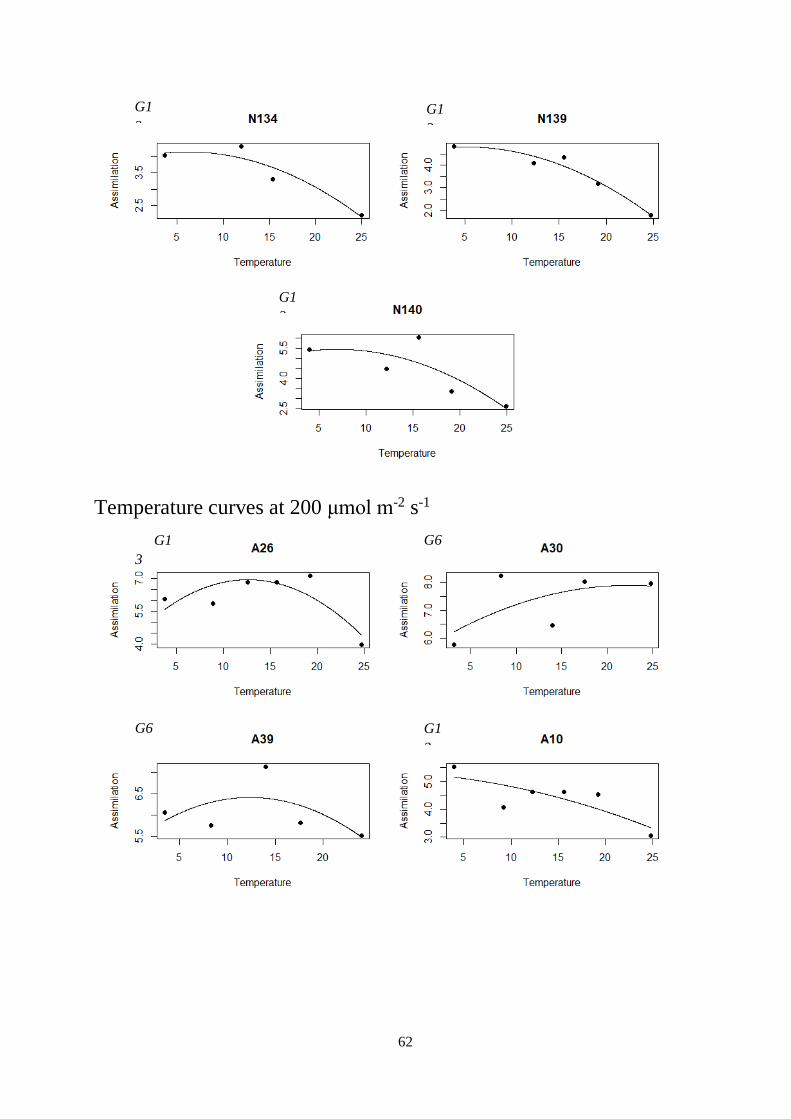
62
Temperature curves at 200 μmol m-2 s-1
G1
3
G1
3
G1
3
G1
3
G1
3
G6
G6

63
G1
3
G6
G1
3
G6
G1
3
G1
3
G1
3
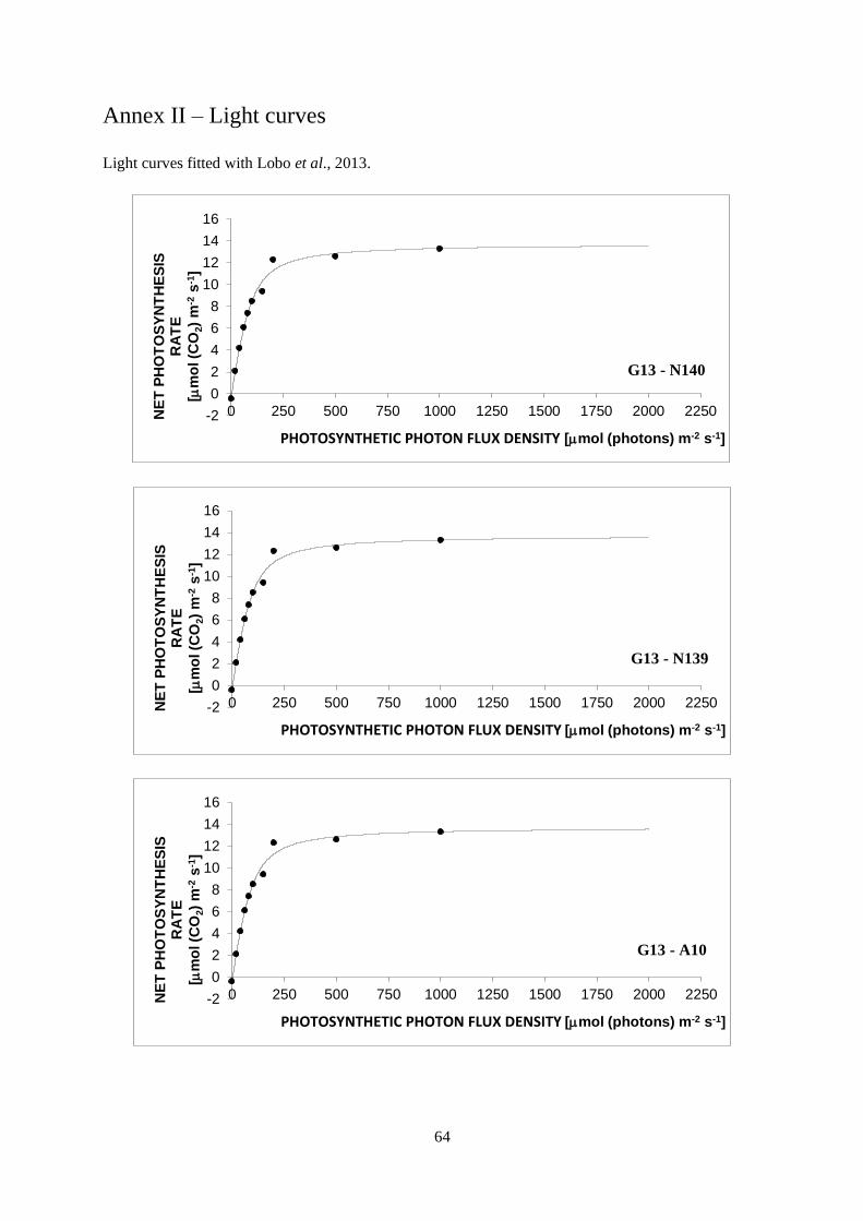
64
Annex II – Light curves
Light curves fitted with Lobo et al., 2013.
-2
0
2
4
6
8
10
12
14
16
0 250 500 750 1000 1250 1500 1750 2000 2250NE
T P
HO
TO
SY
NT
HE
SIS
R
AT
E
[mm
ol (C
O2)
m-2
s-1
]
PHOTOSYNTHETIC PHOTON FLUX DENSITY [mmol (photons) m-2 s-1]
G13 - N140
-2
0
2
4
6
8
10
12
14
16
0 250 500 750 1000 1250 1500 1750 2000 2250NE
T P
HO
TO
SY
NT
HE
SIS
R
AT
E
[mm
ol (C
O2)
m-2
s-1
]
PHOTOSYNTHETIC PHOTON FLUX DENSITY [mmol (photons) m-2 s-1]
G13 - N139
-2
0
2
4
6
8
10
12
14
16
0 250 500 750 1000 1250 1500 1750 2000 2250NE
T P
HO
TO
SY
NT
HE
SIS
R
AT
E
[mm
ol (C
O2)
m-2
s-1
]
PHOTOSYNTHETIC PHOTON FLUX DENSITY [mmol (photons) m-2 s-1]
G13 - A10
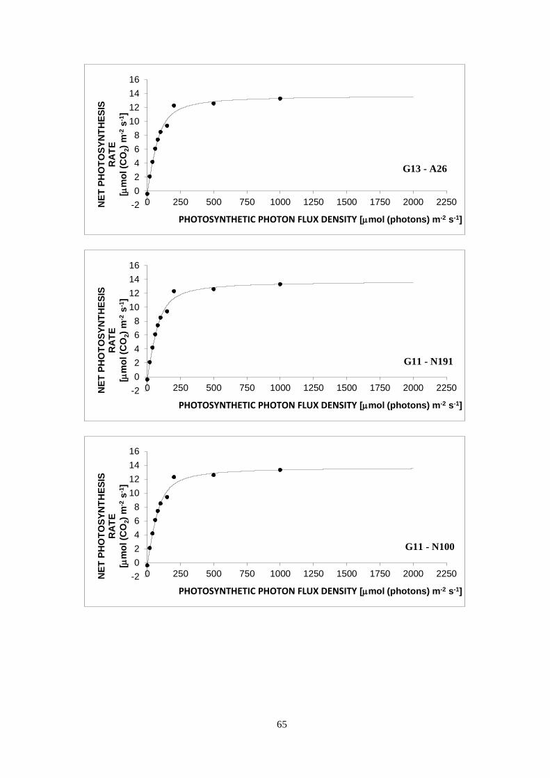
65
-2
0
2
4
6
8
10
12
14
16
0 250 500 750 1000 1250 1500 1750 2000 2250NE
T P
HO
TO
SY
NT
HE
SIS
R
AT
E
[mm
ol (C
O2)
m-2
s-1
]
PHOTOSYNTHETIC PHOTON FLUX DENSITY [mmol (photons) m-2 s-1]
G13 - A26
-2
0
2
4
6
8
10
12
14
16
0 250 500 750 1000 1250 1500 1750 2000 2250NE
T P
HO
TO
SY
NT
HE
SIS
R
AT
E
[mm
ol (C
O2)
m-2
s-1
]
PHOTOSYNTHETIC PHOTON FLUX DENSITY [mmol (photons) m-2 s-1]
G11 - N191
-2
0
2
4
6
8
10
12
14
16
0 250 500 750 1000 1250 1500 1750 2000 2250NE
T P
HO
TO
SY
NT
HE
SIS
R
AT
E
[mm
ol (C
O2)
m-2
s-1
]
PHOTOSYNTHETIC PHOTON FLUX DENSITY [mmol (photons) m-2 s-1]
G11 - N100

66
-2
0
2
4
6
8
10
12
14
16
0 250 500 750 1000 1250 1500 1750 2000 2250NE
T P
HO
TO
SY
NT
HE
SIS
R
AT
E
[mm
ol (C
O2)
m-2
s-1
]
PHOTOSYNTHETIC PHOTON FLUX DENSITY [mmol (photons) m-2 s-1]
G11 - A70
-2
0
2
4
6
8
10
12
14
16
0 250 500 750 1000 1250 1500 1750 2000 2250NE
T P
HO
TO
SY
NT
HE
SIS
R
AT
E
[mm
ol (C
O2)
m-2
s-1
]
PHOTOSYNTHETIC PHOTON FLUX DENSITY [mmol (photons) m-2 s-1]
G11 - A41
-2
0
2
4
6
8
10
12
14
16
0 250 500 750 1000 1250 1500 1750 2000 2250NE
T P
HO
TO
SY
NT
HE
SIS
R
AT
E
[mm
ol (C
O2)
m-2
s-1
]
PHOTOSYNTHETIC PHOTON FLUX DENSITY [mmol (photons) m-2 s-1]
G9 - N131
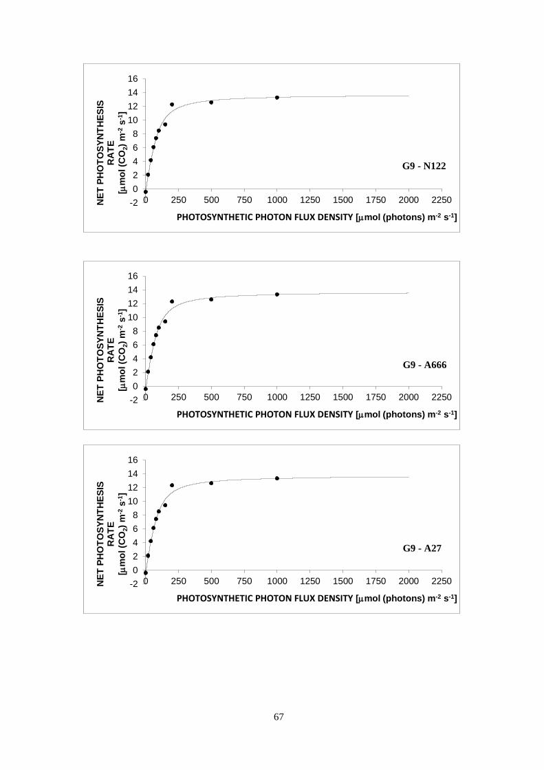
67
-2
0
2
4
6
8
10
12
14
16
0 250 500 750 1000 1250 1500 1750 2000 2250NE
T P
HO
TO
SY
NT
HE
SIS
R
AT
E
[mm
ol (C
O2)
m-2
s-1
]
PHOTOSYNTHETIC PHOTON FLUX DENSITY [mmol (photons) m-2 s-1]
G9 - N122
-2
0
2
4
6
8
10
12
14
16
0 250 500 750 1000 1250 1500 1750 2000 2250NE
T P
HO
TO
SY
NT
HE
SIS
R
AT
E
[mm
ol (C
O2)
m-2
s-1
]
PHOTOSYNTHETIC PHOTON FLUX DENSITY [mmol (photons) m-2 s-1]
G9 - A666
-2
0
2
4
6
8
10
12
14
16
0 250 500 750 1000 1250 1500 1750 2000 2250NE
T P
HO
TO
SY
NT
HE
SIS
R
AT
E
[mm
ol (C
O2)
m-2
s-1
]
PHOTOSYNTHETIC PHOTON FLUX DENSITY [mmol (photons) m-2 s-1]
G9 - A27

68
-2
0
2
4
6
8
10
12
14
16
0 250 500 750 1000 1250 1500 1750 2000 2250NE
T P
HO
TO
SY
NT
HE
SIS
R
AT
E
[mm
ol (C
O2)
m-2
s-1
]
PHOTOSYNTHETIC PHOTON FLUX DENSITY [mmol (photons) m-2 s-1]
G6 - N127
-2
0
2
4
6
8
10
12
14
16
0 250 500 750 1000 1250 1500 1750 2000 2250NE
T P
HO
TO
SY
NT
HE
SIS
R
AT
E
[mm
ol (C
O2)
m-2
s-1
]
PHOTOSYNTHETIC PHOTON FLUX DENSITY [mmol (photons) m-2 s-1]
G6 - N119
-2
0
2
4
6
8
10
12
14
16
0 250 500 750 1000 1250 1500 1750 2000 2250NE
T P
HO
TO
SY
NT
HE
SIS
R
AT
E
[mm
ol (C
O2)
m-2
s-1
]
PHOTOSYNTHETIC PHOTON FLUX DENSITY [mmol (photons) m-2 s-1]
G6 - A39

69
-2
0
2
4
6
8
10
12
14
16
0 250 500 750 1000 1250 1500 1750 2000 2250NE
T P
HO
TO
SY
NT
HE
SIS
R
AT
E
[mm
ol (C
O2)
m-2
s-1
]
PHOTOSYNTHETIC PHOTON FLUX DENSITY [mmol (photons) m-2 s-1]
G6 - A30
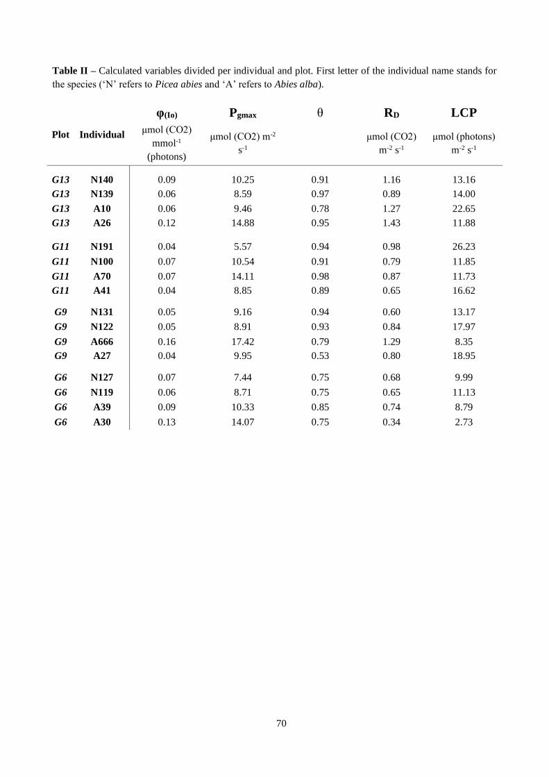
70
Table II – Calculated variables divided per individual and plot. First letter of the individual name stands for
the species (‘N’ refers to Picea abies and ‘A’ refers to Abies alba).
Plot Individual
φ(Io) Pgmax θ RD LCP
μmol (CO2)
mmol-1
(photons)
μmol (CO2) m-2
s-1 μmol (CO2)
m-2 s-1
μmol (photons)
m-2 s-1
G13 N140 0.09 10.25 0.91 1.16 13.16
G13 N139 0.06 8.59 0.97 0.89 14.00
G13 A10 0.06 9.46 0.78 1.27 22.65
G13 A26 0.12 14.88 0.95 1.43 11.88
G11 N191 0.04 5.57 0.94 0.98 26.23
G11 N100 0.07 10.54 0.91 0.79 11.85
G11 A70 0.07 14.11 0.98 0.87 11.73
G11 A41 0.04 8.85 0.89 0.65 16.62
G9 N131 0.05 9.16 0.94 0.60 13.17
G9 N122 0.05 8.91 0.93 0.84 17.97
G9 A666 0.16 17.42 0.79 1.29 8.35
G9 A27 0.04 9.95 0.53 0.80 18.95
G6 N127 0.07 7.44 0.75 0.68 9.99
G6 N119 0.06 8.71 0.75 0.65 11.13
G6 A39 0.09 10.33 0.85 0.74 8.79
G6 A30 0.13 14.07 0.75 0.34 2.73
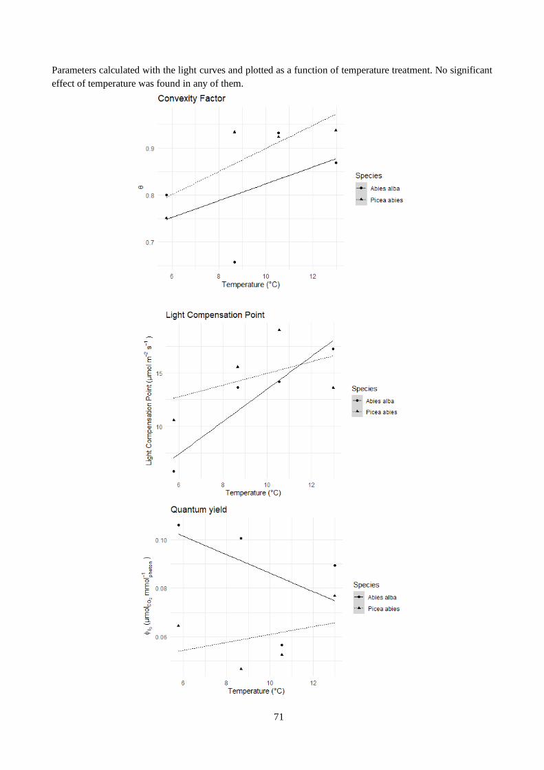
71
Parameters calculated with the light curves and plotted as a function of temperature treatment. No significant
effect of temperature was found in any of them.

72
Annex III – Growth Divided by temperature treatment.
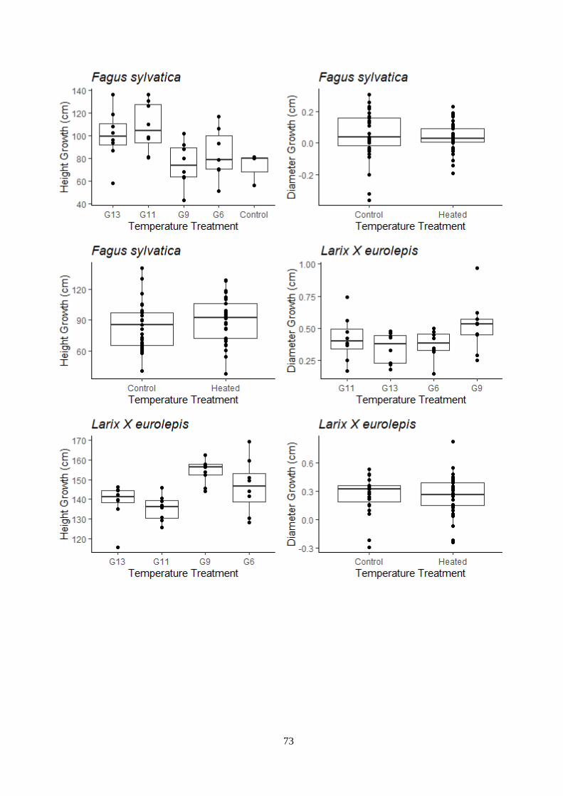
73
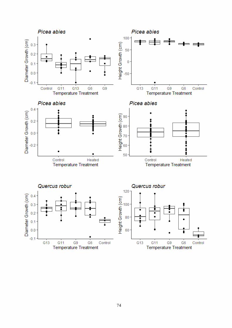
74
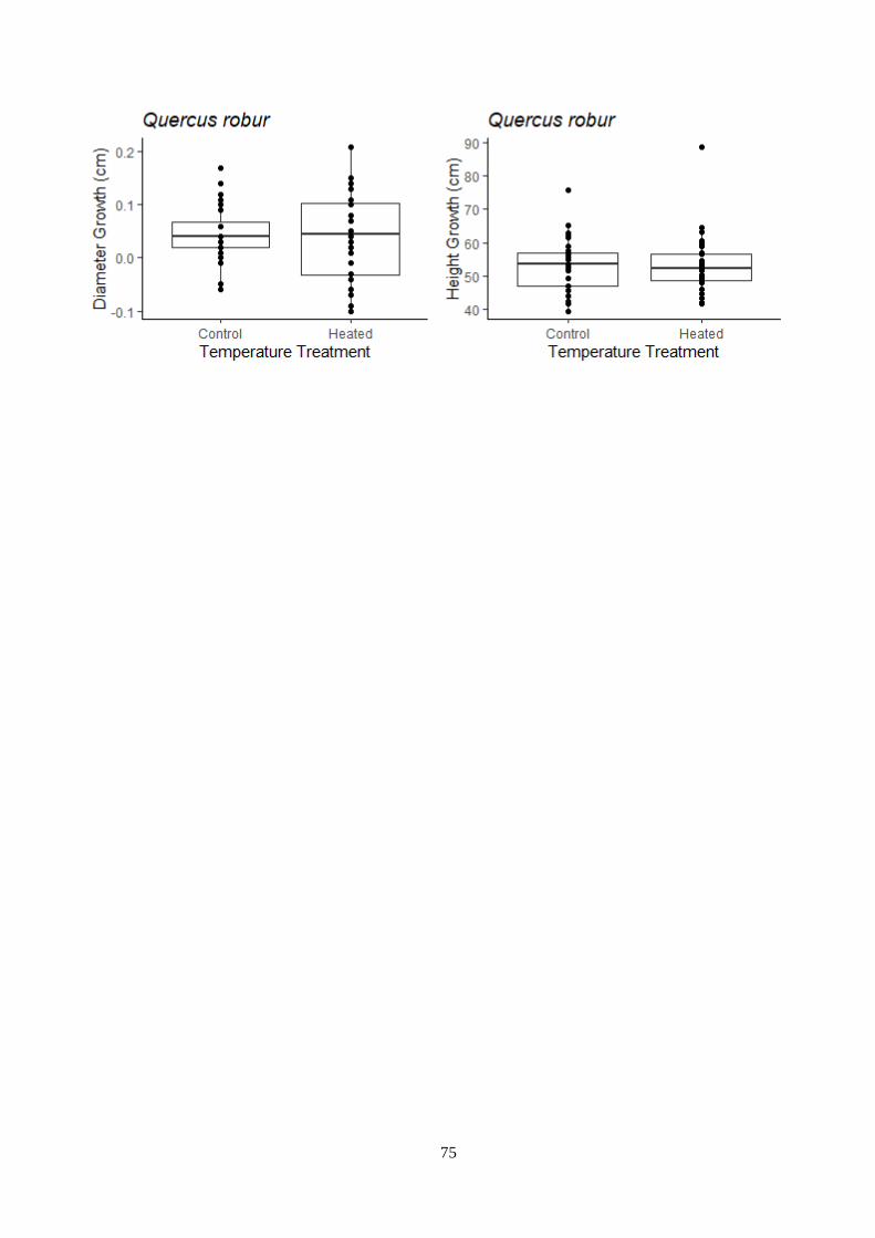
75

76
Growth analysis divided by light treatment.
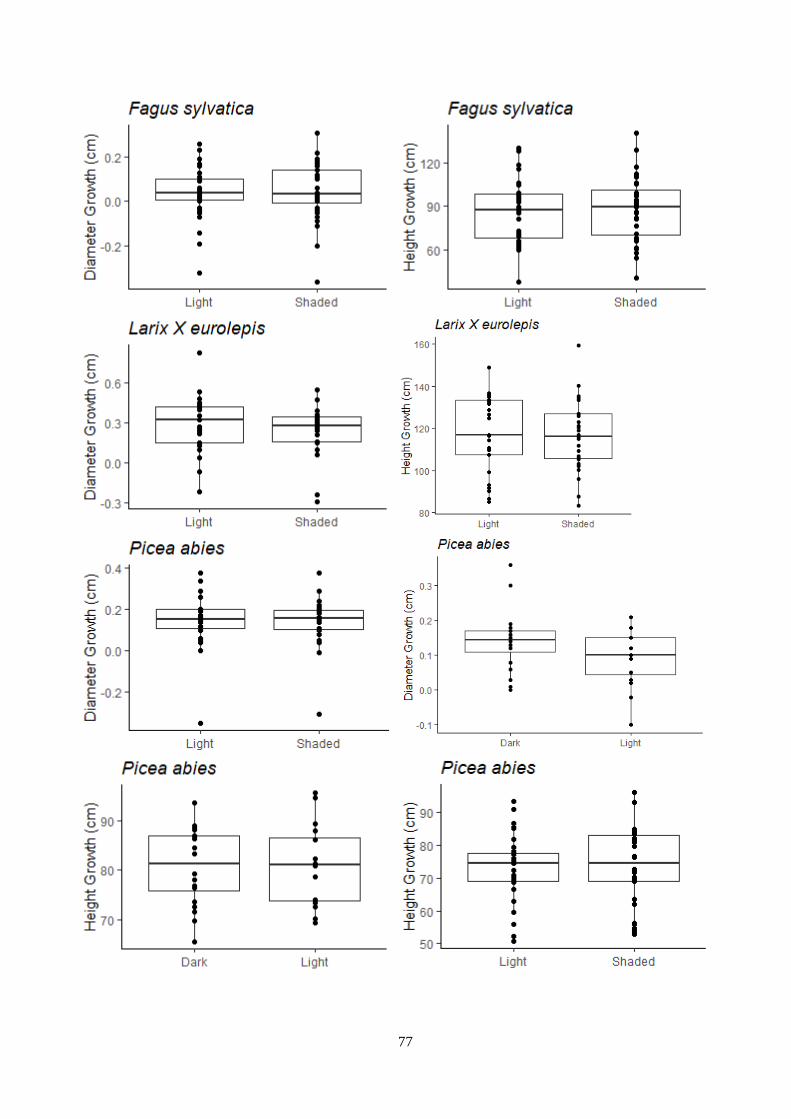
77
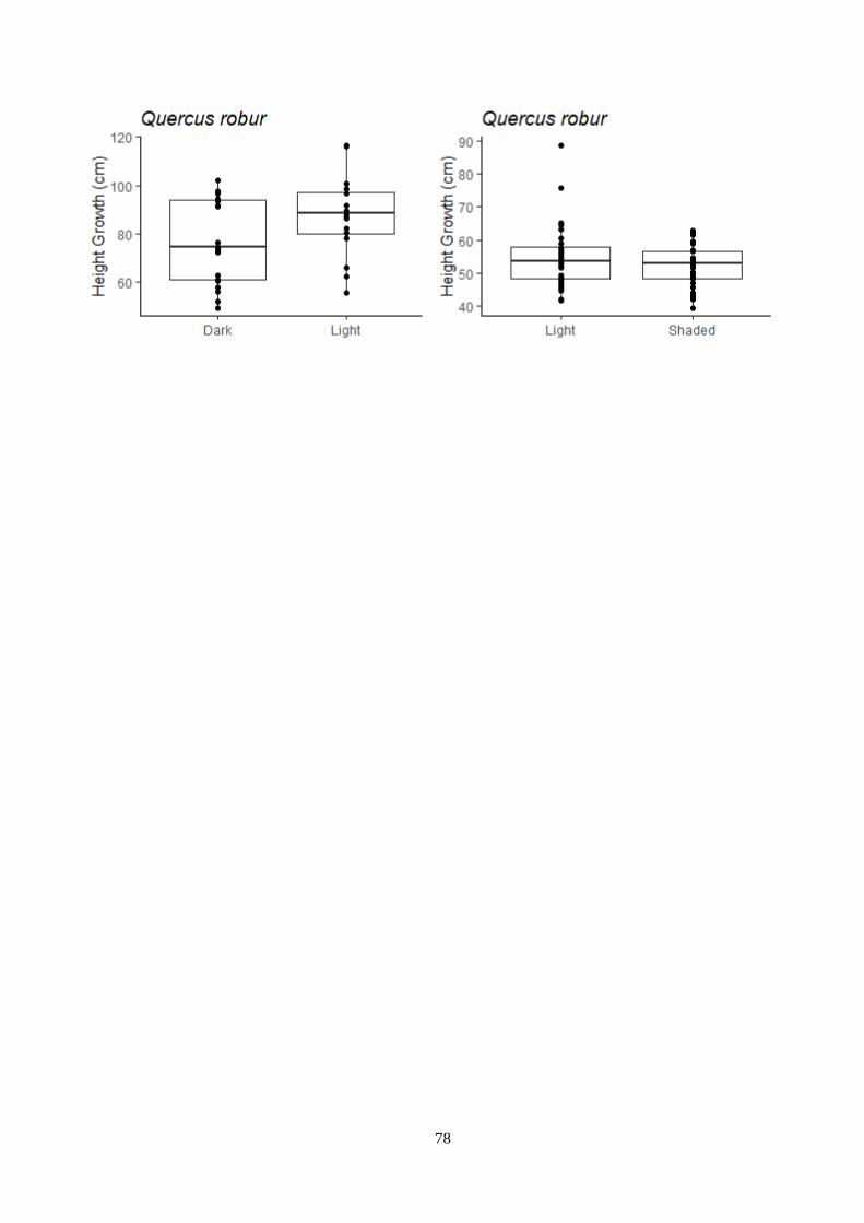
78