Wind Turning in The Atmospheric Boundary...

Time [HH:MM]

Height[m

]

40

60

80

100

120

140

160

180

200

0 200 400 600 800 1000 1200 1400 1600 1800 2000 22002300

0

2

4

6

8

10

Wind Turning in The Atmospheric Boundary LayerMaster’s thesis in Physics and Astronomy

GHAZAL TORABI

Department of Fundamental PhysicsDivision of Physics and AstronomyCHALMERS UNIVERSITY OF TECHNOLOGYGoteborg, Sweden 2013Master’s thesis 2013:68

MASTER’S THESIS IN PHYSICS AND ASTRONOMY

Wind Turning in The Atmospheric Boundary Layer

GHAZAL TORABI

Department of Fundamental PhysicsDivision of Physics and Astronomy

CHALMERS UNIVERSITY OF TECHNOLOGY

Goteborg, Sweden 2013

Wind Turning in The Atmospheric Boundary LayerGHAZAL TORABI

c© GHAZAL TORABI, 2013

Master’s thesis 2013:68ISSN 1652-8557Department of Fundamental PhysicsDivision of Physics and AstronomyChalmers University of TechnologySE-412 96 GoteborgSwedenTelephone: +46 (0)31-772 1000

Cover:A contour plot of an average diurnal wind turning from height 40 to 200 m by lidar observations

Chalmers ReproserviceGoteborg, Sweden 2013

Wind Turning in The Atmospheric Boundary LayerMaster’s thesis in Physics and AstronomyGHAZAL TORABIDepartment of Fundamental PhysicsDivision of Physics and AstronomyChalmers University of Technology

Abstract

Measurements at Høvsøre site in Denmark are used to analyse the change with height of wind speed and theturning of the wind in the atmospheric boundary layer. The purpose is to study the behaviour of wind turningand wind shear and analyse the relations between them.

The study will show the effect of wide range of stability classes on the turning of wind and wind speedby combining cup, wind vane and sonic at meteorological mast with lidar observations. Easterly wind isinvestigated at Høvsøre site to study the behaviour of the overland wind shear and wind turning from November2008 to April 2009. In this study, data are analysed based on average 10-min wind speeds and wind directionsdiurnal, monthly and during the whole period of measurements.

The results show that first, the wind speed profile of meteorological mast and lidar are in agreement todifferent stability classes. Second, the wind direction profile changes with height reasonable in all stabilityconditions except in very unstable and unstable cases. Third result shows that the wind shear and the windturning are unstable during the day and stable during the night in the average whole period of six months.Fourth, the yearly wind turning and wind shear are in agreement without considering lidar observations. Theybehave also in similar way when lidar observations combine with meteorological mast. In conclusion, thecomparisons between the wind shear and the turning of the wind with and without considering lidar observationshow that the wind shear is in the agreement with the wind turning.

The second result on this study was unexpected. The reason for this behaviour may be explained as thenumber of measurements are very low. Another reason is that the value of heat fluxes are low, whereas theyhave to be high. The last reason might be related to a baroclinicity.

Keywords: Wind shear, Surface layer, Turbulence

i

Preface

This thesis was prepared at the department of Wind Energy at the Technical University of Denmark in fulfilmentof the requirements for acquiring an M.Sc. in Physics and Astronomy. This master thesis was conducted duringthe final year of my two years Master of Science program in Physics and Astronomy. My work has been carriedout in the Meteorological section at the DTU wind energy - Risø; under the supervision of Jacob Berg. AlfredoPena served as co-supervisor.

This thesis deals with the changes in the wind speed and the wind direction in the atmospheric boundarylayer by combining cup, sonic and vane at meteorological mast with lidar observations overland at Høvsøre,Denmark. This study is carried out by averaging the 10-min wind speed and wind direction measurements inthe wide range of atmospheric stability conditions from November 2008 to April 2009.

This thesis includes 7 main sections. Section 1 is the introduction. Section 2 provides a review of the maincharacteristics of the atmospheric boundary layer, including the effect of stability and turbulence in the surface.It also shows how the analysis of the turning of the wind has been performed. Section 3 provides a descriptionof the Høvsøre site in Denmark and the instrumentation used in this study. Section 4 explains data filteringand data averaging. Section 5 provides the results from the analysis of both wind shear and the turning of thewind. Discussion and conclusions are provided in the last two sections.

Acknowledgements

It is a pleasure to thank those who made this thesis possible. I give my thanks to my supervisor, Jacob Bergwho gave me the opportunity to do my thesis at Risø. He reviewed my works and always provided valuableadvice as and when required. I would like to thank to my co-supervisor, Alfredo Pena who always explainedand taught me with patience. He gave me regular feedback and encouraged me to improve my work.

Thanks to my coordinator, Gabriele Ferretti at Chalmers University of Technology for his help and permissionto continue my study in wind energy. A note of thanks to Martin Otto Laver Hansen for supporting me tostudy at Technical University of Denmark. I would like to thank my great teacher, Uwe Schmidt Paulsen forhelping me improve my knowledge.

I would be lacking in gratitude if I do not thank my friends. When I was down, they were always there topick me up.

My grateful goes to my family in Denmark, that made me feel secured and cared for.Finally, I would like to thank my family in Iran for their constant supports and pure love in entire of my

life, specially my aunt. I could not move and study abroad without my aunt’s (Farzaneh) supports.

iii

Contents

Abstract i

Preface iii

Acknowledgements iii

Contents v

1 Introduction 4

2 Theory 52.1 The Atmospheric Boundary Layer . . . . . . . . . . . . . . . . . . . . . . . . . . . . . . . . . . . . 52.2 The Surface Layer . . . . . . . . . . . . . . . . . . . . . . . . . . . . . . . . . . . . . . . . . . . . . 62.3 The Ekman Spiral . . . . . . . . . . . . . . . . . . . . . . . . . . . . . . . . . . . . . . . . . . . . . 7

3 Site and Instrumentation 83.1 Høvsøre . . . . . . . . . . . . . . . . . . . . . . . . . . . . . . . . . . . . . . . . . . . . . . . . . . . 83.2 Instrumentation . . . . . . . . . . . . . . . . . . . . . . . . . . . . . . . . . . . . . . . . . . . . . . 83.2.1 Lidar . . . . . . . . . . . . . . . . . . . . . . . . . . . . . . . . . . . . . . . . . . . . . . . . . . . 83.2.2 Cup and Vane . . . . . . . . . . . . . . . . . . . . . . . . . . . . . . . . . . . . . . . . . . . . . . 93.2.3 Sonic . . . . . . . . . . . . . . . . . . . . . . . . . . . . . . . . . . . . . . . . . . . . . . . . . . . 10

4 Data Treatment 114.1 Data Filtering . . . . . . . . . . . . . . . . . . . . . . . . . . . . . . . . . . . . . . . . . . . . . . . . 114.2 Data Averaging . . . . . . . . . . . . . . . . . . . . . . . . . . . . . . . . . . . . . . . . . . . . . . . 11

5 Results 145.1 The effect of stability . . . . . . . . . . . . . . . . . . . . . . . . . . . . . . . . . . . . . . . . . . . 155.1.1 Vertical Wind Shear . . . . . . . . . . . . . . . . . . . . . . . . . . . . . . . . . . . . . . . . . . . 155.1.2 Wind Turning . . . . . . . . . . . . . . . . . . . . . . . . . . . . . . . . . . . . . . . . . . . . . . 165.2 Monthly Evolution . . . . . . . . . . . . . . . . . . . . . . . . . . . . . . . . . . . . . . . . . . . . . 215.2.1 Vertical Wind Shear . . . . . . . . . . . . . . . . . . . . . . . . . . . . . . . . . . . . . . . . . . . 215.2.2 Wind Turning . . . . . . . . . . . . . . . . . . . . . . . . . . . . . . . . . . . . . . . . . . . . . . 225.3 Daily Evolution . . . . . . . . . . . . . . . . . . . . . . . . . . . . . . . . . . . . . . . . . . . . . . . 235.3.1 Vertical Wind Shear . . . . . . . . . . . . . . . . . . . . . . . . . . . . . . . . . . . . . . . . . . . 235.3.2 Wind Turning . . . . . . . . . . . . . . . . . . . . . . . . . . . . . . . . . . . . . . . . . . . . . . 245.4 Non-dimensionalization . . . . . . . . . . . . . . . . . . . . . . . . . . . . . . . . . . . . . . . . . . 285.4.1 Vertical Wind Shear . . . . . . . . . . . . . . . . . . . . . . . . . . . . . . . . . . . . . . . . . . . 285.4.2 Wind Turning . . . . . . . . . . . . . . . . . . . . . . . . . . . . . . . . . . . . . . . . . . . . . . 28

6 Discussion 32

7 Conclusion 33

References 34

v

List of Figures

2.1 The evolution of the atmospheric boundary layer with height during an ideal daily cycle. CBL and SBL

are convective boundary layer and stable boundary layer respectively. z is the height from the ground

and zi is the boundary layer height [Pen09]. . . . . . . . . . . . . . . . . . . . . . . . . . . . . . . . 52.2 The logarithmic behaviour of the wind profile in three stability conditions in the surface layer, z0=0.1 m

[Pen09]. . . . . . . . . . . . . . . . . . . . . . . . . . . . . . . . . . . . . . . . . . . . . . . . . . 62.3 The Ekman Spiral. u and v are the longitudinal and latitudinal components of wind speed. ug and vg

are the longitudinal and latitudinal components of the geostrophic wind [Etl02]. . . . . . . . . . . . . 73.1 Høvsøre national test centre for large wind turbines at Denmark. Light tower and meteorological mast

are shown in the figure. 5 white dots are wind turbines. . . . . . . . . . . . . . . . . . . . . . . . . . 83.2 Measurement process of the wind lidar. w0 and ∆f are frequency of light and Doppler shift, respectively.

d shows the distance between a target and a laser. The moving target distance is shown by d′ [Pen09]. 93.3 Retrieving the wind speed components in lidar WindCube. u, v and w are the wind speed components.

Vh and Dir show the horizontal wind speed and wind direction, respectively [Car13a]. . . . . . . . . . 104.1 Wind rose at Høvsøre site. It is observed at height 100 m between November 2008 and April 2009.

Legend corresponds to wind speed in m/s. . . . . . . . . . . . . . . . . . . . . . . . . . . . . . . . . 125.1 Correlations for different CNR values between lidar and cup wind speeds at height 100 m (left panel),

and between lidar and vane wind directions at height 100 m (right). . . . . . . . . . . . . . . . . . . 145.2 The number of data for different CNR values between lidar and cup wind speeds at height 100 m (left

panel), and between lidar and vane wind directions at height 100 m (right). . . . . . . . . . . . . . . 145.3 Regression for mean wind speeds at heights 60 m (red dots) and 100 m (blue dots) in lidar, cup and

sonic. At each height regression slope, offset and regression coefficient are calculated. . . . . . . . . . 155.4 Regression for mean wind direction at heights 60 m (red dots) and 100 m (blue dots) in lidar, vane and

sonic, and at heights 10 m (green dots) between vane and sonic. Regression slope, offset and regression

coefficient are calculated for each heights. . . . . . . . . . . . . . . . . . . . . . . . . . . . . . . . . 165.5 Wind profile of lidar (top left), cup (top right) and sonic (on the bottom) in different stability classes.

Legend information is given in Table 5.1. . . . . . . . . . . . . . . . . . . . . . . . . . . . . . . . . 175.6 Comparison of lidar, cup and sonic wind profile at different stability classes and heights. Lidar shows

with plus sign, sonic with square and cup with circle. Different colors are related to different stability. 185.7 The wind direction changes with heights in various stability classes in lidar (top left), vane (top right)

and sonic (on the bottom). ∆θ indicates the difference in wind direction in each instrument from

reference vane wind direction at height 10 m. . . . . . . . . . . . . . . . . . . . . . . . . . . . . . . 185.8 Error bers of the wind turning behaviour in lidar in seven stability classes. The top (left) plot consists

of very stable, neutral and very unstable wind. Stable and unstable wind error bars are shown on the

top (right). Near stable and near unstable are on the bottom of the figure. . . . . . . . . . . . . . . . 195.9 Error bars of the wind turning behaviour in vane in seven stability classes. The top (left) plot consists

of very stable, neutral and very unstable wind. Stable and unstable wind error bar is shown on the top

(right). Near stable and near unstable are on the bottom of the figure. . . . . . . . . . . . . . . . . 195.10 Error bars of the wind turning behaviour in sonic in seven stability classes. The top (left) plot consists

of very stable, neutral and very unstable wind. Stable and unstable wind error bars are shown one the

top (right). Near stable and near unstable are on the bottom of the figure. . . . . . . . . . . . . . . 205.11 The comparison of lidar, vane and sonic wind turning at different stabilities and heights. ∆θ indicates

the difference in wind direction in each instrument from reference vane wind direction at height 10

m. Lidar shows with plus sign, sonic with square and vane with circle. Different colors are related to

different stability classes. . . . . . . . . . . . . . . . . . . . . . . . . . . . . . . . . . . . . . . . . . 215.12 Wind shear in lidar, cup and sonic from December 2008 to April 2009 (left). ∆U indicates the difference

in wind speed of each instrument from reference sonic wind speed at height 10 m. The figure (right) is

sonic and cup wind shear without considering lidar during 12 months (from November 2008 to October

2009). Error bars of both cases are shown in the figure. . . . . . . . . . . . . . . . . . . . . . . . . . 225.13 Wind turning behaviour in lidar, vane and sonic from December 2008 to April 2009 (left). ∆θ indicates

the difference in wind direction in each instrument from reference vane wind direction at height 10 m.

The figure (right) is sonic and vane wind turning without considering lidar during 12 months (from

November 2008 to October 2009). Error bars of both cases are shown in the figure. . . . . . . . . . . 225.14 The amount of data that is classified by months and each stability classes. Different colors are related

to each stability conditions. . . . . . . . . . . . . . . . . . . . . . . . . . . . . . . . . . . . . . . . 23

1

5.15 Average diurnal comparison of lidar, cup and sonic wind shear from November 2008 to April 2009. ∆U

indicates the difference in wind speed of each instrument from reference sonic wind speed at height 10

m. Error bars of the diurnal behaviour of three instruments are shown in this figure. . . . . . . . . . 245.16 Lidar, cup and sonic wind shear behaviour on December, January, February, March and April during

average 24 hours. ∆U indicates the difference in wind speed of each instrument from reference sonic

wind speed at height 10 m. Error bars of wind shear behaviour in lidar, cup and sonic are shown in the

figure. . . . . . . . . . . . . . . . . . . . . . . . . . . . . . . . . . . . . . . . . . . . . . . . . . . 255.17 Average diurnal comparison of lidar, vane and sonic wind turning from November 2008 to April 2009.

∆θ indicates the difference in wind direction in each instrument from reference vane wind direction at

height 10 m. Error bars of the diurnal behaviour of three instruments are shown in this figure. . . . . 265.18 Lidar, vane and sonic wind turning behaviour on December, January, February, March and April during

average 24 hours. ∆θ indicates the difference in wind direction in each instrument from reference vane

wind direction at height 10 m. Error bars in mean diurnal wind turning behaviour in lidar, vane and

sonic are shown in this figure. . . . . . . . . . . . . . . . . . . . . . . . . . . . . . . . . . . . . . . 275.19 Collapsing of lidar, cup and sonic wind speed variation in different stability classes. . . . . . . . . . . 295.20 the combonation of the collapsed data of lidar, cup and sonic wind speed variation in different stability

classes from November 2008 to April 2009. z/zi is logarithmic . . . . . . . . . . . . . . . . . . . . . 305.21 Fitting of non-dimensionalized data in lidar, cup and sonic. . . . . . . . . . . . . . . . . . . . . . . . 305.22 Non-dimensionalization of lidar, vane and sonic wind turning variation in different stability classes. ∆θ

indicates the difference in wind direction in each instrument from reference vane wind direction at height

10 m. . . . . . . . . . . . . . . . . . . . . . . . . . . . . . . . . . . . . . . . . . . . . . . . . . . . 31

List of Tables

4.1 Filtering of data . . . . . . . . . . . . . . . . . . . . . . . . . . . . . . . . . . . . . . . . . . . . 124.2 The results of mean and standard deviation in two different methods . . . . . . . . . . . . . . 135.1 Different stability classes according to Obukhov length [Pen09] . . . . . . . . . . . . . . . . . . 155.2 Value of zi for different stability classes after non-dimensionalization. . . . . . . . . . . . . . . . 28

2

Notation

d focused distance

d′ distance from laser source to targets in air

u∗ friction velocity

w0 angular frequency of light

∆f Doppler shift

γ latitudinal component of geostrophic wind

∂ partial derivative

θ wind direction

θ′ potential temperature

λl wavelength of light

φ the angle when the laser beam tilt from the zenith

ψm diabatic correction of the logarithmic wind profile

σθ standard deviation

ϕm dimensionless wind shear

ϕ along-beam weighting function

Dir horizontal wind direction

g gravitational acceleration

KM turbulent exchange coefficient for momentum

Q0 heat flux

R2 determination coefficient

T0 surface air temperature

ug longitudinal component of geostrophic wind

vg latitudinal component of geostrophic wind

Vh horizontal wind speed

vr radial velocity

z0 roughness length

zi height of boundary layer

f Coriolis parameter

k von Karman constant

L Obukhov length

n number of measurements

U mean wind speed

u longitudinal component of wind speed

v latitudinal component of wind speed

w vertical component of wind speed

z height above the ground

ABL Atmospheric boundary layer

CBL Convective boundary layer

DBS Doppler beam swinging

SBL Stable boundary layer

VAD velocity azimuth display

3

1 Introduction

The behaviour of the atmospheric flow close to the ground’s surface is a main concern in wind energy [BMN13].The ground’s surface has an effect on the wind characteristics even at altitudes above 100 m [Ass00]. The windis influenced by roughness, roughness changes, terrain, and obstacles, as many of these terrain and surfacecharacteristics add/subtract drag to the flow. Hence, the wind speed and wind direction profile at variousheights above the ground level depend on the surface topology, atmospheric stability and changes in time.[DN09].

Wind turbines have increased in size in the last two decades due to high demand for wind power. Thisgrowing in size causes environmental and economical impacts. From the economic point of view, the cost ofenergy has decreased. The reason is that the industries have based their investments on acknowledge componentof the power generation which in the wind energy depends on the wind characteristics [Ass+09]. Atmosphericstability can affect the wind speed and wind direction thus affecting power generation. This impact has haddifferent results in several studies. For example, Rareshide et al (2009) found high wind shear (stable condition)makes the higher power production than low wind shear (unstable condition) at a US plains wind farm [Rar+09].In contrast, Wagner et al (2009) found high wind shear lead to lower power than low wind shear in the flatDanish terrain [Wag+09],[WL12].

Atmospheric turbulence can have significant effects on the turbines and environment. It affects turbineloads through fatigue and wake effects. In a wind farm, turbines themselves create turbulence in their wakesand this turbulence is added to atmospheric turbulence and increases the load. Another impact is related tothe increase in propagation of noise from the wind turbines themselves. Under unstable conditions, strongturbulence creates background noise near the ground surface and so the noise from the turbines is negligible.By contrast, the turbine noise is heard more clearly in the stable condition [LC12].

The large turbines cause meteorological features which have not been considered in the past are playing amain role. For instance, the vertical gradient of mean wind speed or the analysis of the wind turning has notbeen include in many studies [Etl02]. In particular, the wind turning has not been so important as people tendto believe that close to the surface the wind does not turn too much. However, with the modern wind turbines,wind turning may be as important as the wind shear. The vertical wind profile varies through time and spaceand so it is important to observe the wind characteristics as accurately as possible [DN09]. Furthermore,collecting wind information from these tall turbines need new techniques, i.e. remote sensors, because theinstallation of the meteorological mast above 80 m becomes expensive. By measuring with different instruments,part of the uncertainty of the results of the analysis can be evaluated as the three types of the instrumentsobserve the wind speed and wind direction in a different manner.

Accurate prediction of the wind speed and the wind direction is extremely important for the wind energyindustry. For example, high accuracy decreases the uncertainty of the predicted energy production [Ass+09].If wind conditions evolve differently than expected, companies face financial losses, production and salesdifficulties.

The main goal of this project, which has been carried out at DTU Wind Energy, Risø campus, is to studythe variation with height (i.e. the vertical profile) of both the turning of the wind and the vertical wind speedin the atmospheric boundary layer from the analysis of cup and sonic anemometer measurements combinedwith wind lidar observations at a flat area known as Høvsøre in Western Denmark. The vertical wind speedprofiles and profiles of the wind turning are analysed under a wide range of atmospheric stability conditionsfor the different instruments as it has been observed that these profiles show distinctive shape and behaviourdepending on the atmospheric turbulence characteristics [Sat+12], [SM09].

This thesis includes 7 main sections. Section 2 provides a review of the main characteristics of the atmosphericboundary layer, including the effect of stability and turbulence on the surface. It also shows how the analysisof the turning of the wind has been performed. Section 3 provides a description of the Høvsøre site in Denmarkand the instrumentation used in this study. Section 4 explains about the data filtering and data averaging.Section 5 provides the results of the analysis of both wind shear and the turning of the wind. Discussion andconclusions are provided in the last two sections.

4

2 Theory

2.1 The Atmospheric Boundary Layer

The atmospheric boundary layer (ABL) is a part of the troposphere. The ABL is affected by turbulence motionand so its thickness varies between a hundred meter to a few kilometres [Stu88]. The characteristics of thislayer are different during the day, in particular when it is warm, than during the night. This difference isexplained firstly by wind shear, which is produced by friction of the wind with the surface, and secondly by theheat flux that is caused by the differences of temperature of the air layers and the surface. There are threemain different turbulence regimes in which the atmospheric flow is commonly classified when the boundarylayer is assumed to be homogeneous:

1. Convective or unstable: This occurs when the heat is transferred from the warm surface to the colderatmosphere. During the day the surface is warmer than the atmosphere, and the difference in density betweenthe warm and the cold air gives rise to buoyancy forces in the atmosphere, causing unstable condition. Thus, thevertical motion in unstable atmosphere is large and the thickness of the layer reaches to one or two kilometres[Pen09].

2. Neutral: This condition dominates when there is no net heat flux in the atmosphere, but with highfriction velocity. It means that the wind speed is high near the surface [Pen09]. Neutral condition is betweenunstable and stable conditions. It happens usually in the cloudy weather when strong surface heating andcooling do not occur [Sys13].

3. Stable: It is dominating when the surface is cool and there is a high wind shear. At night the surfaceis colder than the atmosphere and the colder air wants to stay in its position. The stable condition is alsofound over ice and snow that cover the surfaces. The vertical motion in the stable atmosphere happens rarely.Therefore, the thickness of layer is around a hundred meter [Pen09].

Figure 2.1 shows the structure of the ABL during 24 hours. It consists of the surface layer, convectiveboundary layer (CBL), stable boundary layer (SBL), residual layer and entrainment zone. Unstable conditionis dominating in the CBL and happens during the day. Besides, converting potential energy to kinetic energycauses an increase in the turbulence level. In the SBL, the temperature and wind speed are not constantcontrary to CBL, and the the height of SBL is determined when the smaller eddies reach to the residual layer.Residual layer is located on the top of this layer which is made by CBL and the entrainment zone. In addition,the entrainment zone comes from the interaction of free stable atmosphere and CBL layer. The inversionhappens in this part because the temperature and height have direct proportion [Pen09].

Figure 2.1: The evolution of the atmospheric boundary layer with height during an ideal daily cycle. CBL and SBL areconvective boundary layer and stable boundary layer respectively. z is the height from the ground and zi is the boundarylayer height [Pen09].

5

2.2 The Surface Layer

There is a region in the ABL called the surface layer, which has approximately constant vertical momentum,heat and moisture, and large temperature gradients and strong wind. Besides, the surface layer can extendfrom a few meters to hundred meters above the ground in various stability conditions [Pen09]. Thus, theatmospheric characteristics will be discussed in this section.

The atmospheric stability conditions can be determined by the Obukhov length or the Richardson number.The Obukhov length scale, L is defined by the heat flux, Q0 =< w′θ′ > where w′ and θ′ are vertical componentof velocity and potential temperature, respectively, by buoyancy, g/T0 where g is the gravitational acceleration,T0 is the surface air temperature, and by the friction velocity,u∗ [Pen09]. The friction velocity is defined as

u2∗ = − < u′w′ > (2.1)

where u is the longitudinal and w is vertical wind speed component and prime denotes fluctuations [BMN13].In the following, the length scale L is given as

L =−T0u3∗kgQ0

(2.2)

where k = 0.4 is the von Karman constant. When there is a stable condition, the heat flux is negative, whichmeans the atmosphere is warmer than the surface. Hence, L is positive, since Q0 and L has inverse relation.Furthermore, L is negative when the earth is releasing heat (Q0 > 0) [BMN13]. The wind shear is defined as

du

dz=u∗kzϕm(z/L) (2.3)

where z is the height above the ground, and ϕm is dimensionless wind shear that is a function of z/L,dimensionless stability. When ϕm = 1, the wind profile is neutral, which means Q0 = 0 and then the integralof Eq. (2.3) will be

U =u∗kz

ln(z/z0) (2.4)

where z0 is the roughness length. The integral of Eq. (2.2) has a different form when wind profile is not neutral

U =u∗k

[ln(z/z0)−ψm] (2.5)

where ψm is the diabatic correction of the logarithmic wind profile and it is the integrated form of theexperimental function ϕm [Pen09].

Figure 2.2: The logarithmic behaviour of the wind profile in three stability conditions in the surface layer, z0=0.1 m[Pen09].

Figure 2.2 shows the logarithmic behaviour of the wind profile in three main stability classes in the surfacelayer; that they are concluded from Eq. (2.5). The typical shapes of stable, neutral and unstable conditions areconcave, straight line and convex, respectively. U/u∗, which makes the wind profile as a function of z/L andz/z0.

6

2.3 The Ekman Spiral

The earth rotation causes an apparent deflection of the air path to the right in the Northern hemisphere. Theforce that causes this deflection is the Coriolis force. The Ekman spiral is a consequence of the Coriolis force.The Coriolis force acts on the transfer of moment from one layer of air to another [Ant00].

Large wind turbines with heights more than 100 m are partly in the Ekman layer. In the ABL over flathomogeneous terrain, the Ekman layer has been defined between the surface layer and free atmosphere whenthe Coriolis force, pressure gradient force and frictional force are in balance in the Ekman layer. The maindifference between the surface layer and the Ekman layer is the behaviour of the turning of the wind withheight. Thus, the behaviour of the wind in the Ekman layer has to be analysed. The following equations showwhen the Coriolis force, pressure gradient force and frictional force are in balance

−fv + fvg −∂

∂zKM

∂u

∂z= 0 (2.6)

−fu+ fug −∂

∂zKM

∂v

∂z= 0 (2.7)

where ug and vg are the longitudinal and latitudinal components of the geostrophic wind. u and v are thelongitudinal and latitudinal components of the wind speed. f is the Coriolis parameter, and KM (m2/s) is theturbulent exchange coefficient for momentum [Etl02]. In order to analyse the behaviour of the vertical windprofile in the Ekman layer, the following equations are derived from Eq. (2.6) and Eq. (2.7)

u = ug(1− 2e−γzcos(γz)) (2.8)

v = uge−γzsin(γz) (2.9)

where γ =√

f2KM

is the length scale. The inverse of this length scale estimates the top height of the Ekman

layer, zg [Amo06]. It is assumed that KM is constant and at z = o, the geostrophic wind is Vg = ug and vg = 0[Dub04].

The wind vector from Eq. (2.8) and (2.9) are plotted for various heights, and it is concluded that the windis deflected from the ground wind to the geostrophic wind which is known as the Ekman Spiral. It means thatthe air at the surface moves at an angle to the wind, and the air above the surface turns a bit more, and theair over that turns even more. Therefore, the wind rotates with height toward the geostrophic wind until theactual wind vector finally agrees with the geostrophic wind direction. This spiral forms as it is seen in figure2.3. The angle between the ground wind and the geostrophic wind is called the angle of deflection. This anglevaries with surface type from 10 to 45 degrees [Etl02]. As the Høvsøre site is the mostly covered by grass, thedeviation angle varies around 15-25 (when z0 = 0.01 and u∗ = 0.3).

Figure 2.3: The Ekman Spiral. u and v are the longitudinal and latitudinal components of wind speed. ug and vg arethe longitudinal and latitudinal components of the geostrophic wind [Etl02].

7

3 Site and Instrumentation

3.1 Høvsøre

The national test centre for large wind turbines in Denmark is at Høvsøre, which was established in 2002 onthe West coast of Jutland. The North Sea is in the West side of Høvsøre site, and the continual wind comesfrom the West. Høvsøre site is flat and homogeneous and it is covered mostly by grass, crops and a few shrubs[Pen09].

The meteorological mast is located in the South of the test site, which consists of cup and sonic anemometers,wind vanes and other meteorological sensors. At height 10 m, 40 m, 60 m, 80 m, 100 m and 116 m cupanemometers are situated for measuring wind speeds. Sonic measures parameters at heights 10 m, 20 m, 40m, 60 m, 80 m and 100 m. Wind vane is available for measuring wind direction at 10 m, 60 m and 100 m.Besides, there is a 165 m light tower on the east of the site, and it has cup and sonic anemometers at threedifferent heights of 60 m, 100 m and 160 m [Pen09]. Both the light tower and meteorological mast are equippedwith METEK scientific USA-1 sonic anemometers. In figure 3.1, the location of meteorological mast, windturbines and light tower are illustrated. Easterly sector at Høvsøre is considered to study and analyse the windprofile over the land. The distribution of Easterly wind is between the direction 65 and 125 degrees from thegeographical North.

Figure 3.1: Høvsøre national test centre for large wind turbines at Denmark. Light tower and meteorological mast areshown in the figure. 5 white dots are wind turbines.

3.2 Instrumentation

3.2.1 Lidar

Remote sensors are instruments to observe wind characteristics and detect energy reflected from the atmosphericparticles. Lidar transmits a beam of light from a laser to the aerosol particle, which are moving at the windspeed. These particles are small and light to move at the true wind speed. The light interacts with the particleand a small fraction of it is scattered back to a detector. The wavelength of light, λl is shifted by the movementof the particle, and this effect is known as a Doppler shift, ∆f . The relation between radial velocity, vr of theparticle, the Doppler shift and the wavelength of light is

vr =λl∆f

2(3.1)

The distance d between the laser and the particle is showin in figure 3.2. The contributions of the particleare weighted by function ϕ at distance d′ [Pen09].

8

There are some plausible sources of error in lidar. These errors can depend on: the laser wavelength, thebackground light, the aerosol concentration, resolution and range, the validity of lidar calibration procedures,and the uncertainty of the atmospheric transmission lidar profile at the lidar location [Phi79].

Figure 3.2: Measurement process of the wind lidar. w0 and ∆f are frequency of light and Doppler shift, respectively. dshows the distance between a target and a laser. The moving target distance is shown by d′ [Pen09].

In this study, the lidar WindCube version 1 is used, which is a pulsed lidar. The pulsed lidars provide radialwind components on various lines of sight at different heights. The scanning configuration can be according tovelocity azimuth display (VAD) or Doppler beam swinging (DBS). DBS is used in pulsed lidars, can scan radialwind components on different points. The WindCube lidar scans the velocity at four points, separated by 90◦

(figure 3.3), in the following equations

vrN = usinφ+ wcosφ, forθ = 0◦ (3.2)

vrE = vsinφ+ wcosφ, forθ = 90◦ (3.3)

vrS = −usinφ+ wcosφ, forθ = 180◦ (3.4)

vrW = −usinφ+ wcosφ, forθ = 270◦ (3.5)

where φ is the angle when the laser beam tilt from the zenith. u,v and w are wind speed components along thex -, y-, z - directions. They can be retrieved as [Car13b]

u =vrN − vrS

2sinφ(3.6)

u =vrE − vrW

2sinφ(3.7)

u =vrN + vrS + vrE + vrW

4cosφ(3.8)

Horizontal wind speed, Vh and wind direction, Dir are computed as [Car13a]

Vh =√u2 + v2 (3.9)

Dir = mod(360◦ + atan2(u, v), 360◦) (3.10)

The lidar WindCube v1 collects measurements from heights 40 m to 300 m, but in this study, data fromheights 40 m to 200 m is used, in order to have more accurate measurements.

3.2.2 Cup and Vane

John Thomas Romney Robinson in 1846 invented a simple anemometer, which had four cups. The anglesbetween all cups are equal, and they are mounted vertically. The air flow in horizontal direction causes thecups to turn with speed proportional to the wind speed. Later, the three cups anemometer was invented, andthis type of anemometer is currently used in wind energy industry. Therefore, the cup anemometer consists ofthree or four cups mounted symmetrically around a vertical shaft. The cup turns based on different pressure

9

Figure 3.3: Retrieving the wind speed components in lidar WindCube. u, v and w are the wind speed components. Vh

and Dir show the horizontal wind speed and wind direction, respectively [Car13a].

between the convex and concave side. The direction of turning is from convex side to concave side of the nextcup. The cups are made of light alloy or carbon fiber thermo-plastic in recent years. Furthermore, the edges ofthe cups have beads to increase stiffness and preventing the effect of turbulence [Age12]. The cup anemometershave some disadvantages. They show higher mean wind speed than the true average wind speed in fluctuatingwind. Another disadvantage is that they have low ability to provide accurate display of the changes in highwind speed fluctuations [Hun99]. In the present study, cup anemometers at heights 40 m, 60 m, 80 m, 100 mand 116 m are used to measure wind speed.

Wind vane and aero vane are two types of vanes. The difference between them is that the aero vane is usedwith propeller anemometer and a wind direction plate, whereas the wind vane is used alone. Quick changes inthe wind direction has effect on the response of the wind vanes and the propeller anemometers. Therefore, thisdelay makes a significant error in observations [Age12]. Wind vane is available at heights 10 m, 60 m and 100m at Høvsøre site.

3.2.3 Sonic

Sonic anemometers are used in measuring wind speed and wind direction based on ultrasonic sound waves.There are two pairs of sonic transmitting and receiving devices fixed facing each other. Each of these pairs sendout ultra sonic wave pulse signals repeatedly at a certain time interval [Age12]. The modern sonic anemometersare used in the turbulent atmospheric boundary layer. This characteristic is the advantage of sonic thanvane and cup. It means sonic anemometers have more quick response to the wind direction and wind speedvariation than cup and vane [Hun99]. The current sonic anemometer has a disadvantage, that uses sensing headswhose geometry triggers some level of flow distortion which can cause wind speed errors [Hun99]. The sonicanemometers are located at heights 10 m, 20 m, 40 m, 60 m, 80 m and 100 m at Høvsøre. The measurementsat height 40 m do not consider in this study, due to have many errors.

Cup, vane and sonic have some disadvantages related to their placement. They are mounted at differentheights of the mast with low accuracy with the same offset at all heights. It means that all instruments atvarious heights have not been installed exactly in the same direction, i.e. in to the North. Another drawbackis that mast installation becomes expensive for heights above 80 m. In contrast, lidar has one reference thatscatters light to the atmosphere and so the offset at all heights are the same. Furthermore, lidar is less expensivewith the same accuracy as cup and sonic anemometers for wind speed [Pen09].

10

4 Data Treatment

The cup anemometer, vane and sonic data are compared with the lidar measurements at various heights, whichwere described in section 3. Furthermore, the lidar has 46 degrees offset compared with the meteorologicalmast, and this offset is taken into account in the lidar measurements. It means the North beam of the lidarhas average 46 degrees offset with the geographical North, where the meteorological mast is located. Data arefiltered to be able to carry out the comparison in identical conditions between the different instruments. Onthe other hand, filtering data causes a loss of the quality or detailed description of information the data set canprovide.

4.1 Data Filtering

All of the measurements are on 10-min average wind speed and wind direction from Høvsøre. The databaseof Høvsøre measurements is used where 10-min average of 10 Hz measurement is stored. Data are filtered asdescribed below.

Wind speed

Only mean wind speeds larger than 2 m/s are considered in this study. Very low and very high wind speeds arenot investigated. In the aspect of wind energy applications, 2 m/s is chosen to be on the safe side consideringconventional cut in wind speeds. Furthermore, if the wind speed is less than 2 m/s, it will probably not be ableto move the vane.

Wind Direction

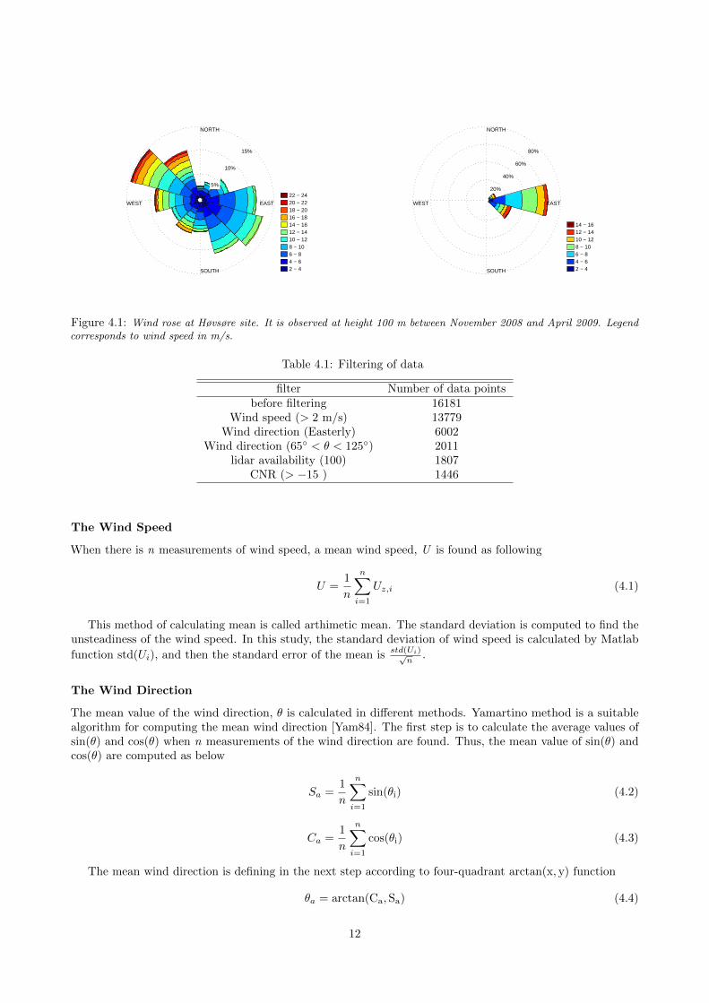
Easterly wind direction has to be analysed between 65 and 125 degrees (figure 4.1), since the wind is distributedmuch more in the interval of 60 and 165 degrees. At Høvsøre, the measurements are influenced by thecharacteristics of the surrounding land. It should take a narrower upwind sector that the average distancewinds have to travel from the land to the mast is reduced. A narrower sector is not chosen because the numberof available measurements are highly reduced [Flo13]. The wind direction is measured with vane, lidar andsonic at different heights. All directions at all heights are assumed to be in this sector.

Lidar Availability

Lidar availability is the percentage of data within an averaging period (10-min) in which the carrier to noiseratio is lower than a threshold value (-28 dB) [Pen09].

Lidar CNR

The carrier to noise ratio is the ratio between the intensity of the received backscatter signal and the intensityof the measured level of noise, and the unit of CNR is in decibels (dB). The value of CNR is considered formore than -15 dB in this study.

The number of data before filtering of all 4 steps that is explained above is 16181. The table 4.1 shows thenumber of data after each step that the measurements are retrieved. For instance, the amount of data has beenreduced from 16181 to 13779 when the wind speed more than 2 m/s is considered. Then, they decrease to 6002when the measurements are retrieved as the Easterly wind. Hence, the number of measurements are reduced to1446 after all the filtering process are carried out and they are in the interval between November 2008 andApril 2009. All of the instruments cover the same amount of data with the same time period.

4.2 Data Averaging

In this section the mean value of wind speed and wind direction will be computed. In this study data are basedon 10-min wind speed and wind direction.

11

5%

10%

15%

WEST EAST

SOUTH

NORTH

2 − 44 − 66 − 88 − 1010 − 1212 − 1414 − 1616 − 1818 − 2020 − 2222 − 24

20%

40%

60%

80%

WEST EAST

SOUTH

NORTH

2 − 44 − 66 − 88 − 1010 − 1212 − 1414 − 16

Figure 4.1: Wind rose at Høvsøre site. It is observed at height 100 m between November 2008 and April 2009. Legendcorresponds to wind speed in m/s.

Table 4.1: Filtering of data

filter Number of data pointsbefore filtering 16181

Wind speed (> 2 m/s) 13779Wind direction (Easterly) 6002

Wind direction (65◦ < θ < 125◦) 2011lidar availability (100) 1807

CNR (> −15 ) 1446

The Wind Speed

When there is n measurements of wind speed, a mean wind speed, U is found as following

U =1

n

n∑i=1

Uz,i (4.1)

This method of calculating mean is called arthimetic mean. The standard deviation is computed to find theunsteadiness of the wind speed. In this study, the standard deviation of wind speed is calculated by Matlab

function std(Ui), and then the standard error of the mean is std(Ui)√n

.

The Wind Direction

The mean value of the wind direction, θ is calculated in different methods. Yamartino method is a suitablealgorithm for computing the mean wind direction [Yam84]. The first step is to calculate the average values ofsin(θ) and cos(θ) when n measurements of the wind direction are found. Thus, the mean value of sin(θ) andcos(θ) are computed as below

Sa =1

n

n∑i=1

sin(θi) (4.2)

Ca =1

n

n∑i=1

cos(θi) (4.3)

The mean wind direction is defining in the next step according to four-quadrant arctan(x, y) function

θa = arctan(Ca,Sa) (4.4)

12

The right hand of Eq. (4.4) is expressed as atan2(Ca,Sa) in MATLAB codes, and in addition the unit of θis in radian.

At last Yamartino defined standard deviation, σθ is computed as

E =√

1− (S2a + C2

a) (4.5)

σθ = arcsin(E)(1 +2√3

)(E3). (4.6)

The standard error of the mean can be calculated as σθ√n

, where n is the number of measurements [Yam84].

In both cases, the uncertainty of measurements of the wind speed and wind direction are indicated using errorbars.

In the following, it will be shown the difference in the calculation of the mean wind direction and thestandard deviation based on the Yamartino method or the arthimetic mean. Three random directions, 10, 25and 85 degrees in the first quadrant are chosen. The results of the mean value in both methods are illustratedin table 4.2. The result of Yamartino method shows that the mean wind direction is 1.1 degree larger thanthe arthimetic mean. The standard deviation result that is found from the Yamartino method is 2.1 degreessmaller than the other one. There is a significant difference between both methods. If the accurate method isnot used, the predictions become less precise.

Table 4.2: The results of mean and standard deviation in two different methods

Methods Mean value Standard deviationThe Yamartino method 40 37.8

The normal method 38.9 39.9

13

5 Results

Linear regression analysis deals with modelling between two variables, y and x. In the present study, it isapplied to the horizontal mean wind speed (mean wind direction) between lidar wind speed (wind direction)and reference wind speed (wind direction) [Coh+03]. The model is

y = kx+ C (5.1)

where y and x are lidar and reference wind speed (wind direction), and k and C define as regression slope andoffset. Furthermore, there is a determination coefficient,R2 to understand how the variables are correlated. Inthis study, the reference wind speed and wind direction are sonic anemometer and wind vane at height 10 m,respectively.

In this study, first, data filtering is carried out between cup and lidar wind speed at heights 60 m and 100m, and different CNR are checked to find the value which has less signal noise and errors. Then, this process ischecked between the vane and lidar wind directions. Figure 5.1 illustrates correlations for different CNR valuesat height 100 m between lidar-cup wind speeds and lidar-vane wind directions. In figure 5.2, when the value ofCNR increases, the number of measurements decreases. Therefore, when figure 5.1 is complemented with figure5.2, CNR value is chosen larger than -15 dB, in order to have sufficient number of measurements and highvalue of R2.

−30 −25 −20 −15 −10 −50.9978

0.9978

0.9979

0.9979

0.998

0.998

0.9981

0.9981

0.9982

0.9982

CNR [dB]

R2

10-min wind speed

−30 −25 −20 −15 −10 −5

0.9927

0.9927

0.9927

0.9927

0.9927

0.9928

0.9928

0.9928

0.9928

0.9928

CNR [dB]

R2

10-min wind direction

Figure 5.1: Correlations for different CNR values between lidar and cup wind speeds at height 100 m (left panel), andbetween lidar and vane wind directions at height 100 m (right).

−30 −25 −20 −15 −10 −50

200

400

600

800

1000

1200

1400

1600

1800

2000

CNR [dB]

Numberofdata

10-min wind speed

−30 −25 −20 −15 −10 −51806

1806.2

1806.4

1806.6

1806.8

1807

1807.2

1807.4

1807.6

1807.8

1808

CNR [dB]

Numberofdata

10-min wind direction

Figure 5.2: The number of data for different CNR values between lidar and cup wind speeds at height 100 m (left panel),and between lidar and vane wind directions at height 100 m (right).

Figure 5.3 shows a scatter plot of 10-min mean wind speed measured by the cup and sonic anemometerscompared to that from the wind lidar at 100 m for the whole period. In this figure, there is good agreementsbetween the wind speed from the lidar and the cup and sonic anemometers. It is seen in figure 5.3 that R2

at both heights 100 m and 60 m are almost 0.99 which shows how well the wind speed distributions in theseinstruments are correlated. The lidar-cup wind speed comparison shows a slope very close to 1 but in the

14

lidar-sonic one is 0.97, i.e. 3 percent higher wind speeds than the sonic. This is because the sonic overestimatesthe wind speed. It is expected that the cup overestimates the wind speed contains a contribution from traverseturbulence fluctuations. It was explained in the previous section that the drawback of sonic anemometer is thatit produces wind speed errors.

0 5 10 150

2

4

6

8

10

12

14

16

18

Cup Wind Speed [m/s]

LidarW

indSpeed[m

/s]

y = 0.99x+ 0.006(100m)

R2 = 0.9981y = 0.99x− 0.045(60m)

R2 = 0.9979

Height 100mHeight 60m

0 5 10 150

2

4

6

8

10

12

14

16

18

Sonic wind speed [m/s]

Lidarwindspeed[m

/s]

y = 0.97x+ 0.04(100m)

R2 = 0.9980y = 0.97x+ 0.009(60m)

R2 = 0.9978


Figure 5.3: Regression for mean wind speeds at heights 60 m (red dots) and 100 m (blue dots) in lidar, cup and sonic.At each height regression slope, offset and regression coefficient are calculated.

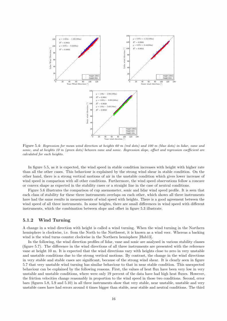
The same process as explained above is used for linear regression analysis of the mean wind directions. Infigure 5.4, R2 indicates that there are good correlations between lidar, vane and sonic which is around 0.99.The lidar-vane wind direction comparison shows a slope very close to 1, whereas the slope in lidar-sonic is equalto 0.97. This difference in slope shows that the sonic overestimates the wind direction. There is a noticeableoffset at height 100 m, for which sonic-lidar is +1.55 degrees, vane-lidar is -1.23 degrees and vane-sonic is -2.66degrees. It means, for example, when sonic at height 100 m shows zero degree, lidar indicates 1.55 degrees.The offset of the wind direction does not necessarily mean that the wind lidar is wrong but that the sonic orvane are not perfectly aligned with the North or at least with the geographical North of the lidar.

5.1 The effect of stability

5.1.1 Vertical Wind Shear

Wind shear is the change in the wind speed with height in the atmosphere. In Eq. (2.2),du

dzrepresents the

wind shear influenced by the atmospheric stability.The wind profile is considered according to its dependency on z/L in Eq. (2.5). The 10-min wind profile

will be classified into different stability classes according to L. The wind characteristics within each stabilityclasses are analysed. Table 5.1 indicates different ranges of stabilities, which are divided in very stable to veryunstable according to the Obukhov length.

Table 5.1: Different stability classes according to Obukhov length [Pen09]

Stability Class Interval of Obukhov length L [m]Very stable (vs) 10 ≤ L ≤ 50

Stable (s) 150 ≤ L ≤ 200Near Stable (ns) 200 ≤ L ≤ 500

Neutral (n) 500 ≤ L,L ≤ −500Near unstable (nu) −500 ≤ L ≤ −200

Unstable (u) −200 ≤ L ≤ −100Very unstable (vu) −100 ≤ L ≤ −50

It is seen in figure 5.5 how the mean value of U/u∗ changes with logarithmic heights in different stabilityclasses when lidar, cup and sonic are used. These measurements have been carried out at Høvsøre site andafter filtering in the period between November 2008 and April 2009.

15

0 20 40 60 80 100 1200

20

40

60

80

100

120

Vane Wind Direction [◦]

LidarW

indDirection[◦]

y = 1.024x− 1.23(100m)

R2 = 0.9931

y = 0.97x− 0.3(60m)

R2 = 0.9893


0 20 40 60 80 100 120 1400

20

40

60

80

100

120

140

Sonic wind direction [◦]

Lidarwinddirection[◦]

y = 0.97x+ 1.55(100m)

R2 = 0.9908

y = 0.97x+ 0.44(60m)

R2 = 0.9934


0 20 40 60 80 100 120 1400

20

40

60

80

100

120

140

Vane wind direction [◦]

Son

icwinddirection

[◦]

y = 1.06x− 2.66(100m)

R2 = 0.9981

y = 1.001x− 0.001(60m)

R2 = 0.9928

y = 1.04x− 5.65(10m)

R2 = 0.9959

Height 100mHeight 60mHeight 10m

Figure 5.4: Regression for mean wind direction at heights 60 m (red dots) and 100 m (blue dots) in lidar, vane andsonic, and at heights 10 m (green dots) between vane and sonic. Regression slope, offset and regression coefficient arecalculated for each heights.

In figure 5.5, as it is expected, the wind speed in stable condition increases with height with higher ratethan all the other cases. This behaviour is explained by the strong wind shear in stable condition. On theother hand, there is a strong vertical motions of air in the unstable condition which gives lower increase ofwind speed in comparison with all other conditions. Furthermore, the wind speed observations follow a concaveor convex shape as expected in the stability cases or a straight line in the case of neutral conditions.

Figure 5.6 illustrates the comparison of cup anemometer, sonic and lidar wind speed profile. It is seen thateach class of stability for these three instruments overlaps on each other, which shows all three instrumentshave had the same results in measurements of wind speed with heights. There is a good agreement between thewind speed of all three instruments. In some heights, there are small differences in wind speed with differentinstruments, which the combination between slope and offset in figure 5.3 illustrate.

5.1.2 Wind Turning

A change in a wind direction with height is called a wind turning. When the wind turning in the Northernhemisphere is clockwise, i.e. from the North to the Northwest, it is known as a wind veer. Whereas a backingwind is the wind turns counter clockwise in the Northern hemisphere [Hab13].

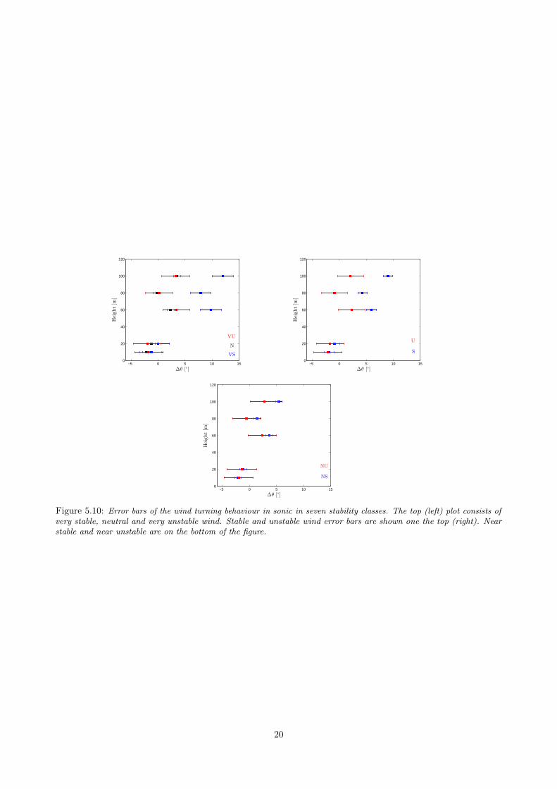
In the following, the wind direction profiles of lidar, vane and sonic are analysed in various stability classes(figure 5.7). The difference in the wind directions of all three instruments are presented with the referencevane at height 10 m. It is expected that the wind directions vary with heights close to zero in very unstableand unstable conditions due to the strong vertical motions. By contrast, the change in the wind directionsin very stable and stable cases are significant, because of the strong wind shear. It is clearly seen in figure5.7 that very unstable wind turning has similar behaviour to that in near stable condition. This unexpectedbehaviour can be explained by the following reasons. First, the values of heat flux have been very low in veryunstable and unstable conditions, where were only 19 percent of the data have had high heat fluxes. However,the friction velocities change reasonably in proportion to the wind speed in those two conditions. Second, errorbars (figures 5.8, 5.9 and 5.10) in all three instruments show that very stable, near unstable, unstable and veryunstable cases have had errors around 4 times bigger than stable, near stable and neutral conditions. The third

16

10 20 30 40 50 6020

40

60

80

100

120

160

200

U/u∗ [-]

Height[m

]

Lidar

VSSNSNNUUVU

10 20 30 40 50 6020

40

60

80

100

120

U/u∗ [-]

Height[m

]

Cup

VSSNSNNUUVU

10 20 30 40 50 60

20

40

60

80

100

U/u∗ [-]

Height[m

]

Sonic

VSSNSNNUUVU

Figure 5.5: Wind profile of lidar (top left), cup (top right) and sonic (on the bottom) in different stability classes.Legend information is given in Table 5.1.

reason is the number of measurements in those four cases have been smaller than 40 which is considered as low.The other reason which may affect the wind turning is baroclinity but is not considered in this study. Floors

explained that baroclinicity has a large effect on the wind veer in the boundary layer because the forcing ischanging with height. He mentioned in his thesis report that the effect of baroclinicity on the wind profilein the boundary layer was recognized a long time ago and studying its influence is often based on large-eddysimulation data [Flo13]. In the case of very unstable and unstable conditions, there are two days (November 29of 2008 and April 15 of 2009) that the change in the wind directions has not been similar as the other data. Itmeans that the wind direction, instead of changing around zero degree, has a higher variation with differentshape. Around two third of the measurements in very unstable condition and about half of data in unstablecase follow this behaviour.

Another unexpected behaviour is related to the shape of the sonic wind direction profile. Each stability classdoes not follow its concave or convex shape or a straight line. This behaviour shows that the sonic anemometersat different heights are probably not mounted exactly to the North, and they are installed with an offset.

Figure 5.8, 5.9 and 5.10 show the error bars of lidar, vane and sonic wind turning, respectively. In all threeinstruments, stable, near stable and neutral conditions have small variability around 0.8, 0.6 and 0.6 degrees.By contrast, near unstable, unstable and very unstable error bars are approximately changed 2.6, 2.5 and2.4 degrees. These variabilities indicate low certain behaviour of near unstable, unstable and very unstableobservations.

17

15 20 25 30 35 40 45 50 55 6010

20

40

60

80

100

130

160

200

U/u∗ [-]

Height[m

]

VSS

NS

N

NU

UVU

+ Lidar

o Cup

Sonic

Figure 5.6: Comparison of lidar, cup and sonic wind profile at different stability classes and heights. Lidar shows withplus sign, sonic with square and cup with circle. Different colors are related to different stability.

0 2 4 6 8 10 12 1420

40

60

80

100

120

140

160

180

200

∆θ [◦]

Height[m

]

Lidar

VSSNSNNUUVU

0 2 4 6 8 10 12 140

10

20

40

60

80

100

∆θ [◦]

Height[m

]

Vane

VSSNSNNUUVU

−5 0 5 10 150

10

20

30

40

50

60

70

80

90

100

110

∆θ [◦]

Height[m

]

Sonic

VSSNSNNUUVU

Figure 5.7: The wind direction changes with heights in various stability classes in lidar (top left), vane (top right)and sonic (on the bottom). ∆θ indicates the difference in wind direction in each instrument from reference vane winddirection at height 10 m.

18

−4 −2 0 2 4 6 8 10 12 14 160

20

40

60

80

100

120

140

160

180

200

∆θ [◦]

Height[m

]

VS

N

VU

−4 −2 0 2 4 6 8 10 12 14 160

20

40

60

80

100

120

140

160

180

200

220

∆θ [◦]

Height[m

]

S

U

−4 −2 0 2 4 6 8 10 12 14 160

20

40

60

80

100

120

140

160

180

200

220

∆θ [◦]

Height[m

]

NS

NU

Figure 5.8: Error bers of the wind turning behaviour in lidar in seven stability classes. The top (left) plot consists ofvery stable, neutral and very unstable wind. Stable and unstable wind error bars are shown on the top (right). Nearstable and near unstable are on the bottom of the figure.

−4 −2 0 2 4 6 8 10 12 14 160

20

40

60

80

100

120

∆θ [◦]

Height[m

]

VS

N

VU

−4 −2 0 2 4 6 8 10 12 14 160

20

40

60

80

100

120

∆θ [◦]

Height[m

]

S

U

−4 −2 0 2 4 6 8 10 12 14 160

20

40

60

80

100

120

∆θ [◦]

Height[m

]

NS

NU

Figure 5.9: Error bars of the wind turning behaviour in vane in seven stability classes. The top (left) plot consists ofvery stable, neutral and very unstable wind. Stable and unstable wind error bar is shown on the top (right). Near stableand near unstable are on the bottom of the figure.

19

−5 0 5 10 150

20

40

60

80

100

120

∆θ [◦]

Height[m

]

VS

N

VU

−5 0 5 10 150

20

40

60

80

100

120

∆θ [◦]

Height[m

]

S

U

−5 0 5 10 150

20

40

60

80

100

120

∆θ [◦]

Height[m

]

NS

NU

Figure 5.10: Error bars of the wind turning behaviour in sonic in seven stability classes. The top (left) plot consists ofvery stable, neutral and very unstable wind. Stable and unstable wind error bars are shown one the top (right). Nearstable and near unstable are on the bottom of the figure.

20

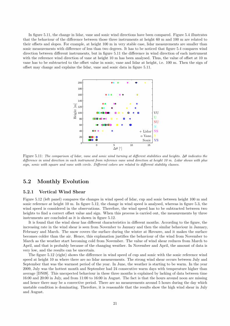
In figure 5.11, the change in lidar, vane and sonic wind directions have been compared. Figure 5.4 illustratesthat the behaviour of the difference between those three instruments at height 60 m and 100 m are related totheir offsets and slopes. For example, at height 100 m in very stable case, lidar measurements are smaller thansonic measurements with difference of less than two degrees. It has to be noticed that figure 5.4 compares winddirection between different instruments, but in figure 5.11 the difference in wind direction of each instrumentwith the reference wind direction of vane at height 10 m has been analysed. Thus, the value of offset at 10 mvane has to be subtracted to the offset value in sonic, vane and lidar at height, i.e. 100 m. Then the sign ofoffset may change and explains the lidar, vane and sonic data in figure 5.11.

0 5 10 150

20

40

60

80

100

120

140

160

180

200

∆θ [◦]

Height[m

]

VS

S

NS

N

NU

U

VU

+ Lidar

o Vane

Sonic

Figure 5.11: The comparison of lidar, vane and sonic wind turning at different stabilities and heights. ∆θ indicates thedifference in wind direction in each instrument from reference vane wind direction at height 10 m. Lidar shows with plussign, sonic with square and vane with circle. Different colors are related to different stability classes.

5.2 Monthly Evolution


Figure 5.12 (left panel) compares the changes in wind speed of lidar, cup and sonic between height 100 m andsonic reference at height 10 m. In figure 5.12, the change in wind speed is analysed, whereas in figure 5.3, thewind speed is considered in the observations. Therefore, the wind speed has to be subtracted between twoheights to find a correct offset value and sign. When this process is carried out, the measurements by threeinstruments are concluded as it is shown in figure 5.12.

It is found that the wind shear has different characteristics in different months. According to the figure, theincreasing rate in the wind shear is seen from November to January and then the similar behaviour in January,February and March. The snow covers the surface during the winter at Høvsøre, and it makes the surfacebecomes colder than the air. Hence, this explanation justifies the behaviour of the wind from November toMarch as the weather start becoming cold from November. The value of wind shear reduces from March toApril, and that is probably because of the changing weather. In November and April, the amount of data isvery low, and the results can be uncertain.

The figure 5.12 (right) shows the difference in wind speed of cup and sonic with the sonic reference windspeed at height 10 m where there are no lidar measurements. The strong wind shear occurs between July andSeptember that was the warmest period of the year. In June, the weather is starting to be warm. In the year2009, July was the hottest month and September had 24 consecutive warm days with temperature higher thanaverage [DN09]. This unexpected behaviour in these three months is explained by lacking of data between time16:00 and 20:00 in July, and from 11:00 to 16:00 in August. The fact is that the hours around noon are missingand hence there may be a convective period. There are no measurements around 5 hours during the day whichunstable condition is dominating. Therefore, it is reasonable that the results show the high wind shear in Julyand August.

21

The error bar in figure 5.12 (left) shows that data reliability on November and April is smaller than theother months, due to high variabilities in November and April. The same explanation is valid for July, Augustand September (Figure 5.12, right).

Nov Dec Jan Feb Mar Apr1

1.5

2

2.5

3

3.5

4

4.5

5

Time [Month]

∆U

[m/s]

Lidar 200mLidar 100mCup 100mSonic 100m

Nov Dec Jan Feb Mar Apr May Jun Jul Aug Sep Oct2

2.5

3

3.5

4

4.5

Time [Month]

∆U

[m/s]

Cup 100mSonic 100m

Figure 5.12: Wind shear in lidar, cup and sonic from December 2008 to April 2009 (left). ∆U indicates the differencein wind speed of each instrument from reference sonic wind speed at height 10 m. The figure (right) is sonic and cupwind shear without considering lidar during 12 months (from November 2008 to October 2009). Error bars of both casesare shown in the figure.

5.2.2 Wind Turning

Figure 5.13(left) compares the wind turning in lidar, vane and sonic which have been measuring the change inwind direction between heights 100 m and the reference vane at 10 m. Besides, the difference in wind directionis indicated in the same plot for lidar at 200 m. As it is clarified in the previous section, figure 5.4 shows theoffset in wind direction for lidar, vane and sonic, while figure 5.13 shows the difference in wind direction. Theoffset value is found according to the difference in wind direction, the offset sign may change. This is becausethe vane, sonic and lidar measurements are located differently at the same height in figure 5.13.


4

6

8

10

12

14

16

18

Time [HH:MM]

∆θ[◦]

Lidar 200mLidar 100mVane 100mSonic 100m

Nov Dec Jan Feb Mar Apr May Jun Jul Aug Sep Oct

2

4

6

8

10

12

14

16

18

Time [Month]

∆θ[◦]

Vane 100mSonic 100m

Figure 5.13: Wind turning behaviour in lidar, vane and sonic from December 2008 to April 2009 (left). ∆θ indicatesthe difference in wind direction in each instrument from reference vane wind direction at height 10 m. The figure (right)is sonic and vane wind turning without considering lidar during 12 months (from November 2008 to October 2009).Error bars of both cases are shown in the figure.

There is a significant reduction in ∆θ from November to December in figure 5.13 (left). It is expected thatthe strong vertical motion occurred in November, because of the wind shear behaviour in figure 5.12. Thisdistinction probably happens, due to the different choice of reference. The other reason is related to errors inNovember and April that are big compare to other months. Furthermore, as explained before, two days in

22

November and April wind behaves differently which has an effect on the wind turning in very unstable andunstable cases and they behave similar to stable winds. Figure 5.14 shows the number of measurements thatexist in every month and based on different stability classes. The fewest amount of data is in November andthen April. In November, there is only three days measurements.

The variation of the wind turning in January, February and March is small. It means that the wind turninghas had a similar behaviour in these three months.


50

100

150

200

250

Time [Months]

Number

ofdata

VSSNSNNUUVU

Figure 5.14: The amount of data that is classified by months and each stability classes. Different colors are related toeach stability conditions.

Figure 5.13 (right) shows the change in the wind direction between November 2008 and October 2009 whenlidar is not considered in the measurements. In this comparison, only vane and sonic are investigated to observehow the wind turning acts in the other months. The wind turning is assumed between the height 100 m ofthe vane and sonic and the reference vane at height 10 m. From June the variation in wind direction goes upand then there is a sharp reduction in October. As it is explained in subsection 5.2.1, in July and August themeasurements do not exist during 5 hours in a day. It shows that data is related much more to those timesthat there is stable condition. Hence, the high change in the wind turning from June to July, and then thesharp reduction in October is related to low amount of data during the day (unstable condition). In conclusion,the wind shear characteristics are in the agreement with the wind turning in the duration of one year.

Error bar in figure 5.13 (right) illustrates the measurements in July, August and September have been moreuncertain due to fewer measurements and high variabilities in these months.

5.3 Daily Evolution


The difference in wind speed during average of 24 hours of the whole 6 months is shown in figure 5.15. Thepurpose of expressing average 24 hours in the whole period or different months is that the time is divided in to24 hours with the interval of one hour. For instance, one of the period is from time 00:00 to 1:00 (00:00 is equalto time 24:00) and then all of the measurements in a month, i.e. December, or the whole duration in this onehour are collected and the mean values of them are calculated. In addition, the changes in the wind speeds areconsidered between height 100 m and reference sonic 10 m, and wind lidar at 200 m is also checked. Night timeis supposed to be from time 18:00 to 6:00, and a day is defined from 6:00 to 18:00.

In figure 5.15, there is a strong wind shear at night compared to the day time. Therefore, the wind isunstable during the day and has stable behaviour at night, in general. The maximum fluctuation of wind shearis around time 21:00, whereas the lowest wind shear happens at noon as expected. The error bars of daily windshear are illustrated in figure 5.15, which are in the same ranges of uncertainty, and the variability of them issmall.

Figure 5.16 illustrates the average of wind shear every one hour in the whole 24 hours in different months.November is not included in the figure because the number of measurements is very low and the plot does notmake sense. The highest change in wind speed(stable condition) has occurred during time 9:00 to 13:00 in

23

0 200 400 600 800 1000 1200 1400 1600 1800 2000 2200 24001

1.5

2

2.5

3

3.5

4

4.5

5

Time [HH:MM]

∆U

[m/s]


Figure 5.15: Average diurnal comparison of lidar, cup and sonic wind shear from November 2008 to April 2009. ∆Uindicates the difference in wind speed of each instrument from reference sonic wind speed at height 10 m. Error bars ofthe diurnal behaviour of three instruments are shown in this figure.

December. Between time 23:00 and 8:00, ∆U has lower value than the other 24 hours, and besides, the strongwind shear during the day in February is obvious. At night, the surface is colder than the air and it is expectedto be stable condition, but in December it is the opposite. This unexpected behaviour is explained by existingsnow in the winter at Høvsøre site, that during the day the surface is colder than the air. In January, the stablecondition is much more common than unstable, especially at night.

Furthermore, the wind speed has not changed significantly in March 2009, except from time 8:00 to 12:00and 18:00 to 22:00 when the wind shear was reduced. It means that unstable condition is distributed in themorning and at night. Figure 5.16 (on the bottom) shows the change in wind speed in April. It is seen thatthere are not any data in some hours of a day, because the measurements do not exist on those times afterfiltering.

5.3.2 Wind Turning

Figure 5.17 indicates average diurnal wind turning. During a period of about 4 hours in the morning, ∆θ hasbeen close to zero that describes unstable condition. In general, the difference in wind direction during the dayhas been less than during the night and it is in agreement with expectations. The diurnal wind shear and thewind turning in the period of six months are proportional to each other, except between time 22:00 and 2:00when they behaved in opposite.

It is seen in figure 5.18 how the wind direction changes during the average 24 hours in five different months.When the change in the wind direction is close to zero, it means there is an unstable wind which usuallyhappened during the day when the surface is warmer than the air and the heat flux is high.

In December after 18:00, the wind turning has a reduction rate, which shows unstable condition occurredduring the night. The wind direction has a fluctuation rate between 6:00 and 18:00, but it increased in general.This unexpected behaviour is justified as explained for the wind shear in the previous subsection. The mostunstable wind behaviour happens in the morning in January. The wind turning has had much more fluctuationduring the day in February, and besides it has been generally in stable condition at night.

In March, as it is expected, the wind direction difference has been generally small during the day, especiallybetween 9:00 and 16.00. This means that there is unstable wind during the day and vice versa at night. As itwas described in the wind shear subsection, there are no measurements in some hours in April, which explainsthat its diurnal behaviour is not precise. Wind lidar at 200 m has almost the same pattern as the otherinstruments in different months, but with higher uncertainty.

24

0 200 400 600 800 1000 1200 1400 1600 1800 2000 2200 24001

2

3

4

5

6

7

Time [HH:MM]

∆U

[m/s]

December


0 200 400 600 800 1000 1200 1400 1600 1800 2000 2200 24001

2

3

4

5

6

7

Time [HH:MM]∆U

[m/s]

January


0 200 400 600 800 1000 1200 1400 1600 1800 2000 2200 24000

1

2

3

4

5

6

7

8

Time [HH:MM]

∆U

[m/s]

February


0 200 400 600 800 1000 1200 1400 1600 1800 2000 2200 24001

2

3

4

5

6

7

Time [HH:MM]

∆U

[m/s]

March


0 200 400 600 800 1000 1200 1400 1600 1800 2000 2200 2400−1

0

1

2

3

4

5

6

7

Time [HH:MM]

∆U

[m/s]

April


Figure 5.16: Lidar, cup and sonic wind shear behaviour on December, January, February, March and April duringaverage 24 hours. ∆U indicates the difference in wind speed of each instrument from reference sonic wind speed at height10 m. Error bars of wind shear behaviour in lidar, cup and sonic are shown in the figure.

25

0 200 400 600 800 1000 1200 1400 1600 1800 2000 2200 2400−2

0

2

4

6

8

10

12

14

16

Time [HH:MM]

∆θ[◦]


Figure 5.17: Average diurnal comparison of lidar, vane and sonic wind turning from November 2008 to April 2009. ∆θindicates the difference in wind direction in each instrument from reference vane wind direction at height 10 m. Errorbars of the diurnal behaviour of three instruments are shown in this figure.

26

0 200 400 600 800 1000 1200 1400 1600 1800 2000 2200 2400−2

0

2

4

6

8

10

12

14

16

18

Time [HH:MM]

∆θ[◦]

December


0 200 400 600 800 1000 1200 1400 1600 1800 2000 2200 2400−10

−5

0

5

10

15

20

25

Time [HH:MM]∆θ[◦]

January


0 200 400 600 800 1000 1200 1400 1600 1800 2000 2200 24000

5

10

15

20

25

30

Time [HH:MM]

∆θ[◦]

February


0 200 400 600 800 1000 1200 1400 1600 1800 2000 2200 2400−5

0

5

10

15

20

25

30

35

Time [HH:MM]

∆θ[◦]

March


0 200 400 600 800 1000 1200 1400 1600 1800 2000 2200 24000

5

10

15

20

25

30

35

40

Time [HH:MM]

∆θ[◦]

April


Figure 5.18: Lidar, vane and sonic wind turning behaviour on December, January, February, March and April duringaverage 24 hours. ∆θ indicates the difference in wind direction in each instrument from reference vane wind direction atheight 10 m. Error bars in mean diurnal wind turning behaviour in lidar, vane and sonic are shown in this figure.

27

5.4 Non-dimensionalization

Non-dimentionalization is often employed to reduce the number of parameters and to better reveal thecharacteristics of a system. In figure 5.11 and 5.6, it is seen in the wind speed and wind direction profile thateach stability conditions has different slopes. In this section, the case is to merge the 7 stability classes with7 slopes, and find one slope. In the following, it will be shown whether it is possible to find the equation tocalculate the wind speed and wind direction at each height, specially, at those heights for which the instrumentsare not mounted.


The wind profile of different stability classes are plotted in subsection 5.1.1. Each of seven stability classes haddifferent wind shear characteristics. Every instrument measures the wind speed and wind direction at variousheights. As the ABL is a mixture of all kinds of stability cases, each of these ones has different boundary layerheights (zi). For example, stable layer is in the lower height more common than neutral or unstable cases. Inthe scaling height, z/zi, different values for zi in each stability classes are checked until all of them collapsed inone line. This process is carried out for U/u∗ versus logarithmic value of z/zi for different instruments, whichare lidar, cup and sonic. Table 5.2 shows the values of boundary layer heights related to each stability class atHøvsøre site.

Table 5.2: Value of zi for different stability classes after non-dimensionalization.

Different stability classes zi [m]Very stable 50

Stable 200Near stable 460

Neutral 750Near unstable 770

Unstable 1100Very unstable 1400

Figure 5.19 collects the non-dimensionalized velocity profiles under different stability conditions and measuredwith all three instruments. As can be seen, the non-dimensionalized velocity profile is shared by various stabilityconditions. All of these three instruments with their collapsed data are compared in a figure 5.20. It is seen allof them are approximately in the same line which is a polynomial degree 2.

The relation between z/zi and U/u∗ is found according to the following

U

u∗= 1.41(ln

z

zi)2 + 11.2(ln

z

zi) + 40.35 (5.2)

U

u∗= 28/k[(ln

z

zi) + 7.95(ln

z

zi)2 + 2.5] (5.3)

where k = 0.4 is von Karman constant, and z is the height above the ground. U and u∗ are the horizontalwind speed and the friction velocity, respectively. Eq. (5.3) is valid at Høvsøre site.

In figure 5.21, blue dots illustrate that lidar, cup and sonic data collapse on to one line. The red line is thefitted line related to these data, and it is expressed in Eq. (5.3).

5.4.2 Wind Turning

The values of zi that are found for the wind speed in seven stability classes in subsection 5.5.1 (Table 5.2) havebeen used for the wind direction profile. The turning of the winds in different stability conditions have notcollapsed in one line, however this non-dimensionalization occurred for wind speed profile.

Figure 5.22 illustrates non-dimensionalization of lidar, vane and sonic wind turning. Very stable measurements

have larger slope than other stability conditions. Then,z

ziis considered between zero and 1 to observe whether

other stability conditions are collapsed or not. It is seen that stable, near stable, neutral and near unstable

28

10 20 30 40 50 600.01

1.01

2.01

3.01

5.01

10

U/u∗ [-]

Z/Zi[-]

Lidar

VSSNSNNUUVU

10 20 30 40 50 600.01

1.01

2.01

3.01

5.01

10

U/u∗ [-]

Z/Zi[-]

Cup

VSSNSNNUsUsVUs

10 20 30 40 50 600.001

1.001

2.0013.001

5.001

10

U/u∗ [-]

Z/Zi[-]

Sonic

VSSNSNNUsUsVUs

Figure 5.19: Collapsing of lidar, cup and sonic wind speed variation in different stability classes.

measurements in lidar are close to collapse but not in very unstable and unstable. As it is explained before,very unstable and unstable wind turnings have not shown reasonable characteristics in wind direction profile.Once again in vane and sonic, the shape of profile has not been as expected. Therefore, these unexpectedbehaviours may be affected non-dimensionalized data in lidar, vane and sonic.

29

10 20 30 40 50 600.001

1.001

2.0013.001

5.001

10

U/u∗ [-]

Z/Zi[-]

VS

S

NS

N

NU

U

VU

+ Lidar

o Cup

Sonic

Figure 5.20: the combonation of the collapsed data of lidar, cup and sonic wind speed variation in different stabilityclasses from November 2008 to April 2009. z/zi is logarithmic

15 20 25 30 35 40 45 50 55 60−5

−4

−3

−2

−1

0

1

2

Z/Zi[-]

U/u∗ [-]

datafitted curve

Figure 5.21: Fitting of non-dimensionalized data in lidar, cup and sonic.

30

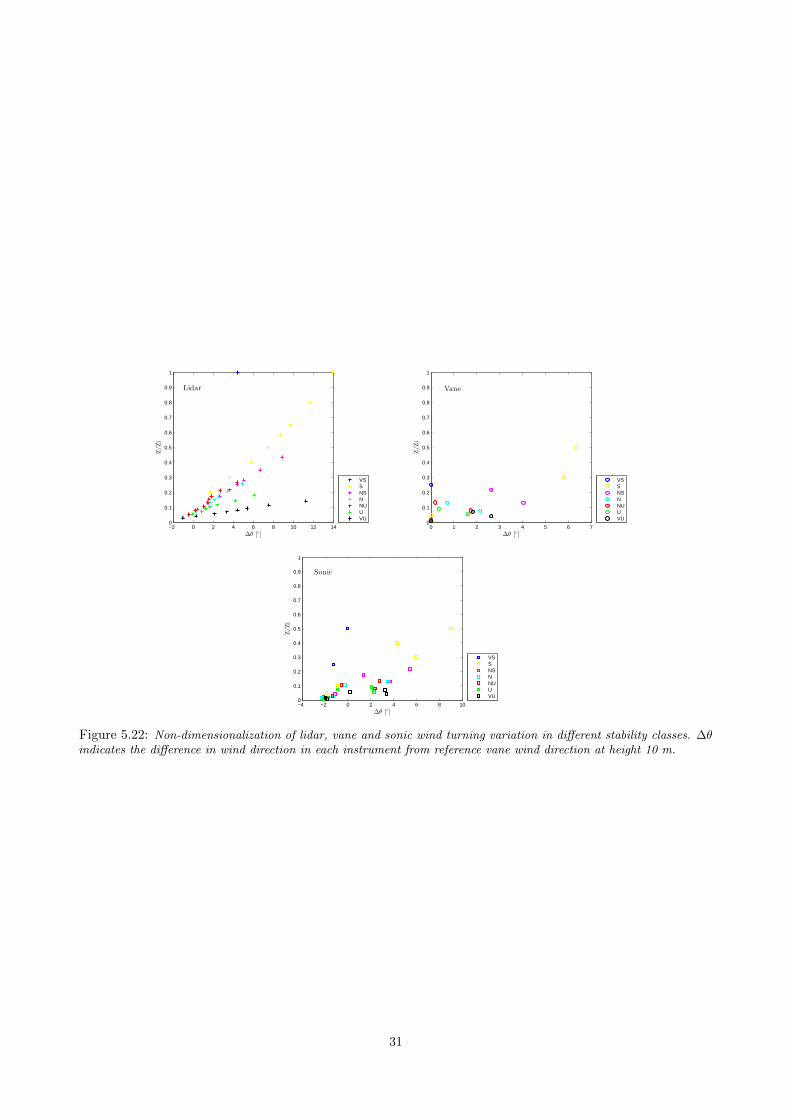
−2 0 2 4 6 8 10 12 140

0.1

0.2

0.3

0.4

0.5

0.6

0.7

0.8

0.9

1

∆θ [◦]

Z/Z

i

Lidar

VSSNSNNUUVU

0 1 2 3 4 5 6 70

0.1

0.2

0.3

0.4

0.5

0.6

0.7

0.8

0.9

1

∆θ [◦]

Z/Zi

Vane

VSSNSNNUUVU

−4 −2 0 2 4 6 8 100

0.1

0.2

0.3

0.4

0.5

0.6

0.7

0.8

0.9

1

∆θ [◦]

Z/Z

i

Sonic

VSSNSNNUUVU

Figure 5.22: Non-dimensionalization of lidar, vane and sonic wind turning variation in different stability classes. ∆θindicates the difference in wind direction in each instrument from reference vane wind direction at height 10 m.

31

6 Discussion

In this section the results of the wind shear and the turning of the wind are analysed. At the end, thecomparison between the wind shear and wind turning are carried out in more detail.

Vertical wind shear and wind turning

The wind speed profiles measured by lidar, cup and sonic at heights below 100 m behave as expected in thesurface layer. The slope of the wind speed profile matches accurately to different stability classes. Furthermore,the wind speed observations by lidar behave as expected between heights 100 m and 200 m. They follow theshape of the stability conditions in agreement with their shape in the surface layer. Therefore, the wind speedobserved by lidar shows the same accuracy as the cup/sonic wind speed measurements.

The wind turning observations by lidar, vane and sonic do not behave as expected in the surface layer.Very unstable wind shows a behaviour similar to near stable condition in all three instruments. In lidar, thewind direction profile follows the shape in agreement with different stability cases, except in very stable andvery unstable conditions. As expected in very stable condition, the change of ∆θ with height approaches toan asymptote at heights above 100 m. An unexpected behaviour is that ∆θ in very unstable and unstableconditions change highly, instead of changing around zero degree. Three reasons could explain these unexpectedresults. First, the heat fluxes are very low in very unstable and unstable conditions. Only a small fraction ofdata shows the convective characteristics. Another explanation could be that the number of measurementsare very low in very unstable and unstable cases. It might have an effect on the uncertainty of measurements.Finally, one day in November and April the change in wind direction in very unstable and unstable conditionshas been similar to near stable case. It means that as the heights increase, the slope of the wind turningbehaviours reduce instead of increase.

In vane and sonic, the shape (concave, convex or straight line) of the wind direction profile does not matchto seven stability classes in the surface layer. The reason might be that the vane and sonic at all heights arenot exactly mounted to the North, and the offset at various heights is different.

The comparison between the Vertical wind shear and wind turning

The wind shear and the wind turning from November 2008 to October 2009 is analysed between cup, vane andsonic without considering lidar. The comparisons between the measurements of cup-sonic and vane-sonic showthat the wind shear and the wind turning from March to April had an increase rate. Since the measurementsexist in all times of 24 hours during both months, they are much more reliable than the measurements in figure5.12 and 5.13 (with lidar observations). Hence, it is predicted that in figure 5.12 and 5.13 (left panel) the windshear and the wind turning should be in an increasing rate from March to April.

The average diurnal wind shear from November to April has been in agreement with the wind turning,however, they have not behaved in the same way in some hours of the whole 24 hours, i.e. from 10:00 to 12:00,and 2:00 to 4:00. This behaviour can be seen in the mean diurnal wind shear and wind turning of each month.The explanation for this result is that the wind turning in very unstable and unstable cases has a behavioursimilar to near stable. Hence, those times which show high ∆θ, they can be stable or unstable wind. The windturning and wind shear might be in agreement but because of very unstable and unstable behaviours, it seemsthey are in contradiction.

Monthly evolution of the wind shear and wind turning shows that the wind shear and the wind turning arein agreement from December to March, but in November and April they behave oppositely. The reason mightbe related to lack of measurements at some times of 24 hours. In April, there are not any data after filteringbetween time 11:00 and 15:00, and from 3:00 to 4:00. It seems that the results have to show high wind shearand wind turning. In November, there is low amount of data, which is distributed during night, and that is thereason ∆θ in November is higher than the other months.

The present study has not investigated the physical effect on wind to figure out exactly the reason ofunexpected behaviour of the wind turning profile. Thus, it is recommended to further study this field and finda further precise justification. Furthermore, the contradiction between wind turning and wind shear in someperiods of time makes the need of more research in the turning of the wind in the future.

32

7 Conclusion

The wind speed and wind direction profile in the ABL have been measured by combining cup, sonic and vaneat meteorological mast with lidar observations overland at Høvsøre, Denmark. This study is carried out byaveraging the 10-min wind speed and wind direction measurements in wide range of atmospheric stabilityconditions from November 2008 to April 2009.

The easterly wind speed measurements within a flat and homogeneous sector show that the variousinstruments have been in a good agreement in different stability classes. By contrast, the changes in the winddirection measurements behave unexpected in very unstable conditions in all three instruments.

The mean wind shear during the average 24 hours from November 2008 to April 2009 shows high wind shearduring night and few hours early in the morning. Therefore, the average diurnal behaviour of wind shear in thewhole period has been in agreement with the expectation. The wind turning shows the same result duringthe whole period. The average daily wind shear are compared to the mean diurnal wind turning in the wholeperiod of measurements. It shows the daily wind shear to be in agreement to the diurnal wind turning.

The significant difference of the mean diurnal wind shear of each month is related to the period of 8:00 to14:00, and 18:00 to 23:00. Between 8:00 and 14:00, the wind shear behaves strongly in December and February,whereas in March it has opposite behaviour. During time 18:00 and 23:00 in December, the change in the windspeed is high, but it behaves vice versa in February and March. The rest of 24 hours in December, Februaryand March, the behaviour of wind shear has been approximately constant. The average daily wind turning ofeach month indicates that the wind turning fluctuations have been high. In January and February, ∆θ has highvalue around noon, whereas in March it shows opposite behaviour. In December, ∆θ varies during differenttimes and it shows stable behaviour after 12:00.

The mean wind shear of six months has behaved as in the same way as the mean wind turning, except inNovember and April. There is lack of data in some hours of the day in these two months. Thus, the wind shearis in agreement with the wind turning during the six months. The comparison between sonic and cup windshear and wind turning are accomplished when the lidar observations are not considered. It shows the monthlywind shear characteristics are in the agreement with yearly wind turning. In conclusion, all of the comparisonsshow that the wind shear is in agreement with the turning of the wind.

The findings of this master study help the understanding of wind turning behaviour in the atmosphere.With the growth of wind energy industry and the increasing size of the wind turbines, there is a need for anaccurate and detailed description of the wind turning in the first 200 m above the ground.

33

References

[Age12] J. M. Agency. Measurement of Surface Wind. 2012. url: http://www.jma.go.jp/jma/jma-eng/jma-center/ric/material/1_Lecture_Notes/CP4-Wind.pdf.

[Amo06] J. Amouroux, ed. Green Energy and Technology. Bentham Science Publishers, July 2006. isbn:9781608052851. doi: 10.2174/97816080528511060101. url: http://www.benthamdirect.org/pages/content.php?9781608052851.

[Ant00] D. J. F. Anthoni. Oceanography - currents and circulation (2) (Dec. 2000).[Ass+09] E. W. E. Association et al. Wind Energy-The facts. Routledge, 2009. isbn: 978184407710.[Ass00] D. W. I. Association. Guided Tour on Wind Energy (Sept. 2000). url: http://ele.aut.ac.ir/

~wind/en/tour/.[BMN13] J. Berg, J. Mann, and M. Nielsen. Notes for DTU course 46100 : Introduction to micro meteorology

for wind energy Department of Wind Energy Report 2013. Vol. 0009. February. DTU Wind Energy,2013, p. 104. isbn: 9788792898.

[Car13a] J.-p. Cariou. Pulsed lidars. 2 (2013), 65–81. url: http://rasei.colorado.edu/wind-research-internal1/Jean_Pierre_Cariou.pdf.

[Car13b] J.-P. Carriou. Pulsed coherent lidars for wind remote sensing. June (2013), 1–23.[Coh+03] J. Cohen et al. Applied multiple regression/correlation analysis for the behavioral sciences. Lawrence

Erlbaum Associates, 2003, p. 703. isbn: 0805822232.[DN09] J. Diebel and J. Norda. Historical Weather For 2009 in Tune near Roskilde, Denmark. 2009. url:

http://weatherspark.com/history/28829/2009/Tune-near-Roskilde-Region-Zealand-

Denmark.[Dub04] U. C. Dublin. The Ekman Spiral. Dec. 2004. url: http://maths.ucd.ie/met/msc/fezzik/Phys-

Met/Ch05-4-Slides.pdf.[Etl02] “Theoretische Meteorologie.pdf”. Ed. by P. D. D. Etling. second. Springer-Verlag Berlin Heidelbeerg,

2002, p. 332. isbn: 978-3-540-75979-9.[Flo13] R. Floors. “Boundary-layer wind profile, measurements and theory Risø-PhD-Report”. PhD thesis.

2013.[Hab13] J. Haby. Veering and backing wind defined. 2013. url: http://www.theweatherprediction.com/

habyhints/48/.[Hun99] R. S. Hunter. Wind speed measurement and use of cup anemometry. 1999.[LC12] J. Lundquist and A. Clifton. How turbulence can impact power performance. Sept. 2012. url: https:

//www.wind-watch.org/documents/how-turbulence-can-impact-power-performance/.[Pen09] A. Pena. “Sensing the wind profile Risø-PhD-Report”. PhD thesis. 2009. isbn: 9788755037090.

url: http://www.risoe.dk/rispubl/reports/ris-phd-45.pdf.[Phi79] M. P. M. Philip B Russell Thomas J Swissler. lidar aerosol measurements (1979).[Rar+09] E. Rareshide et al. Effects of complex wind regimes on turbine performance Proc. American Wind

Energy Association WINDPOWER Conference (Chicago, IL) (2009).[Sat+12] A. Sathe et al. Influence of atmospheric stability on wind turbine loads. Wind Energy (July 2012),

n/a–n/a. issn: 10954244. doi: 10.1002/we.1528. url: http://doi.wiley.com/10.1002/we.1528.[SM09] G. Svensson and A. a. M. Holtslag. Analysis of Model Results for the Turning of the Wind

and Related Momentum Fluxes in the Stable Boundary Layer. Boundary-Layer Meteorology132.2 (June 2009), 261–277. issn: 0006-8314. doi: 10.1007/s10546-009-9395-1. url: http://link.springer.com/10.1007/s10546-009-9395-1.

[Stu88] R. B. Stull. An Introduction to Boundary Layer Meteorology. February. Kluwer Academic, 1988,p. 666. isbn: 9027727686.

[Sys13] T. A. L. M. System. Vertical Motion and Atmospheric Stability. 2013.[Wag+09] R. Wagner et al. The influence of the wind speed profile on wind turbine performance measurements.

Wind Energy 12.4 (2009), 348–362.[WL12] S. Wharton and J. K. Lundquist. Atmospheric stability affects wind turbine power collection.

Environmental Research Letters 7.1 (Mar. 2012), 014005. issn: 1748-9326. doi: 10.1088/1748-9326/7/1/014005. url: http://stacks.iop.org/1748-9326/7/i=1/a=014005?key=crossref.df26a50fc7064a0a7c4f98db89353d29.

[Yam84] R. J. Yamartino. A Comparison of Several ”Single-Pass” Estimators of the Standard Deviation ofWind Direction. Climate and Applied Meteorology 23 (9): 1362–1366 (1984).

34

http://www.jma.go.jp/jma/jma-eng/jma-center/ric/material/1_Lecture_Notes/CP4-Wind.pdf

http://www.jma.go.jp/jma/jma-eng/jma-center/ric/material/1_Lecture_Notes/CP4-Wind.pdf

http://dx.doi.org/10.2174/97816080528511060101

http://www.benthamdirect.org/pages/content.php?9781608052851

http://www.benthamdirect.org/pages/content.php?9781608052851

http://ele.aut.ac.ir/~wind/en/tour/

http://ele.aut.ac.ir/~wind/en/tour/

http://rasei.colorado.edu/wind-research-internal1/Jean_Pierre_Cariou.pdf

http://rasei.colorado.edu/wind-research-internal1/Jean_Pierre_Cariou.pdf

http://weatherspark.com/history/28829/2009/Tune-near-Roskilde-Region-Zealand-Denmark

http://weatherspark.com/history/28829/2009/Tune-near-Roskilde-Region-Zealand-Denmark

http://maths.ucd.ie/met/msc/fezzik/Phys-Met/Ch05-4-Slides.pdf

http://maths.ucd.ie/met/msc/fezzik/Phys-Met/Ch05-4-Slides.pdf

http://www.theweatherprediction.com/habyhints/48/

http://www.theweatherprediction.com/habyhints/48/

https://www.wind-watch.org/documents/how-turbulence-can-impact-power-performance/

https://www.wind-watch.org/documents/how-turbulence-can-impact-power-performance/

http://www.risoe.dk/rispubl/reports/ris-phd-45.pdf

http://dx.doi.org/10.1002/we.1528

http://doi.wiley.com/10.1002/we.1528

http://dx.doi.org/10.1007/s10546-009-9395-1

http://link.springer.com/10.1007/s10546-009-9395-1

http://link.springer.com/10.1007/s10546-009-9395-1

http://dx.doi.org/10.1088/1748-9326/7/1/014005

http://dx.doi.org/10.1088/1748-9326/7/1/014005

http://stacks.iop.org/1748-9326/7/i=1/a=014005?key=crossref.df26a50fc7064a0a7c4f98db89353d29

http://stacks.iop.org/1748-9326/7/i=1/a=014005?key=crossref.df26a50fc7064a0a7c4f98db89353d29

Wind Turning in The Atmospheric Boundary...

Documents

Transcript of Wind Turning in The Atmospheric Boundary...